Neural-network-based parameter estimation for quantum detection

Machine learning (ML) techniques are nowadays routinely employed in many areas of scientific research, as well as for industrial applications [1]. The success of ML tools lies in their versatility to tackle multiple and complex problems and in their universal behavior, i.e. their capability to efficiently reproduce any functional dependence between inputs and outputs [1]. ML techniques have found a fertile ground in physical sciences [2]. In these disciplines, ML techniques are opening new avenues to address complex problems, either for classification tasks, parameter regression, or optimisation purposes, as well as to retrieve fundamental physical concepts [3, 4, 5]. Quantum physical problems are also included in the range of action of ML, as exemplified by the fast-growing number of successful applications of ML techniques in this realm [6, 7]. Among them, we can list the ability of ML to learn quantum measurements [8, 9, 10], as well as to design quantum gates, unitary transformations and protocols for quantum state preparation [11, 12, 13, 14]. Moreover, ML can be also used for state and entanglement classification [15, 16, 17], to generate quantum communication protocols [18], identification of Hamiltonians [19] and to retrieve and model open quantum system dynamics [20, 21, 22, 23]. See [6] and references therein for a comprehensive review on the distinct applications of ML to quantum physics.

Among the different sub-fields in quantum technologies, quantum sensing [24] and quantum metrology [25] have experienced a significant progress, placing them at the forefront of this new generation of technologies harnessing quantum effects. This is primarily a consequence of the progress made during the last decades that has enabled the isolation, control, manipulation, and readout of individual quantum registers [26]. In quantum sensing protocols, the information is encoded in the states (phase and/or populations) of a quantum register which offers unprecedented spatial resolution as this is, typically, of atomic size. As examples of the latter, on the one hand, it is worth mentioning nitrogen-vacancy centers in diamond [27, 28] that possess exceptional coherence properties even at room temperature, and thus they are well suited to quantum detection of biological samples [29, 30, 31]. On the other hand, ion-trap technology has been proved also useful in the realm of quantum sensing and quantum metrology [32, 33, 34]. In addition, different kinds of dynamical decoupling pulse sequences [35, 36] have led to extended coherence times in quantum systems to enhance the precision of determining unknown parameters with the limit provided by the Quantum Fisher Information [37, 38].

So far, different protocols for quantum sensing have been demonstrated in scenarios where the basic coupling mechanism of the sensor and the target can be clearly described whilst, in addition, key target parameters are easily encoded in the harmonic response of the quantum register [39, 40]. Nevertheless, quantum sensors significantly deviate from their ideal response as soon as they fail to meet the demanding approximations required by their working regime (in Sec. 3 we exemplify the latter for the specific scenario of an ¹⁷¹Yb⁺ quantum sensor [34, 41, 42, 43, 44]) or due to uncontrollable interactions with environmental agents. Under these general conditions, the quantum sensor leads to a complex response that challenges the identification of target parameters. In this regard, ML techniques may offer an unrivalled tool to extend the performance of quantum sensors to these complex scenarios, while requiring minimal knowledge of their microscopic description. Therefore, the application of ML to quantum sensing and quantum metrology is receiving an increasing attention focusing, e.g., on the optimization of adaptive estimation protocols [45, 46, 47, 48, 49, 50, 51], and on the calibration of quantum sensors [52].

In this article, we propose a scheme for parameter estimations using a neural network (NN) that takes as input the quantum measurement data obtained by interrogating a quantum sensor. This scheme allows for an efficient and accurate parameter estimation, only requiring minimal knowledge of the underlying physical model. We illustrate our NN-based parameter estimation strategy for quantum magnetometry employing an atomic-size ¹⁷¹Yb⁺ system [34, 41, 42, 43, 44] aiming to detect both frequency and amplitude of an incident electromagnetic field, in a parameter regime where the quantum register presents a complex response, i.e., not harmonic. Note this represents a departure to the regime in which current experiments with ¹⁷¹Yb⁺ are posed [34, 41, 42]. Thus, with the assistance of our method, the scope of quantum detection experiments gets significantly enhanced. In addition, since our NN is only exposed to the training/validation/test dataset obtained from experiments, the establishment of the NN and its ability of parameter estimation do not depend on the physical model of the system. Here, we numerically simulate an experimental data acquisition in realistic physical conditions, including shot noise. The average NN prediction accuracy of the relevant parameters is above $97\%$ when inputting data outside the training set.

The article is organized as follows: In Sec. 2 we introduce the basic tools for ML and NN that will be employed for parameter estimation. In Sec. 3 we briefly introduce the main ingredients for magnetometry using an atomic-size quantum sensor device consisting of a ${}^{171}{\rm Yb}^{+}$ ion [41, 34, 42, 43], while the results for NN parameter estimation are presented in Sec. 4. In Sec. 5, we show the prediction precision limit given by Quantum Fisher Information and compare the estimation from the Bayesian estimator and our NN. Finally, Sec. 6 summarizes the main conclusions of the article.

A feed-forward NN can be used to approximate the function that maps inputs to outputs based on the datasets of input-output examples [1]. During the training process, the parameters of the feed-forward network, i.e. the weights of the connections within layers and the biases of the neurons are optimized iteratively so that the outputs of the network approach the targets within some acceptable errors (cf. Fig. 1 for a schematic representation of the NN). Once the network is properly trained, it enables to estimate the outputs corresponding to the inputs that do not belong to the training set. It is important to note that the NN allows for the training based solely on experimental results, thus only minimal knowledge of the underlying physical model is required.

We construct a NN such that it takes as inputs the data acquired by measuring the quantum register at a number $N_{p}$ of time instants, i.e. the measured data $\textbf{X}=\{x_{1},x_{2},\ldots,x_{N_{p}}\}$, and as outputs we demand a number $n_{a}$ of target parameters to be estimated, denoted by $\textbf{Y}=\{y_{1},y_{2},\ldots,y_{n_{a}}\}$. In the training stage, the data X is fed into the NN with its corresponding known output parameters $\textbf{A}=\{a_{1},a_{2},\ldots,a_{n_{a}}\}$, so that the weights and neural connections within the hidden layers are optimized to achieve $F({\textbf{X}})=\textbf{Y}\approx\textbf{A}$ where $F({\textbf{X}})$ denotes the action of the NN on the input X (cf. Fig. 1)

We define the mean square error $C$ as our cost function

for the training set, where the superscript $j$ accounts for corresponding number among the $N$ examples. The value of $C$ for the validation/test set can be obtained similarly by using the outputs $y_{i}^{j}$ from the corresponding set (i.e. validation and test). We use the gradient descent algorithm to train our NN, where Levenberg-Marquardt backpropagation is applied as it is usually the fastest one. Since the weights and biases are randomly initialised, we train the network several times to obtain statistical-significance values. By applying backward propagation steps and finding partial derivatives of the weights w and the bias b, i.e., $\partial C/\partial\textbf{w}$ and ${\partial C}/{\partial\textbf{b}}$, these trainable parameters of the NN are adjusted to minimize $C$, expressed as

where $\eta$ stands for the learning rate.

In this manner, we achieve the parameter estimation scheme. That is, by introducing the measured data from the quantum register, X, to the NN we approximately obtain the unknown target features, i.e. $F({\textbf{X}})={\textbf{Y}}\approx{\textbf{A}}$, in situations where the sensor presents a non-harmonic response. In the following we illustrate the good performance of our strategy using a ¹⁷¹Yb⁺ ion as a magnetometer [41, 34, 42, 43].

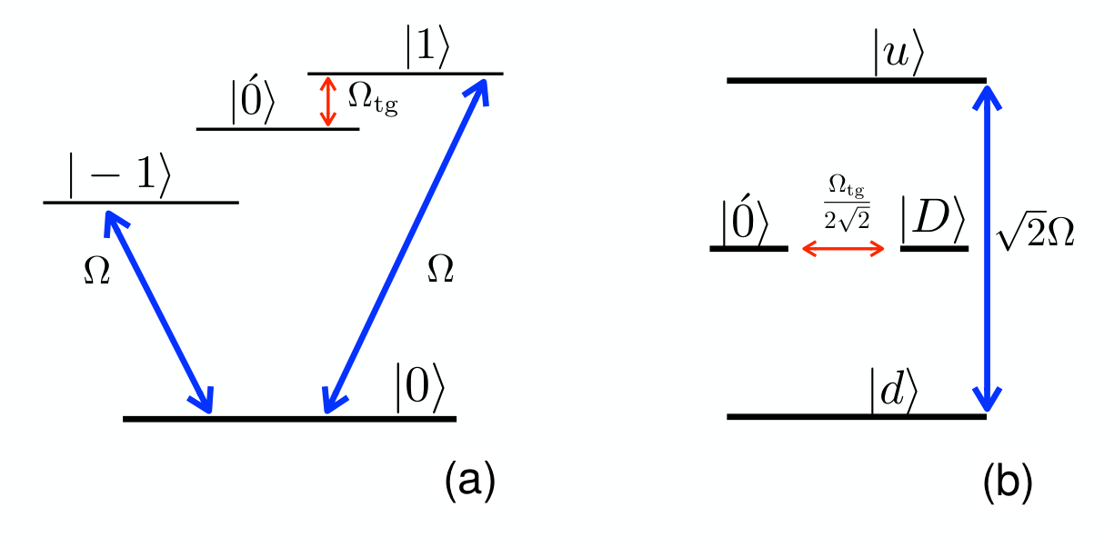
Let us consider an ¹⁷¹Yb⁺ quantum sensor device aimed to detect electromagnetic fields, according to the scheme put forward in [41, 34, 42]. The sensor is encoded in the ${}^{2}S_{\frac{1}{2}}$ manifold of the ¹⁷¹Yb⁺ consisting of four hyperfine levels $|0\rangle$, $|\acute{0}\rangle$, $|1\rangle$ and $|-1\rangle$, where the degeneracy of the states $|\acute{0}\rangle$, $|1\rangle$ and $|-1\rangle$ is lifted by applying a static magnetic field $B_{z}$. In order to cancel the magnetic field fluctuations and achieve long coherence times, we apply two microwave drivings resonant with the $|0\rangle\leftrightarrow|1\rangle$ and $|0\rangle\leftrightarrow|-1\rangle$ hyperfine transitions with amplitudes $\Omega_{1,2}$ respectively, cf. Fig. 2.

A target electromagnetic field of frequency $\omega_{\rm{tg}}$ and amplitude $\Omega_{\rm tg}$, i.e., of the form $\Omega_{\rm{tg}}\cos(\omega_{\rm{tg}}t)$, can be detected by using the $|\acute{0}\rangle\leftrightarrow|1\rangle$ or $|\acute{0}\rangle\leftrightarrow|-1\rangle$ transition. Following the scheme proposed in [34], the target field can be probed assuming that it drives one of the above two transitions, e.g., the $|\acute{0}\rangle\leftrightarrow|1\rangle$ transition with $\omega_{\rm{tg}}=\omega_{1}-\omega_{\acute{0}}+\xi$, where $\xi$ is a small detuning with respect to the resonant condition. In the rotating frame of $\Omega/\sqrt{2}(|u\rangle\langle u|-|d\rangle\langle d|)$ (assuming $\Omega\equiv\Omega_{1,2}$) one finally finds the relevant contributions for the quantum sensor dynamics which is in turn protected against magnetic field fluctuations. More specifically, in the dressed state basis $\left\{|u\rangle,|d\rangle,|D\rangle,|\acute{0}\rangle\right\}$ (cf. Fig. 2) where $|u\rangle=(|B\rangle+|0\rangle)/\sqrt{2}$, $|d\rangle=(|B\rangle-|0\rangle)/\sqrt{2}$, $|D\rangle=(|-1\rangle-|1\rangle)/\sqrt{2}$, $|\acute{0}\rangle=|\acute{0}\rangle$, with $|B\rangle=(|-1\rangle+|1\rangle)/\sqrt{2}$, we measure the response of the sensor $P_{D}(t)$. This is, the survival probability of the state $|D\rangle$ when the target electromagnetic field is acting on the sensor.

As we explain in A, by further assuming that $\xi=0$ and upon a rotating wave approximation ($\Omega_{\rm tg}\ll\Omega\ll\omega_{\rm tg}$) one can find a harmonic/ideal response $P_{D}(t)=\cos^{2}(\pi t/t_{\rm{R}})$, with $t_{\rm{R}}=2\pi\sqrt{2}/\Omega_{\rm{tg}}$. At this point, it is worth mentioning that the conditions $\xi=0$ and $\Omega_{\rm tg}\ll\Omega\ll\omega_{\rm tg}$ determine the working regime of the ¹⁷¹Yb⁺ quantum sensor leading to its ideal harmonic response. In this situation, the populations of the states $|D\rangle$ and $|\acute{0}\rangle$ oscillate at a rate given by $\Omega_{\rm{tg}}/(2\sqrt{2})$, see A. Remarkably, for a possibly detuned electromagnetic field, $\xi\neq 0$, with a large amplitude $\Omega_{\rm tg}$ and/or small frequency $\omega_{\rm tg}$, the sensor abandons its working regime. As a consequence, the sensor response $P_{D}(t)$ no longer follows the ideal harmonic behavior, which challenges the identification of the relevant parameters $\Omega_{\rm tg}$ and $\xi$.

Indeed, a detailed description of the interaction between the internal levels of ¹⁷¹Yb⁺ and the target electromagnetic signal (see  A) reveals a complex sensor response $P_{D}(t)$, that needs to be computed by numerically solving the time-dependent Schrödinger equation. In Fig. 3 we provide three different and illustrative cases for $P_{D}(t)$. As it can be seen in Fig. 3, as soon as $\Omega_{\rm tg}$ becomes comparable to $\Omega$ and/or $\xi\neq 0$, the response $P_{D}(t)$ looses its harmonic behaviour. In the following, we show how an appropriately trained NN is able to extract $\Omega_{\rm tg}$ and $\xi$ even in these challenging situations.

Quantum fisher Information (QFI), constraining the achievable precision in statistical estimation of the parameter $\theta$, for a pure state $|\psi\rangle$ is defined as

where in our scenario $\theta=\Omega_{\rm{tg}}$ or $\xi$. Taking the variance for the parameter estimator encoded in a state at the final time instant $t_{0}$ at which we measure $P_{D}$, we find that the precision is upper bound, or similarly, the variance is lower bound as

where $N_{T}=N_{p}\times N_{m}$ with $N_{p}=101$ the time points at which the state is interrogated, and $N_{m}=100$ measurements of shots per time instant. For instance, in the case of a harmonic response $\Omega_{\rm{tg}}=2\pi\times 1$ kHz and $\xi=0$, we can express the state of the system analytically as

From Eq. (3), we can directly compute $I_{\Omega_{\rm{tg}}}=t^{2}/2$. Consequently, the variance for the estimator of $\Omega_{\rm{tg}}$ should be equal or larger than $\Delta\Omega_{\rm{tg}}^{\rm{QFI}}\approx 2\pi\times 1.5\cdot 10^{-3}$ kHz. For the case of non-harmonic responses, we take the instance $\Omega_{\rm{tg}}=2\pi\times 9.31$ kHz and $\xi=2\pi\times 0.15$ kHz and numerically derive $\Delta\Omega_{\rm{tg}}^{\rm{QFI}}\approx 2\pi\times 3\cdot 10^{-3}$ kHz and $\Delta\xi^{\rm{QFI}}\approx 2\pi\times 7\cdot 10^{-4}$ kHz. Now, we generate $100$ examples in the presence of shot noise from the same targets (i.e. $\Omega_{\rm{tg}}=2\pi\times 9.31$ kHz and $\xi=2\pi\times 0.15$ kHz) and obtain the outputs of the NN trained from the dataset with the range $\Omega_{\rm{tg}}/(2\pi)\in[8.2,25]$ kHz and $\xi/(2\pi)\in[-0.3,0.3]$ kHz. Consequently, we derive the average value $\overline{y}_{1}=2\pi\times 9.3055$ kHz and $\overline{y}_{2}=2\pi\times 0.1523$ kHz with the standard deviation $\sigma_{y_{1}}=2\pi\times 0.0339$ kHz and $\sigma_{y_{2}}=2\pi\times 0.0027$ kHz, which indicates that the precision is below the limit imposed by the QFI.

It is interesting to note that the obtained precision should always be lower than this upper bound for any kind of estimator. Here, we compare the prediction of a NN and a Bayesian estimator which is known to be optimal for large datasets. In particular, we compute the posterior distribution following the well-known Bayes theorem, $p(\theta|{\textbf{X}})\propto p({\textbf{X}}|\theta)p(\theta)$ where $p(\theta)$, $p({\textbf{X}}|\theta)$ and $p(\theta|{\textbf{X}})$ denote the prior, likelihood and posterior distributions. Note that X represents the data obtained by interrogating the quantum sensor at different time instances used to feed the NN. In this case we consider an uninformative prior ($p(\theta)\propto 1$) for the two parameters, while the likelihood is assumed to obey a Gaussian distribution since $N_{m}\gg 1$, that is, $p({\textbf{X}}|\theta)=\Pi_{j=1}^{N_{p}}\frac{1}{\sqrt{2\pi}\sigma_{j}}e^{-(x_{j}-\tilde{x}_{j})^{2}/(2\sigma_{j}^{2})}$ where $\tilde{x}_{j}$ refers to the expectation value of the measured observable, $P_{D}$ at time $t_{j}$ under the parameters $\theta$ and computed following the Hamiltonian in Eq. (8) (see A). As standard deviation we take $\sigma_{j}=1/\sqrt{N_{m}}$. From $p(\theta|{\textbf{X}})$ one can obtain the estimator for $\theta_{j}$ and its variance as $\Delta^{2}\theta_{j}=\int d\theta(\theta_{j}-\overline{\theta}_{j})^{2}p(\theta|{\textbf{X}})$ and $\overline{\theta_{j}}=\int d\theta\theta_{j}p(\theta|{\textbf{X}})$, where integral is performed over the unknown parameters $\theta$. In the example considered above, $\Omega_{\rm tg}=2\pi\times 9.31$ kHz and $\xi=2\pi\times 0.15$ kHz, a Bayesian analysis leads to $\overline{\Omega}_{\rm tg}=2\pi\times 9.31(2)$ kHz and $\overline{\xi}=2\pi\times 0.153(7)$ kHz with $\overline{\Delta\Omega_{\rm tg}}\approx 2\pi\times 2\cdot 10^{-2}$ kHz and $\overline{\Delta\xi}\approx 2\pi\times 7\cdot 10^{-3}$ kHz, which reveals a comparable precision as that obtained with NN. Similar values for the variances are obtained for different datasets and parameters. We remark that, a Bayesian analysis and a NN provide similar precision for the estimators. However, a Bayesian estimator requires a precise microscopic model to compute the evolution for each possible combination of the unknown parameters $\theta$. In this regard, a NN needs less knowledge of the system due to the fact that the training/validation/test datasets only originate from the experimental measurement and the input-output relation is learned, while at the same time allowing for good estimators. Thus, a well-trained NN can accurately provide estimators for the unknown parameters in a wide range set by the training dataset with a minimal knowledge of the underlying physical model.

We have proposed a scheme for quantum parameter estimation using neural networks (NNs) which can effectively reproduce the functional dependence between the input measured data from the quantum register and the target parameters to be estimated. We have illustrated our scheme for magnetometry using an atomic-size sensor encoded in the internal levels of a ¹⁷¹Yb⁺ ion and in a parameter regime where the sensor presents a complex response, far from an ideal harmonic behaviour. The NN allows for an accurate estimation of the amplitude and detuning of the target electromagnetic field for cases which do not belong to the training dataset. Since ML techniques require minimal knowledge of the underlying physical model and are able to tackle complex input-output relations, these tools are best placed to enhance the performance of quantum sensors. We expect that our results will motivate further research and applications of NN in quantum sensing and quantum metrology.

We acknowledge financial support from Spanish Government via PGC2018-095113-B-I00 (MCIU/AEI/FEDER, UE), Basque Government via IT986-16, as well as from QMiCS (820505) and OpenSuperQ (820363) of the EU Flagship on Quantum Technologies, and the EU FET Open Grant Quromorphic (828826). R. P. acknowledges the support by the SFI-DfE Investigator Programme (grant 15/IA/2864). J. C. acknowledges the Ramón y Cajal program (RYC2018-025197-I) and the EUR2020-112117 project of the Spanish MICINN, as well as support from the UPV/EHU through the grant EHUrOPE.

References

- [1] Bishop C M 2006 Pattern Recognition and Machine Learning, Springer.
- [2] Carleo G, Cirac I, Cranmer K, Daudet L, Schuld M, Tishby N, Vogt-Maranto L, and L. Zdeborová 2019 Machine learning and the physical sciences Rev. Mod. Phys. 91 045002
- [3] Iten R, Metger T, Wilming H, del Rio L, and Renner R 2020 Discovering physical concepts with neural networks Phys. Rev. Lett. 124 010508
- [4] Kim D K, Bae Y, Lee S, and Jeong H 2020 Learning entropy production via neural networks Phys. Rev. Lett. 125 140604
- [5] Seif A, Hafezi M and Jarzynski C 2021 Machine learning the thermodynamic arrow of time Nat. Phys. 17 105-113
- [6] Dunjko V and Briegel H J 2018 Machine learning & artificial intelligence in the quantum domain: a review of recent progress Rep. Prog. Phys. 81 074001
- [7] Sarma S D, Deng D, and Duan L 2019 Machine learning meets quantum physics Physics Today 72 3 48
- [8] Magesan E, Gambetta J M, Córcoles A D, and Chow J M 2015 Machine Learning for Discriminating Quantum Measurement Trajectories and Improving Readout Phys. Rev. Lett. 114 200501
- [9] Liu W, Huang J, Li Y, Li H, Fang C, Yu Y and Zeng G 2019 Parameter estimation via weak measurement with machine learning J. Phys. B: At. Mol. Opt. Phys. 52 045504
- [10] Torlai G, Mazzola G, Carrasquilla J, Troyer M, Melko R, and Carleo G 2018 Neural-network quantum state tomography Nat. Phys. 14 447
- [11] Rocchetto A, Aaronson S, Severini S, Carvacho G, Poderini D, Agresti I, Bentivegna M, and Sciarrino F 2019 Experimental learning of quantum states Sci. Adv. 5 eaau1946
- [12] Yu S, Albarran-Arriagada F, Retamal J C, Wang Y, Liu W, Ke Z, Meng Y, Li Z, Tang J, Solano E, Lamata L, Li C, and Guo G 2019 Reconstruction of a photonic qubit state with reinforcement learning Adv. Quantum Technol. 2 1800074
- [13] Spagnolo N, Maiorino E, Vitelli C, Bentivegna M, Crespi A, Ramponi R, Mataloni P, Osellame R, and Sciarrino F 2017 Learning an unknown transformation via a genetic approach Sci. Rep. 7 14316
- [14] Ostaszewski M, Miszczak J A, Banchi L, and Sadowski P 2019 Approximation of quantum control correction scheme using deep neural networks Quantum Inf. Processing 18 126
- [15] Giordani T, Suprano A, Polino E, Acanfora F, Innocenti L, Ferraro A, Paternostro M, Spagnolo N and Sciarrino F 2020 Machine learning-based classification of vector vortex beams Phys. Rev. Lett. 124 160401
- [16] Harney C, Pirandola S, Ferraro A, and Paternostro M 2020 Entanglement classification via neural network quantum states New J. Phys. 22 045001
- [17] Gray J, Banchi L, Bayat A and Bose S 2018 Machine-learning-assisted many-body entanglement measurement Phys. Rev. Lett. 121 150503
- [18] Wallnöfer J, Melnikov A A, Dür W and Briegel H J 2020 Machine learning for long-distance quantum communication PRX Quantum 1 010301
- [19] Wang J, Paesani S, Santagati R, Knauer S, Gentile A A, Wiebe N, Petruzzella M, O’Brien J L, Rarity J G, Laing A, and Thompson M G 2017 Experimental quantum Hamiltonian learning Nat. Phys. 13 551
- [20] Nagy A, and Savona V 2019 Variational quantum monte carlo method with a neural-network ansatz for open quantum systems Phys. Rev. Lett. 122 250501
- [21] Hartmann M J and Carleo G 2019 Neural-network approach to dissipative quantum many-body dynamics Phys. Rev. Lett. 122 250502
- [22] Vicentini F, Biella A, Regnault N and Ciuti C 2019 Variational Neural-Network Ansatz for Steady States in Open Quantum Systems Phys. Rev. Lett. 122 250503
- [23] Yoshioka N, and Hamazaki R 2019 Constructing neural stationary states for open quantum many-body systems Phys. Rev. B 99 214306
- [24] Degen C L, Reinhard F, and Cappellaro P 2017 Quantum sensing Rev. Mod. Phys. 89 035002
- [25] Giovannetti V, Lloyd S, and Maccone L 2006 Quantum metrology Phys. Rev. Lett. 96 010401
- [26] Dowling J P and Milburn G J 2003 Quantum technology: the second quantum revolution Phil. Trans. R. Soc. A 361 1655
- [27] Doherty M W, Manson N B, Delaney P, Jelezko F, Wrachtrup J, and Hollenberg L C L 2013 The nitrogen-vacancy colour centre in diamond Phys. Rep. 528 1
- [28] Dobrovitski V V, Fuchs G D, Falk A L, Santori C and Awschalom D D 2013 Quantum control over single spins in diamond Annu. Rev. Condens. Matter Phys 4 23
- [29] Schirhagl R, Chang K, Loretz M, Degen C L 2014 Nitrogen-vacancy centers in diamond: Nanoscale sensors for physics and biology Annu. Rev. Phys. Chem. 65 83
- [30] Wu Y, Jelezko F, Plenio M B and Weil T 2016 Diamond quantum devices in biology, Angew. Chem. Int. Ed. 55 6586
- [31] Wang Z, Haase J F, Casanova J, and Plenio M B 2016 Positioning nuclear spins in interacting clusters for quantum technologies and bioimaging Phys. Rev. B 93 174104
- [32] Warring U, Ospelkaus C, Colombe Y, Brown K R, Amini J M, Carsjens M, Leibfried D, and Wineland D J 2013 Techniques for Microwave Near-Field Quantum Control of Trapped Ions Phys. Rev. A 87 013437
- [33] Ruster T, Kaufmann H, Luda M A, Kaushal V, Schmiegelow C T, Schmidt-Kaler F and Poschinger U G 2017 Entanglement-Based dc Magnetometry with Separated Ions Phys. Rev. X 7 031050
- [34] Baumgart I, Cai J M, Retzker A, Plenio M B and Wunderlich Ch Ultrasensitive Magnetometer using a Single Atom 2016 Phys. Rev. Lett. 116 240801
- [35] Khodjasteh K and Lidar D A 2005 Fault-tolerant quantum dynamical decoupling Phys. Rev. Lett. 95 180501
- [36] Lang J E, Liu R B, and Monteiro T S 2015 Dynamical-decoupling-based quantum sensing: Floquet spectroscopy Phys. Rev. X 5 041016
- [37] Pang S and Jordan A N 2016 Optimal adaptive control for quantum metrology with time-dependent Hamiltonians Nat. Commun. 8 14695
- [38] Montenegro V., Mishra U., and Bayat A. 2021 Global Sensing and Its Impact for Quantum Many-Body Probes with Criticality Phys. Rev. Lett. 126 200501
- [39] Maze J R, Stanwix P L, Hodges J S, Hong S, Taylor J M, Cappellaro P, Jiang L, Gurudev Dutt M V, Togan E, Zibrov A S, Yacoby A, Walsworth R L and Lukin M D 2008 Nanoscale magnetic sensing with an individual electronic spin in diamond Nature 455 644
- [40] Taylor J M, Cappellaro P, Childress L, Jiang L, Budker D, Hemmer P R, Yacoby A, Walsworth R and Lukin M D 2008 High-sensitivity diamond magnetometer with nanoscale resolution Nat. Phys. 4 810
- [41] Timoney N, Baumgart I, Johanning M, Varón A F, Plenio M B, Retzker A and Wunderlich Ch 2011 Quantum gates and memory using microwave-dressed states Nature 476 185
- [42] Weidt S, Randall J, Webster S C, Lake K, Webb A E, Cohen I, Navickas T, Lekitsch B, Retzker A and Hensinger W K 2016 Trapped-Ion Quantum Logic with Global Radiation Fields Phys. Rev. Lett. 117 220501
- [43] Olmschenk S, Younge K C, Moehring D L, Matsukevich D N, Maunz P and Monroe C 2007 Manipulation and detection of a trapped Yb+ hyperfine qubit Phys. Rev. A 76 052314
- [44] Puebla R, Ban Y, Haase J F, Plenio M B, Paternostro M and Casanova J 2020 versatile Atomic Magnetometry Assisted by Bayesian Inference, arXiv:2003.02151
- [45] Lumino A, Polino E, Rab A S, Milani G, Spagnolo N, Wiebe N and Sciarrino F 2018 Experimental Phase Estimation Enhanced by Machine Learning Phys. Rev. Appl. 10 044033
- [46] Xiao T, Huang J, Fan J and Zeng G 2019 Continuous- variable Quantum Phase Estimation based on Machine Learning Sci. Rep. 9 12410
- [47] Xu H, Li J, Liu L, Wang Y, Yuan H and Wang X 2019 Generalizable control for quantum parameter estimation through reinforcement learning npj Quantum Info. 9 82
- [48] Palittapongarnpim P and Sanders B 2019 Robustness of quantum enhanced adaptive phase estimation Phys. Rev. A 100 012106
- [49] Peng Y and Fan H 2020 Feedback ansatz for adaptive feedback quantum metrology training with machine learning Phys. Rev. A 101 022107
- [50] Schuff J, Fiderer L J and Braun D 2020 Improving the dynamics of quantum sensors with reinforcement learning New J. Phys. 22 03500
- [51] Fiderer L J, Schuff J and Braun D 2020 Neural-Network Heuristics for Adaptive Bayesian Quantum Estimation arXiv: 2003.02183
- [52] Cimini V, Gianani I, Spagnolo N, Leccese F, Sciarrino F and Barbieri M 2019 Calibration of Quantum Sensors by Neural Networks Phys. Rev. Lett. 123 230502