ProLab: perceptually uniform projective colour coordinate system

The purpose of this work is to develop a new colour coordinate system for the analysis of colour images of the visible light spectrum. Most existing algorithms for colour analysis operate with distances in a colour space, and some of them also rely on linear properties of colour distributions. Meanwhile, the colour space metric, as a rule, is not derived strictly from physical models, but rather from the properties of human colour perception using psychophysiological experimental data. The colour coordinate system proposed in this work is based on the colour perception model as well as on physical models of image formation, so for accurate problem statement we have to provide a detailed introduction. Sections I-A and I-B are dedicated to colour models in psychophysics; Sections I-C and I-D to the aspects of colour image formation and processing. Then, in Section I-E, we formulate the problem to be solved and propose the general idea of the solution. Section I-F addresses the most relevant works in the field. In Section I-G, the desired properties of the proposed coordinate system are listed.

Let us now construct a colour coordinate space of the standard observer, so that colour manifolds linear in CIE XYZ will remain linear in the constructed space as well. In addition, we require the Euclidean distance in this space to approximate the colour differences determined in a certain way.

Let us denote the CIE XYZ colour coordinate space as $C_{x}$, the CIELAB coordinate space as $C_{l}$, and the constructed space as $C_{p}$. By $\mathrm{L}$ we denote the transformation from $C_{x}$ to $C_{l}$, and by $\mathrm{P}$ from $C_{x}$ to $C_{p}$. As follows from the requirement of the manifolds’ linearity preservation, $\mathrm{P}$ is a three-dimensional projective transformation. Let us parametrize any projective transformation in standard matrix notation denoted by italics (e.g. matrix $P\defeq(p_{ij})\in\mathbb{R}^{4\times 4}$ corresponds to the transformation $\mathrm{P}$).

Let $\mathrm{T_{h}}$ and $\mathrm{T_{c}}$ be functions for transformation between Cartesian and homogeneous coordinates:

where $I_{3}$ is the $3\times 3$ identity matrix. Then

Any requirements on metrics over $C_{p}$ define $\mathrm{P}$ only up to a similarity in $C_{p}$. Indeed, applying a rigid transformation to $C_{p}$ does not change distances, while isotropic scaling is equivalent to a change in the distance measuring units. To make the solution unique, we need to introduce some additional restrictions on $\mathrm{P}$.

Let us build the coordinate system that could replace CIELAB in the simplest possible way. First of all, we require distances in $C_{p}$ to model the dominant light source adaptation in the same way as in CIELAB. For this purpose, let us consider the simplified von Kries model [4], performing the component-wise division of the input vector coordinates $\boldsymbol{\mathbf{c_{x}}}$ by the light source colour coordinates $\boldsymbol{\mathbf{c_{x}^{\divideontimes}}}\in C_{x}$. Let us denote the adaptation transformation as $\mathrm{N}$. This transformation is projective, and its corresponding transformation matrix can be defined as:

Now $\mathrm{P}$ can be decomposed into the adaptation transformation $\mathrm{N}$ and the transformation $\mathrm{Q}$ independent of the dominant light source:

where $\circ$ is the function composition operator. In addition, we require the black point $\boldsymbol{\mathbf{0}}$ to be preserved by $\mathrm{P}$:

Then $Q$ can be written as follows:

where $\mathit{R_{i}}(\varphi)$ is a matrix for rotation by an angle $\varphi$ about an axis $i$, $Z(\rho)$ is the isotropic scaling matrix with a scaling factor $\rho>0$, and $M(\boldsymbol{\mathbf{\upmu}})$ is a special matrix which defines $C_{p}$’s metric properties:

where $\boldsymbol{\mathbf{\upmu}}\in\mathbb{R}^{8}$ is a vector of metric parameters.

Decomposition (11) allows us to determine the metric parameters $\boldsymbol{\mathbf{\upmu}}$ separately from the similarity parameters $\boldsymbol{\mathbf{\upvarphi}}$ and $\rho$. Here, we do not consider mirroring of the coordinate system, as the simultaneous fulfilment of conditions $|M|>0$ and $\rho>0$ itself keeps the colour hues’ traversal order around the achromatic axis the same as in CIE XYZ and CIELAB. Also note that the matrices $R_{i}(\varphi)$ and $Z(\rho)$ are defined up to multiplication by a nonzero scalar. In order to define these matrices, we require the bottom right element to be equal to one. Hence,

Consider the metric parameters $\boldsymbol{\mathbf{\upmu}}$ to be known. Now, let us fix the rest of the parameters. First, let us set the direction and overall scale of the lightness axis as in CIELAB:

This condition defines parameters $\varphi_{2}$, $\varphi_{3}$, and $\rho$ unambiguously, while the rotation angle $\varphi_{1}$ around the lightness axis is still undefined. In order to fix this parameter as well, let us require the hues of the saturated colours to be arranged approximately similar to CIELAB. Specifically, let us choose four equally saturated CIELAB points $C_{l}^{key}\subset C_{l}$ within the D65 gamut, such that for each of them the lightness is equal to the half of the maximum, and one colour coordinate is equal to zero (see Fig. 2):

Then we choose $\varphi_{1}$ so that the coordinates of the selected points in $C_{p}$ differ from those in $C_{l}$ as little as possible:

The $\varphi_{1}^{opt}$ can be found analytically by finding optimal rotation [45].

Summarizing the above, we fully determine proLab as the transformation $\mathrm{P}$ constructed via the following steps:

• •

  The optimal metric parameters $\boldsymbol{\mathbf{\upmu}}$ of the matrix $M$ (12) are calculated according to the metric requirements.

• •

  The scale and the lightness axis orientations are set to be the same as in CIELAB (14).

• •

  The colour axes orientation is determined according to (16).

• •

  Normalization (9) is taken into account.

Now let us define a subspace of the metric parameters, $\boldsymbol{\mathbf{\upmu}}$, over which the proLab colour model can be interpreted meaningfully. First of all, we should note that not every projective transformation maps the original gamut into a bounded region. Let us require this natural property.

In the space $C_{x}$, let a plane given by the equation

be called a horizon of the space $C_{p}$. On the horizon, the denominator of the rational transformation $\mathrm{P}$ vanishes. The gamut image in $C_{p}$ is a bounded region if and only if the preimage of this gamut in $C_{x}$ does not intersect with the horizon.

Now let us formulate a simple sufficient condition under which the gamut is bounded in $C_{p}$. This condition does not require knowledge of the gamut shape. Note that the gamut of any light source in $C_{x}$ always lays within an orthotropic rectangular box, the main diagonal of which connects vertices $\boldsymbol{\mathbf{0}}$ and $\boldsymbol{\mathbf{c_{x}^{\divideontimes}}}$. All eight vertices of such a box can be listed as follows:

Taking into account the normalization (13), the condition on the gamut to be bounded in $C_{p}$ can be written as the condition on all these vertices to be on the same side with regards to the horizon (17):

Now let us determine $\boldsymbol{\mathbf{\upmu}}$ under which this condition is fulfilled. From (8), (9) and (11), it follows that

so the condition (19) can be rewritten as

Note that for $\boldsymbol{\mathbf{b}}=\boldsymbol{\mathbf{0}}$ this condition is fulfilled for any $\boldsymbol{\mathbf{\upmu}}$.

Now let us introduce one more restriction. As with the coordinate $L^{*}$ of the CIELAB space, we would like the first coordinate of proLab to represent the lightness. Therefore, we require the following:

where $\boldsymbol{\mathbf{\hat{e}_{L}}}\defeq\begin{bmatrix}1&0&0\end{bmatrix}^{T}$ is the lightness unit vector (here and hereafter, we denote inequality for a vector as a system of inequalities restricting each of the coordinates). This restriction means that within the bounding box of the gamut, increase of any coordinate in CIE XYZ should not lead to a decrease in the lightness coordinate in proLab.

Let us simplify the requirement (22). To do this, we consider a set of planes with equal lightness (the first coordinate) in proLab. In $C_{p}$, they can be expressed as

Since $\mathrm{P}$ is projective, the preimage of the set of these planes forms a pencil of planes in $C_{x}$. At $0\leq L^{+}_{s}\leq 100$, the preimages of planes in $C_{x}$ cross the rectangular box (18). Since we have already required the condition (19), we can consider the angle of the preimage rotation around the pencil axis to be a monotonic and continuous function of $L^{+}_{s}$ within the given range. Then condition (22) is equivalent to the requirement that the coordinates of the normals should be of one sign. Since the sign of a normal’s coordinates cannot be changed twice, we can instead require all coordinates of normals to the extreme planes (with equations $L^{+}=0$ and $L^{+}=100$) to be non-negative.

Let us define the restrictions on $\boldsymbol{\mathbf{\upmu}}$ under which this requirement is satisfied. To do that, we introduce another coordinate space $C_{b}$, which is constructed by the projective transformation $\mathrm{B}$ of the space $C_{x}$ with a matrix $\mathit{B}\defeq\mathit{M}\mathit{N}$:

From (9) and (11) it follows that

i.e. the space $C_{b}$ is related to the space $C_{p}$ through a similarity.

Let us denote the parameters of the plane given by the equation $\boldsymbol{\mathbf{l_{\Phi}}}\mathrm{T_{h}}(\boldsymbol{\mathbf{c_{\Phi}}})=0$ in an arbitrary colour coordinate space $C_{\Phi}$ ($\boldsymbol{\mathbf{c_{\Phi}}}\in C_{\Phi}$) as the vector $\boldsymbol{\mathbf{l_{\Phi}}}$. According to the definition (24), the following relationship holds between parameters $\boldsymbol{\mathbf{l_{x}}}$ of the planes in the $C_{x}$ space and parameters $\boldsymbol{\mathbf{l_{b}}}$ of the images of these planes in the $C_{b}$ space:

So, the restriction on the parameters of the line in the space $C_{b}$ leads to the requirement of non-negative normal coordinates of this line image in the space $C_{x}$, and this requirement can be written as follows:

The matrix $N$ is diagonal with positive elements, so the inequality can be be simplified as follows:

Now, let us apply this restriction to the planes $L^{+}=0$ and $L^{+}=100$ in $C_{p}$. For this, let us consider the white point image in the space $C_{b}$. Let us denote it as $\boldsymbol{\mathbf{c_{b}^{\divideontimes}}}$:

Since the planes of pencil $L^{+}=L^{+}_{s}$ in the space $C_{p}$ are orthogonal to the white point vector $\boldsymbol{\mathbf{c_{p}^{\divideontimes}}}$ in this space, their preimages are also orthogonal in the space $C_{b}$. This means that the parameters of the planes of such a pencil in $C_{b}$ are expressed as

where $l_{4}\left(L^{+}_{s}\right)$ denotes the dependency of the fourth coordinate of the plane parameters’ vector on $L^{+}_{s}$.

The preimage of plane $L^{+}=0$ passes through $\boldsymbol{\mathbf{0}}$, while the preimage of plane $L^{+}=100$ passes through the white point $\boldsymbol{\mathbf{c_{b}^{\divideontimes}}}$ in the space $C_{b}$. Hence, the parameters of the corresponding preimages are equal to $\begin{bmatrix}\boldsymbol{\mathbf{c_{b}^{\divideontimes}}}^{T}&0\end{bmatrix}$ and $\begin{bmatrix}\boldsymbol{\mathbf{c_{b}^{\divideontimes}}}^{T}&-\boldsymbol{\mathbf{c_{b}^{\divideontimes}}}^{T}\boldsymbol{\mathbf{c_{b}^{\divideontimes}}}\end{bmatrix}$, respectively.

Let us substitute these parameters into the condition (28) and expand $\mathit{M}$ in terms of the definition (12):

From the definition (8), it follows that $N\mathrm{T_{h}}\left(\boldsymbol{\mathbf{c_{x}^{\divideontimes}}}\right)=\boldsymbol{\mathbf{1}}$, so

Taking into account (12), we get

Due to the condition (21) $m\geq 0$, the inequality (31) is equivalent to

Finally, taking into account the $7$ restrictions on $\boldsymbol{\mathbf{\upmu}}$ given in (19) and the $6$ restrictions given in (34), we obtain $13$ additional restrictions on the proLab parameters in a form

where $f_{i}(\boldsymbol{\mathbf{\upmu}})$ are polynomials of third or smaller degree.

In the region bounded by the above inequalities, let us find a vector $\boldsymbol{\mathbf{\upmu}}$ which maximizes perceptual uniformity. The perceptual uniformity of a colour coordinate space implies the accuracy of the perceptual colour differences approximation by Euclidean distances in this space. In order to quantify non-uniformity, the STRESS (STandardized REsidual Sum of Squares) criterion is usually employed: the higher the STRESS value, the worse the uniformity [46, 47, 12, 48].

Let $\boldsymbol{\mathbf{a}}$ denote the vector of colour differences estimated in one approximation, and let $\boldsymbol{\mathbf{b}}$ denote the vector of the same colour differences estimated in some other approximation, such that $\|\boldsymbol{\mathbf{a}}\|\neq 0$ and $\|\boldsymbol{\mathbf{b}}\|\neq 0$. The STRESS criterion for these two vectors is defined as follows:

and it is easy to see that the STRESS criterion is equal to the absolute value of the sine of the angle between $\boldsymbol{\mathbf{a}}$ and $\boldsymbol{\mathbf{b}}$:

This criterion is symmetric and invariant to scaling by either of the two compared estimations:

Hence, fixing the colour coordinate scale as given by the condition (14) does not affect correspondence evaluation via the STRESS criterion.

This criterion is also invariant to equal permutations of colour difference vector components:

where $M_{\pi}$ is an arbitrary permutation matrix. Thus, STRESS can be defined on a multiset of ordered difference pairs. Let us consider $\omega=\{(a_{i},b_{i})\mid 1\leq i\leq n\}$, $\boldsymbol{\mathbf{a}},\boldsymbol{\mathbf{b}}\in\mathbb{R}^{n}$ as a finite sample of ordered pairs of real numbers. The STRESS criterion for this sample is defined in an obvious way:

The STRESS value can be significantly dependent on the distribution of measured samples. The values measured in perceptual experiments (as in [12]), or obtained using colour difference formulas (as in [49, 50]) are used as a reference. The disadvantage of the first approach is the fixed and limited number of samples (3657 colour pairs among all datasets as of 2001 [11]), so here the question arises about the space coverage and the sample distribution balance. The disadvantage of the second approach is the additional approximation error. In this work we use the second approach, employing the CIEDE2000 formula [10, 11] as the reference.

Following [50], let us construct the pairs from the colour vectors uniformly distributed within the light source gamut in the CIELAB space. However, unlike [50], we do not place an upper bound on the colour difference in each pair as we do not want to be limited to the analysis of small differences only.

Let us denote the D65 gamut as $G\subset C_{l}$, and the uniform sample from this gamut as $G_{n}$ ($G_{n}\subset G,|G_{n}|=n$). We shall similarly denote the uniform sample of the gamut’s colour pairs as $G^{2}_{n}$ ($G^{2}_{n}\subset G^{2}\subset C_{l}^{2},|G^{2}_{n}|=n$). Finally, we denote the reference CIEDE2000 colour difference of the colour pair $p\in C_{l}^{2}$ as $\mathrm{{\Delta E}^{*}_{00}}(p)$; as $\Phi$ – the transformation into the considered space $C_{\Phi}$ from $C_{x}$, and as $\mathrm{\Phi_{L}}$ – the same from $C_{l}$ ($\mathrm{\Phi_{L}}=\Phi\circ\mathrm{L^{-1}}$), where $\circ$ is the composition of transformations. Then the criterion of non-uniformity of the colour coordinate space $C_{\Phi}$ over the sample $G^{2}_{n}$ can be written as follows:

To obtain proLab parameters according to all the aforesaid, we performed the following steps:

1. 1.

   We computed the grid of points on the surface of the D65 gamut $G$, using the method described by V. Maksimov in [51]. Two-dimensional triangulation was constructed for these points. This allowed $G$ to be approximated by a polyhedron with $\sim 20\ 000$ faces. Since $G$ is a convex set, in further analysis we used a system of linear inequalities to check whether the points were inside of the gamut $G$. Each of the inequalities verifies the position of points relative to one of the faces.

2. 2.

   The sample $G_{2n_{1}}$ consisting of $2n_{1}$ independent and identically distributed CIELAB colours that belonged to $G$ gamut was generated, where $n_{1}=10\ 000$. By dividing the sample $G_{2n_{1}}$ into $n_{1}$ pairs, a sample of $G^{2}_{n_{1}}$ pairs was formed.

3. 3.

   To determine the metric parameters $\boldsymbol{\mathbf{\upmu}}^{opt}$, we solved the optimization problem with penalty functions [52]:

   $$\begin{split}&\boldsymbol{\mathbf{\upmu}}^{opt}=\argmin_{\boldsymbol{\mathbf{\upmu}}\in\mathbb{R}^{8}}\mathrm{U}[C_{m}(\boldsymbol{\mathbf{\upmu}}),G^{2}_{n_{1}}]+\\ &+\Sigma\sum_{i=1}^{14}\max(0,-f_{i}(\boldsymbol{\mathbf{\upmu}}))^{2},\end{split}$$

   (42)

   where $\Sigma$ is a parameter of the penalty function method, $\boldsymbol{\mathbf{f}}$ is a vector of functions corresponding to the conditions given above: $f_{1}=|M|=\mu_{1}\mu_{4}$ – to the condition (12), $\{f_{2},...,f_{8}\}$ – to $7$ non-trivial linear conditions (21), and $\{f_{9},...,f_{14}\}$ – to $6$ cubic conditions (34). To calculate the criterion $\mathrm{U}$, we obtained values $\mathrm{{\Delta E}^{*}_{00}}$ according to procedures described in [53]. The problem (42) was solved numerically via multistart sequential quadratic programming [54, 55]. As a result, we obtained the following matrix of metric parameters (12):

   $$M=\begin{bmatrix}[r]2.1591&-1.7823&-0.0713&0\\ 0&2.0866&0.2103&0\\ 0&0&1&0\\ 0.7554&3.8666&1.6739&1\end{bmatrix}.$$

   (43)

4. 4.

   To fully determine matrix $Q$ (11), we found parameters $\boldsymbol{\mathbf{\upvarphi}}$ and $\rho$ analytically (see section II). As a result, the following matrix $Q$ was formed:

   $$Q=\begin{bmatrix}[r]75.5362&486.661&167.387&0\\ 617.7141&-595.4477&-22.2664&0\\ 48.3433&194.9377&-243.281&0\\ 0.7554&3.8666&1.6739&1\end{bmatrix}.$$

   (44)

So, for a D65 light source with coordinates $\boldsymbol{\mathbf{c_{x}^{\divideontimes}}}=\begin{bmatrix}0.9505&1&1.0888\end{bmatrix}^{T}$ [56], we can obtain the following proLab parameters:

As we mentioned in the introduction, colour values captured by a camera are always noisy. As a rule, statistical methods for colour distribution analysis consider the image noise as homoscedastic. To validate this, let us construct a criterion to estimate the heteroscedasticity of colour vector noise in the space of colour coordinates.

Let us consider the colour coordinate space $C_{\Phi}$ with known transformation $\Phi:C_{x}\to C_{\Phi}$. We assume that at each point $\boldsymbol{\mathbf{c_{x}}}\in C_{x}$ the noise is approximately additive with zero mean and a known covariance matrix $\mathit{\Sigma_{x}}(\boldsymbol{\mathbf{c_{x}}})$. Then, covariance of noise in $C_{\Phi}$ space could be roughly expressed as follows:

where $J_{\Phi}$ is the Jacobian matrix of the transformation $\Phi$.

We consider the noise to be homoscedastic if all three eigenvalues of its covariance matrix are equal throughout the gamut. Then, on the colour sample $G_{n}$, we can estimate the hardware noise heteroscedasticity in space $C_{\Phi}$ as follows:

where $\lambda_{i}[\mathit{A}]$ is the $i$-th eigenvalue of a matrix $\mathit{A}$.

Let us construct a noise model for the original sensor colour space. A quite simple model of output values for a single-channel image, which nevertheless agrees well with experiments, was proposed by Jähne in [37]:

where $s$ is a random sensor response, $g$ is a gain coefficient, $n$ is a random number of registered electrons, $s_{0}$ is an expected sensor response value at $g=1$, and $\varepsilon$ is additive noise independent of the sensor irradiance.

According to (48), the relationship between the mean and variance of output values is linear:

To verify this model, let us take the MLSDCR (Multiple Light Source Dataset for Colour Research) dataset [57], which was captured using a Canon 5D Mark III camera. Among various scenes, MLSDCR contains raw images of the colorchecker (see Fig. 3); parameters of the calibration transformation from the camera colour space into the standard observer colour space (in sRGB coordinates) are also provided.

Let us estimate the noise parameters for each patch (uniformly coloured area) of the colour chart. The measurement accuracy of colour calibration experiments may be limited by irradiance non-uniformity [18]. Thus, we need to track irradiance uniformity – but only inside each patch, not between them. To reduce the impact of irradiance non-uniformity, we take a small central area of $42\times 42$ Bayer mosaic pixels (see Fig. 3) for each patch of the colour chart. We also take into account that different mosaic elements can have different noise parameters. In the Canon 5D Mark III camera, a standard (RGGB) Bayer mosaic is used, so for each of the $18$ patches we shall form a sample $S_{i}$ ($1\leq i\leq 72$) of sensor responses for uniform irradiance. Joint histograms of colour coordinates through the sample elements demonstrate significant noise heteroscedasticity (see Fig. 4).

Let us estimate the mean and variance of the sensor responses for each element of $S_{i}$:

Using principal component analysis, we estimate parameters of the model given in (49):

The relationship between the sample estimations $\hat{\mathbb{E}}(s)$ and $\hat{\mathbb{V}}(s)$ can be approximated with good reliability by linear dependency (see Fig. 5). Thus, we estimate the variance in Bayer mosaic value captured using the Canon 5D Mark III camera as follows:

Let us consider the transformation into the space $C_{x}$. We use the transformation described in [57], from where the experimental data was obtained. In this work, the sensor colour coordinate space is obtained via the simplest de-bayering algorithm, which employs an averaging of two mosaic G-elements and aggregates the average with a single R- and a single B-element. Let us call such a space ‘deviceRGB’ and denote it as $C_{d}$. Taking into account the noise model described above (52), the covariance matrix of the noise in $C_{d}$ could be written as

The transformation matrix from deviceRGB to the standard observer linRGB is described in [57]:

Considering that the transformation from linRGB to CIE XYZ is linear [58] and given by the matrix

we obtain the following transformation matrix from $C_{d}$ to $C_{x}$:

The sensor noise covariance matrix in CIE XYZ space is equal to

By substituting the parameter values from (53) and (56) in (57), we obtain the numerical colour noise model for our camera in space $C_{x}$.

We estimate the perceptual non-uniformity further according to the criterion (41): $\mathrm{U_{T}}[\Phi]\defeq\mathrm{U}[\Phi,G^{2}_{n_{2}}]$, where $\Phi$ is the transformation from CIE XYZ by which the system is defined. In order to do this, we form an independent test sample $G^{2}_{n_{2}}$ of $n_{2}=100\ 000$ pairs, according to the method described in section V.

Let us also construct a test $G_{n_{2}}$ of individual colours to estimate noise heteroscedasticity. In doing so, we require all of the colour vectors not only to belong to the D65 source gamut, but also to be reproducible by the camera – i.e. we require each component of the colour vectors to be non-negative in deviceRGB space:

We perform uniform sampling $G_{n_{2}}$ from a reproducible subarea of the gamut and estimate the heteroscedasticity according to the criterion (47): $\mathrm{H_{T}}[\Phi]\defeq\mathrm{H}[\Phi,G_{n_{2}}]$. To calculate $\mathrm{H_{T}}[\Phi]$, we need to use the noise covariance matrix $\mathit{\Sigma_{\Phi}}(\boldsymbol{\mathbf{c_{\Phi}}})$, which we obtain using approximation (46) along with the colour noise model (57) in $C_{x}$ space.

The proposed colour coordinate space was further compared with the following ones:

• •

  CIE XYZ [2] – basic colour coordinate system of the standard observer;

• •

  CIE xyY [2] – system with distinct chromaticity coordinates;

• •

  LMS [3] – coordinate system that models linearized human cone responses;

• •

  sRGB [58] – colour coordinates used to represent colours on displays and printers (most photos and videos are coded with these coordinates);

• •

  linRGB [58] – intermediate (without gamma correction) representation of reproduced colours linearly related to CIE XYZ;

• •

  CIELAB [8] – widely spread perceptually uniform colour coordinates;

• •

  CAM16-UCS [13] – the most perceptually uniform coordinate system at the time of writing.

We compare these colour spaces and linear colour coordinates of the camera sensor with proLab via the criteria $\mathrm{U_{T}}$ and $\mathrm{H_{T}}$. The results of quantitative comparison using $\mathrm{U_{T}}$ and $\mathrm{H_{T}}$ are demonstrated in Table I. We also specify whether each of the colour coordinate systems preserves linearity of the colour manifolds or not. ProLab preserves lines by its construction as well as linear coordinate systems; only CIE xyY has a nontrivial classification by collineation, since it keeps lines passing through $\boldsymbol{\mathbf{0}}$ as lines. The rest of the colour coordinate systems do not keep even the central pencil linear. As to perceptual uniformity, proLab is inferior to CAM16-UCS – the modern and currently the most accurate space – but it is significantly superior to the common CIELAB uniform space. Also, our experiments show that proLab is inferior in terms of noise homoscedasticity only to the deviceRGB space, the properties of which vary significantly from camera to camera.

Let us employ various visualizations to analyse the differences between colour coordinate spaces more clearly. Figures 6 and 7 show the sRGB display gamut in various colour coordinate spaces. The saturation of colours used for the visualization was decreased significantly on this illustration due to colour coverage restrictions. ProLab preserves the shape of the sRGB gamut as a hexahedron. Another advantage is that proLab, unlike CIELAB, keeps the convexity of the gamut.

In Figure 8, we show the colour non-uniformity over chromaticity diagram with MacAdam ellipses [59], which are just noticeable colour differences (JND) scaled up 10 times; they were originally defined in CIE xyY. To plot them for each given colour space $C_{\Phi}$, we use a linear approximation of the transformation $\Phi$ around the ellipse centres.

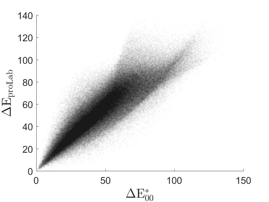
In Fig. 9, we visualize colour non-uniformities with joint distributions of Euclidian distances $\mathrm{\Delta E_{\Phi}}$ and CIEDE2000 colour differences $\mathrm{{\Delta E}^{*}_{00}}$ over test sample $G^{2}_{n_{2}}$ for each colour coordinate space. On such scatter plots, the thinner the cluster along the line passing through $\boldsymbol{\mathbf{0}}$, the more perceptually uniform the colour coordinate space is. CAM16-UCS and proLab joint distributions have significantly better shapes than those of the other colour coordinate spaces, but proLab is inferior to CAM16-UCS in the middle range distances. Note that in a region of large Euclidean distances, CAM16-UCS has two distinctly different loci in such region, which means there is significant non-uniformity in this range. Strongly decorrelated regions similar in location and shape are observed in proLab and CIELAB; however, for CIELAB the region is larger and deviates more and farther from the main locus.

To provide detailed visualization of noise heteroscedasticity, we plot charts similar to MacAdam ellipses (Fig. 10). For a set of colours from the sRGB gamut, we model the noise distributions of measurements according to the parameters of the model (52). Each distribution is projected onto the given colour coordinate space and visualized with its averaged colour. The three-dimensional structure of noise parameters is visualized by plotting the lighter colours over the dark ones.

A key feature of the proLab design is its projectivity. Within this colour coordinate space, the central projection on any plane bypassing $\boldsymbol{\mathbf{0}}$ is a chromaticity diagram, since proLab does not shift the coordinate origin. That is, colours that differ only in brightness in the original space of spectral irradiance are mapped into a single point.

Another interesting property of proLab concerns image shot noise. In a noisy image, colour estimation by arithmetic averaging is valid only in linear colour spaces. However, chromaticity estimation by linear regression is invalid even in a linear space, since the amplitude of shot noise depends on the value of the colour coordinates. But in proLab, the linear regression procedure appears to be more correct, due to the noise being more homoscedastic compared to standard linear spaces.

In this work, proLab was constructed for the D65 light source, so the question arises of how to adapt these colour coordinates to a different kind of illumination. In order to achieve the best possible accuracy, we should form sample $G^{2}_{n_{1}}$ of colour pairs over the given light source gamut, and then optimize matrix $Q$ on this sample. But such a procedure is inconvenient and time-consuming, so we suggest using an approach similar to CIELAB: parametrization of the transformation with the light source coordinates, while ‘the kernel’ of the transformation $Q$ is kept the same. We find such an approach to be optimal for proLab as well as for CIELAB, since for both systems the inaccuracy in uniformity is too significant to be fixed by a separate optimization. That is why for light sources other than D65, we suggest using the same elements of the matrix $Q$ as in (44).

For both techniques, the matrix $P$ is finally defined in accordance with the von Kries adaptation model (9). Here we use this simplification just for compatibility with existing solutions, taking into account that the given model is criticized for poor accuracy. Currently, several more accurate adaptation models also named after von Kries are known, which are expressed via linear transformation of colour coordinates [60]. Such models could also be used in proLab, since the replacement of the adaptation model by another linear (and even projective) one does not affect matrix $Q$, and requires only redefinition of matrix $N$.

Depending on the specific task, the metric parameters of proLab could also be modified. Particularly, it is not obvious that pairs with different colour differences ${\Delta E}^{*}_{00}$ should be equally weighted while solving the optimization problem. In some possible applications large (or small) colour differences could be negligible. In such cases, proLab parameters must be optimized with the same method but on a different $G^{2}_{n_{1}}$ sample.

Besides this, the relationship of the $L^{+}$ axis with brightness can be weakened in order to increase or toughen the perceptual uniformity of the result. Alternatively, the condition (22) could be more strict for LMS colour coordinates. Note that the fulfilment of requirement (22) directly implies the fulfilment of similar requirements on the linRGB coordinates. All elements of transition matrix from linRGB to CIE XYZ are non-negative, and

i.e., a non-negative increment in linRGB implies a non-negative increment in CIE XYZ. Since the transformation from sRGB to linRGB is component-wise monotonic, the aforesaid also implies that the lightness component is non-decreasing when increasing the sRGB coordinates. However, in LMS space the same behaviour is not guaranteed as the transformation matrix from LMS to CIE XYZ contains negative elements.

It is important to further study the parameters of noise in various spaces, including proLab. Our interest is focused on the experimental data for various cameras as well as on analytical models for estimation of heteroscedasticity under various conditions. Along with shot noise, these models could also consider sensor signal discreteness. Outside the context of uniform colour spaces, the effects of colour digitization in technical systems have already been studied in [61].

We also note that the secondary locus of the joint distance chart shown in Fig. 9 raises the question about the localization of the significantly non-projective parts of the gamut. On the other hand, the strict requirement of projectivity was introduced formally. In practice, the regression errors caused by the non-projectivity of the model may turn out to be insignificant compared to the noise. Therefore, further study could also involve the construction of a low-parametric and computationally simple colour model close to the projective one and with better perceptual uniformity, as well as reduced noise heteroscedasticity.

ProLab is a novel colour coordinate system that is demonstrated to be superior to CIELAB in perceptual uniformity while still preserving colour manifold linearity. This property is not present in either CIELAB or CAM16-UCS. Reproduction angular errors can be used in proLab, as in linear colour spaces. ProLab, by design, aligns angular errors of different hues to CIEDE2000 perceptual colour differences unlike the previously mentioned systems. Further, we demonstrate that image noise in proLab is more homoscedastic than in other standard spaces, including linear ones. These advantages make proLab a preferred coordinate system in which to perform structural analysis of colour distributions. Because the incidence of linear manifolds is preserved, light source direction can be estimated by the intersection of planes formed by the colour distribution of glossy surfaces in proLab. Estimating manifold coordinates with no additional corrections of noise heteroscedasticity should deliver the same or better accuracy when compared to standard linear spaces. Furthermore, the mutual positions of manifolds, including angles between lines, in proLab are in correspondence with human perception.

The MatLab/Octave implementation is available at https://github.com/konovalenko-iitp/proLab.

We would like to thank Prof. Valentina Bozhkova, our colleagues at the 25th Symposium of the International Colour Vision Society, and our colleagues at Huawei Color Constancy & Multispectral Processing Workshop 2019 for the fruitful discussions of the main idea behind this work.

References

- [1] H. Grassmann, “Zur theorie der farbenmischung,” Annalen der Physik, vol. 165, no. 5, pp. 69–84, 1853, (In German).
- [2] T. Smith and J. Guild, “The c.i.e. colorimetric standards and their use,” Transactions of the Optical Society, vol. 33, no. 3, pp. 73–134, 1931.
- [3] M. D. Fairchild, Color appearance models. John Wiley & Sons, 2013.
- [4] M. R. Luo, CIE Chromatic Adaptation; Comparison of von Kries, CIELAB, CMCCAT97 and CAT02. Springer Berlin Heidelberg, 2014, pp. 1–8.
- [5] R. S. Hunter, “Accuracy, precision, and stability of new photoelectric color-difference meter,” J. Opt. Soc. Am., vol. 38, no. 12, pp. 1094–1094, 1948.
- [6] T. I. C. on Illumination, “Technical note: Brussels session of the international commission on illumination,” J. Opt. Soc. Am., vol. 50, no. 1, pp. 89–90, 1960.
- [7] G. Wyszecki, “Proposal for a new color-difference formula,” J. Opt. Soc. Am., vol. 53, no. 11, pp. 1318–1319, 1963.
- [8] K. McLaren, “XIII—the development of the CIE 1976 (L* a* b*) uniform colour space and colour-difference formula,” Journal of the Society of Dyers and Colourists, vol. 92, no. 9, pp. 338–341, 1976.
- [9] R. G. Kuehni, “Towards an improved uniform color space,” Color Research & Application, vol. 24, no. 4, pp. 253–265, 1999.
- [10] D. H. Alman, R. Berns, H. Komatsubara, W. Li, M. R. Luo, M. Melgosa, J. H. Nobbs, B. Rigg, A. R. Robertson, and K. Witt, “Improvement to industrial colour-difference evaluation,” Central Bureau of the International Commission on Illumination, Vienna, Tech. Rep. “Publication CIE 142-2001”, 2001.
- [11] M. R. Luo, G. Cui, and B. Rigg, “The development of the cie 2000 colour-difference formula: Ciede2000,” Color Research & Application, vol. 26, no. 5, pp. 340–350, 2001.
- [12] H. Wang, G. Cui, M. R. Luo, and H. Xu, “Evaluation of colour-difference formulae for different colour-difference magnitudes,” Color Research & Application, vol. 37, no. 5, pp. 316–325, 2012.
- [13] C. Li, Z. Li, Z. Wang, Y. Xu, M. R. Luo, G. Cui, M. Melgosa, M. H. Brill, and M. Pointer, “Comprehensive color solutions: Cam16, cat16, and cam16-ucs,” Color Research & Application, vol. 42, no. 6, pp. 703–718, 2017.
- [14] H. Can Karaimer and M. S. Brown, “Improving color reproduction accuracy on cameras,” in 2018 IEEE/CVF Conference on Computer Vision and Pattern Recognition, 2018, pp. 6440–6449.
- [15] G. Hong, M. R. Luo, and P. A. Rhodes, “A study of digital camera colorimetric characterization based on polynomial modeling,” Color Research & Application, vol. 26, no. 1, pp. 76–84, 2001.
- [16] G. D. Finlayson, M. Mackiewicz, and A. Hurlbert, “Color correction using root-polynomial regression,” IEEE Transactions on Image Processing, vol. 24, no. 5, pp. 1460–1470, 2015.
- [17] S. Bianco, A. R. Bruna, F. Naccari, and R. Schettini, “Color correction pipeline optimization for digital cameras,” Journal of Electronic Imaging, vol. 22, no. 2, pp. 1–11, 2013.
- [18] A. Kordecki, “Practical testing of irradiance-independent camera color calibration,” in Proc. SPIE 11041, Eleventh International Conference on Machine Vision (ICMV 2018), vol. 11041, 2019, pp. 340–345.
- [19] J. Vazquez-Corral, D. Connah, and M. Bertalmío, “Perceptual color characterization of cameras,” Sensors, vol. 14, no. 12, pp. 23 205–23 229, 2014.
- [20] S. A. Shafer, “Using color to separate reflection components,” Color Research & Application, vol. 10, no. 4, pp. 210–218, 1985.
- [21] P. P. Nikolaev, “Some algorithms for surface color recognition,” in Simulation of learning and behavior. Nauka, 1975, pp. 121–151, (In Russian).
- [22] M. H. Brill, “Image segmentation by object color: a unifying framework and connection to color constancy,” J. Opt. Soc. Am. A, vol. 7, no. 10, pp. 2041–2047, 1990.
- [23] D. P. Nikolaev and P. P. Nikolayev, “Linear color segmentation and its implementation,” Computer Vision and Image Understanding, vol. 94, no. 1, pp. 115–139, 2004, special Issue: Colour for Image Indexing and Retrieval.
- [24] G. J. Klinker, S. A. Shafer, and T. Kanade, “Image segmentation and reflection analysis through color,” in Proc. SPIE 0937, Applications of Artificial Intelligence VI, vol. 0937, 1988, pp. 229 – 244.
- [25] H. D. Cheng, X. H. Jiang, Y. Sun, and J. Wang, “Color image segmentation: advances and prospects,” Pattern recognition, vol. 34, no. 12, pp. 2259–2281, 2001.
- [26] Y. V. Vinogradova, D. P. Nikolaev, and D. G. Slugin, “Image segmentation of color documents using color clustering,” Journal of Information Technologies and Computing Systems, vol. 2, pp. 40–49, 2015, (In Russian).
- [27] H.-C. Lee, “Method for computing the scene-illuminant chromaticity from specular highlights,” J. Opt. Soc. Am. A, vol. 3, no. 10, pp. 1694–1699, 1986.
- [28] J. Toro and B. Funt, “A multilinear constraint on dichromatic planes for illumination estimation,” IEEE Transactions on Image Processing, vol. 16, no. 1, pp. 92–97, 2007.
- [29] J. Toro, “Dichromatic illumination estimation without pre-segmentation,” Pattern Recognition Letters, vol. 29, no. 7, pp. 871–877, 2008.
- [30] S. Woo, S. Lee, J. Yoo, and J. Kim, “Improving color constancy in an ambient light environment using the phong reflection model,” IEEE Transactions on Image Processing, vol. 27, no. 4, pp. 1862–1877, 2018.
- [31] T. Zickler, S. P. Mallick, D. J. Kriegman, and P. N. Belhumeur, “Color subspaces as photometric invariants,” International Journal of Computer Vision, vol. 79, no. 1, pp. 13–30, 2008.
- [32] A. V. Nikonorov, “Spectrum shape elements model for correction of multichannel images,” Computer Optics, vol. 38, no. 2, pp. 304–313, 2014, (In Russian).
- [33] G. D. Finlayson, B. V. Funt, and K. Barnard, “Color constancy under varying illumination,” in Proceedings of IEEE International Conference on Computer Vision, 1995, pp. 720–725.
- [34] A. Gijsenij, T. Gevers, and J. Van De Weijer, “Computational color constancy: Survey and experiments,” IEEE Transactions on Image Processing, vol. 20, no. 9, pp. 2475–2489, 2011.
- [35] G. Hemrit, G. D. Finlayson, A. Gijsenij, P. Gehler, S. Bianco, B. Funt, M. Drew, and L. Shi, “Rehabilitating the colorchecker dataset for illuminant estimation,” in 26th Color and Imaging Conference Final Program and Proceedings, 2018, pp. 350–353.
- [36] G. D. Finlayson and R. Zakizadeh, “Reproduction angular error: An improved performance metric for illuminant estimation,” in Proceedings of British Machine Vision Conference, 2014, pp. 1–11.
- [37] J. Bernd, Digital Image Processing, 6th ed. Springer, 2005.
- [38] J. Liang, K. Xiao, M. R. Pointer, X. Wan, and C. Li, “Spectra estimation from raw camera responses based on adaptive local-weighted linear regression,” Optics express, vol. 27, no. 4, pp. 5165–5180, 2019.
- [39] G. Finlayson, H. Gong, and R. B. Fisher, “Color homography: theory and applications,” IEEE transactions on pattern analysis and machine intelligence, vol. 41, no. 1, pp. 20–33, 2019.
- [40] D. L. MacAdam, “Projective transformations of i. c. i. color specifications,” J. Opt. Soc. Am., vol. 27, no. 8, pp. 294–299, 1937.
- [41] G. Wallace, H. Chen, and K. Li, “Color gamut matching for tiled display walls,” in EGVE ’03: Proceedings of the workshop on Virtual environments 2003, 2003, pp. 293–302.
- [42] H. Gong, G. D. Finlayson, R. B. Fisher, and F. Fang, “3D color homography model for photo-realistic color transfer re-coding,” The Visual Computer, vol. 35, no. 3, pp. 323–333, 2019.
- [43] A. Smagina, V. P. Bozhkova, S. Gladilin, and D. Nikolaev, “Linear colour segmentation revisited,” in Proc. SPIE 11041, Eleventh International Conference on Machine Vision (ICMV 2018), vol. 11041, 2019, pp. 107–119.
- [44] I. Konovalenko, A. Smagina, V. Kokhan, and D. Nikolaev, “Prolab: perceptually uniform projective colour coordinates system,” in The 25th Symposium of the International Colour Vision Society. Abstract Book, 2019, p. 70.
- [45] P. J. Besl and N. D. McKay, “A method for registration of 3-d shapes,” IEEE Trans. Pattern Anal. Mach. Intell., vol. 14, no. 2, pp. 239–256, 1992.
- [46] J. B. Kruskal, “Multidimensional scaling by optimizing goodness of fit to a nonmetric hypothesis,” Psychometrika, vol. 29, no. 1, pp. 1–27, 1964.
- [47] P. A. García, R. Huertas, M. Melgosa, and G. Cui, “Measurement of the relationship between perceived and computed color differences,” J. Opt. Soc. Am. A, vol. 24, no. 7, pp. 1823–1829, 2007.
- [48] Q. Pan and S. Westland, “Comparative evaluation of color differences between color palettes,” in 26th Color and Imaging Conference Final Program and Proceedings, 2018, pp. 110–115.
- [49] K. Thomsen, “A euclidean color space in high agreement with the cie94 color difference formula,” Color Research & Application, vol. 25, no. 1, pp. 64–65, 2000.
- [50] P. Urban, M. R. Rosen, R. S. Berns, and D. Schleicher, “Embedding non-euclidean color spaces into euclidean color spaces with minimal isometric disagreement,” J. Opt. Soc. Am. A, vol. 24, no. 6, pp. 1516–1528, 2007.
- [51] V. V. Maximov, Transformation of colour under the changing illumination. Nauka, 1984, (In Russian).
- [52] T. Bäck, D. B. Fogel, and Z. Michalewicz, Handbook of Evolutionary Computation, 1st ed. IOP Publishing Ltd., 1997.
- [53] G. Sharma, W. Wu, and E. N. Dalal, “The ciede2000 color-difference formula: Implementation notes, supplementary test data, and mathematical observations,” Color Research & Application, vol. 30, no. 1, pp. 21–30, 2005.
- [54] R. Martí, J. A. Lozano, A. Mendiburu, and L. Hernando, Multi-start methods. Springer International Publishing, 2018, pp. 155–175.
- [55] J. Nocedal and S. J. Wright, Numerical optimization. Springer, 2006.
- [56] N. Ohta and A. R. Robertson, CIE Standard Colorimetric System. John Wiley & Sons, Ltd, 2006, ch. 3, pp. 63–114.
- [57] A. Smagina, E. Ershov, and A. Grigoryev, “Multiple light source dataset for colour research,” in Proc. SPIE 11433, Twelfth International Conference on Machine Vision (ICMV 2019), vol. 11433, 2020, pp. 635–642.
- [58] M. Stokes, M. Anderson, S. Chandrasekar, and R. Motta, “A standard default color space for the internet – srgb, version 1.10,” International Color Consortium, Tech. Rep., 1996. [Online]. Available: http://www.color.org/sRGB.xalter
- [59] D. L. MacAdam, “Visual sensitivities to color differences in daylight,” J. Opt. Soc. Am., vol. 32, no. 5, pp. 247–274, 1942.
- [60] S. Bianco and R. Schettini, “Two new von kries based chromatic adaptation transforms found by numerical optimization,” Color Research & Application, vol. 35, no. 3, pp. 184–192, 2010.
- [61] I. G. Palchikova, E. S. Smirnov, and E. I. Palchikov, “Quantization noise as a determinant for color thresholds in machine vision,” J. Opt. Soc. Am. A, vol. 35, no. 4, pp. B214–B222, 2018.
![[Uncaptioned image]](2012.07653v2/a1.jpg) |
Ivan A. Konovalenko (ORCID: 0000-0001-5705-4438) was born in Karasuk, Novosibirsk region, USSR in 1990. He received the B.S. and M.S. degrees in applied mathematics and physics from the Moscow Institute of Physics and Technology, Dolgoprudny, Russia, in 2014. From 2009 to 2013, he was a Trainee Researcher with the Predictive Modeling and Optimization Laboratory, Institute for Information Transmission Problems (IITP) of the Russian Academy of Sciences. Since 2013, he has been an Researcher with the Vision Systems Laboratory, IITP. He is the author of more than 60 articles. His research interests include computer vision, colorimetry, projective geometry and mathematical optimization. |
![[Uncaptioned image]](2012.07653v2/a2.jpg) |
Anna A. Smagina (ORCID: 0000-0002-0135-9280) received the B.S. degree in applied math and physics from Samara State Aerospace Univeristy, Russia, in 2013, and the M.S. degree in high energy physics from Moscow Institute of Physics and Technology, Russia in 2016. From 2017, she has been working as researcher in the Vision Systems Laboratory, Institute for Information Transmission Problems, Russian Academy of Sciences (Kharkevich Institute), Moscow. Author of more than 30 articles. Research interests include technical colour vision and 3D computer vision. |
![[Uncaptioned image]](2012.07653v2/a3.jpg) |
Dmitry P. Nikolaev (ORCID: 0000-0001-5560-7668) (Member, IEEE) was born in Moscow, Russia, in 1978. He received the master’s degree in physics and the Ph.D. degree in computer science from Moscow State University, Moscow, Russia, in 2000 and 2004, respectively. Since 2007, he has been the Head of the Vision Systems Laboratory, Institute for Information Transmission Problems, Russian Academy of Sciences (Kharkevich Institute), Moscow, and he has been the CTO of Smart Engines Service LLC, Moscow, since 2016. Since 2016, he has been an Associate Professor with the Moscow Institute of Physics and Technology (State University), Moscow, teaching the Image Processing and Analysis Course. He has authored over 250 scientic publications and 10 patents. His research activities are in the area of computer vision with primary application to color image understanding. Dr. Nikolaev led a team of authors to win the Document Image Binarization Competition (DIBCO), in 2017. |
![[Uncaptioned image]](2012.07653v2/a4.jpg) |
Petr P. Nikolaev (ORCID: 0000-0003-3016-3903) has a degree of Full Doctor of Phys. and Math. Sciences, awarded in 1993 in field of biophysics. He was graduated in Moscow State University in 1966 majoring in physics and got a Ph.D. degree in 1975. At present he has a tenured post of Head Researcher of Vision Systems Laboratory, Institute for Information Transmission Problems, Russian Academy of Sciences (Kharkevich Institute), Moscow and works on the theoretical problems of color and space perception, recognition and 3D representation. His major scientific achievements are related to the fundamental aspects of psychophysics of human vision, pattern recognition and image analysis. Since 2015, he has been an Professor with the Moscow Institute of Physics and Technology (State University), Moscow, teaching the Computer Vision Course. He has authored over 100 scientic publications and 3 books. Prof. Nikolaev is a Laureate of the national award “Russia’s outstanding scientist”. |