Best Arm Identification in Graphical Bilinear Bandits
Abstract
We introduce a new graphical bilinear bandit problem where a learner (or a central entity) allocates arms to the nodes of a graph and observes for each edge a noisy bilinear reward representing the interaction between the two end nodes. We study the best arm identification problem in which the learner wants to find the graph allocation maximizing the sum of the bilinear rewards. By efficiently exploiting the geometry of this bandit problem, we propose a decentralized allocation strategy based on random sampling with theoretical guarantees. In particular, we characterize the influence of the graph structure (e.g. star, complete or circle) on the convergence rate and propose empirical experiments that confirm this dependency.
Keywords:
Machine Learning, ICML1 Introduction
In many multi-agent systems the contribution of an agent to a common team objective is impacted by the behavior of the other agents. The agents must coordinate (or be coordinated) to achieve the best team performance. Consider, for instance, the problem of configuring antennas of a wireless cellular network to obtain the best signal quality over the whole network (Siomina et al., 2006). The signal quality of the region covered by a given antenna might be degraded by the behavior of its neighboring antennas due to an increase of interferences or bad user handovers. Another example is the adjustment of the turbine blades of a wind farm where the best adjustment for one turbine may generate turbulence for its neighboring turbines and thus be suboptimal for the global wind farm objective (Bargiacchi et al., 2018).
These real-life problems can be viewed as instances of a stochastic multi-agent multi-armed bandit problem (Robbins, 1952; Bargiacchi et al., 2018) where a learner (or a central entity) sequentially pulls a joint arm, one arm for each agent (e.g., all the configuration parameters of the antennas), and receives an associated global noisy reward (e.g., the signal quality over the whole network). The goal of the learner can either be to maximize the accumulated reward, implying a trade-off between exploration and exploitation, or to find the joint arm maximizing the reward, known as pure exploration or best arm identification (Bubeck et al., 2009; Audibert and Bubeck, 2010).
In this paper we focus on the best arm identification problem in a multi-agent system for which we assume the knowledge of a coordination graph representing the agent interactions (Guestrin et al., 2002).
At each round , a learner
- 1.
chooses for each node an arm in an finite arm set ,
- 2.
observes for each edge a bilinear reward .
Here, we denote by the unknown parameter matrix, and a zero-mean -sub-Gaussian random variable for all edges and round .
The goal of the central entity is to find, within a minimum number of rounds, the joint arm such that the expected global reward is maximized.
The reward reflects the quality of the interaction between the neighboring nodes and when pulling respectively the arm and at time . For instance, when configuring handover parameters of a wireless network, can be any criterion assessing the handover quality between antenna and antenna , the parameters selected by each antenna both impacting this quantity. The bilinear setting appears as a natural extension of the commonly studied linear setting to model the interaction between two agents. Furthermore, instead of a global reward being a sum of independent linear agent rewards, the global reward is now the result of the interactions between neighboring agents.
As exposed in Jun et al., 2019, the bilinear reward can be written as a linear reward in a higher dimensional space:
| (1) |
where for any matrix , denotes the vector in which is the concatenation of all the columns of .
Since the unknown parameter is common to all the edges of the graph, the expected global reward at time can also be written as the scalar product . Hence, solving the best arm identification problem in the described graphical bilinear bandit boils down to solving the same problem in a global linear bandit. Although this trick allows to use classical algorithms in linear bandits, the number of joint arms is growing exponentially with the number of nodes, making such methods impractical.
Another possible way to address this problem based on equation (1) is to consider one linear bandit per edge, with constraints between edges. For more clarity, let us define the arm set , and let us refer to any as an edge-arm and to any as an node-arm. At each round , the learner chooses for each edge an edge-arm in with the constraint that for any pair of edges and , if the edge-arm is assigned to the edge and the edge-arm is assigned to the edge , then it must be that .
Given this constraint, how do we choose the appropriate sequence of edge-arms in order to build a good estimate of ? Moreover, assuming we have built such a good estimator, is there a tractable algorithm to identify the best joint arm, or at least to find a joint arm yielding a high expected reward? In this paper, we answer these questions and provide algorithms and theoretical guarantees.
We show that even with a perfect estimator , identifying the best joint arm is NP-Hard. To address this issue, we design a polynomial time twofold algorithm. Given , it first identifies the best edge-arm maximizing . Then, it allocates to a carefully chosen subset of edges. We show that this yields a good approximation ratio in Section 4.
To build our estimator , we rely on the G-Allocation strategy, as in Soare et al., 2014. We show that there exists a sampling procedure over the node-arms such that the associated edge-arms follow the optimal G-allocation strategy developed in the linear bandit literature. This procedure allows us to avoid the difficulty of having to satisfy the edge-arm constraints explicitly. Furthermore, we analyze the sample complexity of this method. This is detailed in Section 5.
In addition, we highlight the impact of the graph structure in Section 6 and provide the explicit repercussion on the convergence rate of the algorithm for different types: star, complete, circle and matching graphs. In particular, we show that for favorable graph structures (e.g. circles), our convergence rate matches that of standard linear bandits. Finally, Section 7 evidences the theoretical findings on numerical experiments.
2 Related Work
Best arm identification in linear bandits. There exists a vast literature on the problem of best arm identification in linear bandits (Soare et al., 2014; Xu et al., 2018; Degenne et al., 2020; Kazerouni and Wein, 2019; Zaki et al., 2020; Jedra and Proutiere, 2020), would it be by using greedy strategies (Soare et al., 2014), rounding procedures (Fiez et al., 2019) or random sampling (Tao et al., 2018). Although our problem can be formulated as a linear bandit problem, none of the existing methods would scale-up with the number of agents. Nevertheless, we will be relying on classical techniques, and more specifically those developed in Soare et al., 2014.
Bilinear bandits. Bandits with bilinear rewards have been studied in Jun et al., 2019. The authors derived a no-regret algorithm based on Optimism in the Face of Uncertainty Linear bandit (OFUL) (Abbasi-Yadkori et al., 2011), using the fact that a bilinear reward can be expressed as a linear reward in higher dimension. Our work extends their setting by considering a set of dependent bilinear bandits. Besides, the goal here is to find the best arm rather than minimizing the regret.
Bandits and graphs. Graphs are often used to bring structure to a bandit problem. In Valko et al., 2014 and Mannor and Shamir, 2011, the arms are the nodes of a graph and pulling an arm gives information on the rewards of the neighboring arms. The reader can also refer to Valko, 2020 for an account on such problems. In Cesa-Bianchi et al., 2013 each node is an instance of a linear bandit and the neighboring nodes are assumed to have similar unknown regression coefficients. The main difference with our setting is that the rewards of the nodes are independent.
Combinatorial and multi-agent bandits. Allocating arms to each node of a graph to then observe a global reward is a combinatorial bandit problem (Cesa-Bianchi and Lugosi, 2012), the number of joint arms scaling exponentially with the number of nodes. This has been extensively studied both in the regret-based (Chen et al., 2013; Perrault et al., 2020) and the pure exploration context (Chen et al., 2014; Cao and Krishnamurthy, 2019; Jourdan et al., 2021; Du et al., 2020). Our problem is closer to the one presented in Amin et al., 2011 and Bargiacchi et al., 2018, where several agents want to maximize a global team reward that can be decomposed into a sum of observable local rewards as in a semi-bandit game (Audibert et al., 2011; Chen et al., 2013). However, we study a more structured context as we assume observable bilinear rewards for each edge of the graph. Furthermore, note that our problem can be solved by the algorithm presented in Du et al., 2020 with a sample complexity increasing in the number of nodes. On the contrary, we propose in this paper an algorithm with a sample complexity decreasing in the number of nodes exploiting the structure of the bilinear reward and the graph. Finally, most of the algorithms developed for combinatorial bandits assume the availability of an oracle to solve the combinatorial optimization problem returning the arm to play or the final best arm recommendation. We make no such assumption.
3 Preliminaries and Notations
Let be a directed graph with the set of nodes, the set of edges where we assume that if then , and the set containing the neighbors of a node . We denote by the number of nodes and the number of edges. We define the graphical bilinear bandit on the graph as the setting where a learner sequentially pulls at each round a joint arm , also called graph allocation or simply allocation when it is clear from the context, and then receives a bilinear reward for each edge . At each round, the joint arm can be constructed simultaneously or sequentially, however all the bilinear rewards are only revealed after the joint arm has been pulled.
We denote the number of node-arms and it is assumed that spans . For each round of the learning procedure and each node , represents the node-arm allocated to the node . For each edge , we denote the associated chosen edge-arm.
The goal is to derive an algorithm that minimizes the number of pulled joint arms required to find the one maximizing the sum of the associated expected bilinear rewards, for a given confidence level. For the sake of simplicity, we assume that the unknown parameter matrix in the bilinear reward is symmetric. We provide an analysis of the non-symmetric case in Appendix E.
For any finite set , denotes the simplex in . For any vector , will denote the -norm of . For any square matrix , we denote by the spectral norm of . Finally, for any vector and a symmetric positive-definite matrix , we define .
4 An NP-Hard Problem
In this section, we address the problem of finding the best joint arm given or a good estimator . If the best edge-arm is composed of a single node-arm , that is , then finding the best joint arm is trivial and the solution is to assign to all nodes. Conversely, if is composed of two distinct node-arms , the problem is harder.
The following theorem states that, even with the knowledge of the true parameter , identifying the best join-arm is NP-Hard with respect to the number of nodes .
Theorem 4.1.
Consider a given matrix and a finite arm set . Unless P=NP, there is no polynomial time algorithm guaranteed to find the optimal solution of
The proof of this theorem is in Appendix A and relies on a reduction to the Max-Cut problem. Hence, no matter which estimate of one can build, the learner is not guaranteed to find in polynomial time the joint arm maximizing the expected global reward. However, one can notice that, given the matrix or even a good enough estimate , identifying the edge-arm that maximizes the reward requires only reward estimations (we simply estimate all the linear reward associated to each edge-arm in ). Thus, instead of looking for the best joint arm explicitely, we will first identify the best edge-arm , and then allocate to the largest number of edges in the graph. We will also show that this approach gives a guarantee on its associated global reward.
Let us consider the graph allocation that places the maximum number of edge-arms in . It is easy to show that the subgraph containing only the edges where has been pulled is the largest bipartite subgraph included in . Recall that a graph is a bipartite if and only if one can partition the node set such that
Notice, that if is the largest bipartite subgraph in , the number of edges in is the maximal number of edge-arms that can be allocated with a single graph allocation.
Hence, finding the joint arm with the largest number of edge-arms allocated in the graph is equivalent to finding the largest bipartite subgraph in . Once that subgraph is determined, we just need to allocate to all the nodes in the node-arm and to all the nodes of the node-arm (which is equivalent to allocating to all the edges in the edge-arm ).
Furthermore, we know that every -edge graph contains a bipartite subgraph of at least edges (Erdos, 1975). Therefore, we propose Algorithm 1 which iteratively constructs a bipartite subgraph and allocates the nodes accordingly to create at least edge-arms .
Input :
, ,
Find
Set ,
for in do
The following result gives the guarantee on the global reward associated to the joint arm returned by Algorithm 1. We refer the reader to Appendix A for the proof.
Theorem 4.2.
Let us consider the graph , a finite arm set and the matrix given as input to Algorithm 1. Then, the expected global reward associated to the returned allocation verifies:
where and are respectively the highest and lowest global reward one can obtain with the appropriate joint arm. Finally, the complexity of the algorithm is in .
This type of approximation result is sometimes referred to as differential approximation or -approximation, and is often viewed as a more subtle analysis than standard approximation ratio. We emphasize that finding a better ratio than is a very hard task: such a finding would immediately yield an improved differential approximation ratio for the Max-Cut problem, which is an opened problem since 2001 (Hassin and Khuller, 2001).
5 Construction of the Estimate
In the previous section, we designed a polynomial time method that computes a -approximation to the NP-Hard problem of finding the best joint arm given . Notice that is only used to identify the best edge-arm . Thus, using an estimate of having the following property:
| (2) |
would still allow us to identify , and would thus give us the same guarantees.
In this section we tackle the problem of pulling the edge-arms during the learning procedure such that the estimated unknown parameter verifies (2) in as few iterations as possible. To do so, we first formalize the objective related to the linearized version of the problem. Then, we propose an algorithm reaching the given objective with high probability while satisfying the edge-arms constraints.
We denote by the parameter of the linearized problem and the Ordinary Least Squares (OLS) estimate of computed with all the data collected up to round . The empirical gap between two edge-arms and in is denoted .
5.1 A Constrained G-Allocation
The goal here is to define the optimal sequence that should be pulled in the first rounds so that (2) is reached as soon as possible. A natural approach is to rely on classical strategies developed for best arm identification in linear bandits. Most of the known strategies (see e.g., Soare et al., 2014; Xu et al., 2018; Fiez et al., 2019) are based on a bound of the gap error for all . This bound is then used to derive a stopping condition, indicating a sufficient number of rounds after which the OLS estimate is precise enough to ensure the identification of the best edge-arm, with high probability.
Let and let be the matrix computed with the edge-arms constructed during rounds. Following the steps of Soare et al., 2014, we can show that if there exists such that for all the following holds:
| (3) |
then with probability at least , the OLS estimate leads to the best edge-arm. Details of the derivation are given in Appendix B.
As mentioned in Soare et al., 2014, by noticing that , an admissible strategy is to pull edge-arms minimizing in order to satisfy the stopping condition as soon as possible. More formally, one wants to find the sequence of edge-arms such that:
| (G-opt-) |
This is known as G-allocation (see e.g., Pukelsheim, 2006; Soare et al., 2014) and is NP-hard to compute (Çivril and Magdon-Ismail, 2009; Welch, 1982). One way to find an approximate solution is to rely on a convex relaxation of the optimization problem (G-opt- Z ) and first compute a real-valued allocation such that
| (G-relaxed-) |
One could either use random sampling to draw edge-arms as i.i.d. samples from the distribution or rounding procedures to efficiently convert each into an integer. However, these methods do not take into account the graphical structure of the problem, and at a given round, the chosen edge-arms may result in two different assignments for the same node. Therefore, random sampling or rounding procedures cannot be straightforwardly used to select edge-arms in . Nevertheless, (G-relaxed- Z ) still gives a valuable information on the number of times, in proportion, each edge-arm must be allocated to the graph. In the next section, we present an algorithm satisfying both the proportion requirements and the graphical constraints.
5.2 Random Allocation over the Nodes
Our algorithm is based on a randomized method directly allocating node-arms to the nodes and thus avoiding the difficult task of choosing edge-arms and trying to allocate them to the graph while ensuring that every node has an unique assignment. The validity of this random allocation is based on Theorem 5.1 below showing that one can draw node-arms in and allocate them to the graph such that the associated edge-arms follow the probability distribution solution of (G-relaxed- Z ).
Theorem 5.1.
Let be a solution of the following optimization problem:
| (G-relaxed-) |
Let be defined for all by . Then, is a solution of (G-relaxed- Z ).
Sketch of proof.
The objective at the optimum in (G-relaxed- X ) and (G-relaxed- Z ) are respectively equal to and which is the dimension of their respective problem, a result known as the Equivalence Theorem (Kiefer and Wolfowitz, 1960). Thus, by multiplying the optimum value of (G-relaxed- X ) by itself, we can show that for all where with , can be written as the product . We refer to the Appendix C for the detailed proof.
This theorem implies that, at each round and each node , if is drawn from , then for all pairs of neighbors the probability distribution of the associated edge-arms follows . Moreover, as is a distribution over the node-arm set , is a joint (product) probability distribution on with marginal .
We apply the Frank-Wolfe algorithm (Frank et al., 1956) to compute the solution of (G-relaxed- X ), as it is more suited to optimization tasks on the simplex than projected gradient descent. Although we face a min-max optimization problem, we notice that the function is convex. We refer the reader to Appendix F and references therein for a proof on the convexity of and a discussion about using Frank-Wolfe for solving (G-relaxed- X ).
Given the characterization in Theorem 5.1 and our objective to verify the stopping condition in (3), we present our sampling procedure in Algorithm 2. We also note that at each round the sampling of the node-arms can be done in parallel.
Input :
graph , arm set
Set ; ; ;
Apply the Frank-Wolfe algorithm to find solution of (G-relaxed- X ).
while stopping condition (3) is not verified do
This sampling procedure implies that each edge-arm follows the optimal distribution . However, if we take the number of times each appears in the pulled edge-arms of a given round, we might notice that the observed proportion is not close to , regardless of the size of . This is due to the fact that the edge-arms are not independent because of the graph structure (cf. Section 6). Conversely, since each group of edge-arms are independent from one round to another, the proportion of each observed among the pulled edge-arms throughout rounds is close to .
One may wonder if deterministic rounding procedures could be used instead of random sampling on , as it is done in many standard linear bandit algorithms (Soare et al., 2014; Fiez et al., 2019). Applying rounding procedure on gives the number of times each node-arm should be allocated to the graph. However, it does not provide the actual allocations that the learner must choose over the rounds to optimally pull the associated edge-arms (i.e., pull edge-arms following ). Thus, although rounding procedures give a more precise number of times each node-arm should be pulled, the problem of allocating them to the graph remains open, whereas by concentration of the measure, randomized sampling methods imply that the associated edge-arms follow the optimal probability distribution . In this paper, we present a simple and standard randomized G-allocation strategy, but other more elaborated methods could be considered, as long as they include the necessary randomness.
On the choice of the G-allocation problem. We have considered the G-allocation optimization problem (G-opt- Z ), however, one could want to directly minimize , known as the XY-allocation (Soare et al., 2014; Fiez et al., 2019). Hence, one may want to construct edge-arms that follow the distribution solution of the relaxed XY-allocation problem:
Although efficient in the linear case, this approach outputs a distribution which is not a joint probability distribution of two independent random variables, and so cannot be decomposed as the product of its marginals. Hence, there is no algorithm that allocates identically and independently the nodes of the graph to create edge-arms following . Thus, we will rather deal with the upper bound given by the G-allocation as it allows sampling over the nodes.
Static design versus adaptive design. Adaptive designs as proposed for example in Soare et al., 2014 and Fiez et al., 2019 provide a strong improvement over static designs in the case of linear bandits. In our particular setting however, it is crucial to be able to adapt the edge-arms sampling rule to the node-arms, which is possible thanks to Theorem 5.1. This result requires a set of edge-arms expressed as a product of node-arms set . Extending the adaptive design of Fiez et al., 2019 to our setting would eliminate edge-arms from at each phase, without trivial guarantees that the newly obtained edge-arms set could still be derived from another node-arms set . An adaptive approach is definitely a natural and promising extension of our method, and is left for future work.
5.3 Convergence Analysis
We now prove the validity of the random sampling procedure detailed in Algorithm 2 by controlling the quality of the approximation with respect to the optimum of the G-allocation optimization problem described in (G-opt- Z ). As is usually done in the optimal design literature (see e.g., Pukelsheim, 2006; Soare et al., 2014; Sagnol, 2010) we bound the relative error :
Our analysis relies on several results from matrix concentration theory. One may refer for instance to Tropp et al., 2015 and references therein for an extended introduction on that matter. We first introduce a few additional notations.
Let be the function such that for any non-singular matrix , and for any distribution let be the associated covariance matrix. Finally let be the G-optimal design matrix constructed during rounds.
For and , let be i.i.d. random vectors in such that for all ,
Each is to be viewed as the random arm pulled at round for the node . Using this notation, the random design matrix can be defined as
One can first observe that can be bounded by the following quantity:
Hence, one needs a bound on the maximum eigenvalue of . Simple linear algebra leads to:
Thus, in addition to bounding the maximum eigenvalue of , which is equal to the minimum eigenvalue of , we need a bound on . It may be derived from concentration results on sum of random matrices derived in Tropp et al., 2015. We now state the result controlling the relative error obtained with our randomized sampling allocation. The proof can be found in the Appendix C.
Theorem 5.2.
Let be a solution of the optimization problem (G-relaxed- Z ). Let and let be such that
where and is the smallest eigenvalue of the covariance matrix. Then, at each round with probability at least , the randomized G-allocation strategy for graphical bilinear bandit in Algorithm 2 produces a matrix such that:
where
and .
We have just shown that the approximation value converges to the optimal value with a rate of . In Section 6, we show that the best case graph implies a matching the convergence rate of a linear bandit algorithm using randomized sampling to pull edge-arms without (graphical) constraints. Moreover, we will see that the worst case graph implies that .
Since we filled the gap between our constraint objective and the problem of best arm identification in linear bandits, thanks to Theorem 5.1 and 5.2, we are able to extend known results for best arm identification in linear bandits on the sample complexity and its associated lower bound.
Corollary 5.3 (Soare et al., 2014, Theorem 1).
If the G-allocation is implemented with the random strategy of Algorithm 2, resulting in an -approximation, then with probability at least , the best arm obtained with is and
where .
Moreover, let be the number of rounds sufficient for any algorithm to determine the best arm with probability at least . A lower bound on the expectation of can be obtained from the one derived for the problem of best arm identification in linear bandits (see e.g., Theorem 1 in Fiez et al., 2019):
As observed in Soare et al., 2014 this lower bound can be upper bounded, in the worst case, by which matches our bound up to log terms and the relative error .
6 Influence of the Graph Structure on
The convergence bound in Theorem 5.2 depends on . In this section, we characterize the impact of the graph structure on this quantity and, by extension, on the convergence rate. First of all, recall that
Let denote such that and let define for any random matrices and the operators and . We can derive the variance of as follows:
One can decompose the sum of the covariances into three groups: a first group where and which means that the two edges do not share any node and , and two other groups where the edges share at least one node. For all edges we consider either the edges where , yielding or the edges , yielding .
Hence, one has
Let be such that for all , and such that for all :
We want to compare the quantity for different types of graphs: star, complete, circle and a matching graph. To have a fair comparison, we want graphs that reveal the same number of rewards at each round of the learning procedure. Hence, we denote respectively , , and the number of nodes in a star, complete, circle and matching graph of edges and get:
Star graph:
Complete graph:
Circle graph:
Matching graph:
We refer the reader to Appendix D for more details on the given upper bounds. Since the star (respectively, complete, circle and matching) graph of edges has a number of nodes (respectively , and ), we obtain the bounds stated in Table 1.
| Graph | Upper bound on | |
| Star | ||
| Complete | ||
| Circle | ||
| Matching |
These four examples evidence the strong dependency of the variance on the structure of the graph. The more independent the edges are (i.e., with no common nodes), the smaller the quantity is. For a fixed number of edges , the best case is the matching graph where no edge share the same node and the worst case is the star graph where all the edges share a central node.
7 Experiments
In this section, we consider the modified version of a standard experiment introduced by Soare et al., 2014 and used in most papers on best arm identification in linear bandits (Xu et al., 2018; Tao et al., 2018; Fiez et al., 2019; Zaki et al., 2019) to evaluate the sample complexity of our algorithm on different graphs. We consider node-arms in where . This node-arm set is made of the vectors forming the canonical basis of and one additional arm with . Note that by construction, the edge-arm set contains the canonical basis of . The parameter matrix has its first coordinate equal to 2 and the others equal to 0 which makes . The best edge-arm is thus . One can note that when tends to 0, it is harder to differentiate this arm from than from the other arms. We set , for all edges and round .
We consider the two cases where which makes the edge-arms and difficult to differentiate, and which makes the edge-arm easily identifiable as the optimal edge-arm. For each of these two cases, we evaluate the influence of the graph structure, the number of edges and the edge-arm space dimension on the sampling complexity. Results are shown in Figure 1.
When , the type of the graph does not impact the number of rounds needed to verify the stopping condition. This is mainly due to the fact that the magnitude of its associated variance is negligible with respect to the number of rounds. Hence, even if we vary the number of edges or the dimension, we get the same performance for any type of graph including the matching graph. This implies that our algorithm performs as well as a linear bandit that draws edge-arms in parallel at each round. When , the number of rounds needed to verify the stopping condition is smaller and the magnitude of the variance is no longer negligible. Indeed, when the number of edges or the dimension increases, we notice that the star graph takes more times to satisfy the stopping condition. Moreover, note that the sample complexities obtained for the circle and the matching graph are similar. This observation is in line with the dependency on the variance shown in Table 1.
8 Conclusion
We introduced a new graphical bilinear bandit setting and studied the best arm identification problem with a fixed confidence. This problem being NP-Hard even with the knowledge of the true parameter matrix , we first proposed an algorithm that provides a 1/2-approximation. Then, we provided a second algorithm, based on G-allocation strategy, that uses randomized sampling over the nodes to return a good estimate that can be used instead of . Finally, we highlighted the impact of the graph structure on the convergence rate of our algorithm and validated our theoretical results with experiments. Promising extensions of the model include considering unknown parameters , different for each edge of the graph, and investigating XY-allocation strategies.
Acknowledgements
We thank anonymous reviewers, whose comments helped us improve the paper significantly.
References
- Abbasi-Yadkori et al., (2011) Abbasi-Yadkori, Y., Pál, D., and Szepesvári, C. (2011). Improved algorithms for linear stochastic bandits. In Advances in Neural Information Processing Systems, pages 2312–2320.
- Amin et al., (2011) Amin, K., Kearns, M., and Syed, U. (2011). Graphical models for bandit problems. In Proceedings of the Twenty-Seventh Conference on Uncertainty in Artificial Intelligence, page 1–10.
- Audibert and Bubeck, (2010) Audibert, J.-Y. and Bubeck, S. (2010). Best arm identification in multi-armed bandits. In Proceedings of the 23th Annual Conference on Learning Theory, pages 41–53.
- Audibert et al., (2011) Audibert, J.-Y., Bubeck, S., and Lugosi, G. (2011). Minimax policies for combinatorial prediction games. In Proceedings of the 24th Annual Conference on Learning Theory, pages 107–132.
- Bargiacchi et al., (2018) Bargiacchi, E., Verstraeten, T., Roijers, D., Nowé, A., and Hasselt, H. (2018). Learning to coordinate with coordination graphs in repeated single-stage multi-agent decision problems. In International conference on machine learning, pages 482–490.
- Bubeck et al., (2009) Bubeck, S., Munos, R., and Stoltz, G. (2009). Pure exploration in multi-armed bandits problems. In International conference on Algorithmic learning theory, pages 23–37. Springer.
- Cao and Krishnamurthy, (2019) Cao, T. and Krishnamurthy, A. (2019). Disagreement-based combinatorial pure exploration: Sample complexity bounds and an efficient algorithm. In Proceedings of the Thirty-Second Conference on Learning Theory, volume 99, pages 558–588.
- Cesa-Bianchi et al., (2013) Cesa-Bianchi, N., Gentile, C., and Zappella, G. (2013). A gang of bandits. In Advances in Neural Information Processing Systems, pages 737–745.
- Cesa-Bianchi and Lugosi, (2012) Cesa-Bianchi, N. and Lugosi, G. (2012). Combinatorial bandits. Journal of Computer and System Sciences, 78(5):1404 – 1422.
- Chen et al., (2014) Chen, S., Lin, T., King, I., Lyu, M. R., and Chen, W. (2014). Combinatorial pure exploration of multi-armed bandits. In Advances in Neural Information Processing Systems, volume 27, pages 379–387.
- Chen et al., (2013) Chen, W., Wang, Y., and Yuan, Y. (2013). Combinatorial multi-armed bandit: General framework and applications. In International Conference on Machine Learning, pages 151–159.
- Damla Ahipasaoglu et al., (2008) Damla Ahipasaoglu, S., Sun, P., and Todd, M. J. (2008). Linear convergence of a modified frank–wolfe algorithm for computing minimum-volume enclosing ellipsoids. Optimisation Methods and Software, 23(1):5–19.
- Degenne et al., (2020) Degenne, R., Ménard, P., Shang, X., and Valko, M. (2020). Gamification of pure exploration for linear bandits. arXiv preprint arXiv:2007.00953.
- Du et al., (2020) Du, Y., Kuroki, Y., and Chen, W. (2020). Combinatorial pure exploration with full-bandit or partial linear feedback. arXiv e-prints, pages arXiv–2006.
- Erdos, (1975) Erdos, P. (1975). Problems and results on finite and infinite graphs. In Recent advances in graph theory (Proc. Second Czechoslovak Sympos., Prague, 1974), pages 183–192.
- Fiez et al., (2019) Fiez, T., Jain, L., Jamieson, K. G., and Ratliff, L. (2019). Sequential experimental design for transductive linear bandits. In Advances in Neural Information Processing Systems, pages 10667–10677.
- Frank et al., (1956) Frank, M., Wolfe, P., et al. (1956). An algorithm for quadratic programming. Naval research logistics quarterly, 3(1-2):95–110.
- Guestrin et al., (2002) Guestrin, C., Lagoudakis, M. G., and Parr, R. (2002). Coordinated reinforcement learning. In Proceedings of the Nineteenth International Conference on Machine Learning, page 227–234.
- Hassin and Khuller, (2001) Hassin, R. and Khuller, S. (2001). z-approximations. Journal of Algorithms, 41(2):429–442.
- Jedra and Proutiere, (2020) Jedra, Y. and Proutiere, A. (2020). Optimal best-arm identification in linear bandits. arXiv preprint arXiv:2006.16073.
- Jourdan et al., (2021) Jourdan, M., Mutý, M., Kirschner, J., and Krause, A. (2021). Efficient pure exploration for combinatorial bandits with semi-bandit feedback. In Proceedings of the 31st International Conference on Algorithmic Learning Theory.
- Jun et al., (2019) Jun, K.-S., Willett, R., Wright, S., and Nowak, R. (2019). Bilinear bandits with low-rank structure. In International Conference on Machine Learning, pages 3163–3172.
- Kazerouni and Wein, (2019) Kazerouni, A. and Wein, L. M. (2019). Best arm identification in generalized linear bandits. arXiv preprint arXiv:1905.08224.
- Kiefer and Wolfowitz, (1960) Kiefer, J. and Wolfowitz, J. (1960). The equivalence of two extremum problems. Canadian Journal of Mathematics, 12:363–366.
- Mannor and Shamir, (2011) Mannor, S. and Shamir, O. (2011). From bandits to experts: On the value of side-observations. In Advances in Neural Information Processing Systems, pages 684–692.
- Perrault et al., (2020) Perrault, P., Boursier, E., Valko, M., and Perchet, V. (2020). Statistical efficiency of thompson sampling for combinatorial semi-bandits. In Advances in Neural Information Processing Systems.
- Petersen and Pedersen, (2012) Petersen, K. B. and Pedersen, M. S. (2012). The matrix cookbook, nov 2012. URL http://www2. imm. dtu. dk/pubdb/p. php, 3274:14.
- Pukelsheim, (2006) Pukelsheim, F. (2006). Optimal Design of Experiments. Society for Industrial and Applied Mathematics.
- Rizk et al., (2019) Rizk, G., Colin, I., Thomas, A., and Draief, M. (2019). Refined bounds for randomized experimental design. NeurIPS Workshop on Machine Learning with Guarantees.
- Robbins, (1952) Robbins, H. (1952). Some aspects of the sequential design of experiments. Bulletin of the American Mathematical Society, 58(5):527–535.
- Sagnol, (2010) Sagnol, G. (2010). Optimal design of experiments with application to the inference of traffic matrices in large networks: second order cone programming and submodularity. PhD thesis, École Nationale Supérieure des Mines de Paris.
- Siomina et al., (2006) Siomina, I., Varbrand, P., and Yuan, D. (2006). Automated optimization of service coverage and base station antenna configuration in UMTS networks. IEEE Wireless Communications, 13(6):16–25.
- Soare et al., (2014) Soare, M., Lazaric, A., and Munos, R. (2014). Best-arm identification in linear bandits. In Advances in Neural Information Processing Systems, pages 828–836.
- Tao et al., (2018) Tao, C., Blanco, S., and Zhou, Y. (2018). Best arm identification in linear bandits with linear dimension dependency. In Proceedings of the 35th International Conference on Machine Learning, volume 80, pages 4877–4886.
- Tropp et al., (2015) Tropp, J. A. et al. (2015). An introduction to matrix concentration inequalities. Foundations and Trends® in Machine Learning, 8(1-2):1–230.
- Valko, (2020) Valko, M. (2020). Bandits on graphs and structures.
- Valko et al., (2014) Valko, M., Munos, R., Kveton, B., and Kocák, T. (2014). Spectral bandits for smooth graph functions. In Xing, E. P. and Jebara, T., editors, International conference on machine learning, volume 32 of Proceedings of Machine Learning Research, pages 46–54.
- Welch, (1982) Welch, W. (1982). Algorithmic complexity: Three np-hard problems in computational statistics. Journal of Statistical Computation and Simulation - J STAT COMPUT SIM, 15:17–25.
- Xu et al., (2018) Xu, L., Honda, J., and Sugiyama, M. (2018). A fully adaptive algorithm for pure exploration in linear bandits. In Proceedings of the Twenty-First International Conference on Artificial Intelligence and Statistics, volume 84, pages 843–851.
- Zaki et al., (2019) Zaki, M., Mohan, A., and Gopalan, A. (2019). Towards optimal and efficient best arm identification in linear bandits. arXiv preprint arXiv:1911.01695.
- Zaki et al., (2020) Zaki, M., Mohan, A., and Gopalan, A. (2020). Explicit best arm identification in linear bandits using no-regret learners. arXiv preprint arXiv:2006.07562.
- Çivril and Magdon-Ismail, (2009) Çivril, A. and Magdon-Ismail, M. (2009). On selecting a maximum volume sub-matrix of a matrix and related problems. Theoretical Computer Science, 410(47):4801 – 4811.
Appendix A An NP-Hard Problem
A.1 Proof of Theorem 4.1
Theorem A.1.
Consider a given matrix and a finite arm set . Unless P=NP, there is no polynomial time algorithm guaranteed to find the optimal solution of
Proof.
We prove the statement by reduction to the Max-Cut problem. Let be a graph with . Let , where and . Let . For any joint arm assignment , let be defined as . Note that
where is the indicator function. The assignement induces a cut , and the value of the assignment is precisely twice the value of the cut. Thus, if there was a polynomial time algorithm solving our problem, this algorithm would also solve the Max-Cut problem. ∎
A.2 Proof of Theorem 4.2
Theorem A.2.
Let us consider the graph , a finite arm set and the matrix given as input to Algorithm 1. Then, the expected global reward associated to the returned allocation verifies:
where and are respectively the highest and lowest global reward one can obtain with the appropriate joint arm. Finally, the complexity of the algorithm is in .
Proof.
Given the matrix , the algorithm obtains the two node-arms solution of
Note that it is equivalent to obtain solution of
Let us analyze a round of Algorithm 1 where we assign the arm of a node in . For sake of simplicity, we assume that node is assigned at round . At round , we count the number of neighbors of that have already been assigned the arm and we count the number of neighbors of that have already been assigned the arm . Then, node is assigned the arm least represented among its neighbors, that is arm if and otherwise. Eventually, the optimal edge-arm has been assigned times among node ’s neighborhood. Hence, for each node , if we denote the sum of all the rewards obtained with the edge-arms constructed only during the round , we have
One can notice that the arm can only be equal to or . Let assume that without loss of generality and let consider the worst case where is always equal to . Since z is constructed with the same node-arm , the allocation that constructs at each edge the edge-arm exists (which is allocating to all the nodes), thus .
Moreover one can also notice that . We thus have,
Now let us sum all the rewards obtained with the constructed edge-arms at each round of the algorithm, that is the global reward of the graph allocation returned by the proposed algorithm:
Moreover, the algorithm does estimation to find the best couple , and each of the rounds of the algorithm is in . Hence the complexity is equal to . ∎
Appendix B Deriving the stopping condition
In this section, we remind key results to derive the stopping condition. We refer the reader to Soare et al., 2014 and references therein for additional details. Let be the set of edge-arms and let . For , we consider a sequence of edge-arms and the corresponding noisy rewards . We assume that the noise terms in the rewards are i.i.d., following a -sub-Gaussian distribution. Let be the solution of the ordinary least squares problem with and . We first recall the following property.
Proposition B.1 (Proposition 1 in Soare et al., 2014).
Let . For every fixed sequence , with probability , for all and for all , we have
Our goal is to find the arm that has the optimal expected reward . In other words, we want to find an arm , such that for all , . However, one does not have access to , so we have to use its empirical estimate.
Let us consider a confidence set centered at and such that , for some . Since belongs to with probability at least , one can stop pulling arms when an arm has been found, such that the above condition is verified for any . More formally, the best arm identification task will be considered successful when an arm will verify the following condition for any and any :
where is the empirical gap between and .
Using the upper bound in Proposition B.1, one way to ensure that is to define the confidence set as follows
Then, the stopping condition can be reformulated as follows:
| (4) |
Appendix C Estimation of the unknown parameter
C.1 Proof of Theorem 5.1
To prove Theorem 5.1, we first state some useful propositions and lemmas. For any finite set , we define the function as follows: for any ,
Lemma C.1.
Let be a finite set spanning and let . If is a minimizer of , then is a solution of
Proof.
First, let us notice that, for any , one has . Thus, is also a minimizer of . In addition, is spanning so . Developing yields:
where denotes the Kronecker product. We can now focus on the central term:
and the result holds. ∎
Theorem C.2.
Let be a minimizer of . Let be the distribution defined from such that, for all , . Then is a minimizer of .
Proof.
From Kiefer and Wolfowitz, 1960, we know that and . Then, using Proposition C.1, one has
This result implies that . Since , is a minimizer of .
∎
C.2 Proof of Theorem 5.2
To prove our confidence bound, we need the two following proposition. The first one is from (Tropp et al., 2015).
Proposition C.3 (Tropp et al., 2015, Chapter 5 and 6).
Let be i.i.d. positive semi-definite random matrices in , such that there exists verifying . Let be defined as . Then, for any , one can lowerbound as follows:
If in addition, there exists some , such that , then for any , one has
From the second inequality, (Rizk et al., 2019) derived a slightly different inequality that we use here :
Proposition C.4 (Rizk et al., 2019, Appendix A.3).
Let be i.i.d. random symmetric matrices in such that there exists such that , almost surely. Let . Then, for any , one has:
where .
Finally, to prove our main theorem, we need the following lemma.
Lemma C.5.
One has , where is the smallest eigenvalue of the covariance matrix .
Proof.
Define . First, for any semi-definite matrix , we have . Because is positive definite and symmetric, and by Rayleigh-Ritz theorem,
Let be the matrix whose rows are vectors of in an arbitrary order. Notice that spans , since spans . Now for any , define as a vector such that . Then,
Define . Clearly, . So we have
The last inequality comes from Kiefer and Wolfowitz equivalence theorem (Kiefer and Wolfowitz, 1960). Now observe that can be obtained by least square regression : where is the Moore-Penrose pseudo-inverse. Note that is a Gram matrix. It is known that for a matrix having singular values , its pseudo-inverse has singular values for all . So for , we have:
where refers to the smallest singular value. Let refer to the smallest eigenvalue. Noting that
yields the desired result.
∎
We are now ready to state the bound on the random sampling error, relatively to the objective value of the convex relaxation solution.
Theorem C.6.
Let be a minimizer of . Let and let be such that
where and is the smallest eigenvalue of the covariance matrix . Then, at each round , with probability at least , the randomized G-allocation strategy for graphical bilinear bandit in Algorithm 2 produces a matrix such that:
where
and .
Proof.
Let be i.i.d. random vectors in such that for all , . For and , we define the random matrix by
Finally, let us define for all , the edge-wise sum , that is
One can easily notice that are i.i.d. random matrices. We define the overall sum and our goal is to measure how close is to , where corresponds to the total number of sampled arms during the rounds of the learning procedure. By definition of , one has
This allows us to bound the relative error as follows:
Using the fact that (Kiefer and Wolfowitz, 1960), we obtain
Therefore, controlling the quantity will allow us to provide an upper bound on the relative error. Notice that
Using Proposition C.3, we know that for any , the following holds:
with probability at least . Similarly, using Proposition C.4, for any , we have
with probability at least . Combining these two results with a union bound leads to the following bound, with probability :
In order to obtain a unified bound depending on one confidence parameter , one could optimize over and , subject to . This leads to a messy result and a negligible improvement. One can use simple values , so the overall bound becomes, with probability :
This can finally be formulated as follows:
Using the obtained bound on yields
By noticing that and by using Lemma C.5, the result holds. ∎
Appendix D Variance analysis
Star graph.
The covariance matrix of the star graph can be bounded as follows:
Since the star graph of edges has a number of nodes , we have
Complete graph.
As for the star graph,
Since the complete graph of edges has a number of nodes , we have
Circle graph.
Again,
Since the circle graph of edges has a number of nodes , we have
Matching graph.
Finally,
Since the matching graph of edges has a number of nodes , we have
Appendix E Generalization
In this section, we provide some insights into the generalization to broader reward settings.
E.1 When is not symmetric
Consider the same graphical bilinear bandit setting as the one explained in the paper with the only difference that is not symmetric. We recall here that in the graph associated to the graphical bilinear bandit setting, if and only if . Hence, for a given allocation , one can write the associated expected global reward as follows :
Let us denote . One can notice that is symmetric. Solving the graphical bilinear bandit with the matrix is exactly what we propose throughout the main paper.
E.2 When the reward captures more information than the interactions between agents
Consider the real world problems introduced in the paper, but with the difference that instead of a reward only related to the interaction between two neighboring agents/nodes, there is an additional term that informs about the absolute quality of the arm chosen by the agent itself. More formally we consider the following reward for the node :
where is a second unknown parameter that allows to capture the quality of the arm chosen by the node independently of its neighbors.
In order to add a constant term in the reward, let us construct the set such that each arm is associated to a new arm defined as . Moreover, let us define the matrix as follows:
One can easily verify that for any edge and any time step , the reward can now be written as follows:
which leads to the same graphical bilinear bandit setting explained in Section 3, this time in dimension instead of . Hence, all the previous results hold for this more general graphical bilinear bandit problem, provided any dependence in is modified to .
Appendix F Computing
In Algorithm 2, we need to find the solution of . In fact we need to sample from it. We show that for any set , the function is convex and we use the Frank-Wolfe algorithm (Frank et al., 1956) to compute and . The convergence of the algorithm has been proven in Damla Ahipasaoglu et al., 2008. Note that one can only compute or to obtain the other one thanks to C.2.
Proposition F.1.
Let , for any set , is convex.
Proof.
Let be two distributions in . If either or are not invertible, then for any one has
Otherwise, for , we define the positive definite matrix as follows:
Simple linear algebra (Petersen and Pedersen, 2012) yields
Using this result and the fact that , we obtain
Therefore, for any ,
which shows convexity for any fixed . The final results yields from the fact that is a maximum over convex functions.
∎
Appendix G Additional experiment and information
We define the set of arms that is made of node-arms randomly sampled from a multivariate 5-dimensional Gaussian distribution and then normalized so that for all . In all the figures the results are averaged over 100 random repetitions of the experiments.
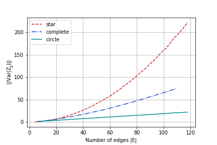
We propose to validate our insight and compute the evolution of for the three types of graphs (star, complete and circle) and different number of edges. The results are shown in Figure 2. One can notice that we retrieve the dependence of the variance for the star graph, the for the complete graph and the linear dependence for the circle graph.
Machine used for all the experiments.
Intel(R) Xeon(R) CPU E5-2667 v4 @ 3.20GHz - 24 CPUs used.