Self-testing of binary Pauli measurements requiring neither entanglement nor any dimensional restriction

It is hard to overemphasise the role of emerging quantum technology in recent times. Various real life applications, such as quantum key distribution qkd, quantum sensing qsensing, quantum metrology metrology, quantum internet internet, and machine learning mlearning have been investigated with great prospects. For such prospects to materialize in practice, it becomes utmost important to design experiments which can test whether the quantum components of the required devices function properly. To this end, various certification or verification protocols have been employed, such as those based on tomography and benchmarking bench, as well as self-testing protocols based essentially on observed statistics my'98; my'04.

Among several certification protocols generic quantum tomography is the most powerful, but at the same time it is the most resource consuming. Randomized benchmarking refers to a collection of methods that aim at reliably estimating the figure of merit of the overlap between the physical quantum process and it’s ideal counterpart. For both randomized benchmarking or quantum tomography, trusted mesurements are required in order to certify quantum devices. On the other hand, self-testing of quantum components based on statistics collected from lesser number of measurements and minimal physical assumptions, require lesser trust on the measurement devices and are experimentally more efficient and less resource consumingbench.

Self-testing based on the Bell test was proposed initially in the context of quantum cryptography my'98; my'04, where it was shown that maximum violation of the Bell-CHSH inequality Bell'64; chsh'69 implies that the underlying quantum state is maximally entangled and the local measurements performed by two distant parties are anticommuting popescu'92. In such self-testing protocols one can uniquely identify quantum states and measurements (upto some local isometries) by observing extreme correlations in measurement statistics. The underlying assumptions are the same as those required for implementation of loophole free Bell tests hensen'15; knill'15; zeilinger'15; weinfurter'17. Since then all pure bipartite entangled states and certain multipartite quantum states such as graph states have been self-tested Col; mayers2003 in this scenario. Self-testing of pure entangled bipartite states has also been investigated Supic; goswami; Goh; SBK20 employing Einstein-Podolski-Rosen steering Wiseman. Self-testing using steering is weaker in the sense that it requires more assumptions compared to that based on Bell tests, but the former is easier to verify experimentally peng.

In this regard, it is worthwhile to mention that self-testing based on maximal violation of some nonclassicality revealing criterion is very fragile as idealised situations in the laboratory are rare to occur. Therefore, a self-testing statement is useful for practical purposes if it has reasonable robustness Scarani2; Yang; Bamps; Kani2. For instance, there are robust self-testing protocols for which given a certain level of violation of a Bell inequality (but not necessarily maximal), nontrivial lower bound on the fidelity between the initially unknown state and a given target state has been shown. Robust self-testing of higher dimensional state has also been studied Scarani3; supic2018; Zhang'18. Apart from various special class of quantum states, different types of measurements including maximally incompatible observables popescu'92, entangling Bell-measurement bancal'18; renou'18, binary observables kani'17, more than two dichotomic observables Mck; Bowles'18, and non-maximally anticommuting observables Pironio have also been self-tested (See Ref.supic'19 for a review).

Apart from the above schemes of self-testing of measurements based on the use of quantum correlations in entangled states, some certification methods for self-testing have been proposed that do not require entanglement chen'11; brunner'15; bourennane'16; Tavakoli. A pair of anticommuting Pauli observables have been self-tested in the prepare and measure scenario tavakoli'18, employing the quantum advantage of $2\mapsto 1$ random access code (RAC) ambainis'99; tavakoli'15. Such approaches in the context of self-testing of local states and measurements are more resource efficient and experimentally feasible compared to schemes based on nonlocal quantum correlations since they do not require entanglement, an expensive resource. However, the assumption of an upper bound on the system-dimension has been crucial for such approaches, and hence, the verifier needs to trust the measurement devices more.

Another self-testing protocol has been constructed for three-dimensional states and measurements kishor'19 based on contextuality of quantum theory ks'67, which requires certain restrictive assumptions such as the compatibility between subsequent projective measurements supic'19. Recently, an extension of the scheme has been proposed based on the sum of sqaures decomposition of a family of non-contextual inequalities kcbs, relaxing some of the above restrictions saha'20. Self-testing of arbitrary high-dimensional local quantum systems using contextuality has also been proposed where the assumption of projective measurement is necessary kishor'19(1). The above protocols pertain to local measurements in three and above dimensions. On the other hand, among all measurements in quantum information processing, the measurements with dichotomic settings and outcomes are the most widely used ones. Hence, the design of resource efficient self-testing protocols for such meaurements with minimal assumptions is necessary for practical purposes.

In the present work, we develop a scheme of self-testing binary Pauli measurements in a hitherto unexplored scenario, i.e., employing nonclassicality of temporal correlations exhibited via violation of the Leggett-Garg inequality(LGI) LG'85; emary'14 and predictabilitykofler'13; rand'16, which does not require any entanglement. LGI has been employed to probe macroscopic coherence and to study quantum to classical transition LG'85; emary'14; LG'02; kofler'07; kofler'13; brukner'04; mal'16; mal'18; mal'19. Various aspects of temporal correlations have been investigated fritz'10; budroni'13; rand'16; bm'14; brierley'19; usha'13; alok'17; das'18; ku'18; titas'18 and experimentally realized knee'12; robens'15; knee'16; ku'19; shayan'19; spee'20. Here, we employ the violation of LGI, and invoke a minimal set of assumptions which can be easily met in a real experiment, in order to provide a self-testing statement for binary Pauli measurements without any need to restrict the dimension of the Hilbert space accessed by the quantum devices. We further perform the robustness analysis of our self-testing protocol by deriving a lower bound on the fidelity of the measured observables with that of ideal ones.

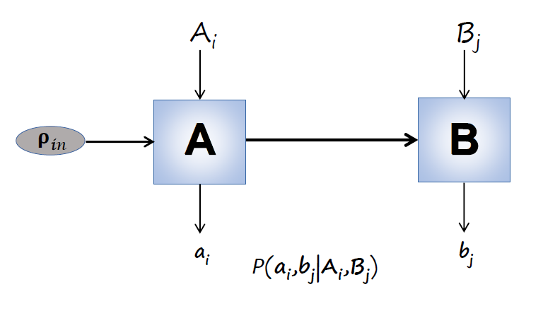
We start with a brief description of the Leggett-Garg (LG) test (Fig.-1) which enables self-testing of Pauli measurements whenever extremal correlations of LGI are observed. In a LG test, a single system is measured sequentially at different instants of time in order to obtain temporal correlations. Two sequential binary measurements are performed (by Alice and Bob, respectively) on an identical initial state prepared by the experimenter in every run of the experiment. In contrast to the sequential measurement scenario of self-testing using contextuality kishor'19, here subsequent measurements are not required to commute with each other.

Alice and Bob have two choices of binary measurements, say, $\{A_{1},A_{2}\}$ and $\{B_{1},B_{2}\}$ to perform in each run. The probability of obtaining outcome $a_{i}$ and $b_{j}$ is denoted by $P(a_{i},b_{j}\mid A_{i},B_{j})$, when Alice measures $A_{i}$ at time $t_{m}$ and Bob measures $B_{j}$ at some later instant $t_{m+1}$, with $i,j\in\{1,2\}$ and $a_{i},b_{j}\in\{0,1\}$. Let us denote, $\mathcal{P}_{a_{i}|A_{i}}$, $\mathcal{P}_{b_{j}|B_{j}}$ as projectors so that $\sum_{a_{i}}\mathcal{P}_{a_{i}|A_{i}}=\mathbb{I},\sum_{b_{j}}\mathcal{P}_{b_{j}|B_{j}}=\mathbb{I}$. The two-time joint probability can be obtained using Bayes’ rule as,

The two-time correlation is defined as,

where $\oplus$ denotes addition modulo $2$. The four-term LGI in terms of the above correlators is given by,

Any model compatible with classical theory predicts that the maximal value of the above expression is $2$, whereas the quantum theory can violate this inequality up to $2\sqrt{2}$. Suppose, in a single run, Alice performs a projective qubit measurement, $A_{1}\equiv\hat{a_{1}}.\vec{\sigma}$ (to make the preliminary discussion simple, but it can be any general measurement too) on an arbitrary input state, $\rho_{in}$ at time $t_{1}$, and Bob performs a qubit measurement, $B_{1}\equiv\hat{b_{1}}.\vec{\sigma}$ at some later time $t_{2}$, where $\hat{a_{1}}$ and $\hat{b_{1}}$ are the Bloch vectors denoting Alice’s and Bob’s measurement directions respectively and $\vec{\sigma}$ is the vector of Pauli matrices. Then the maximum quantum violation, $2\sqrt{2}$, can be achieved by the following measurement settings,

upto some local unitary. In the context of self-testing, all the four measurements are a priori unknown to Alice and Bob. Our goal is to certify above measurements from the observed statistics, under some suitable and minimal assumptions.

LGI has been earlier derived using the assumptions of non-invasive measurement and realism brukner'04; mal'16. However, those assumptions are at ontological level, and hence, cannot be verified individually. Rather a conjunction of them can be verified in an experiment. On the other hand, in rand'16, LGI was derived from some operational assumptions called predictability and no signalling in time (NSIT) kofler'13. Subsequently, the NSIT condition has been experimentally observed on a variety of input states expnsit. Here we present the essential features of the LGI derivation rand'16. Let us first state the two assumptions in precise mathematical form.

Predictability : A model is said to be predictable if the joint statistics $P(a_{i},b_{j}\mid A_{i},B_{j})\in\{0,1\}~\forall a_{i},b_{j},A_{i},B_{j}$ wiseman'12.
NSIT : NSIT is defined by the condition that measurement statistics is not influenced by the earlier measurements. Mathematically, $P(b_{j}\mid B_{j})=P(b_{j}\mid A_{i},B_{j})~\forall A_{i},B_{j},b_{j}$.
In order to derive LGI from the above two assumptions, our aim is to show that

Suppose $\lambda$ denotes some underlying variable at the ontological level, averaging over which we obtain joint probabilities observed in an experiment, i.e.,

LGI follows in a straightforward way when the joint probability at the ontological level gets factorised, or in other words, we have to show that predictability together with NSIT leads to

As further conditioning does not change the deterministic probability distribution, we have from the predictability, $P(a_{i},b_{j}\mid A_{i},B_{j},\lambda)=P(a_{i},b_{j}\mid A_{i},B_{j})$. Using Bayes’ rule one has

The condition of NSIT implies $P(b_{j}\mid A_{i},B_{j})=P(b_{j}\mid B_{j})$. Also, as physically reasonable and broadly accepted, a later measurement cannot influence the past measurement result, and hence $P(a_{i}\mid A_{i},B_{j},b_{j})=P(a_{i}\mid A_{i})$. With the above implications, one can construct a theory at the ontological level where $P(a_{i}\mid A_{i},\lambda)=P(a_{i}\mid A_{i})$, $P(b_{j}\mid B_{j},\lambda)=P(b_{j}\mid B_{j})$, which lead to Eq. (6). Now, a straightforward calculation leads us to derive the four-term LGI (3) which is bounded by $2$.

Despite some structural similarities, the LG-test is essentially different from the Bell-test clemente, and also has some loopholes which are different from that of the Bell-test wilde. The approach adopted in this paper for the derivation of LGI is based on the conjunction of Predictability and NSIT. In the present scenario it is ensured that NSIT condition is satisfied, as we see in the next section. This means that if LGI is violated, then predictability must have to be violated. Thus, the violation of predictability naturally guarantees non-classicality which is required for the purpose of self-testing.

The above derivation of LGI with the assumptions of predictability and NSIT helps us to devise a self-testing protocol for binary Pauli measurements (II) whenever extremal non-classical temporal correlations are observed. We formulate the self-testing protocol in such a way that the NSIT condition is satisfied so that maximal violation of the LGI will imply the violation of the predictability condition, and hence, no classical strategy is able to reproduce the statistics. We now make a minimal assumption which is again very natural in the sequential measurement scenario, since otherwise, a classical model may simulate the quantum violation of LGI.

Assumption : The measurement device of Alice acts only on the input state prepared by the experimenter, and the measurement device of Bob acts only on the state produced by Alice’s measurement, with both returning only the respective post-measurement states.

A similar assumption was also considered in Ref.saha'20 for the purpose of self-testing of local three dimensional measurements using the sum-of-squares decomposition of a family of non-contextual inequalities kcbs. However, in our approach using LGI we are interested here in the self-testing of binary qubit measurements. Employing the maximum violation of LGI along with NSIT condition we can self-test the binary qubit measurements given by Eq. (II) upto some local unitaries. Our self-testing protocol does not depend on the input state. However, for the sake of a formal proof of self-testing, we first consider a general qubit state (in Lemma 1). Then, making use of this proof, we extend our result for states in any dimension (Lemma 2). Our formal proof of self-testing is thus accomplished in the following two steps (lemma 1 and 2), and finally we present the proof of isometry in Theorem 1.

Lemma 1.  The maximum violation of LGI (i.e, $\mathcal{K}_{4}^{\text{max}}=2\sqrt{2}$) implies implementation of the qubit measurement observables given by equation (II) upto some local unitaries, satisfying the NSIT condition.

We now show how maximal violation of LGI can also be used to self-test the Pauli measurements even if the measurement operators act on a higher dimensional Hilbert space. Let the initial state be $\rho_{in}$ in an arbitrary dimensional Hilbert space, and the measurements $A_{i},B_{j}$ both act on this space.

Lemma 2.  The maximum violation of LGI (i.e, $\mathcal{K}_{4}^{\text{max}}=2\sqrt{2}$) implies implementation of the block diagonal measurement, i.e., $A_{1}=\oplus_{i}\sigma_{z}^{i},A_{2}=\oplus_{i}\sigma_{x}^{i},B_{1}=\oplus_{j}(\sigma_{x}^{j}+\sigma_{z}^{j})/\sqrt{2},B_{2}=\oplus_{j}(\sigma_{x}^{j}-\sigma_{z}^{j})/\sqrt{2}$.

The above two lemmas enables us to present the following theorem.

Theorem 1.  If $\mathcal{K}_{4}^{\text{max}}=2\sqrt{2}$ is observed in LG-test under Assumption 1, with the measurements of Alice, $A_{i}$ acting on $H_{d}$, producing the post measurement states $\left\{\frac{\mathcal{P}_{a_{i}|A_{i}}\rho_{in}\mathcal{P}_{a_{i}|A_{i}}^{\dagger}}{\text{Tr}\left[\mathcal{P}_{a_{i}|A_{i}}\rho_{in}\mathcal{P}_{a_{i}|A_{i}}^{\dagger}\right]}\right\}_{a}$, and the measurements of Bob $B_{j}$ acting on these post measurement states, then there exists an isometry $\Phi:\mathcal{H}^{d}\rightarrow\mathcal{C}^{2}\otimes\mathcal{H}^{d}$ such that

where $\left|\psi^{\texttt{ideal}}_{a|A_{i}}\right\rangle$ are the eigenstates of Alice’s ideal measurements and $B^{\texttt{ideal}}_{j}$ are Bob’s ideal measurements given by Eq. (4) respectively, and $\left|\texttt{junk}\right\rangle$ is a junk state acting on $\mathcal{H}^{d}$.

Robustness of self-testing of measurements is quantified as how the actual observables which are to be self-tested differ from the ideal ones. Hence, characterization of the fidelities between the real measurements and the ideal measurements is warranted. Let us first perform the robustness analysis of the measurements on Alice’s side i.e, $\left\{\mathcal{P}_{a_{i}|A_{i}}\right\}$. Given an arbitrary set of measurements $\left\{\mathcal{P}_{a_{i}|A_{i}}\right\}$, the average fidelity with the ideal measurements are,

Here $\Lambda$ is a quantum channel and the fidelities are defined as usual, $F(\rho,\sigma)=\text{Tr}(\sqrt{\sqrt{\rho}\sigma\sqrt{\rho}})$. The fidelities between the real and the ideal measurements, $F(\mathcal{P}_{a_{i}|A_{i}}^{\text{ideal}},\Lambda[\mathcal{P}_{a_{i}|A_{i}}])$ simplify to $\text{Tr}(\Lambda\left[\mathcal{P}_{a_{i}|A_{i}}\right]\mathcal{P}_{a_{i}|A_{i}}^{\text{ideal}})$. The lower bound on the smallest possible value of the average fidelity $S$, given a particular violation of the four-time LGI $\mathcal{K}_{4}$, can be found by minimizing over all sets of four measurements of $\mathcal{P}_{a_{i}|A_{i}}$,

In order to a lower bound for $\mathcal{F}$ as a function of LGI-violation $\mathcal{K}_{4}$, we use the operator inequality approach given in Refs. Kani2; tavakoli'18. Rewriting $\mathcal{K}_{4}$ in terms of an operator $W_{ia_{i}}$ and $\mathcal{P}_{a_{i}|A_{i}}$, where $W_{ia_{i}}=\frac{1}{2}[(-1)^{a_{i}}(\mathcal{P}_{B_{1}}+(-1)^{i-1}\mathcal{P}_{B_{2}})]$, $\mathcal{P}_{B_{i}}\equiv\mathcal{P}_{0|B_{i}}-\mathcal{P}_{1|B_{i}}$, we have,

Let us now define another operator $K_{ia_{i}}(\mathcal{P}_{B_{1}},\mathcal{P}_{B_{2}})\equiv\Lambda^{\dagger}(\mathcal{P}_{B_{1}},\mathcal{P}_{B_{2}})[\mathcal{P}_{a_{i}|A_{i}}^{\text{ideal}}]$. Considering an operator inequality of the form,

with $s$ and $\mu_{ia_{i}}(\mathcal{P}_{B_{1}},\mathcal{P}_{B_{2}})$ being real coeficients, the average fidelity $S$ (and hence $\mathcal{F}$) can be lower bounded as,

where $\mu\equiv 1/4~min_{\mathcal{P}_{B_{1}},\mathcal{P}_{B_{2}}}\sum_{i,a_{i}}\mu_{ia_{i}}(\mathcal{P}_{B_{1}},\mathcal{P}_{B_{2}})$.

Since we can use Jordan’s lemma to write the observables of Alice in a block-diagonal form with block of size at most $2\times 2$, it suffices for our purpose to focus on each block as in Ref. Kani2 to find the constants $s$ and $\mu$ for lower bounding the fidelity. The goal of the robustness analysis is to obtain a self-testing bound as tight as possible. Following Ref. tavakoli'18, adoption of the dephasing channel $\Lambda$, as an extraction map suffices to achieve our aim of finding an optimal self-testing bound.

where $\xi(\theta)\in[-1,1]$ and

For the interval $0\leq\theta\leq\pi/4$

and similarly $K_{20}=\frac{\mathbb{I}+\xi(\theta)\sigma_{x}}{2}$ , $K_{21}=\frac{\mathbb{I}-\xi(\theta)\sigma_{x}}{2}$, $K_{11}=\frac{\mathbb{I}-\sigma_{z}}{2}$.
whereas, for the interval $\pi/4\leq\theta\leq\pi/2$,

$K_{10}=\frac{\mathbb{I}+\xi(\theta)\sigma_{z}}{2}$,             $K_{20}=\frac{\mathbb{I}+\sigma_{x}}{2}$,

$K_{11}=\frac{\mathbb{I}-\xi(\theta)\sigma_{z}}{2}$,             $K_{21}=\frac{\mathbb{I}-\sigma_{x}}{2}$.

We can, without loss of generality, represent the two measurements in the x-z plane as,

and therefore, $W_{10}=\cos(\theta)\sigma_{z}$, $W_{20}=\sin(\theta)\sigma_{x}$, and $W_{21}=-\sin(\theta)\sigma_{x}$, $W_{11}=-\cos(\theta)\sigma_{z}$.

We analyze the operator inequality in the interval $0\leq\theta\leq\pi/4$ and $\pi/4\leq\theta\leq\pi/2$ separately. One can see that the effective number of inequalities may be reduced since there are symmetries in the expression of $K_{ia_{i}}$ and $W_{ia_{i}}$, and hence, without loss of generality we can choose $\mu_{o}\equiv\mu_{20}=\mu_{21}$ and $\mu_{e}\equiv\mu_{10}=\mu_{11}$. After simplication we get,

and,

In order to obtain the strongest bound, we have to choose the largest value of $\mu_{o}$ and $\mu_{e}$ consistant with their respective constraints, i.e., in the first interval,

A similar procedure in the second interval leads to,

The expressions in the two intervals are related to each other by the transfomations $\mu_{o}\leftrightarrow\mu_{e}$ and $\sin(\theta)\leftrightarrow\cos(\theta)$.

Hence, the lower bound in fidelity becomes,

where $\mu(\mathcal{P}_{B_{1}},\mathcal{P}_{B_{2}})=(\mu_{e}+\mu_{o})/2$. To compute this value, we fix $s=\frac{1+\sqrt{2}}{2}$, and choosing the dephasing function as $\xi(\theta)=\text{min}\{1,2s\sin(\theta)\}$ in the interval $\theta\in[0,\pi/4]$, and $\xi(\theta)=\text{min}\{1,2s\cos(\theta)\}$ in the interval $\theta\in(\pi/4,\pi/2]$. After simplification, we get, $\mu=\frac{2-\sqrt{2}}{4}$ which gives the lower bound,

This provides robust self-testing of Alice’s measurements. Clearly, the maximal quantum violation of the LGI, i.e., $\mathcal{K}_{4}=2\sqrt{2}$ implies $\mathcal{F}(\mathcal{K}_{4})=1$, which suggests that the measurements must be the ideal ones. For $\mathcal{K}_{4}=2$, $\mathcal{F}(\mathcal{K}_{4})\geq 3/4$. This bound can be obtained by $A_{1}=A_{2}=B_{1}=B_{2}=\sigma_{z}$. Therefore, we see that our bound is optimal.

We now quantify the average fidelity of the measurements on Bob’s side with respect to the ideal ones: $\mathcal{S}^{\prime}(\{\mathcal{P}_{b_{i}|B_{i}}\})=\text{max}_{\Lambda}\sum_{i,b_{i}}F((\mathcal{P}_{b_{i}|B_{i}})^{\text{ideal}}\Lambda[\mathcal{P}_{b_{i}|B_{i}}])/4$, where $\Lambda$ must be a unital channel. Now, define,

First, we rewrite $\mathcal{K}_{4}=\sum_{i,b_{i}}Tr[\mathcal{P}_{b_{i}|B_{i}}Z_{ib_{i}}]$ where $Z_{ib_{i}}=\frac{1}{2}(-1)^{b_{i}}[\mathcal{P}_{A_{1}}+(-1)^{i-1}\mathcal{P}_{A_{2}}]$ and $\mathcal{P}_{A_{i}}\equiv\mathcal{P}_{0|A_{i}}-\mathcal{P}_{1|A_{i}}$.

Let us take an operator inequality of the form,

with $K_{ib_{i}}=\Lambda^{\dagger}[\mathcal{P}_{b_{i}|B_{i}}^{\text{ideal}}]$. Similar to the previous case,

Using the same map and the same technique, we have $\xi(\theta)=\text{min}\{1,2s\sin(\theta)\}$ in interval $\theta\in[0,\pi/4]$ and $\xi(\theta)=\text{min}\{1,2s\cos(\theta)\}$ $\theta\in(\pi/4,\pi/2]$. If we repeat the same procedure as in Alice’s measurements, we get the bound, $\mathcal{F}^{\prime}(\mathcal{K}_{4})\geq\frac{(1+\sqrt{2})}{8}\mathcal{K}_{4}+\frac{2-\sqrt{2}}{4}$. This provides robust self-testing of Bob’s measurements which is again optimal.

In order to provide an operational analysis of robustness, let us choose a dephasing channel, $\Lambda_{\theta}(\rho)=\frac{1+\xi(\theta)}{2}\rho+\frac{1-\xi(\theta)}{2}\sigma_{z}\rho\sigma_{z}$. It keeps the measurement, $A_{1}=\sigma_{z}$ as it is and dephase the measurement, $A_{2}=\sigma_{x}$ to $\xi(\theta)\sigma_{x}$. Let us consider Bob’s measurements as, $B_{1}=\cos(\phi)\sigma_{z}+\sin(\phi)\sigma_{x}$ and $B_{2}=\cos(\phi)\sigma_{z}-\sin(\phi)\sigma_{x}.$ Taking $\xi(\theta)=\tan(\phi)$, we get,

The above expressions provide a parametric curve as a function of $\phi\in[0,\pi/4]$, which is the dashed (blue) line in Fig.-2. The straight (red) line represents the lower bound of fidelity as given by Eq.(24). A straightforward calculation shows that the robustness analysis for Bob’s measurements($\mathcal{F}^{\prime}$) produces a matching parametric curve.

With the rapid development of quantum technologies, it is important to first characterize and certify various quantum devices. Among various certification protocols, self-testing protocols are designed for the purpose of certifying quantum components from the observed statistics under a set of minimal assumptions. Self-testing is regarded to be more resource-efficient, and requires lesser trust on measurement devices. Previously, self-testing of measurements has been performed mainly employing nonlocal spatial quantum correlations my'04; Col; supic2018; supic'19; bancal'18; renou'18, as exhibited by the violation of Bell-type inequalities, which require entanglement, a costly resource. Schemes of self-testing measurements without entanglement proposed earlier require either dimensional restrictions tavakoli'18; tavakoli'15, or other stringent assumptions like compatibility and projectivity of the measurements kishor'19; kishor'19(1) in case of approaches based on contextuality, though it may be possible to relax some of these assumptions for local measurements in three and higher dimensions saha'20.

In this work our purpose is to self-test binary measurements with dichotomic settings and outcomes without using entangled states. To this end we have exploited another fundamental property of quantum mechanics, viz., temporal quantum correlations exhibited by violation of Leggett-Garg inequalities together with violation of predictability LG'85; emary'14; kofler'13; brukner'04; rand'16. We have presented a scheme of self-testing of binary Pauli measurements through LGI violation using a minimal assumption that is inevitable in the present context. We have shown how the maximum quantum violation of the four-term LGI along with the NSIT condition can be used to provide a self-testing statement of binary measurements without entanglement, which requires neither compatibility or projectivity, nor any dimensional restriction. Moreover, we have formulated the robustness bound of our self-testing protocol, and analysed it with an example of dephasing noise.

Before concluding, we would like to highlight certain salient features of our analysis. First, it is evident from our analysis that the proposed self-testing protocol for binary qubit measurements does not depend on the input state. Secondly, though in the present work we have not discussed self-testing of quantum states, once the measurement devices are characterized through our approach of self-testing through the LGI framework, any subsequent certification of quantum states using such devices may reduce essentially to the task of decoherence control. Finally, the NSIT condition used here is experimentally implementable, as shown recently, for a variety of states expnsit. Experimental viability of our protocol is ensured in the backdrop of several recent LG tests knee'12; robens'15; knee'16; expnsit; ku'19; shayan'19; spee'20.