Quantum Hall edge states under periodic driving: a Floquet induced chirality switch

The illumination with a laser field (applied perpendicularly to the graphene plane) can be modeled as a time-dependent term in the Hamiltonian. Furthermore, as long as the laser is monochromatic (as it will be the case throughout this work), this term is periodic in time and hence it can be treated within the Floquet theory Grifoni and Hänggi 1998; Platero and Aguado 2004; Kohler et al. 2005. We briefly describe now this approach before going into its application to our problem.

For a periodic time-dependent Hamiltonian $\hat{\mathcal{H}}(t)$, where $\hat{\mathcal{H}}(t+T)=\hat{\mathcal{H}}(t)$ with the period $T=2\pi/\Omega$, Floquet theory assures the existence of a complete set of solutions of the form $\ket{\Psi_{\alpha}(t)}=\mathrm{e}^{-i\varepsilon_{\alpha}t/\hbar}\ket{\phi_{\alpha}(t)}$ with $\ket{\phi_{\alpha}(t)}=\ket{\phi_{\alpha}(t+T)}$. Replacing this solution in the time-dependent Schrödinger equation one obtains: $\hat{\mathcal{H}}_{F}\ket{\phi_{\alpha}(t)}=\varepsilon_{\alpha}\ket{\phi_{\alpha}(t)}$, where $\hat{\mathcal{H}}_{F}=\hat{\mathcal{H}}(t)-i\hbar\,\partial_{t}$ is called the Floquet Hamiltonian. Thus, we get an eigenvalue equation in the composite space $\mathcal{R}\otimes\mathcal{T}$ (also called Floquet space) where $\mathcal{R}$ is the usual Hilbert space and $\mathcal{T}$ the space of $T-$periodic functions spanned by $\exp{(im\Omega t)}$. The integer $m$ is called the replica index. The change in the replica index in a process going from a state with, say, $m$ to $m+n$ can be assimilated to a number of photon excitations Shirley 1965.

Our Hamiltonian can be written as the sum of a time-independent term and a time-dependent one involving the interaction with the laser: $\hat{\mathcal{H}}(t)=\hat{\mathcal{H}}_{0}+\hat{V}(t)$. By using a Peierls’ substitution the time dependent term can be written as $\hat{V}(t)=\frac{e\,v_{\scriptscriptstyle{F}}}{c}\,(\tau_{z}\otimes\sigma_{x}\,\hat{\bm{x}}+\tau_{0}\otimes\sigma_{y}\,\hat{\bm{y}})\bm{\cdot}\bm{A}_{r}(t)$, where the vector potential

describes the radiation field. For $\varphi=0$, this radiation field is linearly polarized, in which case $\alpha$ is the polarization angle; whereas for $\varphi=\pi/2$ ($-\pi/2$), and $\alpha=\pi/4$, the radiation is right-handed (left-handed) circularly polarized. The Fourier components of $\hat{V}(t)$, $\hat{V}_{n}=\frac{1}{T}\int_{0}^{T}\hat{V}(t)\mathrm{e}^{-in\Omega t}dt$, introduce elements connecting the different Floquet replicas in the Floquet Hamiltonian.

In the low energy approximation there is a further simplification: since the momentum $\bm{p}$ enters linearly, the perturbation $\hat{V}(t)$ is monochromatic so that its Fourier expansion will have only one harmonic (there is no such a simplification in the tight-binding model, see Sec. III). Notice also that any spatial modulation of the laser beam is considered to be larger than all other relevant length scales and hence ignored. This implies that the perturbation cannot mix states that are spatially orthogonal. Finally, we write $\hat{V}(t)$ as

with

Here we have defined the dimensionless parameter $\eta=ev_{\scriptscriptstyle{F}}A_{0}/c\hbar\Omega$ that characterizes the intensity of the perturbation. With this, our eigenvalue equation reduces to

where $\ket{\phi_{\alpha}(t)}=\sum_{m}e^{im\Omega t}\ket{\phi_{\alpha,m}}$. From this it is clear that the laser field can only couple replicas $m_{i}$ and $m_{f}$ such that $m_{f}=m_{i}\pm 1$. For the application of the Floquet formalism, we will expand $\ket{\phi_{\alpha,m}}$ in a basis of eigenfunctions $\ket{\bm{\chi}_{n}}$ of the static system (i.e., with the magnetic field alone)

The eigenstates $|\bm{\chi}_{n}\rangle$ can be those corresponding to a system with an edge (see Sec. II.2 and II.3) or to an infinite (bulk) sample (see Sec. II.4). From hereon the letter $m$ will be reserved to indicate Floquet replicas.

We start our analysis with the most relevant case of zigzag edges (see Fig. 1). Since in this case the two valleys are not coupled by the boundary condition, we can consider only one of them, say the $K$ valley, and use a simpler two-component spinor notation. Since this is a generic feature of all terminations except for the armchair one, this case can be considered as the most general. The armchair edge will be analyzed separately later on. As a basis to expand the Floquet space we use the corresponding QH zigzag edge states, which are given by (see Appendix A for details)

where $\xi{=}\sqrt{2}(y/\ell_{B}-k\ell_{B})$, $\ell_{B}{=}\sqrt{\hbar c/eB}$ is the magnetic length, $\varepsilon_{n}(k)=s\,\hbar\omega_{c}\sqrt{\nu_{n}(k)}$ is the energy of the Hall state, where $s=\pm 1$ refers to the electron and hole bands, respectively, and $\omega_{c}{=}\sqrt{2}v_{\scriptscriptstyle{F}}/\ell_{B}$ is the cyclotron frequency, $D_{\nu}(x)$ is the Parabolic Cylinder function of index $\nu$, $k$ is the crystal momentum along the $x$ axis and $C_{\nu k}$ is a normalization constant. Here, $n\geq 1$ enumerates the positive energy levels, for a given $k$, in ascending order. Notice that the plane wave factor along the $x$ axis (see Appendix A) can be safely ignored as the perturbation does not mix states with different $k$.

Since the laser field is monochromatic [cf. Eq. (2)], the Floquet matrix $\mathcal{H}_{F}$—which is a representation of Eq. (5) in the $\mathcal{R}\otimes\mathcal{T}$ space—is an infinite block tridiagonal matrix. With our choice of basis given in Eq. (6), the diagonal blocks are itself diagonal. Because we are interested in the effect of the laser field on a few edge states around the Dirac point ($\varepsilon=0$), we will truncate $\mathcal{H}_{F}$ and retain $2N$ Landau levels, $N$ above and $N$ below the Dirac point and $2M+1$ Floquet replicas. Hence $n=1,\dots,N$ and $m=-M,\dots,M$. The matrix element between states $|\chi_{\nu_{\tilde{n}}k}^{\tilde{s}}\rangle$ and $|\chi_{\nu_{n}k}^{s}\rangle$ in the $m$ and $m-1$ Floquet replicas, respectively, is simply given by

where $f(\alpha,\varphi)=\cos\alpha-i\sin\alpha\,e^{-i\varphi}$ and

Similar calculations can be performed in the $K^{\prime}$ valley using the eigenfunctions given by Eq. (A.2).

Let us now consider the case of a laser field with positive (counter clockwise) circular polarization: $\alpha=\pi/4$ and $\varphi=\pi/2$. Then we have $f(\pi/4,\pi/2)=0$ and $f(-\pi/4,\pi/2)=\sqrt{2}$, and thus the right hand side of Eq. (II.2) reduces to $\eta\hbar\Omega\,\tilde{s}R_{\nu_{\tilde{n}}\nu_{n}}/\sqrt{2}$. Figure 2 shows the quasienergy dispersion of the Floquet Hall edge states, weighted by their projection on the $m=0$ Floquet replica. These dispersion relations were obtained by numerically calculating the following spectral density

where the trace $\mathrm{Tr}_{0}$ is taken only over the $m=0$ subspace. Here we used five Floquet replicas ($M=2$), twelve Landau levels ($N=6$) and two different photon energies: (i) resonant with the first bulk Landau level ($\Omega=\omega_{c}$) and (ii) off-resonant ($\Omega=0.65\,\omega_{c}$). We include also the results for the $K^{\prime}$ valley which were obtained in a similar fashion.

The main new features in the spectrum that are apparent from the Fig. 2 are: (i) the splitting of the bulk Landau levels and the lack of electron-hole symmetry, both analyzed in detail in Sec. II.4; (ii) the appearance of multiple dynamical gaps (or, more precisely, avoided crossings) of different order in $\eta$. In particular, the first order ones at $\pm\,\hbar\Omega/2$ in the $K$ valley arises from the resonant coupling between the lowest electron and the highest hole edge states and, as we will show when discussing the transport properties, lead to the (almost complete) suppression of the QH conductance; (iii) the bending of the otherwise flat zero energy state ($\nu=0$) of the $K^{\prime}$ valley, which results from the direct coupling to the lowest Landau level of the electron band $\ket{\bm{\chi}_{\nu_{1}k}^{+}}$ (in the Floquet picture it corresponds to coupling to the $m=-1$ replica). This leads to an edge mode with a polarization dependent dispersion that it is always a counter-propagating mode, in the sense that it has the opposite velocity that the edge states with the same sign of quasienergy. This, in turn, causes a change of the sign of the Hall conductance, as we discuss in Section V; (iv) in a small quasienergy region above $\varepsilon=\hbar\omega_{c}$ there is an effective reduction of the number of edge states as the one coming from the $K^{\prime}$ valley is shifted upwards. In a finite sample, the same happens for the $K$ valley on the other edge. This leads to the emergence of a $4e^{2}/h$ feature in the two terminal conductance as discussed in Section IV.

The size $\Delta_{\mathrm{dym}}$ of a dynamical gap is given, to first order in $\eta$, by the matrix element between the two states involved in the avoided crossing [Eq. (II.2)]. In the case of the gap at $\varepsilon=\hbar\Omega/2$, they are $\ket{\bm{\chi}_{\nu_{1}k}^{+}}$ and $\ket{\bm{\chi}_{\nu_{1}k}^{-}}$ in the $m=0$ and $m=1$ replicas, respectively, so that

where $\nu_{1}(k)=(\Omega/2\omega_{c})^{2}$ defines the value of $k$ where the resonant condition is fulfilled. Eq. (11) is not restricted to a circularly polarize laser. In fact, it must be noted that in the case of a linearly polarized beam, $\Delta_{\mathrm{dym}}$ depends on the relative orientation of the electric field and the edge, being zero if the electric field is parallel to the edge ($\alpha{=}0$).

Now we apply a similar treatment to the case of armchair edges. For this special termination, however, one needs to take into account both valleys at the same time Castro Neto et al. 2009, as the boundary condition mixes them. The eigenfunctions for the static system are presented in Appendix A. They are now four-component spinors

with $\xi=\sqrt{2}(x/\ell_{B}-k\ell_{B})$. The eigenenergies are given by $\varepsilon_{n}=s\,\hbar\omega_{c}\sqrt{\nu_{n}}$ with $s=\pm 1$, the meaning of $s$ being the same as in the zigzag case. The new parameter $\tau_{n}=(-1)^{n+1}$ indicates the branch $\nu_{n}$ belongs to [see Appendix A for details as well as for the explicit form of $C_{\nu_{n}k}$]. Using Eq. (12) and the interaction matrix Eq. (4) we have the following matrix element that enters in $\mathcal{H}_{F}$

This gives an interesting selection rule: $\bra{\bm{\chi}^{\tilde{s}}_{\nu_{\tilde{n}}k}}\mathcal{V}\ket{\bm{\chi}^{s}_{\nu_{n}k}}=0$ if $\tilde{s}s=-\tau_{\tilde{n}}\tau_{n}$. In particular, for the $n=\tilde{n}=1$ edge mode the coupling between the conduction ($c$, $s=1$) and valence ($v$, $\tilde{s}=-1$) bands vanishes

Because this matrix element is responsible for the opening of a dynamical gap at $\pm\,\hbar\Omega/2$, we do not expect such a gap in the armchair case—of course, this argument refers to a first order gap; higher order (smaller) gaps in fact exist at these points. Note that, in general, there is no coupling between electron and hole levels (i.e. $s\tilde{s}=-1$) belonging to the same solution branch (i.e. $\tau_{\tilde{n}}\tau_{n}=1$). Similarly, $\langle\bm{\chi}^{v}_{\nu_{\tilde{n}}k}|\mathcal{V}|\bm{\chi}^{v}_{\nu_{n}k}\rangle=\langle\bm{\chi}^{c}_{\nu_{\tilde{n}}k}|\mathcal{V}|\bm{\chi}^{c}_{\nu_{n}k}\rangle=0$ if $\tau_{n}=-\tau_{\tilde{n}}$. i.e., same electron or hole character and different solution branch. All this implies that, considering only first order couplings, the armchair edges have more symmetries than the zigzag ones, leading to a simpler Floquet spectrum.

The corresponding weighted Floquet spectrum, calculated with the projected spectral density $\rho_{0}(\varepsilon,k)$, is shown in Fig. 3 for a circular ($\varphi=2\alpha=\pi/2$) and linear ($\alpha=\varphi=0$) polarization of the laser field. As in the previous section we use five Floquet replicas ($M=2$). The most striking difference with Fig. 2 is the lack of first order dynamical gaps at $\pm\,\hbar\Omega/2$, in complete agreement with Eq. (14). Moreover, when the photon energy is out of resonance [Figs. 3(c) and 3(d)], the weighted Floquet bands are similar to the ones of the static system, except for an energy shift of certain Landau levels. It is interesting that certain gaps appear at the crossing of the static system ($m=0$) with replicas $m=\pm 2$. Since our linear model only couples directly Floquet channels differing in one photon, these gaps are of second order and thus smaller than those seen in Fig. 2 at $\varepsilon=\pm\,\hbar\Omega/2$. The flat states for $k\ell_{B}\gg 2$ correspond to the bulk Landau levels, so that their shifting and splitting follows the pattern of the latter, which we now discuss.

To better understand some of the features observed in Figs. 2 and 3, it is useful to analyze the bulk case. For that we calculate $\rho_{0}(\varepsilon)$ [cf. Eq. (10)] with $\mathcal{H}_{F}$ written in the basis of the bulk eigenfunctions (see Appendix A). The matrix elements of $\mathcal{H}_{F}$ between the Floquet bulk eigenfunctions can be calculated by considering each valley separately as they are decoupled in bulk. Using the solutions $|\bm{\chi}_{lk}\rangle$ given in Eq. (24) for the $K$ valley (and omitting the superscript $K$) we obtain the following matrix elements

In the right-handed circularly polarized case, $f(\alpha,\varphi)=0$ and this matrix element is proportional to $\delta_{|n|,|l|+1}$. In this way we obtain the selection rule $|l|=|n|-1$, where $l$ is the Landau index of the state with an extra absorbed photon [$(l,m+1)\leftrightarrow(n,m)$ transition in the Floquet space]. For the opposite circular polarization the $|l|=|n|+1$ rule applies. When the polarization is linear, Eq. (II.4) dictates that $||n|-|l||=1$. The matrix elements between eigenfunctions in the $K^{\prime}$ valley are the same as those in Eq. (II.4), and thus the same selections rules apply.

These selection rules can be clearly seen when we plot the Floquet spectral density $\rho_{0}(\varepsilon)$ as a function of $B$ for a fixed value of $\hbar\Omega$, as shown in Fig. 4. The calculations were carried out with twenty Landau levels ($N=10$,), five Floquet replicas ($M=2$) and $\eta=0.15$. To properly scale the spectrum it is useful to define an auxiliary magnetic field $B_{0}=\hbar c\Omega^{2}/(2ev_{\scriptscriptstyle{F}}^{2})$ so that $\omega_{c}/\Omega=\sqrt{B/B_{0}}$ and the energy of the $m$-th Floquet replica is simply $\varepsilon_{n}^{(m)}=\left(\mbox{sgn}(n)\sqrt{\frac{B}{B_{0}}|n|}+m\right)\hbar\Omega$. Figure 4(a) shows the case of a circular polarization. First we notice that, as $B$ approaches zero, there are dynamical gaps of almost constant size that tend to center around $\varepsilon=\pm\,\hbar\Omega/2$. These are reminiscences of the well-known dynamical gaps of irradiated graphene that appear in the absence of any magnetic field (with size roughly equal to $\eta\hbar\Omega$) Oka and Aoki 2009b; Calvo et al. 2011. Another interesting feature is the appearance of anti-crossings near $B=B_{0}$, that is, when the laser field is in resonance with the transition between the zero and the first Landau level. In the case of the anti-crossing near $\varepsilon=0$, it originates from the degeneracy of the Floquet states $|\bm{\chi}_{0k},0\rangle$ and $|\bm{\chi}_{1k},-1\rangle$, as dictated by the selection rules—here we use the notation $\ket{\bm{\chi}_{\nu k},m}$ to indicate the $m-$th Floquet replica the state $\ket{\bm{\chi}_{\nu k}}$ belongs to—while for the one at $\varepsilon=\hbar\Omega$ it corresponds to the near degeneracy between $|\bm{\chi}_{1k},0\rangle$ and $|\bm{\chi}_{0k},1\rangle$. Note that because of the selection rules there is no coupling between $|\bm{\chi}_{-1k},0\rangle$ and $|\bm{\chi}_{0k},-1\rangle$ and so $\rho_{0}(\varepsilon)\neq\rho_{0}(-\varepsilon)$ (there is no electron-hole symmetry). This is consistent with the results of Refs. Zhao et al. 2020; Wackerl et al. 2019 where the full Hofstadter butterfly spectrum (tight-binding model) was analyzed. Finally, we mention that the series of gaps near $\hbar\Omega/2$ arises from the anti-crossings between the Floquet states $|\bm{\chi}_{nk},0\rangle$ and $|\bm{\chi}_{1-n,k},1\rangle$ with $n=1,2,\cdots$, while those near $-\hbar\Omega/2$ appear at the crossings of $|\bm{\chi}_{-nk},0\rangle$ and $|\bm{\chi}_{n+1,k},-1\rangle$.

As we have already mentioned, for a linearly polarized laser the selection rules require $||n|-|l||=1$, with both $n$ and $l$ entering symmetrically. This implies that $\rho_{0}(\varepsilon)=\rho_{0}(-\varepsilon)$ as it is clear from Fig. 4(b). It is interesting to analyse in particular the triple crossing that occurs near $\varepsilon=0$ for $B=B_{0}$ (resonance condition, $\Omega=\omega_{c}$). In that case, $|\bm{\chi}_{0k},0\rangle$, $|\bm{\chi}_{-1k},1\rangle$ and $|\bm{\chi}_{1k},-1\rangle$ become degenerate while the selection rules allow the coupling between $|\bm{\chi}_{0k},0\rangle$ and each of the other two states, with a matrix element $\eta\hbar\Omega\,e^{\pm i\alpha}/2\sqrt{2}$, respectively. Within this restricted subspace, a straightforward diagonalization gives the eigenvalues $\lambda_{0}=0$ and $\lambda_{\pm}=\pm\,\eta\hbar\Omega/2$. The eigenvector corresponding to $\lambda_{0}$ is $(|\bm{\chi}_{-1k},1\rangle+|\bm{\chi}_{1k},-1\rangle)/\sqrt{2}$ which does not have any weight on the $m=0$ replica, as it is evident from the lack of spectral weight shown in Fig. 4(b). For the other eigenvalues $\lambda_{\pm}$ we have that the corresponding eigenvectors are $(\sqrt{2}|\bm{\chi}_{0k},0\rangle\mp e^{i\alpha}(|\bm{\chi}_{-1k},1\rangle+|\bm{\chi}_{1k},-1\rangle)/2$, both with the same weight ($1/2$) on the $m=0$ replica. A similar calculation explains the features observed at $\varepsilon=\pm\,\hbar\Omega$ in Fig. 4(b). Finally, the small gaps near $\hbar\Omega/2$ that appear at low $B$ result from the crossing of $|\bm{\chi}_{nk},0\rangle$ with $|\bm{\chi}_{-(n+1)k},1\rangle$ and $|\bm{\chi}_{-(n-1)k},1\rangle$ ($n=1,2,\cdots$), and similarly for the gaps near $-\hbar\Omega/2$. It is worth mentioning here that in the absence of a magnetic field there is no laser induced dynamical gap in $\rho_{0}(\varepsilon)$ for a linearly polarized laser but a pseudo-gap that closes linearly in energy at exactly $\varepsilon=\hbar\Omega/2$ Calvo et al. 2011. This can be seen in Fig. 4(b) as $B$ goes to zero, where the size of such gaps become smaller until they vanish at $B=0$. In this case, the presence of this pseudo-gap is reveled by the Landau-Floquet states that appear nearly pinned at $\varepsilon=\hbar\Omega/2$.

Let us first briefly describe the well-known effects of an homogeneous magnetic field on a graphene ribbon with either zigzag or armchair edges. Figure 5 shows that with our choice of axes the ribbon has translation symmetry along the $x$ ($y$) direction for a zigzag (armchair) edge. This symmetry allows us to introduce a Bloch function with a crystal momentum $k_{x}$ or $k_{y}$ along the relevant symmetry direction. In order to preserve this symmetry we choose the gauge $\bm{A}(x)=-By\,\hat{\bm{x}}$ [$\bm{A}(x)=Bx\,\hat{\bm{y}}$] for the zigzag (armchair) ribbon. Hence, the Peierls substitution for the zigzag ribbon is explicitly given by $t_{ij}=t\,\exp[-i\,\zeta(x_{j}-x_{i})(y_{j}+y_{i})/a_{0}^{2}]$, where $\zeta=\pi\Phi/\Phi_{0}$, $\Phi=Ba_{0}^{2}$ and $\Phi_{0}=hc/e$ is the flux quantum.

Figure 6(a) shows the Landau bands for a zigzag ribbon of a width of $300$ atoms ($W=224a_{0}$) and $\zeta=0.003$. There are bulk Landau levels (flat bands), as well as dispersive edge states due to the confinement imposed by the ribbon. The dispersion relations in each Dirac point is in very good agreement with those found with the Dirac model [compare with Fig. 19(a) and 19(b) in Appendix A]. It is worth mentioning here that not all the zero energy states in this geometry are bulk Landau levels. There is also a trivial dispersionless edge mode that appear on zigzag ribbons in the absence of a magnetic field (see Appendix A for a further discussion). These modes, being dispersionless, are not affected by the Lorentz force.

A similar calculation done for the armchair case leads to the Landau spectrum shown in Fig. 6(b). Here the ribbon is $302$ atoms wide ($W=75\sqrt{3}\,a_{0}$). In contrast with a zigzag ribbon, the two dispersionless states at $\varepsilon=0$ are fully located in bulk, and are identified with the $n=0$ Landau level.

We now add a time dependent laser field using the vector potential given in Eq. (2), which is assumed to be homogeneous throughout space. The integral in Eq. (16) is then simply $\bm{R}_{ij}\cdot\bm{A}(t)$, where $\bm{R}_{ij}=a_{0}\,(\cos\theta_{ij}\,\hat{\bm{x}}+\sin\theta_{ij}\,\hat{\bm{y}})$ is the vector connecting neighboring sites $i$ and $j$. For a laser field with positive circular polarization, the Peierls substitution leads to $t_{ij}=t\,\exp[iz\cos(\Omega t-\theta_{ij})]$, while for the linearly polarized case we have $t_{ij}=t\,\exp[iz\cos(\theta_{ij}-\alpha)\cos\Omega t]$. Here we have introduced the dimensionless quantity $z=ea_{0}A_{0}/\hbar c=(\Omega a_{0}/v_{\scriptscriptstyle{F}})\,\eta$ that measures the intensity of the perturbation. It is clear then that the time-dependent TB Hamiltonian for the irradiated ribbon is periodic in time but not harmonic. In the Floquet formulation, the Floquet matrix elements now couple replicas with $\Delta m\neq\pm 1$. The Fourier components of the hamiltonian can be calculated using the well-known Jacobi-Anger identity: $e^{ir\cos\theta}=\sum_{m=-\infty}^{+\infty}i^{m}J_{m}(r)\,e^{im\theta}$, where $J_{m}(r)$ are the Bessel functions of the first kind of integer order. $\mathcal{H}_{F}$, which is no longer block tridiagonal, is truncated to a finite number of Floquet channels for its numerical diagonalization. In the following we retain five Floquet replicas $-2\leq m\leq 2$ (unless otherwise stated) and calculate $\rho_{0}(\varepsilon,k)$ by means of Eq. (10). This number of replicas guarantees that, for the value of the parameters we use, the most relevant features in $\rho_{0}(\varepsilon,k)$ are well described.

The Landau-Floquet spectral density for a zigzag ribbon of width $W=224\,a_{0}$ is shown in Fig. 7: (a) and (c) correspond to the circularly polarized case, while (b) and (d) to a linearly polarized laser, with $\alpha=\pi/2$—the direction of polarization is perpendicular to the edges of the ribbon—which guarantees a maximum size in the gap opening, see Eq. (11). The photon frequency is $\Omega=\omega_{c}$ (resonant) for (a) and (b) and $\Omega=0.65\,\omega_{c}$ (off-resonant) for (c) and (d). We use a dimensionless flux $\zeta=0.003$ and $z=0.025$. The bands of the static system (red dashed lines) are also shown for comparison.

All features described in the previous section using the Dirac approximation are observed here. In particular, there are dynamical gaps at around $\varepsilon=\pm\hbar\Omega/2$ with a magnitude in agreement with Eq. (11). In Fig. 7(c) the degeneracy between the two flat modes at $\varepsilon=0$ is removed, one remains at $\varepsilon=0$ while the other shifts downwards. We identify the latter with the $n=0$ bulk Landau level, which obeys the selection rules Eq. (II.4) and whose shifting is in good agreement with these. The other state corresponds to the edge state solution Eq. (A.2) given in Appendix A. Being an edge state, it does not couple to the bulk states and hence it is pinned at $\varepsilon=0$. A similar analysis applies to Fig. 7(a) except that the bulk $n=0$ Landau level here is split instead of shifted due to the resonance condition.

The linearly polarized case present similar features. However, in this case, the spectrum is electron-hole symmetric and hence the $n=0$ Landau level can only split. For an off-resonant photon energy [Fig. 7(d)] the only effects of the laser field are the opening of the dynamical gaps at $\pm\hbar\Omega/2$ and the shifting of the first non-zero static Landau levels. In resonance, Fig. 7(b), there is a splitting in a neighborhood of $\varepsilon=0$. The states with $\varepsilon\neq 0$ are truly bulk states, coming from the mixing of the $n=0$ Landau level in the replica $m=0$, and the $n=\pm 1$ Landau level from the replica $m=\mp 1$. The state that remains at $\varepsilon=0$ is the zigzag edge state mentioned above.

Figure 8 shows the results for an armchair ribbon. The main feature predicted by the Dirac model is quite apparent: irrespective of the laser polarization, there is not a (first order) gap at $\pm\,\hbar\Omega/2$, the origin of such absence being the selection rule between Landau edge states, Eq. (14). Moreover, as it was mentioned in the preceding section, the bands around $k_{y}=0$ (roughly $|k_{y}a_{0}|\leq 0.4$ in Fig. 8), are basically bulk bands, and as such their splitting follows the selection rules obtained in Sec. II.4.

We consider in this section a $300$ atoms wide zigzag ribbon ($W=224\,a_{0}$) and take $\lambda_{1}=2\lambda_{2}=800a_{0}\sqrt{3}$. This value is large enough as to minimize the backscattering of electrons at the interface where the laser is on. The other parameters are $\zeta=0.003$ ($\hbar\omega_{c}\simeq 0.46\,$eV and $\ell_{B}\simeq 13\,a_{0}$) and $z=0.025$. Unless otherwise mentioned, in all transport calculation we use only three Floquet replicas ($-1\leq m\leq 1$), with the aim of describing the most important features while reducing the computational cost.

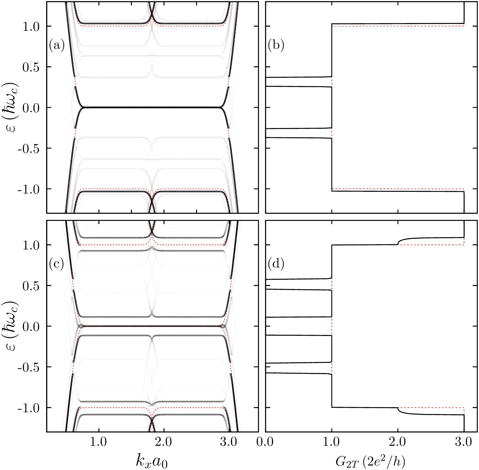
First let us analyze the case of a linearly polarized laser ($\alpha=\pi/2$, $\varphi=0$). The results are shown in Fig. 10 for the off-resonant (top panels) and resonant (bottom panels) situations. For each case, the conductance $G_{2T}$ [(b) and (d)] is shown by the side of the corresponding Landau-Floquet spectral density (projected on the $m=0$ replica) [(a) and (c)]. Here, electron-hole symmetry guarantees that $G_{2T}(-\varepsilon)=G_{2T}(\varepsilon)$.

For an off-resonant photon frequency [$\Omega=0.65\,\omega_{c}$, Figs. 10(a) and 10(b)], two changes appear in the conductance (as compared with that of a non illuminated ribbon shown in red dashed lines): the two dynamical gaps centered at $\pm\,\hbar\Omega/2$, and a small energy shift in the $n=1$ (electron and hole) Landau levels where a transition from $G_{2T}=2e^{2}/h$ to $G_{2T}=6e^{2}/h$ takes place. In the quasienergy region corresponding to the dynamical gaps the conductance is almost completely suppressed in a very sharp way. This is due to the fact that transport is carried out entirely by edge states, which are completely reflected by the laser spot in that particular energy range owed to the appearance of a gap—a related effect was discussed in the case of a driven transition-metal dichalcogenide ribbon in Ref. Huamán and Usaj 2019.

When the photon energy is in resonance with the first non zero Landau level [$\Omega=\omega_{c}$, Figs. 10(c) and 10(d)], the conductance exhibits, in addition to the two dips at $\pm\,\hbar\Omega/2$, a strong suppression coming from the low energy gap created in the Floquet spectrum—it is interesting to note that the faint dispersive states near $\varepsilon=0$ have a negligible contribution to the conductance. Additionally, whereas in a non irradiated sample the conductance jumps from $2e^{2}/h$ to $6e^{2}/h$ when the Fermi energy crosses $\hbar\omega_{c}$ as the result of the change of the number of available edge states with a given chirality from one to three, here an intermediate quasi plateau at $G_{2T}\approx 4e^{2}/h$ appears. As mentioned in the discussion of Fig. 2, this effect is related to the fact that there is a range of quasienergies were the number of effective edge modes is reduced by virtue of the upward energy shift of the Floquet edge mode of one of the valleys (the $K^{\prime}$ valley in the case of Fig. 2). The origin of that shift is the level repulsion between the flat (dispersionless) edge state in the $m=1$ replica and the first dispersive ($\nu_{2}$) edge mode of the $m=0$ replica, which has always a higher quasienergy (this is not the case in the other valley). As such, this happens for opposite valleys in opposite sides of the sample. This explains why in Fig. 10(c) there are no edge modes for $\varepsilon_{\scriptscriptstyle{F}}\sim\hbar\omega_{c}$ near $k_{x}a_{0}\sim 1.8$ for the chosen ribbon’s width. Due to the electron-hole symmetry, a similar argument holds for $\varepsilon_{\scriptscriptstyle{F}}=-\hbar\omega_{c}$.

The results for a circularly polarized laser ($\varphi=2\alpha=\pi/2$) are shown in Fig. 11 for the same photon frequencies. All the prominent features described for the linear case are also observed here, but with the addition of several important new ones:

1. (i)

   In contrast to Figs. 10, here $G_{2T}(-\varepsilon)\neq G_{2T}(\varepsilon)$;

2. (ii)

   When $\Omega=0.65\,\omega_{c}$ the conductance is, apart from the two square dips around $\pm\,\hbar\Omega/2$, quite similar to that of the static system. Notice that bending of the states near $\varepsilon_{\scriptscriptstyle{F}}=0$ induced by the laser provides the channel that leads to $G_{2T}=2e^{2}/h$ near the Dirac point;

3. (iii)

   When $\Omega=\omega_{c}$, the emergence of the new dispersive edge modes near $\varepsilon_{\scriptscriptstyle{F}}\sim 0$ (on the negative side for our choice of polarization) is fully developed. These edge modes are the ones described in Fig. 2 when discussing the properties of the edge modes of the $K^{\prime}$ valley [and the same as those described above in (ii)]. They lead to a quantized conductance that partially fills the gap near zero energy—the narrow dip in the conductance that is observed in that energy region is due to a high-order anticrossing, which cannot be fully appreciated in the Landau-Floquet spectral density [Fig. 11(c)]. The quasi plateau in Fig. 11(d) slightly above $\varepsilon_{\scriptscriptstyle{F}}=\hbar\omega_{c}$ has the same origin as those seen in Fig. 10(d), and can be explained in an analogous manner. The lack of a similar feature at $\varepsilon_{\scriptscriptstyle{F}}=-\hbar\omega_{c}$ comes from the selection rules Eq. (II.4).

We now consider an armchair ribbon of width $W=120\sqrt{3}\,a_{0}$ and keep the same parameters, $\zeta=0.003$ and $z=0.025$. Figure 12 shows the results for a linearly polarized laser ($\alpha=\varphi=0$, in-plane electric field normal to ribbon’s edges). Let us point out first some general considerations. As always with this type of polarization, the Landau-Floquet spectrum presents electron-hole symmetry and thus $G_{2T}(\varepsilon_{\scriptscriptstyle{F}})=G_{2T}(-\varepsilon_{\scriptscriptstyle{F}})$. Moreover, as the Landau-Floquet bands lack the dynamical gaps at $\pm\,\hbar\Omega/2$ (to first order in $z$), $G_{2T}$ does not show the typical strong suppression around these points—at most some minor very narrow features can be observed, corresponding to higher order photon processes. Additionally, for $\varepsilon_{\scriptscriptstyle{F}}$ slightly below (above) $\hbar\omega_{c}$ ($-\hbar\omega_{c}$), where the static conductance changes from $G_{2T}=2e^{2}/h$ to $G_{2T}=6e^{2}/h$, the conductance is rather oscillating, a behavior reminiscent of the $4e^{2}/h$ feature found in the zigzag case—note that, in the latter case, the features appear exactly at $\varepsilon_{\scriptscriptstyle{F}}=\pm\,\hbar\omega_{c}$.

For a non-resonant photon frequency $\Omega=0.65\,\omega_{c}$, Figs. 12(a) and (b), there are not special features around $\varepsilon_{\scriptscriptstyle{F}}=0$. The linear conductance shows a flat profile as a function of $\varepsilon_{\scriptscriptstyle{F}}$, nearly the same as the static system, in agreement with the small changes induced by the laser field on the spectral density.

The situation changes when the laser photon frequency is in resonance, $\Omega=\omega_{c}$, Figs. 12(c) and (d). On the one side, there is a sharp dip around $\varepsilon_{\scriptscriptstyle{F}}=0$. Its limits are roughly defined by the small avoided crossings, coming from the coupling between the replicas $|\bm{\chi}_{\nu_{1}k}^{c},0\rangle$ and $|\bm{\chi}_{\nu_{2}k}^{v},1\rangle$ ($\varepsilon_{\scriptscriptstyle{F}}>0$), and between $|\bm{\chi}_{\nu_{1}k}^{v},0\rangle$ and $|\bm{\chi}_{\nu_{2}k}^{c},-1\rangle$ ($\varepsilon_{\scriptscriptstyle{F}}<0$)—selection rules Eq. (13) state that the matrix element between these pairs of Floquet states is zero, so these gaps originate from higher order processes, which explains their smallness. This dip is not the product of an evanescent penetration inside the scattering region, since from Fig. 12(c) it is clear that there are conducting states there. However, inside the region defined by the avoided crossings mentioned above, the Landau-Floquet states well inside the scattering region, and in a given edge of the ribbon, have the opposite sign of the velocity as compared with the incoming electrons. Therefore, the only way for these electrons to go through the central illuminated region is to move across the width of the ribbon until reach the opposite edge, where available states with a favorable velocity exist. If the laser’s spatial profile (see Fig. 9), is sufficiently smooth or adiabatic, as it is in our calculations, this motion of charge between edges is hindered by the presence of the small gaps introduced above. In this scenario, the fraction of incoming electrons reaching the opposite edge is negligible, and instead most of them simply backscatter into the Floquet channels $m=1$ or $m=-1$, depending on the character (conduction or valence) of the incident electrons. For electrons with energies just above the avoided crossing, the mismatch is still present, although in this case the incident electrons can reach the other edge and transmit into the other lead. This form of transmission is inherently inefficient, although it can be improved by further smoothing out the turning on-off of the laser (not shown). The renormalized (shifted) value of bulk part of $|\bm{\chi}_{\nu_{2}k}^{c},-1\rangle$ marks the onset of a constant conductance $G_{2T}=2e^{2}/h$. Above this value there are two available Landau-Floquet channels, although with only one incident channel the transmittance reduces to $T(\varepsilon_{\scriptscriptstyle{F}})=1$. Due to electron-hole symmetry, this analysis can be extended to negative energies.

On the other hand, near $\varepsilon_{\scriptscriptstyle{F}}=\hbar\omega_{c}$ (similar at $\varepsilon_{\scriptscriptstyle{F}}=-\hbar\omega_{c}$), instead of the well defined change from $T(\varepsilon_{\scriptscriptstyle{F}})=1$ to $T(\varepsilon_{\scriptscriptstyle{F}})=3$ in the non driven system, there is a progressive increase from $1$ to $3$, something that resembles the zigzag case (where an intermediate step with $T(\varepsilon_{\scriptscriptstyle{F}})\simeq 2$ was found).

The circularly polarized case (Fig. 13, $\varphi=2\alpha=\pi/2$) presents similar features, with the expected lack of electron-hole symmetry. It is worth mentioning that the mismatch problem that leads to the suppression of the conductance for $\varepsilon_{\scriptscriptstyle{F}}\simeq 0$ are already apparent in the non resonant case [Figs. 13(a) and (b)], as well as higher order narrow features. What is more, in resonance [Figs. 13(c) and (d), $\Omega=\omega_{c}$] the low energy conductance gap contains some fine structure inside it, which can be understood using the same arguments we introduced when dealing with the linearly polarized case. However, a better and more appealing way to analyse this is to look at the scattering states in Floquet space, as we do in the next section.

In the previous sections we described some of the features of the two-terminal dc conductance in terms of the appearance of gaps in the projected Landau-Floquet spectral density, the emergence of light induced edge states with different chirality, or the mismatch between the leads’ and the system’s wavefunction. All these effects can be made clearer by looking at the Floquet scattering states. Namely, we calculate the (squared) amplitude of the scattered wavefunction corresponding to an incident wave coming from the right lead, for instance, with a given energy in the $m=0$ Floquet replica. The results are shown in Figs. 14 and 15 for the zigzag and the armchair edge terminations, respectively. We have selected four particular values of the incident waves for illustration purposes.

In Fig. 14 (zigzag ribbon, $W=130\,a$) the four selected scattered waves correspond to an incoming wave function with energy: (i) $\varepsilon/\hbar\omega_{c}=1.15$, in which case there are three propagating edge modes in the leads and hence the corresponding equilibrium conductance is $6e^{2}/h$. Of those edge modes, only two can propagate through the irradiated region, as it can be clearly observed in the projected Floquet spectral density shown in Fig. 14(i), while the other is fully reflected at the interface between the two regions (mostly in the $m=0$ replica on the other side of the sample). This leads to the quasi plateau of $4e^{2}/h$ shown in Fig. 11(d); (ii) $\varepsilon=\hbar\Omega/2$, well inside the dynamical gap. Here the incident wave penetrates the scattering region as an evanescent wave before being reflected, on the same side of the sample, into the $m=1$ replica. Hence the conductance is strongly suppressed; (iii) $\varepsilon/\hbar\omega_{c}=0.05$, inside the low energy Floquet gap but above the Dirac point. The incident wave is fully reflected on the $m=-1$ replica but on the other side of the sample; (iv) $\varepsilon/\hbar\omega_{c}=-0.05$. Here the incoming wave, now on the bottom edge of the sample due to its valence band character, is mostly fully transmitted through the $m=0$ channel (with some participation of the $m=-1$ replica). However, quite remarkably, this requires the edge mode to switch edges inside the irradiated region. That is, the Floquet edge mode inside the sample presents the opposite chirality as compared to the one it has on the (non irradiated) leads. As we show in the next section, this leads to a change in the sign of the Hall conductance.

Figure 15 shows the scattering states for an armchair ribbon of width $W=120\,a$. Here we concentrate on a small quasienergy region, $\varepsilon\in[-0.3\,\hbar\omega_{c},0.4\,\hbar\omega_{c}]$, where important departures from the static conductance appear [see Fig. 13(c) and (d)]. For all the quasienergies selected, the static system presents a conductance $G_{2T}$ equal to $2e^{2}/h$, with only one propagating channel coming from the right lead. In every case, we see that most of the incident flux is scattered through the channel $m=-1$, with a negligible component going into the channel $m=1$ (not shown here). This asymmetry in the roles of the Floquet replicas is a consequence of the time-reversal symmetry breaking imposed by the circularly polarized light and the selection rules Eq. (II.4) and (13). Mainly due to the non monotonous bands of the second branch (see Appendix), this case shows some special peculiarities not present in zigzag ribbons.

As before, we consider four relevant cases with different energies: (i) $\varepsilon/\hbar\omega_{c}=0.33$, there are two available channels inside the irradiated region, as the result of the superposition and coupling of two replicas $m=0$ and $m=-1$, for only one incident conduction channel. This leads to the appearance of oscillations in the probability density on each channel and to a displacement of the center of the orbits inside the illuminated region. The period of these oscillations is roughly equal to $2\pi/\delta k$, where $\delta k$ is the difference between the wave vectors $k_{y}$, corresponding to the incident energy $\varepsilon$, of the two Floquet channels inside the sample. The transmittance in this region is almost perfect so $G_{2T}\simeq 2e^{2}/h$; (ii) $\varepsilon/\hbar\omega_{c}=0.022$, the sign of the velocity of the incoming channel matches that of the (only) Floquet states in the irradiated region, and thus transport is possible, although imperfect due to the different spatial profile of both of them (incoming states are more centered towards the bulk while the Landau-Floquet states are closer the edge). This results in a not very well developed peak of conductance [$T(\varepsilon_{\scriptscriptstyle{F}})\sim 0.9$], as it is shown in Fig. 13(d). In (iii) and (iv) the incoming channels move in the opposite direction to those available Landau-Floquet states inside the scattering region and on the same edge. Then, the only way for them to reach the other lead is to scatter into the other edge, where states with the same velocity are available for transport. Because of the adiabatic matching between the wavefunctions (as a consequence of the smooth turning on of the laser field), as it was already discussed in Sec. IV.2, there is a certain energy threshold for this to happen set by the presence of a the small gap between (iii) and (iv) as shown in the Floquet spectral density (see Fig. 15). Then we have the following: (iii) $\varepsilon/\hbar\omega_{c}=-0.044$, here the incoming state cannot go through the avoided crossing and it is mostly reflected backward in the Floquet channel $m=-1$; (iv) $\varepsilon/\hbar\omega_{c}=-0.11$, the the electrons arriving from the right lead can partially go through the avoided crossing in the Floquet spectrum, reaching the other edge of the ribbon. Characteristic of this regimen is the noisy behavior of the conductance as a function of the Fermi level, leading to an incomplete transmission. Below $\varepsilon=-0.07\,\hbar\omega_{c}$, the velocities match and the transmission is perfect ($G_{2T}=2e^{2}/h$).

References

- von Klitzing et al. (1980) K. von Klitzing, G. Dorda, and M. Pepper, “New Method for High-Accuracy Determination of the Fine-Structure Constant Based on Quantized Hall Resistance,” Phys. Rev. Lett. 45, 494 (1980).
- von Klitzing et al. (2020) K. von Klitzing, T. Chakraborty, P. Kim, V. Madhavan, X. Dai, J. McIver, Y. Tokura, L. Savary, D. Smirnova, A. M. Rey, C. Felser, J. Gooth, and X. Qi, “40 years of the quantum Hall effect,” Nature Reviews Physics , 1 (2020).
- Laughlin (1981) R. B. Laughlin, “Quantized Hall conductivity in two dimensions,” Physical Review B 23, 5632 (1981).
- Thouless et al. (1982) D. J. Thouless, M. Kohmoto, M. P. Nightingale, and M. den Nijs, “Quantized Hall Conductance in a Two-Dimensional Periodic Potential,” Phys. Rev. Lett. 49, 405 (1982).
- Hasan and Kane (2010) M. Z. Hasan and C. L. Kane, “Colloquium : Topological insulators,” Rev. Mod. Phys. 82, 3045 (2010).
- Ando (2013) Y. Ando, “Topological Insulator Materials,” Journal of the Physical Society of Japan 82, 102001 (2013).
- Haldane (2017) F. D. M. Haldane, “Nobel Lecture: Topological quantum matter,” Reviews of Modern Physics 89, 040502 (2017).
- König et al. (2007) M. König, S. Wiedmann, C. Brüne, A. Roth, H. Buhmann, L. W. Molenkamp, X.-L. Qi, and S.-C. Zhang, “Quantum Spin Hall Insulator State in HgTe Quantum Wells,” Science 318, 766 (2007).
- Hsieh et al. (2008) D. Hsieh, D. Qian, L. Wray, Y. Xia, Y. S. Hor, R. J. Cava, and M. Z. Hasan, “A topological Dirac insulator in a quantum spin Hall phase,” Nature 452, 970 (2008).
- Xu et al. (2015) S.-Y. Xu, I. Belopolski, N. Alidoust, M. Neupane, G. Bian, C. Zhang, R. Sankar, G. Chang, Z. Yuan, C.-C. Lee, S.-M. Huang, H. Zheng, J. Ma, D. S. Sanchez, B. Wang, A. Bansil, F. Chou, P. P. Shibayev, H. Lin, S. Jia, and M. Z. Hasan, “Discovery of a Weyl Fermion semimetal and topological Fermi arcs,” Science , aaa9297 (2015).
- von Klitzing (2019) K. von Klitzing, “Essay: Quantum Hall Effect and the New International System of Units,” Physical Review Letters 122, 200001 (2019).
- Oka and Aoki (2009a) T. Oka and H. Aoki, “Photovoltaic Hall effect in graphene,” Phys. Rev. B 79, 081406 (2009a).
- Lindner et al. (2011) N. H. Lindner, G. Refael, and V. Galitski, “Floquet topological insulator in semiconductor quantum wells,” Nat Phys 7, 490 (2011).
- Kitagawa et al. (2011) T. Kitagawa, T. Oka, A. Brataas, L. Fu, and E. Demler, “Transport properties of nonequilibrium systems under the application of light: Photoinduced quantum Hall insulators without Landau levels,” Phys. Rev. B 84, 235108 (2011).
- Rudner et al. (2013) M. S. Rudner, N. H. Lindner, E. Berg, and M. Levin, “Anomalous edge states and the bulk-edge correspondence for periodically-driven two dimensional systems,” Phys. Rev. X 3, 031005 (2013).
- Usaj et al. (2014) G. Usaj, P. M. Perez-Piskunow, L. E. F. Foa Torres, and C. A. Balseiro, “Irradiated graphene as a tunable Floquet topological insulator,” Phys. Rev. B 90, 115423 (2014).
- Rudner and Lindner (2020) M. S. Rudner and N. H. Lindner, “Band structure engineering and non-equilibrium dynamics in floquet topological insulators,” Nature Reviews Physics 2, 229 (2020).
- noa (2020) “Quantum phases on demand,” Nature Physics 16, 1 (2020).
- Giustino et al. (2020) F. Giustino, M. Bibes, J. H. Lee, F. Trier, R. Valentí, S. M. Winter, Y.-W. Son, L. Taillefer, C. Heil, A. I. Figueroa, B. Plaçais, Q. Wu, O. V. Yazyev, E. P. A. M. Bakkers, J. Nygård, P. Forn-Díaz, S. de Franceschi, L. E. F. Foa Torres, J. McIver, A. Kumar, T. Low, R. Galceran, S. O. Valenzuela, M. V. Costache, A. Manchon, E.-A. Kim, G. R. Schleder, A. Fazzio, and S. Roche, “The 2020 Quantum Materials Roadmap,” Journal of Physics: Materials (2020), 10.1088/2515-7639/abb74e.
- Wang et al. (2013) Y. H. Wang, H. Steinberg, P. Jarillo-Herrero, and N. Gedik, “Observation of Floquet-Bloch States on the Surface of a Topological Insulator,” Science 342, 453 (2013).
- Mahmood et al. (2016) F. Mahmood, C.-K. Chan, Z. Alpichshev, D. Gardner, Y. Lee, P. A. Lee, and N. Gedik, “Selective scattering between Floquet-Bloch and Volkov states in a topological insulator,” Nature Physics 12, 306 (2016).
- McIver et al. (2020) J. W. McIver, B. Schulte, F.-U. Stein, T. Matsuyama, G. Jotzu, G. Meier, and A. Cavalleri, “Light-induced anomalous Hall effect in graphene,” Nature Physics 16, 38 (2020).
- Wintersperger et al. (2020) K. Wintersperger, C. Braun, F. N. Ünal, A. Eckardt, M. D. Liberto, N. Goldman, I. Bloch, and M. Aidelsburger, “Realization of an anomalous Floquet topological system with ultracold atoms,” Nature Physics , 1 (2020).
- Eckardt (2017) A. Eckardt, “Colloquium: Atomic quantum gases in periodically driven optical lattices,” Reviews of Modern Physics 89, 011004 (2017).
- Cooper et al. (2019) N. Cooper, J. Dalibard, and I. Spielman, “Topological bands for ultracold atoms,” Reviews of Modern Physics 91, 015005 (2019).
- Calvo et al. (2011) H. L. Calvo, H. M. Pastawski, S. Roche, and L. E. F. Foa Torres, “Tuning laser-induced band gaps in graphene,” Appl. Phys. Lett. 98, 232103 (2011).
- Perez-Piskunow et al. (2014) P. M. Perez-Piskunow, G. Usaj, C. A. Balseiro, and L. E. F. Foa Torres, “Floquet chiral edge states in graphene,” Phys. Rev. B 89, 121401(R) (2014).
- Kooi et al. (2018) S. H. Kooi, A. Quelle, W. Beugeling, and C. Morais Smith, “Genesis of the Floquet Hofstadter butterfly,” Physical Review B 98, 115124 (2018).
- Du et al. (2018) L. Du, Q. Chen, A. D. Barr, A. R. Barr, and G. A. Fiete, “Floquet Hofstadter butterfly on the kagome and triangular lattices,” Physical Review B 98, 245145 (2018).
- Wackerl et al. (2019) M. Wackerl, P. Wenk, and J. Schliemann, “Driven Hofstadter butterflies and related topological invariants,” Physical Review B 100, 165411 (2019).
- Zhao et al. (2020) M. Zhao, Q. Chen, X.-D. Tian, and L. Du, “Floquet engineering the Hofstadter butterfly in the square lattice and its effective Hamiltonian,” arXiv:2007.01071 [cond-mat] (2020), arXiv: 2007.01071.
- López et al. (2015) A. López, A. Di Teodoro, J. Schliemann, B. Berche, and B. Santos, “Laser-induced modulation of the Landau level structure in single-layer graphene,” Physical Review B 92, 235411 (2015).
- Ding et al. (2018) K.-H. Ding, L.-K. Lim, G. Su, and Z.-Y. Weng, “Quantum Hall effect in ac driven graphene: From the half-integer to the integer case,” Physical Review B 97, 035123 (2018).
- Dehghani et al. (2015) H. Dehghani, T. Oka, and A. Mitra, “Out-of-equilibrium electrons and the Hall conductance of a Floquet topological insulator,” Physical Review B 91, 155422 (2015).
- Dehghani et al. (2014) H. Dehghani, T. Oka, and A. Mitra, “Dissipative Floquet topological systems,” Physical Review B 90, 195429 (2014).
- Seetharam et al. (2015) K. I. Seetharam, C.-E. Bardyn, N. H. Lindner, M. S. Rudner, and G. Refael, “Controlled Population of Floquet-Bloch States via Coupling to Bose and Fermi Baths,” Physical Review X 5, 041050 (2015).
- Iadecola et al. (2015) T. Iadecola, T. Neupert, and C. Chamon, “Occupation of topological Floquet bands in open systems,” Physical Review B 91, 235133 (2015).
- Dehghani and Mitra (2016) H. Dehghani and A. Mitra, “Occupation probabilities and current densities of bulk and edge states of a Floquet topological insulator,” Physical Review B 93, 205437 (2016).
- Peralta Gavensky et al. (2018) L. Peralta Gavensky, G. Usaj, and C. A. Balseiro, “Time-resolved Hall conductivity of pulse-driven topological quantum systems,” Physical Review B 98, 165414 (2018).
- Schüler et al. (2020) M. Schüler, U. De Giovannini, H. Hübener, A. Rubio, M. A. Sentef, T. P. Devereaux, and P. Werner, “How Circular Dichroism in Time- and Angle-Resolved Photoemission Can Be Used to Spectroscopically Detect Transient Topological States in Graphene,” Physical Review X 10, 041013 (2020).
- Foa Torres et al. (2014) L. E. F. Foa Torres, P. M. Perez-Piskunow, C. A. Balseiro, and G. Usaj, “Multiterminal Conductance of a Floquet Topological Insulator,” Phys. Rev. Lett. 113, 266801 (2014).
- Moskalets and Büttiker (2002) M. Moskalets and M. Büttiker, “Floquet scattering theory of quantum pumps,” Physical Review B 66, 205320 (2002).
- Camalet et al. (2003) S. Camalet, J. Lehmann, S. Kohler, and P. Hänggi, “Current Noise in ac-Driven Nanoscale Conductors,” Phys. Rev. Lett. 90, 210602 (2003).
- (44) This Floquet scattering picture has been demonstrated to be equivalent to the non-equilibium Green’s function formalism in the appropriate limit Kohler et al. 2005 and a dictionary between the two has been pointed out in Ref. Arrachea and Moskalets 2006.
- Castro Neto et al. (2009) A. H. Castro Neto, F. Guinea, N. M. R. Peres, K. S. Novoselov, and A. K. Geim, “The electronic properties of graphene,” Rev. Mod. Phys. 81, 109 (2009).
- Bena and Montambaux (2009) C. Bena and G. Montambaux, “Remarks on the tight-binding model of graphene,” New Journal of Physics 11, 095003 (2009).
- Grifoni and Hänggi (1998) M. Grifoni and P. Hänggi, “Driven quantum tunneling,” Physics Reports 304, 229 (1998).
- Platero and Aguado (2004) G. Platero and R. Aguado, “Photon-assisted transport in semiconductor nanostructures,” Physics Reports 395, 1 (2004).
- Kohler et al. (2005) S. Kohler, J. Lehmann, and P. Hänggi, “Driven quantum transport on the nanoscale,” Physics Reports 406, 379 (2005).
- Shirley (1965) J. H. Shirley, “Solution of the Schrödinger Equation with a Hamiltonian Periodic in Time,” Phys. Rev. 138, B979 (1965).
- Oka and Aoki (2009b) T. Oka and H. Aoki, “Photovoltaic hall effect in graphene,” Phys. Rev. B 79, 081406 (2009b).
- Arrachea and Moskalets (2006) L. Arrachea and M. Moskalets, “Relation between scattering-matrix and Keldysh formalisms for quantum transport driven by time-periodic fields,” Phys. Rev. B 74, 245322 (2006).
- (53) U. Bajpai, M. J. H. Ku, and B. K. Nikolić, “Robustness of quantized transport through edge states of finite length: Imaging current density in floquet topological versus quantum spin and anomalous hall insulators,” 2, 033438.
- Huamán and Usaj (2019) A. Huamán and G. Usaj, “Floquet spectrum and two-terminal conductance of a transition-metal dichalcogenide ribbon under a circularly polarized laser field,” Phys. Rev. B 99, 075423 (2019).
- Groth et al. (2014) C. W. Groth, M. Wimmer, A. R. Akhmerov, and X. Waintal, “Kwant: a software package for quantum transport,” New Journal of Physics 16, 063065 (2014).
- (56) M. Berdakin, E. A. Rodríguez-Mena, and L. E. F. Foa Torres, “Spin-polarized tunable photocurrents,” 2010.11883 .
- Gusynin et al. (2008) V. P. Gusynin, V. A. Miransky, S. G. Sharapov, and I. A. Shovkovy, “Edge states in quantum hall effect in graphene (review article),” Low Temperature Physics 34, 778 (2008).
- Nakada et al. (1996) K. Nakada, M. Fujita, G. Dresselhaus, and M. Dresselhaus, “Edge state in graphene ribbons: Nanometer size effect and edge shape dependence,” Phys. Rev. B 54, 17954 (1996).
- Brey and Fertig (2006a) L. Brey and H. Fertig, “Electronic states of graphene nanoribbons studied with the dirac equation,” Phys. Rev. B 73, 235411 (2006a).
- Brey and Fertig (2006b) L. Brey and H. A. Fertig, “Edge states and the quantized hall effect in graphene,” Phys. Rev. B 73 (2006b), 10.1103/physrevb.73.195408.