A Single Iterative Step for Anytime Causal Discovery

A causal DAG, $\mathcal{D}$, over nodes $\mathbf{V}=\mathbf{O}\cup\mathbf{S}\cup\mathbf{L}$ is denoted by $\mathcal{D}(\mathbf{O},\mathbf{S},\mathbf{L})$, where $\mathbf{O}$, $\mathbf{S}$, and $\mathbf{L}$ represent disjoint sets of observed, selection, and latent variables, respectively. We use a ancestral graph [Richardson and Spirtes 2002] to model the conditional independence relations among the observed variables $\mathbf{O}$ in the causal DAG $\mathcal{D}$. This class of graphical models is useful since for every causal DAG there exits a unique maximal ancestral graph (MAG). In this setting, our method is aimed at recovering the MAG of the true underlying DAG.

We assume the causal Markov and faithfulness assumption, and for CI testing we use either a perfect oracle (independence is derived directly from d-separation in the true DAG), or a statistical independence test (e.g., partial correlation) using observed, non-experimental data. In this setting, the MAG cannot be fully recovered and only a Markov equivalence class, represented by a partial ancestral graph (PAG), can be recovered. In this graph, an invariant edge-mark is denoted by an empty circle ‘—o’. That is, there exists at least one MAG in the equivalence class that has a tail edge-mark and at least one MAG that has an arrowhead at that edge tip.

That is, the observed d-separation relations in two $\mathbf{O}$-equivalent DAGs, $\mathcal{D}_{i}$ and $\mathcal{D}_{j}$, are identical. Spirtes 2001 defines equivalence considering an $n$-oracle for testing conditional independence. It returns “dependence” if the condition set size is larger than $n$, otherwise d-separation is tested and returned. Thus, $n$-$\mathbf{O}$-equivalence class is defined by using the $n$-oracle instead of d-separation in Definition 1.

In an MAG $\MAG$, node $X$ is in $\DSepop(A,B)$ if and only if $X\neq A$ and there is an undirected path between $A$ and $X$ such that every node on the path, except the endpoints, is a collider and is an ancestor of $A$ or $B$ [Spirtes et al. 2000]. Spirtes et al. 2000 defined a super-set of D-Sep that can be determined from the skeleton of the PC algorithm and its identified v-structures. This super-set, denoted $\PDSepop(A,B)$ (note the capitalization of ‘D’), includes all the nodes connected by a path to $A$, where every node on this path, except the end-points, is a collider or part of a triangle, hiding it orientation. It is important to note that this definition of $\PDSepop$ assumes that all conditional independence relations $X_{i}\mathbin{\mathchoice{\hbox to0.0pt{\hbox{$\displaystyle\perp$}\hss}\kern 3.46875pt{}\kern 3.46875pt\hbox{$\displaystyle\perp$}}{\hbox to0.0pt{\hbox{$\textstyle\perp$}\hss}\kern 3.46875pt{}\kern 3.46875pt\hbox{$\textstyle\perp$}}{\hbox to0.0pt{\hbox{$\scriptstyle\perp$}\hss}\kern 2.48856pt{}\kern 2.48856pt\hbox{$\scriptstyle\perp$}}{\hbox to0.0pt{\hbox{$\scriptscriptstyle\perp$}\hss}\kern 1.78203pt{}\kern 1.78203pt\hbox{$\scriptscriptstyle\perp$}}}X_{j}|\boldsymbol{Z}$, such that $\boldsymbol{Z}\in\parentsop_{\MAG}(\{X_{i},X_{j}\})$ are identified. A definition of a smaller super-set of $\DSepop$, called $\PDSeppathop$, was given by Colombo et al. 2012, where there is a path connecting every node $Z\in\PDSeppathop(A,B)$ to $B$. We take special interest in the path that connects any $Z\in\PDSepop(A,B)$ to $A$ and define it as follows.

We propose a single step that is called iteratively, for recovering the underlying equivalence class, represented by a PAG. Each iteration is parameterized by $r$ ($r\in\{0,\ldots,|\mathbf{O}|-1\}$), and given a PAG returned by the previous iteration with $r-1$, each pair of connected nodes $A$ and $B$ are tested for independence conditioned on a set $\mathbf{Z}\subset\mathbf{O}$, such that

1. 1.

   $|\mathbf{Z}|=r$, and

2. 2.

   the length of the shortest PDS-path from $Z\in\mathbf{Z}$ to either $A$ or $B$ is less than $r$.

By parameter $r$, we bind the condition set size to its distance from the tested nodes. That is, the condition set size is bounded by the shortest PDS-path length connecting its nodes to the tested nodes ($A$ and $B$). Only nodes that are at most $r$ edges away, on a PDS-path, from $A$ or $B$ are considered. Then, identified v-structures are oriented and the iteration concludes by repeatedly applying orientation rules until no more edges can be oriented [Spirtes et al. 2000, Zhang 2008]. The full procedure is given in Algorithm 1

For the first iteration, $r=0$ and condition sets of CI tests are empty. In the second iteration $r=1$ and only nodes that are adjacent to the tested nodes are included in the condition set (PDS-path length limit is one edge). Only in succeeding iterations nodes that are not adjacent to the tested nodes may be included.

It is important to note that the result of PDSep_r ($X$, $Y$, $\mathcal{G}$, r), in Algorithm 1-line 10, is an ordered set of possible separating sets $\{\mathbf{Z}_{i}\}_{i}$, where each $\mathbf{Z}_{i}$ contains exactly $r$ nodes. The order in which these sets are assigned to $\mathbf{Z}^{\prime}$ in Algorithm 1 is crucial for reducing the total number of CI test that are performed. A trivial example for an inefficient order is having a condition set consisting of only parents of $A$ or $B$ last in $\{\mathbf{Z}_{i}\}_{i}$. We propose ordering this set according to the average of the shortest PDS-path lengths connecting each node in $\mathbf{Z}_{i}$. That is, for a $\mathbf{Z}\subset\PDSeppathop(X,Y)$, the following value is calculated,

Then, the possible separating sets, $\mathbf{Z}_{i}$ are ordered according to this value. Nevertheless, note that the correctness of the algorithm is invariant to this order.

Our proof relies on the following Lemmas.

In words: the shortest path connecting a node to $A$ or $B$ consists of a subset of nodes of the minimal separating set (denoted by square brackets).

The proposed algorithm consists of two main mechanisms for improving efficiency. First, It gradually performs CI tests of increasing condition set sizes, similarly to the PC algorithm. This is done by including all subsets of $\PDSepop$ having a specific size. Secondly, after iteration $r$ all edges are removed between nodes that are m-separated in the underlying MAG by a minimal set of size at most $r$. Thus, we can complete orienting the graph (using v-structures and orientation rules). Moreover, the definition of $\PDSepop$ relies on a strong assumption that the only edges that were removed, are between nodes that are m-separated given their parents in the MAG. In our case, edges between nodes that are m-separated given any minimal subset of size $r$ are removed. This allows considering super-sets of $\DSepop$ that are smaller than $\PDSepop$, resulting in fewer CI tests. We expect this to be more dominant for CI tests with large condition sets.

Finally, we note that the computational complexity of the algorithm is $O(n^{2k})$, where $n$ is the number of nodes and $k$ is the maximal in-degree. This is because for every pair of nodes $A$ and $B$, the number of CI tests is bounded by the number of subsets of $\PDSepop(A,B)$ and $\PDSepop(A,B)$. That is, a complexity that is polynomial in the number of nodes $n$ given the maximal in-degree $k$.

The proposed ICD algorithm is proved to recover the PAG that corresponds to the true underlying DAG when using a perfect oracle for the CI tests. A perfect oracle is implemented such that it returns d-separation relations in the true DAG. In this experiment, we measure the number of unique¹¹ 1 We implemented a caching mechanism to ensure that the same CI test is not evaluated and counted more than once. CI tests and their condition set sizes that are required for recovering the true PAG, and compare it to those that are required by the FCI algorithm.

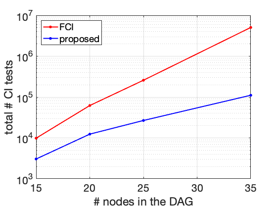
First, we evaluate the total number of CI tests and run-times for different graph sizes. We randomly generate 25 dags for each of the graphs sizes: 15 nodes, 20 nodes, 25 nodes, and 35 nodes. From Figure 1 (a), we find that compared to FCI, the total number of CI tests required by the proposed method increases more slowly with the graph size the the FCI algorithm (note the logarithmic $Y$-axis). From Figure 1 (b) it is evident that the proposed algorithm requires fewer CI tests compared to FCI, for all the 100 tested graphs, and that this advantage of ICD is more evident for graphs that require a larger number of CI tests. From Figure 1 (c) we note that the ratio between the run-times of FCI and ICD increases with the graph size.

Next, we analyze the condition set sizes of the required CI tests. In many CI tests for real-world applications, the statistical power decreases and the computational complexity grows exponentially with the condition set size. In Figure 2 for each tested graph size, we depict the average number of required CI tests per condition set size. It is evident that the saving in number of CI tests, compared to FCI, increases with the graph size.

Lastly, we provide a visualization for the distribution of the ratio between the number of CI tests of FCI and ICD Figure 3. It is evident that the ratio increases with the graph size. Moreover, this distribution is skewed towards larger condition sets and that this skew increases with the graph size.

Finally, we note that in our implementation, the significant reduction in the number of CI tests by ICD compared to FCI, led to a proportional reduction in run-time.

In this experiment, we use the partial-correlation for testing conditional independence (CI) at $\alpha=0.01$, and examine two aspects: accuracy of the learned PAG and the required number of CI tests. For evaluating partial correlation we use data (samples for the observed variables $\mathbf{O}$) in various sizes, $\ell\in[10,1000]$. For each data size, we randomly sample $1000$ DAGs, each having 15 nodes. We learn the PAGs using the proposed ICD algorithm and the FCI algorithm (both are sound and complete).

Required Number of CI Tests. We analyze the total number CI tests required by the proposed algorithm compared to the FCI algorithm. First, using 1000 learned DAGs, we compute the empirical cumulative distribution function $F$ (CDF) for both algorithms on different data sizes. The empirical CDFs for data sizes $100$, $200$, $500$, and $1000$ is depicted in Figure 4. We mark $F(t^{\prime})=0.9$ with dashed horizontal line and with vertical line we mark $t^{\prime}$ in $90\%$. That is, in $90\%$ of the tests (learned DAGs) the algorithm required at most $t^{\prime}$ CI tests. For data sizes $100$, $200$, $500$, and 1000, the ratios between $t^{\prime}$ for our proposed method and FCI are $1.16$, $1.75$, $2.76$, and $3.75$, respectively. It is evident that the ratio increases rapidly for small data sets and starts to converge to some value (the ratio when using perfect CI oracle). We then evaluate statistical significance using the 2-sample Kolmogorov–Smirnov test. The p-values and the statistic are given in Figure 5 (a) and (b), respectively. The value of the Kolmogorov–Smirnov statistic for $\ell\geq 40$ is consistently high compared to its value for smaller data sizes. We conclude that for $\ell\geq 40$ the CDFs of the number of CI tests is different with statistical significance at $\alpha=0.05$. Finally, In Figure 5 (c) we plot the number of CI tests as a function of data set size.

Structural Accuracy. We measure three types of structural errors: (‘extra-edges’) the number of edges present in the learned structure but are not in the true PAG, (‘missing-edges’) the number of edges that are in the true PAG but are missing from the learned PAG, and (’wrong edge-marks’) the number of edge-marks in the learned graph that are different in the true PAG (for edges that exist in both graphs). Compared to the FCI algorithm and for $100\leq\ell\leq 1000$, the proposed method had fewer, (up to $10\%$ for 15 nodes, and $18\%$ for 35 nodes), ‘missing-edges’ and a similar a number of ’extra-edges’ and ’wrong edge-marks’. We report the ratio in total number of structural errors for graphs having 15 nodes, as a function of the data set size in Figure 5 (d).

References

- Pearl [2010] Judea Pearl. An introduction to causal inference. The international journal of biostatistics, 6(2), 2010.
- Spirtes [2010] Peter Spirtes. Introduction to causal inference. Journal of Machine Learning Research, 11(May):1643–1662, 2010.
- Pearl [2009] Judea Pearl. Causality: Models, Reasoning, and Inference. Cambridge university press, second edition, 2009.
- Spirtes et al. [2000] Peter Spirtes, Clark Glymour, and Richard Scheines. Causation, Prediction and Search. MIT Press, 2nd edition, 2000.
- Peters et al. [2017] Jonas Peters, Dominik Janzing, and Bernhard Schölkopf. Elements of causal inference. The MIT Press, 2017.
- Rohekar et al. [2018] Raanan Y Rohekar, Yaniv Gurwicz, Shami Nisimov, Guy Koren, and Gal Novik. Bayesian structure learning by recursive bootstrap. In Advances in Neural Information Processing Systems (NeurIPS), 2018.
- Yehezkel and Lerner [2009] Raanan Yehezkel and Boaz Lerner. Bayesian network structure learning by recursive autonomy identification. Journal of Machine Learning Research (JMLR), 10(Jul):1527–1570, 2009.
- Cooper and Herskovits [1992] Gregory F Cooper and Edward Herskovits. A Bayesian method for the induction of probabilistic networks from data. Machine learning, 9(4):309–347, 1992.
- Chickering [2002] David Maxwell Chickering. Optimal structure identification with greedy search. Journal of machine learning research, 3(Nov):507–554, 2002.
- Shimizu et al. [2006] Shohei Shimizu, Patrik O Hoyer, Aapo Hyvärinen, and Antti Kerminen. A linear non-gaussian acyclic model for causal discovery. Journal of Machine Learning Research, 7(Oct):2003–2030, 2006.
- Hoyer et al. [2009] Patrik O Hoyer, Dominik Janzing, Joris M Mooij, Jonas Peters, and Bernhard Schölkopf. Nonlinear causal discovery with additive noise models. In Advances in neural information processing systems, pages 689–696, 2009.
- Richardson and Spirtes [2002] Thomas Richardson and Peter Spirtes. Ancestral graph markov models. The Annals of Statistics, 30(4):962–1030, 2002.
- Jaber et al. [2018] Amin Jaber, Jiji Zhang, and Elias Bareinboim. Causal identification under markov equivalence. In 34th Conference on Uncertainty in Artificial Intelligence, pages 978–987. Association for Uncertainty in Artificial Intelligence (AUAI), 2018.
- Jaber et al. [2019] Amin Jaber, Jiji Zhang, and Elias Bareinboim. Causal identification under markov equivalence: Completeness results. In International Conference on Machine Learning, pages 2981–2989, 2019.
- Colombo et al. [2012] Diego Colombo, Marloes H Maathuis, Markus Kalisch, and Thomas S Richardson. Learning high-dimensional directed acyclic graphs with latent and selection variables. The Annals of Statistics, pages 294–321, 2012.
- Claassen et al. [2013] Tom Claassen, Joris M Mooij, and Tom Heskes. Learning sparse causal models is not NP-hard. In Uncertainty in Artificial Intelligence, page 172. Citeseer, 2013.
- Ogarrio et al. [2016] Juan Miguel Ogarrio, Peter Spirtes, and Joe Ramsey. A hybrid causal search algorithm for latent variable models. In Conference on Probabilistic Graphical Models, pages 368–379, 2016.
- Spirtes [2001] Peter Spirtes. An anytime algorithm for causal inference. In AISTATS, 2001.
- Zhang [2008] Jiji Zhang. On the completeness of orientation rules for causal discovery in the presence of latent confounders and selection bias. Artificial Intelligence, 172(16-17):1873–1896, 2008.