跳到论文正文
W Papers独立论文阅读器 arXiv:2012.07491 论文正文 计算阅读时间 · 0%
引用这篇论文根据当前论文元数据生成,正式投稿前建议核对。


License: arXiv.org perpetual non-exclusive license
arXiv:2012.07491v2 [math.OC] 25 Sep 2021

Pursuit of the Cluster Structure of Network Lasso:
Recovery Condition and Non-convex Extension

Shotaro Yagishita Note: Department of Industrial and Systems Engineering, Chuo University, Japan (a15.fjng@g.chuo-u.ac.jp, jgoto@indsys.chuo-u.ac.jp).    Jun-ya Gotoh22footnotemark: 2
Abstract

Network Lasso (NL for short) is a methodology for estimating models by simultaneously clustering data samples and fitting the models to the samples. It often succeeds in forming clusters thanks to the geometry of the ℓ1\ell_{1}-regularizer employed therein, but there might be limitations because of the convexity of the regularizer. This paper focuses on the cluster structure that NL yields and reinforces it by developing a non-convex extension, which we call Network Trimmed Lasso (NTL for short). Specifically, we first study a sufficient condition that guarantees the recovery of the latent cluster structure of NL on the basis of the result of Sun et al. (2021) for Convex Clustering, which is a special case of NL for clustering. Second, we extend NL to NTL to incorporate a cardinality (or, ℓ0\ell_{0}-)constraint and rewrite the constrained optimization problem defined with the ℓ0\ell_{0} norm, a discontinuous function, into an equivalent unconstrained continuous optimization problem. We develop ADMM algorithms to solve NTL and provide its convergence results. Numerical illustrations demonstrate that the non-convex extension provides a more clear-cut cluster structure when NL fails to form clusters without incorporating prior knowledge of the associated parameters.

1 Introduction

In data analysis, fundamental methodologies such as regression and clustering can be enhanced by coupling with side information about the underlying structure of the data set. For example, consider a situation where a batch of data samples consists of outcomes from multiple sources and the analyst knows their (possibly, partial) relationship. In such situations, we can estimate multiple models to fit to the dataset while detecting clusters of the samples. To accomplish such tasks, Hallac et al. 2015 recently have proposed Network Lasso (NL for short).

Let ai∈ℝpa_{i}\in\mathbb{R}^{p} and bi∈ℝb_{i}\in\mathbb{R} denote pp inputs and a real-valued output, respectively, of the ii-th sample, i∈[n]:={1,…,n}i\in[n]:=\{1,...,n\}, and assume that the analyst knows that some of them are similar. If such similarity for i,j∈[n]i,j\in[n] is given by non-negative weights, w~{i,j}\tilde{w}_{\{i,j\}}, its NL version of the ordinary least squares regression is cast as the following convex optimization:

minimizex1,…,xn∈ℝp\displaystyle\underset{x_{1},...,x_{n}\in\mathbb{R}^{p}}{\text{minimize}} 12∑i∈[n](bi−ai⊤xi)2+γ∑i,j∈[n]:i<jw~{i,j}∥xi−xj∥2,\displaystyle\quad\frac{1}{2}\sum_{i\in[n]}(b_{i}-a_{i}^{\top}x_{i})^{2}+\gamma\sum_{i,j\in[n]:i<j}\tilde{w}_{\{i,j\}}\|x_{i}-x_{j}\|_{2}, (1)

where ‖z‖2:=∑j=1pzj2\|z\|_{2}:=\sqrt{\sum_{j=1}^{p}z_{j}^{2}} denotes the ℓ2\ell_{2} norm of a vector z∈ℝpz\in\mathbb{R}^{p}, and γ>0\gamma>0 is a parameter to be tuned so as to strike a balance between the first and second terms of (1). Intuitively, reducing the first term prompts a model (b=a⊤​xib=a^{\top}x_{i}) to fit each sample (ai,bi)(a_{i},b_{i}), while reducing the second term expedites the mergers of similar samples since the weight w~{i,j}\tilde{w}_{\{i,j\}} being large means that the samples ii and jj are similar to each other. Especially, the second term is the sum of ℓ2\ell_{2} norms and, for large γ\gamma, an optimal solution (x1⋆,…,xn⋆)(x^{\star}_{1},...,x^{\star}_{n}) is expected to satisfy ‖xi⋆−xj⋆‖2=0\|x^{\star}_{i}-x^{\star}_{j}\|_{2}=0 for many pairs {i,j}∈ℰ\{i,j\}\in\mathcal{E}. This contraction property is parallel to the group Lasso [22].

In general, let us introduce a weighted undirected graph 𝒢=(𝒱,ℰ,W)\mathcal{G}=(\mathcal{V},\mathcal{E},W), where the vertex set 𝒱=[n]\mathcal{V}=[n] denotes the index set of samples, the edge set ℰ⊂{{i,j}:i,j∈[n];i≠j}\mathcal{E}\subset\{\{i,j\}:i,j\in[n];\,i\neq j\} indicates the pairwise adjacency or similarity, and W=(w{i,j}){i,j}∈ℰ∈ℝ≥0|ℰ|W=(w_{\{i,j\}})_{\{i,j\}\in\mathcal{E}}\in\mathbb{R}^{\left|\mathcal{E}\right|}_{\geq 0} denotes non-negative weights on all the edges to represent the pairwise similarity. (The more w{i,j}w_{\{i,j\}}, the closer the vertices ii and jj.) Let fi:ℝp→ℝf_{i}:\mathbb{R}^{p}\rightarrow\mathbb{R} be a loss function for sample i∈[n]i\in[n]. NL [9] is then formulated as the following optimization problem:

minimizex1,…,xn∈ℝp\displaystyle\underset{x_{1},\ldots,x_{n}\in\mathbb{R}^{p}}{\text{minimize}} ∑i∈𝒱fi​(xi)+γ​∑{i,j}∈ℰw{i,j}​‖xi−xj‖2.\displaystyle\quad\sum_{i\in\mathcal{V}}f_{i}(x_{i})+\gamma\sum_{\{i,j\}\in\mathcal{E}}w_{\{i,j\}}\|x_{i}-x_{j}\|_{2}. (2)

Obviously, (1) is an example of NL (2), where the sum of squared residuals, fi​(xi)=12​(bi−ai⊤​xi)2f_{i}(x_{i})=\frac{1}{2}(b_{i}-a_{i}^{\top}x_{i})^{2}, i∈[n]i\in[n], are employed as the loss functions. NL includes other methods as special cases. If only the input vectors ai∈ℝp,i∈[n]a_{i}\in\mathbb{R}^{p},i\in[n], are given and we employ

fi​(xi)=12​‖xi−ai‖22,f_{i}(x_{i})=\frac{1}{2}\|x_{i}-a_{i}\|_{2}^{2}, (3)

and set ℰ={{i,j}:i,j∈[n];i≠j}\mathcal{E}=\{\{i,j\}:i,j\in[n];\,i\neq j\} and w{i,j}=1w_{\{i,j\}}=1, NL (2) is reduced to Convex Clustering (Pelckmans et al. 2005). Lindsten et al. 2011 and Hocking et al. 2011 consider extensions where w{i,j}w_{\{i,j\}} are not necessarily equal to 11. With an optimal solution (x1∗,…,xn∗)(x_{1}^{*},...,x_{n}^{*}), nodes ii and jj are assigned to the same cluster if and only if xi∗=xj∗x_{i}^{*}=x_{j}^{*}. We call xi∗x_{i}^{*} the centroid of node ii. Namely, samples that share the same centroid form a cluster. For sufficiently large γ\gamma, a clustering result of the data set a1,…,ana_{1},...,a_{n} is obtained thanks to the exact contraction property of the second term of (2). Recent works have reported that NL numerically performs well in various tasks when prior information about the similarity between nodes (i.e., WW) are given appropriately (e.g., Hallac et al. 2015, Jung et al. 2018, Hocking et al. 2011, Chi and Lange 2015, Sun et al. 2021).

In this paper, we further investigate and extend NL with a focus on its clustering property. First, we study whether NL can recover true latent clusters. For Convex Clustering, Zhu et al. 2014, Panahi et al. 2017 and Sun et al. 2021 provide sufficient conditions for recovering the set of the latent clusters. For NL (not limited to Convex Clustering), although Jung et al. 2018 and Jung and Tran 2019 analyze the gap between the optimal solution of NL and true parameter values. However, their conditions do not guarantee the recovery of the true clusters. In contrast, we provide sufficient conditions to recover the latent clusters for NL. The easiness of the recovery will be given by ranges of the parameter γ\gamma, for which NL (2) recovers the (unseen) true clusters if they exist.

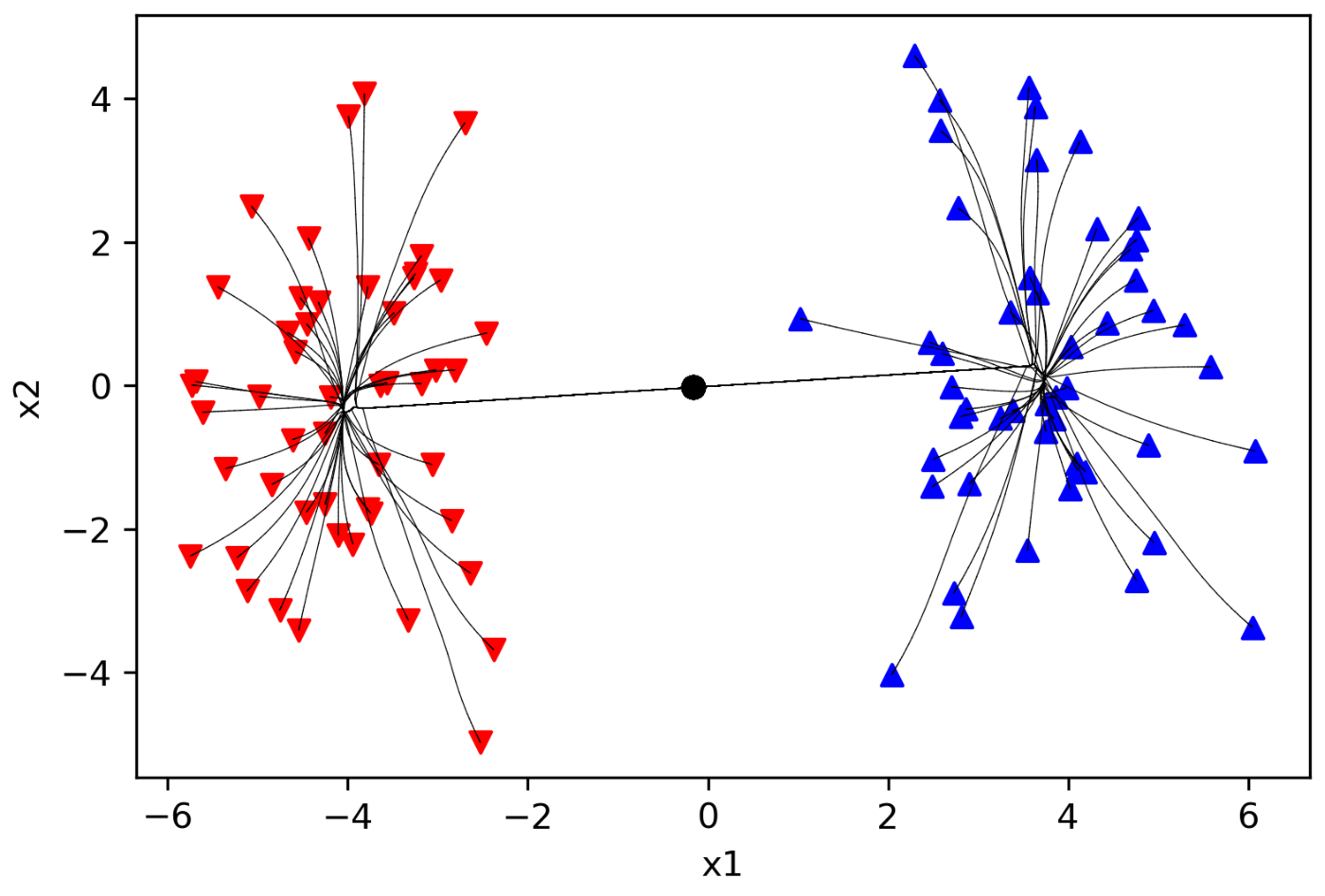
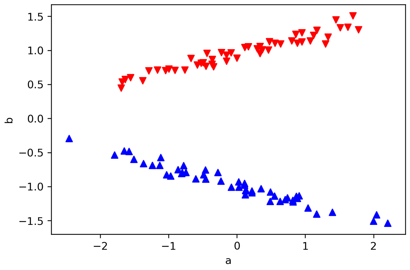
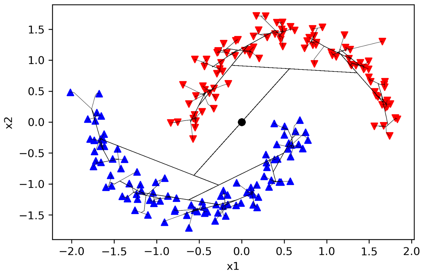
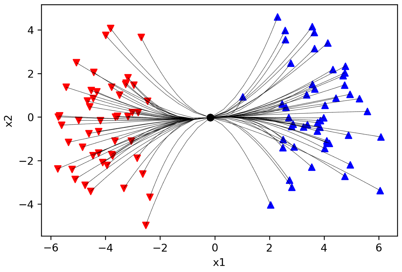
Besides, it is almost certain that there is a gap between Convex Clustering and the usual kk-means approach (or its non-convex optimization version). The second part of this paper is devoted to building a bridge between the two realms: convex vs. non-convex. We should emphasize here that the performance of (2) highly depends on how the analyst puts the prior information of the weights WW. The left panel of Figure 1 shows the regularization paths, i.e., the loci of the centroids obtained by Convex Clustering without prior information (i.e., w(i,j)=1w_{(i,j)}=1 for all (i,j)∈ℰ(i,j)\in\mathcal{E}). While there are two latent clusters (red and blue), all the centroids shrink to the middle point in an equal manner and we cannot obtain the two clusters even with a big γ\gamma. For a practical use of Convex Clustering, it is often suggested to set the weights w{i,j}w_{\{i,j\}}, as w{i,j}=exp⁡(−α​‖ai−aj‖22)w_{\{i,j\}}=\exp(-\alpha\|a_{i}-a_{j}\|_{2}^{2}), where α>0\alpha>0 is a parameter. The right panel of Figure 1 demonstrates that, with this technique, Convex Clustering resulted in a clear-cut clustering. We should note that how to provide such prior information depends on tasks and there are no general tips for NL (2) (e.g., for regression).

To overcome such difficulty, we consider introducing a cardinality constraint in place of the group l2l_{2}-penalty in NL (2). We show that the cardinality-constrained problem can be equivalently rewritten by a non-convex but continuous unconstrained optimization problem, which we call Network Trimmed Lasso (NTL for short). This reformulation is parallel to that for the Trimmed Lasso, which is studied by, for example, Gotoh et al. 2018, Bertsimas et al. 2017, and Amir et al. 2020. We also propose algorithms based on Alternating Direction Method of Multipliers (ADMM) to solve NTL. For a non-convex subproblem in the proposed algorithms, a closed-form solution is derived. Also, we show the convergence of Proximal ADMM, which is an extension of ADMM, to a locally optimal solution of NTL, a non-convex optimization problem. The advantages of NTL over ordinary NL are demonstrated through numerical experiments.
Refer to caption Refer to caption
(a) Without prior information (b) With prior information
Figure 1: Failed cluster path of centroids via Convex Clustering without prior information (left panel (a)) and successful cluster path with prior information, where w{i,j}=e−0.1​‖ai−aj‖22w_{\{i,j\}}=\mathrm{e}^{-0.1{\|a_{i}-a_{j}\|}_{2}^{2}} (right panel (b)).

As the regularization parameter γ\gamma grows, all the centroids are reduced to the mean of nn points, i.e., 1n​∑i∈𝒱ai\frac{1}{n}\sum_{i\in\mathcal{V}}a_{i}, which is located near the origin in each picture. The left-hand side panel shows the result of Convex Clustering with w{i,j}=1w_{\{i,j\}}=1, failing to form clusters even for large γ\gamma’s. On the other hand, the right-hand side panel shows the case where the distance of points is used succeeded in providing a clear-cut cluster structure even with small γ\gamma’s.

Contributions of the paper are summarized as follows:

  • •

    We give a theoretical guarantee that the clustering based on NL works well when prior information is properly provided. Specifically, sufficient conditions with which NL can recover the latent cluster structure are given.

  • •

    We propose a framework of NTL to enhance the cluster structure of NL. More specifically, we show the equivalence between the cardinality-constrained extension of NL and NTL.

  • •

    We present ADMM-based algorithms to solve a problem that has a general Trimmed Lasso penalty, and show that under mild conditions it converges to a local optimum.

The rest of this paper is organized as follows. The next section is devoted to show sufficient conditions that NL recovers a latent cluster structure. Section 3 introduces a cardinality-constrained version of NL to get a more distinguishing cluster structure than NL does. The equivalence between the cardinality-constrained problem and NTL is shown. In Section 4, we develop algorithms for NTL and provide its convergence results. Section 5 reports numerical examples to demonstrate the effectiveness of NTL. Finally, Section 6 concludes the paper.

Notation and preliminaries

A continuous differentiable function f:ℝp→ℝf:\mathbb{R}^{p}\to\mathbb{R} is said to be LL-smooth if there exists L>0L>0 such that

‖∇f​(x)−∇f​(y)‖2≤L​‖x−y‖2\displaystyle\|\nabla f(x)-\nabla f(y)\|_{2}\leq L\|x-y\|_{2} (4)

for any x,y∈ℝx,y\in\mathbb{R}. If ff is LL-smooth, then the inequality

f(y)≤f(x)+∇f(x)⊤(y−x)+L2∥x−y∥22\displaystyle f(y)\leq f(x)+\nabla f(x)^{\top}(y-x)+\frac{L}{2}{\|x-y\|}_{2}^{2} (5)

holds for all x,y∈ℝpx,y\in\mathbb{R}^{p}, which implies L2∥⋅∥22−f\frac{L}{2}\|\cdot\|_{2}^{2}-f is convex (see, e.g., [2, Lemma 5.7]). For a differentiable convex function f:ℝp→ℝf:\mathbb{R}^{p}\to\mathbb{R}, the following statements are equivalent ([2, Theorem 5.8]):

  • •

    ff is LL-smooth.

  • •

    The inequality (5) holds for all x,y∈ℝpx,y\in\mathbb{R}^{p}.

  • •

    L2∥⋅∥22−f\frac{L}{2}\|\cdot\|_{2}^{2}-f is convex.

For a convex function f:ℝp→ℝf:\mathbb{R}^{p}\to\mathbb{R}, the subdifferential of ff at x∈ℝpx\in\mathbb{R}^{p} is defined by

∂f(x):={z∈ℝp∣f(y)≥f(x)+z⊤(y−x)∀y∈ℝp}.\displaystyle\partial f(x):=\{z\in\mathbb{R}^{p}\mid f(y)\geq f(x)+z^{\top}(y-x)\quad\forall y\in\mathbb{R}^{p}\}. (6)

Note that ∂f⁡(x)≠∅\partial f(x)\neq\emptyset ([2, Theorem 3.14]). We call f:ℝp→ℝf:\mathbb{R}^{p}\rightarrow\mathbb{R} strongly convex with a positive constant α\alpha (or simply, α\alpha-strongly convex) if f−α2∥⋅∥22f-\frac{\alpha}{2}\|\cdot\|_{2}^{2} is a convex function. If ff is α\alpha-strongly convex, by using Theorems 3.63 and 5.24 of [2] and the Cauchy-Schwarz inequality, we obtain

‖z‖2≥α​‖x−x¯‖2,\displaystyle\|z\|_{2}\geq\alpha\|x-\overline{x}\|_{2}, (7)

for all x∈ℝp,z∈∂f⁡(x)x\in\mathbb{R}^{p},z\in\partial f(x), where x¯∈argminx∈ℝpf⁡(x)\overline{x}\in\mathop{\rm argmin}\limits_{x\in\mathbb{R}^{p}}f(x) and its existence and uniqueness are guaranteed by strong convexity of ff ([2, Theorem 5.25]). It is also known (e.g., [2, Theorem 5.25]) that if ff is α\alpha-strongly convex and x¯∈argminx∈ℝpf⁡(x)\overline{x}\in\mathop{\rm argmin}\limits_{x\in\mathbb{R}^{p}}f(x), the inequality

α2​‖x−x¯‖22≤f⁡(x)−f⁡(x¯),\displaystyle\frac{\alpha}{2}\|x-\overline{x}\|_{2}^{2}\leq f(x)-f(\overline{x}), (8)

holds for all x∈ℝpx\in\mathbb{R}^{p}. The directional derivative of f:ℝp→ℝf:\mathbb{R}^{p}\to\mathbb{R} at a point x∈ℝpx\in\mathbb{R}^{p} in the direction v∈ℝpv\in\mathbb{R}^{p} is defined by

d​f​(x,v):=limη↘0f⁡(x+η​v)−f⁡(x)η.\displaystyle{\mathrm{d}}f(x;v):=\lim_{\eta\searrow 0}\frac{f(x+\eta v)-f(x)}{\eta}. (9)

A point x∗∈ℝpx^{*}\in\mathbb{R}^{p} is called a (directional-)stationary point of an optimization problem minx⁡f⁡(x)\min\limits_{x}f(x) if the directional derivative d​f​(x∗,v){\mathrm{d}}f(x^{*};v) exists and is non-negative for any v∈ℝpv\in\mathbb{R}^{p}. The maximum and minimum eigenvalues of a symmetric matrix AA are denoted by λmax​(A)\lambda_{\max}(A) and λmin​(A)\lambda_{\min}(A), respectively.

2 Recovery conditions for Network Lasso

In this section, we show the recovery conditions for NL (2) to identify the latent cluster structure on the basis of Sun et al. 2021, which develops sufficient conditions for the recovery of the latent cluster structure for Convex Clustering.

Let C1,…,CNC_{1},...,C_{N} denote (unseen) NN clusters, which satisfy that Ci∩Cj=∅C_{i}\cap C_{j}=\emptyset if i≠ji\neq j, and C1∪⋯∪CN=𝒱C_{1}\cup\cdots\cup C_{N}=\mathcal{V}. We assume that each sample i∈𝒱i\in\mathcal{V} belongs to one of C1,…,CNC_{1},...,C_{N}.

To define the recovery of the cluster structure, we introduce a couple of notions, as below, following [20].

Definition 1.

Let 𝒫:={C1,…,CN}\mathcal{P}:=\{{C}_{1},\ldots,{C}_{N}\} and 𝒫¯:={C¯1,…,C¯M}\overline{\mathcal{P}}:=\{\overline{C}_{1},\ldots,\overline{C}_{M}\} be partitionings of 𝒱\mathcal{V}.

  1. 1.

    When 𝒫¯=𝒫\overline{\mathcal{P}}=\mathcal{P}, we say that 𝒫¯\overline{\mathcal{P}} perfectly recovers 𝒫\mathcal{P}.

  2. 2.

    We call 𝒫¯\overline{\mathcal{P}} a coarsening of 𝒫\mathcal{P} if for any C¯∈𝒫¯\overline{C}\in\overline{\mathcal{P}} there exists I⊂{1,…,N}I\subset\{1,\ldots,N\} such that C¯=∪l∈ICl\overline{C}=\cup_{l\in I}{C}_{l}. Moreover, 𝒫¯\overline{\mathcal{P}} is called the trivial coarsening if 𝒫¯={𝒱}\overline{\mathcal{P}}=\{\mathcal{V}\}. Otherwise, it is called a non-trivial coarsening.

A partitioning represents a cluster structure of the data set 𝒱\mathcal{V}. In the remainder of this paper, we use 𝒫\mathcal{P} to refer to the partitioning corresponding to the true (usually, unseen) cluster structure. For the partitioning 𝒫={C1,…,CN}\mathcal{P}=\{{C}_{1},\ldots,{C}_{N}\}, we introduce the following notation:

nk\displaystyle n_{k} :=|Ck|,\displaystyle:=|C_{k}|, k∈[N],\displaystyle k\in[N], (size of Cluster ​k​)\displaystyle\quad\small\text{(size of Cluster }k\text{)}
wi(k)\displaystyle w_{i}^{(k)} :=∑j∈Ckw{i,j},\displaystyle:=\sum_{j\in C_{k}}w_{\{i,j\}}, i∈𝒱,k∈[N],\displaystyle i\in\mathcal{V},k\in[N], (sum of weights of Sample ​i​ adjacent to Cluster ​k​)\displaystyle\quad\small\text{(sum of weights of Sample }i\text{ adjacent to Cluster }k\text{)}
w(k,k′)\displaystyle w^{(k,k^{\prime})} :=∑i∈Ck∑j∈Ck′w{i,j},\displaystyle:=\sum_{i\in C_{k}}\sum_{j\in C_{k^{\prime}}}w_{\{i,j\}}, k,k′∈[N].\displaystyle k,k^{\prime}\in[N]. (sum of weights between Clusters ​k​ and ​k′​)\displaystyle\quad\small\text{(sum of weights between Clusters }k\text{ and }k^{\prime}\text{)}

For the sake of simplicity, we set w{i,j}=0w_{\{i,j\}}=0 for {i,j}∉ℰ\{i,j\}\notin\mathcal{E} in this section.

Theorem 1.

Suppose that fif_{i} is strictly convex and LiL_{i}-smooth, i∈𝒱i\in\mathcal{V}. Let 𝒫={C1,…,CN}\mathcal{P}=\{{C}_{1},\ldots,{C}_{N}\} be the (unseen) true partitioning of 𝒱\mathcal{V}, and let f(k):=∑i∈Ckfi,k∈[N]f^{(k)}:=\sum_{i\in{C}_{k}}f_{i},~k\in[N]. Assume that for each k∈[N]k\in[N], f(k)f^{(k)} is αk\alpha_{k}-strongly convex, and let x¯(k)=argminx∈ℝpf(k)​(x){\overline{x}}^{(k)}=\mathop{\rm argmin}\limits_{x\in\mathbb{R}^{p}}f^{(k)}(x). Suppose that x¯(k)≠x¯(k′){\overline{x}}^{(k)}\neq{\overline{x}}^{(k^{\prime})} for k≠k′k\neq k^{\prime}. Let

μi​j(k)\displaystyle\mu_{ij}^{(k)} =∑l≠k|wi(l)−wj(l)|+Li+Ljαk​∑l≠kw(k,l),\displaystyle=\sum_{l\neq k}\left|w_{i}^{(l)}-w_{j}^{(l)}\right|+\frac{L_{i}+L_{j}}{\alpha_{k}}\sum_{l\neq k}w^{(k,l)}, i,j∈Ck,k∈[N],\displaystyle i,j\in C_{k},k\in[N],

and suppose that nk​w{i,j}>μi​j(k)n_{k}w_{\{i,j\}}>\mu_{ij}^{(k)} for all i,j∈Ck,k∈[N]i,j\in C_{k},k\in[N] s.t. i≠ji\neq j. Let

γmax\displaystyle\gamma_{\max} :=mink≠k′⁡{‖x¯(k)−x¯(k′)‖21αk​∑l≠kw(k,l)+1αk′​∑l≠k′w(k′,l)},\displaystyle:=\min_{k\neq k^{\prime}}\left\{\frac{{\|{\overline{x}}^{(k)}-{\overline{x}}^{(k^{\prime})}\|}_{2}}{\frac{1}{\alpha_{k}}\sum\limits_{l\neq k}w^{(k,l)}+\frac{1}{\alpha_{k^{\prime}}}\sum\limits_{l\neq k^{\prime}}w^{(k^{\prime},l)}}\right\},
γmin\displaystyle\gamma_{\min} :=maxk⁡maxi,j∈Cki≠j​{‖∇fj​(x¯(k))−∇fi​(x¯(k))‖2nk​w{i,j}−μi​j(k)},\displaystyle:=\max_{k}\max_{\begin{subarray}{c}i,j\in{C}_{k}\\ i\neq j\end{subarray}}\left\{\frac{{\left\|\nabla f_{j}({\overline{x}}^{(k)})-\nabla f_{i}({\overline{x}}^{(k)})\right\|}_{2}}{n_{k}w_{\{i,j\}}-\mu_{ij}^{(k)}}\right\},

where we set a0=∞\frac{a}{0}=\infty for a>0a>0.

Let (x1∗,…,xn∗)(x_{1}^{*},...,x_{n}^{*}) be an optimal solution to (2), and 𝒫¯\overline{\mathcal{P}} be the quotient set of 𝒱\mathcal{V} by equivalence relation xi∗=xj∗{x}_{i}^{*}={x}_{j}^{*}.

  1. 1.

    If γmin≤γ<γmax\gamma_{\min}\leq\gamma<\gamma_{\max}, 𝒫¯\overline{\mathcal{P}} perfectly recovers 𝒫\mathcal{P}.

  2. 2.

    If γmin≤γ<maxk⁡‖∇f(k)​(x¯)‖2∑l≠kw(k,l)\gamma_{\min}\leq\gamma<\max_{k}\frac{{\|\nabla f^{(k)}(\overline{x})\|}_{2}}{\sum\limits_{l\neq k}w^{(k,l)}}, 𝒫¯\overline{\mathcal{P}} is a non-trivial coarsening of 𝒫\mathcal{P}, where

    x¯:=argminx∈ℝp∑k∈[N]f(k)​(x)=argminx∈ℝp∑i∈𝒱fi​(x).\displaystyle\overline{x}:=\mathop{\rm argmin}\limits_{x\in\mathbb{R}^{p}}\sum\limits_{k\in[N]}f^{(k)}(x)=\mathop{\rm argmin}\limits_{x\in\mathbb{R}^{p}}\sum\limits_{i\in\mathcal{V}}f_{i}(x).

Before proving the theorem, let us notice a couple of remarks on its statement.

Remark 1.

Theorem 1 implies that if the weights (w{i,j}){i,j}∈ℰ(w_{\{i,j\}})_{\{i,j\}\in\mathcal{E}} are chosen adequately, NL is guaranteed to return the true cluster structure {C1,…,CN}\{C_{1},...,C_{N}\} at some point on the cluster path. To see this through an example, let us suppose that 𝒢\mathcal{G} is a complete graph ℰ={{i,j}∣i≠j,i,j∈𝒱}\mathcal{E}=\{\{i,j\}\mid i\neq j,~i,j\in\mathcal{V}\}, {fi}i∈𝒱\{f_{i}\}_{i\in\mathcal{V}} satisfies the assumption of Theorem 1, and consider the weights defined as

w{i,j}​{≤w,(i∈Ck,j∈Ck′,k≠k′),=1,(i,j∈Ck,i≠j),\displaystyle w_{\{i,j\}}\left\{\begin{array}[]{ll}\leq w,&(i\in{C}_{k},\ j\in{C}_{k^{\prime}},\ k\neq k^{\prime}),\\ =1,&(i,j\in{C}_{k},\ i\neq j),\end{array}\right.

for a constant w∈[0,1]w\in[0,1]. Note that when ww is equal to 11, we can say the weights have no information; as ww gets closer to 00, the weights more reflect the true cluster structure. Observing that

∑l≠kw(k,l)≤∑l≠knk​nl​w≤n2​w→0(w→0)\displaystyle\sum\limits_{l\neq k}w^{(k,l)}\leq\sum\limits_{l\neq k}n_{k}n_{l}w\leq n^{2}w\rightarrow 0\quad(w\rightarrow 0) (12)

for all k∈[N]k\in[N] and

∑l≠k|wi(l)−wj(l)|≤∑l≠knl​w≤n​w→0(w→0)\displaystyle\sum_{l\neq k}\left|w_{i}^{(l)}-w_{j}^{(l)}\right|\leq\sum_{l\neq k}n_{l}w\leq nw\rightarrow 0\quad(w\rightarrow 0) (13)

for all i,j∈Ck,k∈[N]i,j\in C_{k},k\in[N], we have

γmax\displaystyle\gamma_{\max} →∞,\displaystyle\rightarrow\infty, (14)
γmin\displaystyle\gamma_{\min} →maxk⁡maxi,j∈Cki≠j​{‖∇fj​(x¯(k))−∇fi​(x¯(k))‖2nk},\displaystyle\rightarrow\max_{k}\max_{\begin{subarray}{c}i,j\in{C}_{k}\\ i\neq j\end{subarray}}\left\{\frac{{\left\|\nabla f_{j}({\overline{x}}^{(k)})-\nabla f_{i}({\overline{x}}^{(k)})\right\|}_{2}}{n_{k}}\right\}, (15)

as w→0w\rightarrow 0. This implies that for sufficiently small ww the interval [γmin,γmax)[\gamma_{\min},\gamma_{\max}) becomes wider, so that we can find a value of γ\gamma in the range in an easier manner. This example indicates that if (w{i,j}){i,j}∈ℰ(w_{\{i,j\}})_{\{i,j\}\in\mathcal{E}} are given so that they reflect the true cluster structure sufficiently, NL returns the true clusters with some γ∈[γmin,γmax)\gamma\in[\gamma_{\min},\gamma_{\max}), namely, at some point on the cluster path, as demonstrated in Figure 1.

Remark 2.

Since fi​(xi)=12​(bi−ai⊤​xi)2f_{i}(x_{i})=\frac{1}{2}(b_{i}-a_{i}^{\top}x_{i})^{2} is not strictly convex for p≥2p\geq 2, Theorem 1 does not apply to optimization problem (1). For example, it can be applied if ε2​‖xi‖22\frac{\varepsilon}{2}\|x_{i}\|_{2}^{2} is added to fi​(xi)f_{i}(x_{i}) where ε>0\varepsilon>0.

Remark 3.

While our result covers the case where fi​(xi)=12​‖xi−ai‖22f_{i}(x_{i})=\frac{1}{2}\|x_{i}-a_{i}\|_{2}^{2} for all i∈𝒱i\in\mathcal{V}, i.e., Convex Clustering, Theorem 1 is slightly weaker than the result of Sun et al. 2021 for Convex Clustering because of the generalization beyond Convex Clustering. In their result, the thresholds corresponding to γmax\gamma_{\max} and γmin\gamma_{\min}, between which recovery of true clusters is guaranteed, are given, respectively, by

γmax′\displaystyle\gamma_{\max}^{\prime} =mink≠k′⁡{‖a(k)−a(k′)‖21nk​∑l≠kw(k,l)+1nk′​∑l≠k′w(k′,l)},\displaystyle=\min_{k\neq k^{\prime}}\left\{\frac{{\|a^{(k)}-a^{(k^{\prime})}\|}_{2}}{\frac{1}{n_{k}}\sum\limits_{l\neq k}w^{(k,l)}+\frac{1}{n_{k^{\prime}}}\sum\limits_{l\neq k^{\prime}}w^{(k^{\prime},l)}}\right\}, (16)
γmin′\displaystyle\gamma_{\min}^{\prime} =maxk⁡maxi,j∈Cki≠j​{‖ai−aj‖2nk​w{i,j}−∑l≠k|wi(l)−wj(l)|},\displaystyle=\max_{k}\max_{\begin{subarray}{c}i,j\in{C}_{k}\\ i\neq j\end{subarray}}\left\{\frac{{\left\|a_{i}-a_{j}\right\|}_{2}}{n_{k}w_{\{i,j\}}-\sum_{l\neq k}\left|w_{i}^{(l)}-w_{j}^{(l)}\right|}\right\}, (17)

where a(k)=1nk​∑i∈Ckaia^{(k)}=\frac{1}{n_{k}}\sum_{i\in C_{k}}a_{i}. Applying our result and from ∑l≠k|wi(l)−wj(l)|≤μi​j(k)\sum_{l\neq k}\left|w_{i}^{(l)}-w_{j}^{(l)}\right|\leq\mu_{ij}^{(k)}, we have

γmax\displaystyle\gamma_{\max} =mink≠k′⁡{‖a(k)−a(k′)‖21nk​∑l≠kw(k,l)+1nk′​∑l≠k′w(k′,l)}=γmax′,\displaystyle=\min_{k\neq k^{\prime}}\left\{\frac{{\|a^{(k)}-a^{(k^{\prime})}\|}_{2}}{\frac{1}{n_{k}}\sum\limits_{l\neq k}w^{(k,l)}+\frac{1}{n_{k^{\prime}}}\sum\limits_{l\neq k^{\prime}}w^{(k^{\prime},l)}}\right\}=\gamma_{\max}^{\prime}, (18)
γmin\displaystyle\gamma_{\min} =maxk⁡maxi,j∈Cki≠j​{‖ai−aj‖2nk​w{i,j}−μi​j(k)}≥γmin′.\displaystyle=\max_{k}\max_{\begin{subarray}{c}i,j\in{C}_{k}\\ i\neq j\end{subarray}}\left\{\frac{{\left\|a_{i}-a_{j}\right\|}_{2}}{n_{k}w_{\{i,j\}}-\mu_{ij}^{(k)}}\right\}\geq\gamma_{\min}^{\prime}. (19)

This shows their result admits a wider interval [γmin′,γmax′)⊃[γmin,γmax)[\gamma_{\min}^{\prime},\gamma_{\max}^{\prime})\supset[\gamma_{\min},\gamma_{\max}).

Proof of Statement 1.

Let (x(1)∗,…,x(N)∗)(x^{(1)*},\ldots,x^{(N)*}) be an optimal solution of the following problem,

minimizex(1),…,x(N)\displaystyle\underset{x^{(1)},\ldots,x^{(N)}}{\text{minimize}} ∑k=1Nf(k)​(x(k))+γ​∑k<lw(k,l)​‖x(k)−x(l)‖2,\displaystyle\quad\sum_{k=1}^{N}f^{(k)}(x^{(k)})+\gamma\sum_{k<l}w^{(k,l)}{\|x^{(k)}-x^{(l)}\|}_{2}, (20)

which is equivalent to NL (3) with the symbols introduced in the statement of the theorem.

We first show that γ<γmax\gamma<\gamma_{\max} implies x(k)∗≠x(k′)∗x^{(k)*}\neq x^{(k^{\prime})*} for all k≠k′k\neq k^{\prime}. The optimality condition of (20) is then given by

∇f(k)(x(k)∗)+γ∑l≠kw(k,l)z(k,l)=0,k∈[N],\displaystyle\nabla f^{(k)}(x^{(k)*})+\gamma\sum_{l\neq k}w^{(k,l)}z^{(k,l)}=0,\qquad k\in[N], (21)

where z(k,k′)∈∂∥x(k)∗−x(k′)∗∥2z^{(k,k^{\prime})}\in\partial{\|x^{(k)*}-x^{(k^{\prime})*}\|}_{2} and z(k,k′)=−z(k′,k)z^{(k,k^{\prime})}=-z^{(k^{\prime},k)}, for any k,k′∈[N]k,k^{\prime}\in[N] such that k≠k′k\neq k^{\prime}. Here, ∂∥x(k)∗−x(k′)∗∥2\partial\|x^{(k)*}-x^{(k^{\prime})*}\|_{2} denotes the subdifferential of ∥⋅∥2\|\cdot\|_{2} at x(k)∗−x(k′)∗x^{(k)*}-x^{(k^{\prime})*}, and the subdifferential of ∥⋅∥2\|\cdot\|_{2} at xx is given by

∂‖x‖2={{x‖x‖2},x≠0,{z∈ℝp∣‖z‖2≤1},x=0.\displaystyle\partial\|x\|_{2}=\left\{\begin{array}[]{ll}\{\frac{x}{\|x\|_{2}}\},&x\neq 0,\\ \{z\in\mathbb{R}^{p}\mid\|z\|_{2}\leq 1\},&x=0.\end{array}\right.

By noting that ‖z(k,k′)‖2≤1\|z^{(k,k^{\prime})}\|_{2}\leq 1, and combining it with the triangle inequality and the equation (21), we obtain

∥∇f(k)(x(k)∗)∥2≤γ​∑l≠kw(k,l)​‖z(k,l)‖2≤γ​∑l≠kw(k,l)\displaystyle\begin{split}\|\nabla f^{(k)}(x^{(k)*})\|_{2}&\leq\gamma\sum_{l\neq k}w^{(k,l)}\|z^{(k,l)}\|_{2}\\ &\leq\gamma\sum_{l\neq k}w^{(k,l)}\end{split} (24)

for all k∈[N]k\in[N]. Since f(k)f^{(k)} is αk\alpha_{k}-strongly convex, we have for arbitrary k,k′∈[N]k,k^{\prime}\in[N] such that k≠k′k\neq k^{\prime},

‖x¯(k)−x¯(k′)‖2≤∥x¯(k)−x(k)∗∥2+∥x(k)∗−x(k′)∗∥2+∥x(k′)∗−x¯(k′)∥2≤∥x(k)∗−x(k′)∗∥2+1αk∥∇f(k)(x(k)∗)∥2+1αk′∥∇f(k′)(x(k′)∗)∥2≤∥x(k)∗−x(k′)∗∥2+γ(1αk∑l≠kw(k,l)+1αk′∑l≠k′w(k′,l)),\displaystyle\begin{split}{\|{\overline{x}}^{(k)}-{\overline{x}}^{(k^{\prime})}\|}_{2}&\leq\|{\overline{x}}^{(k)}-x^{(k)*}\|_{2}+\|x^{(k)*}-x^{(k^{\prime})*}\|_{2}+\|x^{(k^{\prime})*}-{\overline{x}}^{(k^{\prime})}\|_{2}\\ &\leq\|x^{(k)*}-x^{(k^{\prime})*}\|_{2}+\frac{1}{\alpha_{k}}\|\nabla f^{(k)}(x^{(k)*})\|_{2}+\frac{1}{\alpha_{k^{\prime}}}\|\nabla f^{(k^{\prime})}(x^{(k^{\prime})*})\|_{2}\\ &\leq\|x^{(k)*}-x^{(k^{\prime})*}\|_{2}+\gamma\Big(\frac{1}{\alpha_{k}}\sum_{l\neq k}w^{(k,l)}+\frac{1}{\alpha_{k^{\prime}}}\sum_{l\neq k^{\prime}}w^{(k^{\prime},l)}\Big),\end{split} (25)

where the first inequality is due to the triangle inequality, the second one follows from (7), and the final one from (24). If the term to the right of γ\gamma on the right-hand side of (25) is equal to zero, then ∥x(k)∗−x(k′)∗∥2>0\|x^{(k)*}-x^{(k^{\prime})*}\|_{2}>0 holds by the assumption that x¯(k)≠x¯(k′){\overline{x}}^{(k)}\neq{\overline{x}}^{(k^{\prime})} for k≠k′k\neq k^{\prime}. Otherwise, combining the inequality (25) and the definition of γmax\gamma_{\max}, we obtain

∥x(k)∗−x(k′)∗∥2\displaystyle\|x^{(k)*}-x^{(k^{\prime})*}\|_{2} ≥‖x¯(k)−x¯(k′)‖2−γ⁡(1αk​∑l≠kw(k,l)+1αk′​∑l≠k′w(k′,l))\displaystyle\geq\|{\overline{x}}^{(k)}-{\overline{x}}^{(k^{\prime})}\|_{2}-\gamma\Big(\frac{1}{\alpha_{k}}\sum_{l\neq k}w^{(k,l)}+\frac{1}{\alpha_{k^{\prime}}}\sum_{l\neq k^{\prime}}w^{(k^{\prime},l)}\Big)
=(‖x¯(k)−x¯(k′)‖21αk​∑l≠kw(k,l)+1αk′​∑l≠k′w(k′,l)−γ)​(1αk​∑l≠kw(k,l)+1αk′​∑l≠k′w(k′,l))\displaystyle=\left(\frac{\|{\overline{x}}^{(k)}-{\overline{x}}^{(k^{\prime})}\|_{2}}{\frac{1}{\alpha_{k}}\sum_{l\neq k}w^{(k,l)}+\frac{1}{\alpha_{k^{\prime}}}\sum_{l\neq k^{\prime}}w^{(k^{\prime},l)}}-\gamma\right)\Big(\frac{1}{\alpha_{k}}\sum_{l\neq k}w^{(k,l)}+\frac{1}{\alpha_{k^{\prime}}}\sum_{l\neq k^{\prime}}w^{(k^{\prime},l)}\Big)
≥(γmax−γ)​(1αk​∑l≠kw(k,l)+1αk′​∑l≠k′w(k′,l))\displaystyle\geq\left(\gamma_{\max}-\gamma\right)\Big(\frac{1}{\alpha_{k}}\sum_{l\neq k}w^{(k,l)}+\frac{1}{\alpha_{k^{\prime}}}\sum_{l\neq k^{\prime}}w^{(k^{\prime},l)}\Big)
>0.\displaystyle>0.

Thus, x(k)∗≠x(k′)∗x^{(k)*}\neq x^{(k^{\prime})*} for all k≠k′k\neq k^{\prime}.

Next, we show that γmin≤γ\gamma_{\min}\leq\gamma implies xi∗=x(k)∗x_{i}^{*}=x^{(k)*} for all i∈Cki\in C_{k}, k∈[N]k\in[N]. To this end, we now prove that the optimality condition of (2) is satisfied, that is, there exists (zi​j)i≠j(z_{ij})_{i\neq j} such that zi​j∈∂‖xi∗−xj∗‖2z_{ij}\in\partial\|x_{i}^{*}-x_{j}^{*}\|_{2} and zi​j=−zj​iz_{ij}=-z_{ji} for all i≠j,i,j∈𝒱i\neq j,\ i,j\in\mathcal{V}, and

∇fi​(xi∗)+γ​∑j≠iw{i,j}​zi​j=0\displaystyle\nabla f_{i}(x_{i}^{*})+\gamma\sum_{j\neq i}w_{\{i,j\}}z_{ij}=0 (26)

for all i∈𝒱i\in\mathcal{V}. Let

zi​j∗:={z(k,k′),(i∈Ck,j∈Ck′,k≠k′),1nk​w{i,j}{1γ(∇fj(x(k)∗)−∇fi(x(k)∗))+pj(k)−pi(k)},(i,j∈Ck,i≠j),\displaystyle z_{ij}^{*}:=\left\{\begin{array}[]{ll}z^{(k,k^{\prime})},&(i\in{C}_{k},\ j\in{C}_{k^{\prime}},\ k\neq k^{\prime}),\\ \frac{1}{n_{k}w_{\{i,j\}}}\left\{\frac{1}{\gamma}\left(\nabla f_{j}(x^{(k)*})-\nabla f_{i}(x^{(k)*})\right)+p_{j}^{(k)}-p_{i}^{(k)}\right\},&(i,j\in{C}_{k},\ i\neq j),\end{array}\right.

where

pi(k):=∑l≠k(wi(l)−1nk​w(k,l))​z(k,l).\displaystyle p_{i}^{(k)}:=\sum_{l\neq k}\left(w_{i}^{(l)}-\frac{1}{n_{k}}w^{(k,l)}\right)z^{(k,l)}.

Obviously, it holds that zi​j∗=−zj​i∗z_{ij}^{*}=-z_{ji}^{*} for any i≠j,i,j∈𝒱i\neq j,\ i,j\in\mathcal{V}. For all i∈Ck,j∈Ck′,k≠k′i\in{C}_{k},\ j\in{C}_{k^{\prime}},\ k\neq k^{\prime}, it is valid zi​j∗=z(k,k′)∈∂∥x(k)∗−x(k′)∗∥2=∂∥xi∗−xj∗∥2z_{ij}^{*}=z^{(k,k^{\prime})}\in\partial{\|x^{(k)*}-x^{(k^{\prime})*}\|}_{2}=\partial{\|x_{i}^{*}-x_{j}^{*}\|}_{2}. For arbitrary i,j∈Cki,j\in{C}_{k}, k∈[N]k\in[N], we have

∥∇fj(x(k)∗)−∇fi(x(k)∗)∥2\displaystyle\|\nabla f_{j}(x^{(k)*})-\nabla f_{i}(x^{(k)*})\|_{2}
≤∥∇fj(x(k)∗)−∇fj(x¯(k))∥2+∥∇fj(x¯(k))−∇fi(x¯(k))∥2+∥∇fi(x¯(k))−∇fi(x(k)∗)∥2\displaystyle\leq\|\nabla f_{j}(x^{(k)*})-\nabla f_{j}({\overline{x}}^{(k)})\|_{2}+\|\nabla f_{j}({\overline{x}}^{(k)})-\nabla f_{i}({\overline{x}}^{(k)})\|_{2}+\|\nabla f_{i}({\overline{x}}^{(k)})-\nabla f_{i}(x^{(k)*})\|_{2}
≤∥∇fj(x¯(k))−∇fi(x¯(k))∥2+(Li+Lj)∥x¯(k)−x(k)∗∥2\displaystyle\leq\|\nabla f_{j}({\overline{x}}^{(k)})-\nabla f_{i}({\overline{x}}^{(k)})\|_{2}+(L_{i}+L_{j})\|{\overline{x}}^{(k)}-x^{(k)*}\|_{2}
≤‖∇fj​(x¯(k))−∇fi​(x¯(k))‖2+γ⁡(Li+Lj)αk​∑l≠kw(k,l),\displaystyle\leq\|\nabla f_{j}({\overline{x}}^{(k)})-\nabla f_{i}({\overline{x}}^{(k)})\|_{2}+\frac{\gamma(L_{i}+L_{j})}{\alpha_{k}}\sum_{l\neq k}w^{(k,l)},

where the first inequality follows from the triangle inequality, the second one from the LiL_{i}-smoothness of fif_{i}, and the third one from (7) and (24). Accordingly, we obtain

‖zi​j∗‖2\displaystyle{\|z_{ij}^{*}\|}_{2}
=1nk​w{i,j}‖1γ(∇fj(x(k)∗)−∇fi(x(k)∗))+pj(k)−pi(k)‖2\displaystyle=\frac{1}{n_{k}w_{\{i,j\}}}{\left\|\frac{1}{\gamma}\left(\nabla f_{j}(x^{(k)*})-\nabla f_{i}(x^{(k)*})\right)+p_{j}^{(k)}-p_{i}^{(k)}\right\|}_{2}
≤1nk​w{i,j}​γ‖∇fj(x(k)∗)−∇fi(x(k)∗)‖2+1nk​w{i,j}‖pj(k)−pi(k)‖2\displaystyle\leq\frac{1}{n_{k}w_{\{i,j\}}\gamma}{\left\|\nabla f_{j}(x^{(k)*})-\nabla f_{i}(x^{(k)*})\right\|}_{2}+\frac{1}{n_{k}w_{\{i,j\}}}{\left\|p_{j}^{(k)}-p_{i}^{(k)}\right\|}_{2}
≤1nk​w{i,j}​γ​‖∇fj​(x¯(k))−∇fi​(x¯(k))‖2+1nk​w{i,j}​(∑l≠k|wi(l)−wj(l)|+Li+Ljαk​∑l≠kw(k,l))\displaystyle\leq\frac{1}{n_{k}w_{\{i,j\}}\gamma}{\left\|\nabla f_{j}({\overline{x}}^{(k)})-\nabla f_{i}({\overline{x}}^{(k)})\right\|}_{2}+\frac{1}{n_{k}w_{\{i,j\}}}\Big(\sum_{l\neq k}\left|w_{i}^{(l)}-w_{j}^{(l)}\right|+\frac{L_{i}+L_{j}}{\alpha_{k}}\sum_{l\neq k}w^{(k,l)}\Big)
≤1nk​w{i,j}​γmin​‖∇fj​(x¯(k))−∇fi​(x¯(k))‖2+μi​j(k)nk​w{i,j}\displaystyle\leq\frac{1}{n_{k}w_{\{i,j\}}\gamma_{\min}}{\left\|\nabla f_{j}({\overline{x}}^{(k)})-\nabla f_{i}({\overline{x}}^{(k)})\right\|}_{2}+\frac{\mu_{ij}^{(k)}}{n_{k}w_{\{i,j\}}}
≤nk​w{i,j}−μi​j(k)nk​w{i,j}+μi​j(k)nk​w{i,j}\displaystyle\leq\frac{n_{k}w_{\{i,j\}}-\mu_{ij}^{(k)}}{n_{k}w_{\{i,j\}}}+\frac{\mu_{ij}^{(k)}}{n_{k}w_{\{i,j\}}}
=1,\displaystyle=1,

where the first inequality follows from the triangle inequality, the second one from the definition of p(k):=(pi(k))i∈Ckp^{(k)}:=(p_{i}^{(k)})_{i\in C_{k}} and the previous inequality, the third and fourth ones from the definitions of μi​j(k)\mu_{ij}^{(k)} and γmin\gamma_{\min}, respectively. This implies zi​j∗∈∂‖0‖2=∂‖xi∗−xj∗‖2z_{ij}^{*}\in\partial{\|0\|}_{2}=\partial{\|x_{i}^{*}-x_{j}^{*}\|}_{2} for all i,j∈Cki,j\in{C}_{k}, k∈[N]k\in[N]. On the other hand, we have

∇fi​(xi∗)+γ​∑j≠iw{i,j}​zi​j∗\displaystyle\nabla f_{i}(x_{i}^{*})+\gamma\sum_{j\neq i}w_{\{i,j\}}z_{ij}^{*}
=∇fi(x(k)∗)+γ∑l≠kwi(l)z(k,l)\displaystyle=\nabla f_{i}(x^{(k)*})+\gamma\sum_{l\neq k}w_{i}^{(l)}z^{(k,l)}
+γ∑j≠ij∈Ckw{i,j}1nk​w{i,j}{1γ(∇fj(x(k)∗)−∇fi(x(k)∗))+pj(k)−pi(k)}\displaystyle\hskip 120.00018pt+\gamma\sum_{\begin{subarray}{c}j\neq i\\ j\in{C}_{k}\end{subarray}}w_{\{i,j\}}\frac{1}{n_{k}w_{\{i,j\}}}\left\{\frac{1}{\gamma}\left(\nabla f_{j}(x^{(k)*})-\nabla f_{i}(x^{(k)*})\right)+p_{j}^{(k)}-p_{i}^{(k)}\right\}
=1nk∑j∈Ck∇fj(x(k)∗)+γ∑l≠kwi(l)z(k,l)+1nkγ∑j≠ij∈Ck∑l≠k(wj(l)−wi(l))z(k,l)\displaystyle=\frac{1}{n_{k}}\sum_{j\in{C}_{k}}\nabla f_{j}(x^{(k)*})+\gamma\sum_{l\neq k}w_{i}^{(l)}z^{(k,l)}+\frac{1}{n_{k}}\gamma\sum_{\begin{subarray}{c}j\neq i\\ j\in{C}_{k}\end{subarray}}\sum_{l\neq k}\left(w_{j}^{(l)}-w_{i}^{(l)}\right)z^{(k,l)}
=1nk∑j∈Ck∇fj(x(k)∗)+1nkγ∑l≠k∑j∈Ckwj(l)z(k,l)\displaystyle=\frac{1}{n_{k}}\sum_{j\in{C}_{k}}\nabla f_{j}(x^{(k)*})+\frac{1}{n_{k}}\gamma\sum_{l\neq k}\sum_{j\in{C}_{k}}w_{j}^{(l)}z^{(k,l)}
=1nk(∇f(k)(x(k)∗)+γ∑l≠kw(k,l)z(k,l))\displaystyle=\frac{1}{n_{k}}\left(\nabla f^{(k)}(x^{(k)*})+\gamma\sum_{l\neq k}w^{(k,l)}z^{(k,l)}\right)
=0,\displaystyle=0,

where the first equality is by the definition of zi​j∗z^{*}_{ij}, the second one is by the definitions of p(k)p^{(k)} and w(l)w^{(l)}, and the final equality follows from (21). These results show that (x1∗,…,xn∗)(x^{*}_{1},...,x^{*}_{n}) is the unique optimal solution of (2) because of the strict convexity of the objective function of (2). Thus we conclude that 𝒫¯\overline{\mathcal{P}} perfectly recovers 𝒫\mathcal{P}.

Proof of Statement 2.  Observe that if x(1)∗=⋯=x(N)∗x^{(1)*}=\cdots=x^{(N)*}, then x(k)∗=x¯x^{(k)*}=\overline{x} holds for k∈[N]k\in[N] because of the definition of x¯\overline{x} and the strict convexity of ∑i∈𝒱fi​(x)\sum\limits_{i\in\mathcal{V}}f_{i}(x). From the inequality (24), we have

maxk⁡‖∇f(k)​(x¯)‖2∑l≠kw(k,l)≤γ.\displaystyle\max_{k}\frac{{\|\nabla f^{(k)}(\overline{x})\|}_{2}}{\sum_{l\neq k}w^{(k,l)}}\leq\gamma.

Therefore, if γ<maxk⁡‖∇f(k)​(x¯)‖2∑l≠kw(k,l)\gamma<\max_{k}\frac{{\|\nabla f^{(k)}(\overline{x})\|}_{2}}{\sum_{l\neq k}w^{(k,l)}}, then x¯(1)=⋯=x¯(N){\overline{x}}^{(1)}=\cdots={\overline{x}}^{(N)} does not hold. In addition, if we take γ≥γmin\gamma\geq\gamma_{\min}, then xi∗=x¯(k)​(i∈Ck)x_{i}^{*}={\overline{x}}^{(k)}(i\in C_{k}) is the optimal solution of (2), as in the proof of Statement 1. Thus 𝒫¯\overline{\mathcal{P}} is a non-trivial coarsening of 𝒫\mathcal{P}. ∎

3 Network Trimmed Lasso

In the previous section, we see that when the prior information (w{i,j}){i,j}∈ℰ(w_{\{i,j\}})_{\{i,j\}\in\mathcal{E}} is given adequately, we can use NL for clustering. However, in the absence of the prior information, clustering by NL does not work well, as seen in Figure 1. Rather than not forming reasonable clusters, NL does not even form non-trivial clusters. Furthermore, it might not be easy to adequately define prior information for other tasks such as regression, as will be demonstrated in Section 5. In this section, we consider an extension of NL by directly incorporating a non-convex constraint to enhance the cluster structure.

3.1 Cardinality-constrained formulation and its equivalent continuous penalty reformulation

In NL (2), the cluster structure is captured by the number of non-zero components of the vectors (‖xi−xj‖2){i,j}∈ℰ(\|x_{i}-x_{j}\|_{2})_{\{i,j\}\in\mathcal{E}}. To directly control the structure, we consider a minimization problem (27)–(28), where the fitting of the dataset to models is optimized under a designated cardinality of non-zero components of the vector:

minimizex1,…,xn\displaystyle\underset{x_{1},...,x_{n}}{\mbox{minimize}} ∑i∈𝒱fi​(xi)\displaystyle\quad\sum_{i\in\mathcal{V}}f_{i}(x_{i}) (27)
subject to |{{i,j}∈ℰ:‖xi−xj‖2>0}|≤K,\displaystyle\quad\Big|\big\{\{i,j\}\in\mathcal{E}:\|x_{i}-x_{j}\|_{2}>0\big\}\Big|\leq K, (28)

where KK is a non-negative integer such that K≤|ℰ|K\leq|\mathcal{E}|. As KK decreases, the nodes agglomerate and form clusters. Note that if K∈{1,…,|ℰ|−1}K\in\{1,...,|\mathcal{E}|-1\}, (27)–(28) is a non-trivial optimization problem. Hocking et al. 2011 treat Convex Clustering as a convex relaxation of problem (27)–(28).

While it is easier to interpret the hyperparameter KK in (27)–(28) than γ\gamma in NL (2), the left-hand side of (28) is a discontinuous function in (x1,…,xn)(x_{1},...,x_{n}) and is known to be difficult to attain the global optimality of (27)–(28) in general. Therefore, we approach the problem by rewriting the cardinality constraint with an equivalent continuous counterpart.

ξ:=(‖xi−xj‖2){i,j}∈ℰ∈ℝ|ℰ|\xi:=(\|x_{i}-x_{j}\|_{2})_{\{i,j\}\in\mathcal{E}}\in\mathbb{R}^{|\mathcal{E}|}, and let us denote the sum of the |ℰ|−K|\mathcal{E}|-K smallest components of the vector ξ\xi by

τK​(x1,…,xn)\displaystyle\tau_{K}(x_{1},...,x_{n}) :=ξ(K+1)+⋯+ξ(|ℰ|)​ with ​ξ=(‖xi−xj‖2){i,j}∈ℰ,\displaystyle:=\xi_{(K+1)}+\cdots+\xi_{(|\mathcal{E}|)}\mbox{ with }\xi=(\|x_{i}-x_{j}\|_{2})_{\{i,j\}\in\mathcal{E}}, (29)

where ξ(i)\xi_{(i)} denotes the ii-th largest component of ξ\xi. Note that τK​(x1,…,xn)≥0\tau_{K}(x_{1},...,x_{n})\geq 0 for any (x1,…,xn)(x_{1},...,x_{n}). It is easy to see that the problem (27)–(28) is equivalent to the following problem:

minimizex1,…,xn\displaystyle\underset{x_{1},...,x_{n}}{\mbox{minimize}} ∑i∈𝒱fi​(xi)\displaystyle\quad\sum_{i\in\mathcal{V}}f_{i}(x_{i}) (30)
subject to τK​(x1,…,xn)=0,\displaystyle\quad\tau_{K}(x_{1},...,x_{n})=0, (31)

by noting that (28) and (31) are equivalent (see Gotoh et al. 2018). Note that (30)–(31) is a continuous optimization problem if fif_{i} are continuous, whereas (27)–(28) is not the case in that the constraint (28) includes a discontinuous function on its left-hand side. Then we introduce the following penalty form:

minimizex1,…,xn\displaystyle\underset{x_{1},...,x_{n}}{\mbox{minimize}} ∑i∈𝒱fi​(xi)+γ​τK​(x1,…,xn),\displaystyle\quad\sum_{i\in\mathcal{V}}f_{i}(x_{i})+\gamma\tau_{K}(x_{1},...,x_{n}), (32)

where γ>0\gamma>0. The second term of the objective function of (32) plays a role of a penalty function of the cardinality constraint (28) in that (i) τK​(x1,…,xn)≥0\tau_{K}(x_{1},...,x_{n})\geq 0 for all (x1,…,xn)(x_{1},...,x_{n}), and (ii) τK​(x1,…,xn)>0\tau_{K}(x_{1},...,x_{n})>0 if and only if |{{i,j}∈ℰ:ξ{i,j}>0}|>K\big|\big\{\{i,j\}\in\mathcal{E}:\xi_{\{i,j\}}>0\big\}\big|>K.

We call the problem (32) Network Trimmed Lasso (NTL for short). If we set K=0K=0, the problem (32) is reduced to NL (2) with w{i,j}=1w_{\{i,j\}}=1 for all {i,j}∈ℰ\{i,j\}\in\mathcal{E}.

While (32) is now an unconstrained problem, another parameter γ\gamma is introduced instead. We will show below that if we take γ\gamma large enough, (32) is guaranteed to be equivalent to the constrained problem (30)–(31), and accordingly, to the cardinality-constrained problem (27)–(28).

Theorem 2.
  • 1.

    Suppose that fif_{i} is LiL_{i}-smooth for each i∈𝒱i\in\mathcal{V}, and let 𝒙γ:=(x1γ,…,xnγ)\bm{x}^{\gamma}:=(x^{\gamma}_{1},...,x^{\gamma}_{n}) be an optimal solution of (32). Suppose that there exists C>0C>0 such that ‖xiγ‖2≤C\|x^{\gamma}_{i}\|_{2}\leq C for all i∈𝒱i\in\mathcal{V} and any γ>0\gamma>0. Then 𝒙γ\bm{x}^{\gamma} is optimal to (30)–(31) if

    γ>∑i∈𝒱(‖∇fi​(0)‖2+2​Li​C).\displaystyle\gamma>\sum_{i\in\mathcal{V}}({\|\nabla f_{i}(0)\|}_{2}+2L_{i}C). (33)
  • 2.

    In addition to the LiL_{i}-smoothness, suppose that fif_{i} is convex for each i∈𝒱i\in\mathcal{V}, and let 𝒙γ:=(x1γ,…,xnγ)\bm{x}^{\gamma}:=(x^{\gamma}_{1},...,x^{\gamma}_{n}) be a locally optimal solution of (32). Suppose that there exists C>0C>0 such that ‖xiγ‖2≤C\|x^{\gamma}_{i}\|_{2}\leq C for all i∈𝒱i\in\mathcal{V} and any γ>0\gamma>0. Then 𝒙γ\bm{x}^{\gamma} is locally optimal to (30)–(31) if the inequality (33) holds.

Proof of Statement 1.

Note that if τK​(x1γ,…,xnγ)=0\tau_{K}(x^{\gamma}_{1},...,x^{\gamma}_{n})=0 holds, 𝒙γ\bm{x}^{\gamma} is a minimizer of (30)–(31). Assume that τK​(x1γ,…,xnγ)>0\tau_{K}(x^{\gamma}_{1},...,x^{\gamma}_{n})>0. In this case, let ℰ′⊂ℰ\mathcal{E}^{\prime}\subset\mathcal{E} be a set of edges {i,j}∈ℰ\{i,j\}\in\mathcal{E} whose ‖xiγ−xjγ‖2\|x^{\gamma}_{i}-x^{\gamma}_{j}\|_{2} is in the smallest |ℰ|−K|\mathcal{E}|-K components and divide 𝒱\mathcal{V} into connected components 𝒞1,…,𝒞m\mathcal{\mathcal{C}}_{1},\ldots,\mathcal{C}_{m} of the graph (𝒱,ℰ′)\left(\mathcal{V},\mathcal{E}^{\prime}\right), then we set

xi′\displaystyle x^{\prime}_{i} :=∑j∈𝒞kxjγ|𝒞k|,\displaystyle:=\sum_{j\in\mathcal{C}_{k}}\frac{{x}_{j}^{\gamma}}{|\mathcal{C}_{k}|},

for i∈𝒞ki\in\mathcal{C}_{k}, k∈[m]k\in[m]. Obviously, τK​(x1′,…,xn′)=0\tau_{K}(x^{\prime}_{1},...,x^{\prime}_{n})=0 and ‖xi′‖2≤C\|x^{\prime}_{i}\|_{2}\leq C are fulfilled. If i,j∈𝒞k,k∈[m]i,j\in\mathcal{C}_{k},k\in[m] and i≠ji\neq j, then there exists a simple path between ii and jj on (𝒱,ℰ′)(\mathcal{V},\mathcal{E}^{\prime}), so

‖xiγ−xjγ‖2\displaystyle\|x_{i}^{\gamma}-x_{j}^{\gamma}\|_{2} ≤∑{i′,j′}∈ℰ′‖xi′γ−xj′γ‖2\displaystyle\leq\sum_{\{i^{\prime},j^{\prime}\}\in\mathcal{E}^{\prime}}\|{x}_{i^{\prime}}^{\gamma}-{x}_{j^{\prime}}^{\gamma}\|_{2}
≤τK​(x1γ,…,xnγ).\displaystyle\leq\tau_{K}(x^{\gamma}_{1},...,x^{\gamma}_{n}).

Thus we obtain

‖xi′−xiγ‖2≤∑j∈𝒞k‖xiγ−xjγ‖2|𝒞k|≤∑j∈𝒞kτK​(x1γ,…,xnγ)|𝒞k|≤τK​(x1γ,…,xnγ),\displaystyle\begin{split}\|x^{\prime}_{i}-{x}_{i}^{\gamma}\|_{2}&\leq\sum_{j\in\mathcal{C}_{k}}\frac{{\|{x}_{i}^{\gamma}-{x}_{j}^{\gamma}\|}_{2}}{|\mathcal{C}_{k}|}\\ &\leq\sum_{j\in\mathcal{C}_{k}}\frac{\tau_{K}(x^{\gamma}_{1},...,x^{\gamma}_{n})}{|\mathcal{C}_{k}|}\\ &\leq\tau_{K}(x^{\gamma}_{1},...,x^{\gamma}_{n}),\end{split} (34)

for all i∈𝒞k,k∈[m]i\in\mathcal{C}_{k},k\in[m]. From ‖xiγ‖2≤C{\|{x}_{i}^{\gamma}\|}_{2}\leq C and fif_{i}’s LiL_{i}-smoothness, we have

∑i∈𝒱f⁡(xiγ)+γ​τK​(𝒙γ)−(∑i∈𝒱f⁡(xi′)+γ​τK​(𝒙′))≥γτK(𝒙γ)+∑i∈𝒱(∇fi(xiγ)⊤(xiγ−x′i)−Li2∥xiγ−x′i∥22)≥γ​τK​(𝒙γ)−∑i∈𝒱‖xiγ−xi′‖2​(‖∇fi​(xiγ)‖2+Li2​‖xiγ−xi′‖2)≥γ​τK​(𝒙γ)−∑i∈𝒱‖xiγ−xi′‖2​(‖∇fi​(0)‖2+‖∇fi​(xiγ)−∇fi​(0)‖2+Li2​(‖xiγ‖2+‖xi′‖2))≥γ​τK​(𝒙γ)−∑i∈𝒱‖xiγ−xi′‖2​(‖∇fi​(0)‖2+Li​‖xiγ‖2+Li2​(‖xiγ‖2+‖xi′‖2))≥γ​τK​(𝒙γ)−∑i∈𝒱‖xiγ−xi′‖2​(‖∇fi​(0)‖2+2​Li​C)≥γ​τK​(𝒙γ)−∑i∈𝒱τK​(𝒙γ)​(‖∇fi​(0)‖2+2​Li​C)=τK​(𝒙γ)​(γ−∑i∈𝒱(‖∇fi​(0)‖2+2​Li​C))>0,\displaystyle\begin{split}\lx@add@cssclass{ltx_eqn_lefteqn}$\displaystyle\sum_{i\in\mathcal{V}}f(x_{i}^{\gamma})+\gamma\tau_{K}(\bm{x}^{\gamma})-\left(\sum_{i\in\mathcal{V}}f(x^{\prime}_{i})+\gamma\tau_{K}(\bm{x}^{\prime})\right)$\mbox{}\hfil\\ &\geq\gamma\tau_{K}(\bm{x}^{\gamma})+\sum_{i\in\mathcal{V}}\left({\nabla f_{i}(x_{i}^{\gamma})}^{\top}(x_{i}^{\gamma}-x^{\prime}_{i})-\frac{L_{i}}{2}\|x_{i}^{\gamma}-x^{\prime}_{i}\|_{2}^{2}\right)\\ &\geq\gamma\tau_{K}(\bm{x}^{\gamma})-\sum_{i\in\mathcal{V}}{\|x_{i}^{\gamma}-x^{\prime}_{i}\|}_{2}\left({\|\nabla f_{i}(x_{i}^{\gamma})\|}_{2}+\frac{L_{i}}{2}{\|x_{i}^{\gamma}-x^{\prime}_{i}\|}_{2}\right)\\ &\geq\gamma\tau_{K}(\bm{x}^{\gamma})-\sum_{i\in\mathcal{V}}{\|x_{i}^{\gamma}-x^{\prime}_{i}\|}_{2}\left({\|\nabla f_{i}(0)\|}_{2}+{\|\nabla f_{i}(x_{i}^{\gamma})-\nabla f_{i}(0)\|}_{2}+\frac{L_{i}}{2}\left({\|x_{i}^{\gamma}\|}_{2}+{\|x^{\prime}_{i}\|}_{2}\right)\right)\\ &\geq\gamma\tau_{K}(\bm{x}^{\gamma})-\sum_{i\in\mathcal{V}}{\|x_{i}^{\gamma}-x^{\prime}_{i}\|}_{2}\left({\|\nabla f_{i}(0)\|}_{2}+L_{i}{\|x_{i}^{\gamma}\|}_{2}+\frac{L_{i}}{2}\left({\|x_{i}^{\gamma}\|}_{2}+{\|x^{\prime}_{i}\|}_{2}\right)\right)\\ &\geq\gamma\tau_{K}(\bm{x}^{\gamma})-\sum_{i\in\mathcal{V}}{\|x_{i}^{\gamma}-x^{\prime}_{i}\|}_{2}\left({\|\nabla f_{i}(0)\|}_{2}+2L_{i}C\right)\\ &\geq\gamma\tau_{K}(\bm{x}^{\gamma})-\sum_{i\in\mathcal{V}}\tau_{K}(\bm{x}^{\gamma})\left({\|\nabla f_{i}(0)\|}_{2}+2L_{i}C\right)\\ &=\tau_{K}(\bm{x}^{\gamma})\left(\gamma-\sum_{i\in\mathcal{V}}\left({\|\nabla f_{i}(0)\|}_{2}+2L_{i}C\right)\right)\\ &>0,\end{split} (35)

where the first and fourth inequalities follow from the LiL_{i}-smoothness of fif_{i}, where we apply the inequality (5) to the first one, the second one from the Cauchy-Schwarz inequality, the third one from the triangle inequality, the fifth one from the boundedness of 𝒙γ\bm{x}^{\gamma} and 𝒙′\bm{x}^{\prime}, the sixth one from the inequality (34). The above inequality (35) contradicts the optimality of 𝒙γ\bm{x}^{\gamma}.

Proof of Statement 2.  Note that if τK​(x1γ,…,xnγ)=0\tau_{K}(x^{\gamma}_{1},...,x^{\gamma}_{n})=0 is fulfilled, 𝒙γ\bm{x}^{\gamma} is a local minimizer of (30)–(31). Assume τK​(x1γ,…,xnγ)>0\tau_{K}(x^{\gamma}_{1},...,x^{\gamma}_{n})>0. Let us define ℰ′\mathcal{E}^{\prime} as in the proof of the statement 1., let

v{i,j}:={1,{i,j}∈ℰ′,0,o​t​h​e​r​w​i​s​e,\displaystyle v_{\{i,j\}}:=\left\{\begin{array}[]{ll}1,&\{i,j\}\in\mathcal{E}^{\prime},\\ 0,&otherwise,\end{array}\right.

and consider the following problem:

minimizex1,…,xn\displaystyle\underset{x_{1},...,x_{n}}{\mbox{minimize}} ∑i∈𝒱fi​(xi)+γ​∑{i,j}∈ℰv{i,j}​‖xi−xj‖2.\displaystyle\quad\sum_{i\in\mathcal{V}}f_{i}(x_{i})+\gamma\sum_{\{i,j\}\in\mathcal{E}}v_{\{i,j\}}\|x_{i}-x_{j}\|_{2}. (36)

Note that ∑{i,j}∈ℰv{i,j}​‖xiγ−xjγ‖2=τK​(x1γ,…,xnγ)\ \sum_{\{i,j\}\in\mathcal{E}}v_{\{i,j\}}\|x^{\gamma}_{i}-x^{\gamma}_{j}\|_{2}=\tau_{K}(x^{\gamma}_{1},...,x^{\gamma}_{n}). We have ∑{i,j}∈ℰv{i,j}​‖xi−xj‖2≥τK​(x1,…,xn)\sum_{\{i,j\}\in\mathcal{E}}v_{\{i,j\}}\|x_{i}-x_{j}\|_{2}\geq\tau_{K}(x_{1},...,x_{n}) for any (x1,…,xn)(x_{1},...,x_{n}) by the definition of τK\tau_{K}. Since 𝒙γ\bm{x}^{\gamma} is locally optimal to (32), 𝒙γ\bm{x}^{\gamma} is a local minimizer of (36). Because of the convexity of (36), 𝒙γ\bm{x}^{\gamma} is optimal to (36). Determining 𝒙′\bm{x}^{\prime} in the same way as in the proof for the statement 1., we have ∑{i,j}∈ℰv{i,j}​‖xi′−xj′‖2=0\sum_{\{i,j\}\in\mathcal{E}}v_{\{i,j\}}\|x^{\prime}_{i}-x^{\prime}_{j}\|_{2}=0, ‖xi′‖2≤C\|x^{\prime}_{i}\|_{2}\leq C, and the inequality (34). By the same calculation as in (35), we reach the contradiction to the fact that 𝒙γ\bm{x}^{\gamma} is optimal to (36). ∎

By Statement 1. of Theorem 2, we are motivated to solve NTL (32) instead of the cardinality-constrained problem (27)–(28) since NTL (32) is an unconstrained minimization of a continuous function while (27)–(28) involves a constraint defined by a discontinuous function. Despite the continuity of the objective function, developing a global optimization algorithm for (32) is not easy especially when the number of variables is large. On the other hand, Statement 2. of Theorem 2 yields conditions under which a locally optimal solution to (27)–(28) is obtained by a locally optimal solution to NTL (32), which is attainable by, for example, Proximal ADMM (Li and Pong 2015) as shown in the next section.

Both statements of Theorem 2 suppose that the size of solution set is bounded by a constant CC. In the following, we will see a few examples where values of CC can be explicitly given.

Example 1 (Network Trimmed Lasso for ordinary clustering).

Consider the clustering problem of a data set ai∈ℝp,i∈𝒱a_{i}\in\mathbb{R}^{p},i\in\mathcal{V} with fi​(xi)=12​‖xi−ai‖22,i∈𝒱f_{i}(x_{i})=\frac{1}{2}\|x_{i}-a_{i}\|_{2}^{2},i\in\mathcal{V}. (Note that we do not limit to the case where ℰ={{i,j}∣i≠j,i,j∈𝒱}\mathcal{E}=\left\{\{i,j\}\mid i\neq j,i,j\in\mathcal{V}\right\}.) The NTL then becomes

minimizex1,…,xn∈ℝp\displaystyle\underset{x_{1},...,x_{n}\in\mathbb{R}^{p}}{\mbox{minimize}} 12​∑i∈𝒱‖xi−ai‖22+γ​τK​(x1,…,xn).\displaystyle\quad\frac{1}{2}\sum_{i\in\mathcal{V}}\|x_{i}-a_{i}\|_{2}^{2}+\gamma\tau_{K}(x_{1},...,x_{n}). (37)

For this clustering problem, we can find a threshold value of γ\gamma of Theorem 2 explicitly in a simple manner. To see this, first observe the following lemma, which shows the boundedness of locally optimal solution to (37).

Lemma 1.

Let C=maxi∈𝒱⁡‖ai‖2C=\max_{i\in\mathcal{V}}{\|a_{i}\|}_{2}. For any γ>0\gamma>0, any locally optimal solution 𝐱∗\bm{x}^{*} of (37) satisfies ‖xi∗‖2≤C{\|x_{i}^{*}\|}_{2}\leq C for all i∈𝒱i\in\mathcal{V}.

Proof.

Let ℰ′⊂ℰ\mathcal{E}^{\prime}\subset\mathcal{E} be a set of edges {i,j}∈ℰ\{i,j\}\in\mathcal{E} whose ‖xi∗−xj∗‖2\|x^{*}_{i}-x^{*}_{j}\|_{2} is in the smallest |ℰ|−K|\mathcal{E}|-K components out of all the |ℰ||\mathcal{E}| components, then we define

v{i,j}:={1,{i,j}∈ℰ′,0,o​t​h​e​r​w​i​s​e,\displaystyle v_{\{i,j\}}:=\left\{\begin{array}[]{ll}1,&\{i,j\}\in\mathcal{E}^{\prime},\\ 0,&otherwise,\end{array}\right.

and consider the following problem:

minimizex1,…,xn\displaystyle\underset{x_{1},...,x_{n}}{\mbox{minimize}} 12​∑i∈𝒱‖xi−ai‖22+γ​∑{i,j}∈ℰv{i,j}​‖xi−xj‖2.\displaystyle\quad\frac{1}{2}\sum_{i\in\mathcal{V}}\|x_{i}-a_{i}\|_{2}^{2}+\gamma\sum_{\{i,j\}\in\mathcal{E}}v_{\{i,j\}}\|x_{i}-x_{j}\|_{2}. (38)

From the convexity of 12​∑i∈𝒱‖xi−ai‖22\frac{1}{2}\sum_{i\in\mathcal{V}}\|x_{i}-a_{i}\|_{2}^{2}, as in the proof of the second statement of Theorem 2, 𝒙∗\bm{x}^{*} is an optimal solution of (38). Assume that there exists an i∈𝒱i\in\mathcal{V} such that ‖xi∗‖2>C\|x_{i}^{*}\|_{2}>C. Let O={i∣‖xi∗‖2>C}O=\{i\mid{\|x^{*}_{i}\|}_{2}>C\}, and define

xi′:={R‖xi∗‖2​xi∗,i∈O,xi∗,i∉O.\displaystyle x^{\prime}_{i}:=\left\{\begin{array}[]{cl}\frac{R}{\|x^{*}_{i}\|_{2}}x^{*}_{i},&i\in O,\\ x^{*}_{i},&i\notin O.\end{array}\right.

Obviously, it is valid that

‖xi∗−ai‖22\displaystyle\|x^{*}_{i}-a_{i}\|_{2}^{2} =‖xi′−ai‖22,\displaystyle=\|x^{\prime}_{i}-a_{i}\|_{2}^{2},

for i∉Oi\notin O, and

‖xi∗−xj∗‖2=‖xi′−xj′‖2,\|x^{*}_{i}-x^{*}_{j}\|_{2}=\|x^{\prime}_{i}-x^{\prime}_{j}\|_{2},

for i,j∉Oi,j\notin O. Because xi′x^{\prime}_{i} is the projection of xi∗x^{*}_{i} onto the closed convex set {x∈ℝp:‖x‖2≤R}\{x\in\mathbb{R}^{p}:\|x\|_{2}\leq R\}, we obtain

‖xi∗−xj∗‖22\displaystyle\|x^{*}_{i}-x^{*}_{j}\|_{2}^{2} =‖xi∗−xj′‖22\displaystyle=\|x^{*}_{i}-x^{\prime}_{j}\|_{2}^{2}
=‖xi∗−xi′+xi′−xj′‖22\displaystyle=\|x^{*}_{i}-x^{\prime}_{i}+x^{\prime}_{i}-x^{\prime}_{j}\|_{2}^{2}
=‖xi∗−xi′‖22+2​(xi∗−xi′)⊤​(xi′−xj′)+‖xi′−xj′‖22\displaystyle={\|x^{*}_{i}-x^{\prime}_{i}\|}_{2}^{2}+2(x^{*}_{i}-x^{\prime}_{i})^{\top}(x^{\prime}_{i}-x^{\prime}_{j})+\|x^{\prime}_{i}-x^{\prime}_{j}\|_{2}^{2}
≥‖(1−R‖xi∗‖2)​xi∗‖22+‖xi′−xj′‖22\displaystyle\geq\big\|\left(1-\frac{R}{\|x^{*}_{i}\|_{2}}\right)x^{*}_{i}\big\|_{2}^{2}+\|x^{\prime}_{i}-x^{\prime}_{j}\|_{2}^{2}
>‖xi′−xj′‖22,\displaystyle>\|x^{\prime}_{i}-x^{\prime}_{j}\|_{2}^{2},

for i∈O,j∉Oi\in O,j\notin O. In the same way, we have

‖xi∗−xj∗‖22\displaystyle\|x^{*}_{i}-x^{*}_{j}\|_{2}^{2} =‖xi∗−xi′+xi′−xj′+xj′−xj∗‖22\displaystyle=\|x^{*}_{i}-x^{\prime}_{i}+x^{\prime}_{i}-x^{\prime}_{j}+x^{\prime}_{j}-x^{*}_{j}\|_{2}^{2}
=‖xi∗−xi′+xj′−xj∗‖22+2​(xi∗−xi′)⊤​(xi′−xj′)+2​(xj′−xj∗)⊤​(xi′−xj′)+‖xi′−xj′‖22\displaystyle=\|x^{*}_{i}-x^{\prime}_{i}+x^{\prime}_{j}-x^{*}_{j}\|_{2}^{2}+2(x^{*}_{i}-x^{\prime}_{i})^{\top}(x^{\prime}_{i}-x^{\prime}_{j})+2(x^{\prime}_{j}-x^{*}_{j})^{\top}(x^{\prime}_{i}-x^{\prime}_{j})+\|x^{\prime}_{i}-x^{\prime}_{j}\|_{2}^{2}
≥‖xi′−xj′‖22,\displaystyle\geq\|x^{\prime}_{i}-x^{\prime}_{j}\|_{2}^{2},

for i,j∈Oi,j\in O, and

‖xi∗−ai‖22\displaystyle\|x^{*}_{i}-a_{i}\|_{2}^{2} =‖xi∗−xi′+xi′−ai‖22\displaystyle=\|x^{*}_{i}-x^{\prime}_{i}+x^{\prime}_{i}-a_{i}\|_{2}^{2}
=‖xi∗−xi′‖22+2​(xi∗−xi′)⊤​(xi′−ai)+‖xi′−ai‖22\displaystyle={\|x^{*}_{i}-x^{\prime}_{i}\|}_{2}^{2}+2(x^{*}_{i}-x^{\prime}_{i})^{\top}(x^{\prime}_{i}-a_{i})+\|x^{\prime}_{i}-a_{i}\|_{2}^{2}
≥‖(1−R‖xi∗‖2)​xi∗‖22+‖xi′−ai‖22\displaystyle\geq\left\|\left(1-\frac{R}{\|x^{*}_{i}\|_{2}}\right)x^{*}_{i}\right\|_{2}^{2}+\|x^{\prime}_{i}-a_{i}\|_{2}^{2}
≥(‖xi∗‖2−R)2+‖xi′−ai‖22\displaystyle\geq\left(\|x^{*}_{i}\|_{2}-R\right)^{2}+\|x^{\prime}_{i}-a_{i}\|_{2}^{2}
>‖xi′−ai‖22,\displaystyle>\|x^{\prime}_{i}-a_{i}\|_{2}^{2},

for i∈Oi\in O. This implies that

12​∑i∈𝒱‖xi∗−ai‖22\displaystyle\frac{1}{2}\sum_{i\in\mathcal{V}}\|x_{i}^{*}-a_{i}\|_{2}^{2} >12​∑i∈𝒱‖xi′−ai‖22,\displaystyle>\frac{1}{2}\sum_{i\in\mathcal{V}}\|x^{\prime}_{i}-a_{i}\|_{2}^{2}, (39)
∑{i,j}∈ℰv{i,j}​‖xi∗−xj∗‖2\displaystyle\sum_{\{i,j\}\in\mathcal{E}}v_{\{i,j\}}\|x^{*}_{i}-x^{*}_{j}\|_{2} ≥∑{i,j}∈ℰv{i,j}​‖xi′−xj′‖2.\displaystyle\geq\sum_{\{i,j\}\in\mathcal{E}}v_{\{i,j\}}\|x^{\prime}_{i}-x^{\prime}_{j}\|_{2}. (40)

Thus we have

12​∑i∈𝒱‖xi∗−ai‖22+γ​∑{i,j}∈ℰv{i,j}​‖xi∗−xj∗‖2>12​∑i∈𝒱‖xi′−ai‖22+γ​∑{i,j}∈ℰv{i,j}​‖xi′−xj′‖2,\displaystyle\frac{1}{2}\sum_{i\in\mathcal{V}}\|x_{i}^{*}-a_{i}\|_{2}^{2}+\gamma\sum_{\{i,j\}\in\mathcal{E}}v_{\{i,j\}}\|x^{*}_{i}-x^{*}_{j}\|_{2}>\frac{1}{2}\sum_{i\in\mathcal{V}}\|x^{\prime}_{i}-a_{i}\|_{2}^{2}+\gamma\sum_{\{i,j\}\in\mathcal{E}}v_{\{i,j\}}\|x^{\prime}_{i}-x^{\prime}_{j}\|_{2}, (41)

which contradicts the fact that 𝒙∗\bm{x}^{*} is optimal to (38). Consequently, we have ‖xi∗‖2≤C\|x_{i}^{*}\|_{2}\leq C for all i∈𝒱i\in\mathcal{V}. ∎

From Theorem 2 and Lemma 1, we obtain the following result, which dictates an explicit threshold value of the penalty parameter γ\gamma for ordinary clustering.

Corollary 1.

Let C=maxi∈𝒱⁡‖ai‖2C=\max_{i\in\mathcal{V}}\|a_{i}\|_{2}. If γ>3​n​C\gamma>3nC, then any optimal solution (resp. locally optimal solution) of (37) is also optimal (resp. locally optimal) to the cardinality-constrained clustering problem (i.e., Problem (27)–(28) with fi​(xi)=12​‖xi−ai‖22f_{i}(x_{i})=\frac{1}{2}\|x_{i}-a_{i}\|_{2}^{2}).

Proof.

Since fi​(xi)=12​‖xi−ai‖22f_{i}(x_{i})=\frac{1}{2}{\|x_{i}-a_{i}\|}_{2}^{2} is 11-smooth and ‖∇fi​(0)‖2=‖−ai‖2≤C\|\nabla f_{i}(0)\|_{2}=\|-a_{i}\|_{2}\leq C, we have

∑i∈𝒱(‖∇fi​(0)‖2+2​Li​C)≤∑i∈𝒱(C+2​C)=3​n​C.\displaystyle\sum_{i\in\mathcal{V}}\left({\|\nabla f_{i}(0)\|}_{2}+2L_{i}C\right)\leq\sum_{i\in\mathcal{V}}\left(C+2C\right)=3nC. (42)

This completes the proof. ∎

Beyond the ordinary clustering problem, we can raises further examples where the threshold of γ\gamma is derived. Consider a general case where fif_{i} is αi\alpha_{i}-strongly convex for all i∈𝒱i\in\mathcal{V}. The following lemma claims that any locally optimal solution to NTL (32) is then bounded.

Lemma 2.

Assume that fif_{i} is αi\alpha_{i}-strongly convex for all i∈𝒱i\in\mathcal{V}. Denote an unique optimizer of min⁡fi​(x)\min f_{i}(x) by x¯i\overline{x}_{i}. Let C=(2α​∑j∈𝒱(fj​(0)−fj​(x¯j)))12+maxi∈𝒱⁡‖x¯i‖2C=\left(\frac{2}{\alpha}\sum_{j\in\mathcal{V}}\left(f_{j}(0)-f_{j}(\overline{x}_{j})\right)\right)^{\frac{1}{2}}+\max_{i\in\mathcal{V}}\|\overline{x}_{i}\|_{2}, where α=mini∈𝒱⁡αi\alpha=\min_{i\in\mathcal{V}}\alpha_{i}. Then for any γ>0\gamma>0, any locally optimal solution 𝐱∗\bm{x}^{*} of (32) satisfies ‖xi∗‖2≤C{\|x_{i}^{*}\|}_{2}\leq C for all i∈𝒱i\in\mathcal{V}.

Proof.

From the convexity of ∑i∈𝒱fi​(xi)\sum_{i\in\mathcal{V}}f_{i}(x_{i}), as in the proof of the second statement of Theorem 2, 𝒙∗\bm{x}^{*} is optimal to

minimizex1,…,xn\displaystyle\underset{x_{1},...,x_{n}}{\mbox{minimize}} ∑i∈𝒱fi​(xi)+γ​∑{i,j}∈ℰv{i,j}​‖xi−xj‖2,\displaystyle\quad\sum_{i\in\mathcal{V}}f_{i}(x_{i})+\gamma\sum_{\{i,j\}\in\mathcal{E}}v_{\{i,j\}}\|x_{i}-x_{j}\|_{2}, (43)

where v{i,j}v_{\{i,j\}} is defined in the same way. Since 𝒙∗\bm{x}^{*} is optimal to (43), we have

∑i∈𝒱fi​(xi∗)≤∑i∈𝒱fi​(xi)+γ​∑{i,j}∈ℰv{i,j}​‖xi−xj‖2≤∑i∈𝒱fi​(0).\displaystyle\sum_{i\in\mathcal{V}}f_{i}(x^{*}_{i})\leq\sum_{i\in\mathcal{V}}f_{i}(x_{i})+\gamma\sum_{\{i,j\}\in\mathcal{E}}v_{\{i,j\}}\|x_{i}-x_{j}\|_{2}\leq\sum_{i\in\mathcal{V}}f_{i}(0). (44)

From the strong convexity of fif_{i}, combining (44) and (8) yields

α2​‖xi∗−x¯i‖22\displaystyle\frac{\alpha}{2}\|x^{*}_{i}-\overline{x}_{i}\|_{2}^{2} ≤∑j∈𝒱αj2​‖xj∗−x¯j‖22\displaystyle\leq\sum_{j\in\mathcal{V}}\frac{\alpha_{j}}{2}\|x^{*}_{j}-\overline{x}_{j}\|_{2}^{2} (45)
≤∑j∈𝒱(fj​(xj∗)−fj​(x¯j))\displaystyle\leq\sum_{j\in\mathcal{V}}\left(f_{j}(x^{*}_{j})-f_{j}(\overline{x}_{j})\right) (46)
≤∑j∈𝒱(fj​(0)−fj​(x¯j))\displaystyle\leq\sum_{j\in\mathcal{V}}\left(f_{j}(0)-f_{j}(\overline{x}_{j})\right) (47)

for all i∈𝒱i\in\mathcal{V}. Applying the triangle inequality to this, we get

‖xi∗‖2\displaystyle\|x^{*}_{i}\|_{2} ≤‖xi∗−x¯i‖2+‖x¯i‖2\displaystyle\leq\|x^{*}_{i}-\overline{x}_{i}\|_{2}+\|\overline{x}_{i}\|_{2} (48)
≤(2α​∑j∈𝒱(fj​(0)−fj​(x¯j)))12+‖x¯i‖2\displaystyle\leq\left(\frac{2}{\alpha}\sum_{j\in\mathcal{V}}\left(f_{j}(0)-f_{j}(\overline{x}_{j})\right)\right)^{\frac{1}{2}}+\|\overline{x}_{i}\|_{2} (49)
≤C.\displaystyle\leq C. (50)

This completes the proof. ∎

In the case where fif_{i} is the quadratic function 12​xi⊤​Ai​xi−Bi⊤​xi\frac{1}{2}x_{i}^{\top}A_{i}x_{i}-B_{i}^{\top}x_{i} with a positive definite matrix AiA_{i}, by using Lemma 2 a threshold value of γ\gamma can be specified as follows.

Corollary 2.

Suppose that for all i∈𝒱i\in\mathcal{V}, the matrix AiA_{i} is positive definite and fi​(xi)=12​xi⊤​Ai​xi−Bi⊤​xif_{i}(x_{i})=\frac{1}{2}x_{i}^{\top}A_{i}x_{i}-B_{i}^{\top}x_{i}. Let C=(1α​∑i∈𝒱Bi⊤​Ai−1​Bi)12+maxi∈𝒱⁡‖Ai−1​Bi‖2C=\left(\frac{1}{\alpha}\sum_{i\in\mathcal{V}}B_{i}^{\top}A_{i}^{-1}B_{i}\right)^{\frac{1}{2}}+\max_{i\in\mathcal{V}}\|A_{i}^{-1}B_{i}\|_{2}, where α=mini∈𝒱⁡λmin​(Ai)\alpha=\min_{i\in\mathcal{V}}\lambda_{\min}(A_{i}). If γ>∑i∈𝒱(‖Bi‖2+2​λmax​(Ai)​C)\gamma>\sum_{i\in\mathcal{V}}({\|B_{i}\|}_{2}+2\lambda_{\max}(A_{i})C), then any optimal solution (resp. locally optimal solution) of (32) is also optimal (resp. locally optimal) to (27)–(28).

Proof.

Note that for any i∈𝒱i\in\mathcal{V}, fif_{i} is λmin​(Ai)\lambda_{\min}(A_{i})-strongly convex and λmax​(Ai)\lambda_{\max}(A_{i})-smooth, and the gradient and minimizer of fif_{i} are given by ∇fi​(xi)=Ai​xi−Bi\nabla f_{i}(x_{i})=A_{i}x_{i}-B_{i} and Ai−1​BiA_{i}^{-1}B_{i}, respectively. By applying Theorem 2 and Lemma 2, we have the desired result. ∎

4 Algorithm

In this section, we develop two algorithms to approach a solution of NTL (32) and generate a cluster path with respect to the cardinality parameter KK.

4.1 ADMM

As the first algorithm, we consider Alternating Direction Method of Multipliers (ADMM) (e.g., Boyd et al. 2011). For NL (including Convex Clustering), Chi and Lange 2015 and Hallac et al. 2015 propose a method based on ADMM.

In this subsection, we deal with a more general problem, which includes NTL (32) as a special case. Similar to the trimmed Lasso function (29), let us define the function TKT_{K} on ℝp​m\mathbb{R}^{pm} by

TK​((zk)k∈[m])=‖z(K+1)‖2+⋯+‖z(m)‖2,\displaystyle T_{K}((z_{k})_{k\in[m]})=\|z_{(K+1)}\|_{2}+\cdots+\|z_{(m)}\|_{2}, (51)

where K∈{0,1,…,m}K\in\{0,1,\ldots,m\}, zk∈ℝpz_{k}\in\mathbb{R}^{p}, and ‖z(k)‖2\|z_{(k)}\|_{2} denotes the kk-th largest component of (‖z1‖,…,‖zm‖)∈ℝm(\|z_{1}\|,...,\|z_{m}\|)\in\mathbb{R}^{m}. Note that TKT_{K} is a continuous function. With this function, our target optimization problem is formulated as

minimize𝒙\displaystyle\underset{\bm{x}}{\mbox{minimize}} f⁡(𝒙)+γ​TK​(D​𝒙),\displaystyle\quad f(\bm{x})+\gamma T_{K}(D\bm{x}), (52)

where γ>0\gamma>0, f:ℝN→ℝf:\mathbb{R}^{N}\to\mathbb{R}, and DD is a p​m×Npm\times N matrix. Note that if we set f⁡(𝒙)=∑i∈𝒱fi​(xi)f(\bm{x})=\sum_{i\in\mathcal{V}}f_{i}(x_{i}) and DD is a matrix such that 𝒛=D​𝒙\bm{z}=D\bm{x} with z{i,j}=xi−xjz_{\{i,j\}}=x_{i}-x_{j} for all {i,j}∈ℰ\{i,j\}\in\mathcal{E}, then the problem (52) is reduced to NTL (32).

To apply ADMM, we rewrite the problem (52) as the following equality-constrained formulation:

minimize𝒙,𝒛\displaystyle\underset{\bm{x},\bm{z}}{\mbox{minimize}} f⁡(𝒙)+γ​TK​(𝒛)\displaystyle\quad f(\bm{x})+\gamma T_{K}(\bm{z}) (53)
subject to 𝒛=D​𝒙.\displaystyle\quad\bm{z}=D\bm{x}. (54)

By introducing the dual variables 𝒚∈ℝp​m\bm{y}\in\mathbb{R}^{pm} for the equality constraints (54), the augmented Lagrangian function of (53)–(54) is defined as

Lρ​(𝒙,𝒛,𝒚)=f⁡(𝒙)+γ​TK​(𝒛)+𝒚⊤​(𝒛−D​𝒙)+ρ2​‖𝒛−D​𝒙‖22,L_{\rho}(\bm{x},\bm{z},\bm{y})=f(\bm{x})+\gamma T_{K}(\bm{z})+\bm{y}^{\top}(\bm{z}-D\bm{x})+\frac{\rho}{2}{\|\bm{z}-D\bm{x}\|}_{2}^{2}, (55)

with a positive constant ρ\rho. ADMM is then described as Algorithm 1.

Algorithm 1 ADMM for (52)
 Input: 𝒙0,𝒚0,ρ>0\bm{x}^{0},\bm{y}^{0},\rho>0 and t=0t=0.
 repeat
  
𝒛t+1\displaystyle\bm{z}^{t+1} ∈argmin𝒛Lρ​(𝒙t,𝒛,𝒚t),\displaystyle\in\mathop{\rm argmin}\limits_{\bm{z}}L_{\rho}(\bm{x}^{t},\bm{z},\bm{y}^{t}), (56)
𝒙t+1\displaystyle\bm{x}^{t+1} ∈argmin𝒙Lρ​(𝒙,𝒛t+1,𝒚t),\displaystyle\in\mathop{\rm argmin}\limits_{\bm{x}}L_{\rho}(\bm{x},\bm{z}^{t+1},\bm{y}^{t}), (57)
𝒚t+1\displaystyle\bm{y}^{t+1} =𝒚t+ρ⁡(𝒛t+1−D​𝒙t+1).\displaystyle=\bm{y}^{t}+\rho(\bm{z}^{t+1}-D\bm{x}^{t+1}). (58)
  t=t+1t=t+1
 until Stopping criterion satisfied.

4.2 Closed-form solution of Subproblem (56)

We can derive a closed-form solution of Subproblem (56). First, it is easy to see that (56) is reduced to

𝒛t+1∈proxγρ​TK(D𝒙t−1ρ𝒚t)=argmin𝒛\displaystyle\bm{z}^{t+1}\in\mathrm{prox}_{\frac{\gamma}{\rho}T_{K}}(D\bm{x}^{t}-\frac{1}{\rho}\bm{y}^{t})=\mathop{\rm argmin}\limits_{\bm{z}} {γρ​TK​(𝒛)+12​‖𝒛−(D​𝒙t−1ρ​𝒚t)‖22},\displaystyle\Big\{\frac{\gamma}{\rho}T_{K}(\bm{z})+\frac{1}{2}\|\bm{z}-(D\bm{x}^{t}-\frac{1}{\rho}\bm{y}^{t})\|_{2}^{2}\Big\}, (59)

where

proxf​(𝒙):=argmin𝒛{f⁡(𝒛)+12​‖𝒛−𝒙‖22}\mathrm{prox}_{f}(\bm{x}):=\mathop{\rm argmin}\limits_{\bm{z}}\Big\{f(\bm{z})+\frac{1}{2}\|\bm{z}-\bm{x}\|_{2}^{2}\Big\}

is the proximal mapping of 𝒙\bm{x} with respect to ff. Note that (59) may not be a singleton since TKT_{K} is non-convex.

Though the minimization in (59) is a non-convex optimization, we can derive a closed-form solution, 𝒛t+1\bm{z}^{t+1}, in a similar manner to Lu and Li 2018 and Bertsimas et al. 2017. For simplicity of notation, let 𝒂=D​𝒙t−1ρ​𝒚t\bm{a}=D\bm{x}^{t}-\frac{1}{\rho}\bm{y}^{t}. With this, the minimization in (59) can be equivalently rewritten as follows.

min𝒛γ​TK​(𝒛)+ρ2​‖𝒛−𝒂‖22=min𝒛​γ​∑k=K+1m‖z(k)‖2+ρ2​∑k=1m‖zk−ak‖22=min𝒛{γ​minIk∈{0,1}∑k=1mIk=m−K​{∑k=1m‖zk‖2​Ik}+ρ2​∑k=1m‖zk−ak‖22}=minIk∈{0,1}∑k=1mIk=m−K​{min𝒛​{γ​∑k=1m‖zk‖2​Ik+ρ2​∑k=1m‖zk−ak‖22}}=minIk∈{0,1}∑k=1mIk=m−K​{∑k=1mminzk​{γ​‖zk‖2​Ik+ρ2​‖zk−ak‖22}⏟P(k)},\displaystyle\begin{split}\underset{\bm{z}}{\min}\quad\gamma T_{K}(\bm{z})+\frac{\rho}{2}{\|\bm{z}-\bm{a}\|}_{2}^{2}&=\quad\underset{\bm{z}}{\min}~\gamma\sum_{k=K+1}^{m}\|z_{(k)}\|_{2}+\frac{\rho}{2}\sum_{k=1}^{m}{\|z_{k}-a_{k}\|}_{2}^{2}\\ &=\quad\underset{\bm{z}}{\min}\quad\bigg\{\gamma\underset{\begin{subarray}{c}I_{k}\in\{0,1\}\\ \sum\limits_{k=1}^{m}I_{k}=m-K\end{subarray}}{\min}\Big\{\sum_{k=1}^{m}{\|z_{k}\|}_{2}I_{k}\Big\}+\frac{\rho}{2}\sum_{k=1}^{m}{\|z_{k}-a_{k}\|}_{2}^{2}\bigg\}\\ &=\underset{\begin{subarray}{c}I_{k}\in\{0,1\}\\ \sum\limits_{k=1}^{m}I_{k}=m-K\end{subarray}}{\min}\bigg\{\underset{\bm{z}}{\min}\Big\{\gamma\sum_{k=1}^{m}{\|z_{k}\|}_{2}I_{k}+\frac{\rho}{2}\sum_{k=1}^{m}{\|z_{k}-a_{k}\|}_{2}^{2}\Big\}\bigg\}\\ &=\underset{\begin{subarray}{c}I_{k}\in\{0,1\}\\ \sum\limits_{k=1}^{m}I_{k}=m-K\end{subarray}}{\min}\bigg\{\sum_{k=1}^{m}\underbrace{\underset{z_{k}}{\min}\left\{\gamma{\|z_{k}\|}_{2}I_{k}+\frac{\rho}{2}{\|z_{k}-a_{k}\|}_{2}^{2}\right\}}_{P_{(k)}}\bigg\},\end{split} (60)

where the second equality is obtained by introducing integer variables IkI_{k}, which play a role as an indicator of the smallest m−Km-K components, and the third and fourth equalities are established by interchanging “min” and “min,” or “min” and “summation,” which is possible because of the separability with respect to 𝒛=(zk)k∈[m]\bm{z}=(z_{k})_{k\in[m]}. For fixed IkI_{k}, we next evaluate the term

P(k)\displaystyle P_{(k)} :=minzk​{γ​‖zk‖2​Ik+ρ2​‖zk−ak‖22}.\displaystyle:=\underset{z_{k}}{\min}\left\{\gamma{\|z_{k}\|}_{2}I_{k}+\frac{\rho}{2}{\|z_{k}-a_{k}\|}_{2}^{2}\right\}.

To this end, let

P:=min𝑧{π(z):=γ∥z∥2ι+ρ2∥z−a∥22}.P:=\underset{z}{\min}\Big\{\pi(z):=\gamma{\|z\|}_{2}\iota+\frac{\rho}{2}{\|z-a\|}_{2}^{2}\Big\}.

for simplicity. Observe that when ι=0\iota=0, we have argminzπ⁡(z)={a}\mathop{\rm argmin}\limits_{z}\pi(z)=\{a\} and P=0P=0; when ι=1\iota=1, we have

argminzπ⁡(z)\displaystyle\mathop{\rm argmin}\limits_{z}\pi(z) =proxγρ∥⋅∥2(a)={0,‖a‖2≤γρ,(1−γρ​‖a‖2)​a,‖a‖2>γρ,\displaystyle=\mathrm{prox}_{\frac{\gamma}{\rho}{\|\cdot\|}_{2}}(a)=\left\{\begin{array}[]{cl}0,&{\|a\|}_{2}\leq\frac{\gamma}{\rho},\\ \left(1-\frac{\gamma}{\rho{\|a\|}_{2}}\right)a,&{\|a\|}_{2}>\frac{\gamma}{\rho},\end{array}\right.

and P=ϕ⁡(‖a‖2)P=\phi(\|a\|_{2}), where

ϕ⁡(t):={12​t2,0≤t≤γρ,γρ​t−12​(γρ)2,t>γρ.\displaystyle\phi(t):=\left\{\begin{array}[]{cl}\frac{1}{2}t^{2},&0\leq t\leq\frac{\gamma}{\rho},\\ \frac{\gamma}{\rho}t-\frac{1}{2}{\left(\frac{\gamma}{\rho}\right)}^{2},&t>\frac{\gamma}{\rho}.\end{array}\right.

Accordingly, with a=aka=a_{k}, the problem (60) can be reduced to

minIk∈{0,1}∑k=1mIk=m−K​∑k=1mP(k)\displaystyle\underset{\begin{subarray}{c}I_{k}\in\{0,1\}\\ \sum\limits_{k=1}^{m}I_{k}=m-K\end{subarray}}{\min}\sum_{k=1}^{m}P_{(k)} =minIk∈{0,1}∑k=1mIk=m−K​∑k=1mIk​ϕ​(‖ak‖2).\displaystyle=\underset{\begin{subarray}{c}I_{k}\in\{0,1\}\\ \sum\limits_{k=1}^{m}I_{k}=m-K\end{subarray}}{\min}\sum_{k=1}^{m}I_{k}\phi(\|a_{k}\|_{2}).

Since ϕ⁡(t)\phi(t) is increasing on (0,∞)(0,\infty), an optimal solution of (59) is given by

zkt+1={ak,if ​‖ak‖2​ is in the largest ​K​ components of ​(‖ak‖2)k∈[m],proxγρ∥⋅∥2(ak),if ​‖ak‖2​ is in the smallest ​m−K​ components of ​(‖ak‖2)k∈[m].\displaystyle\begin{split}z^{t+1}_{k}&=\left\{\begin{array}[]{cl}\displaystyle a_{k},&\mbox{if }\|a_{k}\|_{2}\mbox{ is in the largest }K\mbox{ components of }(\|a_{k}\|_{2})_{k\in[m]},\\ \displaystyle\mathrm{prox}_{\frac{\gamma}{\rho}{\|\cdot\|}_{2}}(a_{k}),&\mbox{if }\|a_{k}\|_{2}\mbox{ is in the smallest }m-K\mbox{ components of }(\|a_{k}\|_{2})_{k\in[m]}.\end{array}\right.\end{split} (61)

4.3 Proximal ADMM

As for Subproblem (57), it is possible to derive a closed-form solution under restrictive assumptions (e.g., that of ff being a strictly convex quadratic function). However, it is often hard to obtain a closed-form solution.

To make the 𝒙\bm{x}-update (57) at each iteration efficient, we consider Proximal ADMM (Li and Pong 2015). Suppose that ff is LL-smooth, so that the objective function of (57) is bounded above as

Lρ​(𝒙,𝒛t+1,𝒚t)\displaystyle L_{\rho}(\bm{x},\bm{z}^{t+1},\bm{y}^{t})
≤f(𝒙t)+∇f(𝒙t)⊤(𝒙−𝒙t)+L2∥𝒙−𝒙t∥22+(𝒚t)⊤(𝒛t+1−D𝒙)+ρ2∥𝒛t+1−D𝒙∥22\displaystyle\leq f(\bm{x}^{t})+\nabla f(\bm{x}^{t})^{\top}(\bm{x}-\bm{x}^{t})+\frac{L}{2}\|\bm{x}-\bm{x}^{t}\|_{2}^{2}+(\bm{y}^{t})^{\top}(\bm{z}^{t+1}-D\bm{x})+\frac{\rho}{2}\|\bm{z}^{t+1}-D\bm{x}\|_{2}^{2}

by the inequality (5). The minimizer of the right-hand side is given by

𝒙t+1=(IN+ρLD⊤D)−1(𝒙t−1L∇f(𝒙t)+1LD⊤(𝒚t+ρ𝒛t+1)),\displaystyle\bm{x}^{t+1}=\left(I_{N}+\frac{\rho}{L}D^{\top}D\right)^{-1}\left(\bm{x}^{t}-\frac{1}{L}\nabla f(\bm{x}^{t})+\frac{1}{L}D^{\top}(\bm{y}^{t}+\rho\bm{z}^{t+1})\right), (62)

where INI_{N} is the NN-dimensional identity matrix. Note that the formula (62) can be efficiently computed by a matrix-vector multiplication once the inverse on the right-hand side is fixed at the beginning of the algorithm.

Proximal ADMM is equipped with a more general update rule that would include (62) as a special case. For a continuously differentiable function ϕ\phi on ℝN\mathbb{R}^{N}, we define the Bregman distance of 𝒙\bm{x} and 𝒙′\bm{x}^{\prime} by

Bϕ(𝒙,𝒙′)=ϕ(𝒙)−ϕ(𝒙′)−∇ϕ(𝒙′)⊤(𝒙−𝒙′).\displaystyle B_{\phi}(\bm{x},\bm{x}^{\prime})=\phi(\bm{x})-\phi(\bm{x}^{\prime})-\nabla\phi(\bm{x}^{\prime})^{\top}(\bm{x}-\bm{x}^{\prime}). (63)

In Proximal ADMM, 𝒙t+1\bm{x}^{t+1} is updated by

𝒙t+1\displaystyle\bm{x}^{t+1} ∈argmin𝒙{Lρ​(𝒙,𝒛t+1,𝒚t)+Bϕ​(𝒙,𝒙t)}\displaystyle\in\mathop{\rm argmin}\limits_{\bm{x}}\left\{L_{\rho}(\bm{x},\bm{z}^{t+1},\bm{y}^{t})+B_{\phi}(\bm{x},\bm{x}^{t})\right\} (64)

in place of (57). If we employ ϕ⁡(𝒙)=L2​‖𝒙‖22−f⁡(𝒙)\phi(\bm{x})=\frac{L}{2}\|\bm{x}\|_{2}^{2}-f(\bm{x}), (62) and (64) are equivalent. Algorithm 2 is the description of Proximal ADMM, where the subroutine (64) is employed for xx-update as well as the proximal mapping (61) of TKT_{K} for zz-update.

Algorithm 2 Proximal ADMM for (52)
 Input: 𝒙0,𝒚0,ρ>0\bm{x}^{0},\bm{y}^{0},\rho>0, and t=0t=0.
 repeat
  Let 𝒂t:=D​𝒙t−1ρ​𝒚t\bm{a}^{t}:=D\bm{x}^{t}-\frac{1}{\rho}\bm{y}^{t}, then 𝒛t+1\bm{z}^{t+1} is determined by (61) (i.e., (56)).
  𝒙t+1\bm{x}^{t+1} is determined by (64).
  𝒚t+1\bm{y}^{t+1} is determined by (58).
 until Stopping criterion satisfied.

Note that when we set ϕ⁡(𝒙)=0\phi(\bm{x})=0, Proximal ADMM is reduced to the ordinary ADMM (Algorithm 1).

4.4 Convergence of Proximal ADMM

The main goal of this subsection is to show that under practical assumptions Proximal ADMM converges to a local minimum of (52) with the general penalty term. To show the convergence, we first give a formula of the directional derivative of TKT_{K}, which is a generalization of the result for the case where p=1p=1, given by Amir et al. 2020.

Lemma 3.

Let Λ1={k∣‖zk‖2<‖z(K)‖2}\Lambda_{1}=\{k\mid\|z_{k}\|_{2}<\|z_{(K)}\|_{2}\} and Λ2={k∣‖zk‖2=‖z(K)‖2}\Lambda_{2}=\{k\mid\|z_{k}\|_{2}=\|z_{(K)}\|_{2}\}. The directional derivative of TKT_{K} at 𝐳∈ℝp​m\bm{z}\in\mathbb{R}^{pm} in the direction 𝐯∈ℝp​m\bm{v}\in\mathbb{R}^{pm} is given by

d​TK​(𝒛,𝒗)=∑k∈Λ1δ​(zk,vk)⊤​vk+min⁡∑k∈ΛΛ⊂Λ2|Λ|=m−K−|Λ1|⁡δ​(zk,vk)⊤​vk,\displaystyle\mathrm{d}T_{K}(\bm{z};\bm{v})=\sum_{k\in\Lambda_{1}}\delta(z_{k},v_{k})^{\top}v_{k}+\min_{\begin{subarray}{c}\Lambda\subset\Lambda_{2}\\ |\Lambda|=m-K-|\Lambda_{1}|\end{subarray}}\sum_{k\in\Lambda}\delta(z_{k},v_{k})^{\top}v_{k}, (65)

where

δ⁡(z,v):={z‖z‖2,z≠0,v‖v‖2,z=0,v≠0,0,z=0,v=0\displaystyle\delta(z,v):=\left\{\begin{array}[]{cl}\frac{z}{\|z\|_{2}},&z\neq 0,\\ \frac{v}{\|v\|_{2}},&z=0,v\neq 0,\\ 0,&z=0,v=0\end{array}\right.

and ‖z(0)‖2=∞\|z_{(0)}\|_{2}=\infty.

Proof.

First, note that the equation

TK​(𝒛)=∑k∈Λ1‖zk‖2+∑k∈Λ‖zk‖2\displaystyle T_{K}(\bm{z})=\sum_{k\in\Lambda_{1}}\|z_{k}\|_{2}+\sum_{k\in\Lambda}\|z_{k}\|_{2} (69)

holds for any Λ⊂Λ2\Lambda\subset\Lambda_{2} such that |Λ|=m−K−|Λ1||\Lambda|=m-K-|\Lambda_{1}|. Let

Λ1η:={k∣‖zk+η​vk‖2<‖(z+η​v)(K)‖2},\displaystyle\Lambda_{1}^{\eta}:=\{k\mid\|z_{k}+\eta v_{k}\|_{2}<\|(z+\eta v)_{(K)}\|_{2}\}, (70)
Λ2η:={k∣‖zk+η​vk‖2=‖(z+η​v)(K)‖2}.\displaystyle\Lambda_{2}^{\eta}:=\{k\mid\|z_{k}+\eta v_{k}\|_{2}=\|(z+\eta v)_{(K)}\|_{2}\}. (71)

Observe that there exists a positive number ε\varepsilon such that ‖zk+η​vk‖2<‖(z+η​v)(K)‖2\|z_{k}+\eta v_{k}\|_{2}<\|(z+\eta v)_{(K)}\|_{2} for all k∈Λ1k\in\Lambda_{1} and ‖zk+η​vk‖2>‖(z+η​v)(K)‖2\|z_{k}+\eta v_{k}\|_{2}>\|(z+\eta v)_{(K)}\|_{2} for all k∈(Λ1∪Λ2)ck\in(\Lambda_{1}\cup\Lambda_{2})^{c} whenever 0<η<ε0<\eta<\varepsilon because of the continuity of ℓ2\ell_{2}-norm. Hence Λ1⊂Λ1η\Lambda_{1}\subset\Lambda_{1}^{\eta} and Λ1η∪Λ2η⊂Λ1∪Λ2\Lambda_{1}^{\eta}\cup\Lambda_{2}^{\eta}\subset\Lambda_{1}\cup\Lambda_{2} hold whenever 0<η<ε0<\eta<\varepsilon. From this, we obtain

TK​(𝒛+η​𝒗)=∑k∈Λ1‖zk+η​vk‖2+min⁡∑k∈ΛΛ⊂Λ2|Λ|=m−K−|Λ1|⁡‖zk+η​vk‖2,\displaystyle T_{K}(\bm{z}+\eta\bm{v})=\sum_{k\in\Lambda_{1}}\|z_{k}+\eta v_{k}\|_{2}+\min_{\begin{subarray}{c}\Lambda\subset\Lambda_{2}\\ |\Lambda|=m-K-|\Lambda_{1}|\end{subarray}}\sum_{k\in\Lambda}\|z_{k}+\eta v_{k}\|_{2}, (72)

for η∈(0,ε)\eta\in(0,\varepsilon). Combining (69) and (72) yields

TK​(𝒛+η​𝒗)=∑k∈Λ1(‖zk+η​vk‖2−‖zk‖2)+min⁡∑k∈ΛΛ⊂Λ2|Λ|=m−K−|Λ1|⁡(‖zk+η​vk‖2−‖zk‖2).\displaystyle T_{K}(\bm{z}+\eta\bm{v})=\sum_{k\in\Lambda_{1}}(\|z_{k}+\eta v_{k}\|_{2}-\|z_{k}\|_{2})+\min_{\begin{subarray}{c}\Lambda\subset\Lambda_{2}\\ |\Lambda|=m-K-|\Lambda_{1}|\end{subarray}}\sum_{k\in\Lambda}(\|z_{k}+\eta v_{k}\|_{2}-\|z_{k}\|_{2}). (73)

Furthermore, taking the limit η↘0\eta\searrow 0, for any k∈[m]k\in[m], we have

‖zk+η​vk‖2−‖zk‖2η→{zk‖zk‖2⊤​vk,zk≠0,‖vk‖2,zk=0,vk≠0,0,zk=0,vk=0,\displaystyle\frac{\|z_{k}+\eta v_{k}\|_{2}-\|z_{k}\|_{2}}{\eta}\rightarrow\left\{\begin{array}[]{cl}\frac{z_{k}}{\|z_{k}\|_{2}}^{\top}v_{k},&z_{k}\neq 0,\\ \|v_{k}\|_{2},&z_{k}=0,v_{k}\neq 0,\\ 0,&z_{k}=0,v_{k}=0,\end{array}\right.

that is, ‖zk+η​vk‖2−‖zk‖2η→δ​(zk,vk)⊤​vk\frac{\|z_{k}+\eta v_{k}\|_{2}-\|z_{k}\|_{2}}{\eta}\rightarrow\delta(z_{k},v_{k})^{\top}v_{k}. Thus, we obtain

d​TK​(𝒛,𝒗)=\displaystyle\mathrm{d}T_{K}(\bm{z};\bm{v})= limη↘0TK​(𝒛+η​𝒗)−TK​(𝒛)η\displaystyle\lim_{\eta\searrow 0}\frac{T_{K}(\bm{z}+\eta\bm{v})-T_{K}(\bm{z})}{\eta} (77)
=\displaystyle= limη↘0∑k∈Λ1(‖zk+η​vk‖2−‖zk‖2)η+limη↘0min⁡∑k∈ΛΛ⊂Λ2|Λ|=m−K−|Λ1|⁡(‖zk+η​vk‖2−‖zk‖2)η\displaystyle\lim_{\eta\searrow 0}\frac{\sum\limits_{k\in\Lambda_{1}}(\|z_{k}+\eta v_{k}\|_{2}-\|z_{k}\|_{2})}{\eta}+\lim_{\eta\searrow 0}\frac{\min\limits_{\begin{subarray}{c}\Lambda\subset\Lambda_{2}\\ |\Lambda|=m-K-|\Lambda_{1}|\end{subarray}}\sum\limits_{k\in\Lambda}(\|z_{k}+\eta v_{k}\|_{2}-\|z_{k}\|_{2})}{\eta} (78)
=\displaystyle= ∑k∈Λ1limη↘0(‖zk+η​vk‖2−‖zk‖2)η+minΛ⊂Λ2|Λ|=m−K−|Λ1|∑k∈Λlimη↘0(‖zk+η​vk‖2−‖zk‖2)η\displaystyle\sum_{k\in\Lambda_{1}}\lim_{\eta\searrow 0}\frac{(\|z_{k}+\eta v_{k}\|_{2}-\|z_{k}\|_{2})}{\eta}+\min_{\begin{subarray}{c}\Lambda\subset\Lambda_{2}\\ |\Lambda|=m-K-|\Lambda_{1}|\end{subarray}}\sum_{k\in\Lambda}\lim_{\eta\searrow 0}\frac{(\|z_{k}+\eta v_{k}\|_{2}-\|z_{k}\|_{2})}{\eta} (79)
=\displaystyle= ∑k∈Λ1δ​(zk,vk)⊤​vk+min⁡∑k∈ΛΛ⊂Λ2|Λ|=m−K−|Λ1|⁡δ​(zk,vk)⊤​vk,\displaystyle\sum_{k\in\Lambda_{1}}\delta(z_{k},v_{k})^{\top}v_{k}+\min_{\begin{subarray}{c}\Lambda\subset\Lambda_{2}\\ |\Lambda|=m-K-|\Lambda_{1}|\end{subarray}}\sum_{k\in\Lambda}\delta(z_{k},v_{k})^{\top}v_{k}, (80)

where the third equality is established by interchanging “min” and “limit,” which is possible because {Λ⊂Λ2∣|Λ|=m−K−|Λ1|}\{\Lambda\subset\Lambda_{2}\mid|\Lambda|=m-K-|\Lambda_{1}|\} is a finite set. ∎

The following result claims that stationary points and local minima of (52) are equivalent in (52) when ff is differentiable convex.

Proposition 1.

Suppose that ff is a differentiable convex function. If 𝐱∗\bm{x}^{*} is a directional-stationary point of (52), then it is locally optimal to (52).

Proof.

To prove the proposition by contradiction, suppose that 𝒙∗\bm{x}^{*} is not a locally optimal solution of (52). Then there exists a sequence {𝒙t}\{\bm{x}^{t}\} such that 𝒙t→𝒙∗\bm{x}^{t}\rightarrow\bm{x}^{*} and f⁡(𝒙∗)+γ​TK​(D​𝒙∗)>f⁡(𝒙t)+γ​TK​(D​𝒙t)f(\bm{x}^{*})+\gamma T_{K}(D\bm{x}^{*})>f(\bm{x}^{t})+\gamma T_{K}(D\bm{x}^{t}) for all tt. Setting

Λ1\displaystyle\Lambda_{1} :={k∣‖(D​𝒙∗)k‖2<‖(D​𝒙∗)(K)‖2},\displaystyle:=\{k\mid\|(D\bm{x}^{*})_{k}\|_{2}<\|(D\bm{x}^{*})_{(K)}\|_{2}\}, (81)
Λ2\displaystyle\Lambda_{2} :={k∣‖(D​𝒙∗)k‖2=‖(D​𝒙∗)(K)‖2},\displaystyle:=\{k\mid\|(D\bm{x}^{*})_{k}\|_{2}=\|(D\bm{x}^{*})_{(K)}\|_{2}\}, (82)
Λ1t\displaystyle\Lambda_{1}^{t} :={k∣‖(D​𝒙t)k‖2<‖(D​𝒙t)(K)‖2},\displaystyle:=\{k\mid\|(D\bm{x}^{t})_{k}\|_{2}<\|(D\bm{x}^{t})_{(K)}\|_{2}\}, (83)
Λ2t\displaystyle\Lambda_{2}^{t} :={k∣‖(D​𝒙t)k‖2=‖(D​𝒙t)(K)‖2},\displaystyle:=\{k\mid\|(D\bm{x}^{t})_{k}\|_{2}=\|(D\bm{x}^{t})_{(K)}\|_{2}\}, (84)

we have

TK​(D​𝒙t)−TK​(D​𝒙∗)\displaystyle T_{K}(D\bm{x}^{t})-T_{K}(D\bm{x}^{*}) (85)
=∑k∈Λ1(‖(D​𝒙t)k‖2−‖(D​𝒙∗)k‖2)+min⁡∑k∈ΛΛ⊂Λ2|Λ|=m−K−|Λ1|⁡(‖(D​𝒙t)k‖2−‖(D​𝒙∗)k‖2),\displaystyle=\sum_{k\in\Lambda_{1}}(\|(D\bm{x}^{t})_{k}\|_{2}-\|(D\bm{x}^{*})_{k}\|_{2})+\min_{\begin{subarray}{c}\Lambda\subset\Lambda_{2}\\ |\Lambda|=m-K-|\Lambda_{1}|\end{subarray}}\sum_{k\in\Lambda}(\|(D\bm{x}^{t})_{k}\|_{2}-\|(D\bm{x}^{*})_{k}\|_{2}), (86)

since Λ1⊂Λ1t\Lambda_{1}\subset\Lambda_{1}^{t} and Λ1t∪Λ2t⊂Λ1∪Λ2\Lambda_{1}^{t}\cup\Lambda_{2}^{t}\subset\Lambda_{1}\cup\Lambda_{2} hold for sufficiently large tt as in the proof of Lemma 3. Noting that for any z,z′∈ℝpz,z^{\prime}\in\mathbb{R}^{p},

‖z‖2−‖z′‖2≥δ​(z′,z−z′)⊤​(z−z′),\displaystyle\|z\|_{2}-\|z^{\prime}\|_{2}\geq\delta(z^{\prime},z-z^{\prime})^{\top}(z-z^{\prime}), (87)

we have

TK​(D​𝒙t)−TK​(D​𝒙∗)\displaystyle T_{K}(D\bm{x}^{t})-T_{K}(D\bm{x}^{*}) (88)
≥∑k∈Λ1δ​((D​𝒙∗)k,(D​𝒗)k)⊤​(D​𝒗)k+min⁡∑k∈ΛΛ⊂Λ2|Λ|=m−K−|Λ1|⁡δ​((D​𝒙∗)k,(D​𝒗)k)⊤​(D​𝒗)k,\displaystyle\geq\sum_{k\in\Lambda_{1}}\delta((D\bm{x}^{*})_{k},(D\bm{v})_{k})^{\top}(D\bm{v})_{k}+\min_{\begin{subarray}{c}\Lambda\subset\Lambda_{2}\\ |\Lambda|=m-K-|\Lambda_{1}|\end{subarray}}\sum_{k\in\Lambda}\delta((D\bm{x}^{*})_{k},(D\bm{v})_{k})^{\top}(D\bm{v})_{k}, (89)

where 𝒗=𝒙t−𝒙∗\bm{v}=\bm{x}^{t}-\bm{x}^{*}. This as well as the convexity of ff and Lemma 3 yield

0\displaystyle 0 >f⁡(𝒙t)+γ​TK​(D​𝒙t)−(f⁡(𝒙∗)+γ​TK​(D​𝒙∗))\displaystyle>f(\bm{x}^{t})+\gamma T_{K}(D\bm{x}^{t})-(f(\bm{x}^{*})+\gamma T_{K}(D\bm{x}^{*})) (90)
≥∇f(𝒙∗)⊤𝒗+γ[∑k∈Λ1δ((D𝒙∗)k,(D𝒗)k)⊤(D𝒗)k+minΛ⊂Λ2|Λ|=m−K−|Λ1|∑k∈Λδ((D𝒙∗)k,(D𝒗)k)⊤(D𝒗)k]\displaystyle\geq\nabla f(\bm{x}^{*})^{\top}\bm{v}+\gamma\Big[\sum_{k\in\Lambda_{1}}\delta((D\bm{x}^{*})_{k},(D\bm{v})_{k})^{\top}(D\bm{v})_{k}+\min_{\begin{subarray}{c}\Lambda\subset\Lambda_{2}\\ |\Lambda|=m-K-|\Lambda_{1}|\end{subarray}}\sum_{k\in\Lambda}\delta((D\bm{x}^{*})_{k},(D\bm{v})_{k})^{\top}(D\bm{v})_{k}\Big] (91)
=∇f(𝒙∗)⊤𝒗+γdTK(D𝒙∗;D𝒗)\displaystyle=\nabla f(\bm{x}^{*})^{\top}\bm{v}+\gamma\mathrm{d}T_{K}(D\bm{x}^{*};D\bm{v}) (92)
=d⁡(f+γ​TK∘D)​(𝒙∗,𝒗),\displaystyle=\mathrm{d}(f+\gamma T_{K}\circ D)(\bm{x}^{*};\bm{v}), (93)

which contradicts the fact that 𝒙∗\bm{x}^{*} is a stationary point of (52). ∎

The rest of this subsection is devoted to convergence results of Proximal ADMM, for which proofs are based on ideas of Li and Pong 2015. The differences between their results and ours are summarized as follow:

  • •

    To apply Proposition 1, we will prove the convergence to a directional-stationary point. On the other hand, they prove convergence to a limiting-stationary point, which is a weaker stationary point than a directional-stationary point (see e.g., Cui et al. 2018).

  • •

    They assume the second-order differentiability of ff, while we only assume the first-order differentiability of ff.

Let us start with a result under a bit stronger assumption.

Proposition 2.

Suppose that ff is convex, and ff and ϕ\phi are continuously differentiable. If the sequence {(𝐱t,𝐳t,𝐲t)}\{(\bm{x}^{t},\bm{z}^{t},\bm{y}^{t})\} generated from Proximal ADMM has a partial limit (𝐱∗,𝐳∗,𝐲∗)(\bm{x}^{*},\bm{z}^{*},\bm{y}^{*}) and (‖𝐱t+1−𝐱t‖2,‖𝐳t+1−𝐳t‖2,‖𝐲t+1−𝐲t‖2)(\|\bm{x}^{t+1}-\bm{x}^{t}\|_{2},\|\bm{z}^{t+1}-\bm{z}^{t}\|_{2},\|\bm{y}^{t+1}-\bm{y}^{t}\|_{2}) converges to (0,0,0)(0,0,0), then 𝐱∗\bm{x}^{*} is a local minimum of (52).

Note that from Proposition 2, if the whole sequence {(𝒙t,𝒛t,𝒚t)}\{(\bm{x}^{t},\bm{z}^{t},\bm{y}^{t})\} converges to (𝒙∗,𝒛∗,𝒚∗)(\bm{x}^{*},\bm{z}^{*},\bm{y}^{*}), then 𝒙∗\bm{x}^{*} is a local minimum of (52).

Proof.

Let {(𝒙ti,𝒛ti,𝒚ti)}\{(\bm{x}^{t_{i}},\bm{z}^{t_{i}},\bm{y}^{t_{i}})\} be a subsequence of {(𝒙t,𝒛t,𝒚t)}\{(\bm{x}^{t},\bm{z}^{t},\bm{y}^{t})\} that converges to (𝒙∗,𝒛∗,𝒚∗)(\bm{x}^{*},\bm{z}^{*},\bm{y}^{*}). From the fact that (‖𝒙t+1−𝒙t‖2,‖𝒛t+1−𝒛t‖2,‖𝒚t+1−𝒚t‖2)(\|\bm{x}^{t+1}-\bm{x}^{t}\|_{2},\|\bm{z}^{t+1}-\bm{z}^{t}\|_{2},\|\bm{y}^{t+1}-\bm{y}^{t}\|_{2}) converges to (0,0,0)(0,0,0), the subsequence {(𝒙ti+1,𝒛ti+1,𝒚ti+1)}\{(\bm{x}^{t_{i}+1},\bm{z}^{t_{i}+1},\bm{y}^{t_{i}+1})\} also converges to (𝒙∗,𝒛∗,𝒚∗)(\bm{x}^{*},\bm{z}^{*},\bm{y}^{*}). By the relation (58), the equation

𝒚ti+1\displaystyle\bm{y}^{t_{i}+1} =𝒚ti+ρ⁡(𝒛ti+1−D​𝒙ti+1)\displaystyle=\bm{y}^{t_{i}}+\rho(\bm{z}^{t_{i}+1}-D\bm{x}^{t_{i}+1}) (94)

holds. Letting i→∞i\rightarrow\infty yields

𝒛∗=D​𝒙∗.\displaystyle\bm{z}^{*}=D\bm{x}^{*}. (95)

Taking the limit of the optimality condition of (64), we have

∇f​(𝒙ti+1)+ρ​D⊤​(D​𝒙ti+1−𝒛ti+1−1ρ​𝒚ti)+∇ϕ​(𝒙ti+1)−∇ϕ​(𝒙ti)=0,\displaystyle\nabla f(\bm{x}^{t_{i}+1})+\rho D^{\top}\left(D\bm{x}^{t_{i}+1}-\bm{z}^{t_{i}+1}-\frac{1}{\rho}\bm{y}^{t_{i}}\right)+\nabla\phi(\bm{x}^{t_{i}+1})-\nabla\phi(\bm{x}^{t_{i}})=0, (96)

and combining it with (95) and continuity of ∇f\nabla f and ∇ϕ\nabla\phi, we obtain

∇f​(𝒙∗)=D⊤​𝒚∗.\displaystyle\nabla f(\bm{x}^{*})=D^{\top}\bm{y}^{*}. (97)

Since 𝒛ti+1\bm{z}^{t_{i}+1} is optimal to (56), the inequality

γ​TK​(𝒛ti+1)+(𝒚ti)⊤​𝒛ti+1+ρ2​‖𝒛ti+1−D​𝒙ti‖22≤γ​TK​(𝒛∗+η​D​𝒗)+(𝒚ti)⊤​(𝒛∗+η​D​𝒗)+ρ2​‖𝒛∗+η​D​𝒗−D​𝒙ti‖22\displaystyle\begin{split}&\gamma T_{K}(\bm{z}^{t_{i}+1})+(\bm{y}^{t_{i}})^{\top}\bm{z}^{t_{i}+1}+\frac{\rho}{2}\|\bm{z}^{t_{i}+1}-D\bm{x}^{t_{i}}\|_{2}^{2}\\ &\leq\gamma T_{K}(\bm{z}^{*}+\eta D\bm{v})+(\bm{y}^{t_{i}})^{\top}(\bm{z}^{*}+\eta D\bm{v})+\frac{\rho}{2}\|\bm{z}^{*}+\eta D\bm{v}-D\bm{x}^{t_{i}}\|_{2}^{2}\end{split} (98)

holds for any η>0\eta>0 and 𝒗∈ℝN\bm{v}\in\mathbb{R}^{N}. By the continuity of TKT_{K} and (95), letting i→∞i\rightarrow\infty yields

γ​TK​(D​𝒙∗)+(𝒚∗)⊤​D​𝒙∗≤γ​TK​(D​𝒙∗+η​D​𝒗)+(𝒚∗)⊤​(D​𝒙∗+η​D​𝒗)+ρ2​‖η​D​𝒗‖22.\displaystyle\begin{split}\gamma T_{K}(D\bm{x}^{*})+(\bm{y}^{*})^{\top}D\bm{x}^{*}\leq\gamma T_{K}(D\bm{x}^{*}+\eta D\bm{v})+(\bm{y}^{*})^{\top}(D\bm{x}^{*}+\eta D\bm{v})+\frac{\rho}{2}\|\eta D\bm{v}\|_{2}^{2}.\end{split} (99)

Combining this with (97), we see that

η∇f(𝒙∗)⊤𝒗+γTK(D(𝒙∗+η𝒗))−γTK(D𝒙∗)+η2ρ2∥D𝒗∥22=η​(D⊤​𝒚∗)⊤​𝒗+γ​TK​(D​𝒙∗+η​D​𝒗)−γ​TK​(D​𝒙∗)+η2​ρ2​‖D​𝒗‖22=(𝒚∗)⊤​(η​D​𝒗)+γ​TK​(D​𝒙∗+η​D​𝒗)−γ​TK​(D​𝒙∗)+ρ2​‖η​D​𝒗‖22≥0.\displaystyle\begin{split}&\eta\nabla f(\bm{x}^{*})^{\top}\bm{v}+\gamma T_{K}(D(\bm{x}^{*}+\eta\bm{v}))-\gamma T_{K}(D\bm{x}^{*})+\eta^{2}\frac{\rho}{2}\|D\bm{v}\|_{2}^{2}\\ &=\eta(D^{\top}\bm{y}^{*})^{\top}\bm{v}+\gamma T_{K}(D\bm{x}^{*}+\eta D\bm{v})-\gamma T_{K}(D\bm{x}^{*})+\eta^{2}\frac{\rho}{2}\|D\bm{v}\|_{2}^{2}\\ &=(\bm{y}^{*})^{\top}(\eta D\bm{v})+\gamma T_{K}(D\bm{x}^{*}+\eta D\bm{v})-\gamma T_{K}(D\bm{x}^{*})+\frac{\rho}{2}\|\eta D\bm{v}\|_{2}^{2}\\ &\geq 0.\end{split} (100)

By dividing both sides of this inequality by η\eta and taking the limit with η↘0\eta\searrow 0, we obtain

d(f+γTK∘D)(𝒙∗;𝒗)=∇f(𝒙∗)⊤𝒗+γd(TK∘D)(𝒙∗;𝒗)≥0,\displaystyle\begin{split}\mathrm{d}(f+\gamma T_{K}\circ D)(\bm{x}^{*};\bm{v})=\nabla f(\bm{x}^{*})^{\top}\bm{v}+\gamma\mathrm{d}(T_{K}\circ D)(\bm{x}^{*};\bm{v})\geq 0,\end{split} (101)

which implies that 𝒙∗\bm{x}^{*} is a stationary point of (52). Since ff is a differentiable convex function, 𝒙∗\bm{x}^{*} is shown to be locally optimal to (52) by Proposition 1. ∎

By adding assumptions, we have a stronger convergence result than Proposition 2.

Theorem 3.

Suppose that the following assumptions hold:

  1. (A1)

    DD is surjective, that is, σ:=λmin​(D​D⊤)>0\sigma:=\lambda_{\min}(DD^{\top})>0;

  2. (A2)

    ff is convex;

  3. (A3)

    f+ϕf+\phi is L1L_{1}-smooth;

  4. (A4)

    f+ϕ+ρ2∥D⋅∥22f+\phi+\frac{\rho}{2}\|D\cdot\|_{2}^{2} is α1\alpha_{1}-strongly convex;

  5. (A5)

    ϕ\phi is L2L_{2}-smooth and α2\alpha_{2}-strongly convex;

  6. (A6)

    There exists 0<r<10<r<1 such that ρ>2σ⁡(α1+α2)​(L12r+L221−r)\rho>\frac{2}{\sigma(\alpha_{1}+\alpha_{2})}\left(\frac{L_{1}^{2}}{r}+\frac{L_{2}^{2}}{1-r}\right),

where we allow L1,L2,α1,α2L_{1},L_{2},\alpha_{1},\alpha_{2} to be 00, but we must have α1+α2>0\alpha_{1}+\alpha_{2}>0. If the sequence {(𝐱t,𝐳t,𝐲t)}\{(\bm{x}^{t},\bm{z}^{t},\bm{y}^{t})\} generated from Proximal ADMM has a partial limit (𝐱∗,𝐳∗,𝐲∗)(\bm{x}^{*},\bm{z}^{*},\bm{y}^{*}), then 𝐱∗\bm{x}^{*} is a local minimum of (52).

Proof.

From the optimality condition of (64) and the equation (58), we obtain

σ​‖𝒚t+1−𝒚t‖22≤‖D⊤​(𝒚t+1−𝒚t)‖22=‖∇f​(𝒙t+1)+∇ϕ​(𝒙t+1)−∇ϕ​(𝒙t)−∇f​(𝒙t)−∇ϕ​(𝒙t)+∇ϕ​(𝒙t−1)‖22≤1r​‖∇f​(𝒙t+1)+∇ϕ​(𝒙t+1)−∇f​(𝒙t)−∇ϕ​(𝒙t)‖22+11−r​‖∇ϕ​(𝒙t)−∇ϕ​(𝒙t−1)‖22≤L12r​‖𝒙t+1−𝒙t‖22+L221−r​‖𝒙t−𝒙t−1‖22,\displaystyle\begin{split}\sigma\|\bm{y}^{t+1}-\bm{y}^{t}\|_{2}^{2}&\leq\|D^{\top}(\bm{y}^{t+1}-\bm{y}^{t})\|_{2}^{2}\\ &=\|\nabla f(\bm{x}^{t+1})+\nabla\phi(\bm{x}^{t+1})-\nabla\phi(\bm{x}^{t})-\nabla f(\bm{x}^{t})-\nabla\phi(\bm{x}^{t})+\nabla\phi(\bm{x}^{t-1})\|_{2}^{2}\\ &\leq\frac{1}{r}\|\nabla f(\bm{x}^{t+1})+\nabla\phi(\bm{x}^{t+1})-\nabla f(\bm{x}^{t})-\nabla\phi(\bm{x}^{t})\|_{2}^{2}+\frac{1}{1-r}\|\nabla\phi(\bm{x}^{t})-\nabla\phi(\bm{x}^{t-1})\|_{2}^{2}\\ &\leq\frac{L_{1}^{2}}{r}\|\bm{x}^{t+1}-\bm{x}^{t}\|_{2}^{2}+\frac{L_{2}^{2}}{1-r}\|\bm{x}^{t}-\bm{x}^{t-1}\|_{2}^{2},\end{split} (102)

where the number rr satisfies the assumption (A6) and the first inequality follows from the assumption (A1), the second one from the inequality ‖a+b‖22≤‖a‖22r+‖b‖221−r\|a+b\|_{2}^{2}\leq\frac{\|a\|_{2}^{2}}{r}+\frac{\|b\|_{2}^{2}}{1-r}, the third one from the assumptions (A3) and (A5). On the other hand, combining the equation (58) with the triangle inequality yields

‖𝒛t+1−𝒛t‖2≤‖D⁡(𝒙t+1−𝒙t)‖2+1ρ​‖𝒚t+1−𝒚t‖2+1ρ​‖𝒚t−𝒚t−1‖2.\displaystyle\|\bm{z}^{t+1}-\bm{z}^{t}\|_{2}\leq\|D(\bm{x}^{t+1}-\bm{x}^{t})\|_{2}+\frac{1}{\rho}\|\bm{y}^{t+1}-\bm{y}^{t}\|_{2}+\frac{1}{\rho}\|\bm{y}^{t}-\bm{y}^{t-1}\|_{2}. (103)

The above two inequalities imply that if the sequence ‖𝒙t+1−𝒙t‖2\|\bm{x}^{t+1}-\bm{x}^{t}\|_{2} converges to 00, then both ‖𝒛t+1−𝒛t‖2\|\bm{z}^{t+1}-\bm{z}^{t}\|_{2} and ‖𝒚t+1−𝒚t‖2\|\bm{y}^{t+1}-\bm{y}^{t}\|_{2} also converge to 00. Thus we next show that ‖𝒙t+1−𝒙t‖2\|\bm{x}^{t+1}-\bm{x}^{t}\|_{2} converges to 00.

From (58) and (102), we obtain

Lρ​(𝒙t+1,𝒛t+1,𝒚t+1)−Lρ​(𝒙t+1,𝒛t+1,𝒚t)=(𝒚t+1−𝒚t)⊤​(𝒛t+1−D​𝒙t+1)=1ρ​‖𝒚t+1−𝒚t‖22≤L12σ​ρ​r​‖𝒙t+1−𝒙t‖22+L22σ​ρ​(1−r)​‖𝒙t−𝒙t−1‖22.\displaystyle\begin{split}L_{\rho}(\bm{x}^{t+1},\bm{z}^{t+1},\bm{y}^{t+1})-L_{\rho}(\bm{x}^{t+1},\bm{z}^{t+1},\bm{y}^{t})&=(\bm{y}^{t+1}-\bm{y}^{t})^{\top}(\bm{z}^{t+1}-D\bm{x}^{t+1})\\ &=\frac{1}{\rho}\|\bm{y}^{t+1}-\bm{y}^{t}\|_{2}^{2}\\ &\leq\frac{L_{1}^{2}}{\sigma\rho r}\|\bm{x}^{t+1}-\bm{x}^{t}\|_{2}^{2}+\frac{L_{2}^{2}}{\sigma\rho(1-r)}\|\bm{x}^{t}-\bm{x}^{t-1}\|_{2}^{2}.\end{split} (104)

Since Lρ​(𝒙,𝒛t+1,𝒚t)+Bϕ​(𝒙,𝒙t)L_{\rho}(\bm{x},\bm{z}^{t+1},\bm{y}^{t})+B_{\phi}(\bm{x},\bm{x}^{t}) is α1\alpha_{1}-strongly convex by the assumption (A4), using the inequality (8), we have

Lρ​(𝒙t+1,𝒛t+1,𝒚t)−Lρ​(𝒙t,𝒛t+1,𝒚t)≤−α12​‖𝒙t+1−𝒙t‖22−Dϕ​(𝒙t+1,𝒙t)≤−α12​‖𝒙t+1−𝒙t‖22−α22​‖𝒙t+1−𝒙t‖22=−α1+α22​‖𝒙t+1−𝒙t‖22,\displaystyle\begin{split}L_{\rho}(\bm{x}^{t+1},\bm{z}^{t+1},\bm{y}^{t})-L_{\rho}(\bm{x}^{t},\bm{z}^{t+1},\bm{y}^{t})&\leq-\frac{\alpha_{1}}{2}\|\bm{x}^{t+1}-\bm{x}^{t}\|_{2}^{2}-D_{\phi}(\bm{x}^{t+1},\bm{x}^{t})\\ &\leq-\frac{\alpha_{1}}{2}\|\bm{x}^{t+1}-\bm{x}^{t}\|_{2}^{2}-\frac{\alpha_{2}}{2}\|\bm{x}^{t+1}-\bm{x}^{t}\|_{2}^{2}\\ &=-\frac{\alpha_{1}+\alpha_{2}}{2}\|\bm{x}^{t+1}-\bm{x}^{t}\|_{2}^{2},\end{split} (105)

where we use the α2\alpha_{2}-strong convexity of ϕ\phi (the assumption (A5)) in the second inequality. Furthermore, because 𝒛t+1\bm{z}^{t+1} is a minimizer of (56), the inequality

Lρ​(𝒙t,𝒛t+1,𝒚t)−Lρ​(𝒙t,𝒛t,𝒚t)\displaystyle L_{\rho}(\bm{x}^{t},\bm{z}^{t+1},\bm{y}^{t})-L_{\rho}(\bm{x}^{t},\bm{z}^{t},\bm{y}^{t}) ≤0\displaystyle\leq 0 (106)

holds. By adding the above three inequalities together, we have

Lρ​(𝒙t+1,𝒛t+1,𝒚t+1)−Lρ​(𝒙t,𝒛t,𝒚t)\displaystyle L_{\rho}(\bm{x}^{t+1},\bm{z}^{t+1},\bm{y}^{t+1})-L_{\rho}(\bm{x}^{t},\bm{z}^{t},\bm{y}^{t}) ≤(L12σ​ρ​r−α1+α22)​‖𝒙t+1−𝒙t‖22+L22σ​ρ​(1−r)​‖𝒙t−𝒙t−1‖22.\displaystyle\leq\left(\frac{L_{1}^{2}}{\sigma\rho r}-\frac{\alpha_{1}+\alpha_{2}}{2}\right)\|\bm{x}^{t+1}-\bm{x}^{t}\|_{2}^{2}+\frac{L_{2}^{2}}{\sigma\rho(1-r)}\|\bm{x}^{t}-\bm{x}^{t-1}\|_{2}^{2}. (107)

Let {(𝒙ti,𝒛ti,𝒚ti)}\{(\bm{x}^{t_{i}},\bm{z}^{t_{i}},\bm{y}^{t_{i}})\} be a subsequence of {(𝒙t,𝒛t,𝒚t)}\{(\bm{x}^{t},\bm{z}^{t},\bm{y}^{t})\} that converges to a partial limit (𝒙∗,𝒛∗,𝒚∗)(\bm{x}^{*},\bm{z}^{*},\bm{y}^{*}). Noting that C:=α1+α22−1σ​ρ​(L12r+L221−r)>0C:=\frac{\alpha_{1}+\alpha_{2}}{2}-\frac{1}{\sigma\rho}\left(\frac{L_{1}^{2}}{r}+\frac{L_{2}^{2}}{1-r}\right)>0 from the assumption (A6), we have

Lρ​(𝒙ti,𝒛ti,𝒚ti)−Lρ​(𝒙1,𝒛1,𝒚1)≤{∑t=1ti−1(L12σ​ρ​r−α1+α22)​‖𝒙t+1−𝒙t‖22+L22σ​ρ​(1−r)​‖𝒙t−𝒙t−1‖22}=∑t=1ti−1(L12σ​ρ​r−α1+α22)​‖𝒙t+1−𝒙t‖22+∑t=0ti−2L22σ​ρ​(1−r)​‖𝒙t+1−𝒙t‖22=L22σ​ρ​(1−r)​‖𝒙1−𝒙0‖22−(α1+α22−L12σ​ρ​r)​‖𝒙ti−𝒙ti−1‖22−∑t=1ti−1C​‖𝒙t+1−𝒙t‖22≤L22σ​ρ​(1−r)​‖𝒙1−𝒙0‖22−C​∑t=1ti−1‖𝒙t+1−𝒙t‖22.\displaystyle\begin{split}&L_{\rho}(\bm{x}^{t_{i}},\bm{z}^{t_{i}},\bm{y}^{t_{i}})-L_{\rho}(\bm{x}^{1},\bm{z}^{1},\bm{y}^{1})\\ &\leq\left\{\sum_{t=1}^{t_{i}-1}\left(\frac{L_{1}^{2}}{\sigma\rho r}-\frac{\alpha_{1}+\alpha_{2}}{2}\right)\|\bm{x}^{t+1}-\bm{x}^{t}\|_{2}^{2}+\frac{L_{2}^{2}}{\sigma\rho(1-r)}\|\bm{x}^{t}-\bm{x}^{t-1}\|_{2}^{2}\right\}\\ &=\sum_{t=1}^{t_{i}-1}\left(\frac{L_{1}^{2}}{\sigma\rho r}-\frac{\alpha_{1}+\alpha_{2}}{2}\right)\|\bm{x}^{t+1}-\bm{x}^{t}\|_{2}^{2}+\sum_{t=0}^{t_{i}-2}\frac{L_{2}^{2}}{\sigma\rho(1-r)}\|\bm{x}^{t+1}-\bm{x}^{t}\|_{2}^{2}\\ &=\frac{L_{2}^{2}}{\sigma\rho(1-r)}\|\bm{x}^{1}-\bm{x}^{0}\|_{2}^{2}-\left(\frac{\alpha_{1}+\alpha_{2}}{2}-\frac{L_{1}^{2}}{\sigma\rho r}\right)\|\bm{x}^{t_{i}}-\bm{x}^{t_{i}-1}\|_{2}^{2}-\sum_{t=1}^{t_{i}-1}C\|\bm{x}^{t+1}-\bm{x}^{t}\|_{2}^{2}\\ &\leq\frac{L_{2}^{2}}{\sigma\rho(1-r)}\|\bm{x}^{1}-\bm{x}^{0}\|_{2}^{2}-C\sum_{t=1}^{t_{i}-1}\|\bm{x}^{t+1}-\bm{x}^{t}\|_{2}^{2}.\end{split} (108)

By the continuity of LρL_{\rho}, we have

limi→∞Lρ​(𝒙ti,𝒛ti,𝒚ti)=Lρ​(𝒙∗,𝒛∗,𝒚∗)>−∞.\displaystyle\lim_{i\rightarrow\infty}L_{\rho}(\bm{x}^{t_{i}},\bm{z}^{t_{i}},\bm{y}^{t_{i}})=L_{\rho}(\bm{x}^{*},\bm{z}^{*},\bm{y}^{*})>-\infty. (109)

Taking the limit i→∞i\rightarrow\infty in (108) with (109) leads to

∑t=1∞‖𝒙t+1−𝒙t‖22<∞,\displaystyle\sum_{t=1}^{\infty}\|\bm{x}^{t+1}-\bm{x}^{t}\|_{2}^{2}<\infty, (110)

which implies that ‖𝒙t+1−𝒙t‖2→0\|\bm{x}^{t+1}-\bm{x}^{t}\|_{2}\rightarrow 0. Thus, (‖𝒙t+1−𝒙t‖2,‖𝒛t+1−𝒛t‖2,‖𝒚t+1−𝒚t‖2)→(0,0,0)(\|\bm{x}^{t+1}-\bm{x}^{t}\|_{2},\|\bm{z}^{t+1}-\bm{z}^{t}\|_{2},\|\bm{y}^{t+1}-\bm{y}^{t}\|_{2})\rightarrow(0,0,0) holds. Since ff and ϕ\phi are continuously differentiable and ff is a convex function by the assumptions (A2) and (A3), Proposition 2 yields the desired result. ∎

We will note below how to choose ϕ\phi and ρ\rho based on Theorem 3.

Example 2.

Consider the case where DD is surjective, ff is LL-smooth and α\alpha-strongly convex, and ϕ=0\phi=0. The assumptions (A3)–(A5) are then fulfilled with L1=LL_{1}=L, L2=0L_{2}=0, α1=α\alpha_{1}=\alpha, and α2=0\alpha_{2}=0. By choosing ρ>2​L2σ​α​r\rho>\frac{2L^{2}}{\sigma\alpha r} for some 0<r<10<r<1, the assumption (A6) is also fulfilled.

Example 3.

Consider the case where DD is surjective and ff is LL-smooth and convex, and ϕ=L2∥⋅∥22−f\phi=\frac{L}{2}\|\cdot\|_{2}^{2}-f. In this case, ϕ\phi is L-smooth since ϕ\phi is differentiable convex and L2∥⋅∥22−ϕ=f\frac{L}{2}\|\cdot\|_{2}^{2}-\phi=f is convex. Accordingly, the assumptions (A3)–(A5) are then fulfilled with L1=L2=α1=LL_{1}=L_{2}=\alpha_{1}=L and α2=0\alpha_{2}=0. By choosing ρ>2​Lσ​(1r+11−r)\rho>\frac{2L}{\sigma}\left(\frac{1}{r}+\frac{1}{1-r}\right) for some 0<r<10<r<1, the assumption (A6) also holds.

Example 4.

When DD is not surjective, we cannot apply Theorem 3 because σ:=λmin​(D​D⊤)=0\sigma:=\lambda_{\min}(DD^{\top})=0. It implies that ρ>2σ⁡(α1+α2)​(L12r+L221−r)=∞\rho>\frac{2}{\sigma(\alpha_{1}+\alpha_{2})}\left(\frac{L_{1}^{2}}{r}+\frac{L_{2}^{2}}{1-r}\right)=\infty as a formality. In the computational examples of Section 5, we choose ϕ\phi such that the assumptions (A3)–(A5) hold and take a large ρ\rho to mitigate the inconsistency.

While Theorem 3 assumes that Proximal ADMM has a partial limit, the existence of a partial limit is guaranteed by the following theorem.

Theorem 4.

In addition to the assumptions (A1), (A3)–(A6), suppose that ff is coercive, i.e., lim‖𝐱‖2→∞f⁡(𝐱)=∞\lim_{\|\bm{x}\|_{2}\rightarrow\infty}f(\bm{x})=\infty, and that there exists 0<ζ<σ​ρ​r0<\zeta<\sigma\rho r such that

finf:=inf𝒙{f⁡(𝒙)−12​ζ​‖∇f​(𝒙)‖22}>−∞.\displaystyle f_{\inf}:=\inf_{\bm{x}}\left\{f(\bm{x})-\frac{1}{2\zeta}\|\nabla f(\bm{x})\|_{2}^{2}\right\}>-\infty. (111)

Then the sequence {(𝐱t,𝐳t,𝐲t)}\{(\bm{x}^{t},\bm{z}^{t},\bm{y}^{t})\} generated from Proximal ADMM is bounded.

Proof.

Since the assumptions (A1), (A3)–(A6) are fulfilled, the inequality (107) holds. By slightly transforming it, we obtain

Lρ​(𝒙t+1,𝒛t+1,𝒚t+1)\displaystyle L_{\rho}(\bm{x}^{t+1},\bm{z}^{t+1},\bm{y}^{t+1}) +L22σ​ρ​(1−r)​‖𝒙t+1−𝒙t‖22−Lρ​(𝒙t,𝒛t,𝒚t)−L22σ​ρ​(1−r)​‖𝒙t−𝒙t−1‖22\displaystyle+\frac{L_{2}^{2}}{\sigma\rho(1-r)}\|\bm{x}^{t+1}-\bm{x}^{t}\|_{2}^{2}-L_{\rho}(\bm{x}^{t},\bm{z}^{t},\bm{y}^{t})-\frac{L_{2}^{2}}{\sigma\rho(1-r)}\|\bm{x}^{t}-\bm{x}^{t-1}\|_{2}^{2} (112)
≤(L12σ​ρ​r+L22σ​ρ​(1−r)−α1+α22)​‖𝒙t+1−𝒙t‖22\displaystyle\leq\left(\frac{L_{1}^{2}}{\sigma\rho r}+\frac{L_{2}^{2}}{\sigma\rho(1-r)}-\frac{\alpha_{1}+\alpha_{2}}{2}\right)\|\bm{x}^{t+1}-\bm{x}^{t}\|_{2}^{2} (113)
≤0,\displaystyle\leq 0, (114)

which implies that the sequence Lρ​(𝒙t,𝒛t,𝒚t)+L22σ​ρ​(1−r)​‖𝒙t−𝒙t−1‖22L_{\rho}(\bm{x}^{t},\bm{z}^{t},\bm{y}^{t})+\frac{L_{2}^{2}}{\sigma\rho(1-r)}\|\bm{x}^{t}-\bm{x}^{t-1}\|_{2}^{2} is monotonically decreasing. Hence, we see that

Lρ​(𝒙t,𝒛t,𝒚t)+L22σ​ρ​(1−r)​‖𝒙t−𝒙t−1‖22≤Lρ​(𝒙1,𝒛1,𝒚1)+L22σ​ρ​(1−r)​‖𝒙1−𝒙0‖22.\displaystyle L_{\rho}(\bm{x}^{t},\bm{z}^{t},\bm{y}^{t})+\frac{L_{2}^{2}}{\sigma\rho(1-r)}\|\bm{x}^{t}-\bm{x}^{t-1}\|_{2}^{2}\leq L_{\rho}(\bm{x}^{1},\bm{z}^{1},\bm{y}^{1})+\frac{L_{2}^{2}}{\sigma\rho(1-r)}\|\bm{x}^{1}-\bm{x}^{0}\|_{2}^{2}. (115)

On the other hand, combining (58) and the optimality condition of (64) yields

∇f​(𝒙t)−D⊤​𝒚t+∇ϕ​(𝒙t)−∇ϕ​(𝒙t−1)=0.\displaystyle\nabla f(\bm{x}^{t})-D^{\top}\bm{y}^{t}+\nabla\phi(\bm{x}^{t})-\nabla\phi(\bm{x}^{t-1})=0. (116)

Then, from the assumptions (A1) and (A5), we have

σ​‖𝒚t‖22≤‖D⊤​𝒚t‖22≤‖∇f​(𝒙t)+∇ϕ​(𝒙t)−∇ϕ​(𝒙t−1)‖22≤1r​‖∇f​(𝒙t)‖22+11−r​‖∇ϕ​(𝒙t)−∇ϕ​(𝒙t−1)‖22≤1r​‖∇f​(𝒙t)‖22+L221−r​‖𝒙t−𝒙t−1‖22.\displaystyle\begin{split}\sigma\|\bm{y}^{t}\|_{2}^{2}&\leq\|D^{\top}\bm{y}^{t}\|_{2}^{2}\\ &\leq\|\nabla f(\bm{x}^{t})+\nabla\phi(\bm{x}^{t})-\nabla\phi(\bm{x}^{t-1})\|_{2}^{2}\\ &\leq\frac{1}{r}\|\nabla f(\bm{x}^{t})\|_{2}^{2}+\frac{1}{1-r}\|\nabla\phi(\bm{x}^{t})-\nabla\phi(\bm{x}^{t-1})\|_{2}^{2}\\ &\leq\frac{1}{r}\|\nabla f(\bm{x}^{t})\|_{2}^{2}+\frac{L_{2}^{2}}{1-r}\|\bm{x}^{t}-\bm{x}^{t-1}\|_{2}^{2}.\end{split} (117)

Combining (115) with (117) shows that

Lρ​(𝒙1,𝒛1,𝒚1)+L22σ​ρ​(1−r)​‖𝒙1−𝒙0‖22\displaystyle L_{\rho}(\bm{x}^{1},\bm{z}^{1},\bm{y}^{1})+\frac{L_{2}^{2}}{\sigma\rho(1-r)}\|\bm{x}^{1}-\bm{x}^{0}\|_{2}^{2} (118)
≥f⁡(𝒙t)+γ​TK​(𝒛t)+𝒚t⊤​(𝒛t−D​𝒙t)+ρ2​‖𝒛t−D​𝒙t‖22+L22σ​ρ​(1−r)​‖𝒙t−𝒙t−1‖22\displaystyle\geq f(\bm{x}^{t})+\gamma T_{K}(\bm{z}^{t})+{\bm{y}^{t}}^{\top}(\bm{z}^{t}-D\bm{x}^{t})+\frac{\rho}{2}{\|\bm{z}^{t}-D\bm{x}^{t}\|}_{2}^{2}+\frac{L_{2}^{2}}{\sigma\rho(1-r)}\|\bm{x}^{t}-\bm{x}^{t-1}\|_{2}^{2} (119)
=f⁡(𝒙t)+γ​TK​(𝒛t)+ρ2​‖𝒛t−D​𝒙t+1ρ​𝒚t‖22−12​ρ​‖𝒚t‖22+L22σ​ρ​(1−r)​‖𝒙t−𝒙t−1‖22\displaystyle=f(\bm{x}^{t})+\gamma T_{K}(\bm{z}^{t})+\frac{\rho}{2}{\left\|\bm{z}^{t}-D\bm{x}^{t}+\frac{1}{\rho}\bm{y}^{t}\right\|}_{2}^{2}-\frac{1}{2\rho}\|\bm{y}^{t}\|_{2}^{2}+\frac{L_{2}^{2}}{\sigma\rho(1-r)}\|\bm{x}^{t}-\bm{x}^{t-1}\|_{2}^{2} (120)
≥f⁡(𝒙t)−12​σ​ρ​r​‖∇f​(𝒙t)‖22−L222​σ​ρ​(1−r)​‖𝒙t−𝒙t−1‖22+L22σ​ρ​(1−r)​‖𝒙t−𝒙t−1‖22\displaystyle\geq f(\bm{x}^{t})-\frac{1}{2\sigma\rho r}\|\nabla f(\bm{x}^{t})\|_{2}^{2}-\frac{L_{2}^{2}}{2\sigma\rho(1-r)}\|\bm{x}^{t}-\bm{x}^{t-1}\|_{2}^{2}+\frac{L_{2}^{2}}{\sigma\rho(1-r)}\|\bm{x}^{t}-\bm{x}^{t-1}\|_{2}^{2} (121)
≥(1−ζσ​ρ​r)​f​(𝒙t)+ζσ​ρ​r​{f⁡(𝒙t)−12​ζ​‖∇f​(𝒙t)‖22}\displaystyle\geq\left(1-\frac{\zeta}{\sigma\rho r}\right)f(\bm{x}^{t})+\frac{\zeta}{\sigma\rho r}\left\{f(\bm{x}^{t})-\frac{1}{2\zeta}\|\nabla f(\bm{x}^{t})\|_{2}^{2}\right\} (122)
≥(1−ζσ​ρ​r)​f​(𝒙t)+ζσ​ρ​r​finf.\displaystyle\geq\left(1-\frac{\zeta}{\sigma\rho r}\right)f(\bm{x}^{t})+\frac{\zeta}{\sigma\rho r}f_{\inf}. (123)

Since ff is coercive, the above inequality implies that {𝒙t}\{\bm{x}^{t}\} is bounded. The boundedness of {𝒚t}\{\bm{y}^{t}\} and {𝒛t}\{\bm{z}^{t}\} follows from (117) and (58), respectively. ∎

Example 5.

If ff is LL-smooth and bounded below, then the inequality

inf𝒙{f⁡(𝒙)−12​L​‖∇f​(𝒙)‖22}>−∞.\displaystyle\inf_{\bm{x}}\Big\{f(\bm{x})-\frac{1}{2L}\|\nabla f(\bm{x})\|_{2}^{2}\Big\}>-\infty. (124)

holds (see Li and Pong 2015). Note that a continuous and coercive function is bounded below. If ff is LL-smooth and coercive, we choose ρ\rho so that it satisfies not only the inequality in Example 2 or 3, but also the condition ρ>Lσ​r\rho>\frac{L}{\sigma r}.

4.5 Computation of cluster path

To get a cluster path of NTL (32) on the basis of Proximal ADMM, we use a warm start. Let {Kt}t=1T⊂{0,1,…,|ℰ|}\{K_{t}\}_{t=1}^{T}\subset\{0,1,\ldots,\left|\mathcal{E}\right|\} be a decreasing sequence of the cardinality parameter KK.

Algorithm 3 Cluster Path
 Input: 𝒙0,𝒚0=0,ρ>0,{Kt}t=1T\bm{x}^{0},\bm{y}^{0}=0,\rho>0,\{K_{t}\}_{t=1}^{T}.
 for t=1t=1 to TT do
  Get 𝒙t\bm{x}^{t} by using Proximal ADMM to solve (32) with KtK_{t}, 𝒙t−1\bm{x}^{t-1}, and 𝒚0\bm{y}^{0}.
 end for

Note that when fif_{i} is convex for all i∈𝒱i\in\mathcal{V}, NL is a convex optimization problem and a global optimum is attained by any local search method, but NTL is a non-convex optimization, and the output of Proximal ADMM is expected to be very sensitive to the initial point (𝒙0,𝒚0)(\bm{x}^{0},\bm{y}^{0}) (and KK). The choice of the initial point of cluster path is discussed through numerical experiments in Section 5.

5 Numerical examples

This section presents several numerical examples to demonstrate how NTL behaves in comparison with NL. We used ADMM (Algorithm 1) to solve NTL and Algorithm 3 to generate a cluster path. For ADMM to solve NTL, we used the following termination condition: ‖𝒛t+1−D​𝒙t+1‖2≤p​|ℰ|​εabs+εrel​max⁡{‖𝒛t+1‖2,‖D​𝒙t+1‖2}\|\bm{z}^{t+1}-D\bm{x}^{t+1}\|_{2}\leq\sqrt{p|\mathcal{E}|}\varepsilon^{\rm abs}+\varepsilon^{\rm rel}\max\{\|\bm{z}^{t+1}\|_{2},\|D\bm{x}^{t+1}\|_{2}\} and ‖𝒙t+1−𝒙t‖2≤p​n​εabs+εrel​‖𝒙t+1‖2\|\bm{x}^{t+1}-\bm{x}^{t}\|_{2}\leq\sqrt{pn}\varepsilon^{\rm abs}+\varepsilon^{\rm rel}\|\bm{x}^{t+1}\|_{2} is satisfied with εabs=εrel=10−5\varepsilon^{\rm abs}=\varepsilon^{\rm rel}=10^{-5}, or the number of iterations reaches 1000. For NL, we also used ADMM and increased γ\gamma as described in Section 1 when generating a cluster path. ADMM for NL was terminated either when ‖𝒛t+1−D​𝒙t+1‖2≤p​|ℰ|​εabs+εrel​max⁡{‖𝒛t+1‖2,‖D​𝒙t+1‖2}\|\bm{z}^{t+1}-D\bm{x}^{t+1}\|_{2}\leq\sqrt{p|\mathcal{E}|}\varepsilon^{\rm abs}+\varepsilon^{\rm rel}\max\{\|\bm{z}^{t+1}\|_{2},\|D\bm{x}^{t+1}\|_{2}\} and ρ​‖D⁡(𝒙t+1−𝒙t)‖2≤p​|ℰ|​εabs+εrel​‖𝒚t+1‖2\rho\|D(\bm{x}^{t+1}-\bm{x}^{t})\|_{2}\leq\sqrt{p|\mathcal{E}|}\varepsilon^{\rm abs}+\varepsilon^{\rm rel}\|\bm{y}^{t+1}\|_{2} were satisfied (as appeared in Boyd et al. 2011) for εabs=εrel=10−5\varepsilon^{\rm abs}=\varepsilon^{\rm rel}=10^{-5}, or when the number of iterations reached 1000.

5.1 Ridge regression under two latent clusters

We first consider a case where there is no prior information, that is, W≡1W\equiv 1. We solved (2) and (32), respectively, for simple regression models using two datasets presented in the top row of Figure 2, where the number of data points is n=100n=100 and the two latent clusters correspond to red and blue points. Obviously, the left-hand side panel is the case where regression lines have different slopes and the dataset has a clear cluster structure, while in the right-hand side panel the two regression lines have similar slopes while keeping the linear separability of the two clouds. For each data point (ai,bi)∈ℝ2(a_{i},b_{i})\in\mathbb{R}^{2}, we consider the loss function of the form:

fi​(xi,1,xi,2)\displaystyle f_{i}(x_{i,1},x_{i,2}) =12∥bi−xi,1−aixi,2∥22+ε2xi,22,i=1,…,100,\displaystyle=\frac{1}{2}{\|b_{i}-x_{i,1}-a_{i}x_{i,2}\|}_{2}^{2}+\frac{\varepsilon}{2}x_{i,2}^{2},\quad i=1,...,100, (125)

where xi,1x_{i,1} and xi,2x_{i,2} are the intercept and the slope, respectively, of the model corresponding to data point ii, and ε>0\varepsilon>0 is a parameter to trade-off between the squared residual and the ℓ2\ell_{2}-regularizer. In this experiment we set ε=10−2\varepsilon={10}^{-2} and consider a complete graph, i.e., ℰ={{i,j}∣i≠j,i,j∈𝒱}\mathcal{E}=\left\{\{i,j\}\mid i\neq j,i,j\in\mathcal{V}\right\}, and uniform weights w{i,j}=1w_{\{i,j\}}=1 for all i,j∈𝒱i,j\in\mathcal{V}. Initial points of cluster path are defined by 𝒚0=0,xi0=argminx∈ℝ2fi​(x)\bm{y}^{0}=0,x_{i}^{0}=\mathop{\rm argmin}\limits_{x\in\mathbb{R}^{2}}f_{i}(x).

For NL, let (xi,1​(γ),xi,2​(γ))(x_{i,1}(\gamma),x_{i,2}(\gamma)) denote the centroid of data point ii, obtained by ADMM under parameter γ\gamma. The second row of Figure 2 shows the cluster paths of centroids, {(xi,1(γ),xi,2(γ)):γ=10−3×(1.2)t−1,t=1,…,50}\{(x_{i,1}(\gamma),x_{i,2}(\gamma)):\gamma=10^{-3}\times(1.2)^{t-1},t=1,...,50\}, generated by NL (via ADMM) with γ\gamma increasing. Starting with the initial points, (xi,1​(0),xi,2​(0))=(bi,0)=xi0(x_{i,1}(0),x_{i,2}(0))=(b_{i},0)=x_{i}^{0}, which are highlighted in red or blue, they converge to a single black point in the middle as γ\gamma grows. We can see, however, from these two panels that NL failed to capture the cluster structure well for either data sets in that the loci of centroids kept separated until when only one cluster was formed at the center point with a sufficiently large γ\gamma.

The third row of Figure 2 shows cluster paths generated by Algorithm 3. We employed the same initial points as in NL. From Example 4, we set ρ=104\rho=10^{4} and set γ\gamma to be larger than the threshold presented in Corollary 2. We generated the cluster path with K=4500,4450,…,50,0K=4500,4450,...,50,0 in decreasing order. We can see from the third row of Figure 2 that NTL recovers true clusters for the dataset 1, but not fully for the dataset 2, in that we can see that some points joined in the opposite clusters for several small KK’s.

Finally, we consider using NL to improve NTL. The bottom row of Figure 2 shows cluster paths generated by NTL starting with the initial point generated by NL. The midpoint in the cluster path of NL, denoted by small black points in the bottom row of Figure 2, was employed as the initial point for NTL.11 1 More precisely, the midpoint was defined among the points of centroids {(x1(γ),…,xn(γ)):γ=10−3×(1.2)t−1,t=1,…,50}\{(x_{1}(\gamma),...,x_{n}(\gamma)):\gamma=10^{-3}\times(1.2)^{t-1},t=1,...,50\} where at least one centroid was different from one of the others. The choice of this initial point is motivated by the fact that samples belonging to the same true cluster are still likely to be closer to each other even if NL does not work well, as shown in the second row of Figure 2. In contrast with the case where NTL is only applied, we can see that it is better classified for both data sets. These results support the use of NTL when no prior information is available.

Case 1 Case 2
Refer to caption Refer to caption
(a) plot of dataset (b) plot of dataset
Refer to caption Refer to caption
(c) NL (d) NL
Refer to caption Refer to caption
(e) NTL (f) NTL
Refer to caption Refer to caption
(g) NL + NTL (h) NL + NTL
Figure 2: Datasets and cluster paths of centroids for simple regression.

5.2 Ordinary clustering problem

This subsection compares (37) in Example 1 with Convex Clustering (CC for short). Namely, we set fi​(xi)=12​‖xi−ai‖22f_{i}(x_{i})=\frac{1}{2}\|x_{i}-a_{i}\|_{2}^{2} and ℰ={{i,j}∣i≠j,i,j∈𝒱}\mathcal{E}=\left\{\{i,j\}\mid i\neq j,i,j\in\mathcal{V}\right\} in NL (2) and NTL (32). As mentioned in Section 1, in this case, we have access to prior information.

Firstly, we consider half moons dataset. The used dataset (n=100,p=2n=100,p=2) is shown in the upper left corner of Figure 3, where given (true) cluster labels of the data points are indicated by different colors (red versus blue). As for the weights for CC, we consider two cases: (i) uniform weights, w{i,j}=1w_{\{i,j\}}=1 for all {i,j}∈ℰ\{i,j\}\in\mathcal{E}, and (ii) non-uniform weights. In order to define non-uniform weights for case (ii), let us denote the kk-nearest neighbors of a point i∈𝒱i\in\mathcal{V} by

NN⁡(i,k):={j∈𝒱∣aj​is​one​of​k​nearest​neighbors​of​ai}.\displaystyle\mathrm{NN}(i,k):=\{j\in\mathcal{V}\mid a_{j}\ \mathrm{is\ one\ of}\ k\ \mathrm{nearest\ neighbors\ of}\ a_{i}\}. (126)

With this, we define

w{i,j}={exp⁡(−0.5​‖ai−aj‖22),if ​i∈NN⁡(j,20)​or​j∈NN⁡(i,20),0,otherwise,\displaystyle w_{\{i,j\}}=\left\{\begin{array}[]{ll}\exp(-0.5{\|a_{i}-a_{j}\|}_{2}^{2}),&\mbox{if }i\in\mathrm{NN}(j,20)\ \mathrm{or}\ j\in\mathrm{NN}(i,20),\\ 0,&\mbox{otherwise},\end{array}\right.

for {i,j}∈ℰ\{i,j\}\in\mathcal{E}.

For NL, a cluster path of centroids for γ∈{10−3×2t−1}t=150\gamma\in\{10^{-3}\times 2^{t-1}\}_{t=1}^{50} is computed with initial points 𝒚0=0,xi0=ai​(i∈𝒱)\bm{y}^{0}=0,x_{i}^{0}=a_{i}~(i\in\mathcal{V}).22 2 When all centroids degenerate at a single point, the computation of the path was stopped. As for NTL, we used ρ=104\rho={10}^{4} and started from the same initial points, computing a cluster path of centroids for K∈{19900,19800,…,100,0}K\in\{19900,19800,...,100,0\}. From Corollary 1, the penalty parameter γ\gamma is set to be γ=3​n​maxi​‖ai‖2×1.001\gamma=3n\max_{i}{\|a_{i}\|}_{2}\times 1.001.

We can see from Figure 3 that the CC with uniform weight failed to form clusters until it degenerated to a single point. On the other hand, the weighted CC and NTL succeeded in showing non-obvious clusters along the cluster paths. Comparing with the two methods, NTL generates small clusters at the beginning of the cluster path, which is more informative than NL about the closeness of points.
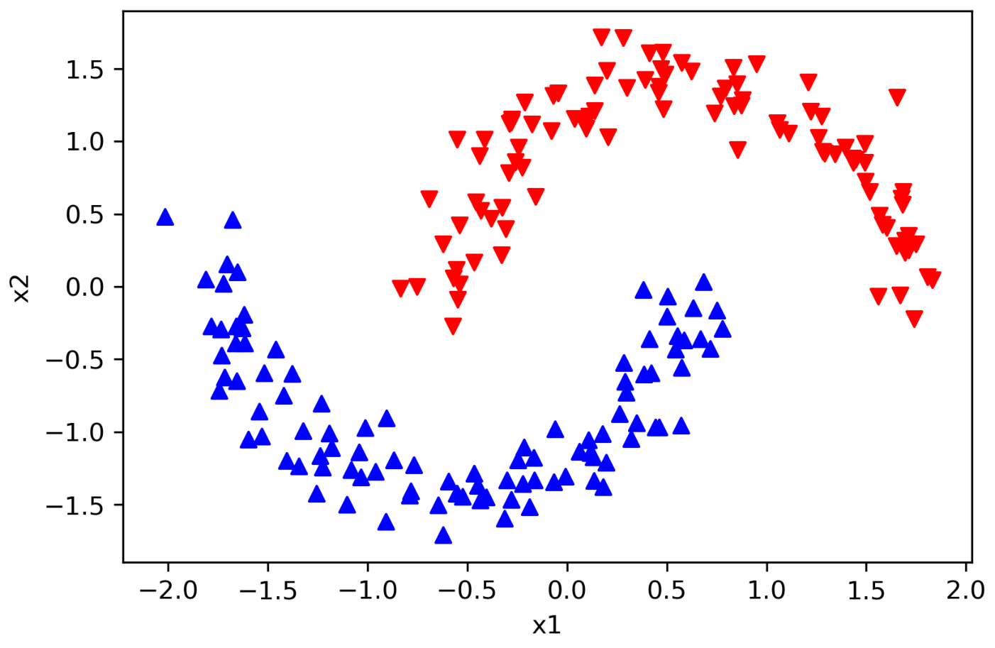
Refer to caption Refer to caption
(a) plot of dataset (b) CC with uniform weight
Refer to caption Refer to caption
(c) CC with Gaussian weight (d) NTL
Figure 3: Datasets and cluster path of centroids for half moons.

Next, using several real data sets 33 3 Datasets from scikit-learn https://scikit-learn.org/stable/datasets/index.html. The digit dataset was resampled so that n=500,100,50n=500,100,50., we quantitatively compared the quality of clustering on the basis of Adjusted Rand Index [11] (ARI for short; see, e.g., Vinh et al. 2010 for the details). ARI takes a value between 0 and 1, and when it is closer to 1, the clustering performance is considered to be higher.

For weights for CC, we consider the following two cases:

w{i,j}1={exp⁡(−0.5​‖ai−aj‖22),if ​i∈NN⁡(j,⌈n2⌉)​ or ​j∈NN⁡(i,⌈n2⌉),0,otherwise\displaystyle w^{1}_{\{i,j\}}=\left\{\begin{array}[]{ll}\exp(-0.5{\|a_{i}-a_{j}\|}_{2}^{2}),&\mbox{if }i\in\mathrm{NN}(j,\left\lceil\frac{n}{2}\right\rceil)\mbox{ or }j\in\mathrm{NN}(i,\left\lceil\frac{n}{2}\right\rceil),\\ 0,&\mbox{otherwise}\end{array}\right.

and

w{i,j}2={exp⁡(−0.5​‖ai−aj‖22),if ​i∈NN⁡(j,⌈n10⌉)​or​j∈NN⁡(i,⌈n10⌉),0,otherwise,\displaystyle w^{2}_{\{i,j\}}=\left\{\begin{array}[]{ll}\exp(-0.5{\|a_{i}-a_{j}\|}_{2}^{2}),&\mbox{if }i\in\mathrm{NN}(j,\left\lceil\frac{n}{10}\right\rceil)\ \mathrm{or}\ j\in\mathrm{NN}(i,\left\lceil\frac{n}{10}\right\rceil),\\ 0,&\mbox{otherwise},\end{array}\right.

where ⌈l⌉\lceil l\rceil denotes the smallest integer no less than ll. Note that (w{i,j}2){i,j}∈ℰ(w^{2}_{\{i,j\}})_{\{i,j\}\in\mathcal{E}} put more zeros on edges than (w{i,j}1){i,j}∈ℰ(w^{1}_{\{i,j\}})_{\{i,j\}\in\mathcal{E}}. Other settings are the same as in the previous (half-moon) example.

Table 1 summarizes the largest values of ARI along the cluster paths. We see from the table that weighted CC with w2w^{2} performed best for three data sets, as Theorem 1 implies. On the other hand, NTL recorded the best performance with the two datasets. While it cannot be said that one is better than the other, it is clear from this experiment that if prior information is not available, CC results in poor performance.

Table 1: Maximum Adjusted Rand Index through the cluster path.
iris wine digits (n=500n=500) digits (n=100n=100) digits (n=50n=50)
CC (uniform) 0.0015 0.0000 0.0082 0.0014 0.0013
CC (w1w^{1}) 0.5681 0.7577 0.5302 0.4577 0.3812
CC (w2w^{2}) 0.5681 0.7994 0.5346 0.5101 0.4443
NTL 0.5778 0.8260 0.3967 0.4134 0.4207

The best value for each data set is shown in boldface.

5.3 Piecewise constant fitting

As the final example, we consider the problem of recovering a piecewise constant signal from a noisy signal [5, Example 9.16] by using NL and NTL. Specifically, we consider a situation where n=1000n=1000 noisy signals x^1,…,x^1000∈ℝ\hat{x}_{1},...,\hat{x}_{1000}\in\mathbb{R} are generated as x^i=xio+ei\hat{x}_{i}=x_{i}^{\text{o}}+e_{i} with xox^{\rm o} being given as the original signal given as the black stepwise function in Figure 4 and eie_{i} being independently drawn from a normal distribution N⁡(0,0.22)N(0,{0.2}^{2}). Given the time series structure, we set 𝒱={1,…,1000}\mathcal{V}=\{1,...,1000\}, ℰ={{i,i+1}∣i,i+1∈𝒱}\mathcal{E}=\left\{\{i,i+1\}\mid i,i+1\in\mathcal{V}\right\}, fi​(xi)=12​(xi−x^i)2f_{i}(x_{i})=\frac{1}{2}{(x_{i}-\hat{x}_{i})}^{2}, and

D:=(1−10⋯001−1⋱⋮⋮⋱⋱⋱00⋯01−1).\displaystyle D:=\left(\begin{array}[]{ccccc}1&-1&0&\cdots&0\\ 0&1&-1&\ddots&\vdots\\ \vdots&\ddots&\ddots&\ddots&0\\ 0&\cdots&0&1&-1\end{array}\right).

It is known that σ:=λmin​(D​D⊤)=2​(1−cos⁡(π1000))≈9.87×10⁻⁶\sigma:=\lambda_{\min}(DD^{\top})=2(1-\rm{cos}(\frac{\pi}{1000}))\approx 9.87\times 10^{-6} [14, Theorem 2.2]. In this example, we consider not only the perspective of the cluster recovery but also the quality of the solution. The quality of the solution here means the closeness of the recovered signal and the original signal, i.e., ‖𝒙∗−𝒙o‖2\|\bm{x}^{*}-\bm{x}^{\text{o}}\|_{2}.

For NL, we computed the cluster path of centroids for γ∈{10−3×(1.2)t−1}t=1100\gamma\in\{10^{-3}\times(1.2)^{t-1}\}_{t=1}^{100} with the initial points 𝒚0=0,xi0=x^i\bm{y}^{0}=0,x_{i}^{0}=\hat{x}_{i} and the prior information w{i,i+1}=exp⁡(−0.5​‖x^i−x^i+1‖22)w_{\{i,i+1\}}=\exp(-0.5{\|\hat{x}_{i}-\hat{x}_{i+1}\|}_{2}^{2}). As for NTL, we applied ADMM from the same initial point, using K=5K=5 and γ=3​n​maxi​‖x^i‖2×1.001\gamma=3n\max_{i}{\|\hat{x}_{i}\|}_{2}\times 1.001. As an alternative heuristic for the cluster path algorithm, the initial value of ρ\rho was set to 11 though Examples 2 and 5 suggest setting as ρ>max⁡{2σ,1σ}=2σ>2×10⁵\rho>\max\{\frac{2}{\sigma},\frac{1}{\sigma}\}=\frac{2}{\sigma}>2\times 10^{5}. The parameter was updated by the formula ρ←min⁡{10​ρ,20.99​σ}\rho\leftarrow\min\{10\rho,\frac{2}{0.99\sigma}\} every 100 iterations. This modification is motivated by a similar heuristic used in Li and Pong 2015.

Figure 4 shows how well NL and NTL recover the original signal, which is denoted by black solid line, from the noisy signal, which is shown by the red solid line in the upper left panel. Since there is a degree of freedom in the evaluation criteria, two best-case results are given for NL. The panel (c) is the best in solution quality in the sense that the smallest value of ‖𝒙∗−𝒙o‖2\|\bm{x}^{*}-\bm{x}^{\text{o}}\|_{2} was attained out of 100 values of γ\gamma. On the other hand, the panel (d) is the best in the cardinality in the sense that the employed γ\gamma is the smallest out of the 100 values such that the number of jumped points is less than 5, which is the number of jumps in the original signal. We see from the panel (d) of Figure 4 that NL detected the jump points almost exactly as Theorem 1 implies, but the levels of the piecewise constants are far from the original signal. We think this is due to the fact that the degree of each node is at most 2, so that prior information was not given enough to recover the signal by NL. Employing more zero-weights as prior information worked better in the experiment of the previous subsection, but this example indicates that that is not always true. This indicates that it is not easy to give weights adequately for NL in advance. On the other hand, NTL not only detects the jump accurately but also estimates the levels of the piecewise constant more accurately than the best case of NL (lower left panel).
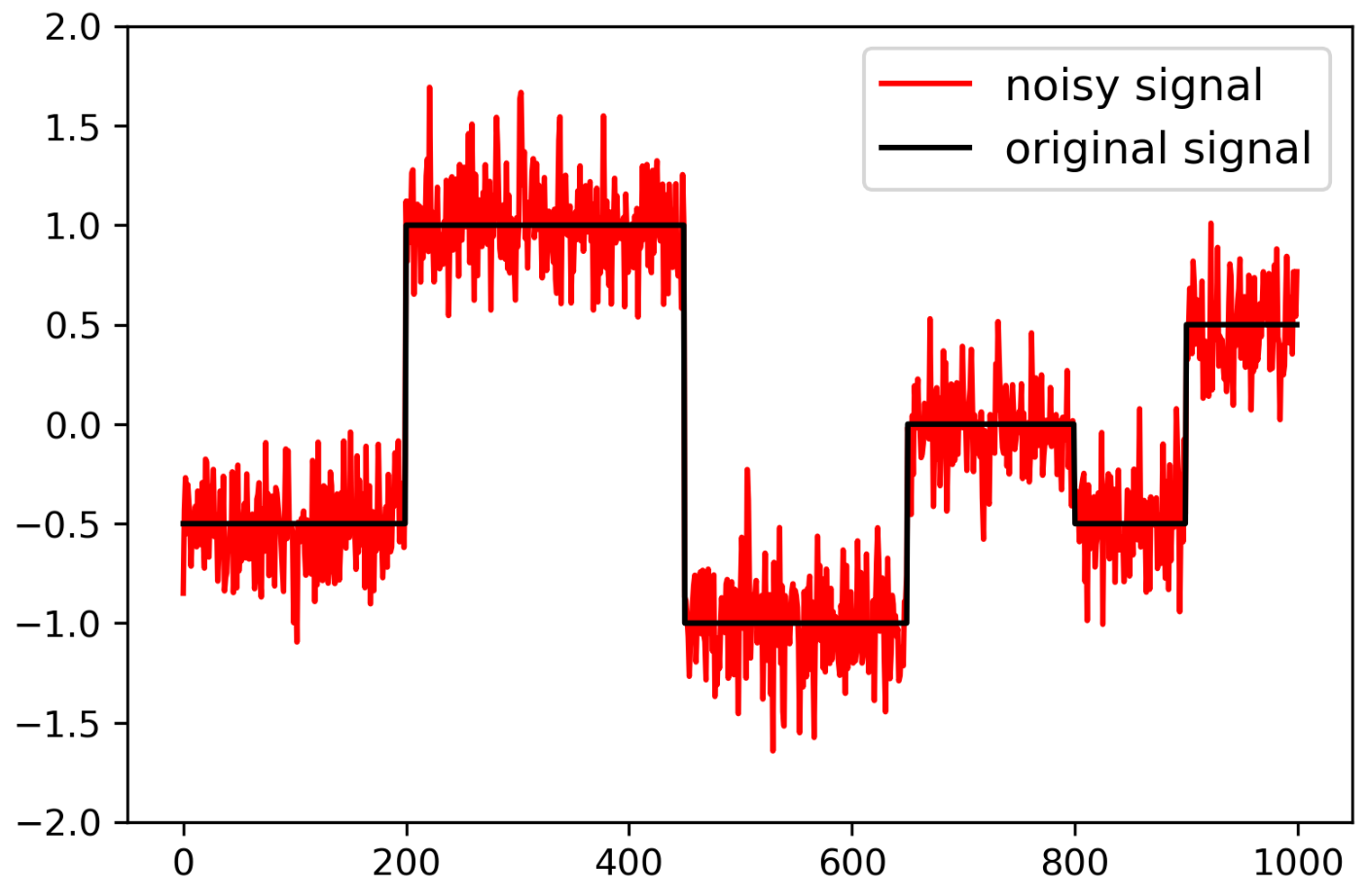
Refer to caption Refer to caption
(a) plot of dataset (b) NTL
Refer to caption Refer to caption
(c) NL (best in terms of quality) (d) NL (best in terms of cluster recovery)
Figure 4: Noisy signal and recovered signals.

6 Concluding remarks

In this paper, we study the cluster structure of Network Lasso (NL) from a couple of different angles. First, we derive a condition under which NL can recover (unseen) true clusters. Second, to obtain clusters that might not be attained by NL, we consider a cardinality-constraint on the number of unmerged pairs of centroids and show an equivalent unconstrained reformulation called Network Trimmed Lasso (NTL). Numerical examples demonstrate how NTL performs better than the ordinary NL, especially when any prior information is not available. These results suggest that we should use NL if we are given sufficient prior information, and use NTL otherwise. We also show the convergence of ADMM to a locally optimal solution of NTL or the cardinality-constrained problem. However, when the underlying graph is dense and large, the employed algorithm based on ADMM would lead to an impractical solution time. For example, when the graph is a complete graph, i.e., ℰ={{i,j}∣i≠j,i,j∈𝒱}\mathcal{E}=\left\{\{i,j\}\mid i\neq j,i,j\in\mathcal{V}\right\}, ADMM has to deal with n⁡(n−1)2​p\frac{n(n-1)}{2}p-dimension vectors, which would be prohibitively large even for a moderate nn, say, n=1000n=1000. Developing an efficient algorithm for such large data sets is left for future research.

Acknowledgments

Jun-ya Gotoh is supported in part by JSPS KAKENHI Grant 19H02379, 19H00808, and 20H00285.

References

  • Amir et al. [2020] Tal Amir, Ronen Basri, and Boaz Nadler. The trimmed lasso: Sparse recovery guarantees and practical optimization by the generalized soft-min penalty. arXiv preprint arXiv:2005.09021, 2020.
  • Beck [2017] Amir Beck. First-order methods in optimization. SIAM, 2017.
  • Bertsimas et al. [2017] Dimitris Bertsimas, Martin S Copenhaver, and Rahul Mazumder. The trimmed lasso: Sparsity and robustness. arXiv preprint arXiv:1708.04527, 2017.
  • Boyd et al. [2011] Stephen Boyd, Neal Parikh, Eric Chu, Borja Peleato, Jonathan Eckstein, et al. Distributed optimization and statistical learning via the alternating direction method of multipliers. Foundations and Trends® in Machine learning, 3(1):1–122, 2011.
  • Calafiore and El Ghaoui [2014] Giuseppe C. Calafiore and Laurent El Ghaoui. Optimization Models. Cambridge University Press, 2014.
  • Chi and Lange [2015] Eric C Chi and Kenneth Lange. Splitting methods for convex clustering. Journal of Computational and Graphical Statistics, 24(4):994–1013, 2015.
  • Cui et al. [2018] Ying Cui, Jong-Shi Pang, and Bodhisattva Sen. Composite difference-max programs for modern statistical estimation problems. SIAM Journal on Optimization, 28(4):3344–3374, 2018.
  • Gotoh et al. [2018] Jun-ya Gotoh, Akiko Takeda, and Katsuya Tono. Dc formulations and algorithms for sparse optimization problems. Mathematical Programming, 169(1):141–176, 2018.
  • Hallac et al. [2015] David Hallac, Jure Leskovec, and Stephen Boyd. Network lasso: Clustering and optimization in large graphs. In Proceedings of the 21th ACM SIGKDD international conference on knowledge discovery and data mining, pages 387–396, 2015.
  • Hocking et al. [2011] Toby Dylan Hocking, Armand Joulin, Francis Bach, and Jean-Philippe Vert. Clusterpath an algorithm for clustering using convex fusion penalties. In Proceedings of the 28th International Conference on Machine Learning, pages 745–752, 2011.
  • Hubert and Arabie [1985] Lawrence Hubert and Phipps Arabie. Comparing partitions. Journal of Classification, 2:193–218, 1985.
  • Jung and Tran [2019] Alexander Jung and Nguyen Tran. Localized linear regression in networked data. IEEE Signal Processing Letters, 26(7):1090–1094, 2019.
  • Jung et al. [2018] Alexander Jung, Nguyen Tran, and Alexandru Mara. When is network lasso accurate? Frontiers in Applied Mathematics and Statistics, 3(28):1–11, 2018.
  • Kulkarni et al. [1999] Devadatta Kulkarni, Darrell Schmidt, and Sze-Kai Tsui. Eigenvalues of tridiagonal pseudo-toeplitz matrices. Linear Algebra and its Applications, 297:63–80, 1999.
  • Li and Pong [2015] Guoyin Li and Ting Kei Pong. Global convergence of splitting methods for nonconvex composite optimization. SIAM Journal on Optimization, 25(4):2434–2460, 2015.
  • Lindsten et al. [2011] Fredrik Lindsten, Henrik Ohlsson, and Lennart Ljung. Clustering using sum-of-norms regularization: With application to particle filter output computation. In 2011 IEEE Statistical Signal Processing Workshop (SSP), pages 201–204, 2011.
  • Lu and Li [2018] Zhaosong Lu and Xiaorui Li. Sparse recovery via partial regularization: Models, theory, and algorithms. Mathematics of Operations Research, 43(4):1290–1316, 2018.
  • Panahi et al. [2017] Ashkan Panahi, Devdatt Dubhashi, Fredrik D Johansson, and Chiranjib Bhattacharyya. Clustering by sum of norms: Stochastic incremental algorithm, convergence and cluster recovery. In Proceedings of the 34th International Conference on Machine Learning-Volume 70, pages 2769–2777, 2017.
  • Pelckmans et al. [2005] Kristiaan Pelckmans, Joseph De Brabanter, Johan AK Suykens, and B De Moor. Convex clustering shrinkage. In PASCAL Workshop on Statistics and Optimization of Clustering Workshop, 2005.
  • Sun et al. [2021] Defeng Sun, Kim-Chuan Toh, and Yancheng Yuan. Convex clustering: Model, theoretical guarantee and efficient algorithm. Journal of Machine Learning Research, 22(9):1–32, 2021.
  • Vinh et al. [2010] Nguyen Xuan Vinh, Julien Epps, and James Bailey. Information theoretic measures for clusterings comparison: Variants, properties, normalization and correction for chance. Journal of Machine Learning Research, 11(95):2837–2854, 2010.
  • Yuan and Lin [2006] Ming Yuan and Yi Lin. Model selection and estimation in regression with grouped variables. Journal of the Royal Statistical Society: Series B (Statistical Methodology), 68(1):49–67, 2006.
  • Zhu et al. [2014] Changbo Zhu, Huan Xu, Chenlei Leng, and Shuicheng Yan. Convex optimization procedure for clustering: Theoretical revisit. In Advances in Neural Information Processing Systems 27, pages 1619–1627, 2014.