Clustering high dimensional meteorological scenarios: results and performance index
Abstract
The Reseau de Transport d’Electricité (RTE) is the French main electricity network operational manager and dedicates large number of resources and efforts towards understanding climate time series data. We discuss here the problem and the methodology of grouping and selecting representatives of possible climate scenarios among a large number of climate simulations provided by RTE. The data used is composed of temperature times series for 200 different possible scenarios on a grid of geographical locations in France. These should be clustered in order to detect common patterns regarding temperatures curves and help to choose representative scenarios for network simulations, which in turn can be used for energy optimisation. We first show that the choice of the distance used for the clustering has a strong impact on the meaning of the results: depending on the type of distance used, either spatial or temporal patterns prevail. Then we discuss the difficulty of fine-tuning the distance choice (combined with a dimension reduction procedure) and we propose a methodology based on a carefully designed index.
Keywords: clustering; temperature time series; performance index
1 Introduction
Temperature fluctuations have a strong influence on the electric consumption. As a consequence, identifying and finding groups of possible climate scenarios is useful for the analysis of mitigation and adaptation policies of the electric supply system [Li et al., 2018]. Given a set of time series representing temperature, a climate segmentation can potentially lead to a simplification of the posterior energy consumption analysis.
The work done by [Mougeot et al., 2018] focused on finding homogeneous climate regions in the French territory, that is, finding groups of geographical points with similar temperature time series. Without explicitly including in the model the spatial relationships between the time series, they were able to recover the French territory regions. Other authors, like [Sathiaraj et al., 2018] for the USA climate types and [Hidalgo and Jougla, 2018] for Toulouse have used different clustering techniques for the same purpose. A methodology for classifying the land surface into climate types using several climate variables, not only temperature series, was proposed by [Netzel and Stepinski, 2016].
Clustering is an unsupervised learning technique aiming at finding patterns (usually groups) in unlabeled data set. In the present case, clustering algorithms will be used to find homogeneous (in a sense to be defined carefully) groups of times series. As it is well known, the dimensionality of the data can be a formidable obstacle to the clustering techniques, due in great part to the phenomenon of concentration of measures in high dimension [Vershynin, 2018]: as the dimension grows, the usual distance (say L2) between two uniformly chosen data points concentrates around a constant value, making the identification of groups much more difficult. As a consequence, the main challenge when using clustering algorithms is to jointly choose a distance measure and a dimension reduction technique to break the concentration of distances. In the case of time series, the dimension (being the number of time points) is naturally high and these choices become particularly crucial.
On the other hand, given the spatio-temporal nature of our data set, the choice of the distance has strong implications in terms of "feature selections", i.e. on the specific patterns that will influence the clustering results. As it turns out, a detailed study of the choice of the distance effects on the data set needs to be undertaken. Otherwise, the final clustering results could be of little relevance for the practitioner.
Related work
Several recent review papers give a good account of the important body of literature on time series clustering in the last two decades (see for instance [Aghabozorgi et al., 2015]). On the one hand, there has been interesting work on finding new distances tailored to compare time-series (e.g. [Paparrizos and Gravano, 2015, Berndt and Clifford, 1994]), which allow to adapt clustering techniques to the particularities of time-ordered signals. Such distances have been showed to be relevant for many use cases where interesting patterns are present at an intermediate time scale, see e.g. [Yang et al., 2017]. However, there is generally no clear consensus regarding the best performing one, as it seems to depend on the domain of application.
On the other hand, many recent papers deal with the notion of deep clustering (see [Xie et al., 2016, Dizaji et al., 2017] and the survey [Min et al., 2018]) where the idea is to mimic a supervised methodology by choosing jointly a transformation of the data and a clustering procedure to minimize a loss function. This line of research has been shown to have very high performance e.g. in some imaging, computer vision and spatio-temporal applications [Wang et al., 2019]. However, as with many deep clustering techniques, a central issue might be the interpretability of the results and some difficult fine-tunning might be necessary to find interesting patterns [Min et al., 2018]. These issues become critical in our setting where the basic ingredients (distance and data transformation allowed) might distort completely the results. Though a promising research direction, we believe that many elements (in particular the impact of the distance and the dimension reduction) have to been studied first to obtain efficient and meaningful results. As a consequence, we decided to put our efforts in this first study on decoupling the data transformations and the clustering tasks, keeping a very simple clustering method and using an interpretable index to evaluate jointly both objectives to gain understanding on the effect of varying distances and transformations.
Data and objectives
The data that we are considering in this work are time series of hourly measured temperatures over a grid of geographical points in France and neighboring areas. These series have data for 200 years, each of which can be considered a different climate scenario. The Réseau de Transport d’Electricité (RTE) is the electricity transmission system operator of France. RTE, as other energy players have for many years expressed their needs for long series of data representative of the climate, scanning a maximum of possible hazards. Constant climate scenarios should be interpreted as sets of possible achievements of 200 years under the same climate. These are neither re-analyzes of past situations nor forecasts. Long simulated climate data series provide a vast sample of meteorological situations. In other words, for each geographical location, 200 temperature time series representing 200 temperature scenarios are available. On the one hand it is difficult to pretend that all these scenarios appear with equal probability. On the other hand, there is no real tool to have a precise idea on the probability of each scenario. Hence a more realistic technological advance towards this evaluation is to find groups of scenarios.
Contribution
Our task consists both in finding clusters of interest for the experts, but also in explaining in which sense they are appropriate. Observe that we actually deal with an intrinsically multi-objective problem where the efficiency of the clustering algorithm (in terms of, e.g., minimising the intra-cluster distances and maximizing the inter-cluster distances) has to be considered jointly with a penalization on the dimension reduction. Indeed, as it is intuitive, a drastic dimension might strongly deteriorate the meaningfulness of the final results. We will further show that even a mild dimension reduction might have far-reaching consequences.
Our main contribution is then two-fold:
- •
On the one hand, we give an interpretation for our data set of the several types of distances / transformations used in the time series literature. We show in particular that there is a quite counter-intuitive phase transition when the amount of dimension reduction grows, in terms of spatial vs temporal effects on the distance between time-series. In other words, when drastically reducing the dimension, only the temporal effects (different scenarios associated to a given place) are dominating. When keeping the same amount of information, the spatial differences are dominating. Hence, depending on the subsequent purpose of the clustering results (e.g., defining climate homogeneous regions or defining representative scenarios), specific distances should be carefully picked and employed.
We believe that such conclusions are, to a certain extent, generalizable or at least meaningful to other data sets of time series.
- •
On the other hand, we actually perform clustering of climate scenarios using several clustering pipelines including choices of distances, transformation of the data and clustering algorithms. Apart from providing a partition into groups, we also provide in each group a “typical scenario”. This could be a very useful tool for expert interpretation of each specific group.
The fine-tuning of the choice of the distance/dimension reduction is done using a tailored-made index based on embedding ideas, and allowing to reach an appropriate trade-off between clustering efficiency (where dimension reduction plays a positive role) and data distorsion (where dimension reduction can play a negative role). This allows to partially validate our clustering results, in parallel of the validation provided by RTE experts. When the focus is put on clustering one-year-scenarios, we show that the best results are reached with the lagged correlation distance and to a minor extent with DTW.
The paper is organized as follows. Section 2 gives a description of the data provided by Meteo-France through RTE. Section 3 gives a review of the clustering techniques used in the paper, including data transformation, distance measures and clustering algorithms. Section 4.1 explains the qualitative properties of classical distances in our context and highlights a phase transitions in terms of spatial vs temporal explainability. Section 3.3 defines our comparison index. Section 4.2 conducts the clustering experiments in the meteorological data and gives indication on the performance of our comparison index. Section 5 gives conclusions and future lines of work.
2 Meteorological data
2.1 True data for forecasters and scenarios
Observation is the first step in a forecast. 90% of the observation data used by Meteo-France’s forecast models come from meteorological satellites. The remaining 10% are provided by ground stations, radiosonde, airborne and commercial vessel sensors, or installed on anchored and drifting buoys. Meteo-France also receives other meteorological services from measurements collected around the globe. All these observations are then processed to extract useful information towards the forecasting model: one speaks of data assimilation. About 22 million observations data are used every day by the models at the end of the assimilation step. The data from the observations are combined with other information, such as very recent forecasts, to establish an initial state of the atmosphere that the model will be able to use.
From this initial state, the models simulate the evolution of the atmosphere, which they cut into a grid in three dimensions with meshes of different sizes. Simulation is based on the physical laws that govern atmospheric evolution: mainly the laws of the mechanics of fluids, supplemented by those governing changes in the state of water (condensation, evaporation, precipitation formation), turbulence, radiation or the many interactions with the Earth’s surface and even space.
To describe the state of the atmosphere and to perform their calculations, the weather models cut the atmosphere into elementary boxes each containing a value of pressure, wind, temperature, humidity and others. On the horizontal, this decoupage is defined by the mesh distance of the grid of the model, and on the vertical, by the number of levels of the model. Mesh distance and number of levels vary according to the desired fineness, the computing power available, the vocation of the model (short-term forecast, climate simulation, seasonal forecast for instance).
For phenomena exceeding the size of their mesh, the models follow these physical laws in all rigor. On the other hand, smaller phenomena are not explicitly described in the model. They are taken into account by means of specific algorithms that simulate their average influence within the meshes of the model.
Note that the results of these simulations performed by the models are not forecast but scenarios of evolution of the main meteorological parameters in all the points of the grid which represents the atmosphere.
2.2 Scenarios
For points on a 76 x 51 grid, which includes all the French territory and surrounding areas, hourly measurements of temperature over a 200 year span are available, with each year representing a possible climate scenario.
The temperature measurements are available hourly over each geographical point and over a time span of 200 ‘years’. These daily observations are contiguous in that, for example, the last day of first year is followed by the first day of the second year. However, we will not use this contiguity information and each ‘year’ will be interpreted as a different possible climate scenario. This is what we mean in the following, whenever we refer to a climate scenario. Instead of studying the time series on the whole year we also decided to restrict to winters, which are crucial for energy providers.
So, in the sequel, we are considering the observation of 200 time-series of hourly observed temperatures on 90 days of winter, all corresponding to the same geographical point. As a preprocessing, we center each series by the global mean (considering all geographical points, all scenarios).
3 Methodology
For general clustering algorithms, four important choices enter into play :
- 1.
The representation of the data in the feature space (which can be the original space) and the dimension reduction to transform the original data into features.
- 2.
The distance used to measure dissimilarities between the representations of the data in the feature space and the distance used to measure dissimilarities between the original data.
- 3.
The number of clusters.
- 4.
The actual method to partition data points into clusters.
In what follows, we discuss several alternatives considered for these choices.
3.1 Representations and distances
This section concerns the first two points listed above as key factors of a clustering algorithm, by exhibiting various techniques we considered to represent the data and to compute distances between the representations.
3.1.1 Representations
PCA
Given a data set where each data point is in , the PCA algorithm produces a predetermined number of directions (the principal directions) on which to project the data points to best capture their variability. The resulting projections are the so called principal components. The number of principal components is chosen to explain at least of the variability in the data.
Functional approximation featuring
Another point of view consists in taking into account the fact that each data point is in fact a function of time observed at regular instances. We can represent , the temperature at a given point at time as a random variable of the form
for some error random variable and some mesh . The function can then be estimated in a nonparametric fashion using a dictionary of basis functions, see for instance [Tsybakov, 2008]. We will use two main dictionaries, the Haar basis and the Fourier basis taking as assumptions that the function is sufficiently smooth (for the Haar basis) or has some prominent frequencies such as day-night (in the case of the Fourier basis). The number of terms in the basis expansion is chosen to explain at least of the variability in the data.
3.1.2 Distances
Any clustering algorithm requires a notion of distances between the objects being grouped. This is actually the key ingredient of any clustering methodology. In our case, two time series corresponding to different locations and/or scenarios will be deemed ‘similar’ whenever their distance is ‘small’. Next, we list some of the notions of distance between time series that we considered useful. Let and be any two time series.
Euclidean
This is just the standard euclidean distance between two vectors, i.e., the distance is . Note that this does not take into account the dynamic nature of the data at all, but has demonstrated to be competitive in terms of accuracy [Paparrizos and Gravano, 2015].
Note that this euclidean distance is used in the data space or in the feature space when the data are represented by their projections (PCA, functional bases) or their autoencoder representatives
Max Lagged Pearson Correlation (MLPC)
The MLPC seeks for an optimal alignment between two signals, with the two series only being allowed to be aligned via shifts in the time axis. The distance between two times series and is defined as:
where is the Pearson correlation at lags and is a user-specified constant. The distance is always equal or greater than 0 and equal or less than 2.
This comparison has good properties for signal presenting similarities except for a fixed translation in time. This distance was inspired by the one proposed in [Paparrizos and Gravano, 2015], as part of the k-shape clustering algorithm.
Dynamic Time Warping
Introduced by [Berndt and Clifford, 1994], this distance essentially looks for the optimal, possibly non-linear, alignment between the two series. For details see [Berndt and Clifford, 1994]. [Sakoe and Chiba, 1978] proposed a constrained version with similar performance results but less computational complexity.
Note that both DTW and MLPC, unlike the traditional Euclidean distance, take into account the dynamic nature of the data, the fact that we are dealing with time series, which by their very definition can have lagged relations. Unlike the Max Lagged Pearson-Correlation, DTW allows for non-linear alignments of the series and is computationally more demanding.
The plots in Figure 1 illustrate how the DTW distance works. In the top panel we see a test series in red and the series closest to it in black; grey lines show the optimal alignment. In the bottom panel we see the test series in red and the series farthest from it in black; grey lines again show the optimal alignment. The series closest to the test series mainly differs in a small warping of the time axis. On the contrary, the series farthest from the test series has completely different dynamics. This is what the DTW distance seeks to capture. The following 3D interactive visualizations may help the rather gain further insights into DTW: https://plot.ly/˜aumfurer/2/closest, https://plot.ly/˜aumfurer/4/farthest.


We should mention that the added flexibility associated with DTW, namely, it allowing for non-linear alignments, comes with the price of a significant computational cost when compared to the Max Lagged Pearson-Correlation distance. As a matter of fact, the worst case complexity for computing DTW is , an order worse than the needed for the MLPC. Moreover, results obtained using the DTW distance can be much harder to interpret, due to that added flexibility.
3.2 Clustering method: K-Medoids
We now quickly present the simple clustering algorithms that is considered in our analysis. K-Medoids is a very commonly used clustering algorithm. It is an easily implementable and interpretable procedure which aims at producing a local minimum to the following problem: Given the number of clusters, find a partition of the data points into disjoint clusters such that the sum of the distances of members of a cluster to a ‘cluster representative’ is minimal. The optimisation problem is similar to K-means but unlike K-Means, cluster representatives in K-Medoids are data points whereas in K-means they are barycenters. The algorithm uses random starts, so the result of one run of the algorithm is a local minimum depending on this random starts. As a consequence, the algorithm has to be run a significant number of times to get a global minimum. See [Kaufman and Rousseeuw, 2009] for details. In practice, it works as follows. The centroids are randomly initialized at some data points. Each point in the data-set is then assigned to the centroid closest to it. Then, the centroids in each cluster are updated to the cluster members that minimize the sum of the distances to all other members of that cluster. Finally, each point is re-assigned to the cluster with the centroid closest to it. These two last steps are repeated until convergence.
K-means and K-Medoids often give comparable results. K-means exactly optimizes the euclidean distance, K-Medoids has good properties of robustness with respect to outliers.
We chose this clustering method among many others, because of various reasons : simplicity of implementation, control of the number of clusters (chosen in advance), statistical interpretation, stability (if the number of runs is important enough, and the number of clusters adequate) and the ease of interpretability of the clusters (since they have one representative which is a real point and not a barycenter).
3.3 Evaluation index
As usual in unsupervised learning, in the absence of ground truth, there is no direct way to detect results of poor quality i.e. far from the theoretical ’hypothetical’ one (as opposed to estimating a regression function for instance where the observed errors are giving hints).
In this section, we propose and explore a new evaluation methodology by defining an index measuring the trade-off between the faithfulness of the representation to the original data on the one hand and the clustering efficiency in the feature space on the other hand. The difference with e.g. loss functions introduced in some literature on deep clustering [Min et al., 2018] is the fact that this index can generalize to:
- •
any distances in the original and the features spaces,
- •
any transformation from the original to the feature space, (even when there is no well defined notion of best reconstruction).
Our index has two components and is trying to balance two opposed effects, standard in clustering : by reducing drastically the dimension we obtain a very stable clustering with generally very good measures of efficiency, but quite poor interest and interpretability since the representation of the data in the feature space is weak.
Faithfulness Our index is inspired by the stochastic neighbors embeddings related techniques. We start by defining a probability distribution using a Gaussian model for the embedding in the original space equipped with a basic distance (euclidean or k-shape or DTW) (see for instance [Maaten and Hinton, 2008] for the exact procedures). Then, we define a probability distribution on the feature space using a Gaussian distribution for the embedding since the dimension is expected to be still reasonably high except in some pathological cases. The intuition here is that should represent a high-dimensional space while should represent the "projection" into a lower (but still reasonably high) dimensional space.
Following classical approaches, we then define the distance between our evaluation distribution and our feature distribution , as the symmetrized Kullback-Leibler:
Since this metric gives a value between 0 and infinity, we will use a logistic function to restrict to the interval . Then our "Fidelity" measure is defined as:
The intuition here is that there should be some quite sharp transition (depending of the typical behavior of ) between faithful enough representations and unmeaningful ones.
Clustering efficiency and balance
On the other hand, we now define an index that we call the within index as an efficiency measure for the clustering in the feature space. We use an adaptation of classical clustering indices (for instance the Carinski-Harabasz index), which is convenient to measure the efficiency of the -medoid algorithm, as it corresponds to a normalized version of the functional optimized by the -medoid algorithm and which is defined as follows.
For a given clustering and for any time series , define as the center of the cluster assign to by this clustering.
Then the within index is simply the normalized ratio of the mean squared distances of series to their centers with the mean square distance between series:
Our final index combines in a multiplicative manner both measures:
This multiplicative structure (compared to more standard additive penalizations) is simply due to the exponential shape of our fidelity index.
4 Results
4.1 Significance of classical distances
To understand in depth the implication of the choice of the distance, we perform the following experiments. We choose a given geographical point in France for a particular year as a reference. That is, our reference time series corresponds to the temperatures for a latitude and longitude point in France for a particular scenario. This time series is compared with :
- A
Times series corresponding to the same geographical point along other scenarios (there are 198 other scenarios different from the reference one).
- B
Times series corresponding to other geographical points in France but the same scenario that the reference series (the geographical grid has more than 3500 points, but we compared it with 198 randomly chosen points so that the number of series in group B is the same than in group A).
This analysis was repeated for different geographical points and scenarios as reference time series, and the results were similar. We hence show the results of just one reference temperature times series. We compute the distances in table 1 between the reference series and series from group A (orange in figure 2) and between the reference time series and series from group B (blue in figure 2).
| Transformation | Distance | Name | ||
|---|---|---|---|---|
| plain time series | L2 | L2 | ||
| Haar, energy 0.95 | L2 | Haar95 | ||
| zscore | MLPC | MLPC | ||
| zscore | DTW | DTW | ||
| mean | L2 | Mean |
Figure 2 shows, for each considered distance, the distribution of the distances for the two groups of series described above. We can observe that, when using the mean, time series from group A are closer to the the reference series than series from group B. That is, mean temperatures in the reference times series are more similar along different scenarios than along geographical points in the same year. But, when considering distances that take into account the shape of the series the situation changes drastically. Figure 2 shows that Haar level 4 already has a similar distance distribution than Haar level 10, revealing that reducing to level 4 is sufficient for our purposes.


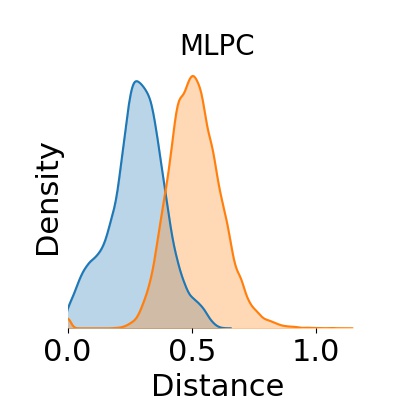
The blue distributions progressively shift to the right of the orange distributions, which means that distance of the series from group B to the reference one become progressively smaller than the ones from group A. In order to understand this behaviour, Figure 3(a) (upper left) displays the reference time series in gray while Figure 3(b) displays in orange the Haar level 5 representation of the times series corresponding to group A (same geographical point, different scenarios).
In 3(b), the mean of these time series is plotted in orange. Notice that although the shape of the representations are seemingly quite different, the mean temperatures are close to each other.
In 3(c), the same reference time series is displayed in gray, while the transformed Haar level 5 times series corresponding to group B (same scenario, different geographical points) are displayed in orange. In 3(d), we show their corresponding means. In this case, we observed that the means are further away from the mean of the reference series but at the same time, curves from 3 seem to have similar shapes.


We have hence underlined that the different distances considered lead to take into account different aspects of the temperature times series. Moreover, from this analysis, we evidenced that the climate scenarios are diverse in terms of shape (i.e., different scenarios display different shape for the same geographical point) while preserving the mean temperature (the same geographical point displays similar mean temperature along many scenarios).
In order to be able to understand the transition observed in figure 2, it is crucial to understand the characteristics of each of the considered distances.
In Figure 4, the distances are sorted according to which feature they highlight. On the left side, we consider the mean temperature, and on the right, the correlation. Keep in mind that Fourier and Haar representation, when having very high level of thresholding, agree with the mean, while they boil down to L2 in absence of thresholding.

4.2 Clustering time series for a fixed geographical location
We now discuss the practical choice of a distance and the resulting clustering using the previously explained methodology. In the sequel, we fix one geographical point and consider all the temperatures times series corresponding to the different scenarios for that point. In figure 5, all the z-normalized temperatures series corresponding to the chosen geographical point are displayed and it can be seen that there is no clear structure, except for the day-night variability.

Table 2 shows the different models we tried. Each model consists of a representation of the data, a distance and a clustering algorithm.
| Representation of data | Distance | Clustering method | Name |
|---|---|---|---|
| mean | L2 | k-medoids | mean |
| plain time series | L2 | k-medoids | L2 |
| Fourier | L2 | k-medoids | Fourier |
| Haar | L2 | k-medoids | Haar |
| PCA | L2 | k-medoids | PCA |
| zscore | max lagged pearson correlation | k-medoids | MLPC |
| zscore | DTW | k-medoids | DTW |
Each representation and distance is able, in principle, to capture different features of the data.
Representing a scenario with its annual mean is an oversimplification but is useful as a baseline for comparisons. PCA95, Fourier95 and Haar95 rely on a dimensional reduction, PCA based on the data itself and Fourier and Haar in the respective bases. On the other hand, MLCC and DTW are able to capture similarities regardless of shift and scale translations.
We kept the clustering method as simple as possible and chose k-medoids for all cases.
We first give evidence that consensus and within index are a poor overall performance choice in this context. Indeed, it gives a great advantage to drastic dimensional reduction, loosing the patterns that one is looking for a in the data.
Focusing on our new definition of performance index, we consider the following experiments. Given that k-medoids uses random points for the initial values of the centers, we perform several clustering runs (that is, run 5 times the corresponding clustering algorithm) and compute the mean index between the labeled outputs. Figure 8, 9, 10 show the index when using different metrics as references.
In this work, we did not focus on the important problem of selecting the number of clusters and simply set the number of clusters to 15, based on domain experts advice. Note however, that we performed the same experiments for different numbers and concluded our analysis and results stay valid for a range of cluster numbers close to 15.
While the consensus index does not give enough evidence to select any model, (and would lead eventually to choose the representation keeping only the means of the time series), our index allows to order conveniently the dimension reductions techniques and to naturally define a best one.
It is remarkable to note that in case of the underlying distance being max-lagged correlation or DTW, then this distance (without any dimension reduction on the signals) is clearly the best choice. In future work, it would be interesting to define new versions of both distances on modified versions of the time series incorporating a certain amount of dimension reduction. In the case of L2 however, reducing the dimension clearly pays off and there is a non trivial optimum.


4.2.1 Description of the clusters
Figure 11 and 12 shows four resulting clusters for the MLPC model out of 15 clusters. Figure 13 and 14 shows four resulting clusters out of 15 for the PCA95 model out of 15 clusters.
In each cluster, the cluster representative is in color (or thick black) and the other series that belong to that cluster are in gray. The representative is the barycenter of the cluster series. All the series in the cluster are lagged to maximize the correlation with the cluster barycenter. It can be clearly seen that there is common pattern among the series in each cluster and that the cluster representative in indeed reflecting the overall behavior of the cluster.


5 Conclusion
We explored the clustering of temperature time series and we showed that the distance employed by the clustering is crucial in terms of results interpretation and should be chosen with case in function of the spatio/temporal analysis undertaken. We then focused on clustering scenarios for a given location and showed that given a distance, well performing clustering can be chosen through maximizing an index balancing the trade-off between clustering efficiency and dimension reduction. Building on these conclusions, it would be interesting to revisit the loss functions proposed for deep clustering where the dimension reduction and the clustering are considered jointly.
References
- [Aghabozorgi et al., 2015] Aghabozorgi, S., Seyed Shirkhorshidi, A., and Ying Wah, T. (2015). Time-series clustering - a decade review. Inf. Syst., 53(C):16–38.
- [Berndt and Clifford, 1994] Berndt, D. J. and Clifford, J. (1994). Using dynamic time warping to find patterns in time series. In Proceedings of the 3rd International Conference on Knowledge Discovery and Data Mining, AAAIWS’94, pages 359–370. AAAI Press.
- [Dizaji et al., 2017] Dizaji, K. G., Herandi, A., and Huang, H. (2017). Deep clustering via joint convolutional autoencoder embedding and relative entropy minimization. CoRR, abs/1704.06327.
- [Hidalgo and Jougla, 2018] Hidalgo, J. and Jougla, R. (2018). On the use of local weather types classification to improve climate understanding: An application on the urban climate of toulouse. PLOS ONE, 13:e0208138.
- [Kaufman and Rousseeuw, 2009] Kaufman, L. and Rousseeuw, P. J. (2009). Finding groups in data: an introduction to cluster analysis, volume 344. John Wiley & Sons.
- [Li et al., 2018] Li, Y., A. Pizer, W., and wu, L. (2018). Climate change and residential electricity consumption in the yangtze river delta, china. Proceedings of the National Academy of Sciences, 116:201804667.
- [Maaten and Hinton, 2008] Maaten, L. v. d. and Hinton, G. (2008). Visualizing data using t-sne. Journal of machine learning research, 9(Nov):2579–2605.
- [Min et al., 2018] Min, E., Guo, X., Liu, Q., Zhang, G., Cui, J., and Long, J. (2018). A survey of clustering with deep learning: From the perspective of network architecture. IEEE Access, PP:1–1.
- [Mougeot et al., 2018] Mougeot, M., Picard, D., Lefieux, V., and Marchand, M. (2018). Homogeneous climate regions using learning algorithms. Springer Proceedings in Mathematics and Statistics vol 254.
- [Netzel and Stepinski, 2016] Netzel, P. and Stepinski, T. (2016). On using a clustering approach for global climate classification.
- [Paparrizos and Gravano, 2015] Paparrizos, J. and Gravano, L. (2015). k-shape: Efficient and accurate clustering of time series. In Proceedings of the 2015 ACM SIGMOD International Conference on Management of Data, pages 1855–1870. ACM.
- [Sakoe and Chiba, 1978] Sakoe, H. and Chiba, S. (1978). Dynamic programming algorithm optimization for spoken word recognition. IEEE transactions on acoustics, speech, and signal processing, 26(1):43–49.
- [Sathiaraj et al., 2018] Sathiaraj, D., Huang, X., and Chen, J. (2018). Predicting climate types for the continental united states using unsupervised clustering techniques. Wiley.
- [Tsybakov, 2008] Tsybakov, A. B. (2008). Introduction to Nonparametric Estimation. Springer Publishing Company, Incorporated, 1st edition.
- [Vershynin, 2018] Vershynin, R. (2018). High-Dimensional Probability: An Introduction with Applications in Data Science. Cambridge Series in Statistical and Probabilistic Mathematics. Cambridge University Press.
- [Wang et al., 2019] Wang, S., Cao, J., and Yu, P. S. (2019). Deep learning for spatio-temporal data mining: A survey. CoRR, abs/1906.04928.
- [Xie et al., 2016] Xie, J., Girshick, R., and Farhadi, A. (2016). Unsupervised deep embedding for clustering analysis. In Balcan, M. F. and Weinberger, K. Q., editors, Proceedings of The 33rd International Conference on Machine Learning, volume 48 of Proceedings of Machine Learning Research, pages 478–487, New York, New York, USA. PMLR.
- [Yang et al., 2017] Yang, J., Ning, C., Zhang, F., Deb, C., Cheong, K., Lee, S., Sekhar, C., and Tham, K. (2017). K-shape clustering algorithm for building energy usage patterns analysis and forecasting model accuracy improvement. Energy and Buildings, 146.