The volume of the boundary of a Sobolev $(p,q)$ -extension domainThanks: The first and third authors have been supported by the Academy of Finland (project No. 323960). The third author thanks Tero Kilpeläinen for introducing him to fine topology.

Pekka Koskela, Alexander Ukhlov and Zheng Zhu Address: Pekka Koskela
Department of Mathematics and Statistics
University of Jyväskylä, P.O. Box 35 (MaD), FI-40014, Jyväskylä, Finland Email address: pekka.j.koskela@jyu.fi Address: Alexander Ukhlov
Department of Mathematics
Ben Gurion University of the Negev, P.O.B. 653, Be’er Sheva 84105, Israel Email address: ukhlov@math.bgu.ac.il Address: Zheng Zhu
Department of Mathematics and Statistics
University of Jyäskylä, P.O. Box 35 (MaD), FI-40014, Jyväskylä, Finland Email address: zheng.z.zhu@jyu.fi

Abstract.

Let $n\geq 2$ and $1\leq q<p<\infty$ . We prove that if ${\Omega}\subset{{{\mathbb{R}}}^{n}}$ is a Sobolev $(p,q)$ -extension domain, with additional capacitory restrictions on boundary in the case $q\leq n-1$ , $n>2$ , then $|\partial{\Omega}|=0$ . In the case $1\leq q<n-1$ , we give an example of a Sobolev $(p,q)$ -extension domain with $|\partial{\Omega}|>0$ .

2010 Mathematics Subject Classification

46E35, 30L99

1. Introduction

Let $1\leq q\leq p\leq\infty$ . Then a bounded domain ${\Omega}\subset{{{\mathbb{R}}}^{n}}$ , $n\geq 2$ , is said to be a Sobolev $(p,q)$ -extension domain if there exists a bounded extension operator

E:W^{1,p}({\Omega})\to W^{1,q}({{{\mathbb{R}}}^{n}}).

Partial motivation for the study of Sobolev extensions comes from PDEs (see, for example, [25]). In [2, 33] it was proved that if $\Omega\subset\mathbb{R}^{n}$ is a Lipschitz domain, then there exists a bounded linear extension operator $E:W^{k,p}(\Omega)\to W^{k,p}(\mathbb{R}^{n})$ , for each $k\geq 1$ and all $1\leq p\leq\infty$ . Here $W^{k,p}({\Omega})$ is the Banach space of $L^{p}$ -integrable functions whose weak derivatives up to order $k$ belong to $L^{p}(\Omega)$ . More generally, the notion of $(\varepsilon,\delta)$ -domains was introduced in [15] and it was proved that, for every $(\varepsilon,\delta)$ -domain there exists a bounded linear extension operator $E:W^{k,p}(\Omega)\to W^{k,p}(\mathbb{R}^{n})$ , for all $k\geq 1$ and $1\leq p\leq\infty$ .

A geometric characterization of simply connected planar Sobolev $(2,2)$ -extension domains was obtained in [40]. By later results in [17, 19, 20, 30], we understand the geometry of simply connected planar Sobolev $(p,p)$ -extension domains, for all $1\leq p\leq\infty$ . Geometric characterizations are also known in the case of homogeneous Sobolev spaces $L^{k,p}(\Omega)$ , $2<p<\infty$ , defined on simply connected planar domains. Here $L^{k,p}({\Omega})$ is the seminormed space of locally integrable functions whose $k$ th-order distributional partial derivatives belong to $L^{P}({\Omega})$ . However, no characterizations are available in the general setting.

The boundary $\partial{\Omega}$ of a Sobolev $(p,p)$ -extension domain is necessarily of volume zero when $1\leq p<\infty$ by results in [9]. Actually, ${\Omega}$ has to be Ahlfors regular in the sense that

(1.1)

|B(x,r)\cap{\Omega}|\geq C|B(x,r)|

for every $x\in\partial\Omega$ and all $0<r<\min\{1,\frac{1}{4}{\mathop{\mathrm{}}{\,diam\,}}{\Omega}\}$ with a constant $C$ independent of $x,r$ . Even more is known if $\Omega$ is additionally a planar Jordan domain. In this case $\Omega$ has to be a so-called John domain when $1\leq p\leq 2$ and the complementary domain needs to be a John domain when $2\leq p<\infty$ . Consequently, the Hausdorff dimension of $\partial{\Omega}$ is necessarily strictly less than two by results in [21]. For a sharp estimate see the very recent paper [24]. However, in general, the Hausdorff dimension of the boundary of a Sobolev $(p,p)$ -extension domain ${\Omega}\subset{{{\mathbb{R}}}^{n}}$ can well be $n$ .

Much less is known when $q<p$ . First of all, no geometric criteria is available even when ${\Omega}$ is planar and Jordan. The only existing result related to (1.1) is the generalized Ahlfors-type estimate

(1.2)

\Phi(B(x,r))^{p-q}|B(x,r)\cap\Omega|^{q}\geq C|B(x,r)|^{p}

from [36] (also see [37]) for the case $n<q<p<\infty$ . Here $\Phi$ is a bounded, monotone and countably additive set function, defined on open sets $U\subset{{{\mathbb{R}}}^{n}}$ with $U\cap{\Omega}\neq\emptyset$ . It is generated by the extension property. By differentiating $\Phi$ with respect to the Lebesgue measure, one concludes that $|\partial{\Omega}|=0$ if ${\Omega}$ is a Sobolev $(p,q)$ -extension domain with $n<q<p<\infty$ .

Our first result gives the optimal capacitory version of (1.2) for the full scale $1\leq q<p<\infty$ . Towards the statement, we set $A(x;s,t)=B(x,t)\setminus B(x,s)$ when $x\in{{{\mathbb{R}}}^{n}}$ and $0<s<t.$

Theorem 1.1.

Let ${\Omega}\subset{{{\mathbb{R}}}^{n}}$ be a Sobolev $(p,q)$ -extension domain with $1\leq q<p<\infty$ . Then there exists a nonnegative, bounded, monotone and countably additive set function $\Phi$ , defined on open sets, such that, for every $x\in\partial{{\Omega}}$ and each $0<r<\min\{1,\frac{1}{4}{\mathop{\mathrm{}}{\,diam\,}}({\Omega})\}$ , we have

(1.3)

\Phi(B(x,r))^{p-q}|B(x,r)\cap{\Omega}|^{q}\geq r^{pq}Cap_{q}\left({\Omega}\cap B\left(x,\frac{r}{4}\right),{\Omega}\cap A\left(x;\frac{r}{2},\frac{3r}{4}\right);B(x,r)\right)^{p}.

Here $Cap_{q}$ is the classical variational $q$ -capacity.

Since the lower bound in (1.3) comes with a term related to the capacitory size of a portion of ${\Omega}$ , let us analyze it carefully in the model case of an exterior spire of doubling order. More precisely, let $w:[0,\infty)\to[0,\infty)$ be continuous, increasing and differentiable with $w(0)=0$ , $w(1)=1$ and so that $w(2t)\leq Cw(t)$ for all $t>0$ . We also require $w^{\prime}$ to be increasing on $(0,1)$ with $\lim_{t\to 0^{+}}w^{\prime}(t)=0.$ We define

(1.4)

{\Omega}^{n}_{w}:=\{z=(t,x)\in{\mathbb{R}}\times{\mathbb{R}}^{n-1}:0<t\leq 1,|x|<w(t)\}\cup B^{n}((2,0),\sqrt{2}).

See Figure $1$ . We call ${\Omega}^{n}_{w}$ an outward cusp domain with a doubling cusp function $w$ . The boundary of ${\Omega}^{n}_{w}$ contains an exterior spire of order $w$ at the origin.

Refer to caption — Figure 1. An outward cuspidal domain.

We write $A\sim_{c}B$ if $\frac{1}{c}A\leq B\leq cA$ for a constant $c>1$ . The following theorem gives the sharp capacitory estimate at the origin for the outward cusp domain ${\Omega}^{n}_{w}$ .

Theorem 1.2.

Let $n\geq 3,$ and let ${\Omega}^{n}_{w}\subset{{{\mathbb{R}}}^{n}}$ be an outward cusp domain with a doubling cusp function $w$ . Then, for every $0<r<1$ , we have

(1.5)

Cap_{p}\left({\Omega}^{n}_{w}\cap B\left(0,\frac{r}{4}\right),{\Omega}^{n}_{w}\cap A\left(0;\frac{r}{2},\frac{3r}{4}\right);B(0,r)\right)\sim_{c}\\ Cap_{p}\left({\Omega}^{n}_{w}\cap B\left(0,\frac{r}{4}\right),A\left(0;\frac{r}{2},\frac{3r}{4}\right);B(0,r)\right)\sim_{c}\\ \begin{cases}r^{n-p}&\textnormal{if }\ n-1<p<\infty\\ \frac{r}{\log^{n-2}\frac{r}{w(r)}}&\textnormal{if }\ p=n-1\\ r(w(r))^{n-1-p}&\textnormal{if }\ 1\leq p<n-1\end{cases}

where the constant $c$ is independent of $r$ .

The $(p,q)$ -extendability properties for the domains ${\Omega}^{n}_{w}$ are known by [26, 27, 28, 29]. We show in Section 5 that these domains give examples of settings where the exponents in (1.3) are optimal and where boundedness of $\Phi$ cannot be replaced, say, by an estimate of the type $\Phi(B(x,r))\leq Cr^{\alpha}.$ Besides of boundedness, the other crucial property of our set function $\Phi$ is additivity. It allows one to obtain better volume estimates when the center of $B(x,r)$ does not belong to a suitable exceptional set. These estimates are shown to be sharp in Section 5 for wedges generated by ${\Omega}^{n}_{w}.$

In order to effectively use (1.3), one needs an estimate for the respective capacitory term. For this, we employ the notion of a $q$ -capacitory dense domain. Roughly, a domain ${\Omega}\subset{{{\mathbb{R}}}^{n}}$ is $q$ -capacitory dense at a point $x\in{{{\mathbb{R}}}^{n}}$ , if there exists a decreasing sequence $\{r_{i}\}$ converging to zero so that the $q$ -capacity of ${\Omega}\cap B\left(x,\frac{r_{i}}{4}\right)$ and of ${\Omega}\cap A\left(x;\frac{r_{i}}{2},\frac{3r_{i}}{4}\right)$ in $B(x,r_{i})$ are comparable to the $q$ -capacity of the pair $B\left(x,\frac{r_{i}}{4}\right)$ and $A\left(x;\frac{r_{i}}{2},\frac{3r_{i}}{4}\right)$ in $B(x,r_{i})$ with an absolute constant. We say that a condition holds for almost every $x\in\partial{\Omega}$ if there is a set $E\subset\partial\Omega$ of volume zero so that the condition holds on $\partial{\Omega}\setminus E.$

We deduce the following generalized Ahlfors-type measure density estimate from (1.3).

Corollary 1.1.

Let ${\Omega}\subset{{{\mathbb{R}}}^{n}}$ be a Sobolev $(p,q)$ -extension domain which is $q$ -capacitory dense at almost every $x\in\partial{\Omega}$ , where $1\leq q<p<\infty$ . Then there exists a nonnegative, bounded, monotone and countably additive set function $\Phi,$ defined on open sets, with the following property. For almost every $x\in\partial{\Omega}$ , we have

\limsup_{r\to 0^{+}}\frac{\Phi(B(x,r))^{p-q}|B(x,r)\cap{\Omega}|^{q}}{|B(x,r)|^{p}}>0.

In potential theory, the concept of fatness often leads to sharper results than the notion of capacity density. Roughly, a domain ${\Omega}$ is $q$ -fat at a point $x\in{{{\mathbb{R}}}^{n}}$ , if the $q$ -capacity of ${\Omega}\cap B(x,r)$ is not very small in average, when compared to the $q$ -capacity of the ball $B(x,r).$ The following observation shows that $q$ -capacitory density implies $q$ -fatness.

Proposition 1.1.

Let $n\geq 3$ . If a domain ${\Omega}\subset{{{\mathbb{R}}}^{n}}$ is $q$ -capacitory dense at a point $x\in{{{\mathbb{R}}}^{n}}$ for some $1\leq q<\infty$ , then ${\Omega}$ is also $q$ -fat at $x$ . On the other hand, for arbitrary $1<q\leq n-1$ , there exists $w$ so that the domain ${\Omega}^{n}_{w}$ is $q$ -fat but not $q$ -capacitory dense at the origin.

Consequently, Corollary 1.1 is also a corollary to the following stronger result.

Theorem 1.3.

Let ${\Omega}\subset{{{\mathbb{R}}}^{n}}$ be a Sobolev $(p,q)$ -extension domain which is $q$ -fat at almost every $x\in\partial{\Omega}$ , where $1\leq q<p<\infty$ . Then there exists a nonnegative, bounded, monotone and countably additive set function $\Phi,$ defined on open sets, with the following property. For almost every $x\in\partial{\Omega}$ , there exists $r_{x}>0$ such that, for every $0<r<r_{x}$ , we have

(1.6)

\Phi(B(x,r))^{p-q}|B(x,r)\cap{\Omega}|^{q}\geq|B(x,r)|^{p}.

Our next result clarifies the role of $q$ in the validity of fatness and capacitory density.

Theorem 1.4.

Let $\Omega\subset{\mathbb{R}}^{2}$ be a domain. Then $\Omega$ is $q$ -capacitory dense at each $x\in\partial{\Omega}$ , for every $1\leq q<\infty$ .

Let $n\geq 3$ and let $\Omega\subset{{{\mathbb{R}}}^{n}}$ be a domain. Then $\Omega$ is $q$ -capacitory dense at each $x\in\partial{\Omega}$ when $n-1<q<\infty$ . Conversely, if $1\leq q\leq n-1$ , then there exists a domain $\Omega\subset{{{\mathbb{R}}}^{n}}$ with $|\partial{\Omega}|>0$ such that ${\Omega}$ fails to be $q$ -fat at points of a subset of positive volume of $\partial{\Omega}$ .

By differentiating our additive set function $\Phi$ with respect to the Lebesgue measure, Theorem 1.3 together with Theorem 1.4 and the Lebesgue density theorem yield the following conclusion on the volume of the boundary of a Sobolev $(p,q)$ -extension domain.

Theorem 1.5.

Let ${\Omega}\subset{{{\mathbb{R}}}^{n}}$ be a Sobolev $(p,q)$ -extension domain with $1\leq q<p<\infty$ . Under the assumption of Theorem 1.3, we have $|\partial{\Omega}|=0$ . In particular, if ${\Omega}\subset{\mathbb{R}}^{2}$ is a Sobolev $(p,q)$ -extension domain with $1\leq q<p<\infty$ , then $|\partial{\Omega}|=0$ . Moreover, if $n\geq 3$ and ${\Omega}\subset{{{\mathbb{R}}}^{n}}$ is a Sobolev $(p,q)$ -extension domain with $n-1<q<p<\infty$ , then $|\partial{\Omega}|=0$ .

We have not required our Sobolev extension operators to have any local properties. Let us consider such a requirement. Let ${\Omega}\subset{{{\mathbb{R}}}^{n}}$ be a bounded Sobolev $(p,q)$ -extension domain with $1\leq q<p<\infty$ . Then a bounded extension operator $E_{s}:W^{1,p}({\Omega})\to W^{1,q}({{{\mathbb{R}}}^{n}})$ is said to be a strong extension operator, if for every function $u\in W^{1,p}({\Omega})\cap C({\Omega})$ with $u\big|_{B(x,r)\cap{\Omega}}\equiv c$ for some ball $B(x,r)$ intersecting ${\Omega}$ and some constant $c\in{\mathbb{R}}$ , we have $E_{s}(u)(y)=c$ for almost every $y\in B(x,r)\cap\partial{\Omega}$ .

The following theorem shows that an extension operator can be promoted to a strong one precisely when the boundary of our extension domain is of volume zero.

Theorem 1.6.

Let ${\Omega}\subset{{{\mathbb{R}}}^{n}}$ be a bounded Sobolev $(p,q)$ -extension domain with $1\leq q\leq p<\infty$ . Then there exists a strong extension operator $E_{s}:W^{1,p}({\Omega})\to W^{1,q}({{{\mathbb{R}}}^{n}})$ if and only if $|\partial{\Omega}|=0$ .

Recall that a function $u:\Omega\to\mathbb{R}$ is said to be $ACL({\Omega})$ , if it is absolutely continuous on almost all line segments parallel to coordinate axes. According to the Tonelli characterization of Sobolev functions, a Sobolev function can be redefined on a set of measure zero so as to belong to $ACL({\Omega})$ [25]. Let ${\Omega}\subset{{{\mathbb{R}}}^{n}}$ be a Sobolev $(p,q)$ -extension domain and $E:W^{1,p}({\Omega})\to W^{1,q}({{{\mathbb{R}}}^{n}})$ be the corresponding bounded extension operator. Suppose that $u\in W^{1,p}({\Omega})$ satisfies $u\equiv 1$ on $U\cap{\Omega}$ for some open set $U\subset{{{\mathbb{R}}}^{n}}$ such that $U\cap\partial{\Omega}\neq\emptyset$ . By the Tonelli characterization, it is natural to expect that $E(u)(x)=1$ should hold for almost every $x\in U\cap\overline{{\Omega}}$ . Hence, $E$ should be a strong extension operator. However, our next theorem shows that this is not always the case.

Theorem 1.7.

Let $n\geq 3$ and $1\leq q<n-1$ . Then there exists $p>q$ and a Sobolev $(p,q)$ -extension domain ${\Omega}\subset{{{\mathbb{R}}}^{n}}$ with $|\partial{\Omega}|>0$ .

Corollary 1.1 relies on the assumption that, for almost every $x\in\partial{\Omega}$ , we have the capacity estimate

Cap_{q}\left({\Omega}\cap B\left(x,\frac{r_{i}}{4}\right),{\Omega}\cap A\left(x;\frac{r_{i}}{2},\frac{3r_{i}}{4}\right);B(x,r_{i})\right)\geq C(x)r_{i}^{n-q},

for a decreasing sequence $\{r_{i}\}_{i=1}^{\infty}$ which tends to zero. For $n-1<q<\infty$ , this is always the case for an arbitrary domain ${\Omega}\subset{{{\mathbb{R}}}^{n}}$ . On the other hand, this estimate may fail miserably when $1\leq q<n-1.$

Theorem 1.8.

Let $n\geq 3$ and $1\leq q<n-1$ be arbitrary, and let $h:[0,1]\to[0,1]$ be a strictly increasing and continuous function with $h(0)=0$ and $h(1)=1$ . Then there exists $q<p<\infty$ and a Sobolev $(p,q)$ -extension domain ${\Omega}_{h}\subset{{{\mathbb{R}}}^{n}}$ with a subset $A\subset\partial{\Omega}_{h}$ of positive volume so that

\lim_{r\to 0^{+}}\frac{Cap_{q}\left({\Omega}_{h}\cap B\left(x,\frac{r}{4}\right),{\Omega}_{h}\cap A\left(x;\frac{r}{2},\frac{3r}{4}\right);B(x,r)\right)}{h(r)}=0

for every $x\in A$ .

This paper is organized as follows. Section 2 contains definitions and preliminary results. We reduce Theorem 1.4 to our other results in Section 3. Section 4 contains the proofs of Corollary 1.1 and Theorems 1.1, 1.3, 1.5 and 1.6. We prove Theorem 1.2 in Section 5 and Proposition 1.1 in Section 6. Section 7 is devoted to the construction behind Theorems 1.7 and 1.8. In the final section, Section 8, we pose open problems that arise from the results in this paper and discuss the locality of our estimates.

2. Preliminaries

2.1. Definitions and notation

For a function $u\in L^{1}_{\rm loc}({\Omega})$ and a measurable set $A\subset{\Omega}$ with $|A|>0$ ,

u_{A}:={\hbox to0.0pt{\bf\kern 5.17493pt--\hss}\int}\ignorespaces_{A}u(x)dx:=\frac{1}{|A|}\int_{A}u(x)dx

means the integral average of $u$ over the set $A$ .

Let $\Omega$ be a domain in the $n$ -dimensional Euclidean space ${{{\mathbb{R}}}^{n}}$ with $n\geq 2$ . By the symbol $\operatorname{Lip}({\Omega})$ we denote the class of all Lipschitz continuous functions defined on ${\Omega}$ . The Sobolev space $W^{1,p}(\Omega)$ , $1\leq p\leq\infty$ , (see, for example, [25]) is defined as a Banach space of locally integrable and weakly differentiable functions $u:\Omega\to\mathbb{R}$ equipped with the norm:

\|u\|_{W^{1,p}(\Omega)}=\|u\|_{L^{p}(\Omega)}+\|\nabla u\|_{L^{p}(\Omega)},

where $\nabla u=\left(\frac{\partial u}{\partial x_{1}},...,\frac{\partial u}{\partial x_{n}}\right)$ is a weak gradient of $u$ .

Let us give the definition of Sobolev extension domains.

Definition 2.1.

Let $1\leq q\leq p<\infty$ . A bounded domain ${\Omega}\subset{{{\mathbb{R}}}^{n}}$ is said to be a Sobolev $(p,q)$ -extension domain, if there exists a bounded operator

E:W^{1,p}({\Omega})\to W^{1,q}({{{\mathbb{R}}}^{n}})

such that for every function $u\in W^{1,p}({\Omega})$ , the function $E(u)\in W^{1,q}({{{\mathbb{R}}}^{n}})$ satisfies $E(u)\big|_{{\Omega}}\equiv u$ and

\|E\|:=\sup_{u\in W^{1,p}({\Omega})\setminus\{0\}}\frac{\|E(u)\|_{W^{1,q}({{{\mathbb{R}}}^{n}})}}{\|u\|_{W^{1,p}({\Omega})}}<\infty.

Sobolev $(p,q)$ -extension operators arise as extension operators in non-Lipschitz domains, see [8, 26, 27, 28, 29]. The outward cusp domains ${\Omega}^{n}_{t^{s}}$ from our introduction are standard examples of Sobolev $(p,q)$ -extension domains with $q$ strictly less than $p$ . The optimal Sobolev extension pairs $(p,q)$ for these domains are known due to Maz’ya and Poborchi, [26, 27, 28, 29].

In general, we work with potentially non-linear extension operators, but we distinguish homogeneous Sobolev extension operators.

Definition 2.2.

Let $E:W^{1,p}({\Omega})\to W^{1,q}({{{\mathbb{R}}}^{n}})$ be a bounded Sobolev $(p,q)$ -extension operator with $1\leq q\leq p<\infty$ . We say that it is a homogeneous extension operator if for every $u\in W^{1,p}({\Omega})$ and $\lambda\in{\mathbb{R}}$ , $E(\lambda u)(x)=\lambda E(u)(x)$ holds, for every $x\in{{{\mathbb{R}}}^{n}}$ .

Linear Sobolev extension operators form a subclass of homogeneous Sobolev extension operators. We prove that, for every Sobolev $(p,q)$ -extension domain, there always exists a homogeneous Sobolev extension operator. When $q=p$ one in fact can find a linear extension operator [9] but it is not known if this could be the case when $q<p.$

Lemma 2.1.

Let ${\Omega}\subset{{{\mathbb{R}}}^{n}}$ be a Sobolev $(p,q)$ -extension domain. Then every bounded Sobolev extension operator $E:W^{1,p}({\Omega})\to W^{1,q}({{{\mathbb{R}}}^{n}})$ promotes to a bounded homogeneous Sobolev extension operator $E_{h}:W^{1,p}({\Omega})\to W^{1,q}({{{\mathbb{R}}}^{n}})$ with the operator norm inequality $\|E_{h}\|\leq\|E\|$ .

Proof.

Let $u\in W^{1,p}({\Omega})$ be arbitrary with $u\neq 0$ . Then we define

E_{h}(u):=\|u\|_{W^{1,p}({\Omega})}E\left(\frac{u}{\|u\|_{W^{1,p}({\Omega})}}\right).

For $u=0$ , we simply set $E_{h}(u)=E(u)=0$ . Then, for any function $u\in W^{1,p}({\Omega})$ and $\lambda\in{\mathbb{R}}$ , we have $E_{h}(\lambda u)=\lambda E_{h}(u)$ . Moreover,

(2.1)

\|E_{h}\|:=\sup_{u\in W^{1,p}({\Omega})\setminus\{0\}}\left\|E\left(\frac{u}{\|u\|_{W^{1,p}({\Omega})}}\right)\right\|_{W^{1,q}({{{\mathbb{R}}}^{n}})}=\sup_{\|u\|_{W^{1,p}({\Omega})}=1}\|E(u)\|_{W^{1,q}({{{\mathbb{R}}}^{n}})}\\ \leq\sup_{u\in W^{1,p}({\Omega})\setminus\{0\}}\frac{\|E(u)\|_{W^{1,q}({{{\mathbb{R}}}^{n}})}}{\|u\|_{W^{1,p}({\Omega})}}=:\|E\|.

∎

By Lemma 2.1, from now on, we may always assume that $E:W^{1,p}({\Omega})\to W^{1,q}({{{\mathbb{R}}}^{n}})$ is a homogeneous bounded Sobolev extension operator.

We continue with the definition of a strong bounded Sobolev extension operator.

Definition 2.3.

Let ${\Omega}\subset{{{\mathbb{R}}}^{n}}$ be a Sobolev $(p,q)$ -extension domain with $1\leq q\leq p<\infty$ . A bounded Sobolev extension operator $E_{s}:W^{1,p}({\Omega})\to W^{1,q}({{{\mathbb{R}}}^{n}})$ is said to be a strong bounded Sobolev extension operator if, for every function $u\in W^{1,p}({\Omega})$ with $u\big|_{B(x,r)\cap{\Omega}}\equiv c$ for some ball $B(x,r)$ with $B(x,r)\cap{\Omega}\neq\emptyset$ and some constant $c\in{\mathbb{R}}$ , we have $E_{s}(u)(y)=c$ for almost every $y\in B(x,r)\cap\partial{\Omega}$ .

2.2. Fine Topology

In this section, we recall some basic facts about the fine topology on ${{{\mathbb{R}}}^{n}}$ . It is the coarsest topology on ${{{\mathbb{R}}}^{n}}$ in which all superharmonic functions on ${{{\mathbb{R}}}^{n}}$ are continuous, see [12, Chapter 12].

Let us recall the notion of variational $p$ -capacity [7, 12, 25].

Definition 2.4.

A condenser in a domain ${\Omega}\subset{{{\mathbb{R}}}^{n}}$ is a pair $(E,F)$ of bounded subsets of $\overline{{\Omega}}$ with ${\mathop{\mathrm{}}{\,dist\,}}(E,F)>0$ . Fix $1\leq p<\infty$ . The set of admissible functions for the triple $(E,F;\Omega)$ is

\mathcal{W}_{p}(E,F;{\Omega})=\{u\in W^{1,p}({\Omega})\cap C({\Omega}\cup E\cup F):u\geq 1\ {\rm on}\ E\ {\rm and}\ u\leq 0\ {\rm on}\ F\}.

We define the $p$ -capacity of the pair $(E,F)$ with respect to ${\Omega}$ by setting.

Cap_{p}(E,F;{\Omega})=\inf_{u\in\mathcal{W}_{p}(E,F;{\Omega})}\int_{\Omega}|\nabla u(x)|^{p}dx.

The following lemma gives the basic Teichmüller-type capacity estimate. The interested readers can find a proof in [13].

Lemma 2.2.

Let $B\subset{\mathbb{R}}^{n}$ be a ball with radius $r$ and $n-1<p<\infty$ . Suppose that $E,F\subset B$ are connected subsets with ${\mathop{\mathrm{}}{\,dist\,}}(E,F)>0$ and so that ${\mathop{\mathrm{}}{\,diam\,}}E\geq\delta r$ and ${\mathop{\mathrm{}}{\,diam\,}}F\geq\delta r$ for some $0<\delta<2$ . Then we have

(2.2)

Cap_{p}(E,F;B)\geq Cr^{n-p},

where the constant $C$ only depends on $\delta,$ $n$ and $p$ . The inequality also holds for $p=1$ when $n=2$ .

We have the following capacity estimate for concentric balls. See, for example, [12, page 35].

(2.3)

Cap_{p}(B(x,r),A(x;R,2R);B(x,2R))=\begin{cases}\omega_{n-1}\left(\frac{|n-p|}{p-1}\right)^{p-1}\left|R^{\frac{p-n}{p-1}}-r^{\frac{p-n}{p-1}}\right|^{1-p}&p\neq n\\ \omega_{n-1}\log^{1-n}\frac{R}{r}&p=n\end{cases}

where $0<r<R<\infty$ and $\omega_{n-1}$ means the $(n-1)$ -dimensional volume of the unit sphere $S^{n-1}(0,1)$ .

Now, we are ready to define quasi-continuous functions, see [12, 25].

Definition 2.5.

Let $1\leq p<\infty$ . A function $u\in L^{1}_{\rm loc}({\Omega})$ is said to be $p$ -quasi-continuous if, for every $\epsilon>0$ , there exists a set $E_{\epsilon}\subset{\Omega}$ with $Cap_{p}(E_{\epsilon},\partial{\Omega};{\Omega})<\epsilon$ such that $u\big|_{{\Omega}\setminus E_{\epsilon}}$ is continuous.

We record the fact that every Sobolev function can be redefined in a set of measure zero so as to become quasi-continuous. See [12, Chapter 4] or [25].

Lemma 2.3.

Let $1\leq p<\infty$ and let $u\in W^{1,p}({\Omega})$ . Then there exists a $p$ -quasi-continuous function $\tilde{u}\in W^{1,p}({\Omega})$ with $\tilde{u}(z)=u(z)$ for almost every $z\in{\Omega}$ . Furthermore, at every point of continuity of $u$ , we have $\tilde{u}(z)=u(z)$ .

We continue with the definition of $p$ -capacitory density.

Definition 2.6.

Let $1\leq p<\infty$ . A set $E\subset{{{\mathbb{R}}}^{n}}$ is said to be $p$ -capacitory dense at the point $z\in{{{\mathbb{R}}}^{n}}$ , if

\limsup_{r\to 0^{+}}\frac{Cap_{p}\left(E\cap B\left(z,\frac{r}{4}\right),E\cap A\left(z;\frac{r}{2},\frac{3r}{4}\right);B(z,r)\right)}{Cap_{p}\left(B\left(z,\frac{r}{4}\right),A\left(z;\frac{r}{2},\frac{3r}{4}\right);B(z,r)\right)}>0.

The following definition of $p$ -thin sets can be found in [12, Chapter 12] for $1<p<\infty$ and in [23] for $p=1$ .

Definition 2.7.

Let $1<p<\infty$ . A set $E$ is $p$ -thin at $x$ if

\int_{0}^{1}\left(\frac{Cap_{p}(E\cap B(x,t),A(x;2t,3t);B(x,4t))}{Cap_{p}(B(x,t),A(x;2t,3t);B(x,4t))}\right)^{\frac{1}{p-1}}\frac{dt}{t}<\infty.

A set $E$ is $1$ -thin at $x$ if

\lim_{t\to 0}t\frac{Cap_{1}(E\cap B(x,t),A(x;2t,3t);B(x,4t))}{\mathcal{H}^{n}(B(x,t))}=0.

Furthermore, we say that $E$ is $p$ -fat at $x$ if $E$ is not $p$ -thin at $x$ .

Definition 2.8.

Let $1\leq p<\infty$ . A set $U\subset{{{\mathbb{R}}}^{n}}$ is $p$ -finely open if ${{{\mathbb{R}}}^{n}}\setminus U$ is $p$ -thin at every $x\in U$ , and

\tau_{p}:=\{U\subset{{{\mathbb{R}}}^{n}};U\ {\rm is}\ p-{\rm finely}\ {\rm open}\}

is the $p$ -fine topology on ${{{\mathbb{R}}}^{n}}$ .

The following lemma comes from [12, Corollary 12.18].

Lemma 2.4.

Suppose that a set $E\subset{{{\mathbb{R}}}^{n}}$ is $p$ -fat at the point $x\in{{{\mathbb{R}}}^{n}}$ . Then every $p$ -finely open neighborhood of $x$ intersects $E$ . Consequently, $x$ is a $p$ -fine limit point of $E$ .

By a result due to Fuglede [4], we have the following lemma.

Lemma 2.5.

Let $1\leq p<\infty$ . If a function $u$ is $p$ -quasi-continuous, then $u$ is $p$ -finely continuous except on a subset of $p$ -capacity zero.

By using the lemmata above, we can prove the following lemma. It is also a corollary of the result in [16].

Lemma 2.6.

Let ${\Omega}\subset{{{\mathbb{R}}}^{n}}$ be a domain such that ${\Omega}$ is $p$ -fat at almost every point of the boundary $\partial{\Omega}$ . If $u\in W^{1,p}({{{\mathbb{R}}}^{n}})$ is a Sobolev function such that $u\big|_{B(x,r)\cap{\Omega}}\equiv c$ , where $x\in\partial{\Omega}$ , $0<r<1$ and $c\in{\mathbb{R}}$ , then $u(z)=c$ for almost every $z\in\partial{\Omega}\cap B(x,r)$ .

Proof.

By Lemma 2.3, $u$ has a $p$ -quasi-continuous representative $\tilde{u}$ with $\tilde{u}(z)=c$ for every $z\in{\Omega}\cap B(x,r)$ . By Lemma 2.5 and [3, Theorem 4.17], there exists a subset $E_{1}\subset{{{\mathbb{R}}}^{n}}$ with $|E_{1}|=0$ such that $\tilde{u}$ is $p$ -finely continuous on ${{{\mathbb{R}}}^{n}}\setminus E_{1}$ . Since ${\Omega}$ is $p$ -fat at almost every $z\in\partial{\Omega}$ , by Lemma 2.4, there exists a subset $E_{2}\subset\partial{\Omega}$ with $|E_{2}|=0$ such that, for every $z\in(\partial{\Omega}\cap B(x,r))\setminus(E_{1}\cup E_{2})$ , we have $\tilde{u}(z)=c$ . Hence $u(z)=c$ for almost every $z\in\partial{\Omega}\cap B(x,r)$ . ∎

2.3. A set function associated with the extension operator

In this section, we will discuss the notion of additive set functions (outer measures), associated with bounded, homogeneous Sobolev extension operators, as introduced by Ukhlov in [36, 37]. Also see [41, 42] for related set functions.

Let ${\Omega}\subset{\mathbb{R}}^{n}$ be a bounded Sobolev $(p,q)$ -extension domain and $E:W^{1,p}({\Omega})\to W^{1,q}({\mathbb{R}}^{n})$ be the corresponding bounded and homogeneous extension operator with $1\leq q<p<\infty$ . Suppose that $U\subset{\mathbb{R}}^{n}$ is an open set such that $U\cap{\Omega}\neq\emptyset$ . Then we denote by $W^{p}_{0}(U,{\Omega})$ the class of continuous functions $u\in W^{1,p}(\Omega)$ such that $u\eta$ belongs to $W^{1,p}(U\cap\Omega)\cap C_{0}(U\cap\Omega)$ for all smooth functions $\eta\in C_{0}^{\infty}(\Omega)$ (roughly, it is a class of continuous functions $u\in W^{1,p}({\Omega})$ such that $u(x)=0$ for every $x\in{\Omega}\setminus U$ ).

The set function $\Phi$ is defined by setting

(2.4)

\Phi(U):=\sup_{u\in W^{p}_{0}(U,{\Omega})}\left(\frac{\|\nabla E(u)\|_{L^{q}(U)}}{\|u\|_{W^{1,p}(U\cap{\Omega})}}\right)^{\kappa},\ \ \frac{1}{k}=\frac{1}{q}-\frac{1}{p},

for every open set $U\subset{{{\mathbb{R}}}^{n}}$ that intersects ${\Omega}$ and by setting $\Phi(U)=0$ for those open sets that do not intersect ${\Omega}.$

Our set function is a modification of the set function in [36, 37]. The following theorem gives the important properties of $\Phi$ .

Theorem 2.1.

Let $1\leq q<p<\infty$ . Let ${\Omega}\subset{\mathbb{R}}^{n}$ be a bounded Sobolev $(p,q)$ -extension domain and $E:W^{1,p}({\Omega})\to W^{1,q}({\mathbb{R}}^{n})$ be the corresponding homogeneous bounded extension operator. Then the set function $\Phi$ defined in (2.4) is a nonnegative, bounded, monotone and countably additive set function defined on open subsets $U\subset{\mathbb{R}}^{n}$ .

The proof of this theorem repeats the proof of [37, Theorem 2.1] with minor modifications. Since we do not assume linearity of $E$ , we give the details for the sake of completeness.

Proof.

The nonnegativity, boundedness and monotonicity of $\Phi$ are immediate from the definition. Hence it suffices to prove the additivity of $\Phi.$

Let $\{U_{j}\}_{j=1}^{\infty}$ be a sequence of pairwise disjoint open sets in ${{{\mathbb{R}}}^{n}}.$ We may assume that $U_{j}\cap{\Omega}\neq\emptyset$ for each $j.$ We define $U_{0}:=\bigcup_{j=1}^{\infty}U_{j}$ . Then, for every $j\in\mathbb{N}$ , since $E$ is a bounded homogeneous Sobolev extension operator, we can choose a test function $u_{j}\in W^{p}_{0}(U_{j},{\Omega})$ such that

(2.5)

\|\nabla E(u_{j})\|_{L^{q}(U_{j})}\geq\left(\Phi(U_{j})\left(1-\frac{\epsilon}{2^{j}}\right)\right)^{\frac{1}{{\kappa}}}\|u_{j}\|_{W^{1,p}(U_{j}\cap{\Omega})}

and

(2.6)

\|u_{j}\|^{p}_{W^{1,p}(U_{j}\cap{\Omega})}=\Phi(U_{j})\left(1-\frac{\epsilon}{2^{j}}\right),

where $\epsilon\in(0,1)$ is fixed. Set $v_{N}:=\sum_{j=1}^{N}u_{j}.$ Then $v_{N}\in W^{p}_{0}(\bigcup_{j=1}^{N}U_{j},{\Omega}).$ By (2.5) and (2.6) we have

(2.7)

\|\nabla E(v_{N})\|_{L^{q}(\bigcup_{j=1}^{N}U_{j})}\geq\left(\sum_{j=1}^{N}\left(\Phi(U_{j})\left(1-\frac{\epsilon}{2^{j}}\right)\right)^{\frac{q}{{\kappa}}}\left\|u_{j}\right\|^{q}_{W^{1,p}(U_{j}\cap{\Omega})}\right)^{\frac{1}{q}}=\\ \left(\sum_{j=1}^{N}\Phi(U_{j})\left(1-\frac{\epsilon}{2^{j}}\right)\right)^{\frac{1}{{\kappa}}}\|v_{N}\|_{W^{1,p}\left(\bigcup_{j=1}^{N}U_{j}\cap{\Omega}\right)}\geq\left(\sum_{j=1}^{N}\Phi(U_{j})-\epsilon\Phi(U_{o})\right)^{\frac{1}{{\kappa}}}\|v_{N}\|_{W^{1,p}(\bigcup_{j=1}^{N}U_{j}\cap{\Omega})}.

Since $v_{N}\in W^{p}_{0}(U_{0},{\Omega})$ , we conclude from (2.7) that

\Phi(U_{0})^{\frac{1}{{\kappa}}}\geq\frac{\|\nabla E(v_{N})\|_{L^{q}\left(\bigcup_{j=1}^{N}U_{j}\right)}}{\|v_{N}\|_{W^{1,p}(\bigcup_{j=1}^{N}U_{j}\cap{\Omega})}}\geq\left(\sum_{j=1}^{N}\Phi(U_{j})-\epsilon\Phi(U_{o})\right)^{\frac{1}{{\kappa}}}.

By letting first $\epsilon$ tend to zero and then using nonnegativity and monotonicity of $\Phi$ we arrive at

\sum_{j=1}^{\infty}\Phi(U_{j})\leq\Phi\left(\bigcup_{j=1}^{\infty}U_{j}\right).

Towards the opposite inequality, we fix $\epsilon>0$ and pick $u\in W^{p}_{0}(U_{0},{\Omega})$ such that

\|\nabla E(u)\|_{L^{q}(U_{0})}\geq\left(\Phi(U_{0})(1-\epsilon)\right)^{\frac{1}{{\kappa}}}\|u\|_{W^{1,p}(U_{0}\cap{\Omega})}.

Given $j\in\mathbb{N}$ , we define $u_{j}:=u\big|_{U_{j}\cap{\Omega}}$ . Since $u_{j}\in W^{p}_{0}(U_{j},{\Omega}),$ we have

\sum_{j=1}^{\infty}\Phi(U_{j})\geq\sum_{j=1}^{\infty}\frac{\|\nabla E(u_{j})\|_{L^{q}(U_{j})}}{\|u_{j}\|_{W^{1,p}(U_{j}\cap{\Omega})}}\\ \geq\frac{\left(\sum_{j=1}^{\infty}\|\nabla E(u_{j})\|_{L^{q}(U_{j})}\right)^{\frac{1}{q}}}{\left(\sum_{j=1}^{\infty}\|u_{j}\|^{p}_{W^{1,p}(U_{j}\cap{\Omega})}\right)^{\frac{1}{p}}}\geq\left(\Phi(U_{0})(1-\epsilon)\right)^{\frac{1}{{\kappa}}}.

Since $\epsilon$ is arbitrary, we conclude that

\sum_{j=1}^{\infty}\Phi(U_{j})\geq\Phi\left(\bigcup_{j=1}^{\infty}U_{j}\right).

∎

The following corollary is immediate from the definition (2.4) of the set function $\Phi$ .

Corollary 2.1.

Let $1\leq q<p<\infty$ . Let ${\Omega}\subset{\mathbb{R}}^{n}$ be a bounded Sobolev $(p,q)$ -extension domain and $\Phi$ be the set function from (2.4), associated to the corresponding homogeneous extension operator $E$ . Then, for every open set $U$ with $U\cap{\Omega}\neq\emptyset$ and each function $u\in W^{p}_{0}(U,{\Omega})$ , we have

(2.8)

\|\nabla E(u)\|_{L^{q}(U)}\leq\Phi^{\frac{1}{\kappa}}(U)\|u\|_{W^{1,p}(U\cap{\Omega})},\,\,{\rm where}\,\,{1}/{\kappa}={1}/{q}-{1}/{p}.

We define the upper volume derivative $\overline{D}\Phi$ at a point $x\in\overline{{\Omega}}$ by setting

\overline{D}\Phi(x):=\limsup_{r\to 0^{+}}\frac{\Phi(B(x,r))}{|B(x,r)|}.

The following lemma, proved in [35, 41], gives the upper differentiability of $\Phi$ with respect to the Euclidean volume.

Lemma 2.7.

Let $\Phi$ be a nonnegative, bounded, monotone and countably additive set function defined on open subsets $U\subset{\mathbb{R}}^{n}$ . Then $\overline{D}\Phi(x)<\infty$ for almost every $x\in\overline{{\Omega}}$ .

2.4. Gromov hyperbolicity

For each $1\leq q<n-1$ , we will construct a Sobolev $(p,q)$ -extension domain whose boundary is of positive volume. In order to establish the extension property of the domain, we will employ an approximation argument. Our domain ${\Omega}$ turns out to be $\delta$ -Gromov hyperbolic with respect to the quasihyperbolic metric, which implies that $W^{1,\infty}({\Omega})$ is dense in $W^{1,p}({\Omega})$ .

Definition 2.9.

Let ${\Omega}\subsetneqq{{{\mathbb{R}}}^{n}}$ be a domain. Then the associated quasihyperbolic distance between a pair of points $x,y\in{\Omega}$ is defined as

{\mathop{\mathrm{}}{\,dist\,}}_{qh}(x,y)=\inf_{\gamma}\int_{\gamma}\frac{dz}{{\mathop{\mathrm{}}{\,dist\,}}(z,\partial{\Omega})},

where the infimum is taken over all the rectifiable curves $\gamma\subset{\Omega}$ connecting $x$ and $y$ . A curve attaining this infimum is called a quasihyperbolic geodesic between $x$ and $y$ . The distance between two sets is also defined in a similar manner.

The existence of quasihyperbolic geodesics comes from a result by Gehring and Osgood [5]. We continue with the definition of Gromov hyperbolicity with respect to the quasihyperbolic metric.

Definition 2.10.

Let $\delta>0$ . A domain is called $\delta$ -Gromov hyperbolic with respect to the quasihyperbolic metric, if for all $x,y,z\in{\Omega}$ and every corresponding quasihyperbolic geodesic $\gamma_{x,y}$ , $\gamma_{y,z}$ and $\gamma_{x,z}$ , we have

{\mathop{\mathrm{}}{\,dist\,}}_{qh}(w,\gamma_{y,z}\cup\gamma_{x,z})\leq\delta,

for arbitrary $w\in\gamma_{x,y}$ .

Let us give the definition of quasiconformal mappings.

Definition 2.11.

Let ${\Omega},{\Omega}^{\prime}$ be domains in ${{{\mathbb{R}}}^{n}}$ and let $1\leq K<\infty$ . A homeomorphism $f:{\Omega}\to{\Omega}^{\prime}$ of the class $W^{1,n}_{\rm loc}({\Omega},{{{\mathbb{R}}}^{n}})$ is said to be a $K$ -quasiconformal mapping, if

|Df(x)|^{n}\leq KJ_{f}(x),\,\,\text{for almost every}\,\,x\in{\Omega}.

Here $|Df(x)|$ means the operator norm of the matrix $Df(x)$ and $J_{f}(x)$ is its Jacobian determinant.

The following result was proved in [1].

Lemma 2.8.

Let ${\Omega}\subset{{{\mathbb{R}}}^{n}}$ be a domain which is quasiconformally equivalent to the unit ball. Then ${\Omega}$ is $\delta$ -Gromov hyperbolic with respect to the quasihyperbolic metric, where $\delta>0$ depends only on the quasiconformality constant $K$ and $n$ .

The following density result comes from [18].

Lemma 2.9.

If ${\Omega}\subset{{{\mathbb{R}}}^{n}}$ is a bounded domain that is $\delta$ -Gromov hyperbolic with respect to the quasihyperbolic metric, then, for every $1\leq p<\infty$ , $W^{1,\infty}({\Omega})$ is dense in $W^{1,p}({\Omega})$ .

3. Proof of Theorem 1.4

In this section, we prove Theorem 1.4. Given $1\leq q<n-1,$ Theorem 1.8 gives a domain whose boundary is not $q$ -fat at points of a subset of positive volume. Since the construction can be easily modified so as to also cover the case $q=n-1,$ see Remark 7.1, we only prove the positive part of Theorem 1.4.

Theorem 3.1.

Let $\Omega\subset{{{\mathbb{R}}}^{n}}$ be a domain and let $n-1<q<\infty$ . Then $\Omega$ is $q$ -capacitory dense at every point of the boundary. A planar domain ${\Omega}\subset{\mathbb{R}}^{2}$ is also $1$ -capacitory dense at every point of the boundary.

Proof.

Fix $x\in\partial{\Omega}$ . Given $0<t<{\mathop{\mathrm{}}{\,diam\,}}({\Omega})/3,$ we may pick points $z\in B(x,t/2)\cap{\Omega}$ and $y\in{\Omega}\setminus B(x,3t).$ Since ${\Omega}$ is open and connected, we find a curve $\gamma$ that joins $z$ to $y$ in ${\Omega}.$ This curve gives us connected sets $E_{t}\subset{\Omega}\cap B(x,t)$ and $F_{t}\subset{\Omega}\cap A(x;2t,3t)$ with

\frac{t}{2}\leq{\mathop{\mathrm{}}{\,diam\,}}E_{t}

and

{\mathop{\mathrm{}}{\,diam\,}}(F_{t})\geq t.

Hence, by Lemma 2.2, for every $n-1<q<\infty$ , we have

Cap_{q}({\Omega}\cap B(x,t),{\Omega}\cap A(x;2t,3t);B(x,4t))\geq Cap_{q}(E_{t},F_{t};B(x,4t))\geq Ct^{n-q}

for some positive constant $C$ independent of $x$ and $t$ . By (2.3) we conclude that

\limsup_{t\to 0^{+}}\frac{Cap_{q}\left({\Omega}\cap B(x,t),{\Omega}\cap A(x;2t,3t);B(x,4t)\right)}{Cap_{q}\left(B(x,t),A(x;2t,3t);B(x,4t)\right)}=\delta_{x}>0.

Consequently, the domain ${\Omega}$ is $q$ -capacitory dense at the point $x\in\partial{\Omega}$ .

Finally, let us assume that $n=2$ and $q=1$ . Similarly as above, by Lemma 2.2, we have

Cap_{1}\left({\Omega}\cap B(x,t),{\Omega}\cap A(x;2t,3t);B(x,4t)\right)\geq Cap_{1}\left(E_{t},F_{t};B(x,4t)\right)\geq Ct

Since

Cap_{1}\left(B(x,t),A(x;2t,3t);B(x,4t)\right)\sim_{c}t

for some positive constant $c$ independent of $x$ and $t$ , we have

\limsup_{t\to 0}\frac{Cap_{1}({\Omega}\cap B(x,t),{\Omega}\cap A(x;2t,3t);B(x,4t))}{Cap_{1}(B(x,t),A(x;2t,3t);B(x,4t))}=\delta_{x}>0.

Consequently, the domain ${\Omega}\subset{\mathbb{R}}^{2}$ is $1$ -capacitory dense at the point $x\in\partial{\Omega}$ . ∎

Remark 3.1.

We actually proved that

(3.2)

Cap_{q}({\Omega}\cap B(x,t),{\Omega}\cap A(x;2t,3t);B(x,4t))\geq Cap_{q}(E_{t},F_{t};B(x,4t))\geq C_{q}t^{n-q}

whenever $x\in\partial{\Omega},$ $0<t<\frac{1}{4}{\mathop{\mathrm{}}{\,diam\,}}({\Omega})$ and $q>n-1$ (also for $q=1$ in the plane).

4. Proofs of Corollary 1.1 and Theorems 1.1, 1.3, 1.5 and 1.6

Proof of Theorem 1.1.

Let ${\Omega}\subset{{{\mathbb{R}}}^{n}}$ be a Sobolev $(p,q)$ -extension domain with $1\leq q<p<\infty$ , and let $E:W^{1,p}({\Omega})\to W^{1,q}({{{\mathbb{R}}}^{n}})$ be the corresponding homogeneous bounded Sobolev extension operator from Lemma 2.1. Define the associated set function $\Phi$ by (2.4). Let $x\in\overline{{\Omega}}$ and $0<r<\min\{1,\frac{1}{4}{\mathop{\mathrm{}}{\,diam\,}}({\Omega})\}$ be fixed. Then we define a function $u\in W^{1,p}({\Omega})\cap C({\Omega})$ by setting

(4.1)

u(y)=\begin{cases}1&\textnormal{in }B(x,\frac{r}{4})\cap{\Omega},\\ \frac{-4}{r}|y-x|+2&\textnormal{in }\left(B(x,\frac{r}{2})\setminus B(x,\frac{r}{4})\right)\cap{\Omega},\\ 0&\textnormal{in }{\Omega}\setminus B(x,\frac{r}{2})\,.\end{cases}

We have

(4.2)

\left(\int_{B(x,r)\cap{\Omega}}|u(y)|^{p}dy+\int_{B(x,r)\cap{\Omega}}|\nabla u(y)|^{p}dy\right)^{\frac{1}{p}}\leq\frac{C}{r}|B(x,r)\cap{\Omega}|^{\frac{1}{p}}.

Because $u\in C({\Omega}\cap B(x,r))$ with $u\equiv 0$ on ${\Omega}\cap\partial B(x,r)$ , we conclude that $u\in W^{p}_{0}(B(x,r),{\Omega})$ . By Corollary 2.1, we have

(4.3)

\left(\int_{B(x,r)}|\nabla E(u)(y)|^{q}dy\right)^{\frac{1}{q}}\leq C(\Phi(B(x,r)))^{\frac{1}{k}}\left(\int_{B(x,r)\cap{\Omega}}|u(y)|^{p}+|\nabla u(y)|^{p}dx\right)^{\frac{1}{p}}

with $\frac{1}{k}=\frac{1}{q}-\frac{1}{p}$ . By (4.1) and the density of continuous functions in $W^{1,q}(B(x,r))$ , it is easy to check there exists a sequence in $\mathcal{W}_{q}\left(B\left(x,\frac{r}{4}\right)\cap{\Omega},{\Omega}\cap A\left(x;\frac{r}{2},\frac{3r}{4}\right);B(x,r)\right)$ that converges to $E(u)$ both almost everywhere and in the Sobolev norm. Hence

(4.4)

\int_{B(x,r)}|\nabla E(u)(x)|^{q}dx\geq Cap_{q}\left(B\left(x,\frac{r}{4}\right)\cap{\Omega},{\Omega}\cap A\left(x;\frac{r}{2},\frac{3r}{4}\right);B(x,r)\right).

By combining inequalities (4.2), (4.3) and (4.4), we obtain the inequality

C\Phi(B(x,r))^{p-q}|B(x,r)\cap{\Omega}|^{q}\geq r^{pq}Cap_{q}\left({\Omega}\cap B\left(x,\frac{r}{4}\right),{\Omega}\cap A\left(x;\frac{r}{2},\frac{3r}{4}\right);B(x,r)\right)^{p}.

Our claim follows for the set function $\hat{\Phi}:=c\Phi,$ where $c=C^{1/(p-q)}.$ ∎

Proof of Theorem 1.3.

Suppose that $\Omega$ is $q$ -fat at almost every $x\in\partial{\Omega}$ . By the Lebesgue density theorem and Lemma 2.7, there exists a subset $V\subset\overline{{\Omega}}$ with $|V|=|\overline{{\Omega}}|$ such that every $x\in V$ is a Lebesgue point of $\overline{{\Omega}}$ and ${\Omega}$ is $q$ -fat at every $x\in V$ . Fix $x\in V$ . Let $\epsilon>0$ be sufficiently small such that $1-\epsilon\geq\frac{1}{2^{n-1}}.$ Since $x\in V$ is a Lebesgue point of $\overline{{\Omega}}$ , there exists $0<r_{x}<1$ such that for every $0<r<r_{x}$ , we have

(4.5)

|B(x,r)\cap\overline{{\Omega}}|\geq(1-\epsilon)|B(x,r)|\geq\frac{1}{2^{n-1}}|B(x,r)|.

Let $r\in(0,r_{x})$ be fixed. Since $|\partial B(x,s)|=0$ for every $0<s<r$ , we have

(4.6)

\left|B\left(x,\frac{r}{4}\right)\cap\overline{{\Omega}}\right|\geq\frac{1}{2^{n-1}}\left|B\left(x,\frac{r}{4}\right)\right|\geq\frac{1}{2^{3n-1}}|B(x,r)|

and

(4.7)

\left|\left(B(x,r)\setminus B\left(x,\frac{r}{2}\right)\right)\cap\overline{{\Omega}}\right|\geq\left|B(x,r)\cap\overline{{\Omega}}\right|-\left|B\left(x,\frac{r}{2}\right)\right|\geq\frac{1}{2^{n}}|B(x,r)|.

Let $u$ be defined by (4.1). Let $\Phi$ be the set function from (2.4). Then $u\in W^{p}_{0}(B(x,r),{\Omega})$ . By (4.3) and (4.2), we have $E(u)\in W^{1,q}(B(x,r))$ with

(4.8)

\left(\int_{B(x,r)}|\nabla E(u)(y)|^{q}dy\right)^{\frac{1}{q}}\leq C\left(\Phi(B(x,r))\right)^{\frac{1}{\kappa}}\frac{C}{r}|B(x,r)\cap{\Omega}|^{\frac{1}{p}}

with $\frac{1}{\kappa}=\frac{1}{q}-\frac{1}{p}$ . Since ${\Omega}$ is $q$ -fat at every $y\in V$ , Lemma 2.6 implies that $E(u)(y)=0$ for almost every $y\in(B(x,r)\setminus B(x,\frac{r}{2}))\cap V$ and $E(u)(y)=1$ for almost every $y\in B(x,\frac{r}{4})\cap V$ . Since $|V|=|\overline{{\Omega}}|$ , $E(u)(y)=1$ for almost every $y\in B(x,\frac{r}{4})\cap\overline{{\Omega}}$ and $E(u)(y)=0$ for almost every $y\in(B(x,r)\setminus B(x,\frac{r}{2}))\cap\overline{{\Omega}}$ .

By the Poincaré inequality on balls, we have

(4.9)

Cr^{q}\int_{B(x,r)}|\nabla E(u)(y)|^{q}dy\geq\int_{B(x,r)}|E(u)(y)-E(u)_{B(x,r)}|^{q}dy.

If $E(u)_{B(x,r)}\geq\frac{1}{2}$ , since $E(u)(y)=0$ for almost every $y\in(B(x,r)\setminus B(x,\frac{r}{2}))\cap\overline{{\Omega}}$ , we conclude from (4.7) that

(4.10)

\int_{B(x,r)}|E(u)(y)-E(u)_{B(x,r)}|^{q}dy\geq\left(\frac{1}{2}\right)^{q}\Big|\left(B(x,r)\setminus B\left(x,\frac{r}{2}\right)\right)\cap\overline{{\Omega}}\Big|\geq C|B(x,r)|.

In the case $E(u)_{B(x,r)}<\frac{1}{2}$ , since $E(u)(y)=1$ for almost every $y\in B(x,\frac{r}{4})\cap\overline{{\Omega}}$ , we conclude from (4.6) that

\int_{B(x,r)}|E(u)(y)-E(u)_{B(x,r)}|^{q}dy\geq\left(\frac{1}{2}\right)^{q}\Big|B\left(x,\frac{r}{4}\right)\cap\overline{{\Omega}}\Big|\geq C|B(x,r)|.

In conclusion, we always have

(4.11)

\int_{B(x,r)}|E(u)(y)-E(u)_{B(x,r)}|^{q}dy\geq C|B(x,r)|.

By combining inequalities (4.8), (4.9) and (4.11), we obtain the inequality

\Phi(B(x,r))^{p-q}|B(x,r)\cap{\Omega}|^{q}\geq C|B(x,r)|^{p}.

The desired inequality follows from this by replacing $\Phi$ with $c\Phi$ for a suitable $c.$ ∎

Proof of Theorem 1.5.

Let us assume that $|\partial{\Omega}|>0$ . Then, by the Lebesgue density theorem (see, for example [33]) and Theorem 1.3, there exists a subset $V\subset\partial{\Omega}$ with $|V|=|\partial{\Omega}|>0$ such that every point $x\in V$ is a Lebesgue point of $\partial{\Omega}$ , $\overline{D}\Phi(x)<\infty$ and

(4.12)

\Phi(B(x,r))^{p-q}|B(x,r)\cap{\Omega}|^{q}\geq C|B(x,r)|^{p}

holds for every $x\in V$ and each $0<r<r_{x}.$ Fix $x\in V$ . Then by inequality (4.12), we have

|B(x,r)\cap\partial{\Omega}|\leq|B(x,r)|-|B(x,r)\cap{\Omega}|\leq|B(x,r)|-C\frac{|B(x,r)|^{\frac{p}{q}}}{\Phi(B(x,r))^{\frac{p-q}{q}}},

for every $0<r<r_{x}$ . Hence, by Lemma 2.7, we obtain

(4.13)

\limsup\limits_{r\to 0^{+}}\frac{|B(x,r)\cap\partial{\Omega}|}{|B(x,r)|}\leq\limsup\limits_{r\to 0^{+}}\frac{|B(x,r)|-|B(x,r)\cap{\Omega}|}{|B(x,r)|}\\ \leq\limsup\limits_{r\to 0^{+}}\frac{|B(x,r)|}{|B(x,r)|}-C\liminf\limits_{r\to 0^{+}}\frac{|B(x,r)|^{\frac{p-q}{q}}}{\Phi(B(x,r))^{\frac{p-q}{q}}}=1-C\overline{D}\Phi(x)^{\frac{q-p}{p}}<1.

This contradicts the assumption that $x\in V$ is a Lebesgue point of $\partial{\Omega}$ . We conclude that $|\partial{\Omega}|=0$ . ∎

Proof of Theorem 1.6.

Let ${\Omega}\subset{{{\mathbb{R}}}^{n}}$ be a Sobolev $(p,q)$ -extension domain with $1\leq q\leq p<\infty$ . First, if $|\partial{\Omega}|=0$ , by Definition 2.3, every bounded extension operator $E:W^{1,p}({\Omega})\to W^{1,q}({{{\mathbb{R}}}^{n}})$ is a strong bounded extension operator.

Conversely, let us assume that there exists a strong bounded extension operator $E_{s}:W^{1,p}({\Omega})\to W^{1,q}({{{\mathbb{R}}}^{n}})$ . Fix a function $u\in W^{1,p}({\Omega})$ as in (4.1). Since $E_{s}$ is a strong bounded extension operator, we have $E_{s}(u)(y)=1$ for almost every $y\in B(x,\frac{r}{4})\cap\overline{{\Omega}}$ and $E_{s}(u)(y)=0$ for almost every $y\in(B(x,r)\setminus B(x,\frac{r}{2}))\cap\overline{{\Omega}}$ . Hence, similarly to the proof of Theorem 1.3, we obtain the point-wise density inequality (1.6) for almost every $x\in\overline{{\Omega}}$ . Finally, by making use of Lebesgue density theorem and repeating the proof of Theorem 1.5, we conclude that $|\partial{\Omega}|=0$ . ∎

Proof of Corollary 1.1.

The claim follows by combining Proposition 1.1 with Theorem 1.3. ∎

5. Proof of Theorem 1.2

In this section, we prove Theorem 1.2 that gives the sharp capacity estimate for outward cusp domains. After this, we use doubling order outward cusp domains to construct examples towards the sharpness of inequality (1.3).

Proof of Theorem 1.2.

For arbitrary $1\leq p<\infty$ , we always have

(5.1)

\mathcal{W}_{p}\left({\Omega}^{n}_{w}\cap B\left(0,\frac{r}{4}\right),A\left(0;\frac{r}{2},\frac{3r}{4}\right);B(0,r)\right)\\ \subset\mathcal{W}_{p}\left({\Omega}_{w}^{n}\cap B\left(0,\frac{r}{4}\right),{\Omega}_{w}^{n}\cap A\left(x;\frac{r}{2},\frac{3r}{4}\right);B(0,r)\right).

Hence,

(5.2)

Cap_{p}\left({\Omega}_{w}^{n}\cap B\left(0,\frac{r}{4}\right),A\left(0;\frac{r}{2},\frac{3r}{4}\right);B(0,r)\right)\\ \geq Cap_{p}\left({\Omega}_{w}^{n}\cap B\left(0,\frac{r}{4}\right),{\Omega}_{w}^{n}\cap A\left(0;\frac{r}{2},\frac{3r}{4}\right);B(0,r)\right).

We divide the argument for the remaining inequalities into three cases.

The case $n-1<p<\infty$ : By Lemma 2.2, we have

Cap_{p}\left({\Omega}^{n}_{w}\cap B\left(0,\frac{r}{4}\right),{\Omega}^{n}_{w}\cap A\left(0;\frac{r}{2},\frac{3r}{4}\right);B(0,r)\right)\geq Cr^{n-p}.

We define a test function $v$ on $B(0,r)$ by setting

(5.3)

v(z):=\begin{cases}1&\textnormal{if }\ |z|<\frac{r}{4}\\ \frac{-4}{r}|z|+2&\textnormal{if }\ \frac{r}{4}\leq|z|\leq\frac{r}{2}\\ 0&\textnormal{if }\ \frac{r}{2}<|z|<r\end{cases}.

Since $v\in\mathcal{W}_{p}\left({\Omega}_{w}^{n}\cap B\left(0,\frac{r}{4}\right),A\left(0;\frac{r}{2},\frac{3r}{4}\right);B(0,r)\right)$ , we have

Cap_{p}\left({\Omega}_{w}^{n}\cap B\left(0,\frac{r}{4}\right),A\left(0;\frac{r}{2},\frac{3r}{4}\right);B(0,r)\right)\leq\int_{B(0,r)}|\nabla v(z)|^{p}dz\leq Cr^{n-p}.

The case $1\leq p<n-1$ : Given $\frac{r}{5}<\rho<\frac{r}{4}$ , we define an $(n-1)$ -dimensional sphere $S_{\rho}$ by

S_{\rho}:=\left\{z\in{{{\mathbb{R}}}^{n}}:d\left(z,\left(\frac{3r}{8},0,\cdots,0\right)\right)=\rho\right\}.

We set

S^{+}_{\rho}:=\left\{z=(t,x_{1},x_{2},\cdots,x_{n-1})\in S_{\rho}:x_{n-1}>0\right\}

and let $A^{+}_{1}(\rho):=S^{+}_{\rho}\cap\left(B\left(0,\frac{r}{4}\right)\cap{\Omega}^{n}_{w}\right)$ and $A^{+}_{0}(\rho):=S^{+}_{\rho}\cap\left({\Omega}^{n}_{w}\setminus B\left(0,\frac{r}{2}\right)\right)$ . Since $w$ is doubling and

\lim_{r\to 0^{+}}w^{\prime}(r)=0,

we have

\mathcal{H}^{n-1}(A^{+}_{0}(\rho))\sim_{c}(w(r))^{n-1}\ {\rm and}\ \mathcal{H}^{n-1}(A^{+}_{1}(\rho))\sim_{c}(w(r))^{n-1}

for every $\rho\in(\frac{r}{5},\frac{r}{4})$ . The implicit constants are independent of $r$ and $\rho$ . There exists a bi-Lipschitz homeomorphism from $S^{+}_{\rho}$ to the $(n-1)$ -dimensional disk $B^{n-1}(0,\rho)$ with a bi-Lipschitz constant independent of $\rho$ , for example, see [14, Lemma 2.19]. Hence, for each $v\in\mathcal{W}_{p}\left(B\left(0,\frac{r}{4}\right)\cap{\Omega}^{n}_{w},{\Omega}^{n}_{w}\cap A\left(0;\frac{r}{2},\frac{3r}{4}\right);B(0,r)\right)$ , by the Sobolev-Poincaré inequality on balls [3, Theorem 4.9], for almost every $\rho\in(\frac{r}{5},\frac{r}{4})$ , we have

(5.4)

\left({\hbox to0.0pt{\bf\kern 5.17493pt--\hss}\int}\ignorespaces_{S^{+}_{\rho}}|v(z)-v_{S^{+}_{\rho}}|^{p^{\star}}dz\right)^{\frac{1}{p^{\star}}}\leq Cr\left({\hbox to0.0pt{\bf\kern 5.17493pt--\hss}\int}\ignorespaces_{S^{+}_{\rho}}|\nabla v(z)|^{p}dz\right)^{\frac{1}{p}}

with $p^{\star}=\frac{(n-1)p}{n-1-p}$ . Assuming $v_{S^{+}_{\rho}}\leq\frac{1}{2}$ , we have

	$\displaystyle(w(r))^{n-1-p}$	$\displaystyle\leq$	$\displaystyle C\left(\int_{A^{+}_{1}(\rho)}\|v(z)-v_{S^{+}_{\rho}}\|^{p^{\star}}dz\right)^{\frac{p}{p^{\star}}}$
		$\displaystyle\leq$	$\displaystyle C\left(\int_{S^{+}_{\rho}}\|v(z)-v_{S^{+}_{\rho}}\|^{p^{\star}}dz\right)^{\frac{p}{p^{\star}}}\leq C\int_{S^{+}_{\rho}}\|\nabla v(z)\|^{p}dz.$

If $v_{S^{+}_{\rho}}>\frac{1}{2}$ , we simply replace $A^{+}_{1}(\rho)$ by $A^{+}_{0}(\rho)$ in the inequality above. Hence, for almost every $\rho\in(\frac{r}{5},\frac{r}{4})$ , we have

(w(r))^{n-1-p}\leq C\int_{S^{+}_{\rho}}|\nabla v(z)|^{p}dz.

By integrating over $\rho\in(\frac{r}{5},\frac{r}{4})$ , we obtain

(w(r))^{n-1-p}r\leq C\int_{\frac{r}{5}}^{\frac{r}{4}}\int_{S^{+}_{\rho}}|\nabla v(z)|^{p}dzd\rho\leq C\int_{{{{\mathbb{R}}}^{n}}}|\nabla v(z)|^{p}dz.

Since $v\in\mathcal{W}_{p}\left(B\left(0,\frac{r}{4}\right)\cap{\Omega}^{n}_{w},{\Omega}^{n}_{w}\cap A\left(0;\frac{r}{2},\frac{3r}{4}\right);B(0,r)\right)$ is arbitrary, we conclude that

Cap_{p}\left(B\left(0,\frac{r}{4}\right)\cap{\Omega}^{n}_{w},{\Omega}^{n}_{w}\cap A\left(0;\frac{r}{2},\frac{3r}{4}\right);B(0,r)\right)\geq c_{2}(w(r))^{n-1-p}r.

Towards the other direction of the inequality, we construct a suitable test function. We define a cut-off function $F_{1}$ by setting

F_{1}(z)=F_{1}(t,x):=\begin{cases}1&\textnormal{if }\ |x|<w(\frac{r}{4})\\ \frac{-|x|}{w(\frac{r}{2})-w(\frac{r}{4})}+\frac{w(\frac{r}{2})}{w(\frac{r}{2})-w(\frac{r}{4})}&\textnormal{if }\ w(\frac{r}{4})\leq|x|\leq w(\frac{r}{2})\\ 0&\textnormal{if }|x|>w(\frac{r}{2})\end{cases}.

Then we define our test function $v_{1}\in\mathcal{W}_{p}\left(B\left(0,\frac{r}{4}\right)\cap{\Omega}^{n}_{w},A\left(0;\frac{r}{2},\frac{3r}{4}\right);B(0,r)\right)$ by $v_{1}(z):=v(z)F_{1}(z),$ where $v$ is defined in (5.3). Since $w^{\prime}$ is increasing on $(0,\infty)$ and $w$ is doubling, we have

w\left(\frac{r}{4}\right)\leq w\left(\frac{r}{2}\right)-w\left(\frac{r}{4}\right)\leq w\left(\frac{r}{2}\right)\leq w(r)\leq Cw\left(\frac{r}{4}\right).

Hence, a simple computation shows that

|\nabla v_{1}(z)|\leq\begin{cases}\frac{C}{w(r)}&\textnormal{if }\ |t|<\frac{r}{2}\ {\rm and}\ |x|<w(r)\\ 0&\textnormal{otherwise }\end{cases}.

This implies

Cap_{p}\left(B\left(0,\frac{r}{4}\right)\cap{\Omega}^{n}_{w},A\left(0;\frac{r}{2},\frac{3r}{4}\right);B(0,r)\right)\leq\int_{B(0,r)}|\nabla v_{1}(z)|^{p}dz\leq Cr(w(r))^{n-1-p}.

The case $p=n-1$ : Let $z_{1}:=(-\rho,0,\cdots,0)$ and $z_{2}:=(\rho,0,\cdots,0)$ be a pair of antipodal points on the $(n-2)$ -dimensional sphere $\partial B^{n-1}(0,\rho)$ . Denote $\tilde{A}^{+}_{1}(\rho):=B^{n-1}(z_{1},w(\rho))\cap B^{n-1}(0,\rho)$ and $\tilde{A}^{+}_{0}(\rho):=B^{n-1}(z_{2},w(\rho))\cap B^{n-1}(0,\rho)$ . For every $\rho\in(0,\frac{1}{4})$ , there exists a bi-Lipschitz homeomorphism $H_{\rho}:S^{+}_{\rho}\to B^{n-1}(0,\rho)$ with $\tilde{A}^{+}_{1}(\rho)=H_{\rho}(A^{+}_{1}(\rho))$ , $\tilde{A}^{+}_{0}(\rho)=H_{\rho}(A^{+}_{0}(\rho))$ , with bi-Lipschitz constant independent of $\rho$ . Let

\{0\}\times{\mathbb{R}}^{n-2}:=\{x=(0,x_{2},x_{3},\cdots,x_{n-1}):x_{i}\in{\mathbb{R}}\ {\rm for}\ i=2,3,\cdots,n-1\}.

For $z\in\{0\}\times{\mathbb{R}}^{n-2}\cap B^{n-1}(0,\rho)$ , we define $L_{z_{1}}^{z}$ to be the line segment with endpoints $z_{1},z$ and $L_{z_{2}}^{z}$ to be the line segment with endpoints $z_{2},z$ . We also define $S_{z_{1}}^{z}:=L_{z_{1}}^{z}\setminus B^{n-1}(z_{1},w(\rho))$ and $S_{z_{2}}^{z}:=L_{z_{2}}^{z}\setminus B^{n-1}(z_{2},w(\rho))$ . Fix a test function

\hat{v}\in\mathcal{W}_{n-1}\left(B\left(0,\frac{r}{4}\right)\cap{\Omega}^{n}_{w},{\Omega}^{n}_{w}\cap A\left(0;\frac{r}{2},\frac{3r}{4}\right);B(0,r)\right).

The function $\tilde{v}_{\rho}$ defined by $\tilde{v}_{\rho}:=\hat{v}\circ H_{\rho}^{-1}$ , is continuous on $B^{n-1}(0,\rho)$ with $\tilde{v}_{\rho}\big|_{\tilde{A}^{+}_{1}(\rho)}\geq 1$ and $\tilde{v}_{\rho}\big|_{\tilde{A}^{+}_{0}(\rho)}\leq 0$ . By the Fubini theorem, for almost every $\rho\in(\frac{r}{5},\frac{r}{4})$ , $\tilde{v}_{\rho}\in W^{1,n-1}(B^{n-1}(0,\rho))\cap C(B^{n-1}(0,\rho))$ . Let us fix such a $\rho\in(\frac{r}{5},\frac{r}{4})$ . Then for $\mathcal{H}^{n-2}$ -a.e. $z\in\{0\}\times{\mathbb{R}}^{n-2}\cap B^{n-1}(0,\rho)$ , by the fundamental theorem of calculus, we have either

\frac{1}{2}\leq\int_{S_{z_{1}}^{z}}|\nabla\tilde{v}_{\rho}(x)|dx\ \ \ {\rm or}\ \ \ \frac{1}{2}\leq\int_{S_{z_{2}}^{z}}|\nabla\tilde{v}_{\rho}(x)|dx.

Then the Hölder inequality implies either

\left(\int_{S_{z_{1}}^{z}}|x-z_{1}|^{-1}dx\right)^{2-n}\leq C\int_{S_{z_{1}}^{z}}|\nabla\tilde{v}_{\rho}(x)|^{n-1}|x-z_{1}|^{n-2}dx

\left(\int_{S_{z_{2}}^{z}}|x-z_{2}|^{-1}dx\right)^{2-n}\leq C\int_{S_{z_{2}}^{z}}|\nabla\tilde{v}_{\rho}(x)|^{n-1}|x-z_{2}|^{n-2}dx.

Hence, we have either

\frac{1}{\log^{n-2}\frac{r}{w(r)}}\leq C\int_{B^{n-1}(z_{1},\sqrt{2}\rho)\cap B^{n-1}(0,\rho)}|\nabla\tilde{v}_{\rho}(x)|^{n-1}dx

\frac{1}{\log^{n-2}\frac{r}{w(r)}}\leq C\int_{B^{n-1}(z_{2},\sqrt{2}\rho)\cap B^{n-1}(0,\rho)}|\nabla\tilde{v}_{\rho}(x)|^{n-1}dx.

In conclusion, for every $\rho\in\left(\frac{r}{5},\frac{r}{4}\right)$ with $\tilde{v}_{\rho}\in W^{1,n-1}(B^{n-1}(0,\rho))$ , we have

\frac{1}{\log^{n-2}\frac{r}{w(r)}}\leq C\int_{B^{n-1}(0,\rho)}|\nabla\tilde{v}_{\rho}(x)|^{n-1}dx.

Since, for every $\rho\in\left(\frac{r}{5},\frac{r}{4}\right)$ , $H_{\rho}:S^{+}_{\rho}\to B^{n-1}(0,\rho)$ is bi-Lipschitz with bi-Lipschitz constant independent of $\rho$ , we have

\frac{1}{\log^{n-2}\frac{r}{w(r)}}\leq C\int_{S^{+}_{\rho}}|\nabla\hat{v}(z)|^{n-1}dz.

By integrating over $\rho\in(\frac{r}{5},\frac{r}{4})$ , we obtain

\frac{r}{\log^{n-2}\frac{r}{w(r)}}\leq C\int_{B(0,r)}|\nabla\hat{v}(z)|^{n-1}dz.

Since $\hat{v}\in\mathcal{W}_{n-1}\left(B\left(0,\frac{r}{4}\right)\cap{\Omega}^{n}_{w},{\Omega}^{n}_{w}\cap A\left(0;\frac{r}{2},\frac{3r}{4}\right);B(0,r)\right)$ is arbitrary, we conclude that

Cap_{n-1}\left({\Omega}_{w}^{n}\cap B\left(0,\frac{r}{4}\right),{\Omega}^{n}_{w}\cap A\left(0;\frac{r}{2},\frac{3r}{4}\right);B(0,r)\right)\geq C\frac{r}{\log^{n-2}\frac{r}{w(r)}}.

Towards the opposite direction of this inequality, we construct a suitable test function. We define a cut-off function $F_{2}$ by setting

F_{2}(z)=F_{2}(t,x):=\begin{cases}1&\textnormal{if }\ |x|<w(\frac{r}{4})\\ \frac{\log\frac{4|x|}{r}}{\log\frac{4w(\frac{r}{4})}{r}}&\textnormal{if }\ w(\frac{r}{4})\leq|x|\leq\frac{r}{4}\\ 0&\textnormal{if }|x|>\frac{r}{4}\end{cases}.

Then we define our test function $v_{2}\in\mathcal{W}_{n-1}\left(B\left(0,\frac{r}{4}\right)\cap{\Omega}^{n}_{u},A\left(0;\frac{r}{2},\frac{3r}{4}\right);B(0,r)\right)$ by

v_{2}(z):=\begin{cases}F_{2}(z)&\textnormal{if }\ |z|<\frac{r}{4}\\ F_{2}(z)\frac{\log\frac{2|z|}{r}}{\log\frac{1}{2}}&\textnormal{if }\ \frac{r}{4}\leq|z|\leq\frac{r}{2}\\ 0&\textnormal{if }|z|>\frac{r}{2}\end{cases}.

Since $w$ is doubling, a simple computation shows that

|\nabla v_{2}(z)|\leq\begin{cases}\frac{C}{|x|\log\frac{r}{w(r)}}&\textnormal{if }\ |t|<\frac{r}{2}\ {\rm and}\ w(\frac{r}{4})<|x|<\frac{r}{4}\\ 0&\textnormal{elsewhere }\end{cases}.

Hence,

Cap_{n-1}\left(B\left(0,\frac{r}{4}\right)\cap{\Omega}^{n}_{w},{\Omega}^{n}_{w}\cap A\left(0;\frac{r}{2},\frac{3r}{4}\right);B(0,r)\right)\leq\int_{{{{\mathbb{R}}}^{n}}}|\nabla v_{2}(z)|^{n-1}dz\leq\frac{Cr}{\log^{n-2}\frac{r}{w(r)}}.

By combining the three cases above, we obtain the missing inequalities. ∎

We proceed to show the sharpness of the inequality (1.3). We need the following lemma.

Lemma 5.1.

Let $0\leq\lambda<n$ and $\Phi$ be a non-negative, bounded, monotone and countably additive set function defined on open sets. Define

E=\left\{x\in\overline{{\Omega}}:\limsup_{r\to 0}\frac{\Phi(B(x,r))}{r^{\lambda}}=\infty\right\}.

Then

\mathcal{H}^{\lambda}(E)=0.

Proof.

For each $x\in E$ and every $\delta>0$ , there exists $0<r_{x}<\delta$ such that

\delta\Phi(B(x,r_{x}))>r_{x}^{\lambda}.

Define

\mathcal{F}:=\left\{B(x,r_{x}):x\in E\right\}.

By the classical Vitali covering theorem, there exists an at most countable subclass of pairwise disjoint balls $\{B_{i}\}_{i=1}^{\infty}$ in $\mathcal{F}$ such that

E\subset\bigcup_{i=1}^{\infty}5B_{i}.

Hence, writing $r_{i}$ for the radius of $B_{i}$ , we have

	$\displaystyle\mathcal{H}^{\lambda}_{10\delta}(E)$	$\displaystyle\leq$	$\displaystyle C\sum_{i=1}^{\infty}(5r_{i})^{\lambda}\leq C\delta\sum_{i=1}^{\infty}\Phi(B_{i})$
		$\displaystyle\leq$	$\displaystyle C\delta\Phi\left(\bigcup_{i=1}^{\infty}B_{i}\right)\leq C\delta\Phi({{{\mathbb{R}}}^{n}}).$

The claim follows by letting $\delta$ tend to zero. ∎

Sharpness of (1.3).

We use outward cusp domains to construct Sobolev extension domains that show the sharpness of (1.3). Given $s\in(1,\infty)$ and $\alpha>\frac{s-1}{s},$ let $\omega(t)=t^{s}\log^{\alpha}(\frac{e}{t}),$ and consider the outward cusp domain ${\Omega}^{n}_{t^{s}\log^{\alpha}(\frac{e}{t})}:={\Omega}_{\omega}^{n}\subset{{{\mathbb{R}}}^{n}}.$ By results due to Maz’ya and Poborchi in [26, 27, 28, 29], we have the following results. For $n\geq 3$ , ${\Omega}^{n}_{t^{s}\log^{\alpha}(\frac{e}{t})}$ is a Sobolev $(p,q)$ -extension domain for

(5.5)

\begin{cases}1\leq q\leq\frac{(1+(n-1)s)p}{1+(n-1)s+(s-1)p}&\textnormal{if }\frac{1+(n-1)s}{2+(n-2)s}\leq p\leq\frac{(n-1)+(n-1)^{2}s}{n},\\ 1\leq q\leq\frac{np}{1+(n-1)s}&\textnormal{if }\frac{(n-1)+(n-1)^{2}s}{n}\leq p<\infty\,.\end{cases}

For $n=2$ , ${\Omega}^{n}_{t^{s}\log^{\alpha}(\frac{e}{t})}$ is a Sobolev $(p,q)$ -extension domain for $\frac{1+s}{2}\leq p<\infty$ and $1\leq q\leq\frac{2p}{1+s}$ .

Clearly, there exists a constant $C>1$ such that for every $0<r<1$ , we have

(5.6)

\frac{1}{C}r^{1+(n-1)s}\log^{\alpha(n-1)}\left(\frac{e}{r}\right)\leq|B(0,r)\cap{\Omega}^{n}_{t^{s}\log^{\alpha}(\frac{e}{t})}|\leq Cr^{1+(n-1)s}\log^{\alpha(n-1)}\left(\frac{e}{r}\right).

Furthermore, (1.5) gives us a lower bound for the capacitory term in (1.3) in terms of $r,q,s,n$ and $\log^{\alpha}\left(\frac{e}{r}\right).$

By comparing the capacity estimate, (5.6) and (1.5) for the values of $q,p$ given by (5.5) we see that (1.3) cannot hold for a bounded set function $\Phi$ for better exponents than the given ones.

Let us also analyze the additivity of $\Phi.$ Fix $n\geq 3.$ Let $k\in\{1,2,\cdots,n-2\},$ $s\in(1,\infty)$ and $\alpha>\frac{s-1}{k+1}$ be fixed. We define a domain $G^{k}_{n}(s,\alpha)\subset{{{\mathbb{R}}}^{n}}$ by setting

G^{k}_{n}(s,\alpha):={\Omega}^{k+1}_{t^{s}\log^{\alpha}(\frac{e}{t})}\times{\mathbb{R}}^{n-k-1}.

Since $G^{k}_{n}(s,\alpha)$ is the product of ${\Omega}^{k+1}_{t^{s}\log^{\alpha}(\frac{e}{t})}$ and ${\mathbb{R}}^{n-k-1}$ , by the extension results in [26, 27, 28, 29] and product results in [22, 43], we obtain the following conclusions. For $k\geq 2$ , $G^{k}_{n}(s,\alpha)$ is a Sobolev $(p,q)$ -extension domain for

(5.7)

\begin{cases}1\leq q\leq\frac{(1+ks)p}{1+ks+(s-1)p}&\textnormal{if }\frac{1+ks}{2+(k-1)s}\leq p\leq\frac{k+k^{2}s}{k+1},\\ 1\leq q\leq\frac{(k+1)p}{1+ks}&\textnormal{if }\frac{k+k^{2}s}{k+1}\leq p<\infty\,,\end{cases}

and $G^{1}_{n}(s,\alpha)$ is a Sobolev $(p,q)$ -extension domain for $\frac{1+s}{2}\leq p<\infty$ and $1\leq q\leq\frac{2p}{1+s}$ .

Clearly, there exists a constant $C>1$ such that, for every $x\in\{0\}\times{\mathbb{R}}^{n-k-1}$ and each $0<r<1$ , we have

(5.8)

\frac{1}{C}r^{n+ks-k}\log^{\alpha k}\left(\frac{e}{r}\right)\leq|B(x,r)\cap G^{k}_{n}(s,\alpha)|\leq Cr^{n+ks-k}\log^{\alpha k}\left(\frac{e}{r}\right).

Moreover, Fubini theorem, Theorem 1.2 and Lemma 2.2 give with some work the estimates

(5.9)

Cap_{q}\left(G^{k}_{n}(s,\alpha)\cap B\left(x,\frac{r}{4}\right),G^{k}_{n}(s,\alpha)\cap A\left(x;\frac{r}{2},\frac{3r}{4}\right);B(x,r)\right)\\ \geq\begin{cases}c_{1}r^{n-q}&\textnormal{if }\ k<q<\infty\\ \frac{c_{2}r^{n-k}}{\log^{k}\frac{e}{r}}&\textnormal{if }\ q=k\\ c_{3}r^{(k-q)s+n-k}\log^{\alpha(k-q)}\left(\frac{e}{r}\right)&\textnormal{if }\ 1\leq q<k\end{cases}

and, for $k=1$ ,

(5.10)

Cap_{q}\left(G^{1}_{n}(s,\alpha)\cap B\left(x,\frac{r}{4}\right),G^{1}_{n}(s,\alpha)\cap A\left(x;\frac{r}{2},\frac{3r}{4}\right);B(x,r)\right)\geq cr^{n-q}.

By Lemma 5.1, for $\mathcal{H}^{n-k-1}$ -almost every $x\in\{0\}\times{\mathbb{R}}^{n-k-1}$ , there exists $M_{x}<\infty$ with

(5.11)

\Phi(B(x,r))\leq M_{x}r^{n-k-1}.

If $k\geq 2$ , by inserting (5.7), (5.9) and (5.11) into the inequality (1.3), we obtain the optimal bound in (5.8), modulo logarithmic terms. The case $k=1$ is analogous.

In conclusion, there is no hope in improving on the boundedness of the set function $\Phi$ from (1.3) so as to obtain estimates that would hold at every boundary point. Moreover, the additivity of $\Phi$ gives rather optimal measure density properties for points outside exceptional sets.

∎

6. Proof of Proposition 1.1

Proof of Proposition 1.1.

Assuming that ${\Omega}$ is $p$ -capacitory dense at the point $z$ for $1\leq p<\infty$ , there exists a positive constant $\delta_{z}>0$ and a decreasing positive sequence $\{r_{i}\}_{i=1}^{\infty}$ , which converges to $0$ , such that

(6.1)

\frac{Cap_{p}\left({\Omega}\cap B\left(z,\frac{r_{i}}{4}\right),{\Omega}\cap A\left(z;\frac{r_{i}}{2},\frac{3r_{i}}{4}\right);B\left(z,r_{i}\right)\right)}{Cap_{p}\left(B\left(z,\frac{r_{i}}{4}\right),A\left(z;\frac{r_{i}}{2},\frac{3r_{i}}{4}\right);B(z,r_{i})\right)}>\delta_{z}

for every $r_{i}$ .

Let us first consider the case $p=1$ . Since

(6.2)

\mathcal{W}_{1}\left({\Omega}\cap B\left(z,\frac{r_{i}}{4}\right),A\left(z;\frac{r_{i}}{2},\frac{3r_{i}}{4}\right);B(z,r_{i})\right)\\ \subset\mathcal{W}_{1}\left({\Omega}\cap B\left(z,\frac{r_{i}}{4}\right),{\Omega}\cap A\left(z;\frac{r_{i}}{2},\frac{3r_{i}}{4}\right);B(z,r_{i})\right),

we have

(6.3)

Cap_{1}\left({\Omega}\cap B\left(z,\frac{r_{i}}{4}\right),A\left(z;\frac{r_{i}}{2},\frac{3r_{i}}{4}\right);B(z,r_{i})\right)\\ \geq Cap_{1}\left({\Omega}\cap B\left(z,\frac{r_{i}}{4}\right),{\Omega}\cap A\left(z;\frac{r_{i}}{2},\frac{3r_{i}}{4}\right);B(z,r_{i})\right).

By [7, Proposition 6.4] we have that

Cap_{1}\left(B\left(z,\frac{r_{i}}{4}\right),A\left(z;\frac{r_{i}}{2},\frac{3r_{i}}{4}\right);B(z,r_{i})\right)\sim_{c}r_{i}^{n-1}

with an implicit constant independent of $r_{i}$ . Hence we have

\frac{r_{i}Cap_{1}\left({\Omega}\cap B\left(z,\frac{r_{i}}{4}\right),A\left(z;\frac{r_{i}}{2},\frac{3r_{i}}{4}\right);B\left(z,r_{i}\right)\right)}{\mathcal{H}^{n}(B(z,r_{i}))}>\tilde{\delta}_{z}>0.

This implies that ${\Omega}$ is $1$ -fat at $z$ .

Let now $1<p<\infty$ . Without loss of generality, we may choose a sequence $\{r_{i}\}_{i=1}^{\infty}$ with $16r_{i+1}<r_{i}$ for every $i\in\mathbb{N}$ such that (6.1) holds. By (2.3), we have

(6.4)

Cap_{p}\left(B\left(z,\rho\right),A\left(z;2\rho,3\rho\right);B(z,4\rho)\right)\sim_{c}Cap_{p}\left(B\left(z,\frac{r_{i}}{4}\right),A\left(z;\frac{r_{i}}{2},\frac{3r_{i}}{4}\right);B(z,r_{i})\right)

for every $\rho\in(\frac{r_{i}}{4},\frac{r_{i}}{2})$ with a constant $c$ independent of $\rho$ and $r_{i}$ . Since $\rho\in(\frac{r_{i}}{4},\frac{r_{i}}{2})$ ,

\mathcal{W}_{p}\left({\Omega}\cap B\left(z,\rho\right),A\left(z;2\rho,3\rho\right);B(z,4\rho)\right)\subset\mathcal{W}_{p}\left({\Omega}\cap B\left(z,\frac{r_{i}}{4}\right),A\left(z;2\rho,3\rho\right);B(z,4\rho)\right).

Hence, we have

(6.5)

Cap_{p}\left({\Omega}\cap B\left(z,\frac{r_{i}}{4}\right),A\left(z;2\rho,3\rho\right);B(z,4\rho)\right)\\ \leq Cap_{p}\left({\Omega}\cap B(z,\rho),A\left(z;2\rho,3\rho\right);B(z,4\rho)\right).

Let $u\in\mathcal{W}_{p}\left({\Omega}\cap B\left(z,\frac{r_{i}}{4}\right),A\left(z;2\rho,3\rho\right);B(z,4\rho)\right)$ be arbitrary. Then we define a function $\tilde{u}\in\mathcal{W}_{p}\left({\Omega}\cap B\left(z,\frac{r_{i}}{4}\right),{\Omega}\cap A\left(z;\frac{r_{i}}{2},\frac{3r_{i}}{4}\right);B(z,r_{i})\right)$ by setting

\tilde{u}(x):=\begin{cases}u(x)&\textnormal{if }\ x\in B(z,\frac{r_{i}}{4})\\ u\left((x-z)\frac{8\rho-r_{i}}{r_{i}}+\left(\frac{r_{i}}{2}-2\rho\right)\frac{x-z}{|x-z|}+z\right)&\textnormal{if }\ x\in B\left(z,\frac{r_{i}}{2}\right)\setminus B\left(z,\frac{r_{i}}{4}\right)\\ u\left(\frac{4\rho}{r_{i}}(x-z)+z\right)&\textnormal{if }\ x\in B(z,r_{i})\setminus B\left(z,\frac{r_{i}}{2}\right)\end{cases}.

By the fact that $\frac{r_{i}}{4}\leq\rho\leq\frac{r_{i}}{2}$ , we have

\int_{B(z,r_{i})}|\nabla\tilde{u}(x)|^{p}dx\leq C\int_{B(z,4\rho)}|\nabla u(x)|^{p}dx

with a constant $C$ independent of $z$ , ${\Omega}$ and $\rho\in(\frac{r_{i}}{4},\frac{r_{i}}{2})$ . Since the test function $u$ was arbitrary, we have

(6.6)

Cap_{p}\left({\Omega}\cap B\left(z,\frac{r_{i}}{4}\right),{\Omega}\cap A\left(z;\frac{r_{i}}{2},\frac{3r_{i}}{4}\right);B(z,r_{i})\right)\\ \leq CCap_{p}\left({\Omega}\cap B\left(z,\frac{r_{i}}{4}\right),A\left(z;2\rho,3\rho\right);B(z,4\rho)\right)

with an absolute positive constant $C$ independent of $\rho\in(\frac{r_{i}}{4},\frac{r_{i}}{2})$ . By combining inequalities (6.5) and (6.6), we obtain

(6.7)

Cap_{p}\left({\Omega}\cap B\left(z,\frac{r_{i}}{4}\right),{\Omega}\cap A\left(z;\frac{r_{i}}{2},\frac{3r_{i}}{4}\right);B(z,r_{i})\right)\\ \leq CCap_{p}\left({\Omega}\cap B\left(z,\rho\right),A\left(z;2\rho,3\rho\right);B(z,4\rho)\right)

with a positive constant $C$ independent of $\rho\in(\frac{r_{i}}{4},\frac{r_{i}}{2})$ . Finally, by combining inequalities (6.1), (6.4) and (6.7), we obtain

\frac{Cap_{p}\left({\Omega}\cap B(z,\rho),A\left(z;2\rho,3\rho\right);B(z,4\rho)\right)}{Cap_{p}\left(B(z,\rho),A\left(z;2\rho,3\rho\right);B(z,4\rho)\right)}>\tilde{\delta}_{z}

where $\tilde{\delta}_{z}>0$ is a positive constant independent of $\rho\in(\frac{r_{i}}{4},\frac{r_{i}}{2})$ . Since $16r_{i+1}<r_{i}$ for every $i\in\mathbb{N}$ , we have

(6.8)

\int_{0}^{1}\left(\frac{Cap_{p}\left({\Omega}\cap B(z,\rho),A\left(z;2\rho,3\rho\right);B(z,4\rho)\right)}{Cap_{p}\left(B(z,\rho),A\left(z;2\rho,3\rho\right);B(z,4\rho)\right)}\right)^{\frac{1}{p-1}}\frac{d\rho}{\rho}\\ \geq\sum_{i=1}^{\infty}\int_{\frac{r_{i}}{4}}^{\frac{r_{i}}{2}}\left(\frac{Cap_{p}\left({\Omega}\cap B(z,\rho),A\left(z;2\rho,3\rho\right);B(z,4\rho)\right)}{Cap_{p}\left(B(z,\rho),A\left(z;2\rho,3\rho\right);B(z,4\rho)\right)}\right)^{\frac{1}{p-1}}\frac{d\rho}{\rho}\\ \geq\sum_{i=1}^{\infty}\frac{(\tilde{\delta}_{z})^{\frac{1}{p-1}}}{2}=\infty.

Hence, ${\Omega}$ is $p$ -fat at the point $z$ .

Next, for $1<p\leq n-1$ , we construct outward cusp domains ${\Omega}^{n}_{w}\subset{{{\mathbb{R}}}^{n}}$ with suitable functions $w$ , such that ${\Omega}^{n}_{w}$ are $p$ -fat but not $p$ -capacitory dense at the tip $0$ .

Fix $1<p<n-1.$ We consider the function $w(t)=\frac{t}{\log^{\frac{p-1}{n-1-p}}\frac{e}{t}}$ and the corresponding outward cusp domain ${\Omega}^{n}_{w}$ . By Theorem 1.2, we have

(6.9)

Cap_{p}\left({\Omega}^{n}_{w}\cap B\left(0,\frac{r}{4}\right),A\left(0;\frac{r}{2},\frac{3r}{4}\right);B(0,r)\right)\sim_{c}\\ Cap_{p}\left({\Omega}^{n}_{w}\cap B\left(0,\frac{r}{4}\right),{\Omega}^{n}_{w}\cap A\left(0;\frac{r}{2},\frac{3r}{4}\right);B(0,r)\right)\sim_{c}\frac{r^{n-p}}{\log^{p-1}\frac{e}{r}}.

Hence, by (2.3), we have

\lim_{r\to 0^{+}}\frac{Cap_{p}\left({\Omega}^{n}_{w}\cap B\left(0,\frac{r}{4}\right),{\Omega}^{n}_{w}\cap A\left(0;\frac{r}{2},\frac{3r}{4}\right);B(0,r)\right)}{Cap_{p}\left(B\left(0,\frac{r}{4}\right),A\left(0;\frac{r}{2},\frac{3r}{4}\right);B(0,r)\right)}\sim_{c}\lim_{r\to 0^{+}}\frac{1}{\log^{p-1}\frac{e}{r}}=0

and

\int_{0}^{1}\left(\frac{Cap_{p}\left({\Omega}^{n}_{w}\cap B\left(0,\frac{r}{4}\right),A\left(0;\frac{r}{2},\frac{3r}{4}\right);B(0,r)\right)}{Cap_{p}\left(B\left(0,\frac{r}{4}\right),A\left(0;\frac{r}{2},\frac{3r}{4}\right);B(0,r)\right)}\right)^{\frac{1}{p-1}}\sim_{c}\int_{0}^{1}\frac{1}{r\log\frac{e}{r}}dr=\infty.

Hence, the outward cusp domain ${\Omega}^{n}_{w}$ is not $p$ -capacitory dense but nevertheless $p$ -fat at the tip $0$ .

For $p=n-1$ , we choose the function $w(t)=t^{2}$ . By Theorem 1.2, for every $0<r<\frac{1}{2}$ , we have

(6.10)

Cap_{n-1}\left({\Omega}^{n}_{w}\cap B\left(0,\frac{r}{4}\right),A\left(0;\frac{r}{2},\frac{3r}{4}\right);B(0,r)\right)\sim_{c}\\ Cap_{n-1}\left({\Omega}^{n}_{w}\cap B\left(0,\frac{r}{4}\right),{\Omega}^{n}_{w}\cap A\left(0;\frac{r}{2},\frac{3r}{4}\right);B(0,r)\right)\sim_{c}\frac{r}{\log^{n-2}\frac{e}{r}}.

Hence, we have

\lim_{r\to 0^{+}}\frac{Cap_{n-1}\left({\Omega}^{n}_{w}\cap B\left(0,\frac{r}{4}\right),{\Omega}^{n}_{w}\cap A\left(0;\frac{r}{2},\frac{3r}{4}\right);B(0,r)\right)}{Cap_{n-1}\left(B\left(0,\frac{r}{4}\right),A\left(0;\frac{r}{2},\frac{3r}{4}\right);B(0,r)\right)}\sim_{c}\lim_{r\to 0^{+}}\frac{1}{\log^{n-2}\frac{e}{r}}=0

and

\int_{0}^{\frac{1}{2}}\left(\frac{Cap_{n-1}\left({\Omega}^{n}_{w}\cap B\left(0,\frac{r}{4}\right),A\left(0;\frac{r}{2},\frac{3r}{4}\right);B(0,r)\right)}{Cap_{n-1}\left(B\left(0,\frac{r}{4}\right),A\left(0;\frac{r}{2},\frac{3r}{4}\right);B(0,r)\right)}\right)^{\frac{1}{n-2}}\frac{dr}{r}\sim_{c}\int_{0}^{\frac{1}{2}}\frac{1}{r\log\frac{e}{r}}dr=\infty.

Consequently, the outward cusp domain ${\Omega}^{n}_{w}$ is not $(n-1)$ -capacitory dense but nevertheless $(n-1)$ -fat at the tip $0$ . ∎

7. Proofs of Theorem 1.7 and Theorem 1.8

In this section, for every $n\geq 3$ and $1\leq q<n-1$ , we construct a Sobolev $(p,q)$ -extension domain ${\Omega}\subset{{{\mathbb{R}}}^{n}}$ with $|\partial{\Omega}|>0$ . We also use this construction to prove Theorem 1.8.

7.1. The initial construction

Let $\mathcal{Q}_{o}:=(0,1)^{n}$ be the $n$ -dimensional unit cube in ${\mathbb{R}}^{n}$ , and $\mathcal{C}_{o}:=(0,1)^{n-1}\times(0,2)$ be an $n$ -dimensional rectangle in ${\mathbb{R}}^{n}$ . Let $\mathcal{S}_{o}:=(0,1)^{n-1}$ be the $(n-1)$ -dimensional unit cube in the $(n-1)$ -dimensional Euclidean hyperplane ${\mathbb{R}}^{n-1}$ . Let $E\subset[0,1]$ be a Cantor set with $0<\mathcal{H}^{1}(E)<1$ . The Smith-Volterra-Cantor set guarantees the existence of such an $E$ , see [32]. Define

E^{n-1}:=\underbrace{E\times E\times\cdots\times E}_{n-1}.

Then $E^{n-1}\subset[0,1]^{n-1}$ is nowhere dense in $(0,1)^{n-1}$ with $0<\mathcal{H}^{n-1}(E^{n-1})<1$ . We let

W:=\left\{Q\subset(0,1)^{n-1}\setminus E^{n-1}:Q\ {\rm is\ Whitney}\right\}

be the class of all Whitney cubes of the open set $(0,1)^{n-1}\setminus E^{n-1}$ , see [34]. For every $k\in\mathbb{N}$ , we define $W_{k}$ to be the subclass of $W$ with

W_{k}:=\left\{Q\subset W:2^{-k-1}\leq l(Q)<2^{-k}\right\}

where $l(Q)$ is the edge-length of the cube $Q$ . We number the elements in $W_{k}$ by

W_{k}=\{Q_{k}^{j}:1\leq j\leq N_{k}\}.

Notice that $N_{k}\leq 2^{(n-1)(k+1)}$ . For a Whitney cube $Q_{k}^{j}$ , we refer to its center by $x_{k}^{j}.$ Let $h:[0,1]\to[0,1]$ be an increasing and continuous function with $h(0)=0$ and $h(t)>0$ when $t>0.$ We define

(7.1)

r_{k}:=\left(2^{-(n-1)(k+1)-k}h(8^{-k})\right)^{\frac{1}{n-1-q}},

$\mathsf{D}_{k}^{j}:=B^{n-1}(x_{k}^{j},r_{k})$ and $\widetilde{\mathsf{D}}_{k}^{j}:=B^{n-1}(x_{k}^{j},\frac{r_{k}}{2})$ . Then $\widetilde{\mathsf{D}}_{k}^{j}\subset\mathsf{D}_{k}^{j}\subset Q_{k}^{j}$ .

Since $E^{n-1}$ is nowhere dense in $[0,1]^{n-1}$ , for an arbitrary $x\in E^{n-1}$ and each $\epsilon>0$ , there exists a large enough $k$ and some $j\in\{1,2,\cdots,N_{k}\}$ with $Q_{k}^{j}\subset(0,1)^{n-1}\cap B^{n-1}(x,\epsilon)$ . Then $\widetilde{\mathsf{D}}_{k}^{j}\subset(0,1)^{n-1}\cap B^{n-1}(x,\epsilon)$ . Hence, we have

E^{n-1}\subset\overline{\bigcup_{k=1}^{\infty}\bigcup_{j}\widetilde{\mathsf{D}}_{k}^{j}}.

We define

\mathcal{D}_{h}:=\bigcup_{k=1}^{\infty}\bigcup_{j}\mathsf{D}_{k}^{j}\ {\rm and}\ \widetilde{\mathcal{D}}_{h}:=\bigcup_{k=1}^{\infty}\bigcup_{j}\widetilde{\mathsf{D}}_{k}^{j}.

Then $E^{n-1}\subset\partial{\widetilde{\mathcal{D}}_{h}}$ and $\mathcal{H}^{n-1}(\partial\widetilde{\mathcal{D}}_{h})\geq\mathcal{H}^{n-1}(E^{n-1})>0$ .

We define $\mathsf{C}_{k}^{j}:=\mathsf{D}_{k}^{j}\times[1,2)$ , $\widetilde{\mathsf{C}}_{k}^{j}:=\widetilde{\mathsf{D}}_{k}^{j}\times[1,2)$ and $A_{k}^{j}:=C_{k}^{j}\setminus\widetilde{\mathsf{C}}_{k}^{j}$ . We use the cylinders $\mathsf{C}_{k}^{j}$ and $\widetilde{\mathsf{C}}_{k}^{j}$ to define two domains:

{\Omega}_{h}:=\mathcal{Q}_{o}\cup\bigcup_{k=1}^{\infty}\bigcup_{j}\mathsf{C}_{k}^{j}\ {\rm and}\ \widetilde{\Omega}_{h}:=\mathcal{Q}_{o}\cup\bigcup_{k=1}^{\infty}\bigcup_{n_{k}}\widetilde{\mathsf{C}}_{k}^{j}.

Given $m\in\mathbb{N}$ , we set

{\Omega}_{h}^{m}:=\mathcal{Q}_{o}\cup\bigcup_{k=1}^{m}\bigcup_{j}\mathsf{C}_{k}^{j}\ {\rm and}\ \widetilde{{\Omega}}_{h}^{m}:=\mathcal{Q}_{o}\cup\bigcup_{k=1}^{m}\bigcup_{j}\widetilde{\mathsf{C}}_{k}^{j}.

Figure $3$ illustrates the construction of these domains.

The following lemma goes back to a result of Väisälä [38]. See [39, Pages 93-94] for a full proof. Also see [11].

Lemma 7.1.

The domain $\widetilde{{\Omega}}_{h}$ is quasiconformally equivalent to the unit ball: there is a quasiconformal mapping from the unit ball $B^{n}(0,1)$ onto $\widetilde{{\Omega}}_{h}$ .

Hence, by Lemma 2.8 and Lemma 2.9, for arbitrary $1\leq p<\infty$ , $W^{1,\infty}(\widetilde{{\Omega}}_{h})$ is dense in $W^{1,p}(\widetilde{{\Omega}}_{h})$ . Consequently, also $W^{1,\infty}(\widetilde{{\Omega}}_{h})\cap C(\widetilde{{\Omega}}_{h})$ is dense.

7.2. Cut-off functions

Let $\mathsf{C}:=B^{n-1}(0,r)\times(0,1)$ and $\widetilde{\mathsf{C}}:=B^{n-1}(0,\frac{r}{2})\times(0,1)$ . Then $\mathsf{C}$ is a cylinder and $\widetilde{\mathsf{C}}$ is a sub-cylinder of $\mathsf{C}$ . We define $A_{\mathsf{C}}:=\mathsf{C}\setminus\overline{\widetilde{\mathsf{C}}}$ . We employ the cylindrical coordinate system

\{x=(x_{1},x_{2},\cdots,x_{n})=(s,\theta_{1},\theta_{2},\cdots,\theta_{n-2},x_{n})\in{{{\mathbb{R}}}^{n}}\}

where $\{(0,0,\cdots,0,x_{n}):x_{n}\in{\mathbb{R}}\}$ is the rotation axis and $s=\sqrt{\sum_{i=1}^{n-1}x_{i}^{2}}$ . For simplicity of notation, we write $\overrightarrow{\theta}=(\theta_{1},\theta_{2},\cdots,\theta_{n-2})$ . Under this cylindrical coordinate system, we can write

\mathsf{C}=\left\{x=(s,\overrightarrow{\theta},x_{n})\in{{{\mathbb{R}}}^{n}};x_{n}\in(0,1),s\in[0,r),\overrightarrow{\theta}\in[0,2\pi)^{n-2}\right\},

\widetilde{\mathsf{C}}=\left\{x=(s,\overrightarrow{\theta},x_{n})\in{{{\mathbb{R}}}^{n}};x_{n}\in(0,1),s\in\left[0,\frac{r}{2}\right),\overrightarrow{\theta}\in[0,2\pi)^{n-2}\right\},

and

A_{\mathsf{C}}=\left\{x=(s,\overrightarrow{\theta},x_{n},)\in{{{\mathbb{R}}}^{n}};x_{n}\in(0,1),s\in\left(\frac{r}{2},r\right),\overrightarrow{\theta}\in[0,2\pi)^{n-2}\right\}.

We define a subset $D_{\mathsf{C}}$ of the cylinder $\mathsf{C}$ by setting

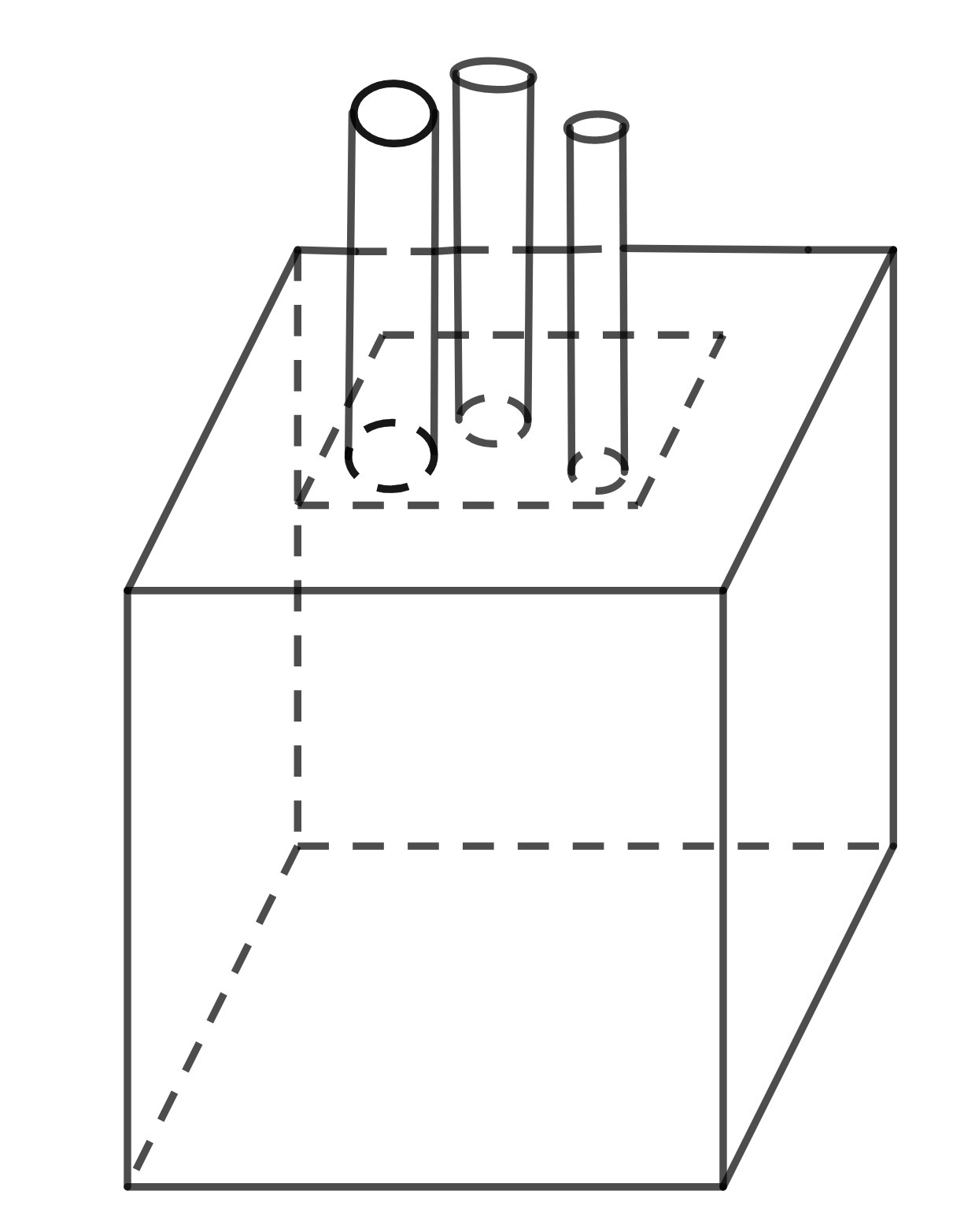
D_{\mathsf{C}}:=\left\{x=(s,\overrightarrow{\theta},x_{n})\in{{{\mathbb{R}}}^{n}};x_{n}\in\left(0,\frac{r}{2}\right),s\in\left(\frac{r}{2},r-x_{n}\right),\overrightarrow{\theta}\in[0,2\pi)^{n-2}\right\}.

The next lemma gives two cut-off functions towards the construction of the desired extension operator.

Lemma 7.2.

$(1):$ There exists a function $L^{i}_{\mathsf{C}}:\overline{A_{\mathsf{C}}}\to[0,1]$ which is continuous on $\overline{A_{\mathsf{C}}}\setminus\partial B^{n-1}(0,\frac{r}{2})\times\{0\}$ , which equals zero both on $\left(\overline{B}^{n-1}(0,r)\setminus B^{n-1}(0,\frac{r}{2})\right)\times\{0\}$ and on the set $\partial B^{n-1}(0,r)\times(0,1)$ , which equals $1$ on $\partial B^{n-1}(0,\frac{r}{2})\times(0,1)$ and which has the following additional properties. The function $L^{i}_{\mathsf{C}}$ is Lipschitz on $A_{\mathsf{C}}\setminus\overline{D_{\mathsf{C}}}$ with

|\nabla L^{i}_{\mathsf{C}}(x)|\leq\frac{C}{r}\ {\rm for}\ x\in A_{\mathsf{C}}\setminus\overline{D_{\mathsf{C}}},

and $L^{i}_{\mathsf{C}}$ is locally Lipschitz on $D_{\mathsf{C}}$ with

|\nabla L^{i}_{\mathsf{C}}(x)|\leq\frac{C}{\sqrt{(s-\frac{r}{2})^{2}+x_{n}^{2}}}\ {\rm for}\ x\in D_{\mathsf{C}}.

$(2):$ There exists a function $L^{o}_{\mathsf{C}}:\overline{A_{\mathsf{C}}}\to[0,1]$ , which is continuous on $\overline{A_{\mathsf{C}}}\setminus\partial B^{n-1}(0,\frac{r}{2})\times\{0\}$ , which equals zero on $\partial B^{n-1}(0,\frac{r}{2})\times[0,1)$ , and which equals $1$ both on $\partial B^{n-1}(0,r)\times(0,1)$ and on $\left(B^{n-1}(0,r)\setminus\overline{B}^{n-1}(0,\frac{r}{2})\right)\times\{0\},$ and which has the additional following properties. The function $L^{o}_{\mathsf{C}}$ is Lipschitz on $A_{\mathsf{C}}\setminus\overline{D_{\mathsf{C}}}$ with

|\nabla L^{o}_{\mathsf{C}}(x)|\leq\frac{C}{r}\ {\rm for}\ x\in A_{\mathsf{C}}\setminus\overline{D_{\mathsf{C}}},

and $L^{o}_{\mathsf{C}}$ is locally Lipschitz on $D_{\mathsf{C}}$ with

|\nabla L^{o}_{\mathsf{C}}(x)|\leq\frac{C}{\sqrt{(s-\frac{r}{2})^{2}+x_{n}^{2}}}\ {\rm for}\ x\in D_{\mathsf{C}}.

Proof.

$(1):$ We define the cut-off function $L^{i}_{\mathsf{C}}$ on $\overline{A_{\mathsf{C}}}$ with respect to the cylindrical coordinate system $\{x=(s,\overrightarrow{\theta},x_{n})\in{{{\mathbb{R}}}^{n}}\}$ by setting

(7.2)

L^{i}_{\mathsf{C}}(x)=\begin{cases}\frac{-2}{r}s+2,&x\in\overline{A_{\mathsf{C}}}\setminus\overline{D_{\mathsf{C}}},\\ \frac{x_{n}}{x_{n}+(s-\frac{r}{2})},&x\in\overline{D_{\mathsf{C}}}\setminus\partial B^{n-1}(0,\frac{r}{2})\times\{0\},\\ 0,&x\in\partial B^{n-1}(0,\frac{r}{2})\times\{0\}\,.\end{cases}

Then, if $x\in A_{\mathsf{C}}\setminus\overline{D_{\mathsf{C}}}$ , we have

\frac{\partial L^{i}_{\mathsf{C}}(x)}{\partial\theta_{1}}=...=\frac{\partial L^{i}_{\mathsf{C}}(x)}{\partial\theta_{n-2}}=\frac{\partial L^{i}_{\mathsf{C}}(x)}{\partial x_{n}}=0\,\,\text{and}\,\,\left|\frac{\partial L^{i}_{\mathsf{C}}(x)}{\partial s}\right|=\frac{2}{r}.

If $x\in{D_{\mathsf{C}}},$ we have

\frac{\partial L^{i}_{\mathsf{C}}(x)}{\partial\theta_{1}}=...=\frac{\partial L^{i}_{\mathsf{C}}(x)}{\partial\theta_{n-2}}=0,

\left|\frac{\partial L^{i}_{\mathsf{C}}(x)}{\partial s}\right|=\left|\frac{x_{n}}{\left(x_{n}+(s-\frac{r}{2})\right)^{2}}\right|\leq\left|\frac{x_{n}+(s-\frac{r}{2})}{\left(x_{n}+(s-\frac{r}{2})\right)^{2}}\right|\leq\frac{1}{\sqrt{(s-\frac{r}{2})^{2}+x_{n}^{2}}}

and

\left|\frac{\partial L^{i}_{\mathsf{C}}(x)}{\partial x_{n}}\right|=\left|\frac{(s-\frac{r}{2})}{\left(x_{n}+(s-\frac{r}{2})\right)^{2}}\right|\leq\left|\frac{x_{n}+(s-\frac{r}{2})}{\left(x_{n}+(s-\frac{r}{2})\right)^{2}}\right|\leq\frac{1}{\sqrt{(s-\frac{r}{2})^{2}+x_{n}^{2}}}.

Hence, we obtain

(7.3)

|\nabla L^{i}_{\mathsf{C}}(x)|\leq\begin{cases}\frac{C}{r},&x\in A_{\mathsf{C}}\setminus\overline{D_{\mathsf{C}}},\\ \frac{C}{\sqrt{(s-\frac{r}{2})^{2}+x_{n}^{2}}},&x\in{D_{\mathsf{C}}}.\end{cases}

$(2):$ We define the cut-off function $L^{o}_{\mathsf{C}}$ on $\overline{A_{\mathsf{C}}}$ with respect to the cylindrical coordinate system $\{x=(s,\overrightarrow{\theta},x_{n})\in{{{\mathbb{R}}}^{n}}\}$ by setting

(7.4)

L^{o}_{\mathsf{C}}(x)=\begin{cases}\frac{2}{r}s-1,&x\in\overline{A_{\mathsf{C}}}\setminus\overline{D_{\mathsf{C}}},\\ \frac{s-\frac{r}{2}}{x_{n}+(s-\frac{r}{2})},&x\in\overline{D_{\mathsf{C}}}\setminus\partial B^{n-1}(0,\frac{r}{2})\times\{0\},\\ 0,&x\in\partial B^{n-1}(0,\frac{r}{2})\times\{0\}\,.\end{cases}

By similar computations, we have

(7.5)

|\nabla L^{o}_{\mathsf{C}}(x)|\leq\begin{cases}\frac{C}{r},&x\in A_{\mathsf{C}}\setminus\overline{D_{\mathsf{C}}},\\ \frac{C}{\sqrt{x_{n}^{2}+(s-\frac{r}{2})^{2}}},&x\in{D_{\mathsf{C}}}.\end{cases}

∎

7.3. The extension operator

Towards the construction of our extension operator, we define piston-shaped domains $P_{k}^{j}$ by setting

P_{k}^{j}:=\mathsf{D}_{k}^{j}\times(0,1)\cup\widetilde{\mathsf{D}}_{k}^{j}\times[1,2).

The collection $\{P_{k}^{j}\}$ is pairwise disjoint. We set $U_{1}:=\mathcal{S}_{o}\times(1,2)\setminus{\Omega}_{h}.$

Given a cylinder $\mathsf{C}_{k}^{j}$ , in order to simplify our notation, we write $L^{i}_{k,j}=L^{i}_{\mathsf{C}_{k}^{j}}$ , $L^{o}_{k,j}=L^{o}_{\mathsf{C}_{k}^{j}}$ , $A_{k}^{j}=A_{\mathsf{C}_{k}^{j}}$ and $D_{k}^{j}=D_{\mathsf{C}_{k}^{j}}$ . Then we define cut-off functions $L^{i}$ and $L^{o}$ by setting

(7.6)

L^{i}(x):=\sum_{k,j}L^{i}_{k,j}(x)\ {\rm for}\ x\in\bigcup_{k,j}\overline{A_{k}^{j}},

and

(7.7)

L^{o}(x):=\sum_{k,j}L^{o}_{k,j}(x)\ \ {\rm for}\ \ x\in\bigcup_{k,j}\overline{A_{k}^{j}}.

We define a reflection on $\mathcal{S}_{o}\times(1,2)$ by setting

(7.8)

\mathcal{R}_{1}(x):=\left(x_{1},x_{2},\cdots,x_{n-1},2-x_{n}\right)\ {\rm for\ every}\ x=(x_{1},x_{2},\cdots,x_{n})\in\mathcal{S}_{o}\times(1,2).

On the set $\bigcup_{k,j}A_{k}^{j}$ , we define a mapping $\mathcal{R}_{2}$ which is a reflection on every $A_{k}^{j}$ . With respect to the local cylindrical coordinate system on every $A_{k}^{j}$ , we write

(7.9)

\mathcal{R}_{2}(x):=\mathcal{R}_{2}(s,\overrightarrow{\theta},x_{n})=\left(-\frac{s}{2}+\frac{3}{4}r_{k},\overrightarrow{\theta},x_{n}\right)

for $x=(s,\overrightarrow{\theta},x_{n})\in A_{k}^{j}$ . Simple computations give the estimates

(7.10)

\frac{1}{C}\leq|J_{\mathcal{R}_{1}}(x)|\leq C\ {\rm and}\ |D\mathcal{R}_{1}(x)|\leq C,

for every $x\in\mathcal{S}_{o}\times(1,2)$ , and

(7.11)

\frac{1}{C}\leq|J_{\mathcal{R}_{2}}(x)|\leq C\ {\rm and}\ |D\mathcal{R}_{2}(x)|\leq C,

for every $x\in\bigcup_{k,j}A_{k}^{j}$ .

We begin by defining our linear extension operator on the dense subspace $W^{1,\infty}(\widetilde{{\Omega}}_{h})\cap C(\widetilde{{\Omega}}_{h})$ of $W^{1,p}(\widetilde{{\Omega}}_{h}).$ Given $u\in W^{1,\infty}(\widetilde{{\Omega}}_{h})\cap C(\widetilde{{\Omega}}_{h})$ , we define the extension $E(u)$ on the rectangle $\mathcal{C}_{o}$ by setting

(7.12)

E(u)(x):=\begin{cases}u(x),&x\in\widetilde{{\Omega}}_{h},\\ L^{i}(x)(u\circ\mathcal{R}_{2})(x)+L^{o}(x)(u\circ\mathcal{R}_{1})(x),&x\in\bigcup_{k,j}\overline{A_{k}^{j}},\\ (u\circ\mathcal{R}_{1})(x),&x\in U_{1}\,.\end{cases}

We continue with the local properties of our extension operator.

Lemma 7.3.

Let $E$ be the extension operator defined in (7.12). Then, for every $u\in W^{1,\infty}(\widetilde{\Omega}_{h})\cap C(\widetilde{{\Omega}}_{h})$ , we have:

$(1)$ : $E(u)$ is Lipschitz on $U_{1}$ with

(7.13)

|\nabla E(u)(x)|\leq|\nabla(u\circ\mathcal{R}_{1})(x)|

for almost every $x\in U_{1}$ .

$(2)$ : $E(u)$ is locally Lipschitz on ${A_{k}^{n_{k}}}$ with

(7.14)

|\nabla E(u)(x)|\leq|\nabla L^{i}_{k,n_{k}}(x)(u\circ\mathcal{R}_{2})(x)|+|L^{i}_{k,n_{k}}(x)\nabla(u\circ\mathcal{R}_{2})(x)|\\ +|\nabla L^{o}_{k,n_{k}}(x)(u\circ\mathcal{R}_{1})(x)|+|L^{o}_{k,n_{k}}(x)\nabla(u\circ\mathcal{R}_{1})(x)|

for almost every $x\in{A_{k}^{j}}$ .

Moreover, with respect to the local cylindrical system $x=(s,\overrightarrow{\theta},x_{n})$ on $\mathsf{C}_{k}^{j}$ , for every $1\leq q<\infty$ , we have

(7.15)

\int_{\mathsf{C}_{k}^{j}}|E(u)(x)|^{q}dx\leq C\int_{P_{k}^{j}}|u(x)|^{q}dx

and

(7.16)

\int_{\mathsf{C}_{k}^{j}}|\nabla E(u)(x)|^{q}dx\leq C\int_{P_{k}^{j}}|\nabla u(x)|^{q}dx\\ +C\int_{D_{k}^{j}}\left(\sqrt{\frac{1}{x_{n}^{2}+\left(s-\frac{r_{k}}{2}\right)^{2}}}\right)^{q}(|u\circ\mathcal{R}_{1}(x)|^{q}+|u\circ\mathcal{R}_{2}(x)|^{q})dx\\ +C\int_{A_{k}^{j}\setminus\overline{D_{k}^{j}}}\left(\frac{1}{r_{k}}\right)^{q}(|u\circ\mathcal{R}_{1}(x)|^{q}+|u\circ\mathcal{R}_{2}(x)|^{q})dx,

with some uniform positive constant $C$ .

Proof.

Since $u\in W^{1,\infty}(\widetilde{\Omega}_{h})\cap C(\widetilde{{\Omega}}_{h})$ , definitions of cut-off functions $L^{i},L^{o}$ and reflections $\mathcal{R}_{1},\mathcal{R}_{2}$ easily yield that $E(u)$ is Lipschitz on $U_{1}$ and that $E(u)$ is locally Lipschitz on $A_{k}^{j}$ for every $k$ and $j$ . Inequalities (7.13) and (7.14) follow by the chain rule.

By the definition of $E(u)$ in (7.12), we have

(7.17)

\int_{\mathsf{C}_{k}^{j}}|E(u)(x)|^{q}dx\leq\int_{P_{k}^{j}}|u(x)|^{q}dx\\ +\int_{A_{k}^{j}}|L^{i}_{k,j}(x)(u\circ\mathcal{R}_{2})(x)+L^{o}_{k,j}(x)(u\circ\mathcal{R}_{1})(x)|^{q}dx.

Since $0\leq L^{i}_{k,j}(x)\leq 1$ and $0\leq L^{o}_{k,j}(x)\leq 1$ for every $x\in A_{k}^{j}$ , by (7.10), (7.11) and the change of variables formula, we have

(7.18)

\int_{A_{k}^{j}}|L^{i}_{k,j}(x)(u\circ\mathcal{R}_{2})(x)+L^{o}_{k,j}(x)(u\circ\mathcal{R}_{1})(x)|^{q}dx\\ \leq C\int_{A_{k}^{j}}|u\circ\mathcal{R}_{1}(x)|^{q}dx+C\int_{A_{k}^{j}}|u\circ\mathcal{R}_{2}(x)|^{q}dx\\ \leq C\int_{P_{k}^{j}}|u(x)|^{q}dx.

By combining inequalities (7.17) and (7.18), we obtain inequality (7.15).

By inequality (7.14), we have

(7.19)

\int_{\mathsf{C}_{k}^{j}}|\nabla E(u)(x)|^{q}dx\leq\int_{P_{k}^{j}}|\nabla u(x)|^{q}dx+I^{k,j}_{1}+I^{k,j}_{2},

where

I^{k,j}_{1}:=\int_{A_{k}^{j}}|L^{i}_{k,j}(x)\nabla(u\circ\mathcal{R}_{2})(x)|^{q}dx+\int_{A_{k}^{j}}|L^{o}_{k,j}(x)\nabla(u\circ\mathcal{R}_{1})(x)|^{q}dx

and

I^{k,j}_{2}:=\int_{A_{k}^{j}}|\nabla L^{i}_{k,j}(x)(u\circ\mathcal{R}_{2})(x)|^{q}dx+\int_{A_{k}^{j}}|\nabla L^{o}_{k,j}(x)(u\circ\mathcal{R}_{1})(x)|^{q}dx.

Arguing as for (7.18), we have

(7.20)

I^{k,j}_{1}\leq C\int_{P_{k}^{j}}|\nabla u(x)|^{q}dx.

By inequality (7.3), we have

(7.21)

\int_{A_{k}^{j}}|\nabla L^{i}_{k,j}(x)(u\circ\mathcal{R}_{2})(x)|^{q}dx\\ \leq C\int_{A_{k}^{j}\setminus\overline{D_{k}^{j}}}\left(\frac{1}{r_{k}}\right)^{q}|(u\circ\mathcal{R}_{2})(x)|^{q}dx\\ +C\int_{D_{k}^{j}}\left(\sqrt{\frac{1}{x_{n}^{2}+\left(s-\frac{r_{k}}{2}\right)^{2}}}\right)^{q}|(u\circ\mathcal{R}_{2})(x)|^{q}dx.

By (7.5), we have

(7.22)

\int_{A_{k}^{j}}|\nabla L^{o}_{k,j}(x)(u\circ\mathcal{R}_{1})(x)|^{q}dx\\ \leq C\int_{A_{k}^{j}\setminus\overline{D_{k}^{j}}}\left(\frac{1}{r_{k}}\right)^{q}|(u\circ\mathcal{R}_{1})(x)|^{q}dx\\ +C\int_{D_{k}^{j}}\left(\sqrt{\frac{1}{x_{n}^{2}+\left(s-\frac{r_{k}}{2}\right)^{2}}}\right)^{q}|(u\circ\mathcal{R}_{1})(x)|^{q}dx.

In conclusion, (7.21) and (7.22) give

(7.23)

I^{k,j}_{2}\leq C\int_{D_{k}^{j}}\left(\sqrt{\frac{1}{x_{n}^{2}+\left(s-\frac{r_{k}}{2}\right)^{2}}}\right)^{q}((|u\circ\mathcal{R}_{1})(x)|^{q}+|(u\circ\mathcal{R}_{2})(x)|^{q})dx\\ +C\int_{A_{k}^{j}\setminus\overline{D_{k}^{j}}}\left(\frac{1}{r_{k}}\right)^{q}(|(u\circ\mathcal{R}_{1})(x)|^{q}+|(u\circ\mathcal{R}_{2})(x)|^{q})dx.

Finally, by combining inequalities (7.19), (7.20) and (7.23), we obtain inequality (7.16). ∎

7.4. An extension theorem

The following theorem provides us with examples of irregular extension domains.

Theorem 7.1.

Let $1\leq q<n-1$ and ${(n-1)q}/{(n-1-q)}<p<\infty$ be fixed. Given $\lambda>0,$ define

(7.24)

h_{\lambda}(t):=\left(\frac{1}{t}\right)^{((1-\lambda(n-1-q))(n-1)(k+1)+k)/3k}.

There exists $\lambda_{o}:=\lambda_{o}(p,q)>0$ such that $\widetilde{\Omega}_{h}\subset{{{\mathbb{R}}}^{n}}$ is a Sobolev $(p,q)$ -extension domain with $|\partial\widetilde{\Omega}_{h}|>0$ whenever $h(t)\leq h_{\lambda}(t)$ for some $\lambda>\lambda_{o}$ and all $0<t\leq 1.$

Proof.

By the definition of $h_{\lambda}$ and (7.1), we have

(7.25)

r_{k}\leq 2^{-\lambda(n-1)(k+1)}.

Set

(7.26)

\lambda_{o}(p,q):=\max\left\{\frac{n-1-p}{(n-1)^{2}},\frac{p-q}{(n-1)(p-q)-pq}\right\}.

Then, for every $\lambda>\lambda_{o}$ , we have $1\leq q<\frac{((n-1)\lambda-1)p}{\lambda p+(n-1)\lambda-1}<n-1$ . Fix such a $\lambda.$ To simplify our notation, we refer to $h_{\lambda}$ by $h$ in what follows. Since $E^{n-1}\subset\partial\widetilde{\mathcal{D}}_{h}$ and $\mathcal{H}^{n-1}(E^{n-1})>0$ , we have $E^{n-1}\times[1,2]\subset\partial\widetilde{\Omega}_{h}$ and $\mathcal{H}^{n}(\partial\widetilde{\Omega}_{h})\geq\mathcal{H}^{n}(E^{n-1}\times[1,2])>0$ .

In order to prove that $E$ defined in (7.12) is a bounded extension operator, we need an approximation argument. Given $u\in W^{1,\infty}(\widetilde{\Omega}_{h})\cap C(\widetilde{\Omega}_{h})$ and $m\in\mathbb{N}$ , we define $u_{m}:=u\big|_{\widetilde{{\Omega}}_{h}^{m}}.$ Since $\widetilde{{\Omega}}_{h}^{m}$ is clearly quasiconvex, it follows that $u_{m}$ is Lipschitz and bounded. We define the extension $E^{m}(u_{m})$ of $u_{m}$ by setting

E^{m}(u_{m})(x):=\begin{cases}u_{m}(x),&x\in\widetilde{{\Omega}}^{m}_{h},\\ L^{i}(x)(u_{m}\circ\mathcal{R}_{2})(x)+L^{o}(x)(u_{m}\circ\mathcal{R}_{1})(x),&x\in\bigcup_{k=1}^{m}\bigcup_{j}\overline{A_{k}^{j}},\\ (u_{m}\circ\mathcal{R}_{1})(x),&x\in U_{1}^{m}\,,\end{cases}

where $U_{1}^{m}=\mathcal{S}_{0}\times(0,1)\setminus{\Omega}_{h}^{m}.$ Since $u_{m}$ is Lipschitz, $E^{m}(u_{m})$ is $ACL$ on $\mathcal{C}_{o}$ . By the definition of $u_{m}$ and the Hölder inequality, we have

(7.27)

\int_{\widetilde{\Omega}_{h}^{m}}|u_{m}(x)|^{q}dx\leq\int_{\widetilde{\Omega}_{h}}|u(x)|^{q}dx\leq C\left(\int_{\widetilde{\Omega}_{h}}|u(x)|^{p}dx\right)^{\frac{q}{p}}

and

(7.28)

\int_{\widetilde{\Omega}_{h}^{m}}|\nabla u_{m}(x)|^{q}dx\leq\int_{\widetilde{\Omega}_{h}}|\nabla u(x)|^{q}dx\leq C\left(\int_{\widetilde{\Omega}_{h}}|\nabla u(x)|^{p}dx\right)^{\frac{q}{p}}.

Since the collection $\{P_{k}^{j}\}$ is pairwise disjoint, by summing over $j$ and $k$ , (7.15) and the Hölder inequality imply

(7.29)

\int_{\bigcup_{k=1}^{m}\bigcup_{j}\mathsf{C}_{k}^{j}}|E^{m}(u_{m})(x)|^{q}dx\leq C\int_{\bigcup_{k=1}^{m}\bigcup_{j}P_{k}^{j}}|u_{m}(x)|^{q}dx\leq C\left(\int_{\widetilde{\Omega}_{h}}|u(x)|^{p}dx\right)^{\frac{q}{p}}.

By (7.10), the change of variables formula and the Hölder inequality, we have

(7.30)

\int_{U_{1}^{m}}|u_{m}\circ\mathcal{R}_{1}(x)|^{q}dx\leq\int_{\mathcal{R}_{1}\left(U_{1}^{m}\right)}|u_{m}(x)|^{q}dx\leq C\left(\int_{\widetilde{{\Omega}}_{h}}|u(x)|^{p}dx\right)^{\frac{q}{p}}.

Consequently, by combining (7.27), (7.29) and (7.30), we obtain

(7.31)

\left(\int_{\mathcal{C}_{o}}|E^{m}(u_{m})(x)|^{q}dx\right)^{\frac{1}{q}}\leq C\left(\int_{\widetilde{{\Omega}}_{h}}|u(x)|^{p}dx\right)^{\frac{1}{p}},

where the constant $C$ is independent of $m$ and $u$ .

By (7.13), we have

(7.32)

\int_{U_{1}^{m}}|\nabla E^{m}(u_{m})(x)|^{q}dx\leq\int_{U_{1}^{m}}|\nabla(u_{m}\circ\mathcal{R}_{1})(x)|^{q}dx.

By (7.10), the change of variables formula and the Hölder inequality, we obtain

(7.33)

\int_{U_{1}^{m}}|\nabla(u_{m}\circ\mathcal{R}_{1})(x)|^{q}dx\leq\int_{U_{1}^{m}}|\nabla(u_{m}\circ\mathcal{R}_{1})(x)|^{q}dx\\ \leq C\int_{\mathcal{R}_{1}\left(U_{1}^{m}\right)}|\nabla u_{m}(x)|^{q}dx\leq C\left(\int_{\widetilde{{\Omega}}_{h}}|\nabla u(x)|^{p}dx\right)^{\frac{q}{p}}.

By combining (7.32) and (7.33), we obtain

(7.34)

\displaystyle\int_{U_{1}^{m}}|\nabla E^{m}(u_{m})(x)|^{q}dx\leq C\left(\int_{\widetilde{{\Omega}}_{h}}|\nabla u(x)|^{p}dx\right)^{\frac{q}{p}},

where the constant $C$ is independent of $m$ and $u$ .

By (7.16) and the fact that the collection $\{P_{k}^{j}\}$ is pairwise disjoint, we have

(7.35)

\int_{\bigcup_{k=1}^{m}\bigcup_{j}\mathsf{C}_{k}^{j}}|\nabla E^{m}(u_{m})(x)|^{q}dx\leq C\int_{\bigcup_{k=1}^{m}\bigcup_{j}P_{k}^{j}}|\nabla u_{m}(x)|^{q}dx\\ +C\int_{\bigcup_{k=1}^{m}\bigcup_{j}D_{k}^{j}}\left(\sqrt{\frac{1}{x_{n}^{2}+\left(s-\frac{r_{k}}{2}\right)^{2}}}\right)^{q}(|(u_{m}\circ\mathcal{R}_{1})(x)|^{q}+|(u_{m}\circ\mathcal{R}_{2})(x)|^{q})dx\\ +C\int_{\bigcup_{k=1}^{m}\bigcup_{j}A_{k}^{j}\setminus\overline{D_{k}^{j}}}\left(\frac{1}{r_{k}}\right)^{q}(|(u_{m}\circ\mathcal{R}_{1})(x)|^{q}+|(u_{m}\circ\mathcal{R}_{2})(x)|^{q})dx.

The Hölder inequality gives

(7.36)

\int_{\bigcup_{k=1}^{m}\bigcup_{j}P_{k}^{j}}|\nabla u_{m}(x)|^{q}dx\leq C\left(\int_{\widetilde{\Omega}_{h}}|\nabla u(x)|^{p}dx\right)^{\frac{q}{p}},

(7.37)

\int_{\bigcup_{k=1}^{m}\bigcup_{j}D_{k}^{j}}\left(\sqrt{\frac{1}{x_{n}^{2}+\left(s-\frac{r_{k}}{2}\right)^{2}}}\right)^{q}(|(u_{m}\circ\mathcal{R}_{1})(x)|^{q}+|(u_{m}\circ\mathcal{R}_{2})(x)|^{q})dx\\ \leq C\left(\int_{\bigcup_{k=1}^{m}\bigcup_{j}D_{k}^{j}}|(u_{m}\circ\mathcal{R}_{1})(x)|^{p}+|(u_{m}\circ\mathcal{R}_{2})(x)|^{p}dx\right)^{\frac{q}{p}}\\ \times\left(\int_{\bigcup_{k=1}^{m}\bigcup_{j}D_{k}^{j}}\left(\sqrt{\frac{1}{x_{n}^{2}+\left(s-\frac{r_{k}}{2}\right)^{2}}}\right)^{\frac{pq}{p-q}}dx\right)^{\frac{p-q}{p}}

and

(7.38)

\int_{\bigcup_{k=1}^{m}\bigcup_{j}A_{k}^{j}\setminus\overline{D_{k}^{j}}}\left(\frac{1}{r_{k}}\right)^{q}(|(u_{m}\circ\mathcal{R}_{1})(x)|^{q}+|(u_{m}\circ\mathcal{R}_{2})(x)|^{q})dx\\ \leq\left(\int_{\bigcup_{k=1}^{m}\bigcup_{j}A_{k}^{j}\setminus\overline{D_{k}^{j}}}|(u_{m}\circ\mathcal{R}_{1})(x)|^{p}+|(u_{m}\circ\mathcal{R}_{2})(x)|^{p}dx\right)^{\frac{q}{p}}\\ \times\left(\int_{\bigcup_{k=1}^{m}\bigcup_{j}A_{k}^{j}\setminus\overline{D_{k}^{j}}}\left(\frac{1}{r_{k}}\right)^{\frac{pq}{p-q}}dx\right)^{\frac{p-q}{p}}.

By (7.10) and (7.11), the change of variables formula yields that

(7.39)

\int_{\bigcup_{k=1}^{m}\bigcup_{j}A_{k}^{j}\setminus\overline{D_{k}^{j}}}|(u_{m}\circ\mathcal{R}_{1})(x)|^{p}+|(u_{m}\circ\mathcal{R}_{2})(x)|^{p}dx\leq C\int_{\widetilde{\Omega}_{h}}|u(x)|^{p}dx

and

(7.40)

\int_{\bigcup_{k=1}^{m}\bigcup_{j}D_{k}^{j}}|(u_{m}\circ\mathcal{R}_{1})(x)|^{p}+|(u_{m}\circ\mathcal{R}_{2})(x)|^{p}dx\leq C\int_{\widetilde{\Omega}_{h}}|u(x)|^{p}dx.

With $l_{k}=\sqrt{x_{n}^{2}+\left(s-\frac{r_{k}}{2}\right)^{2}}$ , by (7.25) and (7.26), we have

(7.41)

\int_{\bigcup_{k=1}^{m}\bigcup_{j}D_{k}^{j}}\left(\frac{1}{\sqrt{x_{n}^{2}+\left(s-\frac{r_{k}}{2}\right)^{2}}}\right)^{\frac{pq}{p-q}}dx\leq C\sum_{k=1}^{m}\sum_{j}r_{k}\int_{0}^{r_{k}}l_{k}^{n-2-\frac{pq}{p-q}}dl_{k}\\ \leq C\sum_{k=1}^{m}\sum_{j}r_{k}^{n-\frac{pq}{p-q}}\leq C\sum_{k=1}^{\infty}2^{(n-1)(k+1)\left(1-\lambda\left(n-\frac{pq}{p-q}\right)\right)}<\infty.

Furthermore,

(7.42)

\int_{\bigcup_{k=1}^{m}\bigcup_{j}A_{k}^{j}\setminus\overline{D_{k}^{j}}}\left(\frac{1}{r_{k}}\right)^{\frac{pq}{p-q}}dx\leq C\sum_{k=1}^{m}\sum_{j=1}^{N_{k}}r_{k}^{n-1-\frac{pq}{p-q}}\\ \leq C\sum_{k=1}^{\infty}2^{(n-1)(k+1)\left(1-\lambda\left(n-1-\frac{pq}{p-q}\right)\right)}<\infty.

By combining inequalities (7.35)-(7.42), we deduce that

(7.43)

\int_{\bigcup_{k=1}^{m}\bigcup_{j}\mathsf{C}_{k}^{j}}|\nabla E^{m}(u_{m})(x)|^{q}dx\leq C\left(\int_{\widetilde{\Omega}_{h}}|u(x)|^{p}+|\nabla u(x)|^{p}dx\right)^{\frac{q}{p}}.

Next, by combining (7.28), (7.34) and (7.43), we conclude that

(7.44)

\int_{\mathcal{C}_{o}}|\nabla E^{m}(u_{m})(x)|^{q}dx\leq C\left(\int_{\widetilde{\Omega}_{h}}|u(x)|^{p}+|\nabla u(x)|^{p}dx\right)^{\frac{q}{p}}.

Hence, by combining (7.31) and (7.44), we infer that

(7.45)

\|E^{m}(u_{m})\|_{W^{1,q}(\mathcal{C}_{o})}\leq C\|u\|_{W^{1,p}(\widetilde{{\Omega}}_{h})},

uniformly in $m$ .

By the definitions of $u_{m}$ and $E^{m}(u_{m})$ , for arbitrary $m,m^{\prime}\in\mathbb{N}$ with $m<m^{\prime}$ , we have

(7.46)

\|E^{m}(u_{m})-E^{m^{\prime}}(u_{m^{\prime}})\|^{q}_{W^{1,q}(\mathcal{C}_{o})}\leq\int_{\bigcup_{k=m+1}^{m^{\prime}}\bigcup_{j}\mathsf{C}_{k}^{j}}\left(|E^{m}(u_{m})(x)|^{q}+|\nabla E^{m}(u_{m})(x)|^{q}\right)dx\\ +\int_{\bigcup_{k=m+1}^{m^{\prime}}\bigcup_{j}\mathsf{C}_{k}^{j}}\left(|E^{m^{\prime}}(u_{m^{\prime}})(x)|^{q}+|\nabla E^{m^{\prime}}(u_{m^{\prime}})(x)|^{q}\right)dx.

By the definition of $E^{m}(u_{m})$ and $E^{m^{\prime}}(u_{m^{\prime}})$ , the Hölder inequality implies

(7.47)

\int_{\bigcup_{k=m+1}^{m^{\prime}}\bigcup_{j}\mathsf{C}_{k}^{j}}\left(|E^{m}(u_{m})(x)|^{q}+|\nabla E^{m}(u_{m})(x)|^{q}\right)dx\\ \leq C\int_{\mathcal{R}_{1}\left(\bigcup_{k=m+1}^{m^{\prime}}\bigcup_{j}\mathsf{C}_{k}^{j}\right)}\left(|u_{m}(x)|^{q}+|\nabla u_{m}(x)|^{q}\right)dx\\ \leq C(p,q)\left(\int_{\mathcal{R}_{1}\left(\bigcup_{k=m+1}^{m^{\prime}}\bigcup_{j}\mathsf{C}_{k}^{j}\right)}\left(|u(x)|^{p}+|\nabla u(x)|^{p}\right)dx\right)^{\frac{q}{p}},

and

(7.48)

\int_{\bigcup_{k=m+1}^{m^{\prime}}\bigcup_{j}\mathsf{C}_{k}^{j}}\left(|E^{m^{\prime}}(u_{m^{\prime}})(x)|^{q}+|\nabla E^{m^{\prime}}(u_{m^{\prime}})(x)|^{q}\right)dx\leq\\ C\left(\int_{\bigcup_{k=m+1}^{m^{\prime}}\bigcup_{j}\widetilde{\mathsf{C}}_{k}^{j}}\left(|u_{m^{\prime}}|^{p}+|\nabla u_{m^{\prime}}|^{p}\right)dx+\int_{\mathcal{R}_{1}\left(\bigcup_{k=m+1}^{m^{\prime}}\bigcup_{j}A_{k}^{j}\right)}\left(|u_{m^{\prime}}|^{p}+|\nabla u_{m^{\prime}}|^{p}\right)dx\right)^{\frac{q}{p}}\\ \leq C\left(\int_{\bigcup_{k=m+1}^{m^{\prime}}\bigcup_{j}\widetilde{\mathsf{C}}_{k}^{j}}\left(|u|^{p}+|\nabla u|^{p}\right)dx+\int_{\mathcal{R}_{1}\left(\bigcup_{k=m+1}^{m^{\prime}}\bigcup_{j}A_{k}^{j}\right)}\left(|u|^{p}+|\nabla u|^{p}\right)dx\right)^{\frac{q}{p}}.

Since the volumes of $\mathcal{R}_{1}\left(\bigcup_{k=m+1}^{m^{\prime}}\bigcup_{j}A_{k}^{j}\right)$ and of $\bigcup_{k=m+1}^{m^{\prime}}\bigcup_{j}\widetilde{\mathsf{C}}_{k}^{j}$ tend to zero as $m,m^{\prime}$ approach infinity, both terms in (7.47) and (7.48) converge to zero. Consequently, $\{E^{m}(u_{m})\}$ is a Cauchy sequence in the Sobolev space $W^{1,q}(\mathcal{C}_{o})$ and hence converges to some function $v\in W^{1,q}(\mathcal{C}_{o})$ with respect to the $W^{1,q}$ -norm. Furthermore, there exists a subsequence of $\{E^{m}(u_{m})\}$ which converges to $v$ almost everywhere in $\mathcal{C}_{o}$ . On the other hand, by the definitions of $E^{m}(u_{m})$ and $E(u)$ , we have

\lim_{m\to\infty}E^{m}(u_{m})(x)=E(u)(x)

for almost every $x\in\mathcal{C}_{o}$ . Hence $v(x)=E(u)(x)$ almost everywhere. This implies that $E(u)\in W^{1,q}(\mathcal{C}_{o})$ with

(7.49)

\|E(u)\|_{W^{1,q}(\mathcal{C}_{o})}=\|v\|_{W^{1,q}(\mathcal{C}_{o})}=\lim_{m\to\infty}\|E^{m}(u_{m})\|_{W^{1,q}(\mathcal{C}_{o})}\leq C\|u\|_{W^{1,p}(\widetilde{{\Omega}}_{h})}.

We conclude that $E$ defined in (7.12) is a linear extension operator from $W^{1,\infty}(\widetilde{{\Omega}}_{h})\cap C(\widetilde{{\Omega}}_{h})$ to $W^{1,q}(\mathcal{C}_{o})$ with the norm inequality

\|E(u)\|_{W^{1,q}(\mathcal{C}_{o})}\leq C\|u\|_{W^{1,p}(\widetilde{\Omega}_{h})},

where $C$ is independent of $u$ . Since $W^{1,\infty}(\widetilde{{\Omega}}_{h})\cap C(\widetilde{{\Omega}}_{h})$ is dense in $W^{1,p}(\widetilde{{\Omega}}_{h})$ , we can extend $E$ to entire $W^{1,p}(\widetilde{{\Omega}}_{h})$ . It follows that $\widetilde{\Omega}_{h}$ is a Sobolev $(p,q)$ -extension domain, since $\mathcal{C}_{o}$ is a $(q,q)$ -extension domain. ∎

7.5. Proofs of Theorem 1.7 and 1.8

Proof of Theorem 1.7.

The claim is an immediate consequence of Theorem 7.1. ∎

Proof of Theorem 1.8.

Let $n\geq 3$ and $1\leq q<n-1$ . Fix $(n-1)q/(n-1-q)<p<\infty$ and a strictly increasing and continuous function $h:[0,1]\to[0,1]$ . Fix $\lambda>\lambda_{o},$ where $\lambda_{o}$ is from Theorem 7.1. Define

\tilde{h}(t):=\min\left\{h(t),\left(\frac{1}{t}\right)^{((1-\lambda(n-1-q))(n-1)(k+1)+k)/3k}\right\}.

Then $\widetilde{{\Omega}_{\tilde{h}}}$ is a Sobolev $(p,q)$ -extension domain by Theorem 7.1. Let $A:=E^{n-1}\times\left(\frac{3}{2},2\right)$ . Then $A\subset\partial\widetilde{{\Omega}_{\tilde{h}}}$ and $|A|>0$ . Let $0<r<\frac{1}{4}$ and $x\in A$ be arbitrary.

We define a cut-off function on the ball $B(x,r)$ by setting

(7.50)

F_{h}(y)=\begin{cases}1&\textnormal{in }B(x,\frac{r}{4}),\\ \frac{-4}{r}|y-x|+2&\textnormal{in }B(x,\frac{r}{2})\setminus B(x,\frac{r}{4}),\\ 0&\textnormal{in }B(x,r)\setminus B(x,\frac{r}{2})\,.\end{cases}

Set $u(y)=\chi_{\widetilde{{\Omega}_{\tilde{h}}}}(y)$ . Since $\widetilde{{\Omega}_{\tilde{h}}}$ is a Sobolev $(p,q)$ -extension domain, $E(u)\in W^{1,q}(\mathcal{C}_{o})$ . The function $v$ defined by $v(y):=F_{h}(y)E(u)(y)$ for $y\in B(x,r)$ satisfies

v\in\mathcal{W}_{q}\left(\widetilde{{\Omega}_{\tilde{h}}}\cap B\left(x,\frac{r}{4}\right),\widetilde{{\Omega}_{\tilde{h}}}\cap A\left(x;\frac{r}{2},\frac{3r}{4}\right);B(x,r)\right).

Pick $k_{r}\in\mathbb{N}$ so that $2^{-k_{r}-2}<r\leq 2^{-k_{r}-1}.$ If $\mathsf{C}_{k}^{j}\cap B(x,r)\neq\emptyset,$ then, by the definition of $\mathsf{C}_{k}^{j},$ we have that $k>k_{r}.$ Moreover, by the definition of $E(u)$ in (7.12), we have that

|\nabla v(y)|\leq\begin{cases}\frac{C}{r_{k}},&\ {\rm for\ every}\ y\in\mathsf{C}_{k}^{j}\cap B(x,r),\\ 0,&\ {\rm elsewhere}\,.\end{cases}

Hence, by the definition of $v$ , we have

(7.51)

\int_{B(x,r)}|\nabla v(y)|^{q}dy\leq\sum_{k=k_{r}}^{\infty}\sum_{j}\int_{\mathsf{C}_{k}^{j}\cap B(x,r)}|\nabla v(y)|^{q}dy\\ \leq C\sum_{k=k_{r}}^{\infty}r2^{(n-1)(k+1)}r_{k}^{n-1-q}\leq C\sum_{k=k_{r}}^{\infty}r2^{-k}\tilde{h}(8^{-k})\leq Crh(r).

Thus

Cap_{q}\left(\widetilde{{\Omega}_{\tilde{h}}}\cap B\left(x,\frac{r}{4}\right),\widetilde{{\Omega}_{\tilde{h}}}\cap A\left(x;\frac{r}{2},\frac{3r}{4}\right);B(x,r)\right)\leq Crh(r).

This implies that

\limsup_{r\to 0^{+}}\frac{Cap_{q}\left(\widetilde{{\Omega}_{\tilde{h}}}\cap B\left(x,\frac{r}{4}\right),\widetilde{{\Omega}_{\tilde{h}}}\cap A\left(x;\frac{r}{2},\frac{3r}{4}\right);B(x,r)\right)}{h(r)}\leq\lim_{r\to 0^{+}}Cr=0,

as desired. ∎

Remark 7.1.

One can easily modify the construction of the domain from the previous proof so as to obtain a domain that fails to be $(n-1)$ -fat at points of positive volume of the boundary. Let us sketch the necessary changes since we cannot use an extension operator as in the previous argument.

First, define $r_{k}=2^{-k-2}\exp(-\exp(2^{k}))$ and $R_{k}=2^{-k-2}.$ Instead of $E(u)$ in the above computation, we use a function $u$ defined as follows. On each $Q_{k}^{j}\times[1,2),$ our function $u$ as a function of $(y^{\prime},t)$ satisfies $u(y^{\prime},t)=1$ if $y\in\mathsf{D}_{k}^{j},$ $u(y^{\prime},t)=0$ if $y^{\prime}\notin B^{n-1}(x_{k}^{j},R_{k})$ and $u(y^{\prime},t)=\frac{\log(\frac{R_{k}}{|y^{\prime}-x_{k}^{j}|})}{\log(\frac{R_{k}}{r_{k}})}$ otherwise. Define $v(y)=F_{h}(y)u(y).$ Then a simple computation gives what we want.

8. Final comments

In this section, we discuss in more detail some of the issues mentioned in the introduction and pose open problems that are motivated by the results in this paper.

First of all, let us comment on the locality of the estimate (1.6) from Theorem 1.3 that holds for almost every $x$ for $0<r<r_{x}.$ When $q>n-1,$ we actually have this estimate for all $x$ and all $0<r<\min\{1,{\mathop{\mathrm{}}{\,diam\,}}(\Omega)/4\}.$ This also holds when $q=1$ and $n=2.$

Corollary 8.1.

Suppose that $1\leq q<p$ when $n=2$ or that $n-1<q<p$ when $n\geq 3.$ If ${\Omega}$ is a Sobolev $(p,q)$ -extension domain, then there is a nonnegative, bounded and countably additive set function $\Phi$ defined on open sets, with the following property. For each $x\in\partial{\Omega}$ and every $0<r<\min\{1,\frac{1}{4}{\mathop{\mathrm{}}{\,diam\,}}({\Omega})\},$ we have

(8.1)

\Phi(B(x,r))^{p-q}|B(x,r)\cap{\Omega}|^{q}\geq|B(x,r)|^{q}.

This conclusion follows by combining Theorem 1.1 with Remark 3.1, see inequality (3.2). Moreover, Theorem 1.1 shows that (8.1) holds also uniformly in $x$ and $r$ for $1\leq q\leq n-1$ if we assume that (3.2) holds for these values.

One can view the uniform validity of (8.1) as the optimal analog of the Ahlfors-regularity condition (1.1). In [9, 10], it was shown, relying on (1.1), that a Sobolev $(p,p)$ -extension domain can be equipped with a linear extension operator. We proved in Lemma 2.1 that a Sobolev $(p,q)$ -extension domain can be equipped with a homogeneous extension operator but we do not know if one could promote this to linearity. This motivates the following problem.

Question 8.1.

Suppose that $\Omega$ is a bounded domain that satisfies the conclusion of Corollary 8.1. Find the additional assumptions that ensure the existence of a linear extension operator from $W^{1,p}(\Omega)$ to $W^{1,q}({{{\mathbb{R}}}^{n}}).$

Given $1\leq q<n-1,$ we constructed a Sobolev $(p,q)$ -extension domain whose boundary has positive volume. We do not know if such domains exist also when $q=n-1>1.$

Question 8.2.

Let $n\geq 3.$ Does there exist a Sobolev $(p,n-1)$ -extension domain ${\Omega}\subset{{{\mathbb{R}}}^{n}},$ for some $p>n-1,$ so that $|\partial{\Omega}|>0$ ?

Furthermore, our constructions of examples of $(p,q)$ -extension domains with positive boundary volume have restrictions on $p$ in terms of $q.$ Even though these restrictions are natural for our constructions, we do not know if some other constructions would allow $p$ to be arbitrarily close to $q.$

Question 8.3.

Given $n\geq 3,$ $1\leq q<n-1$ and $p>q,$ does there exist a Sobolev $(p,q)$ -extension domain $\Omega\subset{{{\mathbb{R}}}^{n}}$ whose boundary has positive volume?

Finally, the reader familiar with [9] may wonder why we do not employ the argument that was used there to prove (1.1) towards establishing (8.1) in the case $q<n.$ We have indeed tried this but without success.

References

[1] M. Bonk, J. Heinonen and P. Koskela, Uniformizing Gromov hyperbolic spaces. Astérisque No. 270 (2001), viii+99 pp.
[2] A. P. Calderón, Lebesgue spaces of differentiable functions and distributions, Proc. Symp. Pure Math. 4 (1961), 33–49.
[3] L. C. Evans and R. F. Grariepy, Measure theory and fine properties of functions. Revised edition. Textbooks in Mathematics. CRC Press, Boca Raton, FL, 2015.
[4] B. Fuglede, Quasi topology and fine topology. Séminaire Brelot-Choquet-Deny. Théorie du potentiel, tome 10, no.2 (1965-1966), exp. no.12, p. 1–14.
[5] F. W. Gehring and B. G. Osgood, Uniform domains and the quasihyperbolic metric. J. Analyse Math. 36 (1979), 50–74 (1980).
[6] D. Gilbarg and N. S. Trudinger, Elliptic partial differential equations of second order. Reprint of the 1998 edition. Classics in Mathematics. Springer-Verlag, Berlin, 2001.
[7] V. M. Gol’dshtein, Yu. G. Reshetnyak, Quasiconformal mappings and Sobolev spaces. Dordrecht, Boston, London: Kluwer Academic Publishers, 1990.
[8] V. M. Gol’dshtein and V. N. Sitnikov, Continuation of functions of the class $W^{1}_{p}$ across Hölder boundaries. (Russian) Imbedding theorems and their applications, 31–43, Trudy Sem. S. L. Soboleva, No. 1, 1982, Akad. Nauk SSSR Sibirsk. Otdel., Inst. Mat., Novosibirsk, 1982.
[9] P. Haȷlasz, P. Koskela and H. Tuominen, Sobolev embeddings, extensions and measure density condition. J. Funct. Anal. 254 (2008), 1217-1234.
[10] P. Hajłasz, P. Koskela and H. Tuominen, Measure density and extendability of Sobolev functions. Rev. Mat. Iberoam. 24 (2008), no. 2, 645–669.
[11] J. Heinonen, The boundary absolute continuity of quasiconformal mappings II. Rev. Mat. Iberoamericana 12 (1996), no. 3, 697–725.
[12] J. Heinonen, T. Kilpeläinen and O. Martio, Nonlinear potential theory of degenerate elliptic equations. Oxford Mathematical Monographs. Oxford Science Publications. The Clarendon Press, Oxford University Press, New York, 1993.
[13] J. Heinonen and P. Koskela, Quasiconformal maps in metric spaces with controlled geometry. Acta Math. 181 (1998), no. 1, 1–61.
[14] S. Hencl and P. Koskela, Lectures on mappings of finite distortion. Lecture Notes on Mathematics 2096, Springer.
[15] P. W. Jones, Quasiconformal mappings and extendability of functions in Sobolev spaces. Acta Math. 147 (1981) 71–78.
[16] T. Kilpeläinen, A remark on the uniqueness of quasi continuous functions. Ann. Acad. Sci. Fenn. Math. 23 (1998), no. 1, 261–262.
[17] P. Koskela, Extensions and imbeddings. J. Funct. Anal. 159 (1998), no. 2, 369–383.
[18] P. Koskela, T. Rajala and Y. Zhang, A density problem for Sobolev spaces on Gromov hyperbolic domains. Nonlinear Anal. 154 (2017), 189–209.
[19] P. Koskela, T. Rajala and Y. Zhang, A geometric characterization of planar Sobolev extension domains. https://arxiv.org/abs/1502.04139.
[20] P. Koskela, T. Rajala and Y. Zhang, Planar $W^{1,1}$ -extension domains. contained in JYU-dissertation.
[21] P.Koskela and S. Rohde, Hausdorff dimension and mean porosity, Math. Ann. 309 (1997), no. 4, 593–609.
[22] P. Koskela and Z. Zhu, Product of extension domains is still an extension domain. Indiana Univ. Math. J. 69 (2020), no. 1, 137–150.
[23] P. Lahti, A notion of fine continuity for BV functions on metric spaces. Potential Anal. 46 (2017), no. 2, 279–294.
[24] D. Lučić, T. Rajala and J. Takanen, Dimension extimates for the boundary of planar Sobolev extension domains, https://arxiv.org/abs/2006.14213.
[25] V. Maz’ya, Sobolev spaces: with applications to elliptic partial differential equations. Springer, Berlin/Heidelberg, 2010.
[26] V. G. Maz’ya and S. V. Poborchi, On extension of functions in Sobolev classes to the exterior of a domain with the vertex of a peak on the boundary, Dokl. Akad. Nauk SSSR 275:5 (1984) 1066–1069 (Russian). English translation: Soviet Math. 29 (1984) 361–364.
[27] V. G. Maz’ya and S. V. Poborchi, Extension of functions in Sobolev classes to the exterior of a domain with the vertex of a peak on the boundary I, Czech. Math. Journ. 36:111 (1986) 634–661 (Russian).
[28] V. G. Maz’ya and S. V. Poborchi, Differentiable functions on bad domains, World Scientific Publishing Co., River Edge, NJ, 1997.
[29] V. G. Maz’ya and S. V. Poborchi, Extension of functions in Sobolev classes to the exterior of a domain with the vertex of a peak on the boundary II, Czech. Math. Journ. 37:112 (1987) 128–150 (Russian).
[30] P. Shvartsman, On Sobolev extension domains in ${{{\mathbb{R}}}^{n}}$ . J. Funct. Anal. 258 (2010), no. 7, 2205–2245.
[31] P. Shvartsman, N. Zobin, On planar Sobolev $L^{m}_{p}$ -extension domains. Adv. Math., 287 (2016), 237–346.
[32] H. J. S. Smith, On the integration of discontinuous functions. Proc. of the London Mathematical Society. 1874. First series. 6: 140–153.
[33] E. M. Stein, Singular integrals and differentiability properties of functions. Princeton University Press, Princeton, 1971.
[34] E. M. Stein, Harmonic analysis: real-variable methods, orthogonality, and oscillatory integrals. With the assistance of Timothy S. Murphy. Princeton Mathematical Series, 43. Monographs in Harmonic Analysis, III. Princeton University Press, Princeton, NJ, 1993.
[35] T. Rado, P. V. Reichelderfer, Continuous transformations in analysis. Berlin: Springer-Verlag, 1955.
[36] A. D. Ukhlov, Lower estimates for the norm of the extension operator of the weak differentiable functions on domains of Carnot groups. Proc. of the Khabarovsk State Univ. Mathematics, 8 (1999), 33–44.
[37] A. D. Ukhlov, Extension operators on Sobolev spaces with decreasing integrability. Trans. Razmadze Math. Inst., 174 (2020), 381–388.
[38] J. Väisälä, Quasiconformal maps and positive boundary measure. Analysis 9 (1989), no. 1-2, 205–216.
[39] J. Väisälä, The free quasiworld. Freely quasiconformal and related maps in Banach spaces. Quasiconformal geometry and dynamics (Lublin, 1996), 55–118, Banach Center Publ., 48, Polish Acad. Sci. Inst. Math., Warsaw, 1999.
[40] S. K. Vodop’yanov, V. M. Gol’dstein, T. G. Latfullin, A criterion for the extension of functions of the class $L^{1}_{2}$ from unbounded plane domains. Siberian. Math. J., 20 (1979), 416–419.
[41] S. K. Vodop’yanov and A. D. Ukhlov, Set functions and their applications in the theory of Lebesgue and Sobolev spaces. I [Translation of Mat. Tr. 6 (2003), no. 2, 14–65; MR2033646]. Siberian Adv. Math. 14 (2004), no. 4, 78–125 (2005).
[42] S. K. Vodop’yanov and A. D. Ukhlov, Set functions and their applications in the theory of Lebesgue and Sobolev spaces. II [Translation of Mat. Tr. 7 (2004), no. 1, 13–49; MR2068275]. Siberian Adv. Math. 15 (2005), no. 1, 91–125.
[43] Z. Zhu, Sobolev Functions and Mappings on Cuspidal Domains, JYU-Dissertation no. 253 (2020).
[44] W. P. Ziemer, Weakly differentiable functions. Sobolev spaces and functions of bounded variation. Graduate Texts in Mathematics, 120. Springer-Verlag, New York, 1989.

The volume of the boundary of a Sobolev (p,q)(p,q)-extension domainThanks: The first and third authors have been supported by the Academy of Finland (project No. 323960). The third author thanks Tero Kilpeläinen for introducing him to fine topology.

Abstract.

2010 Mathematics Subject Classification

1. Introduction

Theorem 1.1.

Theorem 1.2.

Corollary 1.1.

Proposition 1.1.

Theorem 1.3.

Theorem 1.4.

Theorem 1.5.

Theorem 1.6.

Theorem 1.7.

Theorem 1.8.

2. Preliminaries

2.1. Definitions and notation

Definition 2.1.

Definition 2.2.

Lemma 2.1.

Proof.

Definition 2.3.

2.2. Fine Topology

Definition 2.4.

Lemma 2.2.

Definition 2.5.

Lemma 2.3.

Definition 2.6.

Definition 2.7.

Definition 2.8.

Lemma 2.4.

Lemma 2.5.

Lemma 2.6.

Proof.

2.3. A set function associated with the extension operator

Theorem 2.1.

Proof.

Corollary 2.1.

Lemma 2.7.

2.4. Gromov hyperbolicity

Definition 2.9.

Definition 2.10.

Definition 2.11.

Lemma 2.8.

Lemma 2.9.

3. Proof of Theorem 1.4

Theorem 3.1.

Proof.

Remark 3.1.

4. Proofs of Corollary 1.1 and Theorems 1.1, 1.3, 1.5 and 1.6

Proof of Theorem 1.1.

Proof of Theorem 1.3.

Proof of Theorem 1.5.

Proof of Theorem 1.6.

Proof of Corollary 1.1.

5. Proof of Theorem 1.2

Proof of Theorem 1.2.

Lemma 5.1.

Proof.

Sharpness of (1.3).

6. Proof of Proposition 1.1

Proof of Proposition 1.1.

7. Proofs of Theorem 1.7 and Theorem 1.8

7.1. The initial construction

Lemma 7.1.

7.2. Cut-off functions

Lemma 7.2.

Proof.

7.3. The extension operator

Lemma 7.3.

Proof.

7.4. An extension theorem

Theorem 7.1.

Proof.

7.5. Proofs of Theorem 1.7 and 1.8

Proof of Theorem 1.7.

Proof of Theorem 1.8.

Remark 7.1.

8. Final comments

Corollary 8.1.

Question 8.1.

The volume of the boundary of a Sobolev $(p,q)$ -extension domainThanks: The first and third authors have been supported by the Academy of Finland (project No. 323960). The third author thanks Tero Kilpeläinen for introducing him to fine topology.