Twisted superfluid and supersolid phases of triplons in bilayer honeycomb magnets

The observation of twisted, multi-orbital superfluid in binary mixtures of ultracold ⁸⁷Rb atoms in two different hyperfine states on a honeycomb optical lattice has attracted heightened interest in this novel quantum state of matter Soltan-Panahi et al. 2011. The twisted superfluid (or twisted supersolid) state is characterised by a complex order parameter – the phase of the local superfluid order parameter at each site changes continuously forming a“twisting pattern”, thus breaking time reversal symmetry spontaneously. Interestingly, complex order parameters have experimentally been shown to be associated with other novel strongly correlated phases such as the superconducting states of $\text{Sr}{\vphantom{\text{X}}}_{\smash[t]{\text{2}}}\text{RuO}{\vphantom{\text{X}}}_{\smash[t]{\text{4}}}$ Luke et al. 1998; Wysokinski 2019 and $\text{UPt}{\vphantom{\text{X}}}_{\smash[t]{\text{3}}}$ Luke et al. 1993 and the pseudo-gap state in the cuprate high-Tc superconductor, B-2212 Kaur and Agterberg 2003; Kaminski et al. 2002. A detailed understanding of the twisted superfluid state can help gain insight into these states as well. Subsequent theoretical studies have shown that the extended Bose Hubbard model with an additional pair hopping term can stabilize a twisted superfluid (TSF) ground state over a finite range of parameters Jürgensen et al. 2015.

Quantum magnets have long served as a versatile platform for realizing magnonic analogs of complex bosonic phases, often under less extreme conditions. For example, temperature needed for Bose Einstein condensation (BEC) of magnons varies from a few Kelvins in many quantum magnets Tanaka et al. 2001; Coldea et al. 2003; Singh and Johnston 2007 to room temperature in Yttrium Iron Garnet (YIG) thin films Demokritov et al. 2006; Dzyapko et al. 2007, in contrast to nano-Kelvin temperature scales required for BEC in ultracold atoms Bradley et al. 1995; Davis et al. 1995. In this work, we show that twisted superfluid and twisted supersolid phases of magnons are realized in a bilayer honeycomb Heisenberg model. Interestingly, pair hopping process of magnons is not essential for stabilizing these phases Jürgensen et al. 2015, in contrast to ultracold atomic systems. Instead, a next nearest neighbor (NNN) Dzyaloshinskii-Moriya interaction (DMI) – which is present in many quantum magnets – is sufficient to yield field induced twisted superfluid (TSF) and twisted supersolid (TSS) phases over wide ranges of parameters.

Our paper is structured as follows. In Sec. II, we introduce the microscopic spin Hamiltonian and describe the physics in the non-interacting limit by deriving the tight-binding triplon Hamiltonian and triplon band structure. The cluster Gutzwiller mean field theory (CGMFT) is introduced in Sec. III which is used to calculate order-parameters in interacting limit. In Sec. IV we present the results of our study in the form of the order parameters and phase diagram as a function of magnetic field, DMI and Heisenberg interactions. In Sec.V, we propose the possible materials in search of TSS and TSF phases. Finally, in Sec. V, we show that circularly polarized light can be used to induce DMI greater than the cutoff DMI required to realize TSS (TSF), whereas presence of frustration among interlayer and intralayer interactions is helpful to lower the cutoff value of DMI (see also Appendix. C). The principal findings are summarized in section Sec. VI.

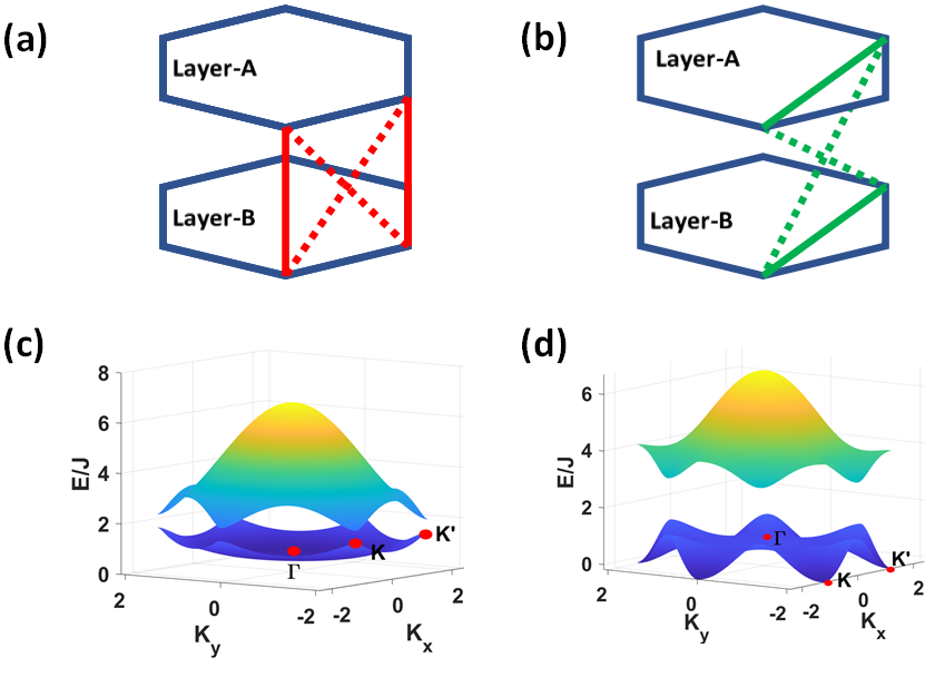
We start with a $S=1/2$ Heisenberg antiferromagnet on a bilayer honeycomb lattice with out of plane exchange anisotropy and Dzyaloshinkii-Moriya interaction (DMI), schematically shown in Fig. 1(a) and described by the Hamiltonian,

$\mathbb{S}_{i,m}$ denotes the spin operator at $i$-th interlayer bond at layer $m$ ($m\in\{A,B\}$). $\langle\ldots\rangle$ and $\langle\langle\ldots\rangle\rangle$ denote the nearest-neighbor (NN) and next-nearest-neighbor (NNN) inter-dimer bonds respectively. $J_{\perp}(>0)$ is the strength of (isotropic) interlayer Heisenberg interaction, while $J_{z}$ ($>0$) and $J$ ($>0$) denote the Ising and XX type intralayer NN Heisenberg exchange interactions respectively. $D$ is the Dzyaloshinskii–Moriya interaction (DMI) which is constrained by the symmetry of the lattice to intralayer NNN bonds; $\nu_{ij}=+1$, if $i\to j$ forms part of a counterclockwise closed loop connecting the NNN sites in a hexagonal plaquette in each layer (see counterclockwise circular arrows in Fig. 1(a)-(b)) and $\nu_{ij}=-1$ otherwise. Finally $B_{z}S_{i,m}^{z}$ describes a Zeeman coupling between a local spin-moment and an external longitudinal magnetic field. It is noticeable that the change in sign of $J$ and $D$ do not alter the magnetic ground state as well as excitations above the ground state, whereas $J_{z}$ and $J_{\perp}$ are strictly positive in this study.

For $J_{\perp}\gg|J|$, the ground state of the system is a product of the singlet dimers on each interlayer NN bond. In this limit, the lowest excitations of the system are triplons, which are localized $S=1$ quasipartices. An out-of-plane magnetic field lowers the energy of the $S_{z}=+1$ triplons and at a critical magnetic field, it crosses the energy of the singlet state, populating the ground state with a finite density of triplons. The other triplon branches ($S^{z}=0$ and $S^{z}=-1$) are separated by a large energy gap. At low temperatures, one can restrict the local Hilbert space of the dimers to the singlet and $S^{z}=+1$ triplon. By treating the triplons as bosonic quasiparticles, one can formulate a description of the low energy physics of the system in terms of hard core bosons which is known as bond-operator formalism (see also Appendix.A). In this formalism, the zero field ground state made of singlets on each interlayer bonds is considered an empty lattice with number of triplons $n_{i}=0\;\forall i$. At the critical field, a finite density of triplons is generated which increases with increasing field. The inter-dimer exchange interactions induce an effective hopping of the triplons. This delocalization induces a BEC of $S_{z}=+1$ triplons in the ground state. In the spin language, this corresponds to an canted antiferromagnetic order with a spontaneously broken U(1) symmetry. Considering singlets as a vacuum state in the system and triplon ($S_{z}=+1$) as a hard-core bosonic quasi-particle excitations in vacuum of singlets, we can use the bond operator formalism to express the bi-layer spin Hamiltonian Eq. 1 as an effective triplon Hamiltonian on a single-layer honeycomb lattice Zapf et al. 2014; Sachdev and Bhatt 1990; Romhányi et al. 2011 (see Appendix. A),

where, $\hat{t}_{i}$ is the triplon annihilation operator, $\hat{n}_{i}$ is the triplon number operator and index-$i$ represents site index of effective single-layer honeycomb lattice (which is equivalent to interlayer bond-index of bi-layer honeycomb lattice). The first two terms represent hopping of triplons between NN and NNN neighbor dimers respectively, the third term is an on-site potential (effectively a chemical potential) and the last term describes the effects of NN interaction between triplons. It is noticeable that the NNN hopping has a complex weight which renders the Hamiltonian unsuitable for quantum Monte Carlo simulations. When $J_{z}\approx 0$, Eq.2 reduces to a tight binding model of non-interacting triplons. The Bloch Hamiltonian in the momentum basis, in terms of the momentum space triplon operators, is determined via Fourier transformation as,

where, $\Psi_{\mathbb{k}}=(\hat{a}_{\mathbb{k}},\hat{b}_{\mathbb{k}})^{T}$. $\hat{a}_{\mathbb{k}}$ ($\hat{b}_{\mathbb{k}}$) denotes the ${\bf k}$-space triplon annihilation operator on sublattice-a (b) as shown in Fig. 1(a)-(b) and $\bm{\sigma}$ is the pseudo-vector of Pauli matrices and $\sigma_{0}$ is the two-dimensional identity matrix. The coefficients of the $\sigma$-matrices in the Bloch Hamiltonian are $g(\mathbb{k})=(J_{\perp}/4)-B_{z}$, $h_{x}(\mathbb{k})=(J/2)\sum_{i}\cos(\bold{k}\cdot\boldsymbol{\alpha}_i)$, $h_{y}(\mathbb{k})=(J/2)\sum_{i}\sin(\bold{k}\cdot\boldsymbol{\alpha}_i)$, $h_{z}(\mathbb{k})=D\sum_{i}\sin(\bold{k}\cdot\boldsymbol{\beta}_i)$, where $\bm{\alpha}_{i}$ and $\bm{\beta}_{i}$ are the NN and NNN vectors for each layer respectively. $\bm{\beta}_{i}$’s are chosen such that they form a counter-clockwise triangular loop for sites in sublattice-a in a hexagonal plaquette and clockwise triangular loop for sites in sublattice-b. The energy eigenvalues are given by,

The band dispersion is shown in Fig. 1(c) and Fig. 1(d) for two values of DMI. For ${\bf D}=0$, the energy spectrum is identical to that of graphene, with a linear band crossing of the upper and lower bands at the Dirac points $K$ and $K^{\prime}$. A finite DMI breaks time reversal symmetry and opens a band-gap $6\sqrt{3}D$ at these points. The energy of the lower band at $\Gamma$ and $K$ ($K^{\prime}$)-points are respectively given by (at $B_{z}=0$),

In the absence of DMI, the energy minimum is located at the center of the Brillouin zone, the $\Gamma$ point. For a finite but small DMI, the band minimum remains at $\Gamma$-point (Fig. 1(c)). Increasing DMI to $|D|>|J|/\sqrt{3}$ shifts the band minimum from $\Gamma$-point to two degenerate minima at the $K$ and $K^{\prime}$ (Fig. 1(d)). Thus with changing DMI, the ground state changes from a one component BEC (condensation momentum ${\bf k}=0$) to a two component BEC (condensation momenta at k = $K$ and $K^{\prime}$). The transition happens at $|D|=|J|/\sqrt{3}$ independent of $J_{\perp}$ and $B_{z}$ for small $B_{z}$.

In presence of repulsive interaction between triplons ( the last term in Eq. 2 ) co-existence of triplons at $K$ and $K^{\prime}$ points costs no additional energy classically ( see Appendix. B ) , but the quantum-fluctuations around $\mathbb{K}$ and $\mathbb{K}^{\prime}$ points introduces an energy cost Li et al. 2014. Thus spontaneous breaking of valley-symmetry is energetically favoured and the quantum fluctuation will lead to a ground state with only single valley condensation which is known as “quantum order by disorder” effect Li et al. 2014; Adhikari et al. 2010; Henley 1989. Thus, in the limit of weak interaction, the super-fluid order parameter at lattice site $\mathbb{r}$ is either $|b|e^{i\mathbb{K}\cdot\mathbb{r}+\phi}$ or $|b|e^{i\mathbb{K}^{\prime}\cdot\mathbb{r}+\phi}$ depending on the valley for the Bose-Einstein condensate, where $\phi$ is a global phase independent of position of lattice site. This spontaneous breaking of valley symmetry transforms the superfluid order-parameter from a real to a complex value and the resultant BEC is known as twisted superfluid Jürgensen et al. 2015. Based on this, the ground state on the honeycomb lattice is no longer a bipartite lattice in twisted superfluid phase, but become a lattice with six-sublattices as shown in the figure Fig. 2. Results based on CGMFT also supports this scenario as shown in section Sec. III.

In absence of interaction $J_{z}$, Eq. 2 transforms into well-known bosonic topological Haldane model. At finite temperatures due to non-zero magnetic excitations, this model is known to exhibit a finite thermal Hall effect due to presence of non-zero Berry-curvature of the bands. On this basis it is expected that Bose-Einstein condensate at $\Gamma$-point or $K$ ($K^{\prime}$)-point would provide a non-zero Hall conductance even at zero temperature Li et al. 2014. However, we find that the Berry-curvature at the condensation momenta – $\Gamma$-point when $|D|<|J|/\sqrt{3}$ and $K$ ($K^{\prime}$)-point when $|D|>|J|/\sqrt{3}$ – is zero. Since the density of magnons is concentrated around the condensation momentum, and is vanishingly small away from it, the thermal Hall response of the Bose-Einstein condensate is vanishingly small in our model.

An analogous bosonic model can also be observed in terms of Matsubara-Matsuda bosons in magnetically ordered honeycomb ferromagnets (see Fig. 1(b) ) or antiferromagnets. Thus the non-trivial phases like twisted-superfluid or twisted-supersolid are also expected to emerge in magnetically ordered systems. However, in practice, the presence of anisotropies in magnetically ordered systems break the $U(1)$-symmetries destroying conservation of numbers of particles which in-turn preclude a long time superfluidity response in this systems Zapf et al. 2014; Giamarchi et al. 2008. Moreover due to presence of strong exchange interactions ($J,\,J_{z}$ in Eq. 2) in general, the phase transitions are also difficult to study varying the external parameters in these systems Giamarchi et al. 2008. That is why the dimerized paramagnets are well suited to study superfluid phases and superfluid-Mott transitions. Hence we focus on bilayer dimerized honeycomb paramagnetic system to study the twisted superfluid and twisted supersolid phases.

The cluster Gutzwiller mean field theory or CGMFT Lühmann 2013; Jürgensen et al. 2015 – equivalently, cluster mean field theory Chen and Yang 2017; Gelfand et al. 1989; Yamamoto et al. 2014; Moreno-Cardoner et al. 2014; Yamamoto et al. 2012a; Yamamoto et al. 2012b; Singh et al. 2014, self-consistent cluster mean field theory Hassan et al. 2007, multi-site mean field theory McIntosh et al. 2012, hierarchical mean field approach Isaev et al. 2009a; Isaev et al. 2009b, composite boson mean field theory Huerga et al. 2013 – is a powerful technique to study superfluid phases in bosonic many body systems with complex hopping terms. CGMFT improves over the conventional single-site mean field approach by taking into account the short range correlations present within a small lattice-cluster using exact-diagonalization. Furthermore it is an alternative numerical method to study the quantum systems like we described in section Sec. II, where sign problems arises in quantum Monte-Carlo methods due to complex hopping terms or geometric frustration Yamamoto et al. 2017; Huerga et al. 2014. Whereas conventional mean-field theories Choudhury and Mueller 2013 and exact-diagonalization of small systems Cao et al. 2015 fail to show existence of TSF and TSS phases, Density Matrix Renormalization Group for one dimensional systems Lühmann 2016 and CGMFT for higher dimensional systems Jürgensen et al. 2015 are better alternatives for search of these non-trivial phases.

We explore the ground state phases of the effective triplon Hamiltonian with CGMFT by decomposing the system into clusters (pink shaded region) and mean-field region (blue shaded region) as shown in figure Fig. 2. The effective mean-field Hamiltonian of the cluster is given as,

where, $\pazocal{H}_{C}$ is the Hamiltonian as in equation Eq.( 2) within the cluster and $\pazocal{H}_{\delta C}$ is the Hamiltonian which takes into account the interactions among the boundary sites of the cluster and the mean-field region. The form of the boundary Hamiltonian is given by,

where the primed summations are over the boundary site-$i$ connected to the mean-field site-$j$. $\left\langle\hat{t}_{j}\right\rangle$ and $\left\langle\hat{n}_{j}\right\rangle$ are two mean-field parameters denoting the superfluid order parameter and occupation number of triplons at site-$j$ respectively. We choose six inequivalent sites in each cluster (denoted by different patterns in figure Fig. 2) to give a total of 12 mean-field parameters. The ground state in the different parameter regimes are obtained by evaluating these mean field parameters self-consistently in the following manner,

• (i)

  Choose an initial set of mean field parameters $\left\{\left\langle\hat{t}_{j}\right\rangle,\,\left\langle\hat{n}_{j}\right\rangle\right\}$, $j=1,\dots,6$ and then exactly diagonalize the effective Hamiltonian of the cluster $\pazocal{H}^{\text{eff}}_{C}$.

• (ii)

  Calculate new mean field parameters $\left\langle\hat{t}^{\prime}_{j}\right\rangle$ and $\left\langle\hat{n}^{\prime}_{j}\right\rangle$ from the sites within blue-dashed rectangle in the figure Fig. 2 which reside within the cluster. Periodic boundary condition is chosen along horizontal direction to eliminate any boundary effect on the sites within the blue-dashed rectangle, so that the mean field parameters obtained from those sites are free from boundary effects.

• (iii)

  The initial and final set of mean field parameters are compared using the tolerance

  $$\epsilon=\sum_{j}\left|\left\langle\hat{t}^{\prime}_{j}\right\rangle-\left\langle\hat{t}_{j}\right\rangle\right|+\sum_{j}\left|\left\langle\hat{n}^{\prime}_{j}\right\rangle-\left\langle\hat{n}_{j}\right\rangle\right|.$$

  (8)

  If the tolerance $\epsilon$ is less than a certain cutoff then the obtained mean-field parameters correspond to the ground state of the system. Otherwise the step-(i) is repeated with new values of mean-field parameters $\left\langle\hat{t}_{j}\right\rangle=\left\langle\hat{t}^{\prime}_{j}\right\rangle$ and $\left\langle\hat{n}_{j}\right\rangle=\left\langle\hat{n}^{\prime}_{j}\right\rangle$.

We set the cutoff as $10^{-10}$ and start the simulation with different initial mean-field parameter sets for a fixed set of parameters $J$, $D$, $J_{\perp}$, $B_{z}$, and $J_{z}$. In general, the simulations with different initial mean field parameter sets give different ground-states at the boundary of two phases and we selected the phase with minimum energy as the ground state.

After obtaining the ground state via self-consistent determination of the mean field parameters, four order-parameters are calculated to identify the nature of the ground state phase of the system. The magnitude of superfluid order parameter is given by,

where max denotes maximum value of the parameter obtained out of six-sites within the dashed blue-border in Fig. 2. Additioally, the average number of particles per site $\left\langle n\right\rangle_{av}$ and difference in number of particles between NN sites $\Delta n$ are also enumerated. The superfluid order-parameter is a complex quantity and for twisted super-fluid phases in our study the phase difference of superfluid order parameter $b$ among NNN sites is obtained to be $\theta=120^{o}$ and otherwise $\theta=0^{o}$.

Using CGMFT, we determine the order parameters $|b|$, $\left\langle b\right\rangle_{av}$, $\Delta n$ and $\theta$ as a function of magnetic field $B_{z}$ for different sets of the parameters $(D,J_{z})$. The evolution of the order parameters and the resulting field driven phases are shown in Figure fig. 3 for four illustrative points of the $(D,J_{z})$ parameter space. In fig. 3, the DMI increases from the left-column of figures to the right-column of figures, whereas the interaction $J_{z}$ increases from upper-row of figures towards the lower-row of figures.

For weak DMI ($D=0.2J$), the field driven phase diagram resembles that of the canonical extended Bose Hubbard model for hard core bosons Gan et al. 2007 (see Fig. 3(a), (c)). The zero field ($B_{z}=0$) ground state corresponds to a singlet phase, or equivalently an empty lattice in the bosonic language. All the order parameters vanish in this limit. This remains true at small values of the applied field reflecting a finite gap to lowest excitations due to the singlet-triplet gap of the local dimers. When the applied field exceeds a critical value, the gap is closed and the ground state acquires a finite density of triplons. These field induced triplons form a superfluid (SF) driven by the NN triplon hopping and is characterised by a finite SF order parameter, $|b|$. The mismatch between the occupancy of the two sublattices ($\Delta n$) remains zero, reflecting the uniform nature of the SF phase. A vanishing twist angle ($\theta=0$) completes the characterization of the phase as a normal superfluid. In the weak interaction limit ($J_{z}<2J$) with increasing magnetic field, the density of triplons increases monotonically till full saturation is reached at an upper critical field when each dimer is occupied by a triplon. At saturation, all the order parameters (except average density, $\langle n\rangle_{av}$, of triplons) vanish denoting a lattice fully occupied by triplons. In this weak interaction limit, the physics is similar to the non-interacting limit as described in section II and so the qualitative feature can be well described using band structure as in figure Fig. 1(c).

For strong interactions ($J_{z}>2J$), an intervening charge density wave (CDW) phase, driven by the strong NN-interaction between triplons, appears in addition to the phases discussed above (see Fig. 3(c)). With increasing magnetic field, when the density of triplons reaches $\langle n\rangle_{av}=1/2$, the triplons form a staggered CDW pattern where one of the sublattices is fully occupied, while the other remains empty. The potential energy-cost due to nearest neighbor interaction is minimized as there are no nearest neighbor pairs. This is accompanied by a complete quenching of superfluidity, since any hopping of triplons will necessarily involve configurations with energetically costly multiple nearest neighbor pairs. The CDW phase has a finite gap to the addition of any more triplons and the density remains constant at $\langle n\rangle_{av}=1/2$ over a finite rage of applied field. This phase is characterized by a vanishing superfluid order, and a non-zero density mismatch between the two sublattices ($\Delta n$), reflecting the staggered order. When the increasing field strength reaches a critical value where the Zeeman energy gain due to increasing magnetization (equivalently, adding more triplons) exceeds the potential energy cost of nearest neighbor repulsion, the density of triplons starts to increase again, resulting in another normal SF phase. Finally, as the field is increased above a saturation value, $B_{sat}$, the ground state enters the fully polarized phase.

The above argument for the appearance of interaction driven CDW phase at half-filling does not apply for weak to moderate interaction strengths ($J_{z}<2J$), as the kinetic energy gain due to the delocalization of triplons exceeds the potential energy cost of NN-interactions.

The sequence of field-driven phase changes markedly for strong DMI. As shown earlier in Sec. II, in the non-interacting limit, the triplon band minimum shifts from the $\Gamma$ point to the $K$ and $K^{\prime}$ (Fig. 1(d)) and the BEC of triplons occur at finite momentum. A local minimum persists at the center of the Brillouin zone, and the energy gap between the triplon-sector and the singlet dimer sector, $E_{K}$ in Eq. 5 decreases with increasing DMI. This behavior persists in the presence of weak to moderate interaction ($J_{z}<2J$) and is reflected in Fig. 3(b). For the present choice of parameters, the energy of the lowest triplon excitation is vanishingly small. The triplon density acquires a finite value for an infinitesimally small $B_{z}$, and increases monotonically with the strength of the applied field. In this regime, the triplons form a superfluid ($|b|>0$). More interestingly, the complex NNN hopping process imparts a complex phase to the superfluid order parameter, as seen by a finite expectation value of the twist angle ($\theta\neq 0$). In other words, the ground state in this parameter range is a twisted superfluid (TSF). The triplon density increases monotonically, with the ground state remaining a TSF, till the fully polarized phase is reached at a saturation field, $B_{sat}$.

Finally in the strong DMI and strong interaction limit (see Fig. 3(d)),the twisted superfluid is replaced by a twisted supersolid phase, in addition to the appearance of an interaction-driven CDW phase at $\langle n\rangle_{av}=1/2$ over a finite range of applied field. In the twisted supersolid phase (TSS), the ground state is characterized by a finite $\Delta n$ (density mismatch between the two sublattices), in addition to a complex superfluid order parameter ($|b|\neq 0,\,\theta\neq 0,$). The finite density difference between two sublattices provide the diagonal order concurrently with the finite (twisted) superfluid ordering. It is surprising that the ground state exhibits TSS order even at low triplon densities. This is understood by recalling that the primary delocalization process in this parameter regime involves the DMI-induced intra-sublattice complex next-nearest-neighbor hopping. The strong NN-repulsion between the triplons further suppresses inter-sublattice hopping processes, resulting in a preferential occupation of one of the two sublattices at small densities.

The phase diagram in $B_{z}-D$ parameter space is shown in the figure Fig. 4 for two different values of interaction $J_{z}=J$ and $J_{z}=4.5J$. A comparison of the phase diagrams at moderate ($J_{z}<2J$) and strong ($J_{z}>2J$) interactions reveal,

• (i)

  Appearance of CDW phase at half-filling in the strong interaction limit. The CDW phase appears at half filling dividing the SF-region which appear at weak to moderate $J_{z}$ into two SF-regions.

• (ii)

  In the strong interaction limit the TSF phase is replaced by a TSS phase.

There are two main ingredients to realize TSF or TSS phases; firstly, a bilayer honeycomb valence bond state is required; secondly, a DMI greater than a critical value is required. Although, to the best of our knowledge, there are no materials described in the literature which satisfies our model, a rough idea is sketched here to obtain TSS or TSF phases based on the real materials $\text{Bi}{\vphantom{\text{X}}}_{\smash[t]{\text{3}}}\text{Mn}{\vphantom{\text{X}}}_{\smash[t]{\text{4}}}\text{O}{\vphantom{\text{X}}}_{\smash[t]{\text{12}}}\text{(}\text{NO}{\vphantom{\text{X}}}_{\smash[t]{\text{3}}}\text{)}$ and $\text{CrI}{\vphantom{\text{X}}}_{\smash[t]{\text{3}}}$.

The material $\text{Bi}{\vphantom{\text{X}}}_{\smash[t]{\text{3}}}\text{Mn}{\vphantom{\text{X}}}_{\smash[t]{\text{4}}}\text{O}{\vphantom{\text{X}}}_{\smash[t]{\text{12}}}\text{(}\text{NO}{\vphantom{\text{X}}}_{\smash[t]{\text{3}}}\text{)}$ consists of Mn⁴⁺ ions carrying spin $S=\frac{3}{2}$ arranged in a bilayer honeycomb lattice with A-A stacking. No magnetic ordering is observed down to the lowest temperatures. Theoretical studies indicate that the disordered magnetic state may be an interlayer dimer phase which is adiabatically connected to the direct products of singlets Zhang et al. 2016; Kandpal and van den Brink 2011; Zhang et al. 2014; Oitmaa and Singh 2012; Ganesh et al. 2011a, although a spin liquid phase cannot be completely ruled out Mulder et al. 2010; Wang 2010; Okumura et al. 2010; Clark et al. 2011; Cabra et al. 2011; Ganesh et al. 2011b; Albuquerque et al. 2011; CABRA et al. 2011; Mezzacapo and Boninsegni 2012; Li et al. 2012; Ganesh et al. 2013; Gong et al. 2013. If the ground state phase is a spin liquid, an interlayer dimer phase can be induced by applying a pressure along the perpendicular direction Ganesh et al. 2011b; Oitmaa and Singh 2012.

On the other hand, experimentally well studied van der Waals material $\text{CrI}{\vphantom{\text{X}}}_{\smash[t]{\text{3}}}$ is a honeycomb ferromagnet where Cr²⁺-ions carry spin-$\frac{1}{2}$ momentum forming a honeycomb lattice. This material has been well studied by tuning the number of layers Huang et al. 2017 as well as varying the pressure Li et al. 2019. It is shown that the interlayer antiferromagnetic Heisenberg exchange interaction changes linearly with the distance between two layers by application of pressure on the material and can be achieved a interlayer coupling twice as compared with the initial interlayer coupling Li et al. 2019. Although a valence bond state is not detected in $\text{CrI}{\vphantom{\text{X}}}_{\smash[t]{\text{3}}}$ (and there are indications of structural phase transition under pressure) Li et al. 2019, the pressure induced high interlayer coupling in $\text{CrI}{\vphantom{\text{X}}}_{\smash[t]{\text{3}}}$ motivates for searching of pressure induced valance bond states in a family of Van der Walls honeycomb magnets $\text{CrBr}{\vphantom{\text{X}}}_{\smash[t]{\text{3}}}$ Samuelsen et al. 1971, $\text{CrGeTe}{\vphantom{\text{X}}}_{\smash[t]{\text{3}}}$ Gong et al. 2017, $\text{CrSiTe}{\vphantom{\text{X}}}_{\smash[t]{\text{3}}}$ Williams et al. 2015, $\text{FePS}{\vphantom{\text{X}}}_{\smash[t]{\text{3}}}$ Lee et al. 2016, $\text{NiPS}{\vphantom{\text{X}}}_{\smash[t]{\text{3}}}$ Kuo et al. 2016.

Another challenge for achieving the TSF and TSS phases is to obtain a high DMI ($|D|>J/\sqrt{3}$). The materials $\text{Bi}{\vphantom{\text{X}}}_{\smash[t]{\text{3}}}\text{Mn}{\vphantom{\text{X}}}_{\smash[t]{\text{4}}}\text{O}{\vphantom{\text{X}}}_{\smash[t]{\text{12}}}\text{(}\text{NO}{\vphantom{\text{X}}}_{\smash[t]{\text{3}}}\text{)}$ and $\text{CrI}{\vphantom{\text{X}}}_{\smash[t]{\text{3}}}$ are experimentally predicted to possess DMI Okubo et al. 2012; Chen et al. 2018. However the magnitude of DMI is small for realizations TSS and TSF states. This problem can be overcome by application of circularly polarized light. A circularly polarized light couples either to the charge Vinas Boström et al. 2020 or to the magnetic degrees of freedom Owerre 2017 and it has been shown theoretically that both kinds of mechanisms give rise to scalar spin chiral interaction in a honeycomb magnetic insulator. The synthetic scalar spin chiral interaction as in reference Ref. Vinas Boström et al. 2020 given by,

where the $i$-th site is the NNN neighbor of both $j$-th and $k$-th sites, $\chi$ is synthetic scalar spin chirality. Comparing the equations Eq. 2 and Eq. 10, the effective DMI for bond $\left\langle\left\langle jk\right\rangle\right\rangle$ due to circularly polarized light is $D=\frac{3\chi\left\langle n_{i}\right\rangle}{2}$. The scalar spin chirality $\chi$ is shown to have a resonance for the frequency of light near $\omega_{n}=\frac{1}{\hbar}\frac{U}{n}$, where $U$ is onsite interaction representing electron-electron repulsion and $n$ is a positive integer. Thus the effective DMI can be tuned as high as possible tuning the frequency of the light nearby $\omega_{n}$. However the results in Ref. Vinas Boström et al. 2020 is based on single-band extended Hubbard model; for a magnetic material which cannot be described by a one band Hubbard model, one needs a more careful theoretical treatment. On the other hand, application of light may not be required for a real material if the cutoff of DMI to realize TSF or TSS states is reduced due to presence of frustration among interlayer and intralayer interactions (see Appendix. C).

To summarize, we have shown that a magnetic analog of the novel twisted superfluid (TSF) state reported in recent experiments with ultracold atoms in an optical lattice Soltan-Panahi et al. 2011 can be realized in a bilayer quantum antiferromagnet with realistic interactions. We show that TSF phase is induced by DMI greater than a critical value. For Ising-like anisotropy of the intra-plane Heisenberg interactions, the TSF phase is replaced by a twisted supersolid (TSS) phase. While the strength of DMI required for the stabilization of TSF and TSS phases ($D/J\gtrsim 0.5$) is not observed natively in most quantum magnets, recent experiments have shown that a strong DMI can be induced in thin films of insulating magnets, by forming heterostructures with heavy metals (with strong spin-orbit coupling) Tacchi et al. 2017; Heide et al. 2008; Di et al. 2015; Gastaldo et al. 2019. Our results show that circularly polarized light can also induce large DMI by varying the frequency of light Vinas Boström et al. 2020. Finally, the presence of frustration among interlayer and intralayer Heisenberg exchange interactions in a material can lower the value of the critical DMI required to realize TSF and TSS phases (Appendix. C), thus facilitating their experimental observation. We propose that the material $\text{Bi}{\vphantom{\text{X}}}_{\smash[t]{\text{3}}}\text{Mn}{\vphantom{\text{X}}}_{\smash[t]{\text{4}}}\text{O}{\vphantom{\text{X}}}_{\smash[t]{\text{12}}}\text{(}\text{NO}{\vphantom{\text{X}}}_{\smash[t]{\text{3}}}\text{)}$ Zhang et al. 2016; Kandpal and van den Brink 2011; Zhang et al. 2014; Oitmaa and Singh 2012; Ganesh et al. 2011a and family of honeycomb magnets $\text{CrBr}{\vphantom{\text{X}}}_{\smash[t]{\text{3}}}$ Samuelsen et al. 1971, $\text{CrGeTe}{\vphantom{\text{X}}}_{\smash[t]{\text{3}}}$ Gong et al. 2017, $\text{CrSiTe}{\vphantom{\text{X}}}_{\smash[t]{\text{3}}}$ Williams et al. 2015, $\text{FePS}{\vphantom{\text{X}}}_{\smash[t]{\text{3}}}$ Lee et al. 2016, $\text{NiPS}{\vphantom{\text{X}}}_{\smash[t]{\text{3}}}$ Kuo et al. 2016 are promising candidate materials to realize TSF and TSS phases.

It is a pleasure to thank Oleg Sushkov for useful discussions. Financial support from the Ministry of Education, Singapore, in the form of grant MOE2018-T1-001-021 is gratefully acknowledged. A. Chatterjee acknowledges the financial support received from INSPIRE, Department of Science and Technology, Govt. of India and the NTU-India Connect Program. A. Chatterjee would like to thank the School of Physical and Mathematical Sciences at NTU for their kind hospitality.

References

- Soltan-Panahi et al. (2011) P. Soltan-Panahi, D.-S. Lühmann, J. Struck, P. Windpassinger, and K. Sengstock, Nature Physics 8, 71–75 (2011).
- Luke et al. (1998) G. M. Luke, Y. Fudamoto, K. M. Kojima, M. I. Larkin, J. Merrin, B. Nachumi, Y. J. Uemura, Y. Maeno, Z. Q. Mao, Y. Mori, and et al., Nature 394, 558–561 (1998).
- Wysokinski (2019) K. Wysokinski, Condensed Matter 4, 47 (2019).
- Luke et al. (1993) G. M. Luke, A. Keren, L. P. Le, W. D. Wu, Y. J. Uemura, D. A. Bonn, L. Taillefer, and J. D. Garrett, Phys. Rev. Lett. 71, 1466 (1993).
- Kaur and Agterberg (2003) R. P. Kaur and D. F. Agterberg, Phys. Rev. B 68, 100506(R) (2003).
- Kaminski et al. (2002) A. Kaminski, S. Rosenkranz, H. Fretwell, J. C. Campuzano, Z. Li, H. Raffy, W. Cullen, H. You, C. Olson, C. Varma, and H. Höchst, Nature 416, 610 (2002).
- Jürgensen et al. (2015) O. Jürgensen, K. Sengstock, and D.-S. Lühmann, Scientific Reports 5, 12912 (2015).
- Tanaka et al. (2001) H. Tanaka, A. Oosawa, T. Kato, H. Uekusa, Y. Ohashi, K. Kakurai, and A. Hoser, Journal of the Physical Society of Japan 70, 939 (2001).
- Coldea et al. (2003) R. Coldea, D. A. Tennant, and Z. Tylczynski, Phys. Rev. B 68, 134424 (2003).
- Singh and Johnston (2007) Y. Singh and D. C. Johnston, Phys. Rev. B 76, 012407 (2007).
- Demokritov et al. (2006) S. Demokritov, V. Demidov, O. Dzyapko, G. Melkov, A. Serga, B. Hillebrands, and A. Slavin, Nature 443, 430 (2006).
- Dzyapko et al. (2007) O. Dzyapko, V. Demidov, S. Demokritov, G. Melkov, and A. Slavin, New Journal of Physics 9, 64 (2007).
- Bradley et al. (1995) C. C. Bradley, C. A. Sackett, J. J. Tollett, and R. G. Hulet, Phys. Rev. Lett. 75, 1687 (1995).
- Davis et al. (1995) K. B. Davis, M. O. Mewes, M. R. Andrews, N. J. van Druten, D. S. Durfee, D. M. Kurn, and W. Ketterle, Phys. Rev. Lett. 75, 3969 (1995).
- Zapf et al. (2014) V. Zapf, M. Jaime, and C. D. Batista, Rev. Mod. Phys. 86, 563 (2014).
- Sachdev and Bhatt (1990) S. Sachdev and R. N. Bhatt, Phys. Rev. B 41, 9323 (1990).
- Romhányi et al. (2011) J. Romhányi, K. Totsuka, and K. Penc, Phys. Rev. B 83, 024413 (2011).
- Li et al. (2014) X. Li, S. S. Natu, A. Paramekanti, and S. D. Sarma, Nature Communications 5, 5174 (2014).
- Adhikari et al. (2010) S. K. Adhikari, B. A. Malomed, L. Salasnich, and F. Toigo, Phys. Rev. A 81, 053630 (2010).
- Henley (1989) C. L. Henley, Phys. Rev. Lett. 62, 2056 (1989).
- Giamarchi et al. (2008) T. Giamarchi, C. Rüegg, and O. Tchernyshyov, Nature Physics 4, 198–204 (2008).
- Lühmann (2013) D.-S. Lühmann, Phys. Rev. A 87, 043619 (2013).
- Chen and Yang (2017) Y.-C. Chen and M.-F. Yang, Journal of Physics Communications 1, 035009 (2017).
- Gelfand et al. (1989) M. P. Gelfand, R. R. P. Singh, and D. A. Huse, Phys. Rev. B 40, 10801 (1989).
- Yamamoto et al. (2014) D. Yamamoto, G. Marmorini, and I. Danshita, Phys. Rev. Lett. 112, 127203 (2014).
- Moreno-Cardoner et al. (2014) M. Moreno-Cardoner, H. Perrin, S. Paganelli, G. De Chiara, and A. Sanpera, Phys. Rev. B 90, 144409 (2014).
- Yamamoto et al. (2012a) D. Yamamoto, I. Danshita, and C. A. R. Sá de Melo, Phys. Rev. A 85, 021601(R) (2012a).
- Yamamoto et al. (2012b) D. Yamamoto, A. Masaki, and I. Danshita, Phys. Rev. B 86, 054516 (2012b).
- Singh et al. (2014) M. Singh, T. Mishra, R. V. Pai, and B. P. Das, Phys. Rev. A 90, 013625 (2014).
- Hassan et al. (2007) S. R. Hassan, L. de Medici, and A. M. S. Tremblay, Phys. Rev. B 76, 144420 (2007).
- McIntosh et al. (2012) T. McIntosh, P. Pisarski, R. J. Gooding, and E. Zaremba, Phys. Rev. A 86, 013623 (2012).
- Isaev et al. (2009a) L. Isaev, G. Ortiz, and J. Dukelsky, Phys. Rev. B 79, 024409 (2009a).
- Isaev et al. (2009b) L. Isaev, G. Ortiz, and J. Dukelsky, Phys. Rev. Lett. 103, 177201 (2009b).
- Huerga et al. (2013) D. Huerga, J. Dukelsky, and G. E. Scuseria, Phys. Rev. Lett. 111, 045701 (2013).
- Yamamoto et al. (2017) D. Yamamoto, H. Ueda, I. Danshita, G. Marmorini, T. Momoi, and T. Shimokawa, Phys. Rev. B 96, 014431 (2017).
- Huerga et al. (2014) D. Huerga, J. Dukelsky, N. Laflorencie, and G. Ortiz, Phys. Rev. B 89, 094401 (2014).
- Choudhury and Mueller (2013) S. Choudhury and E. J. Mueller, Phys. Rev. A 87, 033621 (2013).
- Cao et al. (2015) L. Cao, S. Krönke, J. Stockhofe, J. Simonet, K. Sengstock, D.-S. Lühmann, and P. Schmelcher, Phys. Rev. A 91, 043639 (2015).
- Lühmann (2016) D.-S. Lühmann, Phys. Rev. A 94, 011603(R) (2016).
- Gan et al. (2007) J. Y. Gan, Y. C. Wen, J. Ye, T. Li, S.-J. Yang, and Y. Yu, Phys. Rev. B 75, 214509 (2007).
- Zhang et al. (2016) H. Zhang, C. A. Lamas, M. Arlego, and W. Brenig, Physical Review B 93, 235150 (2016).
- Kandpal and van den Brink (2011) H. C. Kandpal and J. van den Brink, Phys. Rev. B 83, 140412(R) (2011).
- Zhang et al. (2014) H. Zhang, M. Arlego, and C. A. Lamas, Phys. Rev. B 89, 024403 (2014).
- Oitmaa and Singh (2012) J. Oitmaa and R. R. P. Singh, Phys. Rev. B 85, 014428 (2012).
- Ganesh et al. (2011a) R. Ganesh, S. V. Isakov, and A. Paramekanti, Phys. Rev. B 84, 214412 (2011a).
- Mulder et al. (2010) A. Mulder, R. Ganesh, L. Capriotti, and A. Paramekanti, Phys. Rev. B 81, 214419 (2010).
- Wang (2010) F. Wang, Phys. Rev. B 82, 024419 (2010).
- Okumura et al. (2010) S. Okumura, H. Kawamura, T. Okubo, and Y. Motome, Journal of the Physical Society of Japan 79, 114705 (2010).
- Clark et al. (2011) B. K. Clark, D. A. Abanin, and S. L. Sondhi, Phys. Rev. Lett. 107, 087204 (2011).
- Cabra et al. (2011) D. C. Cabra, C. A. Lamas, and H. D. Rosales, Phys. Rev. B 83, 094506 (2011).
- Ganesh et al. (2011b) R. Ganesh, D. N. Sheng, Y.-J. Kim, and A. Paramekanti, Phys. Rev. B 83, 144414 (2011b).
- Albuquerque et al. (2011) A. F. Albuquerque, D. Schwandt, B. Hetényi, S. Capponi, M. Mambrini, and A. M. Läuchli, Phys. Rev. B 84, 024406 (2011).
- CABRA et al. (2011) D. C. CABRA, C. A. LAMAS, and H. D. ROSALES, Modern Physics Letters B 25, 891 (2011).
- Mezzacapo and Boninsegni (2012) F. Mezzacapo and M. Boninsegni, Phys. Rev. B 85, 060402(R) (2012).
- Li et al. (2012) P. H. Y. Li, R. F. Bishop, D. J. J. Farnell, and C. E. Campbell, Phys. Rev. B 86, 144404 (2012).
- Ganesh et al. (2013) R. Ganesh, J. van den Brink, and S. Nishimoto, Phys. Rev. Lett. 110, 127203 (2013).
- Gong et al. (2013) S.-S. Gong, D. N. Sheng, O. I. Motrunich, and M. P. A. Fisher, Phys. Rev. B 88, 165138 (2013).
- Huang et al. (2017) B. Huang, G. Clark, E. Navarro-Moratalla, D. R. Klein, R. Cheng, K. L. Seyler, D. Zhong, E. Schmidgall, M. A. McGuire, D. H. Cobden, and et al., Nature 546, 270–273 (2017).
- Li et al. (2019) T. Li, S. Jiang, N. Sivadas, Z. Wang, Y. Xu, D. Weber, J. E. Goldberger, K. Watanabe, T. Taniguchi, C. J. Fennie, and et al., Nature Materials 18, 1303–1308 (2019).
- Samuelsen et al. (1971) E. J. Samuelsen, R. Silberglitt, G. Shirane, and J. P. Remeika, Phys. Rev. B 3, 157 (1971).
- Gong et al. (2017) C. Gong, L. Li, Z. Li, H. Ji, A. Stern, Y. Xia, T. Cao, W. Bao, C. Wang, Y. Wang, and et al., Nature 546, 265–269 (2017).
- Williams et al. (2015) T. J. Williams, A. A. Aczel, M. D. Lumsden, S. E. Nagler, M. B. Stone, J.-Q. Yan, and D. Mandrus, Phys. Rev. B 92, 144404 (2015).
- Lee et al. (2016) J.-U. Lee, S. Lee, J. H. Ryoo, S. Kang, T. Y. Kim, P. Kim, C.-H. Park, J.-G. Park, and H. Cheong, Nano Letters 16, 7433 (2016).
- Kuo et al. (2016) C.-T. Kuo, M. Neumann, B. Karuppannan, H. Park, S. Kang, H. Shiu, J. Kang, B. Hong, M. Han, T. Noh, and J.-G. Park, Scientific Reports 6, 20904 (2016).
- Okubo et al. (2012) S. Okubo, T. Ueda, H. Ohta, W. Zhang, T. Sakurai, N. Onishi, M. Azuma, Y. Shimakawa, H. Nakano, and T. Sakai, Phys. Rev. B 86, 140401(R) (2012).
- Chen et al. (2018) L. Chen, J.-H. Chung, B. Gao, T. Chen, M. B. Stone, A. I. Kolesnikov, Q. Huang, and P. Dai, Phys. Rev. X 8, 041028 (2018).
- Vinas Boström et al. (2020) E. Vinas Boström, M. Claassen, J. McIver, G. Jotzu, A. Rubio, and M. Sentef, SciPost Physics 9, 061 (2020).
- Owerre (2017) S. A. Owerre, Journal of Physics Communications 1, 021002 (2017).
- Tacchi et al. (2017) S. Tacchi, R. E. Troncoso, M. Ahlberg, G. Gubbiotti, M. Madami, J. Åkerman, and P. Landeros, Phys. Rev. Lett. 118, 147201 (2017).
- Heide et al. (2008) M. Heide, G. Bihlmayer, and S. Blügel, Phys. Rev. B 78, 140403(R) (2008).
- Di et al. (2015) K. Di, V. L. Zhang, H. S. Lim, S. C. Ng, M. H. Kuok, J. Yu, J. Yoon, X. Qiu, and H. Yang, Phys. Rev. Lett. 114, 047201 (2015).
- Gastaldo et al. (2019) D. Gastaldo, N. Strelkov, L. D. Buda-Prejbeanu, B. Dieny, O. Boulle, P. Allia, and P. Tiberto, Journal of Applied Physics 126, 103905 (2019).