Quantum phase transition in a non-Hermitian XY spin chain with global complex transverse field

Quantum XY spin chain is a textbook model in exploring quantum magnetism and quantum phase transitions (QPTs) Sachdev 2011. It is extended from one-dimensional transverse field Ising model by adding the spin-spin interaction along another direction. There are two types of QPTs in the XY model, i.e., Ising phase transition Pfeuty 1970; Barouch and McCoy 1971 and anisotropic phase transition Barouch and McCoy 1971; Lieb et al. 1961; Latorre et al. 2004, which can be characterized by different critical behaviors. Since most XY models and their derivatives can be analytically solved by Jordan-Wigner transformation Jordan and Wigner 1928 or numerically solved by the renormalization group method Wilson 1983; Jullien et al. 1978; Jullien and Pfeuty 1979; Kargarian et al. 2008, XY model has attracted wide attention and fruitful research results have been obtained during the past decades Tong and Zhong 2001; Latorre et al. 2004; Mofidnakhaei et al. 2018; Zhang et al. 2017; Zhang and Song 2015; Bunder and McKenzie 1999; Zhong and Tong 2010; Zhong et al. 2013; Marzolino and Prosen 2017; Gao et al. 2017; Zhu 2006; Bi et al. 2021. On the other hand, great attention has been paid to the non-Hermitian systems as experimental techniques develop rapidly in recent years. Not only can non-Hermitian systems be readily realized through multiple existing table-top experimental platforms (such as cold atomic system Li et al. 2019; Li et al. 2020, optical system Chen et al. 2017; Peng et al. 2014; Cerjan et al. 2019, nitrogen-vacancy center Wu et al. 2019, etc.), but they can also trigger many novel physical phenomena (such as real eigenvalues with parity-time ($\mathcal{PT}$) symmetry Bender and Boettcher 1998, non-Hermitian skin effect Yao and Wang 2018; Yao et al. 2018, new topological properties corresponding to exceptional points (EPs) Zhang et al. 2020a; He et al. 2020; Shen et al. 2018; Bergholtz et al. 2021; Ghatak and Das 2019; Kawabata et al. 2019; He and Chien 2020 and disorders Zhang et al. 2020b; Luo and Zhang 2019; Tang et al. 2020; Jiang et al. 2019). What would happen if QPTs meet non-Hermitian effects?

In general, QPTs fall into two broad categories: traditional QPTs Sachdev 2011; Lee and Chan 2014; Yamamoto et al. 2019; Sun and Kou 2020 and topological QPTs Qi and Zhang 2011; Hasan and Kane 2010; Zhang et al. 2019; Tan et al. 2019; Wang et al. 2019; Zhu et al. 2013. The former can be depicted by local order parameters, while the latter are characterized by the global topological invariants. The non-Hermiticity gives rise to a brand-new phase transition, so called as non-Hermitian QPTs, characterized by energy spectrum. The new phase transition is closely related to particular symmetries, for instance, $\mathcal{PT}$ symmetry and intrinsic rotation-time-reversal ($\mathcal{RT}$) symmetry Zhang and Song 2013a; Wang et al. 2020; Lee and Chan 2014; Li et al. 2014; Zhang and Song 2020. The system features pure real energy spectrum in symmetry-preserving region, whereas it possesses complex energy spectrum in the region of broken symmetry Zhang and Song 2013a; Wang et al. 2020. Recent years have witnessed extensive investigation of the non-Hermitian QPTs and there are also some works for the spin system in the complex field or with the non-Hermitian interactions Nishiyama 2020a; Nishiyama 2020b; Zhang and Song 2013b; Bi et al. 2021. However, the research remains inadequate on the influence of non-Hermiticity on the traditional QPTs in spin system. Recently, there are some works that investigated non-Hermitian quantum criticality in real-spectrum region by biorthogonal fidelity susceptibility Sun and Kou 2020; Tzeng et al. 2021. But it is still an open question that how the non-Hermiticiy affects the traditional QPT and quantum magnetism in the complex-spectrum region or the system without $\mathcal{PT}$ or $\mathcal{RT}$ symmetry.

This paper is devoted to the research on the traditional QPTs in the presence of non-Hermitian effects, which are derived from global complex transverse field. First, we define the non-Hermitian ground state and energy gap. Based on characteristics of the energy gap, phase diagram of the system can be divided into three regions, which are corresponding to pure real gap, pure imaginary gap and complex gap, respectively. Besides, all gapless points form an exceptional ring. By studying the non-analyticity of the ground state energy density, we find that the phase transition which occurs on the exceptional ring is actually a second-order phase transition. Moreover, through the exact solution and numerical fitting, we investigate the long-range correlation function (LRCF) in different regions of the phase diagram. We discover the corresponding relations among the QPT, non-Hermitian energy gap and LRCF, i.e., ferromagnetic phase (critical transition zone, paramagnetic phase) corresponds to pure real (pure imaginary, complex) gap, whose LRCF features no decay (polynomial decay, exponential decay).

The paper is organized as follows. In Sec. 2, the model, the exact solution and its non-Hermitain ground state are provided. In Sec. 3, we define the non-Hermitian gap, draw the phase diagram and point out that the QPT on the exceptional ring is the second-order phase transition. In Sec. 4, we study the LRCF and analyze its decay behavior. Sec. 5 is the conclusion.

The Hamiltonian of a non-Hermitian quantum XY spin chain with a global complex transverse field reads

where $N$ denotes the total sites number of the chain. Since $N$ is large enough, $N/2$ could be considered a “decent half” no matter $N$ is even or odd. The Hilbert space on each site has a set of basis vectors of two spin states, i.e., $\ket{\uparrow}$ and $\ket{\downarrow}$. $\sigma_{j}^{x}$, $\sigma_{j}^{y}$ and $\sigma_{j}^{z}$ are the Pauli matrices for spin $j$ and $\sigma^{u}$ denotes the matrix $\bigl[\begin{smallmatrix}1&0\\ 0&0\end{smallmatrix}\bigr]$, which corresponds to the gain ($\Gamma<0$) or loss ($\Gamma>0$) of $\ket{\uparrow}$ with the rate of $\Gamma/2$. The system can be reduced to Hermitian XY model when $\Gamma=0$. $\lambda$ parameterizes transverse magnetic field along $z$ direction. $J$ ($\gamma$) represents the isotropic (anisotropic) nearest neighboring interaction strength between $x$ and $y$ directions. All the parameters are real numbers. The sign of $J$ determines that the system is characterized by ferromagnetic or antiferromagnetic chains. Since we hereby just concentrate on the ferromagnetism case, $J>0$ and $\gamma/J\in[-1,1]$ are taken into consideration. Besides, $J$ as the system character parameter is set as unit 1 later in this paper.

We can diagonalize the Hamiltonian in Eq. (1) by three steps. First, we map spin operators onto spinless Fermi operators by Jordan-Wigner transformation, i.e.,

where $\sigma=\bigl[\begin{smallmatrix}0&0\\ 1&0\end{smallmatrix}\bigr]$, $\sigma^{\dagger}=\bigl[\begin{smallmatrix}0&1\\ 0&0\end{smallmatrix}\bigr]$, and $c_{j}$ ($c_{j}^{\dagger}$) denotes the annihilation (creation) operators of the fermion on the $jth$ site. Then, we can obtain the Hamiltonian in the spinless fermion representation as

Second, we do Fourier transformation with $c_{k}=\frac{e^{i\pi/4}}{\sqrt{N}}\sum_{j}\text{exp}(-ikj)c_{j}$. The corresponding Hamiltonian in momentum space reads,

$\mathcal{H}(k)$ is the BdG Hamiltonian,

where the $\tau_{i}$ ($i=x,y,z$) is the Pauli matrix of pseudo spin and

Third, we use non-Hermitian Bogoliubov transformation to complete diagonalization of Hamiltonian in Eq. (4) following the method outlined in Ref. Lee and Chan 2014. In Ref. Lee and Chan 2014, the authors investigate nonequilibrium steady state, which has minimum imaginary part of eigenvalue. Here, we focus on the state with minimum real part of energy, which is defined as the non-Hermitian ground state in this paper. Thus, our definitions of the $u$, $v$ factors of Bogoliubov transformation are different from that in Ref. Lee and Chan 2014.

We define the annihilation ($\alpha$) and creation ($\bar{\alpha}$) operators of non-Hermitian Bogoliubov quasiparticles as

The $u$, $v$ factors are defined as $u_{k}=\cos{(\theta_{k}/2)}$ and $v_{k}=\sin{(\theta_{k}/2)}$ with the relations $\sin{\theta_{k}}=d_{x}(k)/E_{k}$, $\cos{\theta_{k}}=d_{z}(k)/E_{k}$, where

Then, the Hamiltonian is diagonalized as

Note that, since $u$, $v$ are complex numbers, $\alpha_{k}^{\dagger}\neq\bar{\alpha}_{k}$. The fermionic commutation relation is still held, i.e., $\{\bar{\alpha}_{k},\alpha_{k^{\prime}}\}=\delta_{kk^{\prime}}$ and $\{\alpha_{k},\alpha_{k^{\prime}}\}=\{\bar{\alpha}_{k},\bar{\alpha}_{k^{\prime}}\}=0$. As for the excited state energy $E_{k}$, we choose the branch cut of square root along the negative x-axis so that the real part of $E_{k}$ is always nonnegative. Therefore, we can define the non-Hermitian ground state $|G\rangle$ as the state with the minimum real part of energy. $|G\rangle$ can be obtained by the equation $\alpha_{k}|G\rangle=\alpha_{-k}|G\rangle=0$, i.e.,

where $|0\rangle$ is the vacuum state, $\mathcal{N}=\prod_{k=0}^{\pi}(|u_{k}|^{2}+|v_{k}|^{2})$ and the ground state energy $E_{G}$ is given as

Due to the nature of non-Hermiticity, the excited state $\bar{\alpha}_{\pm k}|0\rangle$ has a complex energy $E_{k}$ described in Eq. (8). Notably, the $E_{k}$ have nonnegative real part by the negative-x-axis branch cut of square root, so we can find a momentum $k_{m}$ to corresponds to the least real part of excitation energy, i.e., minimum value of ${\rm Re}[E(k_{m})]$. We define the minimum value as the non-Hermitian gap, which is denote as $\Delta$. In Hermitian systems, gapless points are usually the boundary of different phases. A natural question is whether the $\Delta$ will also become a landmark in non-Hermitian systems. Therefore, we divide the parameter space $(\lambda,\gamma,\Gamma)$ of the Hamiltonian (1) by $\Delta$.

First, by solving the equation $E_{k}=0$, one can get

The Eq. (12a) depicts an elliptical exceptional ring, and the Eq. (12b) implies a limitation $|\lambda|\leq J$. Therefore, the system can be separated into three regions as shown in Fig. 1.

Region I: $|\lambda|>J$. This region is characterized by a complex gap with ${\rm Re}[\Delta]>0$ and $|{\rm Im}[\Delta]|=|\Gamma|/2$, where the ${\rm Re}[\Delta]$ and ${\rm Im}[\Delta]$ represent the real and imaginary part of complex gap $\Delta$, respectively. We take $\lambda>J$ as an example. Under this condition, $k_{m}=\pi$ and $\Delta=2\lambda-2J+i\Gamma/2$.

Region II: inside the exceptional ring. This region has pure real gap, i.e., ${\rm Re}[\Delta]>0$ and ${\rm Im}[\Delta]=0$. In this region, $k_{m}=\arccos(-\frac{\lambda}{J})$ and $\Delta=\sqrt{4\gamma^{2}(1-\lambda^{2}/J^{2})-\Gamma^{2}/4}$.

Region III: outside the exceptional ring and $|\lambda|<J$. The gap is pure imaginary number (${\rm Re}[\Delta]=0$ and ${\rm Im}[\Delta]\neq 0$). In this region, we still have $k_{m}=\arccos(-\frac{\lambda}{J})$. However, $\Delta$ becomes a pure imaginary number because the non-Hermitian strength $\Gamma$ is large enough to be dominant, then $\Delta=\pm i\sqrt{\Gamma^{2}/4-4\gamma^{2}(1-\lambda^{2}/J^{2})}$.

Second, we investigate non-analyticity of ground state energy density $U_{G}$, which implies a QPT at zero temperature. Under the thermodynamic limit, we have

Moreover, the corresponding first-order derivatives reads

and the second-order derivatives can be obtained as

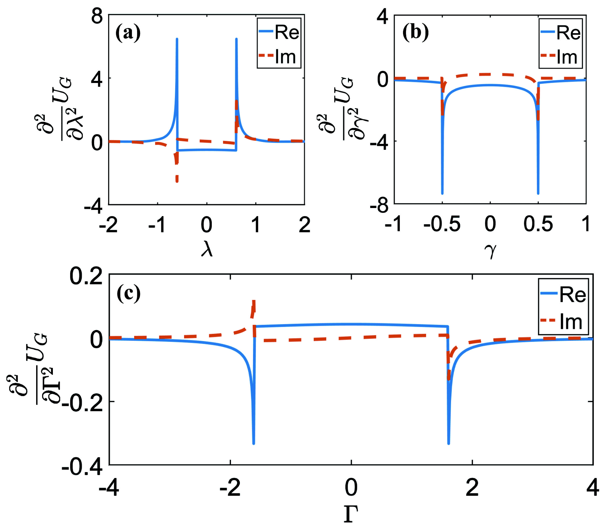
By numerical calculations, we find that $U_{G}$ and its first derivatives are continuous while there are divergent points in the second derivatives. The results of second derivatives are plotted in Fig. 2. It is obvious that the second derivatives diverge at the exceptional point $C_{0}$, which implies that a second-order QPT occurs on the exceptional ring.

The LRCFs are the order parameters of magnetic system in Hermitian spin models. For example, in ferromagnetic phase, LRCF $C_{xx}(r)=\langle G|\sigma_{0}^{x}\sigma_{r}^{x}|G\rangle$ or $C_{yy}(r)=\langle G|\sigma_{0}^{y}\sigma_{r}^{y}|G\rangle$ is a non-zero constant, where the parameter $r$ represents the distance between two spins. In paramagnetic phase, LRCF decays exponentially with the increase of $r$. At critical points, correlation functions have asymptotic behavior of polynomial decay, i.e. $C_{xx}(r)\propto r^{2-d-\eta}$, where $d$ and $\eta$ denote the spatial dimension and the critical exponent, respectively. $\eta$ varies in different universality classes. As for XY spin chain, $\eta$ is $5/4$ for the Ising phase transition at $\lambda/J=1$ and $3/2$ for the anisotropic phase transition at $\gamma=0$ Zhong and Tong 2010; Bunder and McKenzie 1999.

In our model, $C_{xx}(r)$ can be calculated through the Pfaffian of a $2r\times 2r$ skew symmetric matrix $\rm M$ ($\rm M^{\mathrm{T}}=-M$) Lee and Chan 2014

where the “ pf ” means the Pfaffian of a matrix. The numerical calculation codes for Pfaffian are from “Algorithm 923” Wimmer 2012. The elements of matrix $\rm M$ are as following:

The pair contractions for $A_{m}$ and $B_{n}$ are

It needs to be mentioned that in some works of non-Hermitian systems, the average value of an observable quantity is defined on the biorthogonal bases Brody 2013; Sternheim and Walker 1972. Here, we do not use the biorthogonal bases because we think it is not easy to measure the biorthogonal average value. The left and right eigenstate are not the same quantum state, thus before measuring the biorthogonal average value, one has to prepare two states, then finds a way to link the two states and the observable quantity together. These processes are inconvenient for experiments. Thus, in this work, the LRCF $C_{xx}(r)$ is only defined on conventional bases, i.e. the ground state $|G\rangle$ (Eq. 10) and its Hermitian conjugation $\langle G|$, and all the pair contractions in Eq.  20 are also based on conventional bases of the ground state.

From Eq. (16) to Eq. (20), we can obtain the exact value of $C_{xx}(r)$. Here, we show the values of $|C_{xx}(r)|$ in different $\lambda$ with $(J,\gamma,\Gamma)=(1,0.5,1.6)$. The data is plotted in Fig. 3. When $\lambda=1$ and $\lambda=1.2$, the system is in the region I and the LRCFs exponentially decay with the increase of $r$, which implies the system is in PM phase. When $\lambda=0.4$ and $\lambda=0.6$, the system is in the region II and the LRCFs are constants when $r$ is large, which shows the characteristic of FM phase.

An intriguing result which is unique for non-Hermitian case is obtained for the region III. When $\lambda=0.8$ and $\lambda=0.9$, the system is in the region III, the decay of $C_{xx}(r)$ is like polynomial type. In the Hermitian system, the polynomial decay only appears at critical point. In the non-Hermitian circumstances, the whole region III shows the similar behavior. Therefore, we call region III as CTZ. It is worth noting that, in Hermitian system, we can not distinguish ferromagnetic and paramagnetic phases only by energy gap. However, in this model, the different magnetic phases can be characterized by non-Hermitian gap.

To describe the decay more accurately, we fit data points in Fig. 3 by the function

where $A$, $B$, $C$ are the fitting parameters. Obviously, $C>0$ means an exponentially decay of correlation function, while the case $C=0$ and $B>0$ represents the polynomial decay. The fitting curves are shown by the black dashed lines in Fig. 3.

Now, we study the decay of $C_{xx}(r)$ by scanning the parameters across an exceptional point $C_{0}(\lambda=0.6,\,\gamma=0.5,\,\Gamma=1.6)$ along $\lambda$ and $\Gamma$. Fitting by Eq. (21), we get curves of parameters $A$, $B$, $C$ in Fig. 4 (a) and (b). In (a), $\lambda$ changes from $0.6$ to $1.2$. When $\lambda<1$, the system is in CTZ, where the red and blue curves show that $C=0$ and $B>0$. When $\lambda\geq 1$, the system is in region I, where the ground state is in PM phase characterized by $C>0$. In (b), we scan $\Gamma$ from $1.2$ to $2$, where $C$ is always equal to zero. When $\Gamma\leq 1.6$, the system is in region II and $B$ is near zero. Therefore, this region is corresponding to FM phase. In contrast, $B$ is obviously larger than zero when the system is in CTZ with $\Gamma>1.6$.

In CTZ, the parameter $C$ is always equal to zero so that the correlation function $|C_{xx}(r)|$ is proportional to $r^{-B}$. Compared with $C_{xx}(r)\propto r^{1-\eta}$ at critical points in Hermitian XY chain, we have that $\eta=1+B$. Fig. 4(d) and (e) show $\eta$ in CTZ with $\lambda\in[0.6,0.99]$ and $\Gamma\in[2,40]$, which reflect that non-Hermiticity influences critical behavior. When we change $\lambda$ in CTZ, $\eta$ is no longer standard value ($5/4$) of the Ising transition. When we increase $\Gamma$, $\eta$ tends to be near $3/2$, which corresponds to the anisotropic transition. It may imply that at large $\Gamma$ limit, the critical behavior of the non-Hermitian system is similar to the critical point of anisotropic transition. The intuitive explanation is that when $\Gamma$ is very large, the difference between the interactions in $x$ and $y$ directions, corresponding to $(J+\gamma)/2$ and $(J-\gamma)/2$, becomes comparatively insignificant.

In addition, we point out that the non-Hermitian term $i\frac{\Gamma}{2}\sigma^{u}_{j}$ does not influence anisotropic transition. This transition comes from the competition between $\frac{1}{2}(J+\gamma)\sigma^{x}_{j}\sigma^{x}_{j+1}$ and $\frac{1}{2}(J-\gamma)\sigma^{y}_{j}\sigma^{y}_{j+1}$. However, the non-Hermitian term is along $z$ direction ($\sigma^{u}=\frac{1}{2}(\mathbf{1}+\sigma^{z})$), which does not break the symmetry between $x$ and $y$ directions when $\gamma=0$. We show the fitting with $\gamma=0$ in Fig. 4 (c) and (f). It is obvious that $A$, $B$, $C$ and $\eta$ remain unchanged when we increase $\Gamma$. Furthermore, $\eta$ has always been $3/2$, which is same as the value of anisotropic transition in Hermitian XY chain.

At last, we mention the phase diagram again. In Sec.3 we study the derivatives of ground state energy density and find that non-analyticity is only on the EP ring, where the complex gap is equal to 0. This result seems to indicate that the system has only two phases, i.e. inside and outside the EP ring. In fact, by analyzing LRCFs, we find that there are three phases. An extra QPT occurs at the line with $|\lambda/J|=1$, where the gap is a pure imaginary number. This is a new property for non-Hermitian system that the QPT can occur without gap closing. The similar property has been found in the non-Hermitian Kitaev’s toric-code model Matsumoto et al. 2020.

Experimentally, the non-Hermitian XY model can be realized by some artificial quantum systems, such as ultracold atoms in optical lattices, superconducting qubits and coupled cavity arrays. For example, one can use three-level atoms in optical lattices to realize the required Hamiltonian. Two metastable states of atoms represent spin up and spin down. The Hermitian part of the system can be realized by arraying atoms in optical lattices Duan et al. 2003; Lee et al. 2013; Zhu et al. 2007. The non-Hermitian term can be generated by exciting one of the metastable states to an auxiliary state Li et al. 2019. Besides the cold atom experimental scheme mentioned above, the results can also be realized in coupled cavity arrays Joshi et al. 2013, in which the non Hermiticity can be realized by active and passive cavities Chang et al. 2014; Peng et al. 2014; Xing et al. 2017.

In summary, we have investigated the traditional QPT in a quantum XY spin chain with a global complex transverse field. This non-Hermitian transverse field changes the phase diagram of XY model. The results reveal that (i) the second-order QPT points change from Ising transition point to an exceptional ring. (ii) the critical points of Hermitian system are extended to a critical transition zone. In this zone, correlation function decays polynomially. Furthermore, the results reveal the correspondence among the different phases, non-Hermitian gap and LRCF.

Our results indicate the nontrivial influence of non-Hermiticity and our model offers a higher dimensional parameter space to study the critical behaviors and non-Hermitian quantum magnetism. Moreover, our findings in this paper can be readily realized with recent experimental techniques. We believe that our work will benefit the future research on traditional quantum phase transition of non-Hermitian systems.

We are grateful to S. L. Zhu for dedicated teaching and helpful discussions. This work was supported by the National Natural Science Foundation of China (Grants No. 12074180 and No. 11704132), the Key-Area Research and Development Program of GuangDong Province (Grant No. 2019B030330001), the Key Project of Science and Technology of Guangzhou (Grants No. 201804020055 and No. 2019050001).

References

- Sachdev (2011) S. Sachdev, Quantum Phase Transitions (2nd ed.) (Cambridge University Press, 2011).
- Pfeuty (1970) P. Pfeuty, The one-dimensional Ising model with a transverse field, Annals of Physics 57, 79 (1970).
- Barouch and McCoy (1971) E. Barouch and B. M. McCoy, Statistical Mechanics of the Model. II. Spin-Correlation Functions, Phys. Rev. A 3, 786 (1971).
- Lieb et al. (1961) E. Lieb, T. Schultz, and D. Mattis, Two soluble models of an antiferromagnetic chain, Annals of Physics 16, 407 (1961).
- Latorre et al. (2004) J. I. Latorre, E. Rico, and G. Vidal, Ground state entanglement in quantum spin chains, arXiv:quant-ph/0304098 (2004).
- Jordan and Wigner (1928) P. Jordan and E. Wigner, Über das Paulische Äquivalenzverbot, Zeitschrift für Physik 47, 631 (1928).
- Wilson (1983) K. G. Wilson, The renormalization group and critical phenomena, Rev. Mod. Phys. 55, 583 (1983).
- Jullien et al. (1978) R. Jullien, P. Pfeuty, J. N. Fields, and S. Doniach, Zero-temperature renormalization method for quantum systems. I. Ising model in a transverse field in one dimension, Phys. Rev. B 18, 3568 (1978).
- Jullien and Pfeuty (1979) R. Jullien and P. Pfeuty, Zero-temperature renormalization-group method for quantum systems. II. Isotropic model in a transverse field in one dimension, Phys. Rev. B 19, 4646 (1979).
- Kargarian et al. (2008) M. Kargarian, R. Jafari, and A. Langari, Renormalization of entanglement in the anisotropic Heisenberg model, Phys. Rev. A 77, 032346 (2008).
- Tong and Zhong (2001) P. Tong and M. Zhong, Quantum phase transitions of periodic anisotropic XY chain in a transverse field, Physica B: Condensed Matter 304, 91 (2001).
- Mofidnakhaei et al. (2018) F. Mofidnakhaei, F. Fumani, S. Mahdavifar, and J. Vahedi, Quantum correlations in anisotropic XY-spin chains in a transverse magnetic field, Phase Transitions 91, 1256 (2018).
- Zhang et al. (2017) G. Zhang, C. Li, and Z. Song, Majorana charges, winding numbers and Chern numbers in quantum Ising models, Scientific Reports 7, 8176 (2017).
- Zhang and Song (2015) G. Zhang and Z. Song, Topological Characterization of Extended Quantum Ising Models, Phys. Rev. Lett. 115, 177204 (2015).
- Bunder and McKenzie (1999) J. E. Bunder and R. H. McKenzie, Effect of disorder on quantum phase transitions in anisotropic XY spin chains in a transverse field, Phys. Rev. B 60, 344 (1999).
- Zhong and Tong (2010) M. Zhong and P. Tong, The Ising and anisotropy phase transitions of the periodic XY model in a transverse field, Journal of Physics A: Mathematical and Theoretical 43, 505302 (2010).
- Zhong et al. (2013) M. Zhong, H. Xu, X.-X. Liu, and P.-Q. Tong, The effects of the Dzyaloshinskii—Moriya interaction on the ground-state properties of theXYchain in a transverse field, Chinese Physics B 22, 090313 (2013).
- Marzolino and Prosen (2017) U. Marzolino and T. c. v. Prosen, Fisher information approach to nonequilibrium phase transitions in a quantum XXZ spin chain with boundary noise, Phys. Rev. B 96, 104402 (2017).
- Gao et al. (2017) Z.-P. Gao, D.-W. Zhang, Y. Yu, and S.-L. Zhu, Anti-Kibble-Zurek behavior of a noisy transverse-field chain and its quantum simulation with two-level systems, Phys. Rev. B 95, 224303 (2017).
- Zhu (2006) S.-L. Zhu, Scaling of Geometric Phases Close to the Quantum Phase Transition in the Spin Chain, Phys. Rev. Lett. 96, 077206 (2006).
- Bi et al. (2021) S. Bi, Y. He, and P. Li, Ring-frustrated non-Hermitian XY model, Physics Letters A 395, 127208 (2021).
- Li et al. (2019) J. Li, A. K. Harter, J. Liu, L. de Melo, Y. N. Joglekar, and L. Luo, Observation of parity-time symmetry breaking transitions in a dissipative Floquet system of ultracold atoms, Nature Communications 10, 855 (2019).
- Li et al. (2020) L. Li, C. H. Lee, and J. Gong, Topological Switch for Non-Hermitian Skin Effect in Cold-Atom Systems with Loss, Phys. Rev. Lett. 124, 250402 (2020).
- Chen et al. (2017) W. Chen, Ş. Kaya Özdemir, G. Zhao, J. Wiersig, and L. Yang, Exceptional points enhance sensing in an optical microcavity, Nature 548, 192 (2017).
- Peng et al. (2014) B. Peng, Ş. K. Özdemir, F. Lei, F. Monifi, M. Gianfreda, G. L. Long, S. Fan, F. Nori, C. M. Bender, and L. Yang, Parity-time-symmetric whispering-gallery microcavities, Nature Physics 10, 394 (2014).
- Cerjan et al. (2019) A. Cerjan, S. Huang, M. Wang, K. P. Chen, Y. Chong, and M. C. Rechtsman, Experimental realization of a Weyl exceptional ring, Nature Photonics 13, 623 (2019).
- Wu et al. (2019) Y. Wu, W. Liu, J. Geng, X. Song, X. Ye, C.-K. Duan, X. Rong, and J. Du, Observation of parity-time symmetry breaking in a single-spin system, Science 364, 878 (2019).
- Bender and Boettcher (1998) C. M. Bender and S. Boettcher, Real Spectra in Non-Hermitian Hamiltonians Having Symmetry, Phys. Rev. Lett. 80, 5243 (1998).
- Yao and Wang (2018) S. Yao and Z. Wang, Edge States and Topological Invariants of Non-Hermitian Systems, Phys. Rev. Lett. 121, 086803 (2018).
- Yao et al. (2018) S. Yao, F. Song, and Z. Wang, Non-Hermitian Chern Bands, Phys. Rev. Lett. 121, 136802 (2018).
- Zhang et al. (2020a) D.-W. Zhang, Y.-L. Chen, G.-Q. Zhang, L.-J. Lang, Z. Li, and S.-L. Zhu, Skin superfluid, topological Mott insulators, and asymmetric dynamics in an interacting non-Hermitian Aubry-André-Harper model, Phys. Rev. B 101, 235150 (2020a).
- He et al. (2020) P. He, J.-H. Fu, D.-W. Zhang, and S.-L. Zhu, Double exceptional links in a three-dimensional dissipative cold atomic gas, Phys. Rev. A 102, 023308 (2020).
- Shen et al. (2018) H. Shen, B. Zhen, and L. Fu, Topological Band Theory for Non-Hermitian Hamiltonians, Phys. Rev. Lett. 120, 146402 (2018).
- Bergholtz et al. (2021) E. J. Bergholtz, J. C. Budich, and F. K. Kunst, Exceptional topology of non-Hermitian systems, Rev. Mod. Phys. 93, 015005 (2021).
- Ghatak and Das (2019) A. Ghatak and T. Das, New topological invariants in non-Hermitian systems, Journal of Physics: Condensed Matter 31, 263001 (2019).
- Kawabata et al. (2019) K. Kawabata, K. Shiozaki, M. Ueda, and M. Sato, Symmetry and Topology in Non-Hermitian Physics, Phys. Rev. X 9, 041015 (2019).
- He and Chien (2020) Y. He and C.-C. Chien, Non-Hermitian generalizations of extended Su-Schrieffer-Heeger models, Journal of Physics: Condensed Matter 33 (2020).
- Zhang et al. (2020b) D.-W. Zhang, L.-Z. Tang, L.-J. Lang, h. Yan, and S.-L. Zhu, Non-hermitian topological anderson insulators, Science China Physics, Mechanics and Astronomy 63, 267062 (2020b).
- Luo and Zhang (2019) X.-W. Luo and C. Zhang, Non-Hermitian Disorder-induced Topological insulators, arXiv:1912.10652 [cond-mat.mes-hall] (2019).
- Tang et al. (2020) L.-Z. Tang, L.-F. Zhang, G.-Q. Zhang, and D.-W. Zhang, Topological Anderson insulators in two-dimensional non-Hermitian disordered systems, Phys. Rev. A 101, 063612 (2020).
- Jiang et al. (2019) H. Jiang, L.-J. Lang, C. Yang, S.-L. Zhu, and S. Chen, Interplay of non-Hermitian skin effects and Anderson localization in nonreciprocal quasiperiodic lattices, Phys. Rev. B 100, 054301 (2019).
- Lee and Chan (2014) T. E. Lee and C.-K. Chan, Heralded Magnetism in Non-Hermitian Atomic Systems, Phys. Rev. X 4, 041001 (2014).
- Yamamoto et al. (2019) K. Yamamoto, M. Nakagawa, K. Adachi, K. Takasan, M. Ueda, and N. Kawakami, Theory of Non-Hermitian Fermionic Superfluidity with a Complex-Valued Interaction, Phys. Rev. Lett. 123, 123601 (2019).
- Sun and Kou (2020) G. Sun and S.-P. Kou, Biorthogonal quantum criticality in non-Hermitian many-body systems, arXiv:2009.11183 [cond-mat.str-el] (2020).
- Qi and Zhang (2011) X.-L. Qi and S.-C. Zhang, Topological insulators and superconductors, Rev. Mod. Phys. 83, 1057 (2011).
- Hasan and Kane (2010) M. Z. Hasan and C. L. Kane, Colloquium: Topological insulators, Rev. Mod. Phys. 82, 3045 (2010).
- Zhang et al. (2019) D.-W. Zhang, Y.-Q. Zhu, Y. X. Zhao, H. Yan, and S.-L. Zhu, Topological quantum matter with cold atoms, Advances in Physics 67, 253 (2019).
- Tan et al. (2019) X. Tan, D.-W. Zhang, Z. Yang, J. Chu, Y.-Q. Zhu, D. Li, X. Yang, S. Song, Z. Han, Z. Li, Y. Dong, H.-F. Yu, H. Yan, S.-L. Zhu, and Y. Yu, Experimental Measurement of the Quantum Metric Tensor and Related Topological Phase Transition with a Superconducting Qubit, Phys. Rev. Lett. 122, 210401 (2019).
- Wang et al. (2019) Y. Wang, Y.-H. Lu, F. Mei, J. Gao, Z.-M. Li, H. Tang, S.-L. Zhu, S. Jia, and X.-M. Jin, Direct Observation of Topology from Single-Photon Dynamics, Phys. Rev. Lett. 122, 193903 (2019).
- Zhu et al. (2013) S.-L. Zhu, Z.-D. Wang, Y.-H. Chan, and L.-M. Duan, Topological Bose-Mott Insulators in a One-Dimensional Optical Superlattice, Phys. Rev. Lett. 110, 075303 (2013).
- Zhang and Song (2013a) X. Z. Zhang and Z. Song, Non-Hermitian anisotropic model with intrinsic rotation-time-reversal symmetry, Phys. Rev. A 87, 012114 (2013a).
- Wang et al. (2020) C. Wang, M.-L. Yang, C.-X. Guo, X.-M. Zhao, and S.-P. Kou, Effective non-Hermitian physics for degenerate ground states of a non-Hermitian Ising model with RT symmetry, EPL (Europhysics Letters) 128, 41001 (2020).
- Li et al. (2014) C. Li, G. Zhang, X. Z. Zhang, and Z. Song, Conventional quantum phase transition driven by a complex parameter in a non-Hermitian Ising model, Phys. Rev. A 90, 012103 (2014).
- Zhang and Song (2020) K. L. Zhang and Z. Song, Ising chain with topological degeneracy induced by dissipation, Phys. Rev. B 101, 245152 (2020).
- Nishiyama (2020a) Y. Nishiyama, Fidelity-susceptibility analysis of the honeycomb-lattice Ising antiferromagnet under the imaginary magnetic field, The European Physical Journal B 93, 174 (2020a).
- Nishiyama (2020b) Y. Nishiyama, Imaginary-field-driven phase transition for the 2D Ising antiferromagnet: A fidelity-susceptibility approach, Physica A: Statistical Mechanics and its Applications 555, 124731 (2020b).
- Zhang and Song (2013b) X. Z. Zhang and Z. Song, Geometric phase and phase diagram for a non-Hermitian quantum model, Phys. Rev. A 88, 042108 (2013b).
- Tzeng et al. (2021) Y.-C. Tzeng, C.-Y. Ju, G.-Y. Chen, and W.-M. Huang, Hunting for the non-Hermitian exceptional points with fidelity susceptibility, Phys. Rev. Research 3, 013015 (2021).
- Wimmer (2012) M. Wimmer, Algorithm 923: Efficient Numerical Computation of the Pfaffian for Dense and Banded Skew-Symmetric Matrices, ACM Trans. Math. Softw. 38 (2012), 10.1145/2331130.2331138.
- Brody (2013) D. C. Brody, Biorthogonal quantum mechanics, Journal of Physics A: Mathematical and Theoretical 47, 035305 (2013).
- Sternheim and Walker (1972) M. M. Sternheim and J. F. Walker, Non-Hermitian Hamiltonians, Decaying States, and Perturbation Theory, Phys. Rev. C 6, 114 (1972).
- Matsumoto et al. (2020) N. Matsumoto, K. Kawabata, Y. Ashida, S. Furukawa, and M. Ueda, Continuous Phase Transition without Gap Closing in Non-Hermitian Quantum Many-Body Systems, Phys. Rev. Lett. 125, 260601 (2020).
- Duan et al. (2003) L.-M. Duan, E. Demler, and M. D. Lukin, Controlling Spin Exchange Interactions of Ultracold Atoms in Optical Lattices, Phys. Rev. Lett. 91, 090402 (2003).
- Lee et al. (2013) T. E. Lee, S. Gopalakrishnan, and M. D. Lukin, Unconventional Magnetism via Optical Pumping of Interacting Spin Systems, Phys. Rev. Lett. 110, 257204 (2013).
- Zhu et al. (2007) S.-L. Zhu, B. Wang, and L.-M. Duan, Simulation and Detection of Dirac Fermions with Cold Atoms in an Optical Lattice, Phys. Rev. Lett. 98, 260402 (2007).
- Joshi et al. (2013) C. Joshi, F. Nissen, and J. Keeling, Quantum correlations in the one-dimensional driven dissipative model, Phys. Rev. A 88, 063835 (2013).
- Chang et al. (2014) L. Chang, X. Jiang, S. Hua, C. Yang, J. Wen, L. Jiang, G. Li, G. Wang, and M. Xiao, Parity-time symmetry and variable optical isolation in active-passive-coupled microresonators, Nature Photonics 8, 524 (2014).
- Xing et al. (2017) Y. Xing, L. Qi, J. Cao, D.-Y. Wang, C.-H. Bai, H.-F. Wang, A.-D. Zhu, and S. Zhang, Spontaneous -symmetry breaking in non-Hermitian coupled-cavity array, Phys. Rev. A 96, 043810 (2017).