Event Data Quality: A Survey

An event dependency graph $G$ is a labeled directed graph $\left(V,E,f\right)$, where each vertex in $V$ corresponds to an event, $E$ is an edge set, and $f$ is a labeling function of normalized frequencies that

Considering the presence of dislocated matching, any event in an event log can be a starting/ending event. An artificial event $v^{X}$ is added into $V$, which denotes the virtual beginning/end of all traces in an event log. For each event $v\in V$ except $v^{X}$, two artificial edges $(v,v^{X})$ and $(v^{X},v)$ are added, i.e., each event can be a virtual starting event (edge $(v^{X},v)$) and a virtual ending event (edge $(v,v^{X})$). Moreover, the label of the virtual edge is defined as $f(v^{X},v)$ = $f(v,v^{X})$ = $f(v)$ based on the intuition that a trace can start/end with event $v$ at all the locations where $v$ occurs.

The forward similarity of two events is

where $\mathcal{S}^{L}(v_{1},v_{2})$ is the label similarity of $v_{1}$ and $v_{2}$, $\alpha\in[0,1]$ is a weight, $s(v_{1},v_{2})$ and $s(v_{2},v_{1})$ are one-side similarities

given that $C(v_{1},v_{1}^{\prime},v_{2},v_{2}^{\prime})=c*(1-\frac{|f(v_{1},v_{1}^{\prime})-f(v_{2},v_{2}^{\prime})|}{f(v_{1},v_{1}^{\prime})+f(v_{2},v_{2}^{\prime})})$, where $c$ is a constant that has $0<c<1$.

Consider the two dependency graphs in Figure 1. At the beginning of the iteration, $\mathcal{S}_{0}(v_{1}^{X},\\ v_{2}^{X})$ is assigned with $1.0$, and $\mathcal{S}_{0}(v_{1},v_{2})$ is assigned with $0$ for any other event pairs where $v_{1}\neq v_{1}^{X}$ and $v_{2}\neq v_{2}^{X}$. Consider the event pair $(A,1)$. Let $\alpha=1$, on the first iteration, we have $s^{1}(A,1)=\frac{1}{|\bullet A|}C(v_{1}^{X},A,v_{2}^{X},1)\mathcal{S}^{0}(v_{1}^{X},v_{2}^{X})=0.457$ and $s^{1}(1,A)\\ =\frac{1}{|\bullet 1|}C(v_{1}^{X},1,v_{2}^{X},A)\mathcal{S}^{0}(v_{1}^{X},v_{2}^{X})=0.457$, so that $\mathcal{S}^{1}(A,1)=0.5*(s^{1}(A,1)+s^{1}(1,A))=0.457$. For the event pair $(A,2)$, we have $s^{1}(A,2)=\frac{1}{|\bullet A|}max(\\ C(v_{1}^{X},A,v_{2}^{X},2)\mathcal{S}^{0}(v_{1}^{X},v_{2}^{X}),C(v_{1}^{X},A,1,2)\mathcal{S}^{0}(v_{1}^{X},1))\\ =0.8$ and $s^{1}(2,A)=\frac{1}{|\bullet 2|}max(C(v_{2}^{X},2,v_{1}^{X},A)\mathcal{S}^{0}(v_{2}^{X},\\ v_{1}^{X}),C(1,2,v_{1}^{X},A)\mathcal{S}^{0}(1,v_{1}^{X}))=0.4$, so that $\mathcal{S}^{1}(A,2)\\ =0.5*(0.8+0.4)=0.6$. An average similarity of all the event pairs can be computed likewise.

Let $M$ be any mapping of vertices (events) over the two dependency graphs $G_{1}(V_{1},E_{1},f_{1})$ and $G_{2}(V_{2},E_{2},f_{2})$. A score function is employed w.r.t. the mapping $M$, namely normal distance, to evaluate the similarity of two event logs. The normal distance $D^{N}(M)$ of $M$ is defined as

Two forms of normal distances are studied. If $v_{1}=v_{2}$ is required in the formula, the normal distance considers only the frequencies of individual events, i.e., vertex form. Otherwise, the normal distance is in vertex+edge form which considers both vertex frequencies and edge frequencies.

Normal distance is the summation of frequency similarities (or differences) of corresponding vertices or edges w.r.t. mapping $M$. The higher the normal distance is, the more similar the vertices and edges captured by $M$ are. Consequently, the matching problem is to find a mapping $M$ that has the highest normal distance.

The complex patterns with SEQ and AND operators can be discriminative features in event matching. An event pattern specifies particular orders of event occurrence, which are defined recursively:

• •

  A single event e is an event pattern;

• •

  SEQ($p_{1},p_{2},\dots,p_{k}$) is an event pattern in which the patterns $p_{i},i\in 1,\dots,k$, occur sequentially;

• •

  AND($p_{1},p_{2},\dots,p_{k}$) is an event pattern that requires the concurrent occurrence of the patterns $p_{i},i\in 1,\dots,k$, i.e., the order of $p_{i}$ does not matter.

An event pattern can naturally be represented as a directed graph, where each vertex corresponds to an event [49]. Intuitively, SEQ operator specifies edges between consecutive $p_{i}$ and $p_{i+1},i\in 1,\dots,k-1$, while AND operator indicates edges between any two $p_{i}$ and $p_{j},i\neq j,i,j\in 1,\dots,k$. It is worth noting that for all the events $e_{1},e_{2},\dots,e_{k}$ included in a pattern and $i\neq j,i,j\in 1,\dots,k$, it is assumed that there should be $e_{i}\neq e_{j}$, since some translated graphs of distinct patterns may be the same if the duplication of events are permitted (e.g., SEQ$(A,B,A,B)$ and AND$(A,B)$).

Let $M$ be a mapping of events over dependency graphs $G_{1}(V_{1},E_{1},f_{1})$ and $G_{2}(V_{2},E_{2},f_{2})$. For a set of patterns $\mathcal{P}$, the pattern normal distance of $M$ is defined as

, where $M(p)$ is the pattern in $G_{2}$ corresponding to $p$ in $G_{1}$ via the mapping $M$ such that each event $v$ in $p$ maps to an event $M(v)$ in $M(p)$.

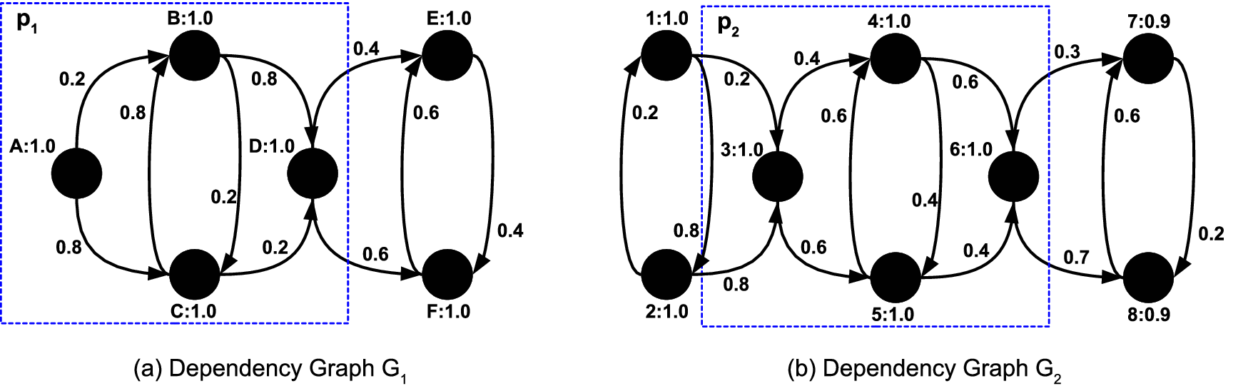
Consider a pattern $p_{1}$= SEQ($A$, AND($B$, $C$), $D$) in Figure 2(a) from [38]. The pattern $p_{1}$ is illustrated as a graph. The vertices of events are $A,B,C,D$. Two edges $BC,CB$ are added due to pattern AND($B$, $C$). According to SEQ($A$, AND($B$, $C$), $D$), both $B$ and $C$ can be performed after $A$ and should be done before $D$. Thus, another 4 edges $AB,AC,BD$ and CD are added. The graph translated from $p_{1}$ is a subgraph of $G_{1}$ surrounded by blue dashed line in Figure 2(a).

For the true mapping $M=\{A\rightarrow 3,B\rightarrow 4,C\rightarrow 5,D\rightarrow 6,E\rightarrow 7,F\rightarrow 8\}$, pattern $p_{1}$ (in $G_{1}$) corresponds to a subgraph $p_{2}$ in $G_{2}$. Since all traces in $\mathcal{L}_{1}$ and $\mathcal{L}_{2}$ match with $p_{1}$ and $p_{2}$, respectively, we have $f_{1}(p_{1})=f_{2}(p_{2})=1.0$. By considering all vertices and edges as patterns in the above Formula, the pattern normal distance of M is $D^{N}(M)=14.91$.

However, the pattern $p_{1}$ has no mapped pattern w.r.t. $M^{\prime}=\{A\rightarrow 6,B\rightarrow 2,C\rightarrow 1,D\rightarrow 3,E\rightarrow 4,F\rightarrow 5\}$. The pattern normal distance of $M^{\prime}$ is 14. While without $p_{1}$, $M^{\prime}$ has a higher score with $D_{v}^{N}(M^{\prime})>D_{v}^{N}(M)$ and $D_{v+e}^{N}(M^{\prime})>D_{v+e}^{N}(M)$. By introducing $p_{1}$, the true mapping M with the highest pattern normal distance beats $M^{\prime}$.

Based on the concept of Petri Net, a firing sequence of a process specification $\mathcal{N}(\mathcal{P},\mathcal{T},\mathcal{F})$, and its post-set, are defined recursively as follows:

1. 1.

   The empty sequence $\epsilon$ is a firing sequence, and $\epsilon\bullet={b_{start}}$;

2. 2.

   If $\sigma$ is a firing sequence, $e\in\mathcal{T}_{s}$ is a transition (event), and $\bullet e\subseteq\sigma\bullet$, then $\sigma e$ is also a firing sequence, and $(\sigma e)\bullet=(\sigma\bullet)-(\bullet e)+(e\bullet)$.

A sequence $\sigma$ is said conforming to a process specification, denoted by $\sigma\models\mathcal{N}_{s}$, if $\sigma$ is a firing sequence w.r.t. $\mathcal{N}_{s}$ and $\sigma\bullet={b_{end}}$.

Let $\sigma$ be a firing sequence. For the next event (transition) $e$, if $\bullet e\not\subseteq\sigma_{k}\bullet$, we call $(\sigma_{k}\bullet,\bullet e)$ a gap with at least one missing event between $\sigma_{k}$ and $e$.

A gap indicates that the previous firing sequence $\sigma$ is successfully executed so far and it is impossible to execute the next event $e$ further. In other words, $\sigma e$ is not a firing sequence. There are some events missing between $\sigma$ and $e$.

For a gap $(\sigma\bullet,\bullet e)$, we call a transition (event) sequence $\tau\in\mathcal{T}^{*}$ a fill of the gap, if it ensures

1. 1.

   $\sigma\tau$ is a firing sequence,

2. 2.

   $\bullet e\subseteq(\sigma\tau)\bullet$.

To recover a sequence $\langle AEF\rangle$ over the process specification in Figure 5, the existing aligning approach enumerates all possible combinations of events in parallel, i.e., $\langle ABCDEF\rangle$, $\langle ABDCEF\rangle$, $\langle ACBD\\ EF\rangle$, $\langle ACDBEF\rangle$, $\langle ADBCEF\rangle$ and $\langle ADCBEF\rangle$. However, any topological sort should always be a minimum recovery, e.g., $\langle ABCDEF\rangle$ with the minimum distance $3$ to the input sequence $\langle AEF\rangle$. There is no need to enumerate other redundant recoveries.

To recover the gap between a firing sequence $\langle A\rangle$ and event $E$, the program generates a set of places $X=\{b_{4},b_{5},b_{6}\}$ in $\bullet E$, but not in $\langle A\rangle\bullet=\{b_{1},b_{2},b_{3}\}$. For each event in $\bullet X=\{B,C,D\}$, e.g., $B$, we fill the gap between the current firing sequence $\langle A\rangle\bullet$ and $\bullet B$. It outputs a firing sequence $\langle AB\rangle$ with post-set $\langle AB\rangle\bullet$ = $\{b_{4},b_{2},b_{3}\}$. Next, by inserting $C\in\bullet X$, we have $\langle ABC\rangle\bullet=\{b_{4},b_{5},b_{3}\}$. It follows $\langle ABCD\rangle\bullet=\{b_{4},b_{5},b_{6}\}$. Finally, the gap between $\langle A\rangle$ and $E$ is filled by $\langle BCD\rangle$ such that $\bullet E\subseteq\langle ABCD\rangle\bullet$.

Consider a sequence $\mathit{x}=\mathit{x}[1],\mathit{x}[2],\dots$, where each $\mathit{x}[i]$ is the value of the $i$-th data point. Each $\mathit{x}[i]$ has a timestamp $\mathit{t}[i]$. For brevity, we write $\mathit{x}[i]$ as $\mathit{x}_{i}$, and $\mathit{t}[i]$ as $\mathit{t}_{i}$.

A speed constraint $\mathit{s}=(\mathit{s}_{\min},\mathit{s}_{\max})$ with window size $\mathit{w}$ is a pair of minimum speed $\mathit{s}_{\min}$ and maximum speed $\mathit{s}_{\max}$ over the sequence $\mathit{x}$. We say that a sequence $\mathit{x}$ satisfies the speed constraint $\mathit{s}$, denoted by $\mathit{x}\vDash\mathit{s}$, if for any $\mathit{x}_{i},\mathit{x}_{j}$ in a window, i.e., $0<\mathit{t}_{j}-\mathit{t}_{i}\leq\mathit{w}$, it has $\mathit{s}_{\min}\leq\frac{\mathit{x}_{j}-\mathit{x}_{i}}{\mathit{t}_{j}-\mathit{t}_{i}}\leq\mathit{s}_{\max}.$

The window $w$ denotes a period of time. In real settings, speed constraints are often meaningful within a certain period. For example, it is reasonable to consider the maximum walking speed in hours (rather than the speed between two arbitrary observations in different years), since a person usually cannot keep on walking in his/her maximum speed for several years without a break. In other words, it is sufficient to validate the speed w.r.t. two points $\mathit{x}_{i},\mathit{x}_{j}$ in a window $w=24$ hours, i.e., whether $\mathit{s}_{\min}\leq\frac{\mathit{x}_{j}-\mathit{x}_{i}}{\mathit{t}_{j}-\mathit{t}_{i}}\leq\mathit{s}_{\max},0<\mathit{t}_{j}-\mathit{t}_{i}\leq\mathit{w}$. In contrast, considering the speed w.r.t. two points in an extremely large period (e.g., two observation points in different years) is meaningless and unnecessary. Similar examples include the speed constraints on stock price whose daily limit is directly determined by the price of the last trading day, i.e., with window size 1.

The speed constraint $\mathit{s}$ can be either positive (restricting value increase) or negative (on decrease). In most scenarios, the speed constraint is natural, e.g., the fuel consumption of a crane should not be negative and not exceed 40 liters per hour, while some others could be derived.

A repair $\mathit{x}^{\prime}$ of $\mathit{x}$ is a modification of the values $\mathit{x}_{i}$ to $\mathit{x}^{\prime}_{i}$ where $\mathit{t}^{\prime}_{i}=\mathit{t}_{i}$. Referring to the minimum change principle in data repairing [3], the repair distance is evaluated by the difference between the original $\mathit{x}$ and the repaired $\mathit{x}^{\prime}$,

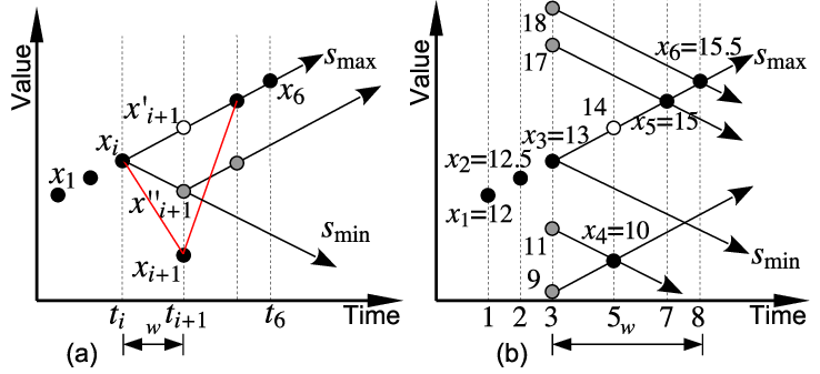
Consider a sequence $\mathit{x}=\{12,12.5,13,10,15,15.5\}$ of six data points, with timestamps $\mathit{t}=\{1,2,3,5,7,8\}$. Figure 6(a) from [40] illustrates the data points (in black). Suppose that the speed constraints are $\mathit{s}_{\max}=0.5$ and $\mathit{s}_{\min}=-0.5$.

For a window size $\mathit{w}=2$ in the speed constraints, data points $\mathit{x}_{3}$ and $\mathit{x}_{4}$, with timestamp distance $5-3\leq 2$ in a window, are identified as violations to $\mathit{s}_{\min}=-0.5$, since the speed is $\frac{10-13}{5-3}=-1.5<-0.5$. Similarly, $\mathit{x}_{4}$ and $\mathit{x}_{5}$ with speed $\frac{15-10}{7-5}=2.5>0.5$ are violations to $\mathit{s}_{\max}=0.5$.

To remedy the violations (denoted by red lines), a repair on $\mathit{x}_{4}$ can be performed, i.e., $\mathit{x}^{\prime}_{4}=14$ (the white data point). As illustrated in Figure 6(a), the repaired sequence satisfies both the maximum and minimum speed constraints. The repair distance is $\Delta(\mathit{x},\mathit{x}^{\prime})=|10-14|=4$.

Note that if the window size is too small such as $\mathit{w}=1$, the violations between $\mathit{x}_{3}$ and $\mathit{x}_{4}$ (as well as $\mathit{x}_{4}$ and $\mathit{x}_{5}$) could not be detected, since their timestamp distance is $2>1$. On the other hand, if the window size is too large, say $\mathit{w}=10$, then all the pairs of data points in $\mathit{x}$ have to be compared. Although the same repair $\mathit{x}^{\prime}$ is obtained, the computation overhead is obviously higher (and unnecessary). Song et al. [40] also propose to determine an adaptive window size for balancing accuracy and efficiency.

Two labels $l_{1},l_{2}$ match a constraint graph $\mathcal{S}(L,N)$, denoted by $(l_{1},l_{2})\asymp\mathcal{S}$, if either $l_{1}=l_{2}$ denotes the same label or $(l_{1},l_{2})\in N$ is an edge in $\mathcal{S}$. For example, in Figure 7(a), we have $(a,a)\asymp\mathcal{S},(a,b)\asymp\mathcal{S}$, but $(a,d)\not\asymp\mathcal{S}$. It is worth noting that $(a,a)\asymp\mathcal{S}$ implies the self-loop relationship of labels in S.

An instance graph $G(V,E)$ satisfies a constraint graph $\mathcal{S}(L,N)$, denoted by $G\models S$, if $(v,u)\in E$ implies $(\lambda(v),\lambda(u))\asymp\mathcal{S},\forall(v,u)\in E$. That is, for any edge $(v,u)\in E$, their labels $\lambda(v),\lambda(u)$ must match the constraint graph $\mathcal{S}$ with either $\lambda(v)=\lambda(u)$ or $(\lambda(v),\lambda(u))\in N$.

We call $(v,u)$ a violation to the constraint graph $\mathcal{S}$, if $(v,u)\in E$ and $(\lambda(v),\lambda(u))\not\asymp S$. For example, in Figure 7(b), the edge $(1,3)$ indicates a violation to $\mathcal{S}$, as their labels $(a,d)\not\asymp S$ are neither the same nor adjacent in Figure 7(a) of constraints.

Consider the example in Figure 8 with relabeling cost $\delta(c,g)=\delta(f,d)=1$. When conducting a greedy method, the best choice may be repairing vertex $6$ with label $d$. The violation between vertexes $5$ and $6$ is eliminated, and there is no new violation among vertexes introduced after relabeling vertex $6$ to $d$. The relabeling steps terminate with all the neighborhood constraints satisfied.

A causal net is a Petri net $N=(P,T,F)$ such that for every $p\in P$, $|pre_{F}(p)|\leq 1$ and $|post_{F}(p)|\\ \leq 1$.

It is easy to see that there will be no XOR-split or XOR-join in a causal net (according to the maximum in/out degree 1 of places), while AND-split and AND-join are allowed. If we interpret places as edges connecting two transitions, the net is indeed a directed acyclic graph of transitions.

An execution of a process specification $N_{s}(P_{s},T_{s},F_{s})$ is denoted by $(N_{\sigma},\pi)$, where $N_{\sigma}(P_{\sigma},T_{\sigma},F_{\sigma})$ is a causal net and $\pi$ is a labeling $\pi:P_{\sigma}\cup T_{\sigma}\rightarrow P_{s}\cup T_{s}$ such that $\pi(P_{\sigma})\subseteq P_{s}$, and $\pi(T_{\sigma})\subseteq T_{s}$.

We say an execution $(N_{\sigma},\pi)$ conforms to a process specification $N_{s}$, denoted by $(N_{\sigma},\pi)\models N_{s}$, if and only if (i) $\pi(P_{\sigma})\subseteq P_{s}$ and $\pi(T_{\sigma})\subseteq T_{s}$; (ii) for any $t\in T_{\sigma}$, $\pi(pre_{F_{\sigma}}(t))=pre_{F_{s}}(\pi(t))$ and $\pi(post_{F_{\sigma}}(t))=post_{F_{s}}(\pi(t))$; (iii) for any $p\subseteq P_{\sigma}$, $pre_{F_{\sigma}}(p)=\emptyset$ implies $pi(p)$ = start and $post_{F_{\sigma}}(p)=\emptyset$ indicates $\pi(p)$ = end.

Consider the execution trace in Figure 9(b) over the specification in Figure 9(a) from [44]. We represent the corresponding causal net in Figure 9(c) as follows. For the first $t_{1}$ without any prerequisite, we put a place $p_{0}$ with $\pi(p_{0})$ = start as the $pre$ set. The second $\sigma(2)$ of $t_{2}$ has prerequisite $pre_{F_{\sigma}}(pre_{F_{\sigma}}(t_{2}))={t_{1}}$. We recover the labeling of the place $p_{1}$ between $t_{2}$ and its prerequisite $t_{1}$ to the place between $\pi(t_{2})$ and $\pi(t_{1})$ in the specification, i.e., $\pi(p_{1})=a$. Similarly, considering the prerequisites of $t_{5}$, $pre_{F_{\sigma}}(pre_{F_{\sigma}}(t_{5}))={t_{3},t_{4}}$, we obtain $\pi(p_{3})=c,\pi(p_{5})=e$. For the last $t_{6}$, which is not prerequisite of any others, a place $p_{7}$ : end is appended as $post_{F_{\sigma}}(t_{6})$.

Referring to conformance definition, for any transition, say $t_{1}$ for instance, we have $\pi(pre_{F_{\sigma}}(t_{1}))=\pi(p_{0})={start}=pre_{F_{s}}(submit)=pre_{F_{s}}(\pi(t_{1}))$ and $\pi(post_{F_{\sigma}}(t_{2}))=\pi({p_{2},p_{4}})={b,d}=post_{F_{s}}(design)=post_{F_{s}}(\pi(t_{2}))$.

References

- [1] A. Adriansyah, B. F. van Dongen, and N. Zannone. Controlling break-the-glass through alignment. In International Conference on Social Computing, SocialCom 2013, Washington, DC, USA, 8-14 September, 2013, pages 606–611. IEEE, 2013.
- [2] E. Alevizos, A. Skarlatidis, A. Artikis, and G. Paliouras. Probabilistic complex event recognition: A survey. ACM Comput. Surv., 50(5):71:1–71:31, 2017.
- [3] P. Bohannon, M. Flaster, W. Fan, and R. Rastogi. A cost-based model and effective heuristic for repairing constraints by value modification. In Proceedings of the ACM SIGMOD International Conference on Management of Data, Baltimore, Maryland, USA, June 14-16, 2005, pages 143–154, 2005.
- [4] F. Casati, M. Castellanos, N. Salazar, and U. Dayal. Abstract process data warehousing. In R. Chirkova, A. Dogac, M. T. Özsu, and T. K. Sellis, editors, Proceedings of the 23rd International Conference on Data Engineering, ICDE 2007, The Marmara Hotel, Istanbul, Turkey, April 15-20, 2007, pages 1387–1389. IEEE, 2007.
- [5] T. Dasu, R. Duan, and D. Srivastava. Data quality for temporal streams. IEEE Data Eng. Bull., 39(2):78–92, 2016.
- [6] M. de Leoni, F. M. Maggi, and W. M. P. van der Aalst. Aligning event logs and declarative process models for conformance checking. In Business Process Management - 10th International Conference, BPM 2012, Tallinn, Estonia, September 3-6, 2012. Proceedings, volume 7481 of Lecture Notes in Computer Science, pages 82–97. Springer, 2012.
- [7] M. de Leoni, F. M. Maggi, and W. M. P. van der Aalst. An alignment-based framework to check the conformance of declarative process models and to preprocess event-log data. Inf. Syst., 47:258–277, 2015.
- [8] R. Dechter, I. Meiri, and J. Pearl. Temporal constraint networks. Artif. Intell., 49(1-3):61–95, 1991.
- [9] R. M. Dijkman, M. Dumas, and L. García-Bañuelos. Graph matching algorithms for business process model similarity search. In Business Process Management, 7th International Conference, BPM 2009, Ulm, Germany, September 8-10, 2009. Proceedings, pages 48–63, 2009.
- [10] L. Ding, S. Chen, E. A. Rundensteiner, J. Tatemura, W. Hsiung, and K. S. Candan. Runtime semantic query optimization for event stream processing. In Proceedings of the 24th International Conference on Data Engineering, ICDE 2008, April 7-12, 2008, Cancún, México, pages 676–685. IEEE, 2008.
- [11] Z. Dong, L. Wen, H. Huang, and J. Wang. CFS: A behavioral similarity algorithm for process models based on complete firing sequences. In On the Move to Meaningful Internet Systems: OTM 2014 Conferences - Confederated International Conferences: CoopIS, and ODBASE 2014, Amantea, Italy, October 27-31, 2014, Proceedings, volume 8841 of Lecture Notes in Computer Science, pages 202–219. Springer, 2014.
- [12] D. R. Ferreira and D. Gillblad. Discovering process models from unlabelled event logs. In Business Process Management, 7th International Conference, BPM 2009, Ulm, Germany, September 8-10, 2009. Proceedings, pages 143–158, 2009.
- [13] Y. Gao, S. Song, X. Zhu, J. Wang, X. Lian, and L. Zou. Matching heterogeneous event data. IEEE Trans. Knowl. Data Eng., 30(11):2157–2170, 2018.
- [14] L. Golab, H. J. Karloff, F. Korn, A. Saha, and D. Srivastava. Sequential dependencies. PVLDB, 2(1):574–585, 2009.
- [15] R. Huang. Approximate event pattern matching over heterogeneous and dirty sources. In M. d’Aquin, S. Dietze, C. Hauff, E. Curry, and P. Cudré-Mauroux, editors, CIKM ’20: The 29th ACM International Conference on Information and Knowledge Management, Virtual Event, Ireland, October 19-23, 2020, pages 3237–3240. ACM, 2020.
- [16] S. R. Jeffery, G. Alonso, M. J. Franklin, W. Hong, and J. Widom. Declarative support for sensor data cleaning. In Pervasive Computing, 4th International Conference, PERVASIVE 2006, Dublin, Ireland, May 7-10, 2006, Proceedings, pages 83–100, 2006.
- [17] G. Jeh and J. Widom. Simrank: a measure of structural-context similarity. In Proceedings of the Eighth ACM SIGKDD International Conference on Knowledge Discovery and Data Mining, July 23-26, 2002, Edmonton, Alberta, Canada, pages 538–543, 2002.
- [18] T. Jin, J. Wang, and L. Wen. Efficient retrieval of similar workflow models based on behavior. In Web Technologies and Applications - 14th Asia-Pacific Web Conference, APWeb 2012, Kunming, China, April 11-13, 2012. Proceedings, volume 7235 of Lecture Notes in Computer Science, pages 677–684. Springer, 2012.
- [19] J. Kang and J. F. Naughton. On schema matching with opaque column names and data values. In Proceedings of the 2003 ACM SIGMOD International Conference on Management of Data, San Diego, California, USA, June 9-12, 2003, pages 205–216, 2003.
- [20] Y. Kobayashi, A. Kishimoto, and O. Watanabe. Evaluations of hash distributed a* in optimal sequence alignment. In T. Walsh, editor, IJCAI 2011, Proceedings of the 22nd International Joint Conference on Artificial Intelligence, Barcelona, Catalonia, Spain, July 16-22, 2011, pages 584–590. IJCAI/AAAI, 2011.
- [21] A. Langley. Strategies for theorizing from process data. Academy of Management review, 24(4):691–710, 1999.
- [22] X. Li, X. L. Dong, K. Lyons, W. Meng, and D. Srivastava. Truth finding on the deep web: Is the problem solved? PVLDB, 6(2):97–108, 2012.
- [23] Z. Li and T. Ge. PIE: approximate interleaving event matching over sequences. In 31st IEEE International Conference on Data Engineering, ICDE 2015, Seoul, South Korea, April 13-17, 2015, pages 747–758. IEEE Computer Society, 2015.
- [24] X. Lian, L. Chen, and S. Song. Consistent query answers in inconsistent probabilistic databases. In Proceedings of the ACM SIGMOD International Conference on Management of Data, SIGMOD 2010, Indianapolis, Indiana, USA, June 6-10, 2010, pages 303–314, 2010.
- [25] A. Margara, G. Cugola, and G. Tamburrelli. Learning from the past: automated rule generation for complex event processing. In The 8th ACM DEBS 2014, pages 47–58, 2014.
- [26] S. Melnik, H. Garcia-Molina, and E. Rahm. Similarity flooding: A versatile graph matching algorithm and its application to schema matching. In Proceedings of the 18th International Conference on Data Engineering, San Jose, CA, USA, February 26 - March 1, 2002, pages 117–128, 2002.
- [27] T. Murata. Petri nets: Properties, analysis and applications. Proceedings of the IEEE, 77(4):541–580, Apr 1989.
- [28] G. Navarro. A guided tour to approximate string matching. ACM Comput. Surv., 33(1):31–88, 2001.
- [29] S. Nejati, M. Sabetzadeh, M. Chechik, S. M. Easterbrook, and P. Zave. Matching and merging of statecharts specifications. In 29th International Conference on Software Engineering (ICSE 2007), Minneapolis, MN, USA, May 20-26, 2007, pages 54–64, 2007.
- [30] T. Pedersen, S. Patwardhan, and J. Michelizzi. Wordnet: : Similarity - measuring the relatedness of concepts. In Proceedings of the Nineteenth National Conference on Artificial Intelligence, Sixteenth Conference on Innovative Applications of Artificial Intelligence, July 25-29, 2004, San Jose, California, USA, pages 1024–1025, 2004.
- [31] A. Rozinat and W. M. P. van der Aalst. Conformance checking of processes based on monitoring real behavior. Inf. Syst., 33(1):64–95, 2008.
- [32] S. Song, Y. Cao, and J. Wang. Cleaning timestamps with temporal constraints. PVLDB, 9(10):708–719, 2016.
- [33] S. Song and L. Chen. Discovering matching dependencies. In Proceedings of the 18th ACM Conference on Information and Knowledge Management, CIKM 2009, Hong Kong, China, November 2-6, 2009, pages 1421–1424, 2009.
- [34] S. Song and L. Chen. Differential dependencies: Reasoning and discovery. ACM Trans. Database Syst., 36(3):16, 2011.
- [35] S. Song, L. Chen, and H. Cheng. Efficient determination of distance thresholds for differential dependencies. IEEE Trans. Knowl. Data Eng., 26(9):2179–2192, 2014.
- [36] S. Song, L. Chen, and P. S. Yu. Comparable dependencies over heterogeneous data. VLDB J., 22(2):253–274, 2013.
- [37] S. Song, H. Cheng, J. X. Yu, and L. Chen. Repairing vertex labels under neighborhood constraints. PVLDB, 7(11):987–998, 2014.
- [38] S. Song, Y. Gao, C. Wang, X. Zhu, J. Wang, and P. S. Yu. Matching heterogeneous events with patterns. IEEE Trans. Knowl. Data Eng., 29(8):1695–1708, 2017.
- [39] S. Song, C. Li, and X. Zhang. Turn waste into wealth: On simultaneous clustering and cleaning over dirty data. In L. Cao, C. Zhang, T. Joachims, G. I. Webb, D. D. Margineantu, and G. Williams, editors, Proceedings of the 21th ACM SIGKDD International Conference on Knowledge Discovery and Data Mining, Sydney, NSW, Australia, August 10-13, 2015, pages 1115–1124. ACM, 2015.
- [40] S. Song, A. Zhang, J. Wang, and P. S. Yu. SCREEN: stream data cleaning under speed constraints. In Proceedings of the 2015 ACM SIGMOD International Conference on Management of Data, Melbourne, Victoria, Australia, May 31 - June 4, 2015, pages 827–841. ACM, 2015.
- [41] S. Song, H. Zhu, and L. Chen. Probabilistic correlation-based similarity measure on text records. Inf. Sci., 289:8–24, 2014.
- [42] P. Sun, Z. Liu, S. B. Davidson, and Y. Chen. Detecting and resolving unsound workflow views for correct provenance analysis. In Proceedings of the ACM SIGMOD International Conference on Management of Data, SIGMOD 2009, Providence, Rhode Island, USA, June 29 - July 2, 2009, pages 549–562. ACM, 2009.
- [43] W. M. P. van der Aalst et al. Process mining manifesto. In Business Process Management Workshops - BPM 2011 International Workshops, Part I, volume 99 of Lecture Notes in Business Information Processing, pages 169–194. Springer, 2011.
- [44] J. Wang, S. Song, X. Lin, X. Zhu, and J. Pei. Cleaning structured event logs: A graph repair approach. In 31st IEEE International Conference on Data Engineering, ICDE 2015, Seoul, South Korea, April 13-17, 2015, pages 30–41, 2015.
- [45] J. Wang, S. Song, X. Zhu, and X. Lin. Efficient recovery of missing events. PVLDB, 6(10):841–852, 2013.
- [46] J. Wang, S. Song, X. Zhu, X. Lin, and J. Sun. Efficient recovery of missing events. IEEE Trans. Knowl. Data Eng., 28(11):2943–2957, 2016.
- [47] Y. Wang, S. Song, L. Chen, J. X. Yu, and H. Cheng. Discovering conditional matching rules. TKDD, 11(4):46:1–46:38, 2017.
- [48] M. Weidlich, R. M. Dijkman, and J. Mendling. The icop framework: Identification of correspondences between process models. In Advanced Information Systems Engineering, 22nd International Conference, CAiSE 2010, Hammamet, Tunisia, June 7-9, 2010. Proceedings, pages 483–498, 2010.
- [49] E. Wu, Y. Diao, and S. Rizvi. High-performance complex event processing over streams. In S. Chaudhuri, V. Hristidis, and N. Polyzotis, editors, Proceedings of the ACM SIGMOD International Conference on Management of Data, Chicago, Illinois, USA, June 27-29, 2006, pages 407–418. ACM, 2006.
- [50] A. Zhang, S. Song, and J. Wang. Sequential data cleaning: A statistical approach. In Proceedings of the 2016 International Conference on Management of Data, SIGMOD Conference 2016, San Francisco, CA, USA, June 26 - July 01, 2016, pages 909–924, 2016.
- [51] H. Zhang, Y. Diao, and N. Immerman. Recognizing patterns in streams with imprecise timestamps. PVLDB, 3(1):244–255, 2010.
- [52] J. J. Zhang, R. H. Y. Chan, and P. Fung. Extractive speech summarization using shallow rhetorical structure modeling. IEEE Trans. Audio, Speech & Language Processing, 18(6):1147–1157, 2010.
- [53] J. J. Zhang and P. Fung. Active learning with semi-automatic annotation for extractive speech summarization. TSLP, 8(4):6:1–6:25, 2012.
- [54] J. J. Zhang and P. Fung. Automatic parliamentary meeting minute generation using rhetorical structure modeling. IEEE Trans. Audio, Speech & Language Processing, 20(9):2492–2504, 2012.
- [55] X. Zhu, S. Song, X. Lian, J. Wang, and L. Zou. Matching heterogeneous event data. In International Conference on Management of Data, SIGMOD 2014, Snowbird, UT, USA, June 22-27, 2014, pages 1211–1222, 2014.
- [56] X. Zhu, S. Song, J. Wang, P. S. Yu, and J. Sun. Matching heterogeneous events with patterns. In IEEE 30th International Conference on Data Engineering, Chicago, ICDE 2014, IL, USA, March 31 - April 4, 2014, pages 376–387, 2014.