Location-aware Single Image Reflection Removal
Abstract
This paper proposes a novel location-aware deep-learning-based single image reflection removal method. Our network has a reflection detection module to regress a probabilistic reflection confidence map, taking multi-scale Laplacian features as inputs. This probabilistic map tells if a region is reflection-dominated or transmission-dominated, and it is used as a cue for the network to control the feature flow when predicting the reflection and transmission layers. We design our network as a recurrent network to progressively refine reflection removal results at each iteration. The novelty is that we leverage Laplacian kernel parameters to emphasize the boundaries of strong reflections. It is beneficial to strong reflection detection and substantially improves the quality of reflection removal results. Extensive experiments verify the superior performance of the proposed method over state-of-the-art approaches. Our code and the pre-trained model can be found at https://github.com/zdlarr/Location-aware-SIRR.
1 Introduction
Reflections often occur when images are photographed through reflective and transparent media (e.g., glass). Removing undesired reflections enhances the image quality and benefits many follow-up computer vision tasks, such as image classification. In reflection removal, an image with reflections can be modeled as the weighted additive composition of a transmission layer and a reflection layer . Precisely, following the alpha blending model in [4, 23, 57], we express the composition procedure as:
| (1) |
where here is an alpha blending mask and indicates the element-wise multiplication. This model is designed to approximate the complex physical mechanisms involved in forming images with reflections.
 |
 |
 |
| (a) Input | (b) Zhang et al. [57] | (c) RMNet [47] |
 |
 |
 |
| (d) ERRNet [46] | (e) CoRRN [44] | (f) IBCLN [23] |
 |
 |
 |
| (g) RCMap | (h) Ours | (i) Ground truth |
The task of single image reflection removal (SIRR) is to recover from a given image . It is an ill-posed problem since the number of unknowns is much more than the number of equations derived from Eq. 1. Therefore, priors are necessary to constrain the solution space, such as natural image gradient sparsity [21, 22], ghosting cues for thick glasses [34], and relative smoothness that assumes the refection layer is smoother than the transmission layer [24, 52]. To disambiguate the restoration of and in the gradient domain, several works propose first to determine the locations of reflection-dominated and transmission-dominated pixels, and then exploit different constraints at different locations to improve the reflection removal results [21, 40, 42]. While these methods are sensitive to the selection of hyperparameters, for instance, the commonly used gradient magnitude threshold, the detected location information is proven to be useful to handle strong reflections. Therefore, such location information is expected to be beneficial for the neural networks to learn how the reflection information is encoded in the features. However, it is rarely investigated in deep learning-based SIRR methods [4, 15, 18, 23, 46, 47, 50, 57]. This might cause ambiguities when strong reflections appear. We observe that state-of-the-art SIRR methods typically fail to recover high-quality transmission layers in such cases.
This paper proposes a location-aware deep learning-based SIRR method for generic reflection removal. Our network incorporates a novel reflection detection module (RDM) to detect reflection-dominated regions via learning multi-scale Laplacian features. The output of RDM is a probabilistic reflection confidence map (RCMap), which controls the subsequent feature flow, resulting in significantly improved SIRR results. Although this detection-and-removal strategy has been explored in shadow analysis [3, 12, 13, 16, 31, 45] and rain removal [6, 17, 30, 51, 54, 55] tasks, they mainly exploit features learned in the RGB domain, which are different from our approach in two aspects. First, motivated by the relative smoothness prior in [24], which assumes that the characteristics of and in the gradient domain are different, we use the learned Laplacian kernel to emphasize the boundaries of strong reflections and suppress low-frequency reflections, which is beneficial to improve the quality of RCMaps. Second, RDM is trained without ground-truth reflection-dominated region masks. This can avoid the difficulty of defining or labeling reflection-dominated regions. The inverse RCMap, i.e., 1 - RCMap, can serve as the weight map in Eq. 1 and be used to indicate the transmission-dominated regions. It motivates us to use Eq. 1 as a loss to control the RDM training.
Our proposed network iteratively restores the transmission layer from the corrupted input. In each iteration, we formulate the restoration process in a removal-by-detection manner. It first detects the reflection-dominated regions based on the RCMap and then predicts the whole reflection layer by suppressing the transmission information. Afterwards, it restores the transmission layer by jointly leveraging the transmission-dominant regions and the predicted reflection layer. Such a network design decomposes the complicated SIRR problem into sub-problems and considers the mutual dependence between reflection and transmission. As illustrated in Fig. 1, our network can effectively remove strong reflected highlights.
In summary, the main contributions of our work are:
- •
We propose a novel SIRR method that iteratively restores the transmission layer from the corrupted input image. At each iteration, the restoration process is formulated in a removal-by-detection sequential manner.
- •
We propose a novel reflection detection module (RDM) to locate the reflection-dominated regions. It learns a group of multi-scale Laplacian kernel parameters to exploit reflection boundary information.
- •
Extensive experiments show that the proposed location-aware neural network outperforms state-of-the-art SIRR methods in removing strong reflections.
2 Related Work
A variety of reflection removal methods, such as multi-view or video-based [5, 8, 25, 26, 27, 33, 37, 38, 39, 49], dual-pixel sensor-based [29] and polarization-based [2, 20, 35] methods, have been proposed to restore the transmission layer through motion or optical cues. Since we focus on SIRR in this paper, we mainly review the single image based methods below.
To handle the ill-posed SIRR problem, traditional optimization-based methods introduce different priors [21, 22]. Observing that reflection layers are usually out of focus and appear to be more blurry than transmission layers, Li et al. [24] introduced a relative smoothness prior to distinguish the gradients of the two layers with different probability distributions. Shih et al. [34] exploited ghosting cues to remove reflections when the thickness of the glass cannot be ignored. Huang et al. [14] proposed a wavelet transform based regularization method to separate ghosting patterns from background patterns. Multi-scale depth-of-field (DoF) analysis based methods [40, 42] were proposed to separate reflection from transmissions by detecting the reflection-dominated regions. However, the thresholds in these methods for determining the reflection regions are vulnerable to noise. In [1, 52], the Laplacian data fidelity term is used to suppress the blurry reflections. However, these two methods cannot effectively remove strong reflections and might smooth out the transmission layer’s details. In contrast, we leverage Laplacian features to emphasize the boundaries of strong reflections as a clue for the network to remove them.
Recently, many deep-learning-based methods [4, 15, 18, 23, 46, 47, 50, 56, 57] were proposed to solve the SIRR problem by learning task-specific features. Fan et al. [4] designed a deep neural network, called CEIL-Net, to first regress the edge map of the transmission layer and then reconstruct the transmission layer. Yang et al. [50] proposed the BDN, a multi-stage network for estimating two layers sequentially, where the reflection layer predicted in the previous stage is used as auxiliary information to guide the transmission layer reconstruction in the next stage. Li et al. [23] proposed the IBCLN method, which is an LSTM based recurrent network for concurrently refining the results of the predicted reflection and transmission layers. Wan et al. [44] proposed a feature-sharing strategy and a statistical loss for removing the strong reflections within local regions. They further proposed to study the face reflection removal problem in [43]. Zhang et al. [56] proposed to explore the edge hints in the user-specified regions to separate the reflection and transmission layers. Some methods proposed to generate more representative training data. Jin et al. [15] proposed multiple data generation models. Wen et al. [47] proposed SynNet to generate images with reflections beyond linearity. Wei et al. [46] introduced an alignment-invariant loss to utilize the misaligned images as the real-world training dataset. Kim et al. [18] proposed a physics-based rendering method to render realistic images with reflections. Unlike these methods, this paper explores how to incorporate the location information of reflections into the network for controlling the feature flow.
Many loss terms were used to boost the SIRR performance [18, 23, 46, 47, 50, 57], e.g., the VGG-based perceptual loss, exclusion loss in the gradient domain, and adversarial loss to prevent the blurring effects. In this paper, a new composition loss without using the GT reflection-dominated region masks is proposed to train our RDM.
3 Method

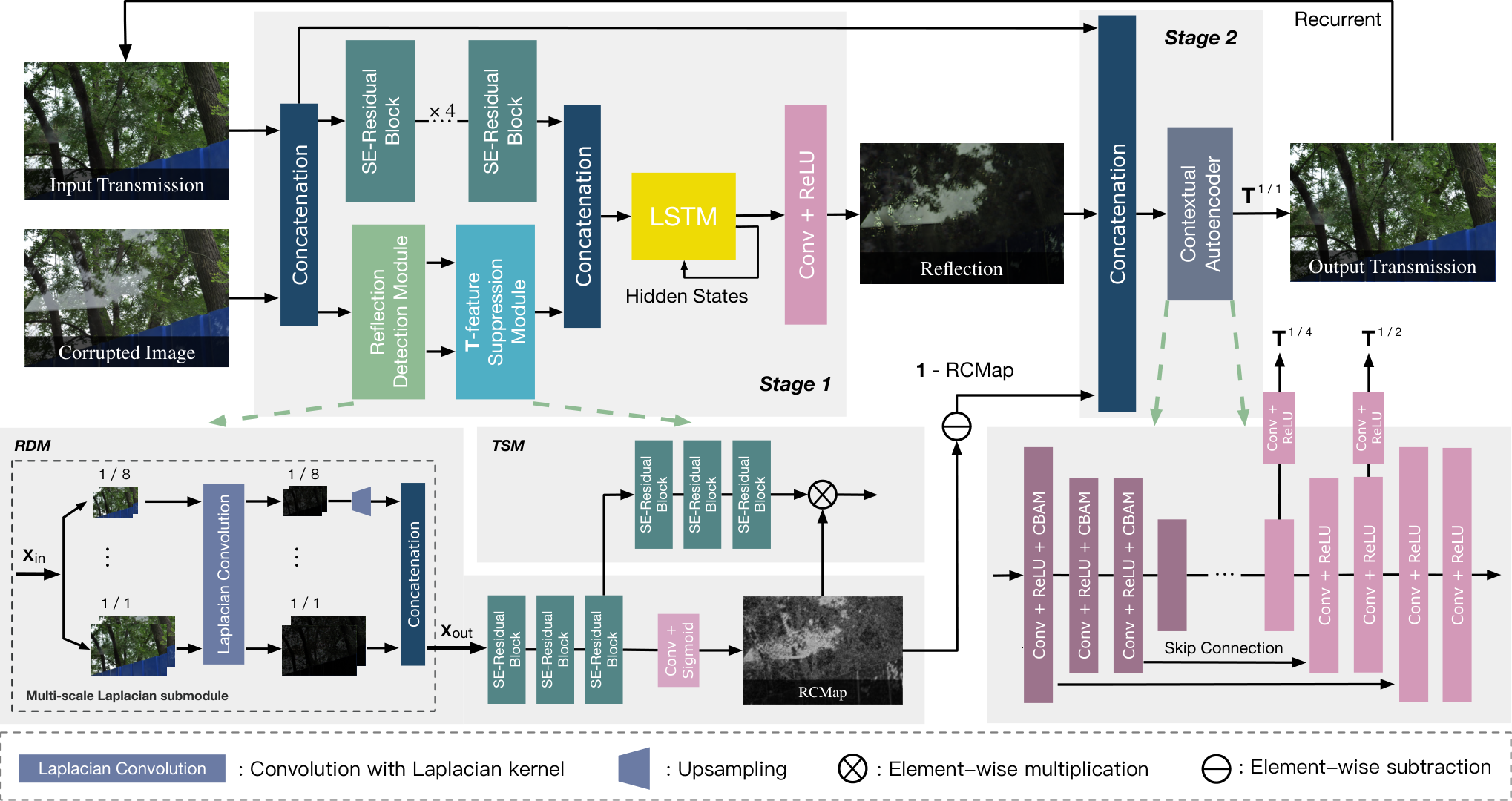
Our network is a recurrent network, as illustrated in Fig. 2. In each iteration , our network takes the original image and the transmission layer predicted in the previous iteration as inputs, and predicts the transmission layer to continue the iteration. is initialized as . The recurrent structure of our network is inspired by IBCLN [23]. However, different from jointly estimating the transmission and reflection layers in IBCLN, we design our model to reconstruct the transmission layer conditioned on the RCMap and the restored reflection layer at each iteration. The step-by-step refinement results of reflection removal are shown in Fig. 3.
Like BDN [50], each iteration of our network is divided into two stages to restore two layers sequentially. However, we leverage RCMap to control the between-stage information flow. In the first stage, we predict the reflection layer and RCMap by taking and as inputs. We denote the first stage as the function :
| (2) |
This stage mainly consists of two modules: the reflection detection module (RDM) and the transmission-feature suppression module (TSM). Specifically, The RDM takes and as inputs and predicts the confidence map using features from a multi-scale Laplacian sub-module (MLSM). Next, the TSM is used to suppress the Laplacian features within transmission-dominated regions via an element-wise multiplication between the features and . Afterwards, the suppressed features and the image features are concatenated as the inputs of an LSTM [10] block to estimate . In our work, and are mainly used as cues to facilitate the reconstruction of transmission layers.
In the second stage, we predict the transmission layer with the input of as well as computed in the first stage. We denote the second stage as a function which can be described as:
| (3) |
Notice that we utilize the inverse confidence map, i.e. , in this stage. Since the transmission layer dominates at regions where have a high value, we expect this map to help the network learn weights to encode the reflection information in an adaptive manner, which should benefit the reconstruction of the transmission layer. For the network structure in this stage, we follow the contextual auto-encoder network in [30], and additionally leverage CBAM (Convolutional Block Attention Module) [48] blocks after Conv and ReLU to compute the channel-wise and spatial attention. Please refer to Sec.1 in the supplemental material for detailed network architecture.

Multi-scale Laplacian Features. We observe that the Laplacian operator, a second-order differential operator, can suppress the low-frequency reflections better. As illustrated in Fig. 4, low-frequency reflections are less evident in the inverse Laplacian map than in the inverse edge map, which suggests that the Laplacian operator suppresses low-frequency reflections more effectively. In contrast, strong reflections that have hard boundaries can not be suppressed by the Laplacian operator. It is possible that the difference between and caused by strong reflections becomes more obvious in the Laplacian domain. We assume such a behavior of the Laplacian operator is beneficial to detect reflection-dominated regions and thus concatenate these two images to form as inputs to obtain multi-scale Laplacian features.

For the purpose of multi-scale Laplacian feature learning, we down-sample through scaling the height and width of input images using bi-linear interpolation with the following factors: 1/2, 1/4, 1/8 [7]. The down-sampled results are denoted by respectively. We utilize a convolution kernel with weights initialized to be a Laplacian kernel, denoted by , to obtain the second derivative signal from . We allow the network to fine-tune the Laplacian kernel parameters to better extract Laplacian features, where the fine-tuned parameters are denoted as . During training, we utilize gradient clipping (0.25 in our experiments) to make sure that the learned kernel stays close to the original kernel .
After the Laplacian convolution block in Fig. 2, the up-sampling operation is applied to the multi-scale Laplacian feature maps to restore their original size, where is the sampling rate. Precisely, given the images and , the output features can be written as:
| (4) |
where is the concatenation operation.
Finally, taking as input, RDM predicts the reflection confidence map from the Laplacian features. We employ three Squeeze-and-Excitation Residual Block (SE-ResBlocks) [11] to get efficient multi-channel Laplacian features, where each block comprises of three layers of SE-ResNet, then the PReLU function [9] is used to activate the features while keeping the negative values. These combined blocks denotes as . Thus, given the features , the map can be described as:
| (5) |
The improvement of the predicted RCMaps for two synthesized images along with iterations is illustrated in Fig. 5.
Transmission-feature suppression module. In this module, we employ three SE-ResBlocks to refine the Laplacian features and then multiply the features by for the purpose of transmission features suppressing. Instead of predicting with RCMap as input, just like predicting in the second stage, we empirically found that suppressing the part of Laplacian features belong to transmission-dominated regions benefits the reflection layer prediction. It also leads to a relatively simple network design by concatenating the features computed with and the suppressed Laplacian features as the input to the LSTM [10] block. That is, the same encoder-decoder network structure in the second stage is not used in the first stage to reduce the number of network parameters.
4 Training Loss
In this section, we describe the four loss functions used in the training of our network. For clarity, we denote the ground-truth transmission and reflection layers by , the predicted transmission and reflection layers at iteration as respectively, and inverse gamma correction as a function . The iterations number used in our recurrent network is denoted by .
Composition Loss. The composition loss is proposed to guide the training of RDM for predicting and supervise , at each iteration using training images synthesized by the following linear alpha blending model in [57]:
| (6) |
where is a scalar, and .
Firstly, since the map can serve as the weight map in Eq. 1, we can compose an image by the following formula using gamma corrected and :
| (7) |
where is an element-wise production operation. We formulate the loss for RCMap as follows:
| (8) |
where indicates the mean squared error, is an attenuation coefficient to indicate the strength of supervision and we set it to 0.85.
Secondly, same as IBCLN [23], we adopt Eq. 6 to form a residual loss to guide the prediction of in two forms: and , where is a known scalar used to synthesize training images. We use Eq. 8 to compute the difference between and , and denote the loss as . The composition loss for the synthesized images is defined as:
| (9) |
Perceptual Loss. We use VGG-19 network [36] pre-trained on ImageNet [32] dataset to extract features for the computation of our perceptual loss. This loss takes multi-scale images as inputs and can be written into:
| (10) |
where denotes the loss between VGG features. indicates the output of the last layer of the autoencoder in stage 2 at iteration N, and indicates the ground truth that has the same scale as . We set respectively. For , we use the layers ‘conv_2’ () of the standard VGG-19 net. Fig. 2 shows how the network computes .
Pixel and SSIM Loss. The pixel loss is used to penalize the pixel-wise difference between and . Here, we utilize norm loss, denoted as , to compute the absolute difference. We define the pixel loss as:
| (11) |
where is set to 0.85 as well.
It is verified that the SSIM(structural similarity index) loss combined with loss perform better than loss in image restoration [58]. Therefore, we also adopt in each iteration as a loss term, which can be written into:
| (12) |
where the setting of is same as Eq. 11. We denote the mixture of SSIM and pixel loss as and define it as:
| (13) |
where is set to 0.84, following the design in [58].
Adversarial Loss. To improve the quality of the restored images, we further add an adversarial loss. We adopt a multi-layer discriminator network D to assess the quality of images and define the adversarial loss as:
| (14) |
Overall Loss. Totally, our training loss is defined as:
| (15) |
We empirically set the weights for each loss in our experiments as: .
| Dataset (size) | Index () | Methods | |||||||
| Zhang et al.-F [57] | BDN [50] | RMNet [47] | ERRNet-F [46] | CoRRN-F [44] | Kim et al. [18] | IBCLN-F [23] | Ours | ||
| Postcard (199) | PSNR | 21.497 | 20.460 | 19.833 | 22.374 | 20.866 | 23.055 | 23.421 | 23.724 |
| SSIM | 0.870 | 0.858 | 0.872 | 0.889 | 0.866 | 0.871 | 0.864 | 0.903 | |
| Object (200) | PSNR | 23.675 | 22.642 | 24.045 | 23.101 | 25.134 | 23.552 | 24.416 | 24.361 |
| SSIM | 0.885 | 0.857 | 0.847 | 0.876 | 0.912 | 0.879 | 0.889 | 0.898 | |
| Wild(55) | PSNR | 24.861 | 22.048 | 19.800 | 24.097 | 24.341 | 25.534 | 24.724 | 25.731 |
| SSIM | 0.886 | 0.828 | 0.885 | 0.880 | 0.893 | 0.890 | 0.871 | 0.902 | |
| Zhang et al.(20) | PSNR | 22.230 | 18.487 | 18.780 | 23.153 | 21.569 | 20.218 | 21.008 | 23.338 |
| SSIM | 0.800 | 0.729 | 0.708 | 0.809 | 0.807 | 0.735 | 0.760 | 0.812 | |
| Li et al.(20) | PSNR | 20.721 | 18.828 | 15.457 | 20.368 | 21.841 | 20.096 | 23.695 | 23.451 |
| SSIM | 0.765 | 0.738 | 0.732 | 0.771 | 0.805 | 0.759 | 0.804 | 0.808 | |
| Average(494) | PSNR | 22.752 | 21.374 | 21.315 | 22.810 | 23.049 | 23.298 | 23.882 | 24.179 |
| SSIM | 0.871 | 0.844 | 0.851 | 0.875 | 0.883 | 0.866 | 0.868 | 0.893 | |
5 Experiments
We implement our method using PyTorch [28] on a PC with an Nvidia Geforce RTX 2080 Ti GPU. To minimize the training loss, we adopt ADAM optimizer [19] to train our network for 60 epochs with a learning rate and batch size . After 60 epochs, we reduce the learning rate to and add the unaligned dataset from ERRNet [46] to fine-tune our model. The , in ADAM are set to 0.5 and 0.99, respectively. The network weights are initialized using a normal distribution (mean:0, variance: 0.02), and the iteration number is set to 3, same as IBCLN [23]. Our network has 10.926M parameters, its FLOPs are 111.63G, which is comparable to IBCLN (130.88G) at each iteration. In the inference stage, it takes about to process an input image of resolution .
Training dataset. Our training dataset consists of both synthetic and real-world data. For the synthetic data, we use the images dataset from [4]. This dataset has approximately 13700 image pairs of size . With these pairs, we adopt Eq. 6 and randomly sample in to obtain . We then apply gamma correction [53] to to generate image triples . For the real-world data, there are a total of 540 image pairs, , in our dataset, including 200 pairs provided by the “Nature” dataset in IBCLN [23], 90 pairs provided by Zhang et al. [57] and 250 pairs provided by the unaligned dataset in ERRNet [46]. Following IBCLN [23], we feed the network with 4000 pairs (triples) in each epoch, including 2800 triples randomly sampled from the synthetic data and 1200 pairs of size cropped from the real-world data. Moreover, our data augmentation can generate training images to cover more real-world reflection types. The details can be found in Sec.2 of the supplemental material.
5.1 Comparisons
To evaluate the performance of our method, we compare it to seven state-of-the-art SIRR methods, including Zhang et al. [57], BDN [50], RMNet [47], ERRNet [46], CoRRN [44], Kim et al. [18], and IBCLN [23]. We use PSNR and SSIM as metrics, where the higher metric value means better performance. For fair comparisons, we report their better performances either using their original trained models or using models fine-tuned with our training dataset if their training codes are available. The fine-tuned results are denoted with a suffix ”-F”. Note that we do not fine-tune the RMNet [47], as it requires additional alpha blending masks from a SynNet [47]. We also modify the code of Kim et al. [18] to compute SSIM in RGB space.
Quantitative comparisons. Tab. 1 reports the performance comparisons on five real-world datasets. Datasets in the first three rows are all from constructed in [41], and the rest two datasets are from the evaluation set in Zhang et al. [57] and the “Nature” test dataset in Li et al. [23] respectively. It can be seen that our method is ranked as top-1 on the Postcard, Wild, and Zhang et al. datasets, top-2 on the Object (SSIM ranking) and Li et al. (PSNR ranking) datasets. Moreover, our method achieves the best average PSNR and SSIM scores. This verifies that our method can achieve superior performance in various real-world scenarios.

Qualitative comparisons. Fig. 6 shows the reflection removal results of four existing models and ours. These images are from the “Nature” test dataset of IBCLN [23](rows 1-2), unaligned datasets of ERRNet [46](rows 3-5), and the benchmark datasets [41](rows 6-7). It can be seen that existing methods typically fail to remove large-area reflections and strong highlights. In contrast, our method can remove most undesirable reflections while preserving high-frequency details in the transmission layer. More qualitative results can be found in our supplemental material.
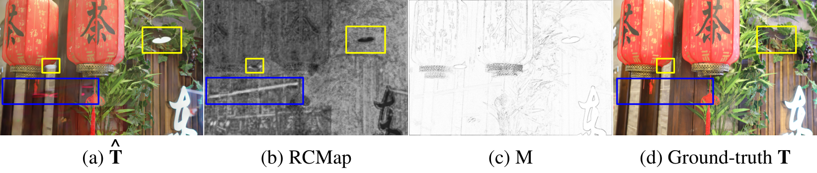
However, when the strong reflection regions are not correctly detected, our method still lacks cues to remove such reflections. For instance, there are remained highlights in the 4th row of our results in Fig. 6. As shown in Fig. 7, compared to the detected rod-shaped reflection (blue boxes), the two oval highlights (yellow boxes) are not completely detected. Hence, they still appear in the removal result. Although hard boundaries for these highlights exist in the inverse Laplacian map, our network still lacks enough context information to classify such oval highlights as reflections.
5.2 Ablation Study
To better analyze our network’s architecture and evaluate the importance of the loss functions, we perform ablation studies by manipulating the model components, removing or replacing loss functions. The statistics of PSNR and SSIM are obtained by evaluating the re-trained models in these experiments.
Evaluation of the network architecture. In Tab. 2, we first show that three modules in our network, namely RDM, TSM, and LSTM, all contribute to the SIRR performance (first three rows). We then test six different choices in the design of RDM, and the results are shown in the last six rows in Tab. 2. Our current design choices of RDM lead to the highest PSNR and SSIM scores. In addition, Fig. 8 illustrates the visual results of the ablation studies in Tab. 2.
| Model | SIR2 [41] | Zhang et al.[57] | Li et al.[23] | |||
| PSNR | SSIM | PSNR | SSIM | PSNR | SSIM | |
| w/o RDM & TSM | 23.237 | 0.881 | 22.784 | 0.800 | 22.607 | 0.778 |
| w/o TSM | 23.304 | 0.882 | 22.139 | 0.805 | 23.088 | 0.799 |
| w/o LSTM | 23.808 | 0.887 | 21.040 | 0.760 | 22.721 | 0.794 |
| from | 22.595 | 0.888 | 21.747 | 0.792 | 22.283 | 0.792 |
| MLSM SLSM | 23.089 | 0.879 | 21.708 | 0.796 | 23.065 | 0.800 |
| Fix MLSM | 23.640 | 0.891 | 22.951 | 0.809 | 22.646 | 0.802 |
| 23.612 | 0.892 | 22.381 | 0.808 | 23.234 | 0.798 | |
| LKI RKI | 24.106 | 0.893 | 21.784 | 0.791 | 22.224 | 0.794 |
| w/o GC in MLSM | 23.901 | 0.891 | 23.051 | 0.812 | 23.300 | 0.806 |
| Ours | 24.117 | 0.901 | 23.338 | 0.812 | 23.451 | 0.808 |

 |
 |
 |
 |
| (a) Input | (b) RCMap [RKI] | (c) RCMap [] | (d) RCMap [Ours] |
 |
 |
 |
 |
| (e) Ground-truth | (f) [RKI] | (g) [] | (h) [Ours] |
 |
 |
 |
 |
| (a) Input | (b) Ours [th.=0.5] | (c) | (d) |
Especially, to evaluate the effectiveness of Laplacian kernel initialization (LKI), we conduct an experiment by replacing LKI with random kernel initialization (RKI) using a Gaussian distribution (mean = 0, variance = 0.02) and cancel the gradient clipping. The PSNR/SSIM scores in the last second row of Tab. 2 show that LKI is superior to RKI. Moreover, a qualitative comparison is shown in the second and fourth columns in Fig. 9. The kernel learned by RKI tends to smooth out small-size reflections (yellow boxes) in its RCMap, leading to a downgraded reflection-removal result. In contrast, ours can successfully detect and remove the reflections. Moreover, the kernels learned by LKI and RKI are available in Sec.3 of the supplemental material.
Evaluation of loss functions. In Tab. 3, we report the performance of our model re-trained with ablated loss terms (first five rows). It can be seen that each loss term contributes to the network’s performance. We hypothesize that the performance drop after removing is due to the weight of SSIM loss is much larger than pixel loss in .
To verify the effectiveness of in detecting reflection-dominated regions, we compare it with the raindrop removal method in [30] that generates GT binary raindrop masks for the training. Specifically, we replace the with the combination of the binary cross-entropy (BCE) losses at different iterations:
| (16) |
where is set to 0.85. We follow the method in [30] to obtain the GT RCMaps: . First, we subtract the input image with its corresponding transmission image to obtain an absolute residual image , and then apply a threshold to to get a binary mask as , where is set to , and is the gray-scale . We re-train our model using and set the parameter to 0.3 for the best performance. The choice of is evaluated in Sec.4 of the supplemental material.
| Model | SIR2 [41] | Zhang et al. [57] | Li et al. [23] | |||
| PSNR | SSIM | PSNR | SSIM | PSNR | SSIM | |
| w/o | 23.365 | 0.888 | 22.113 | 0.788 | 21.587 | 0.788 |
| w/o | 15.653 | 0.673 | 17.652 | 0.746 | 15.197 | 0.642 |
| w/o | 22.725 | 0.880 | 22.219 | 0.804 | 22.778 | 0.812 |
| w/o | 23.774 | 0.894 | 22.453 | 0.807 | 23.036 | 0.801 |
| w/o | 23.571 | 0.889 | 22.480 | 0.803 | 23.240 | 0.800 |
| 24.106 | 0.894 | 21.296 | 0.776 | 22.176 | 0.788 | |
| & RKI | 24.114 | 0.899 | 21.123 | 0.778 | 22.253 | 0.788 |
| Ours | 24.117 | 0.901 | 23.338 | 0.812 | 23.451 | 0.808 |
As shown in Fig. 10, such a simple thresholding method occasionally generates GT RCMaps (the third column in Fig. 10) that incorrectly label some transmission-dominated regions with the reflection-dominated regions, even with relative intensity method (the last column in Fig. 10, ). We hypothesize that it is why our model based on surpasses the other two variants that use Eq. 16 and RKI in PSNR/SSIM scores, as shown in the last three rows of Tab. 3. Besides, the third column of Fig. 9 illustrates that the RCMap obtained under the supervision of ( = 0.3) contains mislabeling errors (red boxes), resulting in damages to non-reflection regions when estimating . In Sec.5 of the supplemental material, we evaluate the detection accuracy further and show that our method can well protect non-reflection regions.
6 Conclusion
We develop a location-aware SIRR network to improve the quality of SIRR results substantially. Its key feature is that we leverage learned Laplacian features that can emphasize the strong reflections’ boundaries to locate and remove strong reflections, such as reflected highlights. The network has an RDM that takes multi-scale Laplacian features as inputs to detect reflections roughly. In the future, we plan to simplify our network’s design further to save the number of parameters and improve its inference speed on the mobile computing platform.
Acknowledgements: We thank the reviewers for their constructive comments. Weiwei Xu is supported by NSFC (No. 61732016). This work was partially supported by a GRF grant from RGC of Hong Kong (Ref.: 11205620).
References
- [1] Nikolaos Arvanitopoulos, Radhakrishna Achanta, and Sabine Susstrunk. Single image reflection suppression. In CVPR, pages 4498–4506, 2017.
- [2] Yakun Chang and Cheolkon Jung. Single image reflection removal using convolutional neural networks. IEEE TIP, 28(4):1954–1966, 2018.
- [3] Bin Ding, Chengjiang Long, Ling Zhang, and Chunxia Xiao. Argan: Attentive recurrent generative adversarial network for shadow detection and removal. In ICCV, pages 10213–10222, 2019.
- [4] Qingnan Fan, Jiaolong Yang, Gang Hua, Baoquan Chen, and David Wipf. A generic deep architecture for single image reflection removal and image smoothing. In ICCV, pages 3238–3247, 2017.
- [5] Kun Gai, Zhenwei Shi, and Changshui Zhang. Blind separation of superimposed moving images using image statistics. IEEE TPAMI, 34(1):19–32, 2011.
- [6] Kshitiz Garg and Shree Nayar. Detection and removal of rain from videos. In CVPR, 2004.
- [7] Rafael Gonzalez, Richard Eugene Woods, and Steven Eddins. Digital Image Processing using MATLAB. Pearson, 2004.
- [8] Xiaojie Guo, Xiaochun Cao, and Yi Ma. Robust separation of reflection from multiple images. In CVPR, pages 2187–2194, 2014.
- [9] Kaiming He, Xiangyu Zhang, Shaoqing Ren, and Jian Sun. Delving deep into rectifiers: Surpassing human-level performance on imagenet classification. In ICCV, pages 1026–1034, 2015.
- [10] Sepp Hochreiter and Jürgen Schmidhuber. Long short-term memory. Neural computation, 9(8):1735–1780, 1997.
- [11] Jie Hu, Li Shen, and Gang Sun. Squeeze-and-excitation networks. In CVPR, pages 7132–7141, 2018.
- [12] Xiaowei Hu, Chi-Wing Fu, Lei Zhu, Jing Qin, and Pheng-Ann Heng. Direction-aware spatial context features for shadow detection and removal. IEEE TPAMI, 2019. to appear.
- [13] Xiaowei Hu, Yitong Jiang, Chi-Wing Fu, and Pheng-Ann Heng. Mask-shadowgan: Learning to remove shadows from unpaired data. In ICCV, pages 2472–2481, 2019.
- [14] Yan Huang, Yuhui Quan, Yong Xu, Ruotao Xu, and Hui Ji. Removing reflection from a single image with ghosting effect. IEEE Trans. on Computational Imaging, 6:34–45, 2019.
- [15] Meiguang Jin, Sabine Süsstrunk, and Paolo Favaro. Learning to see through reflections. In ICCP, pages 1–12, 2018.
- [16] Salman H Khan, Mohammed Bennamoun, Ferdous Sohel, and Roberto Togneri. Automatic shadow detection and removal from a single image. IEEE TPAMI, 38(3):431–446, 2015.
- [17] Jin-Hwan Kim, Chul Lee, Jae-Young Sim, and Chang-Su Kim. Single-image deraining using an adaptive nonlocal means filter. In ICIP, pages 914–917, 2013.
- [18] Soomin Kim, Yuchi Huo, and Sung-Eui Yoon. Single image reflection removal with physically-based training images. In CVPR, pages 5164–5173, 2020.
- [19] Diederik Kingma and Jimmy Ba. Adam: A method for stochastic optimization. arXiv:1412.6980, 2014.
- [20] Chenyang Lei, Xuhua Huang, Mengdi Zhang, Qiong Yan, Wenxiu Sun, and Qifeng Chen. Polarized reflection removal with perfect alignment in the wild. In CVPR, pages 1750–1758, 2020.
- [21] A. Levin and Y. Weiss. User assisted separation of reflections from a single image using a sparsity prior. IEEE TPAMI, 29(9):1647–1654, 2007.
- [22] Anat Levin, Assaf Zomet, and Yair Weiss. Learning to perceive transparency from the statistics of natural scenes. In NeurIPS, pages 1271–1278, 2003.
- [23] Chao Li, Yixiao Yang, Kun He, Stephen Lin, and John E Hopcroft. Single image reflection removal through cascaded refinement. In CVPR, pages 3565–3574, 2020.
- [24] Yu Li and Michael Brown. Single image layer separation using relative smoothness. In CVPR, pages 2752–2759, 2014.
- [25] Yu Li and Michael S Brown. Exploiting reflection change for automatic reflection removal. In ICCV, pages 2432–2439, 2013.
- [26] Ajay Nandoriya, Mohamed Elgharib, Changil Kim, Mohamed Hefeeda, and Wojciech Matusik. Video reflection removal through spatio-temporal optimization. In ICCV, pages 2411–2419, 2017.
- [27] Simon Niklaus, Xuaner Cecilia Zhang, Jonathan T Barron, Neal Wadhwa, Rahul Garg, Feng Liu, and Tianfan Xue. Learned dual-view reflection removal. In WACV, pages 3713–3722, 2021.
- [28] Adam Paszke, Sam Gross, Soumith Chintala, Gregory Chanan, Edward Yang, Zachary DeVito, Zeming Lin, Alban Desmaison, Luca Antiga, and Adam Lerer. Automatic differentiation in Pytorch. 2017.
- [29] Abhijith Punnappurath and Michael Brown. Reflection removal using a dual-pixel sensor. In CVPR, pages 1556–1565, 2019.
- [30] Rui Qian, Robby T Tan, Wenhan Yang, Jiajun Su, and Jiaying Liu. Attentive generative adversarial network for raindrop removal from a single image. In CVPR, pages 2482–2491, 2018.
- [31] Liangqiong Qu, Jiandong Tian, Shengfeng He, Yandong Tang, and Rynson WH Lau. Deshadownet: A multi-context embedding deep network for shadow removal. In CVPR, pages 4067–4075, 2017.
- [32] Olga Russakovsky, Jia Deng, Hao Su, Jonathan Krause, Sanjeev Satheesh, Sean Ma, Zhiheng Huang, Andrej Karpathy, Aditya Khosla, Michael Bernstein, et al. Imagenet large scale visual recognition challenge. IJCV, 115(3):211–252, 2015.
- [33] Bernard Sarel and Michal Irani. Separating transparent layers through layer information exchange. In ECCV, pages 328–341. Springer, 2004.
- [34] YiChang Shih, Dilip Krishnan, Fredo Durand, and William T Freeman. Reflection removal using ghosting cues. In CVPR, pages 3193–3201, 2015.
- [35] Christian Simon and In Kyu Park. Reflection removal for in-vehicle black box videos. In CVPR, pages 4231–4239, 2015.
- [36] Karen Simonyan and Andrew Zisserman. Very deep convolutional networks for large-scale image recognition. arXiv:1409.1556, 2014.
- [37] Sudipta N Sinha, Johannes Kopf, Michael Goesele, Daniel Scharstein, and Richard Szeliski. Image-based rendering for scenes with reflections. ACM TOG, 31(4):1–10, 2012.
- [38] Chao Sun, Shuaicheng Liu, Taotao Yang, Bing Zeng, Zhengning Wang, and Guanghui Liu. Automatic reflection removal using gradient intensity and motion cues. In ACM Multimedia, pages 466–470, 2016.
- [39] Richard Szeliski, Shai Avidan, and Padmanabhan Anandan. Layer extraction from multiple images containing reflections and transparency. In CVPR, pages 246–253, 2000.
- [40] Renjie Wan, Boxin Shi, Ling-Yu Duan, Ah-Hwee Tan, Wen Gao, and Alex C Kot. Region-aware reflection removal with unified content and gradient priors. IEEE TIP, 27(6):2927–2941, 2018.
- [41] Renjie Wan, Boxin Shi, Ling Yu Duan, Ah Hwee Tan, and Alex Kot. Benchmarking single-image reflection removal algorithms. In ICCV, 2017.
- [42] Renjie Wan, Boxin Shi, Tan Ah Hwee, and Alex C Kot. Depth of field guided reflection removal. In ICIP, pages 21–25, 2016.
- [43] Renjie Wan, Boxin Shi, Haoliang Li, Ling-Yu Duan, and Alex Kot. Face image reflection removal. IJCV, pages 1–15, 2020.
- [44] Renjie Wan, Boxin Shi, Haoliang Li, Ling-Yu Duan, Ah-Hwee Tan, and Alex Kot Chichung. Corrn: Cooperative reflection removal network. IEEE TPAMI, 42(12):2969–2982, 2020.
- [45] Jifeng Wang, Xiang Li, and Jian Yang. Stacked conditional generative adversarial networks for jointly learning shadow detection and shadow removal. In CVPR, pages 1788–1797, 2018.
- [46] Kaixuan Wei, Jiaolong Yang, Ying Fu, David Wipf, and Hua Huang. Single image reflection removal exploiting misaligned training data and network enhancements. In CVPR, pages 8178–8187, 2019.
- [47] Qiang Wen, Yinjie Tan, Jing Qin, Wenxi Liu, Guoqiang Han, and Shengfeng He. Single image reflection removal beyond linearity. In CVPR, pages 3771–3779, 2019.
- [48] Sanghyun Woo, Jongchan Park, Joon-Young Lee, and In So Kweon. Cbam: Convolutional block attention module. In ECCV, pages 3–19, 2018.
- [49] Tianfan Xue, Michael Rubinstein, Ce Liu, and William T Freeman. A computational approach for obstruction-free photography. ACM TOG, 34(4):1–11, 2015.
- [50] Jie Yang, Dong Gong, Lingqiao Liu, and Qinfeng Shi. Seeing deeply and bidirectionally: A deep learning approach for single image reflection removal. In ECCV, pages 654–669, 2018.
- [51] Wenhan Yang, Robby T Tan, Jiashi Feng, Zongming Guo, Shuicheng Yan, and Jiaying Liu. Joint rain detection and removal from a single image with contextualized deep networks. IEEE TPAMI, 42(6):1377–1393, 2019.
- [52] Yang Yang, Wenye Ma, Yin Zheng, Jian-Feng Cai, and Weiyu Xu. Fast single image reflection suppression via convex optimization. In CVPR, pages 8141–8149, 2019.
- [53] Leonid Yaroslavsky. Digital picture processing: an introduction, volume 9. Springer Science & Business Media, 2012.
- [54] Rajeev Yasarla and Vishal M Patel. Uncertainty guided multi-scale residual learning-using a cycle spinning cnn for single image de-raining. In CVPR, pages 8405–8414, 2019.
- [55] Shaodi You, Robby T Tan, Rei Kawakami, Yasuhiro Mukaigawa, and Katsushi Ikeuchi. Adherent raindrop modeling, detection and removal in video. IEEE TPAMI, 38(9):1721–1733, 2015.
- [56] Huaidong Zhang, Xuemiao Xu, Hai He, Shengfeng He, Guoqiang Han, Jing Qin, and Dapeng Wu. Fast user-guided single image reflection removal via edge-aware cascaded networks. IEEE TMM, 22(8):2012–2023, 2019.
- [57] Xuaner Zhang, Ren Ng, and Qifeng Chen. Single image reflection separation with perceptual losses. In CVPR, pages 4786–4794, 2018.
- [58] Hang Zhao, Orazio Gallo, Iuri Frosio, and Jan Kautz. Loss functions for neural networks for image processing. arXiv:1511.08861, 2015.