Probing quantum effects with classical stochastic analogs
Abstract
We propose a method to construct a classical analog of an open quantum system, namely a single quantum particle confined in a potential well and immersed in a thermal bath. The classical analog is made out of a collection of identical wells where classical particles of mass are trapped. The distribution of the classical positions is used to reconstruct the quantum Bohm potential , which in turn acts on the shape of the potential wells. As a result, the classical particles experience an effective “quantum” force. This protocol is tested with numerical simulations using single- and double-well potentials, evidencing typical quantum effects such as long-lasting correlations and quantum tunneling. For harmonic confinement, the analogy is implemented experimentally using micron-sized dielectric beads optically trapped by a laser beam.
I Introduction
Analogies in physics constitute a powerful tool for the understanding of complex phenomena. Not only they enable us to apply our knowledge and intuition of a specific domain to a different field, but also offer the possibility to transfer experimental results from one branch of physics to another. For instance, table-top experiments have been used to get insight into complex – and experimentally unreachable – domains such as quantum gravity and black holes, using acoustic Barceló et al. 2011 or optic Roger et al. 2016 analogs. Of particular interest here are classical analogs of quantum systems Dragoman and Dragoman 2004, based on optic Bouwmeester et al. 1995 or hydrodynamic Couder et al. 2005; Pucci et al. 2018 experiments. These analogs rely on the Madelung representation of the wave function and the corresponding “hydrodynamic” evolution equations for its amplitude and phase, as in the de Broglie-Bohm version of quantum mechanics Madelung 1927; Bohm 1952; Takabayasi 1954.
When a quantum particle is immersed in a thermal bath, and taking the limit of vanishing mass, the hydrodynamic model can be cast in the form of a quantum drift-diffusion (QDD) equation Degond et al. 2005; Pinneau 2002, which is often used to describe charge transport in semiconductor devices. Here, the QDD equation will be the starting point of our quantum-classical analogy. Indeed, the QDD model has the form of a classical Fokker-Planck equation with the addition of an extra Bohm potential , which depends on the position probability distribution of the particles and carries the information about quantum correlations. As is well know, any Fokker-Planck equation is equivalent to a stochastic process described by a Langevin equation.
Our goal here is to use such underlying classical stochastic process to emulate the evolution of a quantum system. For the present case, the situation is somewhat more complicated, because the Bohm potential depends on the position probability distribution, making the process nonlinear, as the random variable depends on its own probability density. These types of stochastic processes are known as McKean-Vlasov processes McKean 1966 and have been extensively studied in the past Kolokoltsov 2010.
Here, we devise a classical analog of this process by reconstructing the probability distribution by statistical means. Our strategy is based on the possibility of simultaneously manipulating many classical objects, whose ensemble distribution is used as an input to construct the Bohm potential, thus recovering the results of the QDD model. This can be achieved numerically by simulating stochastic trajectories, but, most importantly, can also be realized experimentally, by means of multiple optical trapping of micron-sized Brownian particles Rosales-Cabara et al. 2020, as illustrated schematically in Fig. 1. Experimentally, up to a few thousand traps can be realized in practice Bakr et al. 2009; Wang et al. 2020.
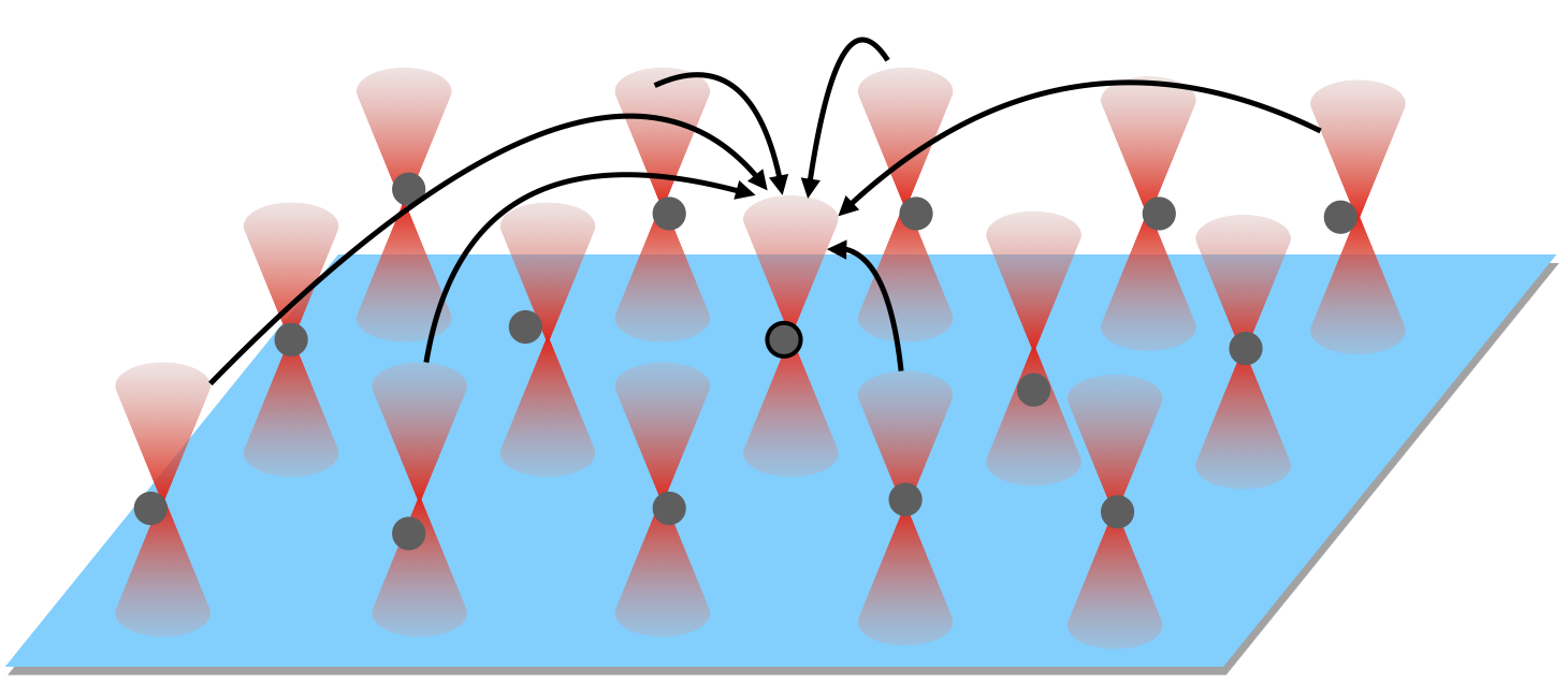
In this work, we will focus on three configurations that nicely capture some typical quantum effects: (i) a quantum increase of the position autocorrelation time, (ii) an analog of the quantum tunneling effect, and (iii) a departure from the classical dynamics for out-of-equilibrium states. These effects will be investigated with both numerical simulations, (i) and (ii), and optical experiments (iii).
II Model
The dynamics of a quantum particle interacting with a classical thermal environment can be described, in a first approximation, by a Wigner-Boltzmann equation Manfredi et al. 2019 (for a single spatial dimension, which is relevant here):
| (1) | ||||
where , is the Wigner phase-space distribution, is the external potential, and is a collision operator that models the interaction with the thermal bath. For instance, one could choose a relaxation operator , where is an equilibrium Maxwellian with bath temperature and is the thermalization time. Using a moment expansion of the Wigner-Boltzmann equation Gardner 1994; Manfredi 2005; Manfredi et al. 2019 and assuming an ideal-gas equation of state for the pressure , one can arrive at a set of two quantum hydrodynamic equations for the density and the mean velocity :
| (2) | |||||
| (3) |
where is Boltzmann’s constant, is the mass of the quantum object, and is Planck’s constant. Quantum effects are contained in the Bohm potential: .
It is natural to choose , where is the drag coefficient of the object in the fluid that makes up the thermal bath. Finally, taking the limit and , while remains finite, enables us to drop the inertial terms [left-hand side of Eq. (3)] and to inject the expression for into the continuity equation (2), leading to a single quantum drift-diffusion (QDD) equation for the density Pinneau 2002:
| (4) |
This equation has the structure of a classical Fokker-Planck equation for Brownian motion, and differs from it only by the presence of the Bohm potential. This is an important difference, however, as the Bohm potential is itself a functional of the probability density and its derivatives. The stochastic process underlying Eq. (4) belongs to the class of McKean-Vlasov processes McKean 1966; Kolokoltsov 2010, describing random variables whose trajectories depend on their own probability distribution. The Langevin equation of the stochastic process associated with Eq. (4) can be written as:
| (5) |
where is the Wiener increment due to white noise, with zero mean and no memory .
The stochastic/diffusive model of Eqs. (4) and (5) describes a quantum system coupled to a classical thermal bath. The coupling will induce some level of decoherence, leading to the partial loss of the quantum character of our system. Nevertheless, some quantum properties will persist in spite of the decoherence, notably those encapsulated in the Bohm potential. The aim of this work is to emulate such quantum properties using a purely classical experimental setup.
In order to emulate Eq. (5) the key issue is to be able to inject the probability distribution into the stochastic process itself. This can be achieved with a classical system if one can generate (numerically or experimentally) simultaneous trajectories in order to reconstruct , and hence the Bohm potential, at each time-step. Experimentally, this may be implemented using a multiple optical trapping system (see Fig. 1).
Equation (5) can be rewritten in a normalized form that brings out a dimensionless parameter , which plays the role of a normalized Planck constant and governs the strength of the quantum effects. The quantity can be interpreted as the ratio between the quantum decoherence time and the classical relaxation time (see Appendix A). In our classical analog, is no longer related to Planck’s constant, but can be adjusted at will, within the practical limits of the experimental or numerical realization. The classical case, i.e. standard Brownian motion, corresponds to , while when “quantum” effects play a significant role.
III Numerical results
We use a quartic external potential . We consider two cases, with either (anharmonic single well) or (bistable double-well potential), and focus on the features of the equilibrium distribution. Transients will be analyzed later using an experimental protocol. Simulations are performed with a first-order Euler-Maruyama algorithm Volpe and Volpe 2013; Kloeden and Platen 1992 that solves the McKean-Vlasov equation (5) for trajectories simultaneously. At each time-step, a smooth distribution is constructed from the trajectories by softening the particle positions with a Gaussian kernel. Details are given in the Appendix B. We take as the initial condition the stationary distribution of a classical process (), then turn on quantum effects () and let the system evolve to its new equilibrium.


In the case, the confining potential is a single quartic well. In Fig. 2 (top left) we represent some simulated trajectories. After a certain relaxation time, the system stabilizes around a quantum equilibrium distribution, which differs significantly from the initial classical Boltzmann equilibrium (top right). This departure from the classical result is due to the Bohm force, which works against the external confinement, as detailed in the Appendix C.
In Fig. 2 (bottom frame), we show the normalized autocorrelation at equilibrium: , where the average is over all the trajectories, as a function of the lag-time . The initial time is set at an instant , when the distribution has already relaxed to its quantum equilibrium. We note that the addition of the quantum Bohm potential induces longer-lasting correlations compared to the classical case. A straightforward interpretation is that the McKean-Vlasov trajectories are correlated with one another through the action of the Bohm force.
We now turn to the case , for which the confining potential is a bistable double well. Using the same numerical method, we simulate trajectories for both the classical () and the McKean-Vlasov () stochastic processes. In the classical case, the trajectories linger in one of the wells for a relatively long residency time , before occasionally jumping to the second well due to thermal fluctuations. In contrast, in the McKean-Vlasov case these jumps occur much more frequently (Fig. 3, top left frame). The jump events are correctly described by Poisson statistics Grebenkov 2014; Mandel 1979 and the probability distribution of the residency times obeys an exponential decay law Simon and Libchaber 1992 , where . The results shown in Fig. 3 (bottom frame) are in good agreement with this Poissonian law, both for the classical and for the McKean-Vlasov processes, albeit with different values of , the effect of the Bohm potential being to decrease the mean residency time. The enhanced mobility between the two wells is clearly seen in the probability distribution of the particle positions (top right frame), which signals a decrease of the effective potential barrier due to the quantum Bohm potential. This result can be interpreted as a manifestation of quantum tunneling, which increases the frequency of barrier-crossing events beyond the classical thermally-induced probability. We emphasize that this quantum-like property persists despite the decoherence that is inherent to our model.


IV Experimental realization
Next, we turn to the possibility of implementing experimentally our classical-quantum analog. For this, we adopt a harmonic confinement potential , which is easy to realize with an optical trap, and also allows us to circumvent the need of using many traps to implement the analog process. This approach will be used to study the effect of the Bohm potential in an out-of-equilibrium configuration.
First, we note Burghardt and Moller 2002 that a Gaussian probability distribution: , where is the time-dependent variance of the distribution, is an exact solution of the McKean-Vlasov process (5), provided the variance obeys the following equation:
| (6) |
Furthermore, for such Gaussian distribution the Bohm force takes a simple analytical form: . In this case, both the external force and the Bohm force have the same functional form, linear in the stochastic variable , and can therefore be grouped together into a single harmonic term with modified stiffness: . Hence, the quantum McKean-Vlasov process can be expressed as an ordinary (Ornstein-Uhlenbeck) stochastic process:
| (7) |
Despite this apparent mathematical simplicity, all the physical richness of the analog model is preserved, with the modified stiffness still depending on the ensemble variance as a consequence of the quantum nature of the problem. Moreover, in this harmonic case, the dimensionless parameter governing quantum effects takes the form: , i.e. half the ratio between the de Broglie thermal wavelength and the classical width of the harmonic oscillator at thermal equilibrium . The specificity of the harmonic confinement is that the variance need not be measured out of a collection of trajectories taking place simultaneously in identical traps, as in Fig. 1. Instead, can be computed from Eq. (6) and then used to construct the Bohm potential or force, thus avoiding the necessity of using many optical traps in the experiment.

Our experimental setup – presented in detail in the Appendix D – is composed of a single dielectric bead optically trapped by a Gaussian laser beam. The optical potential created by the gradient forces at the waist of the beam is harmonic, with a stiffness that is proportional to the intensity of the laser and can thus be controlled precisely. The bead is immersed in water at ambient temperature and undergoes Brownian motion due to the thermal fluctuations. The overall motion is consistent with an Ornstein-Uhlenbeck process and is therefore suited to implement our model.
Here, we use the above approach to study out-of-equilibrium evolutions with a time-dependent stiffness . The simplest possible out-of-equilibrium process is the transient occurring when the stiffness is suddenly changed from an initial value to a final value (step-like protocol). The system is at thermal equilibrium at the initial and final times. The transient evolution of the variance can be computed using Eq. (6), allowing us to construct the modified stiffness , which evolves from to in a non-trivial way due to the influence of . One can argue that, since different values of lead to different values of for the initial and final equilibria, the classical () and quantum (here, ) transients are difficult to compare, as they do not begin and end with the same values of the stiffness. With this in mind, we also implemented an equivalent classical protocol that goes from to in a step-like way, i.e. without the dynamical influence of the Bohm force. These two protocols, represented in the inset of Fig. 4, connect the same initial and final equilibria, and are thus well-suited to compare the classical and quantum dynamics out-of-equilibrium.
Finally, in order to obtain ensemble averages out of our single trajectory, we rely on the ergodic hypothesis and use a time-series of trajectories instead of a statistical ensemble. We send the same protocol at a low enough repetition rate so that equilibrium is reached between two consecutive events, and then reconstruct a synchronized ensemble from this time series. The result is an ensemble of over trajectories experiencing a given protocol, either in the quantum case or in the classical case.
The main observable of interest here is the time evolution of the ensemble variance, represented in Fig. 4 for both the quantum and classical cases. Our measurements clearly reveal the influence of the Bohm force on . Strikingly, the addition of an effective quantum force accelerates its relaxation, and this for all selected values of , as detailed in the Appendix D. Looking at in the McKean-Vlasov process (Fig. 4, inset), the acceleration appears as the result of a strong and sudden reduction of the optical trapping volume under the influence of the quantum Bohm force field. On each curve, we also represent the result of numerical simulations, where the evaluation of the Bohm term is not performed through the solution of Eq. (6), but by actually computing the ensemble variance of distinct trajectories at each time-step. The agreement of both the experimental and numerical results with the analytical solution of Eq. (6) is quite remarkable.
V Conclusion
We highlighted an analogy between an open quantum system immersed in a thermal bath and a classical nonlinear stochastic process (McKean-Vlasov process). This correspondence opened up the possibility to build a classical analog of the quantum model, by evolving many stochastic trajectories in parallel and using their distribution to reconstruct the quantum Bohm potential. This classical analog was realized both numerically and experimentally, evidencing typical quantum effects such as long-lasting correlations and quantum tunneling.
The present work is a first step in the experimental implementation of classical analogs of quantum systems using optically trapped Brownian particles, which should provide an original platform for probing the subtle connections between quantum mechanics and stochastic thermodynamics. We emphasize that our approach is obviously not limited to the QDD framework, whose validity is constrained by several conditions. It can, for instance, be extended to classically emulate fully quantum evolutions, described in the most general scenario by the time-dependent Schrödinger equation. This non-trivial generalization should lead to classical stochastic systems specifically designed to access the controlled exploration of many fundamental quantum effects, such as quantum correlations, quantum decoherence, and quantum chaos.
Acknowledgements
This work of the Interdisciplinary Thematic Institute QMat, as part of the ITI 2021 2028 program of the University of Strasbourg, CNRS and Inserm, was supported by IdEx Unistra (ANR 10 IDEX 0002), by SFRI STRAT’US project (ANR 20 SFRI 0012), by the Labex NIE (ANR-11-LABX-0058 NIE) and CSC (ANR-10-LABX-0026 CSC) projects, and by the University of Strasbourg Institute for Advanced Study (USIAS) (ANR-10-IDEX-0002-02) under the framework of the French Investments for the Future Program.
Appendix A Nondimensionalization of the McKean-Vlasov process
In order to derive a non-dimensional description of the QDD equation for , we start with
| (8) |
and make the following change of variables, focusing on a quadratic external potential for simplicity:
| (9) |
Here, corresponds to the initial stiffness, is the corresponding relaxation time and the classical width of the harmonic oscillator at thermal equilibrium fixed by equipartition. This change of variables leads to
| (10) |
where is the dimensionless parameter described in the main text. The non-dimensional stochastic McKean-Vlasov process then writes as:
| (11) |
As discussed in the main text, can be written as half the ratio between the de Broglie thermal length and the classical width of the harmonic oscillator at thermal equilibrium . Another possible interpretation can be given as the ratio between the quantum decoherence time and the thermal relaxation time . Following Zurek 2007, the loss of quantum coherence is governed by a typical time scale where is a typical length scale of motion. In our case, we take . This gives , i.e., the ratio between the decoherence time and the relaxation time.
Appendix B Numerical method
Our numerical approach is based on the Euler-Maruyama stochastic algorithm Volpe and Volpe 2013; Kloeden and Platen 1992. It consists in a discrete approximation of the stochastic differential equation up to order in the time increment . For the stochastic equation
where all variables are non-dimensional, it takes the form
| (12) |
where is the numerical approximation of , is a normally distributed random variable, and is the time-step.
Our numerical approach is the following: like for a classical stochastic algorithm, we compute the positions at a certain time-step for Brownian particles simultaneously and then evaluate the forces for the next time-step. The specificity of the present case arises from the evaluation of the quantum force, which requires the reconstruction of the density . We use a particle-in-cell method to evaluate : to each particle we associate a Gaussian kernel of width , and the sum of such Gaussians will yield a reasonably smooth estimation of the density . From this reconstructed density we are able to compute the quantum force , which in turn is used to update the positions of the particles at the next time-step.
One important parameter here is the width of the Gaussian kernel. Too small a width will lead to a noisy evaluation of the density, which is dangerous because the quantum force requires the computation of the third derivative of the density. The problem mainly arises when we use few trajectories, as we do in our work in order to stay close to the experiments. In our case, where trajectories are employed, we made a reasonable compromise between a kernel of width , i.e., a sum of Dirac delta functions, and a width (in normalized units) which would amount to a Gaussian approximation for the whole density. We use a value which is large enough to smooth out irregularities arising from the small statistical sample, but small enough to account for departures from a perfectly Gaussian density (as evidenced from the skewness and kurtosis, see Appendix C). The histograms of the particles distributions and the corresponding smooth densities are shown in Fig. 5.

Appendix C Statistical analysis


In Fig. 6, we represent a logarithmic plot of the final distribution of simultaneous trajectories for three different cases: (i) classical process in a confining quartic potential, (ii) McKean-Vlasov process in a quartic potential, and (iii) classical Ornstein-Uhlenbeck process in a quadratic potential. We also show the fitting of the distribution with two models: the Ornstein-Uhlenbeck final distribution is fitted with a Gaussian distribution, while the other two cases are fitted with a model of the form , which is a classical Maxwell-Boltzmann distribution in a quartic potential. We see that the McKean-Vlasov final distribution also belongs to this category, which means that the Bohm potential in this case takes the form of a quartic-type potential. We also represent the first moments of the distributions in order to obtain more detailed information. We note that the quantum and classical cases in a quartic potential (orange and blue lines) differ mostly by their respective variances, whereas their kurtosis (describing their tailedness) are similar, departing noticeably from the Gaussian value. The skewnesses, as expected, are zero since all distributions are symmetrical.

In Fig. 7 we represent the Bohm force in the quartic case, along with a third order polynomial fit and the Gaussian limit. We see that the agreement of the fit is good, showing that in this case again, the Bohm potential takes a form similar to the external potential.
Appendix D Experimental setup and calibration

Our experiment, schematized in Fig. 8, consists in trapping a single Brownian object in the harmonic potential created by a focused laser beam. A linearly polarized Gaussian beam (CW 785 nm diode) is focused by a water immersion objective (Nikon Plan-Apo VC, Numerical Aperture Water Immersion) into a fluidic cell of m thickness filled with deionized water with a monodispersed suspension of polystyrene microspheres (Thermoscientific Fluoro-Max, radius nm). We make sure that only one single bead is trapped at the waist of the focused beam, using an interferometric scattering microscopy system (not shown on the figure) Lindfors et al. 2004.
The position of the bead is recorded using a low-power counter-propagating laser beam (639 nm diode), focused on the bead using a second objective (Nikon Plan-fluo ELWD 60x0.70). The light scattered by the bead is recollected and send to a photodiode (Thorlabs Det10A). The signal recorded (in V/s) is send to a low noise amplifier (SR560) and then acquired by an analog-to-digital card (NI PCI-6251). The signal is filtered through a Hz high-pass filter at 6 dB/oct to remove the DC component and through a kHz low-pas filter at 6 dB/oct to prevent from aliasing. The position of the bead along the optical axis is, for small enough displacements linear with the scattered intensity. Furthermore, we work in the linear regime of our photodiodes so that the signal remains linear with the intensity. Finally, the resulting voltage trace is also linear with the instantaneous position of the trapped bead.
In our experimental implementation, the optical potential created by the focused laser beam is locally harmonic. The stiffness of the harmonic potential is proportional to the laser power and can be controlled by the experimentalist. Our experimental method and calibration are based on the theoretical results obtained in the harmonic and Gaussian case, mainly the relation between the stiffness and the variance given by Eq. (6). It makes it possible to realize the McKean-Vlasov process using one single trajectory and to use this system to probe out-of-equilibrium states, with a given protocol . The method is the following: first a protocol is defined, a value of the parameter is chosen and is transferred to an arbitrary Planck constant . Then the variance ODE is solved for this protocol and the modified stiffness is injected as a laser intensity protocol. The different steps of the procedure including the calibration are summarized Fig. 9.
This procedure however relies on a precise calibration of the system: in order to use the variance differential equation, we need to know with the best possible precision the stiffness at play in the trap. In this section, we detail our method.

In order to predict the stiffness in the trap, we first calibrate the linear relation between the trapping laser power and . We use the power spectral density (PSD) method Berg-Sørensen and Flyvbjerg 2004. The Ornstein-Uhlenbeck process describes the Brownian motion in the trap
where is Stokes coefficient given by where is water viscosity and the beads radius. This process can be spectrally analysed with the position PSD:
| (13) |
where the roll-off frequency separates the high frequency regime of free Brownian motion from the low frequency trapping regime . By recording a trajectory with a certain laser power, one can obtain the stiffness from the roll-off , by a Lorentzian fit of the spectrum. In Fig. 10 (left) we represent the PSD and fit for different trapping strength that gives the linear relation between and the laser power. It is then possible to send a designed protocol of stiffness by inverting the relation.


In order to build an ensemble of synchronised trajectories experiencing a defined protocol, we rely on the ergodic hypothesis. From one long trajectory experiencing a series of protocols, we build an ensemble of trajectories. We start by defining a step-like protocol where goes abruptly from to and send it as to the trapping laser. From the obtained ensemble of trajectories experiencing a transient relaxation, we extract the photodiode signal variance that follows an exponential decay (solution of the classical Fokker-Planck equation). This decay is fully characterising the final stiffness. With an exponential fit of both the ”up” and ”down” stiffness steps, we recover a measurement of the stiffness performed in the time-domain. This allows us to measure, during the experiment the actual stiffness at play that can depart slightly from the expected value, due to small drifts or to fit errors of the Lorentzian Berg-Sørensen and Flyvbjerg 2004. Since we double each McKean-Vlasov experiment with an equivalent classical step, we can perform this dynamical calibration for each experiment.
After the first step-like protocol experiment, we define a value of and perform both the quantum and the classical analog experiments. The dynamical calibration gives the values of and , that yield an that can slightly differ from the predicted value. These values correspond to the parameters needed for the analytical results.
Furthermore, the variance and the stiffness are unambiguously connected by the variance differential equation . Hence, once we know the stiffness, we can compute and can then calibrate our measured voltage variance to . We fit the transformation by a linear relationship which implies that the position transforms according to where the first term represents the linear response of the photodiode and the second the sum of all experimental noises (that we approximate as a resulting white noise). This method allows a precise calibration of the variance, as seen on Fig. 11, which is our only observable here. This method gives the position itself only up to the noise therm, which is several order of magnitude smaller than the term.


The error on the experimental variance essentially comes from three main sources. One is the error on the experimental parameters such as the temperature or the radius of the trapped bead, through the viscous drag coefficient . It is dominated by the uncertainties on the beads radius that result in a similar error on where is the water viscosity. Other sources of errors (temperature) are also taken into account but their final influence is not significant. Temperature in particular is controlled with a precision better than K. The error on the radius is simply taken into account by carrying the whole analysis with the two ”worst” values of radius, yielding an error between the two extreme results. The second source of errors is the statistical reliability of an estimator of the variance on an ensemble of finite size. It is obtained following the test on degrees of freedom, where is the size of the ensemble. We carry the test with confidence interval giving . The third source is the error arising from the fitting procedure in the calibration of the decay to obtain the stiffness and to calibrate the variance from to giving . The obtained variance is then defined up to:
| (14) |
These different error sources give the colored patch shown on each plot of Fig. 11.
References
- Barceló et al. (2011) Carlos Barceló, Stefano Liberati, and Matt Visser, “Analogue gravity,” Living Reviews in Relativity 14, 3 (2011).
- Roger et al. (2016) Thomas Roger, Calum Maitland, Kali Wilson, Niclas Westerberg, David Vocke, Ewan M. Wright, and Daniele Faccio, “Optical analogues of the Newton-Schrödinger equation and boson star evolution,” Nature Commun. 7, 13492 (2016).
- Dragoman and Dragoman (2004) D. Dragoman and M. Dragoman, Quantum-Classical Analogies (Springer, 2004).
- Bouwmeester et al. (1995) D. Bouwmeester, N. H. Dekker, F. Dorsselaer, C.A. Schrama, P. M. Visser, and J. P. Woerdman, “Observation of Landau-Zener dynamics in classical optical systems,” Physical Review A 51, 646–654 (1995).
- Couder et al. (2005) Y. Couder, S. Protière, E. Fort, and A. Boudaoud, “Walking and orbiting droplets,” Nature 437, 208–208 (2005).
- Pucci et al. (2018) Giuseppe Pucci, Daniel M. Harris, Luiz M. Faria, and John W. M. Bush, “Walking droplets interacting with single and double slits,” Journal of Fluid Mechanics 835, 1136–1156 (2018).
- Madelung (1927) E Madelung, “Quantum theory in hydrodynamical form,” Zeit. f. Phys. 40, 322 (1927).
- Bohm (1952) David Bohm, “A suggested interpretation of the quantum theory in terms of hidden variables,” Physical Review 85, 166–179 (1952).
- Takabayasi (1954) Takehiko Takabayasi, “The formulation of quantum mechanics in terms of ensemble in phase space,” Progress of Theoretical Physics 11, 341–373 (1954).
- Degond et al. (2005) Pierre Degond, Florian Méhats, and Christian Ringhofer, “Quantum energy-transport and drift-diffusion models,” Journal of Statistical Physics 118, 625–667 (2005).
- Pinneau (2002) R. Pinneau, “A review on the quantum drift diffusion model,” Transport Theory and Statistical Physics 31, 367–395 (2002).
- McKean (1966) H. P. McKean, “A class of Markov processes associated with nonlinear parabolic equations,” Proc. Natl. Acad. Sci. 56, 1907–1911 (1966).
- Kolokoltsov (2010) Vassili N. Kolokoltsov, Nonlinear Markov Processes and Kinetic Equations, Cambridge Tracts in Mathematics (Cambridge University Press, 2010).
- Rosales-Cabara et al. (2020) Yoseline Rosales-Cabara, Giovanni Manfredi, Gabriel Schnoering, Paul-Antoine Hervieux, Laurent Mertz, and Cyriaque Genet, “Optimal protocols and universal time-energy bound in brownian thermodynamics,” Phys. Rev. Research 2, 012012(R) (2020).
- Bakr et al. (2009) Waseem S. Bakr, Jonathon I. Gillen, Amy Peng, Simon Fölling, and Markus Greiner, “A quantum gas microscope for detecting single atoms in a Hubbard-regime optical lattice,” Nature 462, 74–77 (2009).
- Wang et al. (2020) Yibo Wang, Sayali Shevate, Tobias Martin Wintermantel, Manuel Morgado, Graham Lochead, and Shannon Whitlock, “Preparation of hundreds of microscopic atomic ensembles in optical tweezer arrays,” npj Quantum Information 6, 1–5 (2020).
- Manfredi et al. (2019) G. Manfredi, P.-A. Hervieux, and J. Hurst, “Phase-space modeling of solid-state plasmas,” Rev. Mod. Plasma Phys. 3, 13 (2019).
- Gardner (1994) Carl L. Gardner, “The quantum hydrodynamic model for semiconductor devices,” SIAM J. Appl. Math. 54, 409–427 (1994).
- Manfredi (2005) Giovanni Manfredi, “How to model quantum plasmas,” Fields Institute Communications Series 46, 263–287 (2005).
- Volpe and Volpe (2013) Giorgio Volpe and Giovanni Volpe, “Simulation of a Brownian particle in an optical trap,” Am. J. Phys. 81, 224–230 (2013).
- Kloeden and Platen (1992) Peter E. Kloeden and Eckhard Platen, Numerical Solutions of stochastic differential equations, Vol. 23 (Springer, 1992).
- Grebenkov (2014) Denis S Grebenkov, “First exit times of harmonically trapped particles: a didactic review,” Journal of Physics A: Mathematical and Theoretical 48, 013001 (2014).
- Mandel (1979) L. Mandel, “Sub-poissonian photon statistics in resonance fluorescence,” Opt. Lett. 4, 205–207 (1979).
- Simon and Libchaber (1992) Adam Simon and Albert Libchaber, “Escape and synchronization of a Brownian particle,” Phys. Rev. Lett. 68, 3375–3378 (1992).
- Burghardt and Moller (2002) I. Burghardt and K.B. Moller, “Quantum dynamics for dissipative systems: A hydrodynamical perspective,” Journal of Chemical Physics 117 (2002).
- Zurek (2007) Wojciech Hubert Zurek, “Decoherence and the transition from quantum to classical — revisited,” in Quantum Decoherence: Poincaré Seminar 2005, edited by Bertrand Duplantier, Jean-Michel Raimond, and Vincent Rivasseau (Birkhäuser Basel, Basel, 2007) pp. 1–31.
- Lindfors et al. (2004) K. Lindfors, T. Kalkbrenner, P. Stoller, and V. Sandoghdar, “Detection and spectroscopy of gold nanoparticles using supercontinuum white light confocal microscopy,” Phys. Rev. Lett. 93, 037401 (2004).
- Berg-Sørensen and Flyvbjerg (2004) Kirstine Berg-Sørensen and Henrik Flyvbjerg, “Power spectrum analysis for optical tweezers,” Review of Scientific Instruments 75, 594–612 (2004).