Transverse oscillation of a coronal loop induced by a flare-related jet
Abstract
Context. Kink oscillations in coronal loops are ubiquitous, and the observed parameters of oscillations are applied to estimate the magnetic field strength of the loops.
Aims. In this work, we report our multiwavelength observations of the transverse oscillation of a large-scale coronal loop with a length of 350 Mm. The oscillation was induced by a blowout coronal jet, which was related to a C4.2 circular-ribbon flare (CRF) in AR 12434 on 2015 October 16. We aim to determine the physical parameters in the coronal loop, including the Alfvén speed and magnetic field strength.
Methods. The jet-induced kink oscillation was observed in extreme-ultraviolet (EUV) wavelengths by the Atmospheric Imaging Assembly (AIA) on board the Solar Dynamics Observatory (SDO). Line of sight magnetograms were observed by the Helioseismic and Magnetic Imager (HMI) on board SDO. We took several slices along the loop to assemble time-distance diagrams, and used an exponentially decaying sine function to fit the decaying oscillation. The initial amplitude, period, and damping time of kink oscillation were obtained. Coronal seismology of the kink mode was applied to estimate the Alfvén speed and magnetic field strength in the oscillating loop. In addition, we measured the magnetic field of the loop through non-linear force-free field (NLFFF) modeling using the flux rope insertion method.
Results. The oscillation is most pronounced in AIA 171 and 131 Å. The oscillation is almost in phase along the loop with a peak initial amplitude of 13.6 Mm, meaning that the oscillation belong to the fast standing kink mode. The oscillation lasts for 3.5 cycles with an average period of 462 s and average damping time of 976 s. The values of lie in the range of 1.52.5. Based on coronal seismology, the Alfvén speed in the oscillating loop is estimated to be 1210 km s-1. Two independent methods are applied to calculate the magnetic field strength of the loop, resulting in 3043 G using the coronal seismology and 2123 G using the NLFFF modeling, respectively.
Conclusions. The magnetic field strength estimated using two different approaches are in the same order of magnitude, which confirms the reliability of coronal seismology by comparing with the NLFFF modeling.
Key Words.
Sun: magnetic fields – Sun: flare – Sun: corona – Sun: oscillations1 Introduction
Waves and oscillations are prevalent in the fully ionized solar corona with temperatures of several million Kelvin (MK) (see Nakariakov & Verwichte 2005, and refererence therein). The periodic transverse displacements of coronal loops are usually considered as kink oscillations detected in the extreme ultraviolet (EUV) wavelengths (Andries et al. 2009; Ruderman & Erdélyi 2009). Standing fast kink-mode oscillations were initially discovered by the Transition Region and Coronal Explorer (Handy et al. 1999, TRACE;) mission in 171 Å (Aschwanden et al. 1999; Nakariakov et al. 1999; Schrijver et al. 2002). Since the launch of the Solar Dynamics Observatory (Pesnell et al. 2012, SDO;), kink oscillations of coronal loops observed by the Atmospheric Imaging Assembly (Lemen et al. 2012, AIA;) on board SDO have been extensively investigated (Aschwanden & Schrijver 2011; White & Verwichte 2012; Verwichte et al. 2013a; Verwichte et al. 2013b; Pascoe et al. 2016; Nisticò et al. 2017; Duckenfield et al. 2018; Duckenfield et al. 2019; Nechaeva et al. 2019, e.g.,).
The commencement of the loop oscillation usually coincides with a nearby eruption (flare, jet, or filament eruption) in the lower corona, which is considered as the predominant mechanism for exciting kink oscillations (Zimovets & Nakariakov 2015). After the excitation, kink oscillations experience attenuation and last for several cycles in most cases (Goddard et al. 2016; Goddard & Nakariakov 2016). Resonant absorption, as a result of resonance within a finite thin layer, is believed to play a key role in the rapid damping of fast-mode kink oscillations (Goossens et al. 2002; Ruderman & Roberts 2002). Phase mixing with anomalously high viscosity is also important in the dissipation of energy during loop oscillations (Ofman & Aschwanden 2002). Small-amplitude, transverse oscillations of coronal loops without significant damping have been noticed (Anfinogentov et al. 2013; Nisticò et al. 2013; Li et al. 2018a; Zhang 2020). The observed loop oscillations in combination with magnetohydrodynamics (MHD) wave theory provide an effective tool to determine the local physical parameters, such as the magnetic field and Alfvén speed of the oscillating loops, which are difficult to measure directly (Edwin & Roberts 1983; Nakariakov & Ofman 2001; Aschwanden et al. 2002; Verwichte et al. 2006; Arregui et al. 2007; Goossens et al. 2008; Van Doorsselaere et al. 2008; Antolin & Verwichte 2011; Yuan & Van Doorsselaere 2016; Li et al. 2017).
Circular-ribbon flares (CRFs) are a special type of flares, whose short, inner ribbons are surrounded by circular or elliptical ribbons (Masson et al. 2009; Chen et al. 2019; Zhang et al. 2016b; Zhang et al. 2019; Lee et al. 2020; Liu et al. 2020). Transverse loop oscillations excited by CRFs with periods of 4 min have been observed by AIA (Zhang et al. 2015; Li et al. 2018b). Recently, Zhang et al. 2020 investigated the transverse oscillations of an EUV loop excited by two successive CRFs on 2014 March 5. The oscillations are divided into two stages in their development: the first-stage oscillation triggered by the C2.8 flare is decayless with lower amplitudes, and the second-stage oscillation triggered by the M1.0 flare is decaying with larger amplitudes. The authors also estimated the magnetic field and thickness of the inhomogeneous layer of the oscillating loop with a length of 130 Mm.
In this paper, we report our multiwavelength observations of the transverse oscillation of a large-scale coronal loop excited by a blowout jet associated with the C4.2 CRF in active region (AR) 12434 on 2015 October 16. Zhang et al. 2016c studied the explosive chromospheric evaporation at the inner and outer flare ribbons using spectroscopic observations. This work is building on the work of Zhang et al. 2016c (hereafter Paper I), and the main purpose is to estimate the magnetic field of the oscillating loop using two independent approaches, coronal seismology and magnetic field extrapolation. This paper is organized as follows. Observations and data analysis are presented in Sect. 2. The results are presented in Sect. 3. A brief summary and discussion are presented in Sect. 4.
2 Observations and Data Analysis
2.1 Instruments
The transverse oscillation of the coronal loop was observed by SDO/AIA, which has a spatial resolution of 12 and time cadence of 12 s in EUV wavelengths. The photospheric line-of-sight (LOS) magnetograms were observed by the Helioseismic and Magnetic Imager (Schou et al. 2012, HMI;) on board SDO with a spatial resolution of 12 and time cadence of 45 s. The level_1 data from AIA and HMI were calibrated using the standard Solar SoftWare (SSW) programs aia_prep.pro and hmi_prep.pro, respectively. Soft X-ray (SXR) light curves of the flare were recorded by the GOES spacecraft with a cadence of 2.05 s.
2.2 DEM analysis
The differential emission measure (DEM) analysis is a useful tool to perform temperature diagnostics. Several algorithms have been proposed and validated (Weber et al. 2004; Hannah & Kontar 2012; Aschwanden et al. 2013; Plowman et al. 2013; Cheung et al. 2015; Su et al. 2018b; Morgan & Pickering 2019, e.g.). The observed flux of each optically thin passband is determined by:
| (1) |
where is the temperature response function of passband , and DEM() represents the DEM of multithermal plasma as a function of temperature. and stand for the lower and upper limits for the integral. To carry out the inversion of DEM profile, we use the standard SSW program xrt_dem_iterative2.pro and six EUV passbands (94, 131, 171, 193, 211, and 335 Å). The method has been strictly justified and successfully applied to the temperature estimation of EUV hot channel as well as coronal jets (Cheng et al. 2012; Zhang & Ji 2014; Zhang et al. 2016a). Note that the background emissions should be removed before inversion.
The DEM-weighted average temperature is defined as (Cheng et al. 2012):
| (2) |
Then, the total column emission measure (EM) along the LOS is expressed as:
| (3) |
2.3 Flux rope insertion method
We use the flux rope insertion method developed by van Ballegooijen 2004 to reconstruct the non-linear force-free field (NLFFF) of AR 12434. The advantage of this method is that it can be applied to many different situations including both ARs (Su et al. 2009; Su et al. 2011; Su et al. 2018a) and quiet Sun (Su et al. 2015) since no vector field observations are required and the magnetic field lines of the best-fit model match well the observed coronal non-potential structures. Su 2019 gives a detailed review on the application of the method. Reconstructing the coronal magnetic fields in the target AR requires four steps:
- 1.
Extrapolating the potential field based on the corresponding photospheric LOS magnetogram.
- 2.
According to observations, creating a cavity in the potential field model, and then inserting a magnetic flux rope along the selected paths.
- 3.
Creating a grid of models by adjusting axial flux and poloidal flux of the inserted magnetic flux rope.
- 4.
Starting magneto-frictional relaxation (Yang et al. 1986) to drive the magnetic field towards a force free state, and then comparing with observations to find the best-fit model.
3 Results
3.1 Transverse coronal loop oscillation
Figure 1 shows the EUV images observed by AIA in 171, 131, 193, and 211 Å before flare. The northeast footpoint of the large-scale coronal loop (yellow dashed line) is rooted in AR 12434 and is very close to the C4.2 CRF pointed by the red arrow. As is described in Paper I, the flare brightened up from 13:36:30 UT. The accompanying blowout jet started to rise at 13:39 UT and propagated in the southeast direction at a speed of 300 km s-1. Transverse oscillation of the long loop was excited by the jet and lasted for a few cycles (see the online movie oscillation.mov).

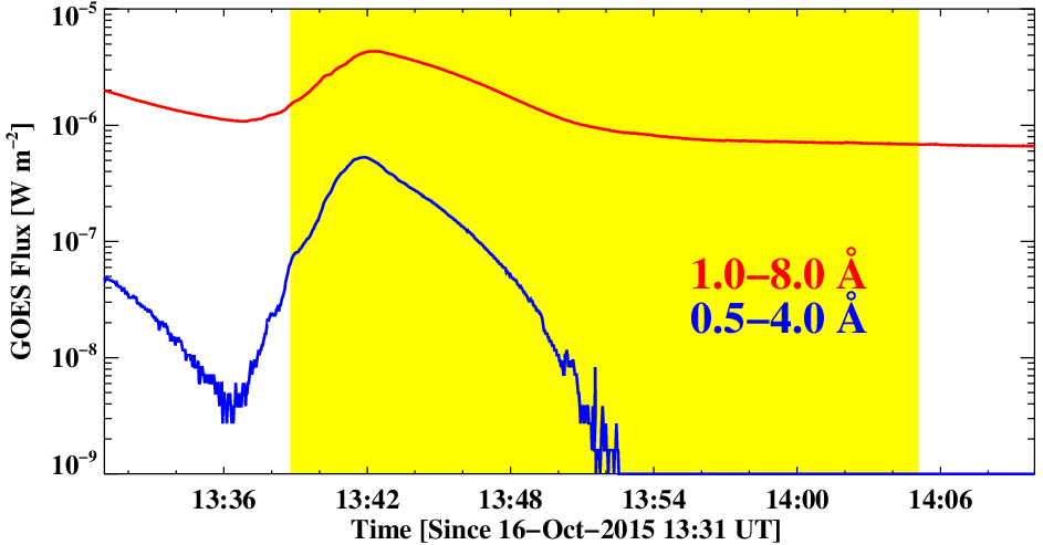
Figure 2 shows the SXR light curves of the flare in 18 Å (red line) and 0.54 Å (blue line). The SXR emissions started to increase at 13:36:30 UT and reached the peak values at 13:42:30 UT, before declining gradually until 13:51 UT (see also Fig. 5 in Paper I). The time of loop oscillation during 13:3914:05 UT is labeled with yellow area. It is found that the start time of transverse loop oscillation coincides with the fast ejection of jet (see also Fig. 4 in Paper I), and the oscillation covers part of the impulsive and whole decay phase of the flare, lasting for 26 min. The excitation of loop oscillation in our study can be interpreted by the schematic cartoon (Zimovets & Nakariakov 2015, see their Fig. 2).
To investigate the transverse loop oscillation, we choose three points along the loop: the first one is near the loop top, the third one is close to the southwest footpoint, and the second one in between. We place three artificial slices (S1, S2, and S3) across the points and just perpendicular to the loop, which are drawn with white solid lines in Fig. 1. The corresponding time-distance diagrams in 171 Å are plotted in the top three panels of Fig. 3. It is seen that excited by the jet, the loop deviated from the equilibrium state and began to move southward at 13:39 UT coherently. Then the loop moved backward and oscillated with decaying amplitude for more than three cycles. The almost identical phases of the transverse loop oscillation at different positions along the loop indicate that the oscillation belong to the standing fast kink mode.

To determine the parameters of kink oscillation along different slices, we mark the positions of the loop manually, which are connected with magenta dashed lines in Fig. 3. The kink oscillation is fitted with an exponentially decaying sine function (Nakariakov et al. 1999; Zhang et al. 2020) using the standard SSW program mpfit.pro:
| (4) |
where is the initial amplitude, is the period, is the damping time, is the initial phase, and is a linear term of the equilibrium position of the loop.
In Fig. 4, the green crosses represent the positions of the loop along the three slices in 171 and 131 Å, and the results of curve fitting are plotted with blue lines. It is obvious that the curve fitting using Equation 4 is satisfactory. The fitted parameters are listed in Table 1. In 171 Å, the initial amplitude decreases from 13.6 Mm near the loop top to 8.9 Mm near the footpoint. The period ranges from 440 s to 480 s with an average value of 462 s. The damping time ranges from 710 s to 1190 s with an average value of 976 s. The quality factor () lie in the range of 1.52.5. The oscillation decays much faster near the loop top than the loop leg. The parameters in 131 Å are close to those in 171 Å.

| (Mm) | (s) | (s) | ||
| 171 Å S1 | 13.60.3 | 4794 | 71426 | 1.50.1 |
| 171 Å S2 | 10.40.2 | 4672 | 118549 | 2.50.1 |
| 171 Å S3 | 8.90.3 | 4413 | 102955 | 2.30.1 |
| 131 Å S3 | 8.60.3 | 4353 | 109566 | 2.50.2 |
3.2 Magnetic field estimated from coronal seismology
As mentioned in Sect. 1, estimation of the magnetic field strength of oscillating loops is an important application of coronal seismology. To estimate the magnetic field of the large-scale coronal loop in Fig. 1, we consider the loop as a straight cylinder with the magnetic field lines frozen. The period of standing kink-mode oscillation depends on the loop length () and phase speed (Nakariakov et al. 1999):
| (5) |
where is the Alfvén speed in the loop, and and stand for the external and internal plasma densities.

In Fig. 1, the apparent distance between the footpoints of loop is 256, while the real distance becomes 268 after correcting the projection effect. Since there were no stereoscopic observations from the STEREO (Kaiser 2005) spacecrafts, the true geometry of the loop could not be inferred by stereoscopy. We assume a semi-elliptical shape of the loop initially in the -plane, which is determined by the major axis (2) and minor axis (2). The minor axis is taken to be the length of the loop baseline in spherical coordinates, while the major axis is varied. The loop is sequentially rotated around the , , and axes by angles of , , and , respectively. The projected loop in the -plane is then translated to compare with the observed loop in Fig. 1. By varying continuously the values of 2 and three rotation angles, we can find the best values of loop parameters when the average distance between the projected loop and the observed loop is minimized using mpfit.pro.
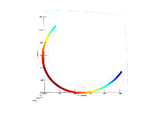
Figure 5 shows the three-dimensional (3D) geometry of the semi-elliptical loop, where , , , , and . In Fig. 6, the projected loop in the -plane is drawn with the blue solid line and the observed loop is drawn with the red dashed line. It is clear that the projected loop fits well with the observed loop, suggesting that the semi-elliptical shape can satisfactorily represent the true geometry of the oscillating loop. The length of the loop is calculated to be 377 Mm, which is 1.2 times longer than the value assuming a semicircular shape. Therefore, is estimated to be 1630 km s-1 by adopting an average period of oscillation ( s). is estimated to be 1210 km s-1 assuming that the density ratio is equal to 0.1 (Nakariakov et al. 1999; Nakariakov & Ofman 2001).
The Alfvén speed is determined by the magnetic field strength and mass density of the plasma. Consequently, we can estimate the magnetic field strength in the loop (Nakariakov & Ofman 2001):
| (6) |
where , is the proton mass, and is the LOS depth of the coronal loop. In Fig. 1(b), three tiny boxes, representing the loop top, loop leg, and loop footpoint, are used to perform DEM analysis described in Sect. 2.2. The inverted DEM profiles are displayed in Fig. 7(a-c), with the calculated values of and EM being labeled. The average temperature of the oscillating loop is 2 MK, which is consistent with the fact that the oscillation is observed in 131, 171, 193, and 211 Å. The background-subtracted intensity distribution of a short line (9.1 Mm in length) across the middle box is shown in Fig. 7(d). Single-Gauss fitting of the profile is used to derive the FWHM (3.4 Mm), which is considered as the width or LOS depth of the loop. Hence, the number density () and corresponding mass density () of the loop decrease from 6109 cm-3 and 110-14 g cm-3 near the footpoint to 2.9109 cm-3 and 4.810-15 g cm-3 near the loop top. The magnetic field strength of the loop () falls in the range of 3043 G according to Equation 6.

3.3 Magnetic field determined by NLFFF modeling
To validate the magnetic field strength of the oscillating loop inferred from coronal seismology, we carry out NLFFF modeling to construct magnetic field models by using the flux rope insertion method (van Ballegooijen 2004). We have briefly introduced the method in Sect. 2.3, and more details can be found in Bobra et al. 2008 and Su et al. 2009; Su et al. 2011.
The boundary condition for the high-resolution region is derived from the LOS magnetogram taken by HMI at 13:36 UT on 2015 October 16. The longitude-latitude map of the radial component of the magnetic field in the high-resolution region is presented in Fig. 8(b). Three flux ropes with the same poloidal flux (0 Mx cm-1) are inserted. However, the axial fluxes are different, namely, 81020 Mx, 11020 Mx and 41020 Mx, respectively. In Fig. 8(c), selected model field lines matching the observed non-potential coronal loops are overlaid on the AIA 171 Å image. In Fig. 8(d), the observed loop is traced manually and marked with the red line. In order to find the field line that best fit the observed loop, we first measure the distance between a point on the observed loop and the closest point on the projected field line in the image plane. These distances for various points along the observed loop are then averaged, which is defined as the “average deviation” (Su et al. 2009). The manually selected 3D field line that can minimize the deviation is considered as the line that best fits the observed loop (pink line), which is overlaid on the AIA 171 Å image. The length of the pink line (354 Mm) accounts for 94% of the loop length assuming a semi-elliptical shape. We obtained the magnetic field strength at several locations along the model field line, which lies in the range of 2123 G and is in the same order of magnitude as the result of coronal seismology.

4 Summary and Discussion
In this work, we report our multiwavelength observations of the transverse oscillation of a large-scale coronal loop induced by a blowout jet related to a C4.2 CRF in AR 12434 on 2015 October 16. The oscillation is most pronounced in AIA 171 and 131 Å. The oscillation is almost in phase along the loop with a peak initial amplitude of 13.6 Mm, meaning that the oscillation belong to the fast standing kink mode. The oscillation lasts for 3.5 cycles with an average period of 462 s and average damping time of 976 s. The values of lie in the range of 1.52.5. Based on coronal seismology, the Alfvén speed in the oscillating loop is estimated to be 1210 km s-1. Two independent approaches are applied to calculate the magnetic field strength of the loop, resulting in 3043 G using the coronal seismology and 2123 G using the NLFFF modeling. The results of two methods are in the same order of magnitude, which confirms the reliability of coronal seismology in diagnosing coronal magnetic field.
As mentioned in Sect. 1, transverse loop oscillations triggered by CRFs have been observed. Zhang et al. 2015 analyzed an M6.7 flare as a result of partial filament eruption on 2011 September 8. Kink oscillation was induced in an adjacent coronal loop within the same AR (see their Fig. 7). The oscillation with a small amplitude (1.6 Mm) lasted for 2 cycles without significant damping. The estimated parameters are listed and compared with this study in Table 2. It is found that the values of and are close to each other for the two events. Both the loop length and period in this study are 2 times larger than those for the event in 2011. However, the density and magnetic field of the loop in 2011 are much larger than those in our study. Zhang et al. 2020 investigated the decayless and decaying kink oscillations of an EUV loop on 2014 March 5. For comparison, the parameters, including the shortest loop length and period among the three events, are also listed in the last row of Table 2.
| Date | AR | Ref. | ||||||
| (s) | (Mm) | (km s-1) | (km s-1) | (109 cm-3) | (G) | |||
| 2011/09/08 | 11283 | 225 | 167 | 1482 | 1100 | 25 | 79 | Zhang et al. 2015 |
| 2015/10/16 | 12434 | 462 | 377 | 1630 | 1210 | 36 | 3043 | this study |
| 2014/03/05 | 11991 | 117 | 130 | 2200 | 1555 | 710 | 6578 | Zhang et al. 2020 |
Aschwanden & Schrijver 2011 compared the magnetic field of an oscillating loop determined by coronal seismology with the result of magnetic extrapolation based on the potential field source surface (PFSS) modeling using the photospheric magnetogram. It is found that the average extrapolated magnetic field strength exceeded the seismologically determined value (4 G) by a factor of two. After improving the method of estimation of physical parameters by taking the effect of density and magnetic stratification into account, the extrapolated magnetic field are optimized (Verwichte et al. 2013a). Guo et al. 2015 reported the kink oscillation of a coronal loop with a total length of 204 Mm, which was excited by the global fast magneto-acoustic wave as a result of flux rope eruption and the associated eruptive flare on 2013 April 11. Based on coronal seismology, they derived the spatial distribution of magnetic field (8 G) along the loop, which matches with that derived by a potential field model. Long et al. 2017 estimated the magnetic field of a trans-equatorial loop system using two independent techniques. It is found that the magnetic field strength (5.5 G) estimated by two approaches are roughly equal.
Acknowledgements.
The authors are grateful to the referee for valuable suggestions. The authors also appreciate Drs. Z. J. Ning, D. Li, and F. Chen for valuable discussions. SDO is a mission of NASA’s Living With a Star Program. AIA and HMI data are courtesy of the NASA/SDO science teams. Q.M.Z. is supported by the Science and Technology Development Fund of Macau (275/2017/A), CAS Key Laboratory of Solar Activity, National Astronomical Observatories (KLSA202006), Youth Innovation Promotion Association CAS, and the International Cooperation and Interchange Program (11961131002). This work is funded by NSFC grants (No. 11790302, 11790300, 11773079, 41761134088, 11473071, 12073081), and the Strategic Priority Research Program on Space Science, CAS (XDA15052200, XDA15320301).References
- Andries et al. (2009) Andries, J., van Doorsselaere, T., Roberts, B., et al. 2009, Space Sci. Rev., 149, 3
- Anfinogentov et al. (2013) Anfinogentov, S., Nisticò, G., & Nakariakov, V. M. 2013, A&A, 560, A107
- Antolin & Verwichte (2011) Antolin, P. & Verwichte, E. 2011, ApJ, 736, 121. doi:10.1088/0004-637X/736/2/121
- Arregui et al. (2007) Arregui, I., Andries, J., Van Doorsselaere, T., et al. 2007, A&A, 463, 333
- Aschwanden et al. (1999) Aschwanden, M. J., Fletcher, L., Schrijver, C. J., et al. 1999, ApJ, 520, 880
- Aschwanden et al. (2002) Aschwanden, M. J., de Pontieu, B., Schrijver, C. J., et al. 2002, Sol. Phys., 206, 99
- Aschwanden & Schrijver (2011) Aschwanden, M. J., & Schrijver, C. J. 2011, ApJ, 736, 102
- Aschwanden et al. (2013) Aschwanden, M. J., Boerner, P., Schrijver, C. J., et al. 2013, Sol. Phys., 283, 5. doi:10.1007/s11207-011-9876-5
- Bobra et al. (2008) Bobra, M. G., van Ballegooijen, A. A., & DeLuca, E. E. 2008, ApJ, 672, 1209
- Chen et al. (2019) Chen, X., Yan, Y., Tan, B., et al. 2019, ApJ, 878, 78
- Cheng et al. (2012) Cheng, X., Zhang, J., Saar, S. H., et al. 2012, ApJ, 761, 62
- Cheung et al. (2015) Cheung, M. C. M., Boerner, P., Schrijver, C. J., et al. 2015, ApJ, 807, 143
- Duckenfield et al. (2018) Duckenfield, T., Anfinogentov, S. A., Pascoe, D. J., et al. 2018, ApJ, 854, L5. doi:10.3847/2041-8213/aaaaeb
- Duckenfield et al. (2019) Duckenfield, T. J., Goddard, C. R., Pascoe, D. J., et al. 2019, A&A, 632, A64. doi:10.1051/0004-6361/201936822
- Edwin & Roberts (1983) Edwin, P. M., & Roberts, B. 1983, Sol. Phys., 88, 179
- Goddard et al. (2016) Goddard, C. R., Nisticò, G., Nakariakov, V. M., et al. 2016, A&A, 585, A137
- Goddard & Nakariakov (2016) Goddard, C. R., & Nakariakov, V. M. 2016, A&A, 590, L5
- Goossens et al. (2002) Goossens, M., Andries, J., & Aschwanden, M. J. 2002, A&A, 394, L39
- Goossens et al. (2008) Goossens, M., Arregui, I., Ballester, J. L., et al. 2008, A&A, 484, 851
- Guo et al. (2015) Guo, Y., Erdélyi, R., Srivastava, A. K., et al. 2015, ApJ, 799, 151
- Handy et al. (1999) Handy, B. N., Acton, L. W., Kankelborg, C. C., et al. 1999, Sol. Phys., 187, 229
- Hannah & Kontar (2012) Hannah, I. G. & Kontar, E. P. 2012, A&A, 539, A146
- Kaiser (2005) Kaiser, M. L. 2005, Advances in Space Research, 36, 1483. doi:10.1016/j.asr.2004.12.066
- Lee et al. (2020) Lee, J., White, S. M., Chen, X., et al. 2020, ApJ, 901, L10. doi:10.3847/2041-8213/abb4dd
- Lemen et al. (2012) Lemen, J., Title, A., Akin, D., et al. 2012, Sol. Phys., 275, 17
- Li et al. (2017) Li, D., Ning, Z. J., Huang, Y., et al. 2017, ApJ, 849, 113
- Li et al. (2018a) Li, D., Yuan, D., Su, Y. N., et al. 2018a, A&A, 617, A86
- Li et al. (2018b) Li, T., Yang, S., Zhang, Q., et al. 2018b, ApJ, 859, 122
- Liu et al. (2020) Liu, C., Prasad, A., Lee, J., et al. 2020, ApJ, 899, 34
- Long et al. (2017) Long, D. M., Valori, G., Pérez-Suárez, D., et al. 2017, A&A, 603, A101
- Masson et al. (2009) Masson, S., Pariat, E., Aulanier, G., et al. 2009, ApJ, 700, 559
- Morgan & Pickering (2019) Morgan, H. & Pickering, J. 2019, Sol. Phys., 294, 135
- Nakariakov et al. (1999) Nakariakov, V. M., Ofman, L., Deluca, E. E., et al. 1999, Science, 285, 862
- Nakariakov & Ofman (2001) Nakariakov, V. M., & Ofman, L. 2001, A&A, 372, L53
- Nakariakov & Verwichte (2005) Nakariakov, V. M., & Verwichte, E. 2005, Living Reviews in Solar Physics, 2, 3
- Nechaeva et al. (2019) Nechaeva, A., Zimovets, I. V., Nakariakov, V. M., et al. 2019, ApJS, 241, 31. doi:10.3847/1538-4365/ab0e86
- Nisticò et al. (2013) Nisticò, G., Nakariakov, V. M., & Verwichte, E. 2013, A&A, 552, A57
- Nisticò et al. (2017) Nisticò, G., Polito, V., Nakariakov, V. M., et al. 2017, A&A, 600, A37
- Ofman & Aschwanden (2002) Ofman, L. & Aschwanden, M. J. 2002, ApJ, 576, L153. doi:10.1086/343886
- Pascoe et al. (2016) Pascoe, D. J., Goddard, C. R., Nisticò, G., et al. 2016, A&A, 585, L6
- Pesnell et al. (2012) Pesnell, W., Thompson, B., & Chamberlin, P. 2012, Sol. Phys., 275, 3
- Plowman et al. (2013) Plowman, J., Kankelborg, C., & Martens, P. 2013, ApJ, 771, 2
- Ruderman & Roberts (2002) Ruderman, M. S., & Roberts, B. 2002, ApJ, 577, 475
- Ruderman & Erdélyi (2009) Ruderman, M. S., & Erdélyi, R. 2009, Space Sci. Rev., 149, 199
- Schou et al. (2012) Schou, J., Scherrer, P., Bush, R., et al. 2012, Sol. Phys., 275, 229
- Schrijver et al. (2002) Schrijver, C. J., Aschwanden, M. J., & Title, A. M. 2002, Sol. Phys., 206, 69
- Su et al. (2009) Su, Y., van Ballegooijen, A., Lites, B. W., et al. 2009, ApJ, 691, 105
- Su et al. (2011) Su, Y., Surges, V., van Ballegooijen, A., et al. 2011, ApJ, 734, 53
- Su et al. (2015) Su, Y., van Ballegooijen, A., McCauley, P., et al. 2015, ApJ, 807, 144
- Su et al. (2018a) Su, Y., Liu, R., Li, S., et al. 2018a, ApJ, 855, 77
- Su et al. (2018b) Su, Y., Veronig, A. M., Hannah, I. G., et al. 2018b, ApJ, 856, L17. doi:10.3847/2041-8213/aab436
- Su (2019) Su, Y. N. 2019, Acta Astronomica Sinica, 60, 2
- van Ballegooijen (2004) van Ballegooijen, A. A. 2004, ApJ, 612, 519
- Van Doorsselaere et al. (2008) Van Doorsselaere, T., Nakariakov, V. M., Young, P. R., et al. 2008, A&A, 487, L17
- Verwichte et al. (2006) Verwichte, E., Foullon, C., & Nakariakov, V. M. 2006, A&A, 452, 615
- Verwichte et al. (2013a) Verwichte, E., Van Doorsselaere, T., Foullon, C., et al. 2013a, ApJ, 767, 16
- Verwichte et al. (2013b) Verwichte, E., Van Doorsselaere, T., White, R. S., et al. 2013b, A&A, 552, A138
- Weber et al. (2004) Weber, M. A., Deluca, E. E., Golub, L., et al. 2004, Multi-wavelength Investigations of Solar Activity, 321
- White & Verwichte (2012) White, R. S., & Verwichte, E. 2012, A&A, 537, A49
- Yang et al. (1986) Yang, W. H., Sturrock, P. A., & Antiochos, S. K. 1986, ApJ, 309, 383
- Yuan & Van Doorsselaere (2016) Yuan, D., & Van Doorsselaere, T. 2016, ApJS, 223, 24
- Zhang & Ji (2014) Zhang, Q. M., & Ji, H. S. 2014, A&A, 567, A11
- Zhang et al. (2015) Zhang, Q. M., Ning, Z. J., Guo, Y., et al. 2015, ApJ, 805, 4
- Zhang et al. (2016a) Zhang, Q. M., Ji, H. S., & Su, Y. N. 2016a, Sol. Phys., 291, 859
- Zhang et al. (2016b) Zhang, Q. M., Li, D., & Ning, Z. J. 2016b, ApJ, 832, 65
- Zhang et al. (2016c) Zhang, Q. M., Li, D., Ning, Z. J., et al. 2016c, ApJ, 827, 27. doi:10.3847/0004-637X/827/1/27
- Zhang et al. (2019) Zhang, Q. M., Cheng, J. X., Feng, L., et al. 2019, ApJ, 883, 124
- Zhang et al. (2020) Zhang, Q. M., Dai, J., Xu, Z., et al. 2020, A&A, 638, A32
- Zhang (2020) Zhang, Q. M. 2020, A&A, 642, A159. doi:10.1051/0004-6361/202038557
- Zimovets & Nakariakov (2015) Zimovets, I. V., & Nakariakov, V. M. 2015, A&A, 577, A4