Algebraic Weaves and Braid Varieties

Roger Casals Address: Dept. of Mathematics
University of California, Davis
One Shields Avenue, Davis, CA 95616 Email address: casals@math.ucdavis.edu , Eugene Gorsky Address: Dept. of Mathematics
University of California, Davis
One Shields Avenue, Davis, CA 95616 Email address: egorskiy@math.ucdavis.edu , Mikhail Gorsky Address: Department of Mathematics, University of Vienna, Oscar-Morgenstern Platz 1, 1090 Vienna, Austria Email address: mikhail.gorskii@univie.ac.at and José Simental Address: Instituto de Matemáticas
Universidad Nacional Autónoma de México
Ciudad Universitaria, Mexico City, Mexico 04510 Email address: simental@im.unam.mx

Abstract.

In this manuscript we study braid varieties, a class of affine algebraic varieties associated to positive braids. Several geometric constructions are presented, including certain torus actions on braid varieties and holomorphic symplectic structures on their respective quotients. We also develop a diagrammatic calculus for correspondences between braid varieties and use these correspondences to obtain interesting decompositions of braid varieties and their quotients. It is shown that the maximal charts of these decompositions are exponential Darboux charts for the holomorphic symplectic structures, and we relate these charts to exact Lagrangian fillings of Legendrian links.

2010 Mathematics Subject Classification

Primary: 53D10. Secondary: 53D15, 57R17.

1. Introduction

This article studies braid varieties, a class of affine algebraic varieties associated to positive braids, and their relation to contact and symplectic geometry. First, the geometric properties of braid varieties are studied, including the construction of torus actions and holomorphic symplectic structures on their quotients. Then, we construct correspondences between these braid varieties by using certain moduli spaces associated to weaves, a class of labeled planar diagrams. These geometric correspondences are shown to induce valuable decompositions for braid varieties and their quotients, also unifying known constructions of P. Boalch and A. Mellit, in the case of character varieties, and M. Henry and D. Rutherford, in the case of augmentation varieties.

The diagrammatic calculus based on weaves, presented in Section 5, allows for direct and explicit computations, and we provide new constructions of embedded exact Lagrangian fillings for Legendrian links through combinatorial methods. The main results of the article are Theorems 1.1, 1.3 and 1.7, and several detailed examples are provided throughout the manuscript. In particular, we believe that the construction of a holomorphic symplectic structure on augmentation varieties, developed in Section 3 is of value for contact and symplectic geometry.

1.1. Context

Legendrian links in contact 3–manifolds [1, 4, 48] are central in contact and symplectic geometry. Legendrian fronts, immersed planar cuspidal curves, arise in topology, as Cerf diagrams [2, 11, 28], in differential equations, as Stokes data for irregular singularities [5, 102, 104], and in analysis, as wavefront sets [60, 61, 74]. In this article, we use that a positive braid $\beta$ gives rise to a Legendrian link $\Lambda(\beta)\subseteq(\mathbb{R}^{3},\xi_{\text{st}})$ , cf. [23, Section 2.2] or [17, 48].

Associated to a Legendrian link $\Lambda\subseteq(\mathbb{R}^{3},\xi_{\text{st}})$ , there exist two geometrically defined moduli spaces: the moduli space of microlocal sheaves in $\mathbb{R}^{2}$ microlocally supported at $\Lambda$ , cf. [24, 55, 68, 69], and the moduli space of exact Lagrangian fillings $L\subseteq(\mathbb{R}^{4},\omega_{\text{st}})$ , with boundary $\partial L=\Lambda$ , cf. [2, 17, 23, 48]. Note that the latter can be understood as the (geometric part of the) moduli space of objects of the Fukaya category of $(\mathbb{R}^{4},\omega_{\text{st}})$ partially wrapped at $\Lambda$ . For the Legendrian links $\Lambda(\beta)\subseteq(\mathbb{R}^{3},\xi_{\text{st}})$ , these moduli are algebraic stacks and, when appropriately decorated, smooth algebraic varieties. The present manuscript studies a collection of algebraic varieties associated to a positive braid $\beta$ , including and generalizing these two moduli spaces, and new correspondences between them. These algebraic correspondences are often induced by geometric exact Lagrangian cobordisms between Legendrian links, and can in general be described with a diagrammatic calculus, as we will show, building on work of the first author with E. Zaslow [25].

In summary, we introduce the class of braid varieties, study torus actions and their quotients, construct correspondences and morphisms between them, and develop a diagrammatic calculus associated to these correspondences. As we establish these results, we prove several theorems of interest, including the fact that the augmentation variety associated to $\Lambda(\beta)$ admits a holomorphic symplectic structure, and explain the relation between A. Mellit’s decomposition of character varieties [82] and the ruling stratification of the augmentation variety [56, 57]. Note that holomorphic symplectic structures play a central role in the study of moduli spaces of connections [7, 9], and there ought to be a relation to their symplectic structures through understanding the moduli stack of objects in the $\mbox{Aug}_{+}$ -category [86] as a wild character variety [6, 101]. It should be noted that our diagrammatic calculus, which we refer to as algebraic weaves, provides a combinatorial and explicit approach to these decompositions. In addition, the pieces are compatible with the holomorphic symplectic structure, the open toric charts admitting (exponential) holomorphic Darboux coordinates.

1.2. Main Results

Let us define our main object of study, the braid matrices and braid varieties. In order to do this, let us fix $n>0$ . For each $i=1,\dots,n-1$ , we consider the braid matrix $B_{i}(z)\in\operatorname{GL}(n,\mathbb{C}[z])$ defined by:

(B_{i}(z))_{jk}:=\begin{cases}1&j=k\text{ and }j\neq i,i+1\\ 1&(j,k)=(i,i+1)\text{ or }(i+1,i)\\ z&j=k=i+1\\ 0&\text{otherwise;}\end{cases},\qquad\mbox{i.e.}\quad B_{i}(z):=\left(\begin{matrix}1&\cdots&&&\cdots&0\\ \vdots&\ddots&&&&\vdots\\ 0&\cdots&0&1&\cdots&0\\ 0&\cdots&1&z&\cdots&0\\ \vdots&&&&\ddots&\vdots\\ 0&\cdots&&&\cdots&1\\ \end{matrix}\right).

Note that the only the non-trivial $(2\times 2)$ -block is at $i$ th and $(i+1)$ st rows. Braid matrices have appeared in a range of areas, starting with L. Euler’s continuants [40], G. Stokes’ study of irregular singularities [104] (see P. Boalch’s [8, 9]), M. Broué and J. Michel’s work on Deligne-Lusztig varieties [12], P. Deligne’s braid invariants [30], and more recently in T. Kálmán’s study of the Legendrian Contact DGA [66] (see also [23]) and A. Mellit’s results on the curious Lefschetz property for character varieties [82], among others.

Let $\gamma$ be a positive $n$ -braid word $[\gamma]\in\mathrm{Br}^{+}_{n}$ , $\gamma=\sigma_{i_{1}}\cdots\sigma_{i_{\ell}}$ . We consider the following matrix $B_{\gamma}(z_{1},\ldots,z_{\ell})\in\operatorname{GL}(n,\mathbb{C}[z_{1},\ldots,z_{\ell}])$ , we which define to be the matrix product

B_{\gamma}(z_{1},\ldots,z_{\ell}):=B_{i_{1}}(z_{1})\cdots B_{i_{\ell}}(z_{\ell}).

Finally, if $\pi\in\operatorname{GL}(n,\mathbb{C})$ is a permutation matrix we consider the braid variety

X_{0}(\gamma;\pi):=\left\{(z_{1},\ldots,z_{\ell})\ :\ B_{\gamma}(z_{1},\ldots,z_{\ell})\pi\ \text{is upper-triangular}\right\}\subseteq\mathbb{C}^{\ell}.

Note that this is an affine algebraic variety, given by the vanishing of $\binom{n}{2}$ polynomial equations in the variables $z_{1},\dots,z_{\ell}$ .

From our definition above, it is simple to see that $X_{0}(\gamma;\pi)$ is isomorphic to $X_{0}(\gamma^{\prime};\pi)$ if $[\gamma]=[\gamma^{\prime}]\in\mathrm{Br}_{n}$ , i.e. if two positive words $\gamma,\gamma^{\prime}$ represent the same $n$ -braid, the resulting braid varieties are isomorphic, hence the name. In the course of the article, the permutation (matrix) $\pi$ will often be the identity $\pi=\mathrm{Id}=e\in S_{n}$ or the longest element $\pi=w_{0}=(n\ n-1\ \ldots\ 1)\in S_{n}$ . Let $\Delta\in\mathrm{Br}^{+}_{n}$ be a positive braid lift of the permutation $w_{0}$ , i.e. $\Delta$ will be a braid word for the half-twist. See Example 2.2 for our specific choice of positive braid word for $\Delta$ .

The first result of the article establishes geometric properties of braid varieties, including the existence of a torus action and their relation to the Floer-theoretically defined augmentation varieties [10, 27, 86]. It reads as follows.

Theorem 1.1.

Let $\gamma$ be a positive $n$ -braid word $[\gamma]\in\mathrm{Br}^{+}_{n}$ . Then the following statements hold:

(i)

$X_{0}(\gamma\Delta;1)\simeq X_{0}(\gamma;w_{0})\times\mathbb{C}^{\binom{n}{2}}$ , and $X_{0}(\gamma;w_{0})$ is non-empty if and only if the Demazure product of $\gamma$ equals $w_{0}$ . In this case, $X_{0}(\gamma;w_{0})$ is an irreducible complete intersection of dimension $\ell(\gamma)-\binom{n}{2}$ , and $X_{0}(\gamma\Delta;1)$ is an irreducible complete intersection of dimension $\ell(\gamma)$ .

Suppose that there exists a positive $n$ -braid word $\beta$ such that $\gamma=\beta\Delta$ . Then:
(ii)

The braid variety $X_{0}(\beta\Delta;w_{0})$ , and thus $X_{0}(\beta\Delta^{2};1)$ , is smooth.
(iii)

There exists a free torus action on $X_{0}(\beta\Delta;w_{0})$ such that the quotient algebraic variety $X_{0}(\beta\Delta;w_{0})/T$ is smooth and holomorphic symplectic.
(iv)

There exists an isomorphism between $X_{0}(\beta\Delta;w_{0})/T$ and an augmentation variety $\operatorname{Aug}(\beta)$ associated to the Legendrian link $\Lambda(\beta)$ . In particular, $\operatorname{Aug}(\beta)$ is a holomorphic symplectic $($ smooth $)$ affine variety.
(v)

The open Bott-Samelson variety $\OBS(\beta)$ associated to $\beta$ is isomorphic to the quotient

$\OBS(\beta)\cong\left(\operatorname{GL}(n,\mathbb{C})\times X_{0}(\beta;1)\right)/\mathcal{B},$

where $\mathcal{B}\subseteq\operatorname{GL}(n,\mathbb{C})$ is the Borel subgroup of upper-triangular matrices.

In Theorem 1.1.(iii), the dimension of the torus $T$ does depend on the number of components in the closure of $\beta$ , see Section 2 for details. See Section 2.6 for the details on marked points used to define the objects in 1.1.(iv). The different varieties and the torus action featured in Theorem 1.1 are presented in the course of the article, and the proof of this theorem is obtained by gathering some the results we develop, such as Theorem 2.39, Theorem 2.6, Theorem 3.14 and Corollary 5.36. See also Section 4.4 for the definition of Demazure product, and note that the Demazure product of $\beta\Delta$ equals $w_{0}$ for any $\beta$ .

Theorem 1.1 discusses the absolute aspects of braid varieties. The study of such varieties also relies crucially on their relative geometry: morphisms between different such braid varieties and, more generally, correspondences, yield interesting (and useful) results. In order to study this relative setting, we develop the diagrammatic calculus of weaves, which we summarize as follows.

Let $\mathfrak{W}_{n}$ be the category defined as:

-

Objects: $\mbox{Ob}(\mathfrak{W}_{n})$ are arbitrary positive braid words $\gamma=\sigma_{i_{1}}\cdots\sigma_{i_{\ell}}$ , $[\gamma]\in Br^{+}_{n}$ ,

Morphisms: $\mbox{Hom}_{\mathfrak{W}_{n}}(\gamma,\gamma^{\prime})$ are compositions of the following six elementary moves, starting at $\gamma$ at the top and ending at $\gamma^{\prime}$ at the bottom. The moves are

\sigma_{i}\sigma_{i}\rightarrow\sigma_{i},\qquad\sigma_{i}\sigma_{i+1}\sigma_{i}\leftrightarrow\sigma_{i+1}\sigma_{i}\sigma_{i+1},\qquad\sigma_{i}\sigma_{j}\rightarrow\sigma_{j}\sigma_{i}\ (|i-j|>1),\quad\mbox{ and }\quad\sigma_{i}\sigma_{i}\leftrightarrow 1.

We will declare some of the morphisms to be equivalent, see section 4.

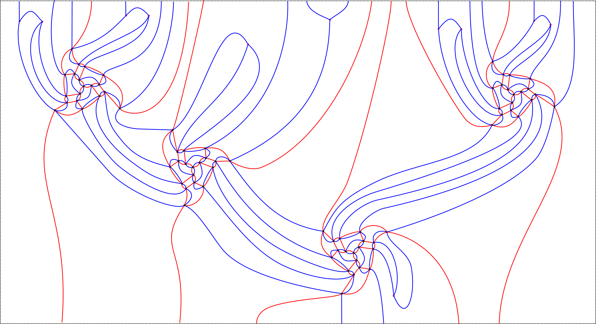
The morphisms in $\mathfrak{W}_{n}$ will be represented diagrammatically as certain planar graphs with edges decorated by simple transpositions $s_{i}$ . (Namely, $s_{i}$ are the Coxeter projections of the Artin braid generators $\sigma_{i}$ , $1\leq i\leq n$ .) These planar graphs are referred to as weaves, following [25, Section 2], and $\mathfrak{W}_{n}$ will be called the category of weaves. The elementary moves above, i.e. the building blocks for morphisms, can be drawn as follows:

There is also a dual 6-valent vertex corresponding to $\sigma_{i}\sigma_{i-1}\sigma_{i}\to\sigma_{i-1}\sigma_{i}\sigma_{i-1}$ which we do not draw here but is equally allowed. An algebraic weave, obtained by vertically and horizontally concatenating the models above (plus additional decorations), represents a morphism from the braid word on the top to the braid word on the bottom. The composition of weaves

\mbox{Hom}_{\mathfrak{W}_{n}}(\gamma^{\prime},\gamma^{\prime\prime})\times\mbox{Hom}_{\mathfrak{W}_{n}}(\gamma,\gamma^{\prime})\longrightarrow\mbox{Hom}_{\mathfrak{W}_{n}}(\gamma,\gamma^{\prime\prime})

is given by vertical stacking of these weave diagrams. See Figure 1 for an instance of a morphism.

Refer to caption — Figure 1. An algebraic weave in $\mbox{Hom}_{\mathfrak{W}_{n}}(\gamma,\gamma^{\prime})$ between the two positive $3$ -braids $\gamma=\sigma_{1}^{3}\sigma_{2}\sigma_{1}^{3}\sigma_{1}^{2}\sigma_{1}^{3}\sigma_{2}^{3}\sigma_{1}^{3}\sigma_{2}\sigma_{1}^{3}$ , at the top, and $\gamma^{\prime}=\sigma_{2}^{3}\sigma_{1}^{2}\sigma_{2}^{2}$ , at the bottom. The color code is that blue is labeled with the transposition $s_{1}$ and red is labeled with $s_{2}$ . For readability we omit the (downward pointing) orientations. The upside-down trivalent vertices are defined using the usual trivalent vertices and cups, see Section 4.3.2.

Remark 1.2.

Note that this diagrammatic category is in part similar to the categories appearing in Soergel calculus [37, 38], but differs in several key aspects. In particular, in the category of algebraic weaves there is no requirement that the two ways of getting from $\sigma_{i}\sigma_{i}\sigma_{i}$ to $\sigma_{i}$ , via the moves $\sigma_{i}\sigma_{i}\rightarrow\sigma_{i}$ , are equivalent:

The difference between these diagrams will be referred to as a weave mutation.

Let $\mathfrak{C}$ be the category of algebraic varieties whose morphisms are correspondences. That is, a morphism $X\to Y$ consists of a pair of morphisms $X\leftarrow Z\rightarrow Y$ , and composition corresponds to the fiber product. The second result in this manuscript shows that braid varieties and their correspondences provide a realization of the weave category $\mathfrak{W}_{n}$ , as follows.

Theorem 1.3.

There exists a functor $\mathfrak{X}_{0}:\mathfrak{W}_{n}\longrightarrow\mathfrak{C}$ such that:

(a)

Objects: For a positive braid word $\gamma\in\mbox{Ob}(\mathfrak{W}_{n})$ , the functor $\mathfrak{X}_{0}$ associates the braid variety $\mathfrak{X}_{0}(\gamma):=X_{0}(\beta;w_{0})$ .
(b)

Morphisms: For a weave $\mathfrak{w}\in\mathrm{Hom}_{\mathfrak{W}_{n}}(\beta_{2},\beta_{1})$ , the functor associates a correspondence $\mathfrak{X}_{0}(\mathfrak{w})$ between $X_{0}(\beta_{2};w_{0})$ and $X_{0}(\beta_{1};w_{0})$ , such that correspondences $\mathfrak{X}_{0}(\mathfrak{w})$ and $\mathfrak{X}_{0}(\mathfrak{w}^{\prime})$ associated to equivalent weaves with no caps $\mathfrak{w},\mathfrak{w}^{\prime}$ are isomorphic. $($ The algebraic variety $\mathfrak{X}_{0}(\mathfrak{w})$ is in fact described as a certain moduli space governed by the weave $\mathfrak{w}$ . $)$
(c)

Composition: Let $\mathfrak{w}_{1}\in\mathrm{Hom}_{\mathfrak{W}_{n}}(\beta_{1},\beta_{0})$ , $\mathfrak{w}_{2}\in\mathrm{Hom}_{\mathfrak{W}_{n}}(\beta_{2},\beta_{1})$ , and consider their composition $\mathfrak{w}=\mathfrak{w}_{1}\circ\mathfrak{w}_{2}\in\mathrm{Hom}_{\mathfrak{W}_{n}}(\beta_{2},\beta_{0})$ , which is obtained by vertical concatenation of $\mathfrak{w}_{2}$ , at the top, and $\mathfrak{w}_{1}$ , at the bottom. Then the composition of weaves under $\mathfrak{X}_{0}$ corresponds to the diagram:

where the middle square is Cartesian.

(d)

Let $\mathfrak{w}\in\mathrm{Hom}_{\mathfrak{W}_{n}}(\beta_{2},\beta_{1})$ be a weave with no caps, $a$ cups and $b$ trivalent vertices. Then the correspondence $\mathfrak{X}_{0}(\mathfrak{w})$ defines an injective map

\mathfrak{X}_{0}(\mathfrak{w}):\mathbb{C}^{a}\times(\mathbb{C}^{*})^{b}\times X_{0}(\beta_{1};w_{0})\hookrightarrow X_{0}(\beta_{2};w_{0}).

Furthermore, the correspondences $\mathfrak{X}_{0}(\mathfrak{w})$ are equivariant with respect to appropriate torus actions and, using Theorem 1.1. $($ iv $)$ , yield correspondences between augmentation varieties.

The proof of Theorem 1.3 occupies the majority of Section 5, the equivariance statement being discussed in Subsection 5.7. The statements in Theorem 1.3.(a)-(c) are the algebraic analogues of the symplectic geometric results obtained in [25]. Note that the algebraic variety $X_{0}(\Delta;w_{0})$ is a point, and thus Theorem 1.3 implies the following.

Corollary 1.4.

Let $\mathfrak{w}\in\mathrm{Hom}_{\mathfrak{W}_{n}}(\gamma,\Delta)$ be a weave with no caps, $a$ cups and $b$ trivalent vertices, $a,b\in\mathbb{N}$ . Then the correspondence $\mathfrak{X}_{0}(\mathfrak{w})$ yields an injective map

\mathfrak{X}_{0}(\mathfrak{w}):\mathbb{C}^{a}\times(\mathbb{C}^{*})^{b}\hookrightarrow X_{0}(\gamma;w_{0}),\ 2a+b=\ell(\gamma)-\binom{n}{2}.

Corollary 1.4 provides a unifying framework for many known decompositions, including the ruling stratification in augmentation varieties [43, 56, 57], and the decomposition by walks in character varieties [82]. First, we will see that any weave $\mathfrak{w}\in\mathrm{Hom}_{\mathfrak{W}_{n}}(\gamma,\Delta)$ with no cups or caps yields an open (algebraic) torus $(\mathbb{C}^{*})^{\ell(\gamma)-\binom{n}{2}}\subset X_{0}(\gamma;w_{0})$ . Fixing such a weave, we will see that its complement can be further decomposed with weaves (that will now include cups). The weaves with no caps or cups, that will be of primary importance in this article, will be referred to as Demazure weaves. Note that different Demazure weaves define (a priori) different decompositions of $X_{0}(\gamma;w_{0})$ .

Remark 1.5.

The manuscript also includes a new construction of weaves, coming from a class of labeled triangulations. This construction, described in Section 4.7, uses Demazure products in a crucial manner and, together with results of [25], provides a systematic (and combinatorial) mechanism to construct embedded exact Lagrangian fillings for Legendrian links in $(\mathbb{R}^{3},\xi_{\text{st}})$ which are obtained as closures of a positive braid $\beta$ . Specifically, the points in the braid variety $X_{0}(\beta;w_{0})$ correspond to fillings of the $(-1)$ -closure of $\beta\Delta$ , cf. [23, Section 2].

Finally, complementing Theorem 1.1 and Theorem 1.3, we give a geometric interpretation to these toric charts associated to Demazure weaves $\mathfrak{w}\in\mbox{Hom}_{\mathfrak{W}_{n}}(\beta\Delta,\Delta)$ , as follows.

First, we show in Section 2.3 that these charts can be combinatorially obtained by opening the crossings of the positive braid $\beta$ . Indeed, Section 2.3 shows that there is an injective map

X_{0}(\beta^{\prime}\Delta;w_{0})\times\mathbb{C}^{*}\hookrightarrow X_{0}(\beta\Delta;w_{0}),

if the positive braid word $\beta^{\prime}$ is obtained from $\beta$ by removing exactly one crossing. Therefore, opening the crossings in $\beta$ one by one, in some order, yields a toric chart in $X_{0}(\beta\Delta;w_{0})$ . Different orders might yield identical or different toric charts. For instance, for a 2-strand braid $\beta=\sigma_{1}^{n}$ , there are $n!$ possible orderings and one obtains a Catalan number $C_{n}$ of toric charts. In particular, in this correspondence, each toric chart is obtained by exactly one 312-pattern avoiding permutation.

Definition 1.6.

Throughout the paper, if $\beta$ is a braid word of length $\ell$ , we denote by $S_{\ell}$ the set of orderings on the crossings of $\beta$ (which is in bijection with the symmetric group in $\ell$ letters).

Regarding this relation, between toric charts and openings of crossings, we show the following.

Theorem 1.7.

Let $[\beta]\in Br^{+}_{n}$ be a positive braid and $\beta=\sigma_{i_{1}}\cdot\sigma_{i_{2}}\cdot\ldots\cdot\sigma_{i_{l}}$ a positive braid word. Consider an ordering $\rho\in S_{l}$ for the crossings of $\beta$ . Then:

(i)

There exists a $($ Demazure $)$ weave $\mathfrak{w}_{\rho}$ such that the sequence of crossing openings according to $\rho$ is realized by the weave $\mathfrak{w}_{\rho}$ . Conversely, any Demazure weave $\mathfrak{w}$ is equivalent to opening crossings for some ordering $\rho\in S_{l}$ , i.e. there exists $\rho\in S_{l}$ such that $\mathfrak{w}$ is equivalent to $\mathfrak{w}_{\rho}$ .
(ii)

Two toric charts $C_{1},C_{2}\subseteq X_{0}(\beta\Delta;w_{0})$ associated to different orderings of the crossings are represented by weaves $\mathfrak{w}_{1},\mathfrak{w}_{2}$ such that $\mathfrak{w}_{1},\mathfrak{w}_{2}$ are related by a sequence of mutations. In addition, the union of all such toric charts covers $X_{0}(\beta\Delta;w_{0})$ up to codimension 2.

The first item is proven in Lemma 5.17 and Theorem 5.18, and the proof of the codimension-2 cover is established in Theorem 2.25. The mutation equivalence of any weaves yielding toric charts follows from the more general Theorem 4.12, which states that, under technical conditions that are satisfied in the weaves pertaining to Theorem 1.7, any two Demazure weaves between the same two braid words are related by a sequence of equivalence moves and mutations. Note that Theorem 4.12 is a translation of a result of B. Elias [36] to our weaves framework.

Remark 1.8.

Note that both the openings of crossings and mutations can be described in terms of braid words. Indeed, consider a braid word $\sigma_{i}u\sigma_{j}$ with $\sigma_{i}u=u\sigma_{j}$ , i.e. $(\sigma_{i},\sigma_{j})$ is a deletion pair in the notation of [58]. Then, we can consider two different weaves:

In this diagram, the left weave $\sigma_{i}u\sigma_{j}\to u\sigma_{j}$ corresponds to the opening of a crossing $\sigma_{i}$ , and the right weave $\sigma_{i}u\sigma_{j}\to u\sigma_{j}$ to opening a crossing $\sigma_{i}$ . Theorem 1.7 implies that the two weaves are always related by a sequence of equivalence moves and mutations. For example, for $i=j$ and $u=\sigma_{i}$ we get a mutation, while for $i=1,j=2$ and $u=\sigma_{2}\sigma_{1}$ we get an equivalence (see Section 4.2.4):

1.3. Related developments

In this section we comment on some recent results and developments which were completed after the first version of this paper was posted on arXiv.

We further studied certain classes braid varieties in [18]. In particular, all positroid varieties [71] in the Grassmannian $\mathrm{Gr}(k,n)$ were shown to be isomorphic to braid varieties for several different braids, both on $n$ and on $k$ strands. The paper [18] also gives a precise relation between braid varieties, subword complexes and brick polytopes [13, 26, 39, 52, 53, 63, 72, 73, 92]. The faces of a subword complex for a braid word $\gamma$ correspond to all possible subwords of $\gamma$ such that the Demazure product of their complements equals $w_{0}$ . Subword complexes were introduced by Knutson and Miller [72, 73] in the context of Gröbner geometry of Schubert polynomials. Knutson and Miller proved that subword complexes are homeomorphic to balls or spheres. Pilaud and Stump found polytopal realizations of spherical subword complexes and called them brick polytopes. Results of [52, 53, 54] describe the behavior of subword complexes under braid moves and moves $s_{i}s_{i}\to s_{i}$ in $\gamma$ . Ceballos, Labbé and Stump [26] proved that certain brick polytopes are generalized associahedra, thus relating subword complexes to the theory of cluster algebras. See also more recent works of Brodsky and Stump [13] and of Jahn, Löwe and Stump [63] further exploring this relation. Using the work of Escobar [39], we also show in [18] that a braid variety admits a smooth compactification by the so-called brick manifold. The combinatorics of the boundary divisor agree with the dual subword complex.

Finally, there was a recent increase of interest relating weaves, braid varieties and cluster algebras. In particular, in a joint work with I. Le and L. Shen [19], we show that any braid variety admits a cluster structure. This result was also proven in [45, 46, 98] by different methods, and we expect the two cluster structures to be closely related. The above results resolve a long-standing conjecture of Leclerc [76] on the existence of cluster structure on open Richardson varieties. In particular, a cluster structure guarantees the existence of a collection of open tori which correspond to Demazure weaves as in Corollary 1.4. On such a torus, [19] defines a collection of cluster coordinates using the combinatorics of a weave. We refer to [19, 45, 46, 98, 99, 100] and references therein for all definitions and details.

Acknowledgements: This paper started as a joint project with our colleague Monica Vazirani, and would not have happened without her; we thank her warmly. We also thank Ben Elias, Honghao Gao, Tamas Kálmán, Anton Mellit, Lenny Ng, Minh-Tam Trinh and Daping Weng for useful discussions, and Johan Asplund for comments on an earlier version of the paper. E. Gorsky would like to thank Yuri Chekanov for the lifetime influence. We would like to thank the anonymous referee for their very thorough reading of the paper and many helpful suggestions.

R. Casals is supported by the NSF grant DMS-1841913, the NSF CAREER grant DMS-1942363, the Alfred P. Sloan Foundation and a UC Davis College of L&S Dean’s Fellowship. The work of E. Gorsky was partially supported by the NSF grants DMS-1700814, DMS-1760329 and DMS-2302305. Parts of this work were done when M. Gorsky’s participated in the junior trimester program “New Trends in Representation Theory” at the Hausdorff Institute for Mathematics in Bonn. M. Gorsky was partially supported by the French ANR grant CHARMS (ANR-19-CE40-0017) and received funding from the European Research Council (ERC) under the European Union’s Horizon 2020 research and innovation programme (grant agreement No. 101001159). J.S. was partially supported by CONAHCyT project CF-2023-G-106. $\Box$

2. Braid Varieties and Augmentation Varieties

In this section we introduce and start studying braid varieties. Part of Theorem 1.1 is proven in this section, with the holomorphic symplectic structure being discussed in Section 3. This section also discusses the torus actions on braid varieties and their quotients, which relate to augmentation varieties.

Notations for the braid group. Let $n\in\mathbb{N}$ . The braid group $\mathrm{Br}_{n}$ on $n$ -strands is presented with $n-1$ generators $\sigma_{i}$ , $i\in[1,n-1]$ , and relations

(2.1)

\sigma_{i}\sigma_{i+1}\sigma_{i}=\sigma_{i+1}\sigma_{i}\sigma_{i+1},\,\text{for}\,i=1,\dots,n-2,\qquad\sigma_{i}\sigma_{j}=\sigma_{j}\sigma_{i}\ \text{for}\ |i-j|\geq 2,i,j\in[1,n-1].

In this article, we mainly work with the positive braid monoid $\mathrm{Br}^{+}_{n}\subseteq\mathrm{Br}_{n}$ generated by the nonnegative powers of the generators $\sigma_{i}$ , $i\in[1,n-1]$ . By definition, a (positive) braid word is a product expression of non-negative powers of the generators $\sigma_{i}$ where no relations are being applied. For instance, the two braid words $\sigma_{1}\sigma_{2}\sigma_{3}\sigma_{1}$ and $\sigma_{2}\sigma_{1}\sigma_{2}\sigma_{3}$ are distinct as braid words and represent the same element $[\sigma_{1}\sigma_{2}\sigma_{3}\sigma_{1}]=[\sigma_{2}\sigma_{1}\sigma_{2}\sigma_{3}]\in\mathrm{Br}^{+}_{4}$ .

The symmetric group $S_{n}$ is the Coxeter group associated to $\mathrm{Br}_{n}$ : it is generated by the transpositions $s_{i}=(i\ i+1)$ , subject to relations (2.1) above and the additional relation $s_{i}^{2}=1$ , for all $i\in[1,n-1]$ . By definition, a reduced expression for a permutation $w\in S_{n}$ is a minimal length expression for the element $w$ as a product of the generators $s_{i}$ , $i\in[1,n-1]$ ; the length $\ell(w)$ is defined as the length of such reduced expression. It is well-known that any two reduced expressions are related by a sequence of braid moves (2.1). Therefore, one can define a positive braid lift of $w\in S_{n}$ to $\mathrm{Br}^{+}_{n}$ by choosing an arbitrary reduced expression and replacing each generator $s_{i}$ with the generator $\sigma_{i}$ , for each $i\in[1,n-1]$ . We will refer to such positive braid lifts as reduced braid words. To ease notation, we interchangeably use $\sigma_{i},\,s_{i},$ and sometimes simply $i$ for the braid group generators, $i\in[1,n-1]$ .

2.1. Braid matrices and braid varieties

Braid varieties are affine algebraic varieties cut out by matrix equations. Their definition relies on the following notion.

Definition 2.1.

Let $n\in\mathbb{N}$ , $i\in[1,n-1]\in\mathbb{N}$ and $z$ a (complex) variable. The braid matrix $B_{i}(z)\in\operatorname{GL}(n,\mathbb{C}[z])$ is defined as

(B_{i}(z))_{jk}:=\begin{cases}1&j=k\text{ and }j\neq i,i+1\\ 1&(j,k)=(i,i+1)\text{ or }(i+1,i)\\ z&j=k=i+1\\ 0&\text{otherwise;}\end{cases},\qquad\mbox{i.e.}\quad B_{i}(z):=\left(\begin{matrix}1&\cdots&&&\cdots&0\\ \vdots&\ddots&&&&\vdots\\ 0&\cdots&0&1&\cdots&0\\ 0&\cdots&1&z&\cdots&0\\ \vdots&&&&\ddots&\vdots\\ 0&\cdots&&&\cdots&1\\ \end{matrix}\right).

Given a positive braid word $\beta=\sigma_{i_{1}}\cdots\sigma_{i_{r}}\in\mbox{Br}_{n}^{+}$ and $z_{1},\dots,z_{r}$ complex variables, we define the braid matrix $B_{\beta}(z_{1},\ldots,z_{r})\in\operatorname{GL}(n,\mathbb{C}[z_{1},\ldots,z_{r}])$ to be the product

B_{\beta}(z_{1},\ldots,z_{r})=B_{i_{1}}(z_{1})\cdots B_{i_{r}}(z_{r}).

For instance, it follows from Definition 2.1 that $B_{\beta}(0,\dots,0)$ is simply the permutation matrix associated to the Coxeter projection $\pi(\beta)\in S_{n}$ . Thus, in a sense, braid matrices are deformations of permutation matrices. It is a simple computation to verify the two relations:

(2.2)

B_{i}(z_{1})B_{i+1}(z_{2})B_{i}(z_{3})=B_{i+1}(z_{3})B_{i}(z_{2}-z_{1}z_{3})B_{i+1}(z_{1}),\quad\forall i\in[1,n-2],

and

(2.3)

B_{i}(z_{1})B_{j}(z_{2})=B_{j}(z_{2})B_{i}(z_{1})\,\text{for}\,|i-j|\geq 2.

Here are a few useful examples.

Example 2.2.

Let us first consider (a lift of) the Coxeter element $\sigma_{1}\sigma_{2}\cdots\sigma_{n-1}\in\mathrm{Br}^{+}_{n}$ . Induction on $n$ shows that

(2.4)

B_{\sigma_{1}\sigma_{2}\cdots\sigma_{n-1}}(z_{1},\dots,z_{n-1})=\left(\begin{matrix}0&0&\ldots&0&1\\ 1&0&\ldots&0&z_{1}\\ 0&1&\ldots&0&z_{2}\\ \vdots&\vdots&\ddots&\vdots&\vdots\\ 0&0&\ldots&1&z_{n-1}\end{matrix}\right).

Now we consider the positive braid word $\Delta=(\sigma_{1}\sigma_{2}\cdots\sigma_{n-1})(\sigma_{1}\cdots\sigma_{n-2})\cdots(\sigma_{1}\sigma_{2})\sigma_{1}$ , which represents a half-twist. It follows from (2.4) that its associated braid matrix is

(2.5)

B_{\Delta}\left(z_{1},\dots,z_{\binom{n}{2}}\right)=\left(\begin{matrix}0&0&\ldots&0&1\\ 0&0&\ldots&1&z_{1}\\ 0&0&\ldots&z_{n}&z_{2}\\ \vdots&\vdots&\ddots&\vdots&\vdots\\ 1&z_{\binom{n}{2}}&\ldots&z_{2n-3}&z_{n-1}\end{matrix}\right)

Let $\Delta^{\prime}\in\mathrm{Br}^{+}_{n}$ be any positive braid lift of the longest element $w_{0}$ of $S_{n}$ . It then follows from the braid relation (2.2) that

(2.6)

B_{\Delta^{\prime}}\left(z_{1},\dots,z_{\binom{n}{2}}\right)=\left(\begin{matrix}0&0&\ldots&0&1\\ 0&0&\ldots&1&z_{2,n}\\ 0&0&\ldots&z_{3,n-1}&z_{3,n}\\ \vdots&\vdots&\ddots&\vdots&\vdots\\ 1&z_{n,2}&\ldots&z_{n,n-1}&z_{n,n}\end{matrix}\right),

where the $z_{i,j}$ are algebraically independent generators of $\mathbb{C}\left[z_{1},\dots,z_{\binom{n}{2}}\right]$ .

Lemma 2.3.

Let $\Delta^{2}\in\mathrm{Br}^{+}_{n}$ represent the full-twist braid, i.e. the square of the positive braid lift of $w_{0}\in S_{n}$ to the braid group. Then its braid matrix can be decomposed as

B_{\Delta^{2}}\left(z_{1},\dots,z_{\binom{n}{2}},w_{1},\dots w_{\binom{n}{2}}\right)=LU=\left(\begin{matrix}1&0&\ldots&0\\ c_{21}&1&\ldots&0\\ \vdots&\cdots&\ddots&0\\ c_{n1}&\cdots&\cdots&1\\ \end{matrix}\right)\left(\begin{matrix}1&u_{12}&\ldots&u_{1n}\\ 0&1&\ldots&u_{2n}\\ 0&\cdots&\ddots&u_{n-1,n}\\ 0&\cdots&\cdots&1\\ \end{matrix}\right),

where $c_{ij}\in\mathbb{C}\left[z_{1},\dots,z_{\binom{n}{2}}\right]$ and $u_{ij}\in\mathbb{C}\left[w_{1},\dots,w_{\binom{n}{2}}\right]$ are algebraically independent generators.

Proof.

By Example 2.2, $B_{\Delta}=Lw_{0}=w_{0}U$ . Hence $B_{\Delta^{2}}=B_{\Delta}B_{\Delta}=Lw_{0}w_{0}U=LU$ . ∎

Let us now use braid matrices to define the central object of interest in this manuscript.

Definition 2.4.

Let $\beta=\sigma_{i_{1}}\cdots\sigma_{i_{r}}\in\mbox{Br}_{n}^{+}$ be a positive braid word. The braid variety $X_{0}(\beta)\subseteq\mathbb{C}^{r}$ associated to $\beta$ is the affine closed subvariety given by

X_{0}(\beta):=\left\{(z_{1},\ldots,z_{r}):B_{\beta}(z_{1},\ldots,z_{r})\mbox{ is upper-triangular}\right\}\subseteq\mathbb{C}^{r}.

Let $\pi\in S_{n}$ be considered as a permutation matrix. We define the braid variety $X_{0}(\beta;\pi)\subseteq\mathbb{C}^{r}$ as

X_{0}(\beta;\pi):=\left\{(z_{1},\ldots,z_{r}):B_{\beta}(z_{1},\ldots,z_{r})\pi\mbox{ is upper-triangular}\right\}\subseteq\mathbb{C}^{r}.

It follows from the braid relation (2.2) that different presentations of the same braid $[\beta]\in\mathrm{Br}_{n}$ yield algebraically isomorphic braid varieties.

Let us give some simple examples of braid varieties.

Example 2.5.

Consider the positive braid associated to the full twist $\beta=\Delta^{2}$ . Lemma 2.3 implies that $X_{0}(\Delta^{2})$ is given by the equations $c_{ij}=0$ , and thus the braid variety is the affine space $X_{0}(\Delta^{2})\cong\mathbb{C}^{\binom{n}{2}}$ , with coordinates being $u_{ij}$ . Similarly, Example 2.2 implies that the braid variety $X_{0}(\Delta;w_{0})=\{\operatorname{pt}\}$ is a point.

The computation in Example 2.2 shows that $X_{0}(\beta;w_{0})$ admits a closed embedding into $X_{0}(\beta\cdot\Delta)$ :

\iota:X_{0}(\beta;w_{0})\to X_{0}(\beta\cdot\Delta),\qquad(z_{1},\dots,z_{\ell})\mapsto(z_{1},\dots,z_{\ell},0,0,\dots,0)

where there are $\binom{n}{2}$ zeroes in $(z_{1},\dots,z_{\ell},0,\dots,0)$ . In general, if $\Pi\in\mbox{Br}^{+}_{n}$ is a positive lift of a permutation $\pi\in S_{n}$ then $X_{0}(\beta;\pi)$ embeds into $X_{0}(\beta\cdot\Pi)$ . Let us now establish the general dimension and smoothness for braid varieties.

Theorem 2.6.

Let $\beta\in\mathrm{Br}_{n}^{+}$ be a positive braid of length $\ell(\beta)$ . Then, the braid varieties $X_{0}(\beta\cdot\Delta;w_{0})$ and $X_{0}(\beta\cdot\Delta^{2})$ are smooth of dimension $\ell(\beta)$ and $\ell(\beta)+\binom{n}{2}$ , respectively. In addition, $X_{0}(\beta\cdot\Delta^{2})\simeq X_{0}(\beta\cdot\Delta;w_{0})\times\mathbb{C}^{\binom{n}{2}}$ .

Proof.

The variety $X_{0}(\beta\cdot\Delta^{2})$ is defined by the condition that $B_{\beta\cdot\Delta^{2}}$ is an upper triangular matrix. By Lemma 2.3, we get

B_{\beta\cdot\Delta^{2}}=B_{\beta}B_{\Delta^{2}}=B_{\beta}LU=B_{\beta\cdot\Delta}w_{0}U.

This is upper-triangular if and only if $B_{\beta\cdot\Delta}w_{0}$ is upper-triangular, which is precisely the condition defining $X_{0}(\beta\cdot\Delta;w_{0})$ . Therefore, $X_{0}(\beta\cdot\Delta^{2})\simeq X_{0}(\beta\cdot\Delta;w_{0})\times\mathbb{C}^{\binom{n}{2}}$ , with $\mathbb{C}^{\binom{n}{2}}$ being the coordinates on the upper unitriangular matrix $U$ . Now, by (2.5) we have that $B_{\Delta}w_{0}$ is a lower unitriangular matrix, and thus we can write

(2.7)

B_{\beta\cdot\Delta}w_{0}=B_{\beta}L

where $L$ is lower unitriangular. If we have a point in $X(\beta\cdot\Delta;w_{0})$ we obtain $B_{\beta\cdot\Delta}w_{0}=U^{\prime}$ , an upper triangular matrix. Together with (2.7) we obtain

B_{\beta}^{-1}=L(U^{\prime})^{-1}.

Note that the existence of an $LU$ decomposition $M=LU^{\prime\prime}$ is an open condition on $M$ , namely the non-vanishing of principal minors; also, if an $LU$ decomposition exists, it is unique provided that $L$ has 1s on the diagonal. Therefore $X_{0}(\beta\cdot\Delta;w_{0})$ is isomorphic to an open subset in the affine space $\mathbb{C}^{\ell(\beta)}$ . Hence, it is smooth of dimension $\dim X_{0}(\beta\cdot\Delta;w_{0})=\ell(\beta)$ , and $X_{0}(\beta\cdot\Delta^{2})$ is also smooth of dimension $\dim X_{0}(\beta\cdot\Delta^{2})=\ell(\beta)+\binom{n}{2}$ , as required. ∎

In the proof of the previous result we obtained that $X_{0}(\beta\cdot\Delta;w_{0})$ is open in the affine space $\mathbb{C}^{\ell(\beta)}$ . Since this will be used again later, let us state it as a separate result.

Lemma 2.7.

Let $\beta\in\mathrm{Br}_{n}^{+}$ be a positive braid of length $\ell(\beta)$ . Then, the braid variety $X(\beta\cdot\Delta;w_{0})$ is open in the affine space $\mathbb{C}^{\ell(\beta)}$ , and it is given by the non-vanishing of the leading principal minors of the matrix $B^{-1}_{\beta}(z_{1},\dots,z_{\ell})$ .

Lemma 2.7 implies that the braid variety $X(\beta\cdot\Delta;w_{0})$ is isomorphic to the (half-decorated) double Bott-Samelson cell studied in [100]. Note that a similar smoothness result was proved in [100, Theorem 2.30]. The braid varieties associated to 2-stranded braids $\beta\in\mathrm{Br}^{+}_{2}$ are smooth varieties whose equations closely relate to Euler’s continuants [40].

Example 2.8.

Consider $\beta=\sigma_{1}^{3}\in Br^{+}_{2}$ , the braid variety $X_{0}(\sigma_{1}^{5})=X_{0}(\sigma_{1}^{3}\cdot\Delta^{2})$ is defined by the equation:

B(z_{1})B(z_{2})B(z_{3})B(z_{4})B(z_{5})\mbox{ is upper-triangular}.

This condition can written as (cf. Lemma 2.3)

B(z_{1})B(z_{2})B(z_{3})\left(\begin{matrix}1&0\\ z_{4}&1\end{matrix}\right)\left(\begin{matrix}1&z_{5}\\ 0&1\end{matrix}\right)\mbox{ is upper-triangular},

and equivalently

B(z_{1})B(z_{2})B(z_{3})\left(\begin{matrix}1&0\\ z_{4}&1\end{matrix}\right)=\left(\begin{matrix}z_{2}+(z_{2}z_{3}+1)z_{4}&z_{2}z_{3}+1\\ z_{1}z_{2}+(z_{1}+(z_{1}z_{2}+1)z_{3})z_{4}+1&z_{1}+(z_{1}z_{2}+1)z_{3}\end{matrix}\right)\mbox{ is upper-triangular}.

Note that we have

\left(\begin{matrix}1&0\\ z_{4}&1\end{matrix}\right)=\left(\begin{matrix}0&1\\ 1&z_{4}\end{matrix}\right)\left(\begin{matrix}0&1\\ 1&0\end{matrix}\right)=\left(\begin{matrix}0&1\\ 1&z_{4}\end{matrix}\right)w_{0},

and thus the condition above, in the coordinates $(z_{1},z_{2},z_{3},z_{4})\in\mathbb{C}^{4}$ , is in fact the equation for $X_{0}(\sigma_{1}^{3}\cdot\Delta;w_{0})$ . This implies that $X_{0}(\sigma_{1}^{3}\cdot\Delta^{2})$ is isomorphic to $X_{0}(\sigma_{1}^{3}\cdot\Delta;w_{0})$ times an affine line $\mathbb{C}=\operatorname{Spec}(\mathbb{C}[z_{5}])$ . This is proven in general in Theorem 2.6. It thus suffices to understand $X_{0}(\sigma_{1}^{3}\cdot\Delta;w_{0})$ . For that, consider the equation above:

(2.8)

X_{0}(\sigma_{1}^{3}\cdot\Delta;w_{0})=\{(z_{1},z_{2},z_{3},z_{4})\in\mathbb{C}^{4}:1+z_{1}z_{2}+z_{4}(z_{1}+z_{3}+z_{1}z_{2}z_{3})=0\}\subseteq\mathbb{C}^{4},

which cuts out a hypersurface, and should be smooth according to Theorem 2.6. Indeed, note that we must have $z_{1}+z_{3}+z_{1}z_{2}z_{3}\neq 0$ , otherwise the defining Equation 2.8 would imply $1+z_{1}z_{2}=0$ , and in these constraints $z_{1}=z_{1}+z_{3}(z_{1}z_{2}+1)=z_{1}+z_{3}+z_{1}z_{2}z_{3}=0$ . This is a contradiction; thus, $z_{1}+z_{3}+z_{1}z_{2}z_{3}\neq 0$ in $X_{0}(\sigma_{1}^{3}\cdot\Delta;w_{0})$ . In consequence, $X_{0}(\sigma_{1}^{3}\cdot\Delta;w_{0})$ is isomorphic to the open subset

X_{0}(\sigma_{1}^{3}\cdot\Delta;w_{0})=\{(z_{1},z_{2},z_{3})\in\mathbb{C}^{3}:(z_{1}+z_{3}+z_{1}z_{2}z_{3})\neq 0\}\subseteq\mathbb{C}^{3},

since the coordinate $z_{4}$ can be obtained uniquely from any points $(z_{1},z_{2},z_{3})\in\mathbb{C}^{3}$ in this subset. This shows that $X_{0}(\sigma_{1}^{3}\cdot\Delta;w_{0})$ is smooth.

In fact, this provides a rather simple description for this braid variety: it is the open set foliated by the smooth hypersurfaces $(z_{1}+z_{3}+z_{1}z_{2}z_{3})=a$ , $a\in\mathbb{C}^{*}$ . For a fixed $a\in\mathbb{C}^{*}$ , the Stein deformation type of the affine surface $\{(z_{1}+z_{3}+z_{1}z_{2}z_{3})=a\}$ is described in [22, Section 4.1]. $\Box$

Remark 2.9.

In the case of positive braids associated to algebraic knots $K\subseteq\mathbb{R}^{3}$ , the braid varieties can be similarly described symplectically using the arboreal skeleta constructed in [16]. In general, following the lines of Example 2.8, the braid varieties for $(2,n)$ -torus links can be similarly described in terms of affine hypersurfaces.

Note that we can write

X_{0}(\sigma_{1}^{3}\cdot\Delta;w_{0})\cong\{(z_{1},z_{2},z_{3},t):(z_{1}+z_{3}+z_{1}z_{2}z_{3})t=1\}\subseteq\mathbb{C}^{3}\times\mathbb{C}^{*}_{t},

and thus there exists a $\mathbb{C}^{*}$ -action on $X_{0}(\sigma_{1}^{3}\cdot\Delta;w_{0})$ whose quotient yields the affine hypersurface $\{z_{1}+z_{3}+z_{1}z_{2}z_{3}=1\}\subseteq\mathbb{C}^{3}$ . The feature of admitting certain (complex) torus actions with interesting quotients is a general property of braid varieties, as we will now see.

2.2. Torus actions on braid varieties

Let $[\beta]\in\mathrm{Br}^{+}_{n}$ be a positive braid with a fixed positive braid word $\beta=\sigma_{i_{1}}\cdots\sigma_{i_{r}}$ . Consider the Cartan subgroup $\mathbb{T}\cong(\mathbb{C}^{*})^{n}\subseteq\operatorname{GL}(n,\mathbb{C})$ of diagonal matrices, and its quotient $T$ by the subgroup of scalar invertible matrices. In this section we construct an algebraic $T$ -action on the braid variety $X_{0}(\beta)$ . First, we observe that

(2.9)

\displaystyle\left(\begin{matrix}t_{1}&0\\ 0&t_{2}\\ \end{matrix}\right)\left(\begin{matrix}0&1\\ 1&z\end{matrix}\right)=\left(\begin{matrix}0&1\\ 1&\frac{t_{2}}{t_{1}}z\\ \end{matrix}\right)\left(\begin{matrix}t_{2}&0\\ 0&t_{1}\\ \end{matrix}\right).

Let $D_{\mathbf{t}}=\mathrm{diag}(t_{1},\ldots,t_{n})\in\mathbb{T}$ be a diagonal matrix. In general, we have $D_{\mathbf{t}}B_{i}(z)=B_{i}\left(\frac{t_{i+1}}{t_{i}}z\right)D_{s_{i}(\mathbf{t})}$ , for $s_{i}$ the Coxeter projection of $\sigma_{i}$ . Thus

(2.10)

D_{\mathbf{t}}B_{i_{1}}(z_{1})\cdots B_{i_{r}}(z_{r})=B_{i_{1}}(c_{1}z_{1})\cdots B_{i_{r}}(c_{r}z_{r})D_{w(\mathbf{t})},

where $r=\ell(\beta)$ , $c_{k}=t_{w_{k}(i_{k}+1)}t^{-1}_{w_{k}(i_{k})}$ , $w_{k}=s_{i_{1}}\cdots s_{i_{k-1}}$ and $w=w_{r+1}$ is the permutation corresponding to $\beta$ . The torus actions we study are defined as follows.

Definition 2.10.

Let $\beta$ be a positive $n$ -braid word of length $r=\ell(\beta)$ . The action of the torus $\mathbb{T}\cong(\mathbb{C}^{*})^{n}$ on affine space $\mathbb{C}^{\ell(\beta)}$ is given by

\mathbf{t}.(z_{1},\ldots,z_{r}):=(c_{1}z_{1},\ldots,c_{r}z_{r}),\quad\mathbf{t}\in\mathbb{T},\quad(z_{1},\ldots,z_{r})\in\mathbb{C}^{r},

where $c_{i}$ are defined as above, $i\in[1,r]$ . Note that this $\mathbb{T}$ -action preserves the braid variety $X_{0}(\beta)\subseteq\mathbb{C}^{r}$ thanks to relation (2.10). Let $T:=\mathbb{T}/\mathbb{C}^{*}_{\mathrm{diag}}\cong(\mathbb{C}^{*})^{n-1}$ , the quotient of $\mathbb{T}$ by the diagonal subtorus. By definition, the $T$ -action $T\times X_{0}(\beta)\longrightarrow X_{0}(\beta)$ on the braid variety $X_{0}(\beta)$ is the quotient of the restriction of the above $\mathbb{T}$ -action to $X_{0}(\beta)$ by the diagonal subtorus $\mathbb{C}^{*}_{\mathrm{diag}}$ . Note that the $\mathbb{T}$ -action descends to the $T$ -action quotient since the diagonal subtorus $(t,\ldots,t)\subseteq\mathbb{T}$ acts trivially on $X_{0}(\beta)$ . $\Box$

Example 2.11.

Let us consider the braid word $\beta=\sigma_{1}\sigma_{2}\sigma_{2}\sigma_{1}\sigma_{2}$ . If $\mathbf{t}=(t_{1},t_{2},t_{3})\in(\mathbb{C}^{*})^{3}$ we have

\mathbf{t}.(z_{1},z_{2},z_{3},z_{4},z_{5})=\left(\frac{t_{2}}{t_{1}}z_{1},\frac{t_{3}}{t_{1}}z_{2},\frac{t_{1}}{t_{3}}z_{3},\frac{t_{1}}{t_{2}}z_{2},\frac{t_{3}}{t_{2}}z_{5}.\right)

Remark 2.12.

We can read the $t_{i}/t_{j}$ factor of each $z_{k}$ -variable from the braid $\beta$ as follows. For the weight of $z_{k}$ , consider the strands that are incident on the left to the $k$ -th crossing of $\beta$ and follow them until the left border of $\beta$ . If the strand incident from the bottom (resp. the top) to the $k$ -th crossing arrives at the $i$ -th (resp. $j$ -th) level strand at the leftmost end, then the scalar factor for $z_{k}$ is $t_{i}/t_{j}$ . For example, the next figure illustrates that for $z_{3}$ in Example 2.11 we have $\color[rgb]{0,0.5,0.5}{t_{1}}\color[rgb]{0,0,0}{/}\color[rgb]{1,0,0}{t_{3}}$ . $\Box$

The torus action on $\mathbb{C}^{r}$ in Definition 2.10 depends on the choice of braid word $\beta$ . Nevertheless, we have the following result.

Lemma 2.13.

Let $\beta,\beta^{\prime}$ be two positive presentations of the same braid, i.e. $[\beta]=[\beta^{\prime}]$ . Then, the algebraic isomorphism $X_{0}(\beta)\cong X_{0}(\beta^{\prime})$ defined by formulas (2.2) and (2.3) is $T$ -equivariant.

Proof.

Let us verify that applying the relation (2.2) defines a $T$ -equivariant isomorphism. For this, it suffices to consider $n=3$ , $\beta=\sigma_{1}\sigma_{2}\sigma_{1}$ and $\beta^{\prime}=\sigma_{2}\sigma_{1}\sigma_{2}$ . The action of $T$ on $\mathbb{C}^{3}$ that yields the action on $X_{0}(\sigma_{1}\sigma_{2}\sigma_{1})$ is given by:

(2.11)

(t_{1},t_{2},t_{3}).(z_{1},z_{2},z_{3})=\left(\frac{t_{2}}{t_{1}}z_{1},\frac{t_{3}}{t_{1}}z_{2},\frac{t_{3}}{t_{2}}z_{3}\right)

while the $T$ -action on $\mathbb{C}^{3}$ given the action on $X_{0}(\sigma_{2}\sigma_{1}\sigma_{2})$ is given by:

(2.12)

(t_{1},t_{2},t_{3}).(w_{1},w_{2},w_{3})=\left(\frac{t_{3}}{t_{2}}w_{1},\frac{t_{3}}{t_{1}}w_{1},\frac{t_{2}}{t_{1}}w_{3}\right).

Then (2.11) and (2.12) imply that the map $(z_{1},z_{2},z_{3})\mapsto(z_{3},z_{2}-z_{1}z_{3},z_{1})$ is $T$ -equivariant. The verification that (2.3) also induces a $T$ -equivariant isomorphism is similar. ∎

We also have the following result.

Lemma 2.14.

The $T$ -action preserves the product decomposition

X_{0}(\beta\cdot\Delta^{2})\cong X_{0}(\beta\cdot\Delta;w_{0})\times\mathbb{C}^{\binom{n}{2}}

established in Theorem 2.6.

Proof.

This follows from uniqueness of the LU-decomposition, which is indeed unique if the lower triangular matrix has $1$ ’s on the diagonal. ∎

Let $c(\beta)$ be the number of cycles in the cycle decomposition of the Coxeter projection $\pi(\beta)\in S_{n}$ , i.e. the number of cycles of $\beta$ understood as a permutation. The braid $[\beta]\in\mathrm{Br}_{n}$ closes up (either through the rainbow or $(-1)$ -framed closure, see Figure 2 and Section 2.6 for more details) to a knot in $\mathbb{R}^{3}$ if and only if $c(\beta)=1$ , and there are $(n-1)!$ such permutations $\pi(\beta)\in S_{n}$ . For a braid associated to a knot, we have the following result.

Lemma 2.15.

Let $\beta$ be a positive braid word, $[\beta]\in\mathrm{Br}_{n}^{+}$ , with $c(\beta)=1$ . Then the action of $T\cong(\mathbb{C}^{*})^{n-1}$ on the braid variety $X_{0}(\beta)$ is free.

Proof.

Let $(z_{1},\dots,z_{r})\in X_{0}(\beta)$ and assume $\mathbf{t}.(z_{1},\dots,z_{r})=(z_{1},\dots,z_{r})$ for some $\mathbf{t}\in(\mathbb{C}^{*})^{n}$ . In particular, we have that $B_{\beta}(z)=B_{\beta}(\mathbf{t}.z)$ . Thanks to Equality (2.10), we have that $D_{\mathbf{t}}B_{\beta}(z)D_{w(\mathbf{t})}^{-1}=B_{\beta}(z)$ . Since $z\in X_{0}(\beta)$ , the matrix $B_{\beta}(z)$ is upper triangular, and therefore its diagonal entries must be nonzero, as $\det(B_{\beta}(z))=\pm 1$ . From the equation

D_{\mathbf{t}}B_{\beta}(z)D_{w(\mathbf{t})}^{-1}=B_{\beta}(z),

it follows that $t_{i}t_{w(i)}^{-1}=1$ for every $i=1,\dots,n$ . Given that $c(\beta)=1$ , we must have that $t_{i}=t_{j}$ for all $i,j$ and the result follows. ∎

Corollary 2.16.

Let $\beta$ be a positive braid word, $[\beta]\in\mathrm{Br}_{n}^{+}$ , with $c(\beta)=1$ . Then the action of $T\cong(\mathbb{C}^{*})^{n-1}$ on $X_{0}(\beta\cdot\Delta;w_{0})$ is free.

Proof.

Note that $c(\beta)=c(\beta\Delta^{2})$ and thus, by Lemma 2.15, the $T$ -action on $X_{0}(\beta\Delta^{2})$ is free. The result now follows from Lemma 2.14. ∎

Corollary 2.17.

Let $\beta$ be a positive braid word, $[\beta]\in\mathrm{Br}_{n}^{+}$ , with $c(\beta)=1$ . Then the quotients of the braid varieties $X_{0}(\beta\cdot\Delta^{2})/T$ and $X_{0}(\beta\cdot\Delta;w_{0})/T$ are smooth and of dimension $\ell(\beta)+\binom{n}{2}-n+1$ and $\ell(\beta)-n+1$ , respectively.

Remark 2.18.

Similarly to [44, Corollary 4.8] one can argue that for $c(\beta)=1$ we have

X_{0}(\beta)=(X_{0}(\beta)/T)\times T.

Indeed, fixing the diagonal entries of $B_{\beta}(z)$ provides the corresponding principal $T$ -bundle over $X_{0}(\beta)/T$ with a section, hence this bundle is trivial.

The hypothesis $c(\beta)=1$ in Lemma 2.15 is needed, as the $T$ -actions on the braid varieties will in general fail to be free. For instance, consider the 2-stranded braid $\beta=\sigma_{1}^{4}$ and its braid variety

X_{0}(\beta)\cong\{(z_{1},z_{2},z_{3},z_{4})\in\mathbb{C}^{4}:z_{1}+z_{3}(1+z_{1}z_{2})=0\}.

The $T$ -action scales $z_{1}$ and $z_{3}$ by $t\in T\cong\mathbb{C}^{*}$ , and scales $z_{2}$ and $z_{4}$ by $t^{-1}$ . Hence, it has a fixed point $(z_{1},z_{2},z_{3},z_{4})=(0,0,0,0)\in X_{0}(\beta)$ . The following remark explains how to proceed in the case that $c(\beta)\neq 1$ .

Remark 2.19.

Consider a positive braid word $\beta$ such that $[\beta]\in\mathrm{Br}_{n}^{+}$ closes up to a link with $k$ connected components, i.e. $c(\beta)=k$ . Let $w=w(\beta)$ be the permutation in $S_{n}$ corresponding to $\beta$ . Let $C_{1},\ldots,C_{k}$ be the disjoint cycles in $w$ , and $C_{j}=(a_{j,1}\dots a_{j,\ell_{j}})$ . Now let $T_{c}\subseteq T$ be the $(n-k)$ -dimensional torus given by the equations $t_{a_{1,\ell_{1}}}=t_{a_{2,\ell_{2}}}=\cdots=t_{a_{k,\ell_{k}}}$ . Recall that $T=\mathbb{T}/\mathbb{C}^{*}$ , so we can instead consider the torus $\widetilde{T_{c}}\subseteq\mathbb{T}$ given by the equations $t_{a_{1,\ell_{1}}}=t_{a_{2,\ell_{2}}}=\cdots=t_{a_{k,\ell_{k}}}=1$ . The projection $\widetilde{T_{c}}\to T_{c}$ is an isomorphism, and the actions of $T_{c}$ , $\widetilde{T_{c}}$ on the braid varieties coincide, so we will not distinguish between these tori.

The same argument as in the proof of Lemma 2.15 shows that $T_{c}$ acts freely on $X_{0}(\beta)$ . Note that we obtain that the quotient braid variety $X_{0}(\beta\cdot\Delta;w_{0})/T_{c}$ is a smooth variety of dimension $\ell(\beta)-n+k$ , and a similar result holds for the quotient $X_{0}(\beta\cdot\Delta^{2})/T_{c}$ .

This concludes the discussion on the torus action on $X_{0}(\beta)$ . The geometric structures discussed during the article, e.g. decompositions and holomorphic symplectic structures, are compatible with these torus actions, and will be studied for the braid varieties $X_{0}(\beta)$ and their quotients $X_{0}(\beta)/T$ .

2.3. Toric charts in braid varieties

In this subsection, we construct a codimension- $0$ toric chart $T_{\tau}\subseteq X_{0}(\beta\cdot\Delta;w_{0})$ associated to an (arbitrary) ordering $\tau\in S_{l(\beta)}$ of the crossings of the positive braid word $\beta$ . For that, consider two $n$ -braid words

\beta=\sigma_{i_{1}}\sigma_{i_{2}}\cdot\ldots\cdot\sigma_{i_{k-1}}\sigma_{i_{k}}\sigma_{i_{k+1}}\cdot\ldots\cdot\sigma_{i_{l}},\quad\beta^{\prime}=\sigma_{i_{1}}\sigma_{i_{2}}\cdot\ldots\cdot\sigma_{i_{k-1}}\sigma_{i_{k+1}}\cdot\ldots\cdot\sigma_{i_{l}},

i.e. $\beta^{\prime}$ is obtained from $\beta$ by removing the $k$ th crossing $\sigma_{i_{k}}$ . We will construct a rational map $X_{0}(\beta\cdot\Delta^{2})\dashrightarrow X_{0}(\beta^{\prime}\cdot\Delta^{2})\times\mathbb{C}^{*}$ that identifies the latter variety with an explicit open set in $X_{0}(\beta\cdot\Delta^{2})$ .

We start with the following lemma.

Lemma 2.20.

Let $L$ and $U$ be invertible lower- and upper-triangular matrices, respectively, and $i=1,\dots,n-1$ . Then there exist lower- and upper-triangular matrices $\widetilde{L}$ and $\widetilde{U}$ such that

B_{i}(z)U=\widetilde{U}B_{i}\left(\frac{u_{i+1,i+1}z+u_{i,i+1}}{u_{i,i}}\right),\ LB_{i}(z)=B_{i}\left(\frac{l_{i+1,i+1}z+l_{i+1,i}}{l_{i,i}}\right)\widetilde{L}.

Moreover, $\widetilde{u}_{i,i+1}=\widetilde{l}_{i+1,i}=0$ and $\widetilde{u}_{k,k}=u_{s_{i}(k),s_{i}(k)}$ for every $k$ .

Proof.

We prove the statement for the upper-triangular matrix $U$ , the case of $L$ is proven analogously. First, note that

(2.13)

(B_{i}(z)U)_{j,k}=\begin{cases}u_{j,k}&\text{if}\;j\not\in\{i,i+1\},\\ u_{i+1,k}&\text{if}\;j=i,\\ u_{i,k}+zu_{i+1,k}&\text{if}\;j=i+1,\end{cases}

and

(2.14)

(\widetilde{U}B_{i}(w))_{j,k}=\begin{cases}\widetilde{u}_{j,k}&\text{if}\;k\not\in\{i,i+1\},\\ \widetilde{u}_{j,i+1}&\text{if}\;k=i,\\ \widetilde{u}_{j,i}+w\widetilde{u}_{j,i+1}&\text{if}\;k=i+1.\end{cases}

Now, assume that we know the matrix $U$ and $z$ , and we want to solve for the entries of $\widetilde{U}$ and $w$ in such a way that $B_{i}(z)U=\widetilde{U}B_{i}(w)$ . Note that (2.13) and (2.14) force $u_{j,k}=\widetilde{u}_{j,k}$ if $j,k\not\in\{i,i+1\}$ . In particular, $\tilde{u}_{k,k}=u_{k,k}$ if $j\not=i,i+1$ , and the matrix $\widetilde{U}$ is upper triangular except for, perhaps, the $i$ and $i+1$ -st row and column.

Setting $j=i=k$ in (2.14) and (2.13) we obtain $u_{i+1,i}=\widetilde{u}_{i,i+1}$ . Since $U$ is upper triangular, this forces $\widetilde{u}_{i,i+1}=0$ . Now setting $j=i$ and $k=i+1$ gives $u_{i+1,i+1}=\widetilde{u}_{i,i}+w\widetilde{u}_{i,i+1}$ , so $\widetilde{u}_{i,i}=u_{i+1,i+1}$ . Similarly, setting $j=i+1,k=i$ we obtain $u_{i,i}+zu_{i+1,i}=\widetilde{u}_{i+1,i+1}$ , so the upper triangularity of $U$ gives us $\widetilde{u}_{i+1,i+1}=u_{i,i}$ . Note that at this point we have shown that $\widetilde{u}_{k,k}=u_{s_{i}k,s_{i}k}$ for every $k$ .

If $k\not\in\{i,i+1\}$ then (2.13) and (2.14) give us

\widetilde{u}_{i,k}=u_{i+1,k}\qquad\text{and}\qquad\widetilde{u}_{i+1,k}=u_{i,k}+zu_{i+1,k}.

Similarly, if $j\not\in\{i,i+1\}$ we obtain (setting $k=i$ ) $\widetilde{u}_{j,i+1}=u_{j,i}$ that the we can use to solve for $\widetilde{u}_{j,i}$ in the equation $u_{j,i+1}=\widetilde{u}_{j,i}+w\widetilde{u}_{j,i+1}$ , that we obtain setting $k=i+1$ . Note that at this point we have found all entries $\widetilde{u}_{k,j}$ , except for $\widetilde{u}_{i+1,i}$ , that we must show is $0$ . This is where our choice of $w$ in the statement of the lemma comes into play. Indeed, setting $j=i+1=k$ we obtain $u_{i,i+1}+zu_{i+1,i+1}=\widetilde{u}_{i+1,i}+w\widetilde{u}_{i+1,i+1}$ . Thus, since we know that $\widetilde{u}_{i+1,i+1}=u_{i,i}$ we obtain

w=\frac{u_{i+1,i+1}z+u_{i,i+1}}{u_{i,i}}\Rightarrow\widetilde{u}_{i+1,i}=0

so the matrix $\widetilde{U}$ is upper triangular and the lemma is proved. ∎

The key algebraic equality that incarnates opening a crossing $\sigma_{i}$ in a positive braid word, in terms of braid matrices, reads

(2.15)

B_{i}(z)=U_{i}(z)D_{i}(z)L_{i}(z),

where the variable $z\in\mathbb{C}^{*}$ associated to that crossing $\sigma_{i}$ is now assumed to be non-zero. In this equation, we have used the matrices

(2.16)

U_{i}(z):=\left(\begin{matrix}1&z^{-1}\\ 0&1\end{matrix}\right),\quad D_{i}(z):=\left(\begin{matrix}-z^{-1}&0\\ 0&z\end{matrix}\right),\quad L_{i}(z):=\left(\begin{matrix}1&0\\ z^{-1}&1\end{matrix}\right),

understood as being the $(2\times 2)$ -block matrices placed in $i$ -th and $(i+1)$ -st row and column. Let us now illustrate how the process of opening a crossing occurs at the level of general braid matrices, as follows. Consider the positive braid word $\beta=\beta_{1}\sigma_{i}\beta_{2}$ and the braid word $\beta^{\prime}=\beta_{1}\beta_{2}$ obtained by opening (i.e. removing) the explicit crossing $\sigma_{i}$ between $\beta_{1},\beta_{2}$ . In order to apply Equation 2.15 we must assume that the variable $z$ associated to the crossing $\sigma_{i}$ is non-vanishing, and we always do so. Then we write

B_{\beta}=B_{\beta_{1}}(z_{1},\dots,z_{r-1})B_{i}(z)B_{\beta_{2}}(z_{r+1},\dots,z_{\ell})=B_{\beta_{1}}U_{i}(z)D_{i}(z)L_{i}(z)B_{\beta_{2}},

and use both Equation (2.9) and Lemma 2.20 to slide the middle matrices to the sides, $U,D$ to the left and $L$ to the right. This results in a decomposition of the form

B_{\beta}=U^{\prime}D^{\prime}B_{\beta_{1}}(z^{\prime}_{1},\dots,z^{\prime}_{r-1})B_{\beta_{2}}(z^{\prime}_{r+1},\dots,z^{\prime}_{\ell})L^{\prime}=U^{\prime}D^{\prime}B_{\beta^{\prime}}(z^{\prime}_{1},\dots,z^{\prime}_{r-1},z^{\prime}_{r+1},\dots,z^{\prime}_{\ell})L^{\prime}

where $U^{\prime}$ , $L^{\prime}$ and $D^{\prime}$ are some explicit upper (lower) unitriangular and diagonal matrices, respectively, and $z^{\prime}_{1},\dots,z^{\prime}_{r-1},z^{\prime}_{r+1},\dots,z^{\prime}_{\ell}$ are polynomial functions on $z_{1},\dots,z_{r-1},z_{r}^{\pm 1},z_{r+1},\dots,z_{\ell}$ . Note that $B_{\beta}(z)L_{1}$ is upper-triangular for some lower-triangular matrix $L_{1}$ if and only if $B_{\beta^{\prime}}(z^{\prime})L^{\prime}L_{1}$ is upper-triangular. These are the first ingredients for the construction of the rational map

\Omega_{\sigma_{i}}:X_{0}(\beta\Delta^{2})\dashrightarrow X_{0}(\beta^{\prime}\Delta^{2})\times\mathbb{C}^{*}.

For the second ingredient, we consider a point $(z_{1},\dots,z_{\ell},c_{ij})\in X_{0}(\beta\cdot\Delta^{2})$ . By Theorem 2.6, this is equivalent to $B_{\beta}(z)L(c_{ij})$ being upper triangular. Now we open a crossing, so we assume $z_{i}\neq 0$ is non-vanishing: using the decomposition above we obtained that $B_{\beta^{\prime}}(z^{\prime}_{1},\dots,z^{\prime}_{r-1})L^{\prime}L(c_{ij})$ is upper triangular. Since $L^{\prime}L(c_{ij})$ is lower triangular with $1$ ’s in the diagonal, we can write $L^{\prime}L(c_{ij})=L(c^{\prime}_{ij})$ , where $c^{\prime}_{ij}$ are polynomial functions on $z_{r}^{-1},z_{r+1},\dots,z_{\ell},c_{ij}$ . These polynomial functions are the second ingredient. In summary, we obtain the following rational map.

Definition 2.21.

Consider the positive braid word $\beta=\beta_{1}\sigma_{i}\beta_{2}$ of length $\ell=l(\beta)$ , $\beta^{\prime}=\beta_{1}\beta_{2}$ , and suppose that the complex variable $z_{i}$ associated to the (middle) crossing $\sigma_{i}$ is non-vanishing. By definition, the rational map $\Omega_{\sigma_{i}}$ associated to opening the crossing $\sigma_{i}$ is

\Omega_{\sigma_{i}}:X_{0}(\beta\Delta^{2})\dashrightarrow X_{0}(\beta^{\prime}\Delta^{2})\times\mathbb{C}^{*},(z_{1},\dots,z_{\ell},c_{ij})\mapsto(z^{\prime}_{1},\dots,z^{\prime}_{r-1},z^{\prime}_{r+1},\dots,z^{\prime}_{\ell},c^{\prime}_{ij},z_{r}^{-1}),

where $z_{i}^{\prime}\in\mathbb{C}[z_{1},\ldots,z_{r-1},z_{r}^{\pm},z_{r+1},\ldots,z_{\ell}],c_{ij}^{\prime}\in\mathbb{C}[z_{r}^{-1},z_{r+1},\ldots,z_{\ell},c_{ij}]$ are the polynomial functions defined as above.

In the same notation and hypothesis as above, we have the following result.

Lemma 2.22.

The rational map

\Omega_{\sigma_{i}}:X_{0}(\beta\Delta^{2})\dashrightarrow X_{0}(\beta^{\prime}\Delta^{2})\times\mathbb{C}^{*}

restricts to an isomorphism between the open locus $\{z_{r}\neq 0\}\subseteq X_{0}(\beta\cdot\Delta^{2})$ and $X_{0}(\beta^{\prime}\cdot\Delta^{2})\times\mathbb{C}^{*}$ .

Proof.

From the construction, see e.g. Lemma 2.20, if we know $z^{\prime}_{1},\dots,z^{\prime}_{r-1}$ , $z^{\prime}_{r+1},\dots,z^{\prime}_{\ell}$ and $z_{r}$ then we can reconstruct $z_{1},\dots,z_{\ell}$ , provided $z_{r}\neq 0$ . It remains to show that, if we also know $c^{\prime}_{ij}$ then we can reconstruct $c_{ij}$ as well. For that, we just notice that we can reconstruct $L^{\prime}$ , and we have the equation $L(c_{ij})=(L^{\prime})^{-1}L(c^{\prime}_{ij})$ . ∎

There are two fundamental properties of these rational maps $\Omega_{\sigma_{i}}$ : they can be iterated, and they are compatible with the torus action. This leads to the following result.

Proposition 2.23.

Let $\beta$ be a positive $n$ -braid word. For each ordering $\tau\in S_{\ell(\beta)}$ of the crossings of $\beta$ , there exists an open set $\widetilde{T_{\tau}}\subseteq X_{0}(\beta\cdot\Delta^{2})$ such that:

(i)

$\widetilde{T_{\tau}}\cong(\mathbb{C}^{*})^{\ell(\beta)}\times X_{0}(\Delta^{2})=(\mathbb{C}^{*})^{\ell(\beta)}\times\mathbb{C}^{\binom{n}{2}}$ .
(ii)

$\widetilde{T_{\tau}}$ is given by the non-vanishing of Laurent polynomials in $z_{r_{1}},z^{\prime}_{r_{2}},z^{\prime\prime}_{r_{3}},\dots,z^{(\ell-1)}_{r_{\ell}}$ ; these latter variables can be taken as coordinates of the $(\mathbb{C}^{*})^{\ell(\beta)}$ -factor.
(iii)

$\widetilde{T_{\tau}}$ is stable under the action of $(\mathbb{C}^{*})^{n-1}$ on $X_{0}(\beta\cdot\Delta^{2})$ .

Proof.

Parts (i) and (ii) follow from the discussion above, applied iteratively. Thus, the only assertion that needs a proof is the stability under the torus action in Part (iii). For that, we need to show that $z_{r_{1}},z^{\prime}_{r_{2}},\dots,z^{(\ell-1)}_{r_{\ell}}$ are all homogeneous under the $(\mathbb{C}^{*})^{n-1}$ -action. This is proven in Lemmas 2.29 and 2.30 below (both lemmas are independent of the intervening material), and their corresponding analogues in the case of lower-triangular matrices. ∎

Proposition 2.23 and the relation between the braid varieties $X_{0}(\beta\cdot\Delta^{2})$ and $X_{0}(\beta\cdot\Delta;w_{0})$ , as established in Theorem 2.6, imply the following result.

Corollary 2.24.

Let $\beta$ be a positive $n$ -braid word. For each ordering $\tau\in S_{\ell(\beta)}$ of the crossings of $\beta$ , there exists an open set $T_{\tau}\subseteq X_{0}(\beta\cdot\Delta;w_{0})$ which is isomorphic to a torus $T_{\tau}\cong(\mathbb{C}^{*})^{\ell(\beta)}$ and stable under the action of $(\mathbb{C}^{*})^{n-1}$ on $X_{0}(\beta\cdot\Delta;w_{0})$ .

The union of the toric charts $T_{\tau}$ in Corollary 2.24, as $\tau\in S_{\ell(\beta)}$ ranges through all the possible orderings, does not necessarily cover the entire variety $X_{0}(\beta\cdot\Delta;w_{0})$ . Fortunately, we can show that it does cover it up to codimension 2.

Theorem 2.25.

Let $\beta$ be a positive braid word. The complement

X_{0}(\beta\cdot\Delta;w_{0})\setminus\left(\bigcup_{\tau\in S_{\ell(\beta)}}T_{\tau}\right)\subseteq X_{0}(\beta\cdot\Delta;w_{0})

has codimension at least $2$ .

Proof.

Let us prove this by induction on the length $\ell(\beta)\in\mathbb{N}$ . The base case, $\ell(\beta)=0$ holds, as $X_{0}(\Delta;w_{0})=\{\operatorname{pt}\}$ , see Example 2.5. Note that for the case $\ell(\beta)=1$ , $\beta=\sigma_{i}$ for some $i\in[1,n-1]$ , and $X_{0}(\beta\Delta;w_{0})$ is defined by the condition that $B_{i}(z)^{-1}$ admits an $LU$ -decomposition. (See the proof of Theorem 2.6.) Note that $B_{i}(z)^{-1}$ is the identity everywhere except in the $i$ and $i+1$ -st row and columns, where it is

\left(\begin{matrix}-z&1\\ 1&0\end{matrix}\right).

So that $B_{i}(z)^{-1}$ admitting an $LU$ -decomposition is equivalent to the non-vanishing $z\neq 0$ (which is obviously equivalent to the nonvanishing of the principal minors of $B_{i}(z)^{-1}$ ). Thus $X_{0}(\beta\cdot\Delta;w_{0})=\mathbb{C}^{*}$ ; thus the statement also holds in this case.

For the induction step, we assume the statement to be true for length $\ell\in\mathbb{N}$ and suppose that $\ell(\beta)=\ell+1$ . Let $U_{1}:=\{z_{1}\neq 0\}$ and $U_{2}:=\{z_{2}\neq 0\}$ and let $\beta^{\prime},\beta^{\prime\prime}$ be the braids we obtain by opening the first and second crossings of $\beta$ , respectively. In particular, $U_{1}=X_{0}(\beta^{\prime}\cdot\Delta;w_{0})\times\mathbb{C}^{*}$ and $U_{2}=X_{0}(\beta^{\prime\prime}\cdot\Delta;w_{0})\times\mathbb{C}^{*}$ . By the induction assumption, $U_{1}$ and $U_{2}$ can be covered up to codimension 2 by opening crossings in the positive braids $\beta^{\prime},\beta^{\prime\prime}$ , respectively. Moreover, the complement of $U_{1}\cup U_{2}$ is $\{z_{1}=0\}\cap\{z_{2}=0\}$ . By Lemma 2.7, $X_{0}(\beta\Delta;w_{0})$ is an open subset in the affine space where $z_{i}$ are coordinates, so $\{z_{1}=0\}\cap\{z_{2}=0\}\cap X_{0}(\beta\cdot\Delta;w_{0})$ is either empty or has codimension $2$ in $X_{0}(\beta\cdot\Delta;w_{0})$ and the required result follows. ∎

The toric charts $T_{\tau}\subseteq X_{0}(\beta\cdot\Delta;w_{0})$ used in Corollary 2.24 and Theorem 2.25 are constructed in Proposition 2.23, whose proof we now complete.

2.4. Proof of Proposition 2.23

Let us state and prove Lemma 2.29 and Lemma 2.30, which will conclude the proof of Proposition 2.23. For that, we will need to establish some notation and conventions regarding actions of tori on $\mathbb{C}$ -algebras.

Let $R$ be a $\mathbb{C}$ -algebra, and assume that a torus $T$ acts on $R$ by algebra automorphisms. We will assume that this action is rational, that is, each element $r\in R$ is contained in a finite-dimensional $T$ -stable subspace of $R$ . This guarantees that, as a vector space, $R$ is the direct sum of its $T$ -weight spaces. Equivalently, put more succinctly, $R$ is graded (as a $\mathbb{C}$ -algebra) by the character lattice $\mathfrak{X}(T)$ of $T$ .

Now, given $n>0$ , we denote by $M_{n}(R)$ the algebra of $n\times n$ -matrices with coefficients in $R$ . Note that the action of $T$ on $R$ extends to an action on $M_{n}(R)$ . Indeed, if $\mathbf{t}\in T$ and $U=(u_{jk})\in M_{n}(R)$ , defining $\mathbf{t}.U$ via

(\mathbf{t}.U)_{jk}=\mathbf{t}.u_{jk}

defines an action of $T$ on $M_{n}(R)$ and it respects the multiplication on $M_{n}(R)$ .

Our preferred torus will be, as in the previous sections, $T=(\mathbb{C}^{*})^{n}/\mathbb{C}^{*}$ , the quotient of $(\mathbb{C}^{*})^{n}$ by its diagonal torus. Its character lattice is $\mathfrak{X}(T)=\{(a_{1},\dots,a_{n})\in\mathbb{Z}^{n}\mid\sum a_{i}=0\}$ . For $i\in[1,n]$ , we denote by $\mathbf{e}_{i}$ the vector $(0,\dots,0,1,0,\dots,0)\in\mathbb{Z}^{n}$ , where the $1$ is on the $i$ -th position, so that the differences $\mathbf{e}_{i}-\mathbf{e}_{j}$ belong to $\mathfrak{X}(T)$ .

Definition 2.26.

Let $T$ be the torus $(\mathbb{C}^{*})^{n-1}=(\mathbb{C}^{*})^{n}/\mathbb{C}^{*}$ , $w\in S_{n}$ a permutation, and assume that $T$ acts rationally and by algebra automorphisms on a $\mathbb{C}$ -algebra $R$ . By definition, a matrix $U=(u_{a,k})\in M_{n}(R)$ is said to be $w$ -admissible if $u_{a,k}\in R$ is homogeneous of weight

\mathtt{wt}(u_{a,k})=\mathbf{e}_{w(a)}-\mathbf{e}_{w(k)}

for every $a,k\leq n$ .

Remark 2.27.

(Characterization of $w$ -admissibility) Consider the torus $\mathbb{T}=(\mathbb{C}^{*})^{n}$ . Under the assumptions of Definition 2.26, $\mathbb{T}$ acts on $R$ via the projection $\mathbb{T}\to T$ . Thus, as explained in the discussion above, it also acts on $M_{n}(R)$ . Independently, since $R$ is a $\mathbb{C}$ -algebra, the torus $\mathbb{T}$ embeds into $M_{n}(R)$ as the torus of diagonal matrices with entries in $\mathbb{C}^{*}$ . As above, for $\mathbf{t}=(t_{1},\dots,t_{n})\in(\mathbb{C}^{*})^{n}$ , let us denote by $D_{\mathbf{t}}$ the diagonal matrix $\mathrm{diag}(t_{1},\dots,t_{n})$ . Then, $U$ is $w$ -admissible if and only if $\mathbf{t}.U=D_{w(\mathbf{t})}UD_{w(\mathbf{t})}^{-1}$ .

Before we proceed with Lemma 2.29, here is an example of a $w$ -admissible matrix.

Example 2.28.

Let $w\in S_{n}$ be any permutation and assume $z_{0}$ is an invertible element of weight $\mathtt{wt}(z_{0})=\mathbf{e}_{w(i+1)}-\mathbf{e}_{w(i)}$ . Then the matrix $U_{i}(z_{0})=Id+z_{0}^{-1}E_{i,i+1}$ is $w$ -admissible.

Consider a $w$ -admissible matrix $U\in M_{n}(R)$ and $z$ an element of weight $\mathtt{wt}(z)=\mathbf{e}_{w(a)}-\mathbf{e}_{w(b)}+\mathbf{e}_{w(m)}-\mathbf{e}_{w(k)}$ for some $a,b,m,k\in[1,n]$ . Then the element $u_{a,k}+zu_{b,m}$ is homogeneous. The salient property of admissible matrices, which motivates their definition, is that they allow us to construct homogeneous elements for the torus action, as the following result shows.

Lemma 2.29.

Let $w\in S_{n}$ be a permutation, $U^{0}$ be an invertible upper-triangular $w$ -admissible matrix, and $\beta=\sigma_{i_{\ell}}\cdots\sigma_{i_{1}}$ a positive braid word. Consider algebraically independent variables $z_{\ell},\dots,z_{1}$ with weights

\mathtt{wt}(z_{k})=-\mathbf{e}_{w_{k-1}(i_{k}+1)}+\mathbf{e}_{w_{k-1}(i_{k})}.

where $w_{d}=ws_{i_{1}}\cdots s_{i_{d}}$ , and inductively define (see Lemma 2.20) the upper triangular matrices $U^{1},\dots U^{\ell}$ and elements $z_{\ell}^{\prime},\dots,z_{1}^{\prime}\in R[z_{\ell},\dots,z_{1}]$ by the equation

B_{i_{d+1}}(z_{d+1})U^{d}=U^{d+1}B_{i_{d+1}}(z^{\prime}_{d+1}),

Then the following two facts hold:

(a)

The elements $z^{\prime}_{1},\dots,z^{\prime}_{\ell+1}$ are all homogeneous with respect to the torus action and, moreover, $\mathtt{wt}(z^{\prime}_{d})=\mathtt{wt}(z_{d})$ for every $d=1,\dots,\ell$ .
(b)

For every $d=0,\dots,\ell$ , the matrix $U^{d}$ is invertible, upper triangular, $w_{d}$ -admissible and has entries in the polynomial ring $R[z_{d-1},\dots,z_{1}]$ .

Proof.

A computation shows that the matrices $U^{0},\dots,U^{\ell}$ are invertible and upper triangular. In order to prove the remaining claims, we induct on the length $\ell$ , with the base $\ell=0$ holding by assumption.

For the inductive step, suppose that the statement holds for positive braids of length $\ell$ , and consider a positive braid $\beta=\sigma_{i_{\ell+1}}\sigma_{i_{\ell}}\cdots\sigma_{i_{1}}$ of length $\ell+1$ . Note that the matrices $U^{0},U^{1},\dots,U^{\ell}$ and the elements $z^{\prime}_{1},\dots,z^{\prime}_{\ell}$ coincide with those for the braid $\sigma_{i_{\ell}}\cdots\sigma_{i_{1}}$ , so we only need to show that the element $z^{\prime}_{\ell+1}$ is homogeneous of the same weight as $z_{\ell+1}$ , and that the matrix $U^{\ell+1}$ is $ws_{i_{1}}\cdots s_{i_{\ell+1}}$ -admissible. To ease the notation, we will write $i:=i_{\ell+1}$ .

By the comment preceding the lemma, each of the entries of the matrix $B_{i}(z_{\ell+1})U^{\ell}$ is homogeneous. The $(i+1,i+1)$ -entry of this matrix is $u^{\ell}_{i+1,i+1}z_{\ell+1}+u^{\ell}_{i,i+1}$ . Dividing by $u^{\ell}_{i,i}$ we obtain that

z^{\prime}_{\ell+1}=\frac{u^{\ell}_{i+1,i+1}z_{\ell+1}+u^{\ell}_{i,i+1}}{u^{\ell}_{i,i}}

is homogeneous. Since the diagonal entries of $U^{\ell}$ have weight $0$ and every entry of $U^{\ell}$ is algebraically independent with $z_{\ell+1}$ , we obtain that $z^{\prime}_{\ell+1}$ is homogeneous of the same weight as $z_{\ell+1}$ . Moreover, using again the $w_{\ell}$ -admissibility assumption for $U^{\ell}$ we have that every entry of the matrix $U^{\ell}B^{-1}(z^{\prime}_{\ell+1})$ is homogeneous.

Now $U^{\ell+1}=B_{i}(z_{\ell+1})U^{\ell}B^{-1}_{i}(z^{\prime}_{\ell+1})$ . We check that this matrix is $w_{\ell+1}=w_{\ell}s_{i}$ -admissible. Indeed, computing $D_{w_{\ell+1}(\mathbf{t})}U^{\ell+1}D_{w_{\ell+1}(\mathbf{t})}^{-1}$ we have

\begin{array}[]{rl}D_{w_{\ell+1}(\mathbf{t})}U^{\ell+1}D_{w_{\ell+1}(\mathbf{t})}^{-1}=&(\mathbf{t}.B_{i}(z_{\ell+1}))D_{w(\mathbf{t})}U^{\ell}D_{w(\mathbf{t})}^{-1}(\mathbf{t}.B_{i}^{-1}(z^{\prime}_{\ell+1}))\\ =&(\mathbf{t}.B_{i}(z_{\ell+1}))(\mathbf{t}.U^{\ell})(\mathbf{t}.B_{i}^{-1}(z^{\prime}_{\ell+1}))\\ =&\mathbf{t}.(U^{\ell+1})\end{array}

where the first equality follows from (2.9). This concludes the proof thanks to Remark 2.27. ∎

The proof of the following result is similar to that of Lemma 2.29 and left to the reader.

Lemma 2.30.

Let $U\in M_{n}(R)$ be a $w$ -admissible upper-triangular matrix and $z_{0}\in R$ homogeneous and invertible with weight $\mathtt{wt}(z_{0})=-\mathbf{e}_{w(i+1)}+\mathbf{e}_{w(i)}$ . Then the matrix $U^{\prime}=D_{i}(z_{0})UD_{i}^{-1}(z_{0})$ is $ws_{i}$ -admissible.

This concludes the necessary ingredients for Proposition 2.23, and thus completes our argument for Corollary 2.24 and Theorem 2.25. The following three subsections relate the results and constructions of Subsections 2.1, 2.2 and 2.3 to character varieties, through the work of P. Boalch, A. Mellit [7, 8, 9, 82] and others, augmentation varieties, as featured in [23, 65, 66], and open Bott-Samelson varieties, according to [100, 102].

2.5. Mellit’s chart and sequences of crossings

In this subsection we recast a construction from [82] in the light of braid varieties, in particular defining a certain toric chart in $X_{0}(\beta\Delta;w_{0})$ , which we refer to as the Mellit chart. The main result of the subsection is that the Mellit chart can be obtained by our opening-crossing procedure from Subsection 2.3 above. In order to connect to [82], we need the following preliminary discussion.

Let $w\in S_{n}$ be a permutation and $C_{w}=\mathcal{B}w\mathcal{B}\subseteq\operatorname{GL}(n,\mathbb{C})$ the Bruhat cell corresponding to $w$ , where $\mathcal{B}\subseteq\operatorname{GL}(n,\mathbb{C})$ is the Borel subgroup of upper-triangular matrices. Recall that the product of any two matrices in $C_{u}$ and $C_{v}$ belongs to $C_{uv}$ if $\ell(uv)=\ell(u)+\ell(v)$ . Consequently, for any reduced expression $u=s_{i_{1}}\cdots s_{i_{\ell}}$ , the associated braid matrix $B_{u}(z_{1},\ldots,z_{\ell})$ belongs to the Bruhat cell $C_{u}$ . Recall that we interchangeably use the notation $s_{i}$ and $\sigma_{i}$ for the Artin generators of the braid group, which is particularly well-suited when comparing to the notation used in [82].

Proposition 2.31.

Let $u=s_{i_{1}}\cdots s_{i_{\ell}}$ be a reduced expression and suppose that $\ell(us_{i})=\ell(u)-1$ . Then there exists $k\in\mathbb{N}$ such that:

(a)

The matrix $B_{u}(z_{1},\ldots,z_{\ell})B_{i}(z)$ belongs to the Bruhat cell $C_{u}$ if and only if $z_{k}\neq 0$ ,
(b)

In case $z_{k}\neq 0$ , we can uniquely write $B_{u}(z_{1},\ldots,z_{\ell})B_{i}(z)=UB_{u}(z^{\prime}_{1},\ldots,z^{\prime}_{\ell})$ for a certain upper-triangular matrix $U$ .

Proof.

Since $\ell(us_{i})=\ell(u)-1$ , there exists $k\in\mathbb{N}$ such that $us_{i}=s_{i_{1}}\cdots\widehat{s_{i_{k}}}\cdots s_{i_{\ell}}$ (this is known as exchange property for the Coxeter group $S_{n}$ ). That is, we can write $u=u_{1}s_{i_{k}}u_{2}$ such that $s_{i_{k}}u_{2}=u_{2}s_{i}$ , and thus $us_{i}=u_{1}s_{i_{k}}u_{2}s_{i}=u_{1}s_{i_{k}}s_{i_{k}}u_{2}=u_{1}u_{2}$ . This implies the following equation for the braid matrices:

B_{u}(z_{1},\ldots,z_{\ell})B_{i}(z)=B_{u_{1}}(z_{1},\ldots,z_{k-1})B_{i_{k}}(z_{k})B_{i_{k}}(z^{\prime})B_{u_{2}}(z^{\prime}_{k+1},\ldots,z^{\prime}_{\ell}),

where $z^{\prime},z^{\prime}_{k+1},\ldots,z^{\prime}_{\ell}$ are some functions of $z,z_{k+1},\ldots,z_{\ell}$ . If $z_{k}\neq 0$ , then we can further write $B_{i_{k}}(z_{k})B_{i_{k}}(z^{\prime})=UB_{i_{k}}(z^{\prime\prime})$ , so

B_{u}(z_{1},\ldots,z_{\ell})B_{i}(z)=\widetilde{U}B_{u_{1}}(z^{\prime}_{1},\ldots,z^{\prime}_{k-1})B_{i_{k}}(z^{\prime\prime})B_{u_{2}}(z^{\prime}_{k+1},\ldots,z^{\prime}_{\ell})=\widetilde{U}B_{u}(z^{\prime}_{1},\ldots,z^{\prime}_{k-1},z^{\prime\prime},z^{\prime}_{k+1},\ldots,z^{\prime}_{\ell})

and the result is in the Bruhat cell $C_{u}$ . If instead $z_{k}=0$ , then $B_{i_{k}}(z_{k})B_{i_{k}}(z^{\prime})$ is upper-triangular, and $B_{u}(z_{1},\ldots,z_{\ell})B_{i}(z)$ is in the Bruhat cell $C_{u_{1}u_{2}}$ , which is disjoint from $C_{u}$ . ∎

Example 2.32.

Consider $\beta_{1}=s_{1}s_{2}s_{1}s_{1}$ and $\beta_{2}=s_{1}s_{2}s_{1}s_{2}$ . Then the braid matrix $B_{\beta_{1}}(z_{1},z_{2},z_{3},z_{4})$ is in the Bruhat cell $C_{s_{1}s_{2}s_{1}}$ if and only if $z_{3}\neq 0$ . In contrast, the braid matrix $B_{\beta_{2}}(z_{1},z_{2},z_{3},z_{4})$ is in the Bruhat cell $C_{s_{1}s_{2}s_{1}}$ if and only if $z_{1}\neq 0$ . In both cases, we have a reduced expression $u=s_{1}s_{2}s_{1}$ and a simple reflection $s_{1}$ , resp. $s_{2}$ , satisfying the assumption of Proposition 2.31.

Remark 2.33.

The index $k\in\mathbb{N}$ from Proposition 2.31 is unique and can be described geometrically, as follows. Draw a braid diagram for $u$ , labeling the strands $1$ to $n$ on the right. Since $\ell(us_{i})=\ell(u)-1$ , the $i$ -th and $(i+1)$ -st strands intersect somewhere in the diagram for $u$ . Given that $u$ is reduced, they intersect exactly once. The index $k$ corresponds to this intersection point. $\Box$

Let us now compare our construction to [82], with $\beta\Delta=s_{i_{1}}\cdots s_{i_{\ell+\binom{n}{2}}}$ a positive braid. In [82, Section 5.4], a sequence of permutations $p_{0}=1,p_{1},\ldots,p_{\ell+\binom{n}{2}}$ is defined according to the following rules:

(a)

If $\ell(p_{k-1}s_{i_{k}})=\ell(p_{k-1})+1$ then $p_{k}=p_{k-1}s_{i_{k}}$ ,
(b)

If $\ell(p_{k-1}s_{i_{k}})=\ell(p_{k-1})-1$ then $p_{k}=p_{k-1}$ .

In the terminology of ibid., this sequence is a walk which never goes down.

Remark 2.34.

The permutations $1=p_{0},p_{1},\ldots,p_{\ell+\binom{n}{2}}$ may be described in terms of the Demazure product, cf. Section 4.4. Indeed, using the notation of that section it follows that $p_{j}=\delta(\sigma_{i_{1}}\cdots\sigma_{i_{j}})$ .

Let us now describe the toric chart used in [82].

Definition 2.35 (Mellit Chart).

Let $\beta$ be a positive $n$ -braid word, the Mellit chart $\mathfrak{M}\subseteq X_{0}(\beta\Delta,w_{0})$ is defined as the locus of $z_{1},\ldots,z_{s}$ such that

(2.17)

B_{i_{1}}(z_{1})\cdots B_{i_{s}}(z_{s})\in C_{p_{s}}\ \mathrm{for\ all}\ s\leq\ell+\binom{n}{2}.

Note that $\mathfrak{M}\subseteq X_{0}(\beta\Delta,w_{0})$ is codimension-0 and Zariski open in $X_{0}(\beta\Delta,w_{0})$ .

Remark 2.36.

By definition, the Mellit chart $\mathfrak{M}$ is closely related to the maximal piece in the Deodhar decomposition [32].

At this stage, our Corollary 2.24 provides many toric charts $T_{\tau}$ for $X_{0}(\beta\Delta,w_{0})$ , (surjectively) indexed by orderings $\tau\in S_{\ell(\beta)}$ of the crossings. The toric chart $\mathfrak{M}$ introduced in Definition 2.35 is also a subset of $X_{0}(\beta\Delta,w_{0})$ , and it is thus natural to ask whether $\mathfrak{M}$ is of the form $T_{\tau}$ and, if so, for which ordering $\tau$ this is the case. This is answered in our next result (and its proof).

Theorem 2.37.

Let $\beta$ be a positive braid word. Then there exists an ordering $\tau(\beta)\in S_{\ell(\beta)}$ of the crossings such that $T_{\tau(\beta)}\subseteq X_{0}(\beta\Delta,w_{0})$ coincides with the Mellit chart $\mathfrak{M}\subseteq X_{0}(\beta\Delta,w_{0})$ .

Proof.

The ordering $\tau(\beta)$ in which we open the crossings is as follows. First, we find the smallest $j$ such that $p_{j-1}=p_{j}$ . This means that $p_{j-1}=s_{i_{1}}\cdots s_{i_{j-1}}$ is a reduced word and $\ell(p_{j-1}s_{i_{j}})=\ell(p_{j-1})-1$ . The condition (2.17) holds automatically for $s<j$ , and for $s=j$ we can apply Proposition 2.31: there exists some $k<j$ such that $B_{i_{1}}(z_{1})\cdots B_{i_{j}}(z_{j})\in C_{p_{j}}$ if and only if $z_{k}\neq 0$ .

It follows from Remark 2.33 that the crossing with index $k$ is in the braid $\beta$ , and never in $\Delta$ . We can open this crossing and obtain a new braid $\beta^{\prime}\Delta$ . By Proposition 2.31, a point in $X_{0}(\beta\Delta,w_{0})$ is in the Mellit chart if and only if the corresponding point in $X_{0}(\beta^{\prime}\Delta,w_{0})$ is in the respective chart. This process can be continued iteratively. Eventually, all crossings in $\beta$ will be exhausted, and we reach a reduced expression $\Delta$ , which satisfies the defining inclusion (2.17) automatically. ∎

Example 2.38.

Consider the positive 3-braid $\beta=\sigma_{1}\sigma_{2}\sigma_{1}$ , and thus $\beta\Delta=\sigma_{1}\sigma_{2}\sigma_{1}\sigma_{1}\sigma_{2}\sigma_{1}$ . By opening the third crossing from the left $\sigma_{1}$ , we reach the braid word $\sigma_{1}\sigma_{2}\sigma_{1}\sigma_{2}\sigma_{1}$ . Then we open the first (leftmost) $\sigma_{1}$ crossing and obtain $\sigma_{2}\sigma_{1}\sigma_{2}\sigma_{1}$ . Finally, opening again the first (leftmost) crossing $\sigma_{2}$ in the resulting braid (which corresponds to the second crossing in the original braid) we reach the positive braid word $\Delta=\sigma_{1}\sigma_{2}\sigma_{1}$ . This sequence of crossings $\tau(\beta)$ yields a toric chart $T_{\tau(\beta)}\subseteq X_{0}(\beta\Delta,w_{0})$ which coincides with the Mellit chart $\mathfrak{M}\subseteq X_{0}(\beta\Delta,w_{0})$ .

This concludes our discussion on the Mellit chart and the relation between our Corollary 2.24 and [82, Section 5]. Let us shift our focus towards augmentation varieties, a class of algebraic varieties which are central to the study of Legendrian links in contact 3-manifolds.

2.6. Augmentation varieties as quotient braid varieties

In this subsection, we establish a connection between braid varieties and augmentation varieties. The latter are a class of varieties that feature saliently in the study of Floer-theoretic invariants associated to Legendrian links $\Lambda\subseteq(\mathbb{R}^{3},\xi_{\text{st}})$ . The reader is referred to [48] for the basics of 3-dimensional contact topology, [84] for a survey on Floer-theoretic invariants of Legendrian knots, and [23, 27, 65, 66] for further details.

Figure 2. The front projection known as the rainbow closure of

\beta

Let $\beta\in\mathrm{Br}^{+}_{n}$ be a positive braid word and $\Lambda(\beta)\subseteq(\mathbb{R}^{3},\xi_{\text{st}})$ the Legendrian link associated to the rainbow framed closure of the braid $\beta$ . This is the front diagram for $\Lambda(\beta)$ depicted in Figure 2, cf. [17, 23]. Let us also choose a collection of marked points $\mathfrak{t}\subseteq\beta$ on the Legendrian link $\Lambda_{\beta}$ , see e.g. [85, 86]. In our case, the two choices for marked points that we use are:

(1)

A choice of one marked point per strand of the braid $\beta$ , this collection of marked points will be denoted by $\mathfrak{t}_{s}$ .
(2)

A choice of one marked point per component of the Legendrian link $\Lambda(\beta)\subseteq(\mathbb{R}^{3},\xi_{\text{st}})$ , this collection will be denoted by $\mathfrak{t}_{c}$ .

By convention, we place all marked points to the right of all crossings in $\beta$ and before the right cusps. Though not essential, this convention will be useful in simplifying some statements. Note also that $\mathfrak{t}_{c}$ technically depends on a choice of strand per component of $\Lambda(\beta)$ , but for the sake of readability we prefer to not include this into our notation. Figure 3 depicts two instances of such placing of marked points.

Figure 3. The front (

xz

) projection of the rainbow closure of the braid word

\beta=\sigma_{1}\sigma_{2}\sigma_{3}\sigma_{1}\sigma_{2}\sigma_{1}

, with one marked point per strand (left) and one marked point per component (right). This is a braid word for the half-twist

\Delta_{4}

. Note that the Legendrian condition implies that all crossings are overcrossings. Note also that the marked points are located to the right of all crossings of

\beta

Let $\mathcal{A}(\beta,\mathfrak{t})$ be the commutative Legendrian Contact DGA of the Legendrian link $\Lambda(\beta)\subseteq(\mathbb{R}^{3},\xi_{\text{st}})$ endowed with a set of marked points $\mathfrak{t}\subseteq\Lambda(\beta)$ . The stable tame isomorphism type, and thus the quasi-isomorphism type, of this differential graded algebra (DGA) is an invariant of the Legendrian link $\Lambda(\beta)\subseteq(\mathbb{R}^{3},\xi_{\text{st}})$ with marked points $\mathfrak{t}$ up to Legendrian isotopy. It was defined by Y. Chekanov [27] over $\mathbb{Z}_{2}$ -coefficients and latter lifted to $\mathbb{Z}$ -coefficients and marked points [85, 86], see [84] for a survey. The differential of $\mathcal{A}(\beta,\mathfrak{t})$ is given by a count of (pseudo)holomorphic strips whose asymptotics are governed by the Legendrian link $\Lambda\subseteq(\mathbb{R}^{3},\xi_{\text{st}})$ . In the case of a rainbow closure $\Lambda=\Lambda(\beta)$ , the differential is always given by polynomials in the generators, an explicit formula is given in [23, Section 5]. In this manuscript, the augmentation variety $\operatorname{Aug}(\beta,\mathfrak{t})$ associated to $(\beta,\mathfrak{t})$ is defined to be $\operatorname{Aug}(\beta,\mathfrak{t}):=\mbox{Spec }H^{0}(\mathcal{A}(\beta,\mathfrak{t}))$ , the affine variety associated to the $0$ th homology of this DGA. This is an affine algebraic variety defined over $\mathbb{Z}$ . The fact that $\mathcal{A}(\beta,\mathfrak{t})$ is non-negatively graded implies that the set of $R$ -points of $\operatorname{Aug}(\beta,\mathfrak{t})$ can be identified with $\mbox{Hom}_{\mbox{dg}}(\mathcal{A}(\beta,\mathfrak{t}),R)$ , the set of dg-algebra morphisms from $\mathcal{A}(\beta,\mathfrak{t})$ to $R$ , where $R$ is taken to be a dg-algebra concentrated in degree 0 and with trivial differential.

In the case of Legendrian links $\Lambda\subseteq(\mathbb{R}^{3},\xi_{\text{st}})$ associated to positive braids, $\Lambda\simeq\Lambda(\beta)$ , augmentation varieties $\operatorname{Aug}(\beta,\mathfrak{t})$ are closely related to braid varieties. This will follow from the work of T. Kálmán [66], cf. also [23, Section 5], as we will now explain.

Theorem 2.39.

Let $\beta$ be a positive braid word, $[\beta]\in\mathrm{Br}^{+}_{n}$ . The following two statements hold:

(i)

There exists an algebraic isomorphism $\operatorname{Aug}(\beta,\mathfrak{t}_{s})\cong X_{0}(\beta\cdot\Delta;w_{0})$ .
(ii)

Let $T_{c}\subseteq(\mathbb{C}^{*})^{n}$ be the algebraic torus determined by $t_{w^{-1}(i)}=1$ if the $i$ th strand of the braid $\beta$ has a marked point in $\mathfrak{t}_{c}$ (compare with Remark 2.19). Then there exists an algebraic isomorphism

$\operatorname{Aug}(\beta,\mathfrak{t}_{c})\cong X_{0}(\beta\cdot\Delta;w_{0})/T_{c}.$

Proof.

Let us use the following characterization by T. Kálmán [65, 66] (see also [23]): if $\beta$ is a positive braid word and $i_{1},\dots,i_{s}$ are strands that carry a marked point (to the right of every crossing) then the augmentation variety is the affine subvariety of $\mathbb{C}^{\ell(\beta)+\binom{n}{2}}\times(\mathbb{C}^{*})^{s}$ given by the equation

(2.18)

B_{\beta}(z)\left(\begin{matrix}1&0&\cdots&0\\ c_{21}&1&\cdots&0\\ \vdots&\vdots&\ddots&\vdots\\ c_{n1}&c_{n2}&\cdots&1\end{matrix}\right)\mathrm{diag}(t_{1},\dots,t_{n})\;\;\text{is upper triangular with a prescribed diagonal}

where the notation follows the convention that in $\mathrm{diag}(t_{1},\dots,t_{n})$ we have $t_{i}=1$ if $i\not=i_{1},\dots,i_{s}$ . For the choice of marked points $\mathfrak{t}_{s}$ , this reduces to $B_{\beta}(z)B_{\Delta}(u)w_{0}$ being upper triangular, which is precisely the definition of $X_{0}(\beta\cdot\Delta;w_{0})$ . This establishes the statement in $(i)$ . For the choice of marked points $\mathfrak{t}_{c}$ , as in $(ii)$ , Equation (2.18) reduces to $B_{\beta}(z)B_{\Delta}(u)w_{0}$ being upper triangular with a prescribed diagonal outside of the strands carrying marked points. Since the action of $T_{c}$ on $X_{0}(\beta\cdot\Delta;w_{0})$ is free (see Remark 2.19) the quotient map $X_{0}(\beta\cdot\Delta;w_{0})\to X_{0}(\beta\cdot\Delta;w_{0})/T_{c}$ is a principal $T_{c}$ -bundle. In consequence, $X_{0}(\beta\cdot\Delta;w_{0})/T_{c}$ is equivalent to the closed subvariety of $X_{0}(\beta\cdot\Delta;w_{0})$ given by prescribing the diagonal elements in $B_{\beta\cdot\Delta}w_{0}$ at entries corresponding to strands not carrying marked points. ∎

In contact geometry, opening a crossing from $\beta=\beta_{1}\sigma_{i}\beta_{2}$ to $\beta^{\prime}=\beta_{1}\beta_{2}$ can be realized by an embedded exact Lagrangian cobordism $L_{i}\subseteq(\mathbb{R}^{3}\times\mathbb{R}_{t},d(e^{t}\alpha))$ in the symplectization of $(\mathbb{R}^{3},\xi_{\text{st}})$ , with $\partial L_{i}=\partial_{-}L_{i}\cup\partial_{+}L_{i}$ and $\partial_{-}L_{i}=\Lambda(\beta^{\prime})$ and $\partial_{+}L_{i}=\Lambda(\beta)$ [1, 11] (this is correct in the case that the positive braid has a half-twist remaining [23, 34], which will always be the case in our context). It follows from the Floer-theoretic functoriality proven in [34, 89] that such a Lagrangian cobordism induces an algebraic regular map $\Phi_{L_{i}}:\operatorname{Aug}(\beta^{\prime},\mathfrak{t})\longrightarrow\operatorname{Aug}(\beta,\mathfrak{t})$ between augmentation varieties. It follows from [23, 34] that the ( $\mathbb{Z}$ -lifted) Floer-theoretical map $\Phi_{L_{i}}$ agrees with the (quotient of the) map $\Omega_{\sigma_{i}}$ we constructed in Subsection 2.3.

The toric charts we constructed in Corollary 2.24, using Proposition 2.23, can now be used to give an open cover of the augmentation varieties in Theorem 2.39, up to codimension $2$ , as follows.

Corollary 2.40.

Let $\beta$ be a positive braid word, $[\beta]\in\mathrm{Br}_{n}^{+}$ , with $c(\beta)=k$ . Geometrically, the Legendrian link has $\Lambda(\beta)$ has $k$ connected components. For each ordering $\tau\in S_{\ell(\beta)}$ of the crossings of $\beta$ there exist codimension-0 toric charts $T^{c}_{\tau}\subseteq\operatorname{Aug}(\beta,\mathfrak{t}_{c})$ and $T^{s}_{\tau}\subseteq\operatorname{Aug}(\beta,\mathfrak{t}_{s})$ , with $T^{c}_{\tau}\cong(\mathbb{C}^{*})^{\ell(\beta)-n+k}$ and $T^{s}_{\tau}\cong(\mathbb{C}^{*})^{\ell(\beta)}$ such that the complements

\operatorname{Aug}(\beta,\mathfrak{t}_{c})\setminus\left(\bigcup_{\tau\in S_{\ell(\beta)}}T^{c}_{\tau}\right)\subseteq\operatorname{Aug}(\beta,\mathfrak{t}_{c}),\qquad\operatorname{Aug}(\beta,\mathfrak{t}_{s})\setminus\left(\bigcup_{\tau\in S_{\ell(\beta)}}T^{s}_{\tau}\right)\subseteq\operatorname{Aug}(\beta,\mathfrak{t}_{s})

both have codimension at least 2.

Proof.

In view of Theorem 2.39, only the statement for $\operatorname{Aug}(\beta,\mathfrak{t}_{c})$ remains unproven. It follows from the $T$ -stability of the toric charts on the braid variety $X_{0}(\beta\cdot\Delta;w_{0})$ , cf. Corollary 2.24. ∎

2.7. Open Bott-Samelson varieties

This section is not required for the rest of the manuscript: it is provided here for contextual completeness with respect to the articles [17, 47, 100, 101]. The purpose of this section is to relate the braid variety $X_{0}(\beta)$ to the (diagonal) open Bott-Samelson variety $\OBS(\beta)$ associated to the braid $\beta$ . This is achieved in Theorem 2.43 below, after a brief reminder on Bott-Samelson varieties.

Consider $G:=\operatorname{GL}(n,\mathbb{C})$ , $\mathcal{B}\subseteq G$ the Borel subgroup of upper-triangular matrices and the flag variety $\mathcal{F}\ell:=G/\mathcal{B}$ . The projective variety $\mathcal{F}\ell$ is the moduli space of complete flags of subspaces in $\mathbb{C}^{n}$ : an element $\mathcal{F}\in\mathcal{F}\ell$ is a flag $\mathcal{F}=(F_{1}\subseteq\cdots\subseteq F_{n})$ where $\dim F_{i}=i$ . Given a flag $\mathcal{F}\in\mathcal{F}\ell$ , we can choose a basis $(v_{1},\dots,v_{n})$ of $\mathbb{C}^{n}$ such that $F_{j}=\langle v_{1},\dots,v_{j}\rangle$ for $j=1,\dots,n$ ; we denote by $V_{\mathcal{F}}\in G$ the matrix whose columns are the vectors $v_{i}$ expressed in the standard basis. Conversely, given a matrix $V\in G$ , we can consider a flag $\mathcal{F}^{V}=(F_{1}\subseteq\cdots\subseteq F_{n})$ where $F_{j}$ is the span of the first $j$ columns of the matrix $V$ . In this correspondence, two flags are equal $\mathcal{F}^{V}=\mathcal{F}^{V^{\prime}}$ if and only if their matrices $V,V^{\prime}$ are related by an upper triangular matrix, i.e. $V=V^{\prime}U$ for some $U\in\mathcal{B}$ .

By definition, two flags $\mathcal{F},\mathcal{F}^{\prime}\in\mathcal{F}\ell$ are in relative position $s_{i}$ , $i\in[1,n-1]$ , if $F_{j}=F^{\prime}_{j}$ for $j\neq i$ and $F_{i}\neq F^{\prime}_{i}$ . In terms of their matrices, the flags $\mathcal{F}^{V},\mathcal{F}^{V^{\prime}}$ are in relative position $s_{i}$ if and only if there exist upper-triangular matrices $A_{1}$ and $A_{2}$ such that $V^{\prime}=VA_{1}s_{i}A_{2}$ , where $s_{i}$ is understood as a permutation matrix.

Remark 2.41.

Since the permutation matrix $s_{i}=B_{i}(0)$ is a braid matrix with the variable set to zero, it follows from Lemma 2.20 that the flags $\mathcal{F}^{V}$ and $\mathcal{F}^{V^{\prime}}$ are in relative position $s_{i}$ if and only if there exist an upper-triangular matrix $U$ and $z\in\mathbb{C}$ such that $V^{\prime}=VUB_{i}(z)$ .

Building on the articles [12, 30], and the subsequent developments [17, 100, 101, 102], we introduce the two algebraic varieties $\OBS(\beta)$ and $\OBS^{\prime}(\beta)$ as follows.

Definition 2.42.

Let $\beta=\sigma_{i_{1}}\cdots\sigma_{i_{\ell}}$ be a positive braid word.

(i)

The open Bott-Samelson variety $\OBS(\beta)\subseteq\mathcal{F}\ell^{\ell+1}$ associated to $\beta$ is the moduli space of $(\ell+1)$ -tuples of flags $(\mathcal{F}_{0},\dots,\mathcal{F}_{\ell})$ such that consecutive flags $\mathcal{F}_{k-1},\mathcal{F}_{k}$ are in relative position $s_{i_{k}}$ , for each $k\in[1,\ell]$ .
(ii)

The diagonal open Bott-Samelson variety $\OBS^{\prime}(\beta)\subseteq\OBS(\beta)$ is the closed subvariety defined by the additional condition that $\mathcal{F}_{0}=\mathcal{F}_{\ell}$ .

The diagonal open Bott-Samelson variety $\OBS^{\prime}(\beta)$ will be related to the braid variety, as we now explain. First, let us construct a map $\pi:G\times X_{0}(\beta)\to\OBS^{\prime}(\beta)$ as follows. Consider a point $(z_{1},\dots,z_{\ell})\in X_{0}(\beta)$ and a matrix $V\in G$ , and define $V_{k}:=VB_{i_{1}}(z_{1})\cdots B_{i_{k}}(z_{k})\in G$ . The map $\pi$ is then defined by:

\pi:G\times X_{0}(\beta)\longrightarrow\OBS^{\prime}(\beta),\quad\pi(V,z_{1},\dots,z_{\ell}):=(\mathcal{F}^{V},\mathcal{F}^{V_{1}},\dots,\mathcal{F}^{V_{\ell}}).

It follows from Remark 2.41 that $\pi(V,z_{1},\dots,z_{\ell})\in\OBS(\beta)$ and since $V_{\ell}=VB_{\beta}(z_{1},\dots,z_{\ell})$ , and $(z_{1},\dots,z_{\ell})\in X_{0}(\beta)$ , we actually have that $\pi(V,z_{1},\dots,z_{\ell})\in\OBS^{\prime}(\beta)$ . Thus, the image of $\pi$ belongs to $\OBS^{\prime}(\beta)\subseteq\OBS(\beta)$ , as written above. This map is, in general, not an isomorphism. Nevertheless, we will now construct a right $\mathcal{B}$ -action on the product $G\times X_{0}(\beta)$ , and $\pi$ will descend to an isomorphism on the quotient.

Indeed, consider an upper-triangular matrix $U=U^{0}\in\mathcal{B}$ and define $z_{1}^{\prime},\dots,z_{\ell}^{\prime}$ and $U^{1},\dots,U^{\ell}\in\mathcal{B}$ inductively via the equation

(2.19)

B_{i_{\ell-k}}(z_{\ell-k})U^{k}=U^{k+1}B_{i_{\ell-k}}(z^{\prime}_{\ell-k}).

It follows from the equation $U^{\ell}B_{\beta}(z_{1},\dots,z_{\ell})=B_{\beta}(z_{1}^{\prime},\dots,z_{\ell}^{\prime})U^{0}$ that $(z_{1},\dots,z_{\ell})\in X_{0}(\beta)$ if and only if $(z_{1}^{\prime},\dots,z_{\ell}^{\prime})\in X_{0}(\beta)$ . For each $(V,z_{1},\dots,z_{\ell})\in G\times X_{0}(\beta)$ and upper-triangular matrix $U=U^{0}\in\mathcal{B}$ , we define its (right) action by:

(V,z_{1},\dots,z_{\ell})\cdot U:=(VU^{\ell},z^{\prime}_{1},\dots,z^{\prime}_{\ell}).

The usefulness of this right action is manifest in the main result of this subsection which reads as follows.

Theorem 2.43.

Let $\beta$ be a positive braid word, $G=\operatorname{GL}(n,\mathbb{C})$ and $\mathcal{B}\subseteq G$ the Borel subgroup of upper-triangular matrices. Then

(i)

The right $\mathcal{B}$ -action on $G\times X_{0}(\beta)$ defined above is free.
(ii)

The map $\pi:G\times X_{0}(\beta)\longrightarrow\OBS^{\prime}(\beta)$ induces an isomorphism $(G\times X_{0}(\beta))/\mathcal{B}\cong\OBS^{\prime}(\beta)$ .

Proof.

Let us first prove the freeness of the right $\mathcal{B}$ -action. Indeed, suppose that there exists a fixed point, i.e. there exist $U\in\mathcal{B}$ and $(V,z_{1},\dots,z_{\ell})\in G\times X_{0}(\beta)$ such that

(V,z_{1},\dots,z_{\ell})\cdot U=(V,z_{1},\dots,z_{\ell}).

Since $z^{\prime}_{j}=z_{j}$ for every $j\in[1,\ell]$ , it follows from Equation (2.19) that the matrices $U,U^{1},\dots,U^{\ell}$ are pairwise conjugate. In particular, the initial upper-triangular matrix $U$ is conjugate to $U^{\ell}$ . Nevertheless, the condition $VU^{\ell}=V$ implies that $U^{\ell}=\mbox{Id}$ , and it follows that $U=\mbox{Id}$ . The action is thus free.

Second, let us show that the map $\pi$ is surjective, onto the diagonal open Bott-Samelson variety $\OBS^{\prime}(\beta)$ . For that, consider a point $(\mathcal{F}_{0},\dots,\mathcal{F}_{\ell})\in\OBS^{\prime}(\beta)$ and let $V\in G$ be any matrix such that $\mathcal{F}^{V}=\mathcal{F}_{0}$ . Thanks to Remark 2.41, we have that there exist upper-triangular matrices $U^{1},\dots,U^{\ell}$ and $z_{1},\dots,z_{\ell}\in\mathbb{C}$ such that

\mathcal{F}_{k}=\mathcal{F}^{VU^{1}B_{i_{1}}(z_{1})\cdots U^{k}B_{i_{k}}(z_{k})}\;\text{for all}\;k=1,\dots,\ell.

Now, use Lemma 2.20 to slide all the upper triangular matrices $U^{2},\dots,U^{\ell}$ to the left; this yields upper-triangular matrices $\widehat{U}^{1}=U^{1},\widehat{U}^{2},\dots,\widehat{U}^{\ell}$ and $\hat{z}_{1},\dots,\hat{z}_{\ell}$ with the property that, for every $k$ :

V\widehat{U}^{1}\cdots\widehat{U}^{\ell}B_{i_{1}}(\hat{z}_{1})\cdots B_{i_{k}}(\hat{z}_{k})=VU^{1}B_{i_{1}}(z_{1})\cdots U^{k}B_{i_{k}}(z_{k})\widehat{U},

and

\widehat{U}B_{i_{k+1}}(\hat{z}_{k+1})\cdots B_{i_{\ell}}(\hat{z}_{\ell})=U^{k+1}B_{i_{k+1}}(z_{k+1})\cdots U^{\ell}B_{i_{\ell}}(z_{\ell}),

where $\widehat{U}$ is an upper-triangular matrix depending on $k$ . This implies that $\pi(V\widehat{U}^{1}\cdots\widehat{U}^{\ell},\hat{z}_{1},\dots,\hat{z}_{\ell})=(\mathcal{F}_{0},\dots,\mathcal{F}_{\ell})$ . It remains to show that $(\hat{z}_{1},\dots,\hat{z}_{\ell})\in X_{0}(\beta)$ , that is, the matrix $B_{\beta}(\hat{z}_{1},\dots,\hat{z}_{\ell})$ is upper-triangular. Since $\mathcal{F}_{0}=\mathcal{F}_{\ell}$ , the matrices $V$ and $V\widehat{U}^{1}\cdots\widehat{U}^{\ell}B_{\ell}(\hat{z}_{1},\dots,\hat{z}_{\ell})$ differ by an upper-triangular matrix. Since $\widehat{U}^{1},\ldots,\widehat{U}^{\ell}$ are upper-triangular, the result follows. Thus, $\pi$ is surjective.

Third, let us prove that the map $\pi$ is $\mathcal{B}$ -invariant. We need to check that for every $k$ the matrices $VB_{i_{1}}(z_{1})\cdots B_{i_{k}}(z_{k})$ and $VU^{\ell}B_{i_{1}}(z^{\prime}_{1})\cdots B_{i_{k}}(z^{\prime}_{k})$ differ by an upper-triangular matrix. It follows from Equation (2.19) that this matrix is precisely $U^{\ell-k}$ , which is upper-triangular. This proves $\mathcal{B}$ -invariance.

Finally, we must show that if $\pi(V,z_{1},\dots,z_{\ell})=\pi(V^{\prime},z^{\prime}_{1},\dots,z^{\prime}_{\ell})$ then there exists an upper triangular matrix $U$ such that $(V^{\prime},z^{\prime}_{1},\dots,z^{\prime}_{\ell})=(V,z_{1},\dots,z_{\ell})\cdot U$ . For that, note that $\mathcal{F}^{V}=\mathcal{F}^{V^{\prime}}$ implies that there exists an upper-triangular matrix, say $U^{\ell}$ , such that $V^{\prime}=VU^{\ell}$ . Since $\mathcal{F}^{VB_{i_{1}}(z_{1})}=\mathcal{F}^{V^{\prime}B^{\prime}_{i_{1}}(z^{\prime}_{1})}$ , there also exists an upper-triangular matrix, say $U^{\ell-1}$ , such that $V^{\prime}B^{\prime}_{i_{1}}(z^{\prime}_{1})=VB_{i_{1}}(z_{1})U^{\ell-1}$ . In consequence, we obtain the equality $VU^{\ell}B_{i_{1}}(z^{\prime}_{1})=VB_{i_{1}}(z_{1})U^{\ell-1}$ , and thus $U^{\ell}B_{i_{1}}(z^{\prime}_{1})=B_{i_{1}}(z_{1})U^{\ell-1}$ . Note that this is precisely Equation (2.19). We iterate this procedure until we find $U^{0}$ , which is the required upper-triangular matrix. This concludes the proof of the statement. ∎

Remark 2.44.

By [20, Section 6.4] or [101, Theorem 3.9], for certain $\beta$ , the variety $\OBS^{\prime}(\beta)$ is closely related to a suitable positroid variety [71], see also [18]. See [44], where the topology of positroid varieties is studied in detail.

Remark 2.45.

As a side note, the homotopy types of the varieties $X_{0}(\beta)$ and $\OBS^{\prime}(\beta)$ appear to be related to the spectra constructed in [70]. This remains to be explored.

This concludes our discussion relating braid varieties to open Bott-Samelson varieties. Let us now move to the construction of a holomorphic symplectic structure on braid varieties $X_{0}(\beta)$ .

3. Holomorphic Symplectic Structure

This section constructs holomorphic symplectic structures on the quotients $X_{0}(\beta\Delta;w_{0})/T$ of braid varieties, establishing the remainder of Theorem 1.1.(iii). In particular, Theorem 2.39 will imply that the augmentation variety associated to a Legendrian link $\Lambda(\beta)$ , $\beta$ a positive braid word and a certain choice of marked points, is holomorphic symplectic. In addition, the toric charts we built in Corollary 2.24 will actually be exponential pre-Darboux charts (cf. Example 3.1 below) for a closed holomorphic 2-form on $X_{0}(\beta\Delta;w_{0})$ , and they will project via the torus quotient to exponential Darboux charts for this holomorphic symplectic structure. The construction we present draws from the literature on character varieties, where the holomorphic symplectic structures on character varieties have a central role, starting with the Atiyah-Bott-Goldman structures [3, 49] and continuing with, e.g., the work of P. Boalch and L. Jeffrey [6, 7, 8, 64, 82].

Example 3.1.

Let $T=(\mathbb{C}^{*})^{n}$ be an algebraic torus with coordinates $(x_{1},\ldots,x_{n})\in(\mathbb{C}^{*})^{n}$ . In general, a holomorphic 2-form $\omega\in\Omega_{T}^{2}$ on $T$ is an expression of the form

\omega=\sum_{i<j}f_{ij}(x_{1},\ldots,x_{n})dx_{i}dx_{j},

where $f_{ij}(x_{1},\ldots,x_{n}):T\longrightarrow\mathbb{C}$ are holomorphic functions. For instance,

\omega=(x_{1}x_{2})^{-1}dx_{1}dx_{2}

is a holomorphic 2-form on $(\mathbb{C}^{*})^{2}$ . In general, a set of coordinates $(x_{1},\ldots,x_{n})\in(\mathbb{C}^{*})^{n}$ are said to be exponential pre-Darboux coordinates for a holomorphic 2-form $\omega\in\Omega_{T}^{2}$ if $\omega$ is expressed in this set of coordinates as

\omega=\sum_{i<j}C_{ij}\cdot(x_{i}x_{j})^{-1}dx_{i}dx_{j},

where $C_{ij}\in\mathbb{C}$ are all constant functions. If one defines $X_{i}:=\log(x_{i})$ , so that we can formally write $dX_{i}=d\log(x_{i})=x_{i}^{-1}dx_{i}$ , then exponential pre-Darboux coordinates are such that

\omega=\sum_{i<j}C_{ij}\cdot dX_{i}dX_{j},

i.e. the coefficients are constant with respect to the expressions $\{dX_{1},\ldots,dX_{n}\}$ . The 2-form that we now construct in Subsection 3.1 will be endowed with a set of exponential pre-Darboux coordinates.

Remark 3.2.

We use the term pre-Darboux, instead of Darboux, because $\omega$ might not a priori be symplectic and the constants might not define the standard symplectic basis. If $\omega$ is symplectic and $\{X_{i}=\log(x_{i})\}$ are chosen as the standard symplectic basis, then exponential pre-Darboux coordinates coincide with the usual exponential Darboux coordinates.

3.1. Construction of a 2-form

First, let us review the construction of a 2-form on the braid variety $X_{0}(\beta)$ according to [64, 82]. For that, let $\theta:=f^{-1}df$ and $\theta^{R}:=dff^{-1}$ denote respectively the left- and right-invariant algebraic 1-forms on the (complex) Lie group $G=\operatorname{GL}(n,\mathbb{C})$ ; these 1-forms are valued in the Lie algebra $\mathfrak{g}=\mathfrak{gl}(n)$ , and $\theta$ is referred to as the Maurer-Cartan form. We have the following facts (see e.g. [64, Section 4],[82, Section 3]):

(a)

The 3-form $\Omega:=\frac{1}{6}\mathrm{Tr}(\theta\wedge[\theta,\theta])$ is closed and represents a nontrivial class in $H^{3}(G;\mathbb{C})\simeq\mathbb{C}$ .
(b)

There is a 2-form $(f|g):=\mathrm{Tr}(\pi_{1}^{*}\theta\wedge\pi_{2}^{*}\theta^{R})=\mathrm{Tr}(f^{-1}df\wedge dgg^{-1})$ on $G\times G$ satisfying the following two “cocycle conditions”:

(3.1) $d(f|g)=\pi_{1}^{*}\Omega-m^{*}\Omega+\pi_{2}^{*}\Omega,$

(3.2) $(g|h)-(fg|h)+(f|gh)-(f|g)=0,$

where $\pi_{1},\pi_{2},m:G\times G\to G$ are the two projections and the Lie group multiplication map.

Definition 3.3.

Let $X$ be an arbitrary algebraic variety. A map $f:X\to G$ is said to be $\Omega$ -trivial if $f^{*}\Omega=d\omega$ for some 2-form $\omega$ on $X$ .

Suppose that two maps $f:X\to G$ and $g:Y\to G$ are $\Omega$ -trivial, then the product

f\cdot g:X\times Y\xrightarrow{f\times g}G\times G\xrightarrow{m}G

is also $\Omega$ -trivial. Indeed, if $f^{*}\Omega=d\omega_{X}$ and $g^{*}\Omega=d\omega_{Y}$ then (3.1) implies

(f\cdot g)^{*}\Omega=d(\omega_{X}+\omega_{Y}-(f|g)).

By iterating this construction, we obtain the following result.

Proposition 3.4.

Suppose that $f_{i}:X_{i}\to G,i\in[1,r]$ are $\Omega$ -trivial maps with $f_{i}^{*}\Omega=d\omega_{i}$ and consider the form on $X_{1}\times\cdots\times X_{r}$ given by:

(3.3)

\omega:=\sum\omega_{X_{i}}-(f_{1}|f_{2})-(f_{1}f_{2}|f_{3})-\ldots-(f_{1}\cdots f_{r-1}|f_{r}).

Then

(f_{1}\cdots f_{r})^{*}\Omega=d\omega.

Let us abbreviate:

(3.4)

(f_{1}|f_{2}|\cdots|f_{r}):=(f_{1}|f_{2})+(f_{1}f_{2}|f_{3})+\ldots+(f_{1}\cdots f_{r-1}|f_{r})

so that (3.3) can be more succinctly written as

(3.5)

\omega=\sum\omega_{X_{i}}-(f_{1}|f_{2}|\cdots|f_{r}).

The condition (3.2) implies that this operation defines an associative convolution $(f_{1}|f_{2}|\cdots|f_{r})$ on collections of $\Omega$ -trivial maps. The following identity will be useful for us.

Lemma 3.5.

For $f_{i}:X_{i}\to G$ , $i=1,\dots,r$ we have:

(3.6)

(f_{1}|\cdots|f_{r})=(f_{1}|\cdots|f_{j}f_{j+1}|\cdots|f_{r})+(f_{j}|f_{j+1}).

Proof.

This follows from (3.2). Let us set $f:=f_{1}\cdots f_{j-1}$ . It follows from the definition (3.4) that (3.6) is equivalent to

(f|f_{j})+(ff_{j}|f_{j+1})=(f|f_{j}f_{j+1})+(f_{j}|f_{j+1}).

This latter identity is a consequence of (3.2). ∎

Example 3.6.

Suppose that $D_{1},\ldots,D_{r}$ are diagonal matrices. Then $D_{i}$ and $dD_{i}$ all commute with each other, and one can prove by induction that

(3.7)

(D_{1}|\cdots|D_{r})=\sum_{i<j}\mathrm{Tr}(d\log D_{i}\wedge d\log D_{j}).

Indeed, if $r=2$ then

(D_{1}|D_{2})=\mathrm{Tr}(D_{1}^{-1}dD_{1}\wedge dD_{2}\cdot D_{2}^{-1})=\mathrm{Tr}(d\log D_{1}\wedge d\log D_{2}).

For the step of the induction, we write

(D_{1}|\cdots|D_{r+1})=(D_{1}|\cdots|D_{r})+(D_{1}\cdots D_{r}|D_{r+1})=(D_{1}|\cdots|D_{r})+\mathrm{Tr}\left(d\log(D_{1}\cdots D_{r})\wedge d\log D_{r+1}\right)=

(D_{1}|\cdots|D_{r})+\sum_{i=1}^{r}\mathrm{Tr}(d\log D_{i}\wedge d\log D_{r+1}).

Having summarized the necessary ingredients, let us apply this construction to braid varieties as follows. We can regard the braid matrices $B_{i}(z)$ as functions $B_{i}:\mathbb{C}\to G$ where $z$ is the coordinate on $\mathbb{C}$ . The first key fact is that the maps $B_{i}:\mathbb{C}\to G$ given by the braid matrices are $\Omega$ -trivial, since $B_{i}^{*}(\Omega)$ is a 3-form on $\mathbb{C}$ which must vanish.

Similarly, for a braid $\beta=\sigma_{i_{1}}\cdots\sigma_{i_{r}}$ , we can regard the braid matrix

B_{\beta}(z_{1},\ldots,z_{r})=B_{i_{1}}(z_{1})\cdots B_{i_{r}}(z_{r})

as a function $B_{\beta}:\mathbb{C}^{r}\to G.$ Let us define the following 2-form on $\mathbb{C}^{r}$ :

(3.8)

\omega_{\beta}:=(B_{i_{1}}(z_{1})|\cdots|B_{i_{r}}(z_{r}))=\\ (B_{i_{1}}(z_{1})|B_{i_{2}}(z_{2}))+(B_{i_{1}}(z_{1})B_{i_{2}}(z_{2})|B_{i_{3}}(z_{3}))+\ldots+(B_{i_{1}}(z_{1})\cdots B_{i_{r-1}}(z_{r-1})|B_{i_{r}}(z_{r})).

Here we keep track of the arguments of different $B_{i_{j}}$ for the reader’s convenience. By Proposition 3.4, we conclude that the map $B_{\beta}:\mathbb{C}^{r}\to G$ is $\Omega$ -trivial with primitive $-\omega_{\beta}$ . By applying (3.2) repeatedly, we get the identity

(3.9)

\omega_{\beta_{1}\beta_{2}}=\omega_{\beta_{1}}+(B_{\beta_{1}}|B_{\beta_{2}})+\omega_{\beta_{2}}.

For reduced words, this form vanishes.

Lemma 3.7 ([82], Proposition 5.1.5).

Let $\beta\in\mathrm{Br}^{+}_{n}$ be a reduced positive braid word. Then the 2-form $\omega_{\beta}$ vanishes on $\mathbb{C}^{\ell(\beta)}$ .

The following example will prove useful.

Example 3.8.

Let $\Delta\in\mathrm{Br}_{n}^{+}$ be the positive braid $($ word $)$ associated to the half-twist; then by Lemma 3.7 we have that the 2-form $\omega_{\Delta}=0$ vanishes on $\mathbb{C}^{\binom{n}{2}}$ . Following Lemma 2.3, we can write

B_{\Delta^{2}}=B_{\Delta}(c)B_{\Delta}(u)=Lw_{0}\cdot w_{0}U=LU,

where two copies of $B_{\Delta}$ depend on two sets of independent variables $c_{ij}$ and $u_{ij}$ . The 2-form on $\mathbb{C}^{2\binom{n}{2}}$ associated to $\Delta^{2}$ then reads:

\omega_{\Delta^{2}}=\omega_{\Delta}(c)+(B_{\Delta}(c)|B_{\Delta}(u))+\omega_{\Delta}(u)=(B_{\Delta}(c)|B_{\Delta}(u))=

(Lw_{0}|w_{0}U)=(L|w_{0}|w_{0}|U)=(L|w_{0}w_{0}|U)=(L|U).

Here the second equation follows from (3.9), and in the second line we use that $w_{0}$ is constant and $(w_{0}|f)=(f|w_{0})=0$ for any $f$ .

Lemma 3.9.

The restriction of the 2-form $\omega_{\beta}$ to the braid variety $X_{0}(\beta)$ is closed.

Proof.

Note that the map $B_{\beta}:X_{0}(\beta)\longrightarrow G$ lands in the subgroup of upper-triangular matrices, and the restriction of the 3-form $\Omega$ to the space of upper-triangular matrices vanishes. Therefore, since $d$ commutes with pull-back, we have

d\omega_{\beta}=-B_{\beta}^{*}\Omega=0,

i.e. $\omega_{\beta}$ is a closed 2-form. ∎

Consider now the toric charts $T_{\tau}\subseteq X_{0}(\beta\Delta;w_{0})\subseteq X_{0}(\beta\cdot\Delta^{2})$ constructed in Corollary 2.24 and, in particular, the restriction $\omega|_{T_{\tau}}$ . Recall the matrices $U_{i},D_{i},L_{i}$ defined in (2.16). By Proposition 2.23 (ii) and Corollary 2.24, the coordinates on the torus $T_{\tau}$ are given by the coordinates associated to the $D_{i}$ -matrices that appear while opening crossings according to $\tau$ .

Lemma 3.10.

Let $\beta$ be a positive braid word and $\tau\in S_{\ell(\beta)}$ . The restriction of the 2-form $\omega_{\beta\cdot\Delta^{2}}$ to the toric chart $T_{\tau}\subseteq X_{0}(\beta\Delta;w_{0})\subseteq X_{0}(\beta\cdot\Delta^{2})$ has constant coefficients in the canonical (exponential) coordinates associated to the $D_{i}$ matrices.

Here constant coefficients is to be understood in the sense of Example 3.1, i.e. Lemma 3.10 states that the coordinates associated to the $D_{i}$ are exponential pre-Darboux coordinates for $\omega_{\beta\cdot\Delta^{2}}$ .

Proof.

By Lemma 2.3, we can write

B_{\beta\cdot\Delta^{2}}=B_{\beta}B_{\Delta^{2}}=B_{i_{1}}(z_{1})\cdots B_{i_{r}}(z_{r})LU.

By Example 3.8, we can also write

\omega_{\beta\cdot\Delta^{2}}=\omega_{\beta}+(B_{\beta}|B_{\Delta^{2}})+\omega_{\Delta^{2}}=

\omega_{\beta}+(B_{\beta}|LU)+(L|U)=(B_{i_{1}}(z_{1})|\cdots|B_{i_{r}}(z_{r})|L|U).

Next, we need to understand the behavior of the 2-form under opening the crossings according to $\tau$ , as this determines the construction of the toric chart $T_{\tau}$ . Note that on the variety $X_{0}(\beta\Delta;w_{0})\subseteq X_{0}(\beta\Delta^{2})$ we have $U=I$ , the identity matrix. We break this computation in several steps.

1) By using the decomposition in equation (2.15) and (3.6), we can write

(\cdots|B_{i_{s}}(z_{s})|\cdots)=

(\cdots|U_{i_{s}}(z_{s})|D_{i_{s}}(z_{s})|L_{i_{s}}(z_{s})|\cdots)-(U_{i_{s}}(z_{s})|D_{i_{s}}(z_{s})|L_{i_{s}}(z_{s})).

Note that $(U_{i_{s}}(z_{s})|D_{i_{s}}(z_{s})|L_{i_{s}}(z_{s}))$ is a $2$ -form on a $1$ -dimensional space (with coordinate $z_{s}$ ) and therefore vanishes, so

(\cdots|B_{i_{s}}(z_{s})|\cdots)=(\cdots|U_{i_{s}}(z_{s})|D_{i_{s}}(z_{s})|L_{i_{s}}(z_{s})|\cdots).

2) Next, we would like to move upper-triangular matrices to the left and lower-triangular matrices to the right as in Lemma 2.20. Assume that $U$ is an upper unitriangular matrix (so $dU$ is strictly upper triangular) then

(\cdots|B_{i}(z)|U|\cdots)=(\cdots|B_{i}(z)U|\cdots)+(B_{i}(z)|U)=

(\cdots|\widetilde{U}B_{i}(z^{\prime})|\cdots)+(B_{i}(z)|U)=(\cdots|\widetilde{U}|B_{i}(z^{\prime})|\cdots)+(B_{i}(z)|U)-(\widetilde{U}|B_{i}(z^{\prime})).

The terms $(B_{i}(z)|U),(\widetilde{U}|B_{i}(z^{\prime}))$ in fact vanish. Indeed, observe that

B_{i}^{-1}(z)dB_{i}(z)=\left(\begin{matrix}-z&1\\ 1&0\\ \end{matrix}\right)\left(\begin{matrix}0&0\\ 0&dz\\ \end{matrix}\right)=\left(\begin{matrix}0&dz\\ 0&0\\ \end{matrix}\right),

while $dU\cdot U^{-1}$ is strictly upper triangular, so

(B_{i}(z)|U)=\mathrm{Tr}\left(B_{i}^{-1}(z)dB_{i}(z)\wedge dU\cdot U^{-1}\right)=0.

Similarly,

dB_{i}(z^{\prime})\cdot B_{i}(z^{\prime})^{-1}=\left(\begin{matrix}0&0\\ 0&dz^{\prime}\\ \end{matrix}\right)\left(\begin{matrix}-z^{\prime}&1\\ 1&0\\ \end{matrix}\right)=\left(\begin{matrix}0&0\\ dz^{\prime}&0\\ \end{matrix}\right),

so that

(\widetilde{U}|B_{i}(z^{\prime}))=\mathrm{Tr}\left(\widetilde{U}^{-1}d\widetilde{U}\wedge dB_{i}(z^{\prime})\cdot B_{i}(z^{\prime})^{-1}\right)=(\widetilde{U}^{-1}d\widetilde{U})_{i,i+1}dz^{\prime}.

On the other hand, by Lemma 2.20 we get $\widetilde{U}_{i+1,i+1}=1$ and $\widetilde{U}_{i,i+1}=0$ , hence $d\widetilde{U}_{i+1,i+1}=d\widetilde{U}_{i,i+1}=0$ . Therefore

(\widetilde{U}^{-1}d\widetilde{U})_{i,i+1}=\sum_{k}(\widetilde{U}^{-1})_{i,k}d\widetilde{U}_{k,i+1}=(\widetilde{U}^{-1})_{i,i}d\widetilde{U}_{i,i+1}+(\widetilde{U}^{-1})_{i,i+1}d\widetilde{U}_{i+1,i+1}=0,

and $(\widetilde{U}|B_{i}(z^{\prime}))=0$ . We conclude that

(\cdots|B_{i}(z)|U|\cdots)=(\cdots|\widetilde{U}|B_{i}(z^{\prime})|\cdots),

and similarly $(\cdots|D_{i}(z)|U|\cdots)=(\cdots|\widetilde{U}|D_{i}(z)|\cdots).$ The conclusion from this computation is that the 2-form $\omega_{\beta\cdot\Delta^{2}}$ does not change as we move $U$ to the left. Similarly, it does not change as we move lower-triangular matrices to the right.

3) After opening all crossings, we are left with several upper unitriangular matrices, followed by several diagonal matrices and by several lower unitriangular matrices.

Let $U$ be an upper unitriangular matrix and $U^{\prime}$ an upper-triangular matrix, then $dU$ is strictly upper-triangular and $dU^{\prime}$ is upper-triangular. Therefore $U^{-1}dU$ is strictly upper-triangular and $dU^{\prime}(U^{\prime})^{-1}$ is upper-triangular, hence

(3.10)

(U|U^{\prime})=\mathrm{Tr}\left(U^{-1}dU\wedge dU^{\prime}(U^{\prime})^{-1}\right)=0.

Similarly, $(L|L^{\prime})=0$ for two lower unitriangular matrices $L,L^{\prime}$ .

By (3.6) this means that we can use (3.10) to consolidate all upper and all lower unitriangular matrices and write

\omega_{\beta\cdot\Delta^{2}}=(\widetilde{U}|D_{i_{1}}|\cdots|D_{i_{r}}|\widetilde{L}|I).

Since $\widetilde{U}D_{i_{1}}\cdots D_{i_{r}}\widetilde{L}$ is upper-triangular, we get $\widetilde{L}=I$ . On the other hand, by (3.10) we get

(\widetilde{U}|D_{i_{1}}\cdots D_{i_{r}}|I)=(\widetilde{U}|D_{i_{1}}\cdots D_{i_{r}})+(\widetilde{U}D_{i_{1}}\cdots D_{i_{r}}|I)=0,

Thus, by (3.7) we get

\omega_{\beta\cdot\Delta^{2}}=(\widetilde{U}|D_{i_{1}}|\cdots|D_{i_{r}}|I)=(D_{i_{1}}|\cdots|D_{i_{r}})=\sum_{s<t}\mathrm{Tr}(d\log(D_{i_{s}})\wedge d\log(D_{i_{t}})).

By direct computation, using the notation in (2.16) for $D_{i}$ , we have

d\log D_{i}(x)=d\log\left(\begin{matrix}-x^{-1}&0\\ 0&x\end{matrix}\right)=\left(\begin{matrix}-x^{-1}dx&0\\ 0&x^{-1}dx\end{matrix}\right),

for some variable $x$ . Therefore, each summand $\mathrm{Tr}(d\log(D_{i_{s}}(x_{s}))\wedge d\log(D_{i_{t}}(x_{t})))$ as above is of the form $C_{st}\cdot d\log(x_{s})d\log(x_{t})$ with $C_{st}$ a constant, for some coordinates $x_{s},x_{t}$ on the torus $T_{\tau}$ . Therefore, $\{x_{1},\ldots,x_{r}\}$ are exponential pre-Darboux coordinates for $\omega_{\beta\cdot\Delta^{2}}$ . ∎

Corollary 3.11.

The form $\omega_{\beta\cdot\Delta^{2}}$ induces a skew-symmetric bilinear form on the cocharacter lattice of the torus chart $T_{\tau}$ .

As emphasized above, the proof of Lemma 3.10 actually shows that the entries of the $D_{i}$ matrices associated to (opening the crossings for) $\beta$ are exponential pre-Darboux. We have now discussed closedness of the 2-form $\omega_{\beta\cdot\Delta^{2}}$ and its expression in the toric charts $T_{\tau(\beta)}$ . In order to show that $\omega_{\beta\cdot\Delta^{2}}$ induces an holomorphic symplectic structure, as stated in Theorem 1.1.(iii), it suffices to show non-degeneracy, which we now address.

3.2. Non-degeneracy of $\omega_{\beta\cdot\Delta^{2}}$

Let us recall the torus $T_{c}$ from Remark 2.19 that acts freely on the variety $X_{0}(\beta\cdot\Delta^{2})$ . The following result is key for this section: it relates the action of the torus $T_{c}$ to the $2$ -form $\omega_{\beta\cdot\Delta^{2}}$ .

Lemma 3.12 ([82], Proposition 5.3.3).

The form $\omega_{\beta\cdot\Delta^{2}}$ is $T_{c}$ -invariant. Thus, it descends to a $2$ -form $\omega_{\beta\cdot\Delta^{2}/T_{c}}$ on the quotient $X_{0}(\beta\Delta;w_{0})/T_{c}$ .

In this subsection, we will show that $\omega_{\beta\cdot\Delta^{2}/T_{c}}$ is nondegenerate, and thus holomorphic symplectic, on the space $X_{0}(\beta\Delta;w_{0})/T_{c}$ . In order to do this, let us consider the Mellit chart $\mathfrak{M}$ , as constructed in Theorem 2.37. By Remark 2.19 and Corollary 2.24, the torus $T_{c}$ acts freely on $\mathfrak{M}$ , and we will consider restrictions of $\omega_{\beta\cdot\Delta^{2}}$ on $\mathfrak{M}$ and $\omega_{\beta\cdot\Delta^{2}/T_{c}}$ on $\mathfrak{M}/T_{c}$ respectively.

We will first show that the restriction of $\omega_{\beta\cdot\Delta^{2}/T_{c}}$ to $\mathfrak{M}/T_{c}$ is non-degenerate, and thus (holomorphic) symplectic. Then we prove, in Theorem 3.14, that $\omega_{\beta\cdot\Delta^{2}/T_{c}}$ induces the holomorphic symplectic structure according to Theorem 1.1.(iii).

Following [82, Section 6], we can construct a topological avatar for the torus $\mathfrak{M}$ , as follows. Consider a labeled marked surface $(\mathcal{S},A,B)$ , i.e. an oriented surface $\mathcal{S}$ with boundary $\partial\mathcal{S}$ and two sets of points $A:=\{1,2,\dots,n\},B:=\{1^{\prime},2^{\prime},\dots,n^{\prime}\}\subseteq\partial\mathcal{S}$ such that:

-

Each connected component of $\mathcal{S}$ has a boundary component.
-

Each boundary component intersects both $A$ and $B$ .
-

The elements of $A$ and $B$ in each boundary component alternate.

Let us denote the two Abelian groups $\Lambda:=H_{1}(\mathcal{S},A)$ and $\Lambda^{\prime}:=H_{1}(\mathcal{S},B)$ . Since $A$ and $B$ are alternating, there is a perfect pairing $\cdot:\Lambda\otimes\Lambda^{\prime}\longrightarrow\mathbb{Z}$ . There is also a map $\rot:\Lambda\longrightarrow\Lambda^{\prime}$ , that is induced from the map that, up to homotopy, rotates the boundary components clockwise. This induces a bilinear form $\widetilde{\omega}_{\mathcal{S}}$ on the first homology $\Lambda$ , given by $\widetilde{\omega}_{\mathcal{S}}(\gamma,\gamma^{\prime})=\gamma\cdot\rot(\gamma^{\prime})$ , and we also consider its anti-symmetrization $\omega_{\mathcal{S}}$ .

By Corollary 3.11, $\omega_{\beta\cdot\Delta^{2}}$ induces a form on the cocharacter lattice of $\mathfrak{M}$ . In order to prove the symplecticity of $\omega_{\beta\cdot\Delta^{2}}$ stated in Theorem 1.1, we use the following result.

Lemma 3.13.

([82, Section 6.5]) There exists a marked surface $(\mathcal{S},A,B)$ such that $\Lambda$ is identified with the cocharacter lattice of $\mathfrak{M}$ , and the form induced by $\omega_{\beta\cdot\Delta^{2}}$ on the cocharacter lattice of $\mathfrak{M}$ is identified (up to a nonzero constant factor) with $\omega_{\mathcal{S}}$ .

Note that the surface $\mathcal{S}$ is homeomorphic to the spectral curve constructed in [25]. Now, we need two more properties of $(\mathcal{S},A,B)$ , which follow from the construction in [82, Section 6.5]. Recall from Remark 2.19 that $\pi$ is the permutation corresponding to $\beta$ with disjoint cycles $C_{1},\ldots,C_{k}$ , and $C_{j}=(a_{j,1}\dots a_{j,\ell_{j}})$ .

-

The connected components of $\partial\mathcal{S}$ correspond to the cycles of $\pi$ , i.e. to the components of the closure of the braid $\beta$ .
-

Let $C_{j}$ be the connected component of $\partial\mathcal{S}$ corresponding to the cycle $(a_{j,1}\dots a_{j,\ell_{j}})$ . Then, the elements of $A=\{1,\dots,n\}$ appearing in $C$ are precisely $a_{j,1}\dots a_{j,\ell_{j}}$ , and they appear in the same order as in the cycle.

We will now decompose $\Lambda=H_{1}(\mathcal{S},A)$ , as follows. First, we have the exact sequence in relative homology

0\to H_{1}(\mathcal{S})\to H_{1}(\mathcal{S},A)\mathrel{\mathop{\kern 0.0pt\to}\limits^{\partial}}H_{0}(A)=\mathbb{Z}^{A}\to H_{0}(\mathcal{S})\to 0,

where the image of $\partial$ is spanned by elements of the form $a-b$ , where $a,b\in A$ belong to the same connected component of $\mathcal{S}$ . For each such $a,b$ , we choose a path from $a$ to $b$ in $\mathcal{S}$ , and we let $K$ be the span of the classes of these paths in homology. This gives a splitting

H_{1}(\mathcal{S},A)=H_{1}(\mathcal{S})\oplus K

We construct a basis of $K$ as follows. For simplicity, we will assume that $\mathcal{S}$ is connected, the general case follows similarly. For each connected component $C_{j}$ of $\partial\mathcal{S}$ , we take the path from $a_{j,i}$ to $a_{j,i+1}$ following $C_{j}$ , $j\in[1,\ell_{j}-1]$ . We also take a path $\gamma_{j}$ from $a_{j,\ell_{j}}$ to $a_{j+1,1}$ , $j\in[1,k-1]$ . Then we obtain the basis of $K$ , see Figure 4:

K=\mathbb{Z}\{a_{j,i}a_{j,i+1},\gamma_{j^{\prime}}\mid j\in[1,k],i\in[1,\ell_{j}-1],j^{\prime}\in[1,k-1]\}.

Figure 4. The surface

\mathcal{S}

, with the marked points in the boundary. Points of

A

are colored white, and points of

B

are colored black. For the sake of readability we do not label the paths along the boundary for two consecutive points of

A

We can further split $H_{1}(\mathcal{S})$ as follows. We let $\bar{\mathcal{S}}$ be the surface obtained from $\mathcal{S}$ by attaching disks along the boundary components. We have an exact sequence

0\to H_{2}(\bar{\mathcal{S}})\to H_{1}(\partial\mathcal{S})\to H_{1}(\mathcal{S})\to H_{1}(\bar{\mathcal{S}})\to 0

so that $H_{1}(\mathcal{S})=H_{1}(\bar{\mathcal{S}})\oplus(H_{1}(\partial\mathcal{S})/H_{2}(\bar{\mathcal{S}}))$ . Note that a spanning set for $H_{1}(\partial\mathcal{S})/H_{2}(\bar{\mathcal{S}})$ is given by $C_{i}-C_{j}$ , where $C_{i}$ and $C_{j}$ are boundary components of the same connected component of $\mathcal{S}$ . Since we are assuming $\mathcal{S}$ is connected, a basis is given by $C_{i}-C_{i+1},i\in[1,k-1]$ . Moreover, since the elements in $H_{1}(\mathcal{S})$ are $\rot$ -invariant, the form $\omega_{\mathcal{S}}$ on $H_{1}(\mathcal{S})$ is given by the intersection form. This implies that $\omega_{\mathcal{S}}|_{H_{1}(\bar{\mathcal{S}})}$ is the intersection form on $\bar{\mathcal{S}}$ , and therefore is non-degenerate. In addition, $\omega_{\mathcal{S}}(H_{1}(\bar{\mathcal{S}}),H_{1}(\partial\mathcal{S})/H_{2}(\bar{\mathcal{S}}))=0$ and $\omega_{\mathcal{S}}(H_{1}(\bar{\mathcal{S}}),K)=0$ . Thus, using the decomposition

\Lambda=H_{1}(\mathcal{S},A)=H_{1}(\bar{\mathcal{S}})\oplus(H_{1}(\partial\mathcal{S})/H_{2}(\bar{\mathcal{S}}))\oplus K,

the form $\omega_{\mathcal{S}}$ has the following form

\omega_{\mathcal{S}}=\left(\begin{matrix}\omega_{\mathcal{S}}|_{H_{1}(\bar{\mathcal{S}})}&0&0\\ 0&0&*\\ 0&*&*\end{matrix}\right).

We will not find the remaining terms * for $\omega_{\mathcal{S}}$ , we will only do so after passing to the quotient by the action of a torus, as this is all that suffices. We have a map $\psi:\mathbb{Z}^{A}\to H_{1}(\mathcal{S},A)$ that to each point $a\in A$ associates the path that follows the boundary component containing $a$ from $a$ to $\rot^{2}(a)$ . In other words, it sends $a_{j,i}$ to a path $a_{j,i}a_{j,i+1}$ , where $a_{j,\ell_{j}+1}=a_{j,1}$ .

The torus $T_{c}$ is the fixed torus for the action of the element $\sigma=(a_{1,\ell_{1}}a_{2,\ell_{2}}\cdots a_{k,\ell_{k}})$ . According to [82], to find the cocharacter lattice of $\mathfrak{M}/T_{c}$ we need to mod out by the image of $\psi$ on $\sigma$ -invariant elements of $A$ . Thus, the cocharacter lattice of $\mathfrak{M}/T_{c}$ can be identified with

\overline{\Lambda}=H_{1}(\bar{\mathcal{S}})\oplus(H_{1}(\partial\mathcal{S})/H_{2}(\bar{\mathcal{S}}))\oplus\mathbb{Z}\{\gamma_{1},\dots,\gamma_{k-1}\}.

There is a natural projection $q:\Lambda\to\overline{\Lambda}$ , and the form $\omega_{\mathcal{S}}$ descends to a form $\omega_{\mathcal{S},\overline{\Lambda}}$ on $\overline{\Lambda}$ . It agrees with the form $\omega_{\mathfrak{M}/T_{c}}$ induced by $\omega_{\beta\cdot\Delta^{2}}$ on the cocharacter lattice of $\mathfrak{M}/T_{c}$ .

In addition, note that we can identify $q(C_{i})=a_{i,\ell_{i}}a_{i,1}$ . Thus, $q(C_{i}-C_{i+1})=a_{i,\ell_{i}}a_{i,1}-a_{i+1,\ell_{i+1}}a_{i+1,1}$ . Note also that $\omega_{\mathcal{S}}(\gamma_{i},\gamma_{j})=0$ as $\gamma_{i}\cdot\rot(\gamma_{j})=0$ for every $i\neq j$ . Moreover, $\gamma_{i}\cdot\rot(a_{i,\ell_{i}}a_{i,1}-a_{i+1,\ell_{i+1}}a_{i+1,1})=0$ while $(a_{i,\ell_{i}}a_{i,1}-a_{i+1,\ell_{i+1}}a_{i+1,1})\cdot\gamma_{i}=2$ . Thus, $\omega_{\mathcal{S},\overline{\Lambda}}(\gamma_{i},a_{i,\ell_{i}}a_{i,1}-a_{i+1,\ell_{i+1}}a_{i+1,1})=2$ . Similarly, we can see that $\omega_{\mathcal{S},\overline{\Lambda}}(\gamma_{i},a_{i-1,\ell_{i-1}}a_{i-1,1}-a_{i,\ell_{i}}a_{i,1})=1$ and $\omega_{\mathcal{S},\overline{\Lambda}}(\gamma_{i},a_{i+1,\ell_{i+1}}a_{i+1,1}-a_{i+2,\ell_{i+2}}a_{i+2,1})=-1$ . It follows that the form $\omega_{\mathcal{S},\overline{\Lambda}}$ is given by the following matrix:

\omega_{\mathcal{S},\overline{\Lambda}}=\left(\begin{matrix}\omega_{\mathcal{S}}|_{H_{1}(\bar{\mathcal{S}})}&0&0\\ 0&0&-P\\ 0&P&0\end{matrix}\right),

where $P$ is the $(k-1)\times(k-1)$ -matrix

P=\left(\begin{matrix}2&-1&0&\cdots&0\\ -1&2&-1&\cdots&0\\ 0&-1&2&\cdots&0\\ \vdots&\vdots&\vdots&\ddots&\vdots\\ 0&0&0&\cdots&2\end{matrix}\right).

This implies that the form $\omega_{\mathfrak{M}/T_{c}}$ on the cocharacter lattice of $\mathfrak{M}/T_{c}$ is non-degenerate, therefore the restriction of $\omega_{\beta\cdot\Delta^{2}/T_{c}}$ to $\mathfrak{M}/T_{c}$ is non-degenerate as well. Thus the chart ${\mathfrak{M}/T_{c}}$ is (holomorphic) symplectic. Let us now use the above discussion, and this result for the Mellit chart, to conclude Theorem 1.1.(iii).

Theorem 3.14.

Let $\beta\in\mathrm{Br}^{+}_{n}$ be a positive braid (word). Then, the 2-form $\omega_{\beta\cdot\Delta^{2}}$ induces a 2-form on the augmentation variety $\operatorname{Aug}(\beta,\mathfrak{t}_{c})$ that has maximal rank at every point. Thus, the augmentation variety of any positive braid is holomorphic symplectic.

Proof.

By Theorem 2.39, the augmentation variety $\operatorname{Aug}(\beta,\mathfrak{t}_{c})$ can be identified with $X_{0}(\beta\Delta;w_{0})/T_{c}$ . The coefficients of the form $\omega_{\beta\cdot\Delta^{2}}$ are regular functions on $X_{0}(\beta\Delta;w_{0})$ and by Lemma 3.12 the form is $T_{c}$ -invariant. Thus, we have an induced closed $2$ -form $\omega_{\beta\cdot\Delta^{2}/T_{c}}$ on the augmentation variety, and it is non-degenerate if and only if its determinant does not vanish anywhere. Let us first prove that it is non-degenerate on all toric charts. Thanks to the discussion above on the Mellit chart, the form $\omega_{\beta\cdot\Delta^{2}/T_{c}}$ is non-degenerate on the (quotient) toric chart $\mathfrak{M}/T_{c}$ ; By Lemma 3.10, the 2-form $\omega_{\beta\cdot\Delta^{2}/T_{c}}$ has constant coefficients in canonical coordinates in any other chart $\mathfrak{M}^{\prime}/T_{c}$ obtained from an ordering of the crossings, and, by the above, it is non-degenerate on the intersection with $\mathfrak{M}/T_{c}$ . Thus, the 2-form $\omega_{\beta\cdot\Delta^{2}/T_{c}}$ is non-degenerate on the entire (other) chart $\mathfrak{M}^{\prime}/T_{c}$ . Finally, by Theorem 2.25, these toric charts cover $\operatorname{Aug}(\beta,\mathfrak{t}_{c})$ up to codimension 2. Hence, the determinant of $\omega_{\beta\cdot\Delta^{2}/T_{c}}$ is non-zero outside of a codimension 2 locus and hence it is non-zero everywhere. ∎

This concludes the proof of Theorem 1.1 and establishes that the augmentation variety associated to a positive braid is holomorphic symplectic. The following is an explicit example to help illustrate the computations and arguments above.

Example 3.15.

Consider the case $n=2,\beta=\sigma^{2}$ , so that $X(\beta\Delta;w_{0})=X(\sigma^{3};w_{0})$ . A direct computation, similar to Example 2.8, shows that

X(\sigma^{3};w_{0})=\{(z_{1},z_{2},z_{3}):z_{1}+z_{3}+z_{1}z_{2}z_{3}=0\}\subset\mathbb{C}^{3}.

As in Example 2.8, we can rewrite the defining equation as $z_{1}+z_{3}(1+z_{1}z_{2})=0$ and observe that $1+z_{1}z_{2}\neq 0$ . Indeed, $1+z_{1}z_{2}=0$ and $z_{1}+z_{3}(1+z_{1}z_{2})=0$ imply $z_{1}=0$ , which would imply $1+z_{1}z_{2}=1$ , a contradiction with $1+z_{1}z_{2}=0$ . Since $1+z_{1}z_{2}\neq 0$ , we can write

z_{3}=-\frac{z_{1}}{1+z_{1}z_{2}},

and thus $X(\sigma^{3};w_{0})\cong\{(z_{1},z_{2}):1+z_{1}z_{2}\neq 0\}\subset\mathbb{C}^{2}.$ The torus $T_{c}$ is trivial in this case. Let us compute the form $\omega_{\beta\Delta^{2}}$ on $X(\sigma^{3};w_{0})/T_{c}=X(\sigma^{3};w_{0})$ . For the matrix

M=B(z_{1})B(z_{2})=\left(\begin{matrix}1&z_{2}\\ z_{1}&1+z_{1}z_{2}\\ \end{matrix}\right),

we compute

M^{-1}dM=\left(\begin{matrix}1+z_{1}z_{2}&-z_{2}\\ -z_{1}&1\\ \end{matrix}\right)\left(\begin{matrix}0&dz_{2}\\ dz_{1}&z_{1}dz_{2}+z_{2}dz_{1}\\ \end{matrix}\right)=\left(\begin{matrix}-z_{2}dz_{1}&dz_{2}-z_{2}^{2}dz_{1}\\ dz_{1}&z_{2}dz_{1}\\ \end{matrix}.\right)

The two-form $\omega_{\beta\Delta^{2}}$ can now be computed as

\omega_{\beta\Delta^{2}}=(B(z_{1})|B(z_{2}))+(B(z_{1})B(z_{2})|B(z_{3}))=(B(z_{1})|B(z_{2}))+(M|B(z_{3}))=

=\mathrm{Tr}\left[\left(\begin{matrix}0&dz_{1}\\ 0&0\\ \end{matrix}\right)\left(\begin{matrix}0&0\\ dz_{2}&0\\ \end{matrix}\right)\right]+\mathrm{Tr}\left[\left(\begin{matrix}-z_{2}dz_{1}&dz_{2}-z_{2}^{2}dz_{1}\\ dz_{1}&z_{2}dz_{1}\\ \end{matrix}\right)\left(\begin{matrix}0&0\\ dz_{3}&0\\ \end{matrix}\right)\right]=

=dz_{1}dz_{2}+dz_{2}dz_{3}-z_{2}^{2}dz_{1}dz_{3}.

Let us explicitly show that $\omega_{\beta\Delta^{2}}$ is symplectic form on $X(\sigma^{3};w_{0})$ , as follows. Since

dz_{3}=d\left(-\frac{z_{1}}{1+z_{1}z_{2}}\right)=\frac{-dz_{1}(1+z_{1}z_{2})+z_{1}(z_{1}dz_{2}+z_{2}dz_{1})}{(1+z_{1}z_{2})^{2}}=\frac{-dz_{1}+z_{1}^{2}dz_{2}}{(1+z_{1}z_{2})^{2}},

we can further write

\omega_{\beta\Delta^{2}}=dz_{1}dz_{2}-\frac{dz_{2}dz_{1}}{(1+z_{1}z_{2})^{2}}-\frac{z_{1}^{2}z_{2}^{2}dz_{1}dz_{2}}{(1+z_{1}z_{2})^{2}}=\frac{1+2z_{1}z_{2}+z_{1}^{2}z_{2}^{2}-1-z_{1}^{2}z_{2}^{2}}{(1+z_{1}z_{2})^{2}}dz_{1}dz_{2}.

This simplifies to the expression

(3.11)

\omega_{\beta\Delta^{2}}=\frac{2dz_{1}dz_{2}}{1+z_{1}z_{2}}=\frac{2dz_{1}dz_{2}}{w},\quad\mathrm{where}\quad w:=1+z_{1}z_{2}.

We conclude that $\omega$ is holomorphic symplectic on the open subset $\{w\neq 0\}\subset\mathbb{C}^{2}$ which is isomorphic to $X(\sigma^{3};w_{0})$ as explained above.

Let us now find explicit exponential Darboux coordinates. The two ways of opening crossings in $\beta$ correspond to two toric charts $T_{1}:=\{z_{1}\neq 0,w\neq 0\}$ and $T_{2}:=\{z_{2}\neq 0,w\neq 0\}$ in $X(\sigma^{3};w_{0})$ . Identity (3.11) implies that

\omega_{\beta\Delta^{2}}=\frac{2dz_{1}dw}{z_{1}w}=\frac{-2dz_{2}dw}{z_{2}w}.

It therefore follows that $\{z_{1},w\}$ are exponential Darboux coordinates in $T_{1}$ , and $\{z_{2},w\}$ are exponential Darboux coordinates in $T_{2}$ . This is indeed in agreement with Lemma 3.10 above. The corresponding skew-symmetric form on the cocharacter lattice of both tori is given by the matrix $\left(\begin{matrix}0&2\\ -2&0\\ \end{matrix}\right),$ up to reordering coordinates.

Finally, the surface $\mathcal{S}$ in this case is an annulus. It has two boundary components and one point from $A$ and one point from $B$ on each component. The relative homology $\Lambda=H_{1}(\mathcal{S},A)$ has rank 2 and is generated by an absolute cycle $\gamma$ along the core of the annulus, and a relative cycle $\gamma^{\prime}$ connecting the two points in $A$ . With an appropriate choice of orientations, the intersection form on $\Lambda$ is given by the matrix $\left(\begin{matrix}0&1\\ -1&0\\ \end{matrix}\right),$ which is half the skew-symmetric form in the cocharacter lattice. Note that in this case we cannot use $H_{1}(\mathcal{S})$ or $H_{1}(\mathcal{S},\partial\mathcal{S})$ , as these lattices have rank 1, while our tori are two-dimensional. This explains the need of introducing marked points $A$ and $B$ , cf. also [24, Section 3]. From the viewpoint of cluster algebras, the variable $z_{1}$ is mutable and corresponds to the absolute cycle $\gamma$ , and the variable $w$ is frozen and corresponds to the relative cycle $\gamma^{\prime}$ , up to signs. See [24, 19] for more details and [97] for more examples and computations of the form $\omega_{\beta\Delta^{2}}$ for 2-stranded braids.

Remark 3.16.

In our more recent work [19], we construct cluster structures on braid varieties and in [19, Section 9.2] we show that the Gekhtman-Shapiro-Vainshtein cluster $2$ -form for the corresponding cluster structure on $X_{0}(\beta\Delta;w_{0})$ coincides with $\omega_{\beta\cdot\Delta^{2}}$ . The variety $\operatorname{Aug}(\beta,\mathfrak{t}_{c})=X_{0}(\beta\Delta;w_{0})/T_{c}$ is an even-dimensional quotient of the cluster variety $X(\beta\Delta;w_{0})$ which has really full rank by [19, Section 8.1], and the torus $T_{c}$ acts by so-called cluster automorphisms, cf. [75, Section 5.1]. The non-degeneracy of $\omega_{\beta\cdot\Delta^{2}/T_{c}}$ can then also be deduced from the results of [75, Section 5.5]. This argument using [19] and [75] is logically independent of the one given in this section, and [19] appeared after the present article.

Remark 3.17.

It is likely that the above setup can be shown to fit within the context of P. Boalch’s work [7, 8, 9], of which we learnt after this manuscript first appeared. In particular, the holomorphic symplectic structure constructed above might likely coincide with some of the holomorphic symplectic structures he builds on wild character varieties by using quasi-Hamiltonian $G$ -spaces with $G$ -valued moment maps. (Potentially, the moment map is given by the action of the marked points in $\mathfrak{t_{c}}$ .) Moving onward, we hope to better understand their work and connect it to the results above.

This subsection concludes the first part of the article, and we now move forward to discuss correspondences between braid varieties and the diagrammatic calculus we develop for their study.

4. The Combinatorics of Weaves

This section discusses weaves, based on [25], and connects them to braid varieties. In short, weaves are a diagrammatic calculus that can be used to study the braid varieties $X_{0}(\beta)$ , describing toric charts, regular functions and other relevant geometric structures on them. The present section focuses on the combinatorial aspects of these diagrams; in particular, this formalizes the weave category $\mathfrak{W}_{n}$ discussed in Section 1. We use these weaves in Section 5, where we prove that a weave between two positive braids $\beta_{1}$ and $\beta_{2}$ yields a correspondence between the braid varieties $X_{0}(\beta_{1})$ and $X_{0}(\beta_{2})$ (as stated in Theorem 1.3). We refer the reader to [25] for the original definition of weaves as well as the contact and symplectic geometry motivation behind them, cf. also [24].

4.1. Weaves

Weaves are diagrams introduced in the work of the first author and E. Zaslow [25]. They are defined on any smooth surface $\Sigma$ but, in the present manuscript, we restrict ourselves to the diffeomorphism type of the plane $\Sigma=\mathbb{R}^{2}$ . In appearance, these diagrams are similar to the planar diagrams appearing in Soergel calculus [37, 38]; there are nevertheless key distinctions. We refer to our diagrams as weaves, as they are a particular instance of the symplectic constructions in [25].

Definition 4.1.

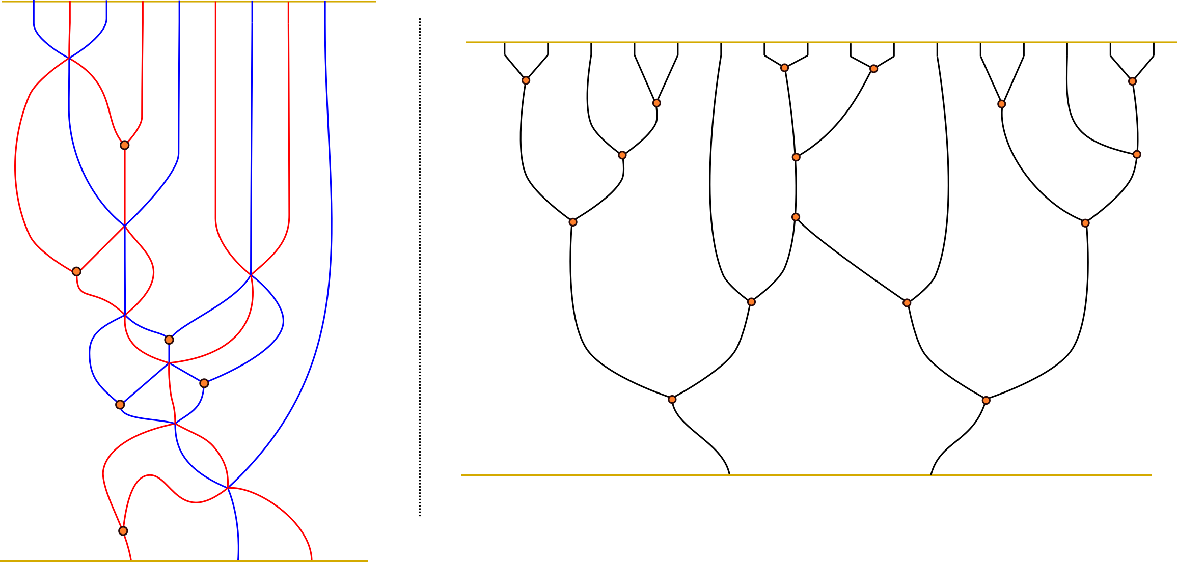
Let $\beta_{1},\beta_{2}$ be two positive $n$ -braid words. By definition, a weave $\mathfrak{w}$ of degree $n$ from $\beta_{2}$ to $\beta_{1}$ , denoted $\mathfrak{w}:\beta_{2}\to\beta_{1}$ , is the image of a continuous map

\mathfrak{w}:\bigcup_{i=1}^{n-1}G_{i}\longrightarrow\mathbb{R}\times[1,2],

where each $G_{i}$ , $i\in[1,n-1]$ is a trivalent graph and the following conditions are satisfied:

(i)

The restriction $\mathfrak{w}|_{G_{i}}:G_{i}\longrightarrow\mathbb{R}\times[1,2]$ is a topological embedding for all $i\in[1,n-1]$ , which is a smooth embedding away from the trivalent vertices of the graph $G_{i}$ .
(ii)

The images $\mathfrak{w}(G_{i})$ and $\mathfrak{w}(G_{i+1})$ are only allowed to intersect at trivalent vertices, $i\in[1,n-2]$ , and the planar edges around this intersection point must alternatingly belong to $G_{i}$ and $G_{i+1}$ . In addition, for $|i-j|\geq 2$ the intersections between $\mathfrak{w}(G_{i})$ and $\mathfrak{w}(G_{j})$ are transverse, and these are not allowed to intersect at trivalent vertices.
(iii)

In a neighborhood of $\mathbb{R}\times\{j\}\subseteq\mathbb{R}\times[1,2]$ , $j=1,2$ , the image $im(\mathfrak{w})$ is given by $l(\beta_{j})$ vertical lines, such that the $k$ th line belongs to $G_{\sigma^{(j)}_{i_{k}}}$ , where $\sigma^{(j)}_{i_{k}}$ is the $k$ th crossing of $\beta_{j}$ .

See Figure 5 for two explicit examples with $n=2,3$ . The image $im(\mathfrak{w})$ of a weave $\mathfrak{w}$ is often referred to as a weave itself and denoted $\mathfrak{w}$ , to ease notation. The intersection of a weave $\mathfrak{w}$ with a small neighborhood of $\mathbb{R}\times\{2\}$ , resp. of $\mathbb{R}\times\{1\}$ , is said to be the top of the weave, resp. its bottom.

Following [25, Section 4], we also introduce a notion of weave equivalence, represented by the local moves in Figure 6. That is, by definition, two weaves $\mathfrak{w}_{1},\mathfrak{w}_{2}$ are said to be (weave) equivalent if they differ by a sequence consisting of moves from Figure 6. See also [24, Section 3.1] and [19, Section 4.2].

Figure 6. Weave equivalences, after [25, Theorem 1.1].

By definition, there is also an additional move called a weave mutation, after [25, Section 4.8], which is not considered as an equivalence. Weave mutation is depicted in Figure 7.

$\longleftrightarrow$

Figure 7. Weave mutation, after [25, Theorem 4.21]. This is not an equivalence.

The definition of weaves and weave equivalence in [25] are manifestly rotationally symmetric. In this paper we would like to break this symmetry by choosing a generic vertical direction and reading a weave top to bottom, allowing only certain local models to appear in such scanning. Similarly to Definition 4.1.(iii) above, a generic horizontal cross-section at the $j$ th level of this type of weave is then a sequence of colored points in $\mathfrak{w}$ which we interpret as a braid word

\beta_{j}(\mathfrak{w})=s^{(j)}_{i_{1}}s^{(j)}_{i_{2}}\cdots s^{(j)}_{i_{\ell(\beta_{j})}}\in\mathrm{Br}_{n}^{+}.

This particular type of weave $\mathfrak{w}$ can then be understood as a “movie” of different braid words:

\mathfrak{w}:=(\beta_{0}(\mathfrak{w})\to\beta_{1}(\mathfrak{w})\to\cdots\to\beta_{\ell(\mathfrak{w})}(\mathfrak{w})).

The initial braid word $\beta_{0}(\mathfrak{w})$ being read at the (top) horizontal cross-section $\mathbb{R}\times\{2\}$ , and the last braid word $\beta_{\ell(\mathfrak{w})}(\mathfrak{w})$ is read at the (bottom) horizontal cross-section $\mathbb{R}\times\{1\}$ . The number $\ell(\mathfrak{w})\in\mathbb{N}$ will be referred to as the length of the weave $\Sigma$ .

Definition 4.2.

Let $\beta_{1},\beta_{2}$ be positive $n$ -braid words. A weave $\mathfrak{w}$ of degree $n$ from $\beta_{2}$ to $\beta_{1}$ is said to be sliced if its cross-sections change top to bottom according to one of the following six situations, depicted in Figure 8:

(a)

Two consecutive edges labeled with the same transposition $s_{k}$ come together, and continue moving down as one unique edge, also labeled with $s_{k}$ , $k\in[1,n-1]$ . This is referred to as a trivalent vertex, and correspond to the model around (the image of) a trivalent vertex of the graph $G_{k}$ in Definition 4.1. Algebraically, we represent this local model by $s_{k}s_{k}\to s_{k}$ .
(b)

Three consecutive edges labeled by $s_{k},s_{k+1},s_{k}$ come together, and continue moving down as three edges but now labeled $s_{k+1},s_{k},s_{k+1}$ . This is referred to as a hexavalent vertex, and correspond to the model around an intersection point of the (images of the) graphs $\mathfrak{w}(G_{k})\cap\mathfrak{w}(G_{k+1})$ in Definition 4.1. Algebraically, we represent this local model by $s_{k}s_{k+1}s_{k}\to s_{k+1}s_{k}s_{k+1}$ . In addition, we also allow the same move, but reversed: $s_{k+1}s_{k}s_{k+1}\to s_{k}s_{k+1}s_{k}$ , with $s_{k+1}s_{k}s_{k+1}$ on top and $s_{k}s_{k+1}s_{k}$ at the bottom.
(c)

Two consecutive edges labeled with two different transpositions $s_{k},s_{j}$ , with $|j-k|\geq 2$ , come together, and continue moving down as two edges, now labeled by $s_{j},s_{k}$ . This is referred to as a 4-valent vertex, and correspond to the model around a (transverse) intersection point of $\mathfrak{w}(G_{k})$ and $\mathfrak{w}(G_{j})$ in Definition 4.1. Algebraically, we represent this local model by $s_{k}s_{j}\to s_{j}s_{k}$ .
(d)

Two consecutive edges labeled with the same transposition $s_{k}$ come together, merge and there is no edge continuing down. This is referred to as a cup, and we represent this local model by $s_{k}s_{k}\to 1$ .
(e)

The inverse of the move in (d), where two consecutive edges are created as moving downwards from the empty set. This is referred to as a cap, and we represent this local model by $1\to s_{k}s_{k}$ .
(f)

There is an edge labeled by $s_{k}$ and it continues moving down as the same edge labeled by $s_{k}$ , i.e. nothing occurs. This local model is represented algebraically by $s_{k}\to s_{k}$ .

By definition, we require that all 3-,4- and 6-vertices, cups and caps appear at different heights, and all horizontal tangencies are isolated. Note that 4-valent and hexavalent vertices represent (the Coxeter projection of the) braid relations. Finally, the following two are special types of sliced weaves that we use:

(ii)

By definition, a simplifying weave is a sliced weave with no caps; thus the only allowed local models are (a),(b),(c),(d) and (f), not (e).
(ii)

By definition, a Demazure weave is a sliced weave with no cups nor caps; thus the only allowed local models are (a),(b),(c) and (f), not (d),(e).

Note that a sliced weave is simplifying if and only if the length of a braid word is not increasing as we scan down the weave with horizontal cross-sections. The reasons behind the choice of the name Demazure weaves will be explained in Section 4.4. Demazure weaves prominently feature in [19]. In this article, all weaves we discuss are sliced and thus from now onwards weave will refer to sliced weave unless otherwise indicated.

Remark 4.3.

A cautious reader might have noticed that some local weave pictures are allowed by the general setup of [25] but do not directly appear in our list (a)-(f) in Figure 8. The upside-down trivalent vertices, i.e. the horizontal flip of model (a), given by $s_{k}\to s_{k}s_{k}$ , can be constructed using the above trivalent vertices and caps, see Section 4.3.2. Similarly, one may encounter a 6-valent vertex with $a$ incoming and $(6-a)$ outgoing edges for any $0\leq a\leq 6$ . All these can be modeled using the usual 6-valent vertices, cups and caps, possibly in several different ways. We declare all such weaves (fixing $a$ and the coloring of edges at the top) equivalent. The same applies to “non-standard” 4-valent vertices, see sections 4.3.4 and 4.3.3 below for details.

Remark 4.4.

For context with [25, Section 7.1.2], we note that Demazure weaves $\mathfrak{w}:\beta_{2}\to\beta_{1}$ are free, in that their fronts can be realized by embedded exact Lagrangian cobordisms from the Legendrian associated to $\beta_{1}$ to the Legendrian associated to $\beta_{2}$ . Indeed, this is implied by the fact that the three models $(a),(b),(c)$ above are decomposable Lagrangian cobordisms. For $(b),(c)$ this follows from the fact that they are traces of Legendrian isotopies, e.g. $(b)$ is the Lagrangian trace of the Legendrian Reidemeister III move. For $(a)$ , this follows from the generic Legendrian perturbation of the $D_{4}^{-}$ front, as drawn in [25, Figure 36], or by comparison to the pinching saddle cobordism, as established in [62, Prop. 3.1]. In particular, a Demazure weave $\mathfrak{w}:\beta\to\Delta$ yields a unique embedded exact Lagrangian filling of the Legendrian associated to $\beta\Delta$ , as the Legendrian unlink, associated to $\Delta^{2}$ , admits a unique embedded exact Lagrangian filling.

4.2. Equivalence of Demazure weaves

Let us now introduce a series of situations, all representing an equivalence between two weaves $\mathfrak{w}_{1},\mathfrak{w}_{2}$ whose top and bottom ends coincide, i.e. $\beta_{0}(\mathfrak{w}_{1})=\beta_{0}(\mathfrak{w}_{2})$ and $\beta_{\ell(\mathfrak{w}_{1})}(\mathfrak{w}_{1})=\beta_{\ell(\mathfrak{w}_{2})}(\mathfrak{w}_{2})$ . The majority of equivalences we describe compare two local models, and an equivalence between two different weaves $\mathfrak{w}_{1},\mathfrak{w}_{2}$ will be obtained by applying several of the local equivalences listed here. We focus on Demazure weaves and their equivalences which only pass through Demazure weaves. In this section we translate the moves of Figure 6 to our formalism.

Remark 4.5.

A cautious reader may choose to call the equivalence relation in this section Demazure equivalence. In principle, it might be possible that two Demazure weaves are not equivalent through Demazure weaves, but are equivalent through the more general weave equivalences from Figure 6. We have not investigated this problem. This fine point is irrelevant for the results of this paper, and we use the same notion of equivalence to simplify the exposition.

Remark 4.6.

In what follows, we also require that the horizontal reflection of each of the upcoming relations explained in 4.2.1–4.2.6 below is also a relation.

4.2.1. Changing the height of vertices.

We allow to change relative heights of any pair of crossings in a weave provided that they are not connected by an edge and there are no crossings between them. (This is commonly called the interchange law in the context of 2-categories.)

4.2.2. Canceling pairs of 4- and 6-valent vertices

The following weaves are declared to be equivalent:

This corresponds to moves (I) and (V) from Figure 6. From the algebraic perspective, i.e. studying the braids in the horizontal cross-sections, this is the diagrammatic incarnation of the fact that the two moves $s_{k}s_{k+1}s_{k}\to s_{k+1}s_{k}s_{k+1}$ and $s_{k+1}s_{k}s_{k+1}\to s_{k}s_{k+1}s_{k}$ , and the two moves $s_{i}s_{j}\to s_{j}s_{i}$ and $s_{j}s_{i}\to s_{i}s_{j}$ , $|i-j|\geq 2$ , are inverse to each other. That is, performing a Reidemeister III move and then its inverse is considered to be (equivalent to) the trivial weave. Similarly, performing a commutation move in the braid group, and then the same move in reverse, is also considered to be (equivalent to) the trivial weave. In the notation above, we are declaring the weave $\mathfrak{w}_{1}=s_{k+1}s_{k}s_{k+1}\to s_{k}s_{k+1}s_{k}\to s_{k+1}s_{k}s_{k+1}$ to be equivalent to the constant weave $\mathfrak{w}_{2}=s_{k+1}s_{k}s_{k+1}$ , and the weave $\mathfrak{w}_{1}=s_{i}s_{j}\to s_{j}s_{i}\to s_{i}s_{j}$ to be equivalent to the constant weave $\mathfrak{w}_{2}=s_{i}s_{j}$ .

4.2.3. Commutation with distant colors

We declare that an edge of the weave labeled with a color (i.e. a transposition) which is distant to the rest of the colors at a given vertex can be moved past this vertex. That is, we declare that the following weaves are equivalent:

Similarly, we declare that three lines with pairwise distant colors can be rearranged according to the weave equivalence depicted above. As illustrated in the equivalences above, the particular sequences of braid moves that we are declaring to be equivalent are read from taking horizontal cross-sections in the above diagrams; we will thus not necessarily indicate them any longer.

4.2.4. 1212- and 2121-relations

We require that the following two ways of getting from $\sigma_{1}\sigma_{2}\sigma_{1}\sigma_{2}$ , denoted 1212 for simplicity, to $\sigma_{1}\sigma_{2}\sigma_{1}$ , i.e. 121, are equivalent:

This corresponds to the move (II) from Figure 6.

We also impose equivalences for other interpretations of the move (II) from Figure 6 using Demazure weaves, corresponding to other paths around the pentagon on the left of the above figure. Namely, we require that the two ways of getting from 1121 to 212 are equivalent, and that the two ways of getting from 2122 to 121 are equivalent, and so forth. The equivalence of the two ways of getting from 1121 to 212 corresponds to the equivalence of the following two simplifying weaves:

We also require that the two ways of getting from 1211 to 212 are equivalent, which is the same as requiring that the two ways of getting from 2121 to 212 are equivalent and so on. The weaves are obtained from the ones above by the symmetry along the vertical line:

There are also similar relations where adjacent colors are interchanged (e.g. black and red), and for any pair of adjacent colors, which we do not draw here.

4.2.5. Cycles for 12121

As an example for the previous relation, we observe that there are many paths in the Demazure graph from 12121 to 212, related by consecutive application of the 1212-relation:

(A)\ 12121\to 21221\to 2121\to 2212\to 212

(B)\ 12121\to 11211\to 1211\to 2121\to 2112\to 212

(C)\ 12121\to 11211\to 1211\to 121\to 212\sim 12121\to 11211\to 1121\to 121\to 212

(D)\ 12121\to 11211\to 1121\to 1212\to 2122\to 212

(E)\ 12121\to 12212\to 1212\to 2122\to 212

Note that the equivalence between (A) and (E) corresponds to the move (III) from Figure 6.

4.2.6. Zamolodchikov relation

Diagrammatically, the Zamolodchikov relation is the equivalence of the following diagrams, relating various braid words for the longest element $w_{0}\in S_{4}$ :

This corresponds to the move (IV) from Figure 6.

4.2.7. Mutations

In contrast with Soergel calculus, we do not declare the two ways of getting from $s_{i}s_{i}s_{i}$ to $s_{i}$ via $s_{i}s_{i}$ to be equivalent. They are related by the following special type of move, which we call a weave mutation:

This concludes the list of diagrammatic equivalences (4.3.5)-(4.2.6), and the mutation non-equivalence (4.2.7).

4.3. Equivalence of simplifying weaves

In this section we define an equivalence relation for simplifying weaves. The complete list of equivalences includes:

(1)

All of the equivalences for Demazure weaves from Section 4.2.
(2)

Changing the relative height of cups and vertices, see Section 4.3.1.
(3)

Additional moves with cups listed in sections 4.3.2(a), 4.3.3(a) and 4.3.4(a).

Remark 4.7.

One can check that the additional equivalence relations for simplifying weaves do not change the total number of cups. Therefore, two Demazure weaves are equivalent through simplifying weaves if and only if they are equivalent through Demazure weaves.

By reflecting these relations along a horizontal axis, we get a similar notion of equivalence for weaves with caps, see 4.3.2(b), 4.3.3(b) and 4.3.4(b). There is an additional “zig-zag” move in section 4.3.5 which allows one to create or delete a cup and a cap simultaneously.

Remark 4.8.

Just as in Remark 4.6, we will require that the horizontal reflection of the relations 4.3.1–4.3.4 are also relations.

4.3.1. Changing the height of vertices II

We allow to change relative heights of any crossing with a cup or cap in a weave, provided that they are not connected by an edge and there are no crossings, cups, or caps between them.

4.3.2. Non-standard trivalent vertices

(a)

We can consider a trivalent vertex with 3 inputs and 0 outputs, defined by either of the pictures:

We require that the two pictures are equivalent, note that both weaves are simplifying.
(b)

We can define an upside-down trivalent vertex in the following ways which are required to be equivalent:

Since both weaves include a cap, these are not simplifying, and we do not allow upside-down trivalent vertices in simplifying weaves.

A horizontal reflection of these relations would express a ”standard” trivalent vertex using an upside-down trivalent vertex and a cup. There is a similar picture to 4.3.2(a) with 0 inputs and 3 outputs.

4.3.3. Non-standard 6-valent vertices

The following relations correspond to different ways to a look at a single 6-valent vertex. We require that all of them are equivalent, provided that the numbers of inputs and outputs are fixed.

(a)

We illustrate simplifying weaves with 4 inputs and 2 outputs, and 5 inputs and 1 output, defined using standard 6-valent vertex and cups. The former in fact implies the latter.

Finally, we can define a 6-valent vertex with 6 inputs and 0 outputs, and the following diagram shows that all ways to do so are equivalent:
(b)

The symmetric pictures with 2 inputs and 4 outputs, 1 input and 5 outputs, and 0 inputs and 6 outputs, are obtained by reflection in the horizontal axis and using caps. These are not simplifying.

4.3.4. Non-standard 4-valent vertices

(a)

Similarly, we can define non-standard 4-valent vertices by simplifying weaves with 3 inputs and 1 output, or 4 inputs and 0 outputs.
(b)

By reflecting these, we get weaves with 1 input and 3 outputs (or 0 inputs and 4 outputs) which use caps. These are not simplifying.

4.3.5. Planar isotopies

A weave in the plane is, in particular, a planar diagram. We declare planar isotopic diagrams to define equivalent weaves. In particular, we need to require the following zigzag relation with canceling pairs of caps and cups:

Algebraically, the weave $\mathfrak{w}_{1}=s_{k}\to s_{k}s_{k}s_{k}\to s_{k}\cdot 1=s_{k}$ , where first a cap creates $1\to(s_{k}s_{k})$ to the left of the initial $s_{k}$ , and then a cup erases the rightmost to $s_{k}$ via $(s_{k}s_{k})\to 1$ , is equivalent to the constant weave $\mathfrak{w}_{2}=s_{k}$ .

Proposition 4.9.

Assume the zigzag relation and the equivalence relations 4.3.2-4.3.4. Then any two planar isotopic weaves are equivalent.

Proof.

By [37, Proposition 3.2] it is sufficient to prove that every vertex is cyclic, that is, invariant under the 360 degree rotation. For a trivalent vertex, we use the definition of the upside down trivalent vertex and relations 4.3.2 to show that a 60 degree rotation changes either of the trivalent vertices to another one of the same type, e.g.:

This implies that a trivalent vertex is invariant under 120 degrees rotation, and hence invariant under 360 degree rotation. Similarly, we can use the relations 4.3.3 to show that the 6-valent vertex is invariant under rotation by 60 degrees, and hence by 360 degrees:

The proof for a 4-valent vertex is similar. We refer to [37, Section 3] and references therein for more details on cyclicity and isotopy invariance. ∎

4.3.6. Rotational invariance

We expect that, similarly to the proof of Proposition 4.9 and the results of [37], the equivalence relations above are rotationally invariant. That is, any rotation of an equivalence relation follows from the relations. We do not need and do not prove it here, but give a couple of examples which illustrate this point:

Note that these two pictures, as planar graphs, are similar to the ones that we already considered (cancellation $121\to 212\to 121$ and $1212$ -move), but in this case they are drawn differently.

Both of these are actually consequences of the above relations. The former follows from the equivalence 4.3.3. For the latter, we can consider the diagram:

All cycles in this diagram are covered by the above relations.

4.4. Demazure product and Demazure weaves

We will use the notion of Demazure product of a word (equivalently, of an expression) in the alphabet of simple reflections $\left\{s_{i}\right\}$ . This terminology is introduced in [73], but the notion goes back at least to [31]. We refer the reader to [29, Section 2.2] for a detailed discussion on this notion and its relation to 0-Hecke algebras over $\mathbb{F}_{2}$ .

The Demazure product of a word $Q=s_{i_{1}}s_{i_{1}}\ldots s_{i_{l}(\beta)}$ , denoted by $\delta(Q)$ , is the largest element of $S_{n}$ in the Bruhat order, such that $Q$ contains some reduced expression of this element as a subword. This element is well-defined. It admits an equivalent inductive definition by the folllowing rule:

\delta(s_{i}):=s_{i},\ \delta(Qs_{i}):=\begin{cases}\delta(Q)s_{i}&\text{if}\ \ell(\delta(Q)s_{i})=\ell(\delta(Q))+1\\ \delta(Q)&\text{if}\ \ell(\delta(Q)s_{i})=\ell(\delta(Q))-1.\\ \end{cases}

It can be verified from either definition that for any $Q,Q^{\prime}$ we have

(4.1)

\begin{split}\delta(Qs_{i}s_{i}Q^{\prime})=\delta(Qs_{i}Q^{\prime});\\ \delta(Qs_{i}s_{i+1}s_{i}Q^{\prime})=\delta(Qs_{i+1}s_{i}s_{i+1}Q^{\prime});\\ \delta(Qs_{i}s_{j}Q^{\prime})=\delta(Qs_{j}s_{i}Q^{\prime}),\,\ |i-j|\geq 2.\end{split}

Given two permutations $u,v\in S_{n}$ , we define their star product $u\star v$ as the Demazure product of the concatenation of an arbitrary reduced expression of $u$ and an arbitrary reduced expression of $v$ . By construction, we have

(u\star v)\star w=\delta(uvw)=u\star(v\star w).

By the Demazure product of an element $\beta$ of the positive braid monoid we mean

\delta(\beta):=\delta(s_{i_{1}}s_{i_{2}}\ldots s_{i_{l}(\beta)})

for a positive braid word $\sigma_{i_{1}}\sigma_{i_{2}}\ldots\sigma_{i_{l}(\beta)}$ for $\beta$ . This is well-defined: by equations (4.1), $\delta(\beta)$ does not depend on the choice of positive braid word.

Example 4.10.

The inductive definition of the Demazure product of a word, and the definition of the star product of permutations imply that

w\star s_{i}=\begin{cases}ws_{i}&\mathrm{if}\;\ell(ws_{i})=\ell(w)+1,\\ w&\mathrm{if}\;\ell(ws_{i})=\ell(w)-1.\end{cases}

Note that the Demazure power of a simple transposition is simply $s_{i}\star s_{i}\star\ldots\star s_{i}=s_{i}$ for any number of multiples. Note also that for any $w\in S_{n}$ we have the equality $w\star w_{0}=w_{0}\star w=w_{0}$ .

In fact, the Demazure product is the product in a monoid known as Coxeter monoid [106], $0-$ Hecke monoid [41, 59], Coxeter $\ast$ -monoid, or Richardson-Springer monoid in the literature. Richardson and Springer studied its action on the set of orbits of the flag variety under the action of the fixed point subgroup of an involution on the algebraic group [94, 95]. Norton [87] constructed a bijection between the set $S_{n}$ and the underlying set of this monoid. As the examples above show, the multiplication in the monoid is quite different from the one in the permutation group. More generally, given a positive braid $\beta$ , $\delta(\beta)$ does not coincide with the image of $\beta$ under the canonical surjection onto $S_{n}$ . A first relation to the weaves introduced above is given in the following lemma.

Lemma 4.11.

Let $\mathfrak{w}$ be a Demazure weave. Then the Demazure product of the associated braid words $\beta_{j}(\mathfrak{w})$ , $j\in[0,l(\mathfrak{w})]$ , remains unchanged, i.e. $\delta(\beta_{0}(\mathfrak{w}))=\delta(\beta_{j}(\mathfrak{w}))$ .

Proof.

Equations (4.1) imply that $3$ -, $6$ - and $4$ -valent vertices preserve the Demazure product. ∎

Lemma 4.11 shows that Demazure weaves provide a transparent diagrammatic interpretation of the Demazure product and of the $0-$ Hecke monoid. This motivated our nomenclature.

4.5. Classification of weaves

We call two weaves equivalent if they are related by a sequence of elementary equivalence moves from Section 4.2 (with no mutations), and mutation equivalent if they are related by a sequence that might involve both equivalence moves and mutations.

Theorem 4.12.

$($ a $)$ Let $\mathfrak{w}_{1},\mathfrak{w}_{2}$ be two weaves such that the source braids of $\mathfrak{w}_{1},\mathfrak{w}_{2}$ coincide and the target braids of $\mathfrak{w}_{1},\mathfrak{w}_{2}$ coincide. If $\mathfrak{w}_{1},\mathfrak{w}_{2}$ only have 6- and 4- valent vertices, then $\mathfrak{w}_{1},\mathfrak{w}_{2}$ are equivalent.

$($ b $)$ Let $\mathfrak{w}_{1},\mathfrak{w}_{2}$ be two Demazure weaves such that the source braids of $\mathfrak{w}_{1},\mathfrak{w}_{2}$ coincide and the target braids of $\mathfrak{w}_{1},\mathfrak{w}_{2}$ coincide. If the target is reduced, then $\mathfrak{w}_{1},\mathfrak{w}_{2}$ are mutation equivalent.

Proof.

The theorem follows from the main result of [36], which we briefly recall. For part (a), consider the graph where vertices correspond to braid words and edges to braid moves (that is, 6- or 4-valent vertices). Then the cycles in this graph are generated by commutation with distant colors and Zamolodchikov relations, hence any two paths in this graph are equivalent.

For (b), consider the Hecke-type algebra with generators $T_{i}$ and relations

T_{i}^{2}=\alpha T_{i}+\beta,\ T_{i}T_{i+1}T_{i}=T_{i+1}T_{i}T_{i+1}+\text{lower order terms},\ T_{i}T_{j}=T_{j}T_{i},(|i-j|>1).

Using these relations, it can be verified that every product of $T_{i}$ can be written as a linear combination of reduced expressions, possibly in a non-unique way. This non-uniqueness appears from ambiguities: applying the relations in different order could yield different results.

B. Elias proved in [36, Proposition 5.5] that (modulo commutation with distant colors) there are exactly 5 types of potential ambiguities that one needs to consider: $iii,ii(i+1)i,i(i+1)ii,i(i+1)i(i+1)i,i(i+1)(i+2)i(i+1)i$ , which are nothing but the trivial move, the 5-cycles corresponding to 1121 and 1211 from 4.2.4, the cycle from 4.2.5 for the word 12121, and the Zamolodchikov relation. Note that the ambiguity $iii$ corresponds to different ways of getting from $iii$ to $i$ . There are two such ways without cups, and they are related by the mutation from Section 4.2.7. ∎

Remark 4.13.

The assumption in (b) that the target is reduced is important. Indeed, the two trivalent vertices $(ss)s\to ss$ and $s(ss)\to ss$ are neither equivalent nor mutation equivalent.

Remark 4.14.

Note that by Theorem 4.12(a), any two simplifying weaves relating two positive braid words for the same braid are equivalent. Thus, we will oftentimes not specify such a weave.

Let us continue studying conditions for equivalences. Suppose that a positive braid word $\beta$ contains a piece $s_{i}us_{j}$ . Following [58], the pair of crossings $(s_{i},s_{j})$ is said to be a deletion pair if $s_{i}u=us_{j}$ . (Note that unlike [58], we do not require $u$ to be a reduced word.) Let us define a relation $\prec$ on the crossings of the braid $\beta$ according to $s_{i}\prec s_{j}$ if $(s_{i},s_{j})$ form a deletion pair. The following two lemmas are used in the proof of the criterion Theorem 4.17 below.

Lemma 4.15.

(i)

The relation $\prec$ is a partial order on the set of crossings of $\beta$ .
(ii)

The set of crossings of $\beta$ is a disjoint union of linearly ordered sets.

Proof.

Assume that we have a piece of a braid $s_{i}us_{j}vs_{k}$ and $(s_{i},s_{j})$ and $(s_{j},s_{k})$ are deletion pairs so that $s_{i}u=us_{j},s_{j}v=vs_{k}$ . Then

s_{i}\cdot us_{j}v=us_{j}s_{j}v=us_{j}v\cdot s_{k},

and $(s_{i},s_{k})$ is a deletion pair. This proves (i). To prove (ii), assume $(s_{i},s_{j})$ and $(s_{i},s_{k})$ are deletion pairs, and assume wlog that $s_{j}$ is to the left of $s_{k}$ . We must show that $(s_{j},s_{k})$ is a deletion pair. We have

s_{i}u=us_{j},\ s_{i}us_{j}v=us_{j}vs_{k},

and $s_{i}us_{j}v=s_{i}uvs_{k}$ . Hence $s_{j}v=vs_{k}$ , and $(s_{j},s_{k})$ is a deletion pair. The case when $(s_{i},s_{k})$ and $(s_{j},s_{k})$ are deletion pairs is analogous. ∎

We call a deletion pair $(s_{i},s_{j})$ close if $s_{i}\prec s_{j}$ is a cover relation, i.e. no crossing in-between $s_{i}$ and $s_{j}$ forms a deletion pair with $s_{i}$ or $s_{j}$ .

Lemma 4.16.

Suppose that $(s_{i},s_{j})$ is a close deletion pair, then the following Demazure weaves are equivalent:

(4.2)

s_{i}us_{j}\to s_{i}s_{i}u\to s_{i}u\to us_{j}\ \sim\ s_{i}us_{j}\to us_{j}s_{j}\to us_{j}.

Note that the condition that the deletion pair is close is necessary, see Remark 4.13.

Proof.

First, note that by Theorem 4.12(a) we can choose a sequence of braid relations relating $s_{i}u$ and $us_{j}$ arbitrarily, and all such weaves would be equivalent. Furthermore, we can choose a braid word for $u$ arbitrarily. Indeed, if $u^{\prime}$ is related to $u$ by braid relations then we get the diagram:

The quadrilaterals on the left and on the right are isotopies, and the rest are built entirely from braid relations and hence are equivalences by Theorem 4.12(a). Therefore the outside pentagon is equivalent to the inside one.

We now prove the statement by induction on the length of $u$ . If $u$ is empty, the statement is clear. Otherwise, by definition of deletion pair we get $s_{i}u=us_{j}$ . If $u$ ends with $s_{j}$ then we do not have a close pair, contradiction. Otherwise we need to apply some braid relation to $us_{j}$ which involves $s_{j}$ . We have the following cases:

1) If $u=vs_{k}$ and $|k-j|>1$ then $us_{j}=vs_{k}s_{j}=vs_{j}s_{k}$ while $s_{i}u=s_{i}vs_{k}$ , so $vs_{j}=s_{i}v$ . We get the following diagram:

The top square is an isotopy, and the pentagon on the right is commutation with distant colors. By the assumption of induction, two Demazure weaves (4.2) corresponding to $s_{i}vs_{j}$ are equivalent, which implies that the bottom pentagon is an equivalence as well.

2) If $u=vs_{j}s_{j+1}$ then $us_{j}=vs_{j}s_{j+1}s_{j}=vs_{j+1}s_{j}s_{j+1}$ while $s_{i}u=s_{i}vs_{j}s_{j+1}$ , so $s_{i}v=vs_{j+1}$ . We get the following diagram:

The top square is an isotopy, and the pentagon on the right is 5-cycle from Section 4.2.4. By the assumption of induction, two Demazure weaves (4.2) corresponding to $s_{i}vs_{j+1}$ are equivalent, and the bottom pentagon is an equivalence as well.

The case when $u=vs_{j}s_{j-1}$ is analogous. ∎

Given a Demazure weave $\mathfrak{w}:\beta_{2}\to\beta_{1}$ , we have an injection $\iota_{\mathfrak{w}}$ from the set of crossings in the bottom $\beta_{1}$ to the set of crossings in the top $\beta_{2}$ . For a 6-valent vertex it is a bijection which exchanges left and right crossings, for a 4-valent vertex it is a bijection exchanging crossings, and for a 3-valent vertex the injection sends the crossing in the target to the right crossing in the source. We refer to the crossings not in the image of $\iota_{\mathfrak{w}}$ as missing. Note that the number of missing crossings equals the number of trivalent vertices and equals $\ell(\beta_{2})-\ell(\beta_{1})$ . The following result is a characterization of the equivalence between Demazure weaves in a special case.

Theorem 4.17.

Let $\beta_{1},\beta_{2}$ be two braid words such that $\ell(\beta_{1})=\ell(\beta_{2})-1$ . Then two Demazure weaves $\mathfrak{w}_{1},\mathfrak{w}_{2}:\beta_{2}\to\beta_{1}$ are equivalent if and only if they have the same missing crossing in $\beta_{2}$ .

Proof.

Since $\ell(\beta_{1})=\ell(\beta_{2})-1$ , any Demazure weave between $\beta_{2}$ and $\beta_{1}$ has one trivalent vertex. Let us prove that equivalent weaves have the same missing crossing. It is verified that commutations with distant colors and Zamolodchikov relations induce the same bijections between crossings, so any two weaves with the same source and target and only 6- and 4-valent vertices induce the same bijection. Finally, for the 5-cycle from Section 4.2.4 we observe that in either weave for 1121 the first crossing is missing, while in either weave for 1211 the third crossing is missing.

Conversely, assume that the Demazure weaves $\mathfrak{w}_{1},\mathfrak{w}_{2}:\beta_{2}\to\beta_{1}$ have the same missing crossing. It is sufficient to prove that they can be related by a sequence of cycles from Lemma 4.16 and equivalences. Note that a trivalent vertex corresponds to a close deletion pair. We have the following cases, where the deletion pair is underlined:

(1)

Assume that $(s_{i},s_{j})$ is a close deletion pair and we apply a 4-valent vertex to $s_{j}$ :

$\underline{s_{i}}u\underline{s_{j}}s_{k}=\underline{s_{i}}us_{k}\underline{s_{j}},\ |k-j|>1,$

then $(s_{i},s_{j})$ is a close deletion pair in the resulting braid, and Lemma 4.16 applies.
(2)

Assume that we apply a 6-valent vertex with $s_{j}$ on the left:

$\underline{s_{i}}u\underline{s_{j}}s_{j+1}s_{j}=\underline{s_{i}}us_{j+1}s_{j}\underline{s_{j+1}}$

then $(s_{i},s_{j+1})$ is a close deletion pair in the resulting braid, and Lemma 4.16 applies.
(3)

Assume that we apply a 6-valent vertex with $s_{j}$ on the right:

$\underline{s_{i}}us_{j}s_{j+1}\underline{s_{j}}=\underline{s_{i}}u\underline{s_{j+1}}s_{j}s_{j+1}$

Note that $s_{i}us_{j}s_{j+1}=us_{j}s_{j+1}s_{j}=us_{j+1}s_{j}s_{j+1}$ implies $s_{i}u=us_{j+1}$ , and $(s_{i},s_{j+1})$ is again a close deletion pair.
(4)

Finally, assume that we apply a 6-valent vertex with $s_{j}$ in the middle, then we no longer get a deletion pair. Instead, $u=vs_{j+1}$ and $s_{i}vs_{j+1}=vs_{j+1}s_{j}$ . By considering possible braid moves, we can write $v=ws_{j}$ , then

$s_{i}ws_{j}s_{j+1}=ws_{j}s_{j+1}s_{j}=ws_{j+1}s_{j}s_{j+1},\$

hence $s_{i}w=ws_{j+1}$ .We get the following diagram:

Here the squares are isotopies and 5-cycle is an equivalence from Section 4.2.4.

By combining all these cases (and the ones obtained by changing $j+1$ to $j-1$ , or applying braid moves to $s_{i}$ ), we can find equivalent weaves $\mathfrak{w}_{1}\sim\mathfrak{w}_{1}^{\prime\prime}\circ\mathfrak{w}_{1}^{\prime}$ and $\mathfrak{w}_{2}\sim\mathfrak{w}_{2}^{\prime\prime}\circ\mathfrak{w}_{2}^{\prime}$ where

•

$\mathfrak{w}_{1}^{\prime},\mathfrak{w}_{2}^{\prime}:\beta_{2}\to\beta^{\prime}$ are weaves between equivalent braid words.
•

$\mathfrak{w}_{1}^{\prime\prime},\mathfrak{w}_{2}^{\prime\prime}:\beta^{\prime}\to\beta_{1}$ are weaves obtained by finding a close deletion pair in $\beta^{\prime}$ and applying either weave from Lemma 4.16, followed by a sequence of braid moves.

Note that $\mathfrak{w}_{1}^{\prime}\sim\mathfrak{w}_{2}^{\prime}$ , so it is enough to check that $\mathfrak{w}_{1}^{\prime\prime}\sim\mathfrak{w}_{2}^{\prime\prime}$ . Since $\mathfrak{w}_{1},\mathfrak{w}_{2}$ have the same missing crossing in $\beta_{2}$ , $\mathfrak{w}_{1}^{\prime\prime}$ and $\mathfrak{w}_{2}^{\prime\prime}$ have the same missing crossing in $\beta^{\prime}$ . Thus, $\mathfrak{w}_{1}^{\prime\prime}$ and $\mathfrak{w}_{2}^{\prime\prime}$ use the same close deletion pair in $\beta^{\prime}$ , so the result now follows from Lemma 4.16. ∎

Remark 4.18.

Although it is natural to consider the above injection and missing crossings for more general weaves, these notions are not invariant under the equivalence relation. Indeed, one can check that the two paths in the 5-cycle for 1121 yield two different injections on crossings (with the same image), and the different paths for 12121 have different missing vertices.

For a positive braid word $\beta$ , we define the mutation graph of $\beta$ to be a graph with vertices given by the equivalence classes of Demazure weaves $\mathfrak{w}:\beta\Delta\to\Delta$ , from $\beta\Delta$ to $\Delta$ , i.e. $\mathfrak{w}\in\mbox{Hom}_{\mathfrak{W}_{n}}(\beta\Delta,\Delta)$ , and edges corresponding to mutations. Note that, by Theorem 4.12(b), any two equivalence classes of Demazure weaves in $\mbox{Hom}_{\mathfrak{W}_{n}}(\beta\Delta,\Delta)$ are related by mutations.

Conjecture 4.19.

Suppose we oriented each mutation in the direction $(ss)s\to s(ss).$ For any positive braid $\beta$ , this orientation descends to the mutation graph of $\beta$ . With this orientation, the mutation graph has no oriented cycles.

The conjecture is motivated by [14], where a similar statement was proven for the exchange graphs for quivers and cluster algebras; see also [15].

4.6. Examples

Let us study two explicit examples in detail, illustrating the material and results presented above.

Example 4.20.

2-strand braids. A braid on two strands is an element of $\mbox{Br}_{2}$ : we denote by $\sigma$ the unique Artin generator of this group, and by $s$ the corresponding Coxeter generator $(12)\in S_{2}$ . Each positive braid $\beta\in\mbox{Br}_{2}$ has a unique braid word, which has the form $\sigma^{l},\,\ l\geq 0$ , and note that $\Delta=\sigma$ . By abuse of notation, we will also write this word as $s^{l}$ . We refer to the braid $\sigma^{l}$ as the $(2,l)$ -torus braid, since its (rainbow) closure is the $(2,l)$ -torus link.

We have no braid moves in $\mbox{Br}_{2},$ so each weave $\mathfrak{w}\in\mathrm{Hom}_{\mathfrak{W}_{2}}(\beta,\beta^{\prime})$ contains only trivalent vertices, cups and caps (and no $6$ - or $4$ -valent vertices). Each Demazure weave $\mathfrak{w}\in\mathrm{Hom}_{\mathfrak{W}_{2}}(\beta\cdot\Delta,\Delta)$ is naturally a rooted binary tree as it contains only trivalent vertices. By construction, all such binary trees with $l(\beta)+1$ leaves are mutualy non-equivalent, but they are all related by mutations. If we orient each mutation $(ss)s\to s(ss),$ the oriented mutation graph will coincide with the classical Hasse graph of the Tamari lattice. It is known to be the $1$ -skeleton of a combinatorial polytope: the $(l(\beta)-1)$ -dimensional associahedron, see e.g. [93]. We can summarize this discussion as follows.

Lemma 4.21.

The mutation graph of the $(2,l)$ torus braid is the $1$ -skeleton of the $(l-1)$ -dimensional associahedron.

We can also understand each Demazure weave $\mathfrak{w}\in\mathrm{Hom}_{\mathfrak{W}_{2}}(s^{l}\cdot\Delta,\Delta)$ as a sequence of openings of crossings in the braid $s^{l}\cdot\Delta=s^{l+1}.$ As we understand trivalent vertices $ss\to s$ as openings of the left crossing, $\mathfrak{w}$ is actually a sequence of openings of crossings in $\beta$ ; the only crossing of $\Delta$ is the crossing of the concave end of $\mathfrak{w}.$ Naturally, the sequence of crossings being opened can be seen as a permutation in $S_{l}.$ The Tamari lattice is known to be both a sublattice and a lattice quotient of the weak order on permutations, see [93]. Note that a permutation is the same as a maximal chain in the Boolean lattice $2^{[l]}$ of the subsets of the set of crossings of $\beta.$

Finally, another way to look at Demazure weaves $\mathfrak{w}\in\mathrm{Hom}_{\mathfrak{W}_{2}}(s^{l}\cdot\Delta,\Delta)$ is to consider them as monotone paths along the edges in the $l-$ dimensional cube, with $2-$ dimensional faces representing elementary moves (equivalences or mutations) between weaves. We illustrate this on the example of the $(2,3)$ -torus braid $\beta=sss$ in Figure 9. Each edge of the cube is oriented downwards and corresponds to one trivalent vertex in a weave. Equivalently, it corresponds to opening a single crossing in $\beta$ . Each vertex represents a horizontal cross-section away from the vertices of a Demazure weave $\mathfrak{w}\in\mathrm{Hom}_{\mathfrak{W}_{2}}(ssss,s)$ ; equivalently, it corresponds to a braid word obtained from $\beta$ by the opening of some crossings. The underlined letters represent crossings that have been opened. For each edge of the weave in a horizontal slice, we can trace back its parents in $ssss$ ; these parents are in parentheses. The cube has the unique top vertex representing the braid $ssss$ , and the unique bottom vertex representing $s$ . Each Demazure weave can be seen as a monotone path along the edges from the top vertex to the bottom vertex.

Figure 9. The Hasse graph of the Boolean lattice

2^{[3]}

. The top vertex is the initial braid word

\beta\cdot\Delta=s^{3}\cdot s=s^{4}

, the bottom vertex represents

\Delta=s

. Demazure weaves

\mathfrak{w}\in\mathrm{Hom}_{\mathfrak{W}_{2}}(ssss,s)

correspond to monotone paths from the top vertex to the bottom vertex.

The yellow face in the cube in Figure 9 illustrates the weave mutation given by

The blue face is the only face that does not represent a mutation. Two monotone paths related by the flip in this face correspond to two different possibilities to draw the same weave in such a way that each horizontal cross-section contains at most one trivalent vertex:

Two weaves are related by a single mutation if they are related by a polygonal flip in a non-blue face. In Figure9, mutations $(ss)s\to s(ss)$ correspond to replacements of two “left” sides of a square by its two “right” sides. The mutation graph is the $1$ -skeleton of $2$ -dimensional associahedron, that is, a pentagon. It is drawn on Figure 10 as the Hasse graph of the Tamari lattice of rooted binary trees with $4$ leaves. This concludes this example, focused on $2$ -stranded braids. The study of $n$ -stranded braids and their weaves is, in general, more intricate (and interesting as well). This is illustrated in the next example.

Figure 10. The mutation graph of the

(2,3)

torus braid

sss

. All mutations are oriented in the direction

(ss)s\to s(ss)

. It coincides with the Hasse graph of the Tamari lattice.

Example 4.22.

The $(3,2)$ torus braid. Consider the $(3,2)$ torus braid $\beta=\sigma_{1}\sigma_{2}\sigma_{1}\sigma_{2}=1212.$ Figure 11 illustrates Demazure weaves $1212\cdot\Delta=1212121\to 212$ and relations between them. In Figure 11, we allow weaves with trivalent vertices $11\to 1,22\to 2$ and $6$ -valent vertices representing braid moves only in one direction: $121\to 212$ . Edges of the graph in Figure 11 represent single moves. We assume that each weave is drawn in such a way that each horizontal cross-section contains at most one vertex. Each vertex on Figure 11 represents a horizontal cross-section without vertices of an (a priori, not unique) weave. All edges are oriented downward. The weaves then correspond to monotone paths from the top vertex to the bottom vertex on the figure.

Figure 11. The top vertex is the initial braid word

\beta\cdot\Delta=s_{1}s_{2}s_{1}s_{2}\cdot s_{1}s_{2}s_{1}

, the bottom vertex represents

s_{2}s_{1}s_{2}

. Demazure weaves

\beta\cdot\Delta\to\Delta

with only

6

-valent vertices

s_{1}s_{2}s_{1}\to s_{2}s_{1}s_{2}

and

3

-valent vertices allowed correspond to monotone paths from the top vertex to the bottom vertex.

It appears that there is a way to draw the graph as a $1-$ skeleton of a $3-$ dimensional polytope with 21 facets, although we did not try to find an explicit polytopal realization. The 2-dimensional (polygonal) faces correspond to the elementary moves between the paths. All the 2-dimensional faces are 4- or 8-gons:

(1)

Yellow quadrilaterals correspond to mutations between the pairs of paths from $sss$ to $s$ .
(2)

Other quadrilaterals correspond to isotopies exchanging the heights of vertices in a weave.
(3)

Octagons correspond to the outer octagons in Section 4.2.5, they are formed by paths (A) and (E). Note that the inner vertices and paths do not appear since the moves $212\to 121$ are not allowed.

We have no words containing $1121$ or $1211$ in our example, so the pentagons from 4.2.4 do not appear. In order to cover all Demazure weaves, we should allow the moves $212\to 121$ . In Figure 11, we should then replace each octagonal face by 5 faces from 4.2.5.

Two weaves are equivalent if the corresponding paths are separated by several white faces, and related by a single mutation if they are separated by one yellow face and several white faces. If we start from some monotone path, replace its part given by some edges of a 2-dimensional face by all the other edges of this face, and repeat this procedure by modifying paths across 2-dimensional faces until we come back to the original path (making the 360 degrees turn around the vertical axis in the polytope along the way), we go by all edges of the mutation graph of equivalence classes of paths exactly once. The mutation graph is a pentagon.

Each Demazure weave $\mathfrak{w}:1212121=\beta\cdot\Delta\to\Delta=121$ is equivalent to a Demazure weave $\mathfrak{w}^{\prime}:\beta\cdot\Delta\to 212$ concatenated with a single $6-$ valent vertex $212\to 121.$ Indeed, if the last vertex in $\mathfrak{w}$ is a $6-$ valent vertex $\beta_{\ell(\mathfrak{w})-1}(\mathfrak{w})=212\to 121=\beta_{\ell(\mathfrak{w})}(\mathfrak{w}),$ then we define $\mathfrak{w}^{\prime}$ to be $\mathfrak{w}$ with this vertex being removed. By construction, $\mathfrak{w}$ is then the concatenation of $\mathfrak{w}^{\prime}$ with this vertex $\beta_{\ell(\mathfrak{w})-1}(\mathfrak{w})\to\beta_{\ell(\mathfrak{w})}(\mathfrak{w}).$ Otherwise, we define $\mathfrak{w}^{\prime}$ to be $\mathfrak{w}$ concatenated with a vertex $121\to 212.$ Then $\mathfrak{w}$ is equivalent to $\mathfrak{w}^{\prime}$ concatenated with a vertex $212\to 121$ via a cancellation move from Section 4.2.2. These arguments show that the mutation graph of Demazure weaves $\beta\cdot\Delta\to\Delta$ is isomorphic to the mutation graph of Demazure weaves $\beta\cdot\Delta\to 212.$ Thus, the former, i.e. the mutation graph of $\beta,$ is also a pentagon.

The appearance of the pentagon is not completely unexpected. Indeed, it coincides with the mutation graph of the torus braid $(2,3)$ .Since the Legendrian links $\Lambda(3,2)=\Lambda(2,3)$ coincide, and the corresponding augmentation varieties are isomorphic. The fact that the mutations graphs of Demazure weaves of these two braids are isomorphic to each other is to be expected.

Let us conclude this subsection on examples with two conjectures. First, inspired by the (Legendrian) equivalence between certain Legendrian $(2,n)$ - and $(n,2)$ -torus links, and Lemma 4.21, we state the following conjecture.

Conjecture 4.23.

For the $(n,2)$ torus braid $\beta$ , the mutation graph of Demazure weaves $\beta\cdot\Delta\to\Delta$ is the $1$ -skeleton of the $(n-1)$ -dimensional associahedron.

Our conjectural 3-dimensional polytope on Figure 11 is similar to polytopes from [81, Figure 1] where the vertices encode equivalence classes of reduced expressions of elements in the braid group and edges correspond to braid moves (also oriented from $s_{i}s_{i+1}s_{i}$ to $s_{i+1}s_{i}s_{i+1}$ ). Reduced expressions are considered to be equivalent if they are related by a sequence of moves $s_{i}s_{j}\to s_{j}s_{i},|i-j|\geq 2$ . This equivalence relation is trivial in our $3-$ strand case. It would be interesting to construct such polytopes for other braids.

Remark 4.24.

The polytopes in [81] are the Hasse graphs of second higher Bruhat orders introduced by Manin and Schechtman [79, 80], see also [107]. Given an arbitrary braid $\beta,$ we can consider a similar oriented graph $D_{\beta}$ . First, we associate a vertex to the braid $\beta$ . We draw edges corresponding to moves $ss\to s,\,s_{i}s_{i+1}s_{i}\to s_{i+1}s_{i}s_{i+1},$ and $s_{i}s_{j}\to s_{j}s_{i},|i-j|\geq 2$ . We then contract all edges corresponding to moves $s_{i}s_{j}\to s_{j}s_{i},|i-j|\geq 2$ . This defines a poset with covering relations defined by edges. An element of the poset is an equivalence class of positive braid words with Demazure product $\Delta$ , with a certain extra decoration. Words are considered to be equivalent if they are related by a sequence of moves $s_{i}s_{j}\to s_{j}s_{i},|i-j|\geq 2$ . The decoration can be understood in terms of subsets of the set of crossings of the braid $\beta$ ; however, it is nontrivial to give a precise definition because of the issue discussed in Remark 4.18. We can also define the decoration in a non-combinatorial way by using variables from Section 5.6.

If we forget the decoration, this poset becomes a poset on the set of words with Demazure product $\Delta$ . Its analogue for all expressions of $\Delta$ and covering relations $ss\to s$ replaced by $ss\to e$ was defined by Elias [36] as an extension of the second higher Bruhat order to necessarily reduced words. It was used in the proof of the main result of the work [36], which we translated to our language as Theorem 4.12. Our weaves thus resemble saturated chains in the second higher Bruhat order, which in turn can be seen as elements of the third higher Bruhat order. However, our equivalence relations differ from the one considered by Manin and Schechtman. Note also that Thomas [105] defined the $0$ th Bruhat order to be the Boolean lattice. As we discussed in Example 4.20, Demazure weaves in $\mathfrak{W}_{2}$ can be seen as maximal chains in the $0$ th Bruhat order. In the present article, we will not explore the link between weaves and the theory of higher Bruhat orders further.

The graph $D_{\beta}$ is not always a $1$ -skeleton of a polytope: e.g. $D_{12122}$ is only a $1$ -skeleton of a union of two quadrilaterals. However, we have the following expectation.

Conjecture 4.25.

For an arbitrary positive braid word $\beta,$ the poset complex of the oriented graph $D_{\beta}$ is either a sphere or a ball. If it is a sphere, it admits a polytopal realization.

4.7. Triangulations and weaves

This subsection provides two types of constructions for weaves, by using certain labeled triangulations, and a relation between them. Specifically, we present the following constructions:

(1)

From an admissible triangulation $\tau$ , as in Definition 4.26 below, we construct a weave $\mathfrak{w}(\tau)$ . There are choices in the construction of $\mathfrak{w}(\tau)$ , but any two sets of choices lead to equivalent weaves.
(2)

From a Demazure triangulation $\underline{\tau}$ , as in Definition 4.30 below, we construct a weave $\mathfrak{w}(\underline{\tau})$ . There are choices in the construction of $\mathfrak{w}(\underline{\tau})$ and, in contrast to (1) above, different choices might lead to non-equivalent weaves. Nevertheless, any two weaves constructed from the same Demazure triangulation $\underline{\tau}$ are mutation equivalent.
(3)

In Proposition 4.39 below we show that any Demazure triangulation can be subdivided to an admissible triangulation, and explain how the resulting weaves – via (1) and (2) above – are related.

In this subsection, weaves are not a priori sliced. The use of the word weave in this subsection will refer to Definition 4.1 unless otherwise specified.

4.7.1. Admissible triangulations and weaves

Given a positive braid word $\beta$ , let us write the letters (crossings) of $\beta\cdot\Delta$ on the sides of a $(\ell(\beta)+\ell(w_{0}))-$ gon.

Definition 4.26.

Let $P\subseteq\mathbb{R}^{2}$ be a regular $n$ -gon. Consider triangulation $\tau$ of $P$ such that the vertices and edges of $P$ are vertices and edges of the triangulation $\tau$ , though $\tau$ may contain vertices inside of $P$ . By definition, $\tau$ is said to be admissible if each of the edges is oriented and labeled by a permutation $u$ such that every triangle is one of the following two types:

That is, either all three sides of one triangle of $\tau$ are labeled by the same simple reflection $s_{i}$ and the edges do not form a 3-cycle, or the sides are labeled by permutations $u,v$ and $u\cdot v$ such that $\ell(u\cdot v)=\ell(u)+\ell(v)$ as depicted above (and edge orientations also are as in the figure). By definition, we call such triangles admissible.

Remark 4.27.

Note that the edges in $\tau$ are oriented, but the triangles are not oriented, and so neither is the triangulation $\tau$ itself. The orientation on edges is used below only to illustrate the way we read and concatenate edge labels: if we follow the edge labeled by $u$ in the direction opposite to its orientation, then we read the label as $u^{-1}$ .

Now, given an admissible triangulation $\tau$ as in Definition 4.26, we can algorithmically construct a weave $\mathfrak{w}(\tau)$ associated to it. For this, we make some additional choices. This is done as follows:

(1)

Choose a reduced expression for the permutation on every edge. For triangles of the second type, we then concatenate the reduced expressions for $u$ and $v$ and get a reduced expression for $uv$ . This can be represented by a (piece of a) weave with no vertices at all. Now, this resulting reduced expression for $uv$ is possibly different from the one initially assigned to $uv$ . Since two reduced expressions are related by a sequence of braid moves, which are translated to 6- and 4-valent vertices for weaves, we can draw a weave (just with 4- and 6-valent vertices) representing that sequence and connecting these two reduced expressions for $uv$ . Note that the resulting weave on such a triangle of the second type depends on this choice of a sequence of braid moves. That said, any two such weaves are related by weave equivalences, by Theorem 4.12.(a).
(2)

For triangles of the first type, with edges labeled by $s_{i}$ , we associate a weave consisting of a single trivalent vertex of the corresponding color $s_{i}$ .

In summary, the possible choices in $(1)$ give equivalent weaves and there are no choices in $(2)$ , for triangles of the first type. Therefore, this assignment of a weave for each triangle in $\tau$ glues up to a weave $\mathfrak{w}(\tau)$ on the entire polygon $P$ , well-defined up to weave equivalence. (Cf. Remark 4.14.)

We can encode some of the moves between weaves in terms of admissible triangulations, as follows:

(i)

Given three permutations $u$ , $v$ and $w$ such that $\ell(uvw)=\ell(u)+\ell(v)+\ell(w)$ , we can make the following moves, which clearly do not change the weave, up to equivalence:

For unlabeled triangulations, these are precisely the Pachner moves (also known as bistellar flips) in dimension $2$ . The result of Pachner [88] states that all triangulations of a polygon are related by such moves (the general version of this result holds for piecewise linear manifolds and bistellar flips in higher dimensions).
(ii)

If we have four permutations $u,v,w,t$ such that $uv=tw$ , then $u^{-1}t=vw^{-1}$ . Assuming that all these products are reduced, we have a move

Note that in this case we get the equations

$\ell(u)+\ell(v)=\ell(t)+\ell(w),\ \ell(u)+\ell(t)=\ell(v)+\ell(w)$

which imply

$\ell(u)=\ell(w),\ \ell(v)=\ell(t).$
(iii)

We can encode the 1212-move from Section 4.2.4 as the following move between triangulations:

Example 4.28.

The weave corresponding to either of the following two diagrams is a 6-valent vertex:

The choice of a reduced expression ( $121$ or $212$ ) on the diagonal determines the triangle containing this 6-valent vertex. This illustrates $(ii)$ above.

Remark 4.29.

Conversely to the construction above, given a weave we can consider the dual planar graph. It has triangular regions corresponding to 3-valent vertices in the weave, hexagonal regions corresponding to 6-valent vertices, and quadrilateral regions corresponding to 4-valent vertices. By choosing any admissible triangulation of each hexagon and quadrilateral, we get a triangulation of the entire polygon. The choice of the triangulation does not matter - for example, for the hexagon with sides labeled 1,2,1,2,1,2 there are 14 triangulations and 12 of them (those that do not contain triangles formed by three diagonals) are admissible. From Example 4.28, any two of them can be related by a sequence of the above moves, and correspond to equivalent weaves. In conclusion, we have a construction starting with a weave and resulting in a triangulation and vice versa. These constructions depend on choices and neither of them is a bijection. For future work, it would be interesting to find a complete set of moves between triangulations such that the corresponding equivalence classes are in bijection with the equivalence classes of weaves.

4.7.2. Demazure triangulations

The correspondence between weaves and admissible triangulations in Subsection 4.7.1 above is clear combinatorially. Nevertheless, it has a disadvantage: given a triangulation, it is unclear if the corresponding weave is simplifying or Demazure (more precisely, it is unclear whether the underlying colored graph can be drawn as a sliced weave which is simplifying or Demazure, respectively) or, geometrically, if the corresponding Lagrangian surface is embedded in $\mathbb{R}^{4}$ (instead of merely immersed). In order to resolve this issue, we now introduce a special class of triangulations – with different labeling rules – which we refer to as Demazure triangulations. We stress that Demazure triangulations are not necessarily admissible triangulations, as defined in Subsection 4.7.1 above. That said, Proposition 4.39 below explains how to produce admissible triangulations from Demazure triangulations by a subdivision process.

Let $\beta$ be a positive $n$ -braid word with Demazure product $\delta(\beta)=w_{0}$ and set $N:=\ell(\beta)+1$ . Consider an $N$ -gon $P$ whose vertices are labeled clockwise with integers from $0$ to $N-1$ . Label the first $N-1$ sides clockwise by the letters of $\beta$ , and label the last (or bottom) side connecting $N-1$ and $0$ by $w_{0}$ . By definition, such labeled polygon $P$ is said to be labeled according to $\beta$ .

Definition 4.30.

Let $\beta$ be a positive $n$ -braid word with Demazure product $\delta(\beta)=w_{0}$ and $P$ a polygon labeled according to $\beta$ . By definition, a Demazure triangulation $\underline{\tau}(P,\beta)$ is a non-oriented triangulation of $P$ with edges labeled by permutations such that:

(1)

The only vertices of $\underline{\tau}(P,\beta)$ are the vertices of $P$ .
(2)

Every edge is labeled by a permutation as follows. An edge $e$ in $\underline{\tau}(P,\beta)$ divides the boundary $\partial P$ into two connected components, and the labels in the connected component of $\partial P$ that does not contain the $w_{0}$ -label spell a subword $\beta^{\prime}\subseteq\beta$ . Then the permutation assigned to $e$ is the Demazure product $\delta(\beta^{\prime})$ of such subword $\beta^{\prime}$ .

Figure 12. (Left) A Demazure triangulation for the braid word

\beta=\sigma_{2}\sigma_{1}^{2}\sigma_{2}^{2}\sigma_{1}^{2}\sigma_{2}\sigma_{1}^{2}\sigma_{2}

. The Demazure product

w_{0}=s_{1}s_{2}s_{1}

and its associated edge are depicted in green for visual emphasis. (Right) A possible weave associated to this Demazure triangulation.

First, a Demazure triangulation, as in Definition 4.30, is not necessarily admissible, as in Definition 4.26. Note also that the edges of a Demazure triangulation are diagonals of the polygon $P$ and we sometimes refer to them as diagonals. Second, there are no choices in the definition of a Demazure triangulation beyond the triangulation of the polygon $P$ itself and the braid word for $\beta$ . These two uniquely specify the labeling of the edges. Additional choices will be needed when we try to associate a weave to a Demazure triangulation. By definition, any Demazure triangulation of a polygon labeled according to $\beta$ is said to be a Demazure triangulation of $\beta$ , and we often simply write $\underline{\tau}(\beta)$ for such a Demazure triangulation.

Example 4.31.

Figure 12 (left) illustrates an instance of a Demazure triangulation. The positive 3-braid word is $\beta=\sigma_{2}\sigma_{1}^{2}\sigma_{2}^{2}\sigma_{1}^{2}\sigma_{2}\sigma_{1}^{2}\sigma_{2}$ , whose Demazure product is indeed $w_{0}=s_{1}s_{2}s_{1}$ .

Definition 4.32.

Given a Demazure triangulation, we define the height of the bottom $w_{0}$ -side to be 0. Given any other side or edge, we define its height as the number of edges separating it from the bottom side plus one.

Example 4.33.

The following picture illustrates edges in a triangulation labeled by height, where the bottom side is labeled with $w_{0}$ :

By definition, in any triangle in a Demazure triangulation we have two sides of equal height $h$ labeled by some permutations $u,v$ and the third side of height $h-1$ labeled by $u\star v$ .

Definition 4.34.

Let $\triangle$ be a triangle with sides $u,v$ and $u\star v$ . The defect of $\triangle$ is

\dft(\triangle)=\ell(u)+\ell(v)-\ell(u\star v).

The following fact relates defects to the length of the boundary braid.

Lemma 4.35.

Let $\beta$ be a positive braid word and $\triangle$ a triangle in a Demazure triangulation of $\beta$ . Then

\sum_{\triangle}\dft(\triangle)=\ell(\beta).

Proof.

Set $r:=\ell(\beta)$ to ease notation and let us prove the following more general statement: “Suppose that a diagonal, or the side with vertices $0$ and $N$ , encloses a braid $\beta^{\prime}$ with $k$ crossings, and carries the label $u=\delta(\beta^{\prime})$ . Then the sum of defects of the triangles above this diagonal equals $k-\ell(u)$ .” The required statement in the lemma follows from this by setting $u=w_{0}$ , so that we have $r+\ell(w_{0})-\ell(w_{0})=r$ .

To prove this general statement, we use induction in $k\in\mathbb{N}$ . Consider the triangle adjacent to the diagonal with $u$ , its other sides are labeled $v$ and $w$ such that $v\star w=u$ . By the assumption of induction, sum of defects above $v$ equals $k_{1}-\ell(v)$ and the sum of defects above $w$ equals $k_{2}-\ell(w)$ , with $k_{1}+k_{2}=k$ , so the total sum of defects equals $k_{1}-\ell(v)+k_{2}-\ell(w)+\ell(v)+\ell(w)-\ell(u)=k-\ell(u).$ ∎

The next result justifies the chosen nomenclature for a Demazure triangulation.

Proposition 4.36.

Let $\beta$ be a positive braid word with Demazure product $\delta(\beta)=w_{0}$ , $\Delta$ a reduced word for $w_{0}$ , and $\underline{\tau}(\beta)$ a Demazure triangulation associated to $\beta$ . Then there exists a non-deterministic algorithm that constructs a Demazure weave $\mathfrak{w}(\underline{\tau}(\beta))\in\mathrm{Hom}_{\mathfrak{W}_{n}}(\beta,\Delta)$ from the Demazure triangulation $\underline{\tau}(\beta)$ .

Before its proof, we emphasize that there are choices in the construction of a Demazure weave $\mathfrak{w}(\underline{\tau}(\beta))$ from the Demazure triangulation $\underline{\tau}(\beta)$ . Different choices for the same $\underline{\tau}(\beta)$ lead to mutation-equivalent, but not necessarily weave-equivalent, weaves.

Proof.

First, observe that for any two permutations $u,v$ there exists a (non-unique) Demazure weave from the concatenation of any reduced braid words for $u$ and $v$ at the top to any reduced word for $u\star v$ at the bottom. This is immediate by the definition of Demazure product: we can go from $uv$ to $u\star v$ by a sequence of braid relations and moves $s_{i}s_{i}\to s_{i}$ , which correspond to 6-,4- and 3-valent vertices. Therefore, for each triangle of the Demazure triangulation, we have a Demazure weave from the concatenation of the reduced words for the labels of the sides of height $h$ to the reduced word for the label of the height $h-1$ . Note that such Demazure weaves associated to a triangle might not be unique, but at least one exists. Given a Demazure triangulation, we now construct a Demazure weave as follows.

For each possible height $h$ there is a unique polygonal chain $L_{h}$ inside the Demazure triangulation, consisting of diagonals of the triangulation of height $h$ and (some) sides of the polygon of height at most $h$ , and satisfying the following conditions:

(i)

Its two endpoints coincide with the endpoints of the bottom side.
(ii)

It contains all diagonals of height $h$ precisely once, and each side of the polygon at most once.

For each diagonal or side appearing in $L_{h}$ , we choose a reduced expression of its label; for the bottom side, we choose $\Delta$ as a reduced word for $w_{0}$ , and for each other side its label is a letter of $\beta$ . The clockwise orientation of the boundary of the polygon induces an orientation on the bottom side. We define $\beta_{h}$ to be the concatenation of all the words appearing as labels of the line segments appearing in $L_{h}$ , where we orient $L_{h}$ from the target of the oriented bottom side to its source. Note that we have $\beta_{0}=\Delta$ and $\beta_{N-3}=\beta$ . By the discussion above, for each height $h$ , there exists a (non-unique) Demazure weave from $\beta_{h}$ to $\beta_{h-1}$ . By choosing such a weave for each height $h$ and concatenating them we obtain a Demazure weave from $\beta$ to $w_{0}$ . ∎

Figure 13. (Left) A weave mutation. (Right) A move obtained from composing a sequence of weave equivalences, one weave mutation and another sequence of weave equivalences.

Remark 4.37.

As stated in the proof above, note that there are several ways to fill a triangle of a Demazure triangulation with a (piece of a) weave. For instance, if all sides are labeled with the same permutation $121$ , we have the two options in Figure 13 (right), which are mutation equivalent but not weave-equivalent. In Figure 14 we depict (some) possible pieces of weaves that can appear in triangles of a Demazure triangulation with only 2 colors, i.e. for permutations in $s_{1},s_{2}\in S_{3}$ .

4.7.3. Relation between Demazure triangulations and admissible triangulations

Demazure triangulations, discussed in Subsection 4.7.2, relate to admissible triangulations, discussed in 4.7.1, as follows.

To ease notation, we say that a weave is compatible with a Demazure triangulation $\underline{\tau}$ if it can be obtained from $\underline{\tau}$ using the construction in the proof of Proposition 4.36. Note that there are typically different (non-equivalent) weaves compatible with the same Demazure triangulation $\underline{\tau}$ , cf. Remark 4.37. Similarly, a weave is said to compatible with an admissible triangulation $\tau$ if it can be obtained from $\tau$ using the construction in Subsection 4.7.1. In this case, any two weaves compatible with the same admissible triangulation $\tau$ are weave equivalent.

Let $\beta$ a positive braid word with Demazure product $w_{0}$ and fix a reduced expression $\Delta$ for $w_{0}$ as in Proposition 4.36. Consider a Demazure triangulation $\underline{\tau}$ of $\beta$ . This is a triangulation $\underline{\tau}$ of a polygon with $l(\beta)+1$ sides, where the summand $1$ accounts for the edge that is labeled with $w_{0}$ . In order to relate it to an admissible triangulation for $\beta$ , which triangulates a polygon with $l(\beta)+l(w_{0})$ sides, we need to account for this difference in the number of sides. This is achieved as follows:

Definition 4.38.

Let $\underline{\tau}(\beta)$ be Demazure triangulation of $\beta$ , $\Delta$ a reduced expression for $w_{0}$ and $\underline{\tau}(\Delta^{op})$ a Demazure triangulation for $\Delta^{op}$ . By definition, a $\Delta$ -expansion of $\underline{\tau}(\beta)$ is the triangulation of a polygon with $l(\beta)+l(w_{0})$ sides obtained by gluing $\underline{\tau}(\beta)$ and $\underline{\tau}(\Delta^{op})$ along their (correspondingly unique) $w_{0}$ -edges. By definition, a $w_{0}$ -expansion is a $\Delta$ -expansion, for some (unspecified) reduced expression $\Delta$ of $w_{0}$ .

We refer to any such triangulation, as in Definition 4.38 for some choice of reduced expression for $\Delta$ , as a $w_{0}$ -expansion of $\underline{\tau}(\beta)$ .

Proposition 4.39.

Let $\beta$ be a positive braid word. Any $w_{0}$ -expansion of a Demazure triangulation $\underline{\tau}(\beta)$ for $\beta$ can be subdivided and oriented to obtain an admissible triangulation $\tau(\beta)$ for $\beta$ . In addition, any weave compatible with $\tau(\beta)$ is compatible with $\underline{\tau}(\beta)$ .

Proof.

Consider a triangle in a Demazure triangulation with sides $u,v$ and $u\star v=\delta(uv)$ . If $u\star v=uv$ , then this triangle is admissible. Otherwise, we use induction in $\ell(v)$ . Let $v_{1}$ be the longest prefix of $v$ such that $uv_{1}$ is reduced. Then we can write $v=v_{1}sv_{2}$ such that $\ell(uv_{1})=\ell(u)+\ell(v_{1})$ but $\ell(uv_{1}s)<\ell(u)+\ell(v_{1})+1$ . Therefore we can find a reduced expression $w$ such that $uv_{1}=ws$ , and draw the following diagram:

The unmarked edges are labeled by $ws=uv_{1},ws$ and $sv_{2}$ . Now

u\star v=u\star v_{1}\star s\star v_{2}=w\star s\star s\star v_{2}=ws\star v_{2},

and by the assumption of induction we can subdivide the marked triangle with sides $ws$ and $v_{2}$ into admissible ones. In this manner, we subdivide each triangle in an arbitrary Demazure triangulation into admissible triangles. Therefore, we can subdivide each $w_{0}$ -expansion of $\underline{\tau}(\beta)$ (recall that it is glued out of two Demazure triangulations) into a triangulation consisting of admissible triangles, which is then admissible by definition. Let us denote this admissible triangulation by $\tau(\beta)$ .

For the statement about the weave, let us describe an arbitrary weave compatible with $\tau(\beta)$ as a sequence of braid words. First, given a subdivided triangle as above, we choose some word for $u,v_{1},v_{2}$ and use a sequence of braid relations

uv\to uv_{1}sv_{2}\to wssv_{2}

Next, we insert a trivalent vertex in the central triangle and get $wsv_{2}$ , and proceed by induction. This yields one possible sequence of moves computing the Demazure product $u\star v$ . This gives a Demazure weave for each triangle in $\underline{\tau}(\beta)$ . Gluing them together, we get a Demazure weave $\mathfrak{w}_{1}$ compatible with $\underline{\tau}(\beta)$ , as in the proof of Proposition 4.36. Doing the same for each triangle in our chosen Demazure triangulation for $\Delta^{op}$ , where we fixed the word $\Delta^{op}$ on the bottom side, we obtain a Demazure weave $\mathfrak{w}_{2}$ from $\Delta^{op}$ to itself. Now we can glue these two weaves $\mathfrak{w}_{1},\mathfrak{w}_{2}$ together along their $w_{0}$ -edges and declare that all the consecutive edges that spell $\Delta^{op}$ , i.e. all the edges from $\mathfrak{w}_{2}$ except its $w_{0}$ -edge, are to be considered as one edge (indeed, since the polygons for $\beta$ and for $\Delta^{op}$ have opposite orientations, the gluing can in fact be interpreted as the concatenation of $\mathfrak{w}_{1}$ with the half-turn of $\mathfrak{w}_{2}$ , the latter being a Demazure weave from $\Delta$ to itself). By labeling this particular edge with $w_{0}$ , the result of gluing $\mathfrak{w}_{1}$ and $\mathfrak{w}_{2}$ and performing this identification gives a weave compatible with $\underline{\tau}(\beta)$ . Indeed, it is compatible with $\underline{\tau}(\beta)$ because $\mathfrak{w}_{2}$ consists only of 4- and 6-valent vertices. In fact, this resulting weave is equivalent to $\mathfrak{w}_{1}$ by Theorem 4.12.(a). ∎

5. Algebraic Weaves, Morphisms, and Correspondences

This section develops the relative geometry of braid varieties, studying morphisms and correspondences between them. These correspondences are defined using weaves, and provide a functor from the category of algebraic weaves to the category of algebraic varieties and their correspondences. Here and below, a correspondence between $X$ and $Y$ is an algebraic variety $Z$ with two regular maps $Z\to X$ and $Z\to Y$ . In general, we do not require that $Z$ is a subset of $X\times Y$ . That said, this stronger condition does hold for correspondences associated with simplifying weaves, see Remark 5.10.

5.1. Correspondences

In this section, we use horizontal yellow segments in order to keep track of certain variables, corresponding to the $z_{i}$ -variables in the braid variety. By definition, a horizontal segment inside the domain $\mathbb{R}\times[1,2]$ , where a weave is drawn, is any connected segment contained in a line of the form $\mathbb{R}\times\{r\}$ , for some real value $r\in[1,2]$ . In addition, we also consider particular types of weaves. Altogether, this leads to the following definition.

Definition 5.1.

An algebraic weave of degree $n$ is a sliced weave $\mathfrak{w}\subseteq\mathbb{R}\times[1,2]$ of degree $n$ such that:

(i)

The edges have been oriented downwards, with the models according to Figure 15 for cups and caps. By convention, diagrams are oriented from top to bottom, from $\mathbb{R}\times\{2\}$ down to $\mathbb{R}\times\{1\}$ .
(ii)

The weave $\mathfrak{w}$ is decorated with horizontal yellow rays, as follows. By definition, yellow rays are horizontal rays of the form $(-\infty,b]\times\{r\}\subseteq\mathbb{R}\times[1,2]$ , for some $b\in\mathbb{R}$ and $r\in(1,2)$ , such that the yellow ray starts at a trivalent vertex, or at the bottom of a cup, or at the top of a cap. The first three diagrams in Figure 15, excluding the rightmost picture, depict the three possible starts of a yellow ray. In other words, the starting point $(b,r)\in\mathbb{R}\times[1,2]$ of a yellow ray must either be a trivalent vertex, the lowest point of a cup or the highest point of a cap.
(iii)

The weave $\mathfrak{w}$ is such that any horizontal line $\mathbb{R}\times\{h\}$ , for some $h\in[1,2]$ , contains at most one of the following types of points: a vertex of $\mathfrak{w}$ , the lowest point of a cup or the highest point of a cap.

In particular, all vertices, cups and caps of $\mathfrak{w}$ have different heights, and yellow rays never pass through another vertex, cup or cap (in addition to the starting point), yellow rays are all parallel to each other and are all transverse to the edges of $\mathfrak{w}$ . Therefore, the only local models involving an intersection between a yellow ray and $\mathfrak{w}$ are as depicted in Figure 15.

By definition, a (transverse) intersection point of a yellow ray with a weave edge, distinct from the starting point of the yellow ray, will be referred to as a virtual vertex. A virtual vertex is drawn in the rightmost diagram of Figure 15.

Remark 5.2.

Throughout this section, we refer to the valency of a vertex in the original weave $\mathfrak{w}$ , without accounting for any additional valency due to yellow rays. In particular, trivalent vertices will be still called trivalent despite an additional edge starting at them.

Figure 15. Local models for algebraic weaves, compare with Figure 8. The starting point of a yellow ray must be at a trivalent vertex, a cup or a cap. These cases are respectively labeled with

(a)

(d)

and

(e)

. A virtual vertex is shown on the right.

By Definition 5.1, the new local models for algebraic weaves involving yellow rays are those in Figure 15. The weave edges of the original weave $\mathfrak{w}$ are subdivided by the virtual vertices into smaller segments, and yellow rays are subdivided into intervals, which we often refer to as yellow segments.

Figure 16. The space

\mathbb{V}^{\mathfrak{w}}

for this algebraic weave

\mathfrak{w}

\mathbb{C}^{15}\times\left(\mathbb{C}^{\binom{3}{2}}\times(\mathbb{C}^{\ast})^{3}\right)^{4}

. Indeed, there are 15 weave segments, each labeled with a variable

z_{i}\in\mathbb{C}

, and 4 yellow segments, each labeled with an invertible triangular matrix

U_{j}

. The correspondence

\mathcal{M}(\mathfrak{w})

associated to this algebraic weave is a closed subvariety of

\mathbb{V}^{\mathfrak{w}}

Let $\mathfrak{w}:\beta_{2}\to\beta_{1}$ be an algebraic weave from $\beta_{2}$ , at the top, to $\beta_{1}$ , at the bottom. We now construct a correspondence between the two braid varieties $X_{0}(\beta_{1})$ and $X_{0}(\beta_{2})$ . To each segment of an edge labeled by $i$ we associate a variable $z$ and the braid matrix $B_{i}(z)$ . Segments of a weave edge separated by a virtual vertex carry different variables. In addition, each yellow segment (a segment of a yellow ray) is labeled by an invertible upper triangular matrix whose entries are considered variables as well. All these variables and matrices can be considered as coordinates in the space

\mathbb{V}^{\mathfrak{w}}:=\mathbb{C}^{\mathrm{weave\ segments}}\times\left(\mathbb{C}^{\binom{n}{2}}\times(\mathbb{C}^{\ast})^{n}\right)^{\mathrm{yellow\ segments}},

where we are identifying the space of invertible upper triangular $n\times n$ -matrices with $\mathbb{C}^{\binom{n}{2}}\times(\mathbb{C}^{\ast})^{n}$ . See Figure 16 for an example. The correspondence associated to an algebraic weave $\mathfrak{w}$ is a closed subvariety of $\mathbb{V}^{\mathfrak{w}}$ . This correspondence is defined using the following notion of monodromy.

Definition 5.3.

Let $\mathfrak{w}$ be an algebraic weave and $\tau:[0,1]\to\mathbb{R}\times[1,2]$ a regular parametrization of an oriented embedded path transverse to both $\mathfrak{w}$ and its yellow rays. By definition, the monodromy of the weave $\mathfrak{w}$ along $\tau$ , also referred to as the monodromy of $\tau$ , is the ordered product of the following matrices:

(i)

$B_{i}(z)$ , if the path $\tau$ crosses an edge labeled by $i$ with variable $z$ from left to right,
(ii)

$B_{i}(z)^{-1}$ , if the path $\tau$ crosses an edge labeled by $i$ with variable $z$ from right to left,
(iii)

$U$ , if the path $\tau$ crosses a yellow segment colored by $U$ from top to bottom,
(iv)

$U^{-1}$ , if the path $\tau$ crosses a yellow segment colored by $U$ from bottom to top.

In detail, let $\{t_{1},\ldots,t_{f}\}\in[0,1]$ with $t_{1}<\ldots<t_{f}$ be the times such that $\tau(t_{i})$ intersects either the weave or a yellow ray, and let $M(t_{i})$ be the matrix associated to that intersection point and its intersection sign, according to $(i)$ through $(iv)$ above. Then the monodromy of $\tau$ is the product $M(t_{1})\cdot\ldots\cdot M(t_{f})$ .

Definition 5.4.

Let $\mathfrak{w}$ be an algebraic weave. By definition, the correspondence variety $\mathcal{M}(\mathfrak{w})$ associated to the weave $\mathfrak{w}$ is the affine algebraic subvariety of $\mathbb{V}^{\mathfrak{w}}$ cut out by the following two conditions:

(1)

The monodromy of a closed loop around a neighborhood of every vertex of $\mathfrak{w}$ is the identity.
(2)

The monodromy of a closed loop around a neighborhood of every virtual vertex is the identity.

The two conditions $(1)$ and $(2)$ in Definition 5.4 can be written in terms of polynomial equations on the $z$ -variables and the coefficients of the invertible upper-triangular matrices. Therefore $\mathcal{M}(\mathfrak{w})\subseteq\mathbb{V}^{\mathfrak{w}}$ is a closed affine algebraic subvariety.

5.2. Properties of correspondences

From the ambient space $\mathbb{V}^{\mathfrak{w}}$ associated to $\mathfrak{w}:\beta_{2}\to\beta_{1}$ , we have two natural projections

\mathbb{C}^{\ell(\beta_{1})}\leftarrow\mathbb{V}^{\mathfrak{w}}\rightarrow\mathbb{C}^{\ell(\beta_{2})}.

The projection $\mathbb{V}^{\mathfrak{w}}\rightarrow\mathbb{C}^{\ell(\beta_{2})}$ is given by reading the labels $z_{j}$ associated to the weave segments at the top boundary of $\mathfrak{w}$ , corresponding to crossings of $\beta_{2}$ . Similarly, the projection $\mathbb{V}^{\mathfrak{w}}\rightarrow\mathbb{C}^{\ell(\beta_{1})}$ is given by reading the labels $z_{j}$ associated to the weave segments at the bottom boundary of $\mathfrak{w}$ , which correspond to crossings of $\beta_{1}$ . By considering the braid matrices associated to $\beta_{1}$ and $\beta_{2}$ , we obtain the corresponding maps

\operatorname{GL}(n)\xleftarrow{B_{\beta_{1}}}\mathbb{V}^{\mathfrak{w}}\xrightarrow{B_{\beta_{2}}}\operatorname{GL}(n).

These two maps can be thought of as monodromies along the left to right horizontal paths near the top boundary of $\mathfrak{w}$ , in the case of $B_{\beta_{2}}$ , and near the bottom boundary of $\mathfrak{w}$ , for $B_{\beta_{1}}$ . More generally, if a horizontal slice of $\mathfrak{w}$ spells out a braid word $\beta$ , the corresponding braid matrix defines a map $B_{\beta}:\mathbb{V}^{\mathfrak{w}}\to\operatorname{GL}(n)$ .

Definition 5.5.

Let $\mathfrak{w}:\beta_{2}\to\beta_{1}$ be an algebraic weave of degree $n$ and $\pi\in S_{n}$ a permutation. The closed subvariety $\mathcal{M}(\mathfrak{w},\pi)\subseteq\mathcal{M}(\mathfrak{w})\subseteq\mathbb{V}^{\mathfrak{w}}$ is given by the condition that $B_{\beta_{1}}\pi$ is upper triangular. There exists a natural map $\mathcal{M}(\mathfrak{w},\pi)\to X_{0}(\beta_{1},\pi)$ given by projecting to the labels associated to the bottom boundary segments of $\mathfrak{w}$ , which spell $\beta_{1}$ .

Proposition 5.6.

Let $\mathfrak{w}_{1}:\beta_{1}\to\beta_{0}$ and $\mathfrak{w}_{2}:\beta_{2}\to\beta_{1}$ be algebraic weaves and $\mathfrak{w}:=\mathfrak{w}_{1}\circ\mathfrak{w}_{2}$ their composition. Then the following hold:

(a)

Let $\pi\in S_{n}$ be a permutation, which we represent by a homonymous permutation matrix $\pi\in\operatorname{GL}_{n}(\mathbb{C})$ . Suppose that the matrix $B_{\beta_{1}}\cdot\pi$ is upper-triangular. Then $B_{\beta_{2}}\cdot\pi$ is upper-triangular and $\mathcal{M}(\mathfrak{w}_{2},\pi)$ is a correspondence between $X_{0}(\beta_{1};\pi)$ and $X_{0}(\beta_{2};\pi)$ .

(b)

The composition of weaves corresponds to the following diagram:

In addition, the middle square is Cartesian. In other words, $\mathcal{M}(\mathfrak{w},\pi)$ is a convolution of correspondences $\mathcal{M}(\mathfrak{w}_{1},\pi)$ and $\mathcal{M}(\mathfrak{w}_{2},\pi)$ .

Proof.

For Part (a), Definition 5.4 implies that the monodromy around any closed loop is the identity. The monodromy around the closed loop encircling the whole weave with $\beta_{2}$ on the top and $\beta_{1}$ on the bottom must then be the identity. The monodromy around this particular loop equals $B_{\beta_{2}}B_{\beta_{1}}^{-1}\widetilde{U}^{-1}$ , where $\widetilde{U}$ is the product of the upper-triangular matrices assigned to the yellow segments to the left of $\mathfrak{w}$ . Therefore we have the equality $B_{\beta_{2}}=\widetilde{U}B_{\beta_{1}}$ . By the discussion above, projecting to the labels associated to the top boundary of $\mathfrak{w}$ defines a map $\mathcal{M}(\mathfrak{w},\pi)\to X_{0}(\beta_{2},\pi)$ .

For (b), recall that the composition $\mathfrak{w}=\mathfrak{w}_{1}\circ\mathfrak{w}_{2}$ of weaves is defined by vertical stacking, with $\mathfrak{w}_{2}$ on top and $\mathfrak{w}_{1}$ at the bottom. Therefore, we can concatenate the labels in $\mathbb{V}^{\mathfrak{w}_{1}}$ and $\mathbb{V}^{\mathfrak{w}_{2}}$ if they agree along $\beta_{1}$ . In that case, there are natural maps $\mathcal{M}(\mathfrak{w})\longrightarrow\mathcal{M}(\mathfrak{w}_{i})$ , $i=1,2$ , given by restriction, because the monodromy conditions in $\mathfrak{w}_{1}$ and $\mathfrak{w}_{2}$ are independent. The $z$ -variables for labels along $\beta_{1}$ form a space $\mathbb{C}^{l(\beta_{1})}$ and restriction to the top, resp. bottom, gives a map $\mathcal{M}(\mathfrak{w}_{1})\longrightarrow\mathbb{C}^{l(\beta_{1})}$ , resp. $\mathcal{M}(\mathfrak{w}_{2})\longrightarrow\mathbb{C}^{l(\beta_{1})}$ . It follows from above that we obtain a Cartesian square:

By Part (a), the condition that $B_{\beta_{0}}\pi$ is upper-triangular implies that both $B_{\beta_{1}}\pi$ and $B_{\beta_{2}}\pi$ are upper-triangular, and thus we also have the same Cartesian diagram now incorporating $\pi$ . ∎

Remark 5.7.

Note that flipping an algebraic weave $\mathfrak{w}:\beta_{2}\to\beta_{1}$ upside down and reversing orientations on the edges corresponds to switching $\beta_{1}$ and $\beta_{2}$ and transposing the associated correspondence.

Proposition 5.6.(a) for the case where $\pi=1$ is the identity gives a correspondence $\mathcal{M}(\mathfrak{w},1)$ between the braid varieties $X_{0}(\beta_{2})$ and $X_{0}(\beta_{1})$ . Note that $\mathcal{M}(\mathfrak{w},1)$ is a closed subvariety of $\mathcal{M}(\mathfrak{w})$ and, in general, $\mathcal{M}(\mathfrak{w},1)\neq\mathcal{M}(\mathfrak{w})$ . By Proposition 5.6.(b), it suffices to describe these correspondences for elementary weaves in order to understand them for general algebraic weaves. These correspondences, in the case of elementary weaves, are described as follows:

(1)

For a trivalent vertex colored by $i$ , the correspondence $\mathcal{M}(\mathfrak{w},\pi)$ embeds into $X(\beta_{2};\pi)$ as the open locus $\{z_{1}\neq 0\}$ and projects onto $X(\beta_{1};\pi)$ with fibers $\mathbb{P}^{1}\setminus\{0,\infty\}=\mathbb{C}^{*}$ . In terms of matrices, we have the identity

$B_{i}(z_{1})B_{i}(z_{2})=\left(\begin{matrix}-z_{1}^{-1}&1\\ 0&z_{1}\end{matrix}\right)B_{i}(z_{2}+z_{1}^{-1}).$
(2)

For 6-valent and 4-valent vertices, the corresponding braid varieties $X(\beta_{2};\pi)$ and $X(\beta_{1};\pi)$ are isomorphic, and $\mathcal{M}(\mathfrak{w},\pi)$ realizes this isomorphism. In terms of matrices, this corresponds to the identities

$B_{i}(z_{1})B_{i+1}(z_{2})B_{i}(z_{3})=B_{i+1}(z_{3})B_{i}(z_{2}-z_{1}z_{3})B_{i+1}(z_{1}),$

$B_{i}(z_{1})B_{j}(z_{2})=B_{j}(z_{2})B_{i}(z_{1})\ (|i-j|>1).$
(3)

For a cup colored by $i$ , the correspondence $\mathcal{M}(\mathfrak{w},\pi)$ embeds into $X(\beta_{2};\pi)$ as the closed locus $\{z_{1}=0\}$ and projects onto $X(\beta_{1};\pi)$ with fibers $\mathbb{P}^{1}\setminus\{\infty\}=\mathbb{C}$ . In terms of matrices, we have the identity

$B_{i}(0)B_{i}(z)=\left(\begin{matrix}1&z\\ 0&1\\ \end{matrix}\right).$

For a cap, we just use the transposed correspondence.
(4)

A virtual vertex corresponds to the identity

$B_{i}(z)U=\widetilde{U}B_{i}(z^{\prime})$

from Lemma 2.20. In particular, we have $z^{\prime}=\frac{u_{i+1,i+1}z+u_{i,i+1}}{u_{i,i}}$ . Here $U$ and $\widetilde{U}$ are the labels for the segments of the yellow ray to the right and to the left of the virtual vertex, respectively:

These four rules are justified by the following result.

Proposition 5.8.

In the construction of the correspondence variety $\mathcal{M}(\mathfrak{w})$ :

(a)

The invertible triangular matrices labeling yellow segments are uniquely determined by the variables on the edges.
(b)

The output variables of each 3-, 6-, or 4-valent vertex are determined by the input variables.

Proof.

It follows from the proof of Lemma 2.20 that the equation $B_{i}(z)U=\widetilde{U}B_{i}(z^{\prime})$ uniquely determines $\widetilde{U}$ and $z^{\prime}$ for given $z$ and $U$ . This establishes Part (a) near a virtual vertex. It remains to consider the yellow segments near trivalent vertices, cups, and caps. We verify both Part (a) and Part (b) in the necessary cases, as follows:

(1)

For a 6-valent vertex, we have that $B_{i}(z_{1})B_{i+1}(z_{2})B_{i}(z_{3})=B_{i+1}(w_{1})B_{i}(w_{2})B_{i+1}(w_{3})$ implies $w_{1}=z_{3},w_{2}=z_{2}-z_{1}z_{3},w_{3}=z_{1}$ , so the output variables are determined by the input ones. The proof for a 4-valent vertex is similar. Note that there are no yellow segments in this case of 4- and 6-valent vertices, so it is only to do with Part (b).

(2)

For a 3-valent vertex, we have an equation $B_{i}(z_{1})B_{i}(z_{2})=UB_{i}(w)$ which can be written as

\left(\begin{matrix}1&z_{2}\\ z_{1}&1+z_{1}z_{2}\end{matrix}\right)=\left(\begin{matrix}0&1\\ 1&z_{1}\end{matrix}\right)\left(\begin{matrix}0&1\\ 1&z_{2}\end{matrix}\right)=\left(\begin{matrix}a&b\\ 0&c\end{matrix}\right)\left(\begin{matrix}0&1\\ 1&w\end{matrix}\right)=\left(\begin{matrix}b&a+bw\\ c&cw\end{matrix}\right).

This equality implies $b=1,c=z_{1},w=(1+z_{1}z_{2})/c=z_{2}+z_{1}^{-1}$ and $a=z_{2}-bw=-z_{1}^{-1}$ . In particular, $z_{1}$ must be nonzero.

(3)

For a cup, we have $B_{i}(z_{1})B_{i}(z_{2})=U$ and similarly $z_{1}=0$ and $U$ is determined by $z_{2}$ . The case of a cap follows analogously.

∎

By combining these facts, we obtain the following result:

Theorem 5.9.

Let $\mathfrak{w}:\beta_{2}\to\beta_{1}$ be a simplifying algebraic weave with $m$ cups and $r$ trivalent vertices. Then:

(1)

There exists an isomorphism

$\mathcal{M}(\mathfrak{w},\pi)\cong\mathbb{C}^{m}\times(\mathbb{C}^{*})^{r}\times X_{0}(\beta_{1};\pi)$

such that the map $\mathcal{M}(\mathfrak{w},\pi)\to X_{0}(\beta_{1},\pi)$ is given by the projection to the third factor.
(2)

The map $\mathcal{M}(\mathfrak{w},\pi)\to X_{0}(\beta_{2},\pi)$ is injective.

Proof.

The map to $X_{0}(\beta_{2};\pi)$ is injective by Proposition 5.8. This proves Part $(2)$ . For Part $(1)$ we read our weave inductively from bottom to top. At the bottom, the bottom edges of $\mathfrak{w}$ spell the braid word $\beta_{1}$ , and the corresponding $z$ -variables parametrize a point in $X_{0}(\beta_{1};\pi)$ . As we move up, we encounter the following cases:

(i)

If we cross a 6-valent vertex, similarly to Proposition 5.8 the variables $z_{1},z_{2},z_{3}$ above the vertex are determined by the variables $w_{1},w_{2},w_{3}$ below it.
(ii)

If we cross a 3-valent vertex $v$ , we get an identity $B_{i}(z_{1})B_{i}(z_{2})=UB_{i}(z_{3})$ . We can choose $z_{1}\in\mathbb{C}^{*}$ arbitrarily, then by Proposition 5.8 we have $z_{2}=z_{3}-z_{1}^{-1}$ and $U$ is determined by $z_{1}$ and $z_{3}$ . The $z$ -variables right below the yellow ray starting at $v$ and the matrix $U$ uniquely determine the $z$ -variables above the yellow ray and the upper-triangular matrices on the yellow ray.
(iii)

If we cross a cup, we get an identity $B_{i}(0)B_{i}(z_{2})=U$ . The choice of $z_{2}$ in $\mathbb{C}$ is arbitrary and, similarly to the previous case, $U$ propagates to the left in a unique way.
(iv)

The case of a 4-valent vertex is immediate.

Therefore, each trivalent vertex contributes with a $\mathbb{C}^{*}$ -factor, each cup contributes with a $\mathbb{C}$ -factor and neither 4-valent nor 6-valent vertices contribute additional factors. This gives an isomorphism as in Part $(1)$ and, by construction, it satisfies that the map $\mathcal{M}(\mathfrak{w},\pi)\to X_{0}(\beta_{1},\pi)$ is given by the projection to the third factor, projecting away the $\mathbb{C}$ and $\mathbb{C}^{*}$ -factors from the cups and trivalents. ∎

Remark 5.10.

If $\mathfrak{w}:\beta_{2}\to\beta_{1}$ is a simplifying algebraic weave, then the maps $\mathcal{M}(\mathfrak{w},\pi)\to X_{0}(\beta_{1};\pi)$ and $\mathcal{M}(\mathfrak{w},\pi)\to X_{0}(\beta_{2};\pi)$ identify $\mathcal{M}(\mathfrak{w},\pi)$ with a subvariety of the product $X(\beta_{1};\pi)\times X(\beta_{2};\pi)$ and we obtain a correspondence in the sense of [78].

Corollary 5.11.

Let $\mathfrak{w}:\beta_{2}\to\beta_{1}$ be a Demazure weave with $r$ trivalent vertices. Then

\mathcal{M}(\mathfrak{w},\pi)=(\mathbb{C}^{*})^{r}\times X(\beta_{1};\pi),

and the map $\mathcal{M}(\mathfrak{w},\pi)\to X(\beta_{2};\pi)$ is an open embedding.

Corollary 5.11 follows from 5.9 because we have $\ell(\beta_{1})+r=\ell(\beta_{2})$ , and thus $\mathcal{M}(\mathfrak{w},\pi)$ and $X_{0}(\beta_{2},\pi)$ have the same dimension.

We now state the invariance of the correspondences $\mathcal{M}(\mathfrak{w})$ under weave equivalence, which will be proven in Section 5.4:

Theorem 5.12.

Let $\mathfrak{w}_{1},\mathfrak{w}_{2}$ be equivalent Demazure weaves between $\beta_{2}$ and $\beta_{1}$ , i.e. $\mathfrak{w}_{1},\mathfrak{w}_{2}$ are related by a sequence of elementary moves $($ not mutations $)$ . Then, their associated correspondences $\mathcal{M}(\mathfrak{w}_{1})$ and $\mathcal{M}(\mathfrak{w}_{2})$ are isomorphic. Furthermore, there exists such an isomorphism that induces an isomorphism between $\mathcal{M}(\mathfrak{w}_{1},\pi)$ and $\mathcal{M}(\mathfrak{w}_{2},\pi)$ for all permutations $\pi\in S_{n}$ .

Remark 5.13.

It is shown in [25] that two Legendrian weaves related by an elementary move (or compositions of thereof) yield Hamiltonian isotopic Lagrangian projections, and also yield the same maps between the corresponding Legendrian Contact DGAs. Theorem 5.12 is an algebraic analogue of this statement.

5.2.1. An aside on flag moduli

We could have followed [25, Section 5] and have also defined the following correspondence $\mathcal{M}_{\OBS}(\mathfrak{w})$ , called the flag moduli space of $\mathfrak{w}$ in [25, Section 5]. This flag moduli is defined as follows. To each region of $(\mathbb{R}\times[1,2])\setminus\mathfrak{w}$ we associate a flag in $\mathbb{C}^{n}$ , if $\mathfrak{w}$ goes between $n$ -braids, and two regions separated by a line colored by $i$ have flags in relative position $s_{i}$ . The flags separated by a yellow segment are required to coincide. Recall the definition of the open Bott-Samelson variety from Section 2.7, cf. Definition 2.42. There are two natural projections $\mathcal{M}_{\OBS}(\mathfrak{w})\to\OBS(\beta_{0}),\mathcal{M}_{\OBS}(\mathfrak{w})\to\OBS(\beta_{1})$ , so that $\mathcal{M}_{\OBS}(\mathfrak{w})$ is a correspondence between $\OBS(\beta_{0})$ and $\OBS(\beta_{1})$ . We can also define $\mathcal{M}_{\OBS^{\prime}}(\mathfrak{w})\subseteq\mathcal{M}_{\OBS}(\mathfrak{w})$ as the closed subvariety given by the additional condition that the flag corresponding to the unbounded region on the far left of the weave coincides with the flag corresponding to the unbounded region on the far right. The variety $\mathcal{M}_{\OBS^{\prime}}(\mathfrak{w})$ is a correspondence between $\OBS^{\prime}(\beta_{0})$ and $\OBS^{\prime}(\beta_{1})$ . In this setting, in line with Theorem 2.43, we can conclude the following.

Proposition 5.14.

Let $G=\operatorname{GL}(n)$ and $\mathcal{B}\subseteq G$ the Borel subgroup of upper-triangular matrices. There is a free action of $\mathcal{B}$ on $G\times\mathcal{M}(\mathfrak{w})$ that preserves $G\times\mathcal{M}(\mathfrak{w},1)$ and we have isomorphisms

\mathcal{M}_{\OBS}(\mathfrak{w})\cong(G\times\mathcal{M}(\mathfrak{w}))/\mathcal{B},\qquad\mathcal{M}_{\OBS^{\prime}}(\mathfrak{w})\cong(G\times\mathcal{M}(\mathfrak{w},1))/\mathcal{B}.

Proof.

An element in $G=\operatorname{GL}(n,\mathbb{C})$ corresponds to the choice of a basis in one of the regions on the plane. Given a point in $\mathcal{M}(\mathfrak{w})$ , we can define a basis in every other region, and the trivial monodromy condition ensures that this assignment is well-defined. The flags in regions are induced by these bases. The action of $\mathcal{B}$ changes the basis in the rightmost region, but does not affect the flag in it. Similarly to the proof of Theorem 2.43, we can propagate this action to the left and obtain the required isomorphism. ∎

5.3. Opening crossings

Let us now shift the focus to studying the relation between these correspondences and opening crossings of a positive braid; the latter having been a crucial ingredient in Sections 2.1 and 3.

Definition 5.15.

Let $\beta$ be a positive braid word on $n$ strands and $\sigma=\sigma_{i}$ a letter in $\beta$ , and let $\beta^{\prime}$ be the result of removing $\sigma$ from $\beta$ . We define an equivalence class of Demazure weaves from $\beta\Delta$ to $\beta^{\prime}\Delta$ as the composition of the following three weaves:

(a)

Move $\Delta$ next to $\sigma_{i}$ and change the braid word for $w_{0}$ to one which starts from $\sigma_{i}$ . This only uses braid relations, or, equivalently, 6- and 4-valent vertices,
(b)

Apply the trivalent vertex $\sigma_{i}\sigma_{i}\to\sigma_{i}$ ,
(c)

Move $\Delta$ back to the end of the word.

We will call any such weave an opening weave for $(\beta,\sigma)$ . Any choice of braid relations in (a) and (c) yields equivalent weaves.

Let us remark that the element $\Delta$ is not central in the braid group, and care is needed in Steps (a) and (c) of Definition 5.15: if $\beta=\gamma_{1}\sigma_{i}\gamma_{2}$ then the procedure in Definition 5.15 is

\gamma_{1}\sigma_{i}\gamma_{2}\Delta\to\gamma_{1}\sigma_{i}\Delta\gamma_{2}^{\prime}\to\gamma_{1}\sigma_{i}\Delta^{\prime}\gamma_{2}^{\prime}\to\gamma_{1}\Delta^{\prime}\gamma_{2}^{\prime}\to\gamma_{1}\Delta\gamma_{2}^{\prime}\to\gamma_{1}\gamma_{2}\Delta

where $\Delta^{\prime}$ is a minimal braid lift of a reduced expression of $w_{0}$ that starts with $\sigma_{i}$ (and is related to $\Delta$ by a sequence of braid moves), the opening of the crossing $\sigma_{i}$ is performed in the third step, and all other arrows only involve braid moves or, equivalently, $4$ - and $6$ -valent vertices. Let us now give a concrete example of this procedure.

Example 5.16.

(a) Suppose that $\beta=1212$ and we want to open the second crossing in $\beta\cdot\Delta=1212\underline{121}$ . The above moves have the following form, where we have underlined $\Delta$ and $\Delta^{\prime}$ :

1212\underline{121}=121\underline{212}1=12\underline{121}21\to 12\underline{212}21\to 1\underline{212}21\to 1\underline{121}21=11\underline{212}1=112\underline{121}.

The corresponding weave has the form

(b) For another example, suppose that $\beta=12112$ and we want to open the second crossing in $\beta\cdot\Delta=12112\underline{121}$ . The above moves have the following form, where we have underlined $\Delta$ and $\Delta^{\prime}$ :

\begin{array}[]{l}12112\underline{121}=1211\underline{212}1=121\underline{121}21\rightarrow 121\underline{212}21=12\underline{121}221\rightarrow 12\underline{212}221\rightarrow 1\underline{212}221\rightarrow\\ \rightarrow 1\underline{121}221=11\underline{212}21\rightarrow 11\underline{121}21=111\underline{212}1=1112\underline{121}.\end{array}

The corresponding weave has the form

From these examples, we can see that some steps required to move $\Delta$ next to $\sigma_{i}$ in Definition 5.15 simply require us to use associativity of braid words, without using braid relations, and can be interpreted as the identity. These moves are marked with an equality sign in both examples above.

Lemma 5.17.

Let $\sigma_{i}$ be a letter in $\beta$ , and let $\mathfrak{w}$ be an opening weave for $(\beta,\sigma_{i})$ . Then the correspondence $\mathcal{M}(\mathfrak{w})$ agrees with the graph of the rational map $\Omega_{\sigma_{i}}$ from Definition 2.21.

Proof.

Observe that the trivalent vertex $\sigma_{i}\sigma_{i}\to\sigma_{i}$ corresponds to opening the left crossing $\sigma_{i}$ . Indeed, applying Lemma 2.22 yields a sequence of matrix identities

B_{i}(z_{1})B_{i}(z_{2})=\left(\begin{matrix}-z_{1}^{-1}&1\\ 0&z_{1}\end{matrix}\right)\left(\begin{matrix}1&0\\ z_{1}^{-1}&1\end{matrix}\right)B_{i}(z_{2})=\left(\begin{matrix}-z_{1}^{-1}&1\\ 0&z_{1}\end{matrix}\right)B_{i}(z_{2}+z_{1}^{-1})

followed by pushing the upper-triangular matrix to the left. This agrees with the correspondence associated to the trivalent vertex (see also the proof of Proposition 5.8). It is a direct verification that opening a crossing commutes with braid relations in (a) and (c) not involving this crossing, and the result follows. ∎

As a result, opening all crossings in a braid $\beta$ , in some order, corresponds to a Demazure weave. Interestingly, the converse is also true, up to equivalence relation on weaves.

Theorem 5.18.

Let $\mathfrak{w}:\beta\Delta\to\Delta$ be a Demazure weave. Then $\mathfrak{w}$ is equivalent to a weave obtained by opening crossings in some order.

Proof.

Similarly to the proof of Theorem 4.17, any Demazure weave between braids $\beta$ and $\beta^{\prime}$ such that $\ell(\beta)=\ell(\beta^{\prime})+1$ is equivalent to a weave corresponding to opening a crossing in $\beta$ followed by some braid moves. Let us prove the statement of the theorem by induction on the length of $\beta$ . When $\ell(\beta)=0$ , we have a weave from $\Delta$ to $\Delta$ ; since $\Delta$ is reduced, the cancellation relation in 4.2.2 and the Zamolodchikov relation in Section 4.2.6 guarantee that all weaves $\Delta\to\Delta$ are equivalent to the identity weave. Given a weave from $\beta\Delta$ to $\Delta$ , choose a slice $\beta^{\prime}$ right below the first trivalent vertex. By the above argument the weave is equivalent to opening a crossing in $\beta$ (which results in a braid $\beta^{\prime\prime}\Delta$ ) followed by some braid moves to $\beta^{\prime}$ , and followed by the rest of the weave. By the assumption of induction, the weave from $\beta^{\prime\prime}\Delta$ to $\Delta$ is equivalent to opening crossings in $\beta^{\prime\prime}$ in some order. ∎

Corollary 5.19.

Let $\mathfrak{w}$ be a Demazure weave between $\beta\Delta$ and $\Delta$ . Then the open chart $\mathcal{M}(\mathfrak{w},w_{0})\hookrightarrow X_{0}(\beta\Delta,w_{0})$ coincides with one of the toric charts from Section 2.3.

Proof.

By Theorem 5.18 the weave $\mathfrak{w}$ is equivalent to the weave $\mathfrak{w}^{\prime}$ obtained by opening crossings in some order. By Theorem 5.12 the open charts in $X_{0}(\beta\Delta,w_{0})$ corresponding to $\mathfrak{w}$ and $\mathfrak{w}^{\prime}$ coincide. ∎

5.4. Proof of Theorem 5.12

Let us prove Theorem 5.12. In order to do so, we directly check each elementary move from Section 4.2 separately. Cancellation of 4- and 6-valent vertices and commuting with distant colors are clear, and we do not include them in the list. Similarly, all the ways to resolve 12121 are related to each other by a sequence of 1212-moves, as explained in Section 4.2.5, so it is sufficient to check the latter. Below are the remaining verifications needed for proving Theorem 5.12.

5.4.1. Changing the heights of vertices

Changing the height of vertices does not change the the graph, but can change the yellow segments. Specifically, we need to understand how to slide yellow segments past 3-, 4- and 6-valent vertices, cups and caps. Here are the cases:

The most interesting case is sliding through a 3-valent vertex. In this case we have identity

(5.1)

\left(\begin{matrix}0&1\\ 1&z_{1}\\ \end{matrix}\right)\left(\begin{matrix}0&1\\ 1&z_{2}\\ \end{matrix}\right)\left(\begin{matrix}a&b\\ 0&c\\ \end{matrix}\right)=\left(\begin{matrix}0&1\\ 1&z_{1}\\ \end{matrix}\right)\left(\begin{matrix}c&0\\ 0&a\\ \end{matrix}\right)\left(\begin{matrix}0&1\\ 1&\frac{b+cz_{2}}{a}\\ \end{matrix}\right)=\left(\begin{matrix}a&0\\ 0&c\\ \end{matrix}\right)\left(\begin{matrix}0&1\\ 1&\frac{az_{1}}{c}\\ \end{matrix}\right)\left(\begin{matrix}0&1\\ 1&\frac{b+cz_{2}}{a}\\ \end{matrix}\right).

Therefore we have a transformation $(z_{1},z_{2})\to(s^{-1}z_{1},sz_{2}+k)$ where $s=\frac{c}{a}$ and $k=\frac{b}{a}$ . Note that $z_{1}\neq 0$ is equivalent to $s^{-1}z_{1}\neq 0$ . The transformation corresponding to the same yellow segment on the right figure sends $z_{2}+z_{1}^{-1}\to s(z_{2}+z_{1}^{-1})+k$ , see the first of the identities (5.1) (or Lemma 2.20). On the left figure, we also obtain $s(z_{2}+z_{1}^{-1})+k$ , now as the result of going down through the trivalent vertex: $(sz_{2}+k)+(s^{-1}z_{1})^{-1}=s(z_{2}+z_{1}^{-1})+k$ .

Let us now analyze the labels of the yellow segments on the far left, that we have indicated by $U^{\prime\prime}$ and $A$ on the left weave, and by $B$ and $U^{\prime}$ on the right weave. In the left-hand side weave we have:

B_{i}(z_{1})B_{i}(z_{2})U=U^{\prime\prime}B_{i}(s^{-1}z_{1})B_{i}(sz_{2}+k)=U^{\prime\prime}AB_{i}(s(z_{2}+z_{1}^{-1})+k).

In the right-hand side weave we have:

B_{i}(z_{1})B_{2}(z_{2})U=BB_{i}(z_{2}+z_{1}^{-1})U=BU^{\prime}B_{i}(s(z_{2}+z_{1}^{-1})+k).

Comparing, we obtain the equality $U^{\prime\prime}A=BU^{\prime}$ . It follows that, should there be more edges on the left of the weave, the labels of these edges remain constant below both yellow lines, as needed.

For a 6-valent vertex we have

B_{i}(z_{1})B_{i+1}(z_{2})B_{i}(z_{3})\left(\begin{matrix}a&b&c\\ 0&d&e\\ 0&0&f\\ \end{matrix}\right)=\left(\begin{matrix}f&0&0\\ 0&d&0\\ 0&0&a\\ \end{matrix}\right)B_{i}(\widetilde{z_{1}})B_{i+1}(\widetilde{z_{2}})B_{i}(\widetilde{z_{3}}),

where

\widetilde{z_{1}}=\frac{1}{d}(e+z_{1}f),\ \widetilde{z_{2}}=\frac{1}{a}(c+z_{3}e+z_{2}f),\ \widetilde{z_{3}}=\frac{1}{a}(b+z_{3}d).

Similarly,

B_{i+1}(z^{\prime}_{1})B_{i}(z^{\prime}_{2})B_{i+1}(z^{\prime}_{3})\left(\begin{matrix}a&b&c\\ 0&d&e\\ 0&0&f\\ \end{matrix}\right)=\left(\begin{matrix}f&0&0\\ 0&d&0\\ 0&0&a\\ \end{matrix}\right)B_{i+1}(\widetilde{z_{1}}^{\prime})B_{i}(\widetilde{z_{2}}^{\prime})B_{i+1}(\widetilde{z_{3}}^{\prime}),

where

\widetilde{z_{1}}^{\prime}=\frac{1}{a}(b+z^{\prime}_{1}d),\ \widetilde{z_{2}}^{\prime}=\frac{1}{ad}(cd-be-z^{\prime}_{3}bf+z^{\prime}_{2}df),\ \widetilde{z_{3}}^{\prime}=\frac{1}{d}(e+z^{\prime}_{3}f).

Now for $(z_{1}^{\prime},z_{2}^{\prime},z_{3}^{\prime})=(z_{3},z_{2}-z_{1}z_{3},z_{1})$ we get $(\widetilde{z_{1}}^{\prime},\widetilde{z_{2}}^{\prime},\widetilde{z_{3}}^{\prime})=(\widetilde{z_{3}},\widetilde{z_{2}}-\widetilde{z_{1}}\widetilde{z_{3}},\widetilde{z_{1}}).$ We show all these changes of variables in the following figure:

We leave the check for 4-valent vertices to the reader.

For a cup, we can apply (5.1) to write $(z_{1},z_{2})\to(s^{-1}z_{1},sz_{2}+k)$ . Note that the cup is defined whenever $z_{1}=0$ , which is equivalent to $s^{-1}z_{1}=0$ , so we can still apply a cup below the yellow segment. We can also check the compatibility of the labels on the yellow segments left of the cup, as follows. If

B_{i}(0)B_{i}(z_{2})=A,\ B_{i}(0)B_{i}(sz_{2}+k)=B

for upper-triangular matrices $A,B$ , then we have

AU=B_{i}(0)B_{i}(z_{2})U=U^{\prime\prime}B_{i}(0)B_{i}(sz_{2}+k)=U^{\prime\prime}B.

The computation for a cap is similar.

5.4.2. The 1212-relation

We refer to the notations in Section 4.2.4. Two weaves declared to be equivalent have one trivalent vertex each, so the corresponding algebraic weaves have one yellow segment each:

The path $1212\to 2122\to 212\to 121$ on the left corresponds to changes of variables

(z_{1},z_{2},z_{3},z_{4})\to(z_{3},z_{2}-z_{1}z_{3},z_{1},z_{4})\to(z_{2},-z_{2}z_{1}^{-1}+z_{3},z_{4}+z_{1}^{-1})\to(z_{4}+z_{1}^{-1},z_{3}+z_{2}z_{4},z_{2}).

Note that the second step corresponds to opening third crossing, which affects all other crossings:

B_{2}(z_{3})B_{1}(z_{2}-z_{1}z_{3})B_{2}(z_{1})B_{2}(z_{4})=B_{2}(z_{3})B_{1}(z_{2}-z_{1}z_{3})\left(\begin{matrix}1&0&0\\ 0&-z_{1}^{-1}&1\\ 0&0&z_{1}\\ \end{matrix}\right)\left(\begin{matrix}1&0&0\\ 0&1&0\\ 0&z_{1}^{-1}&1\\ \end{matrix}\right)B_{2}(z_{4})=

B_{2}(z_{3})B_{1}(z_{2}-z_{1}z_{3})\left(\begin{matrix}1&0&0\\ 0&-z_{1}^{-1}&1\\ 0&0&z_{1}\\ \end{matrix}\right)B_{2}({z_{1}}^{-1}+z_{4})=

B_{2}(z_{3})\left(\begin{matrix}-z_{1}^{-1}&0&1\\ 0&1&z_{2}-z_{1}z_{3}\\ 0&0&z_{1}\\ \end{matrix}\right)B_{1}(-z_{2}z_{1}^{-1}+z_{3})B_{2}(z_{1}^{-1}+z_{4})=

\left(\begin{matrix}-z_{1}^{-1}&1&0\\ 0&z_{1}&0\\ 0&0&1\\ \end{matrix}\right)B_{2}(z_{2})B_{1}(-z_{2}z_{1}^{-1}+z_{3})B_{2}(z_{1}^{-1}+z_{4}).

The yellow segment on the left weave is divided by edges of the weave into three segments corresponding to the upper triangular matrices appearing in this sequence of matrix identities. Namely, if $U,\widetilde{U},\widetilde{\widetilde{U}}$ are the matrices corresponding to these segments, from right to left, then we have

U=\left(\begin{matrix}1&0&0\\ 0&-z_{1}^{-1}&1\\ 0&0&z_{1}\\ \end{matrix}\right),\,\widetilde{U}=\left(\begin{matrix}-z_{1}^{-1}&0&1\\ 0&1&z_{2}-z_{1}z_{3}\\ 0&0&z_{1}\\ \end{matrix}\right),\,\widetilde{\widetilde{U}}=\left(\begin{matrix}-z_{1}^{-1}&1&0\\ 0&z_{1}&0\\ 0&0&1\\ \end{matrix}\right).

The right weave $1212\to 1121\to 121$ corresponds to changes of variables

(z_{1},z_{2},z_{3},z_{4})\to(z_{1},z_{4},z_{3}+z_{2}z_{4},z_{2})\to(z_{4}+z_{1}^{-1},z_{3}+z_{2}z_{4},z_{2}),

so the end result is the same as for the sequence of transformations for the left weave.

For completeness, we also include the computation for some of the other diagrams in Section 4.2.4. For 1121 we get two paths

(z_{1},z_{2},z_{3},z_{4})\to(z_{2}+z_{1}^{-1},z_{3},z_{4})\to(z_{4},z_{3}-z_{4}(z_{2}+z_{1}^{-1}),z_{2}+z_{1}^{-1})

and

(z_{1},z_{2},z_{3},z_{4})\to(z_{1},z_{4},z_{3}-z_{2}z_{4},z_{2})\to(z_{3}-z_{2}z_{4},z_{4}-z_{1}(z_{3}-z_{2}z_{4}),z_{1},z_{2})\to

(z_{4},-z_{1}^{-1}(z_{4}-z_{1}(z_{3}-z_{2}z_{4})),z_{2}+z_{1}^{-1})

Note that

-z_{1}^{-1}(z_{4}-z_{1}(z_{3}-z_{2}z_{4}))=z_{3}-z_{4}(z_{2}+z_{1}^{-1}).

For 1211 we get two paths

(z_{1},z_{2},z_{3},z_{4})\to(z_{2}-z_{1}z_{3},z_{3}^{-1}z_{2},z_{4}+z_{3}^{-1})\to

(z_{4}+z_{3}^{-1},z_{3}^{-1}z_{2}-(z_{4}+z_{3}^{-1})(z_{2}-z_{1}z_{3}),z_{2}-z_{1}z_{3})

and

(z_{1},z_{2},z_{3},z_{4})\to(z_{3},z_{2}-z_{1}z_{3},z_{1},z_{4})\to(z_{3},z_{4},z_{1}-z_{4}(z_{2}-z_{1}z_{3}),z_{2}-z_{1}z_{3})\to

(z_{4}+z_{3}^{-1},z_{1}-z_{4}(z_{2}-z_{1}z_{3}),z_{2}-z_{1}z_{3}).

Note that

z_{3}^{-1}z_{2}-(z_{4}+z_{3}^{-1})(z_{2}-z_{1}z_{3})=z_{3}^{-1}z_{2}-z_{4}z_{2}+z_{1}z_{3}z_{4}-z_{3}^{-1}z_{2}+z_{1}=z_{1}-z_{4}(z_{2}-z_{1}z_{3}).

The proof for other pair of adjacent colors is similar.

5.4.3. The Zamolodchikov relation

The left diagram in Section 4.2.6 represents the following path:

123121\to 121321\to 212321\to 213231\to 231213\to 232123\to 323123

which induces the following change of variables:

(z_{1},z_{2},z_{3},z_{4},z_{5},z_{6})\to(z_{1},z_{2},z_{4},z_{3},z_{5},z_{6})\to(z_{4},z_{2}-z_{1}z_{4},z_{1},z_{3},z_{5},z_{6})\to

(z_{4},z_{2}-z_{1}z_{4},z_{5},z_{3}-z_{1}z_{5},z_{1},z_{6})\to(z_{4},z_{5},z_{2}-z_{1}z_{4},z_{3}-z_{1}z_{5},z_{6},z_{1})\to

(z_{4},z_{5},z_{6},\widetilde{z_{3}},z_{2}-z_{1}z_{4},z_{1})\to(z_{6},z_{5}-z_{4}z_{6},z_{4},\widetilde{z_{3}},z_{2}-z_{1}z_{4},z_{1}).

Here $\widetilde{z_{3}}=z_{3}-z_{1}z_{5}-z_{2}z_{6}+z_{1}z_{4}z_{6}.$ The right diagram represents the following path:

123121\to 123212\to 132312\to 312132\to 321232\to 321323\to 323123

which induces the following change of variables:

(z_{1},z_{2},z_{3},z_{4},z_{5},z_{6})\to(z_{1},z_{2},z_{3},z_{6},z_{5}-z_{4}z_{6},z_{4})\to(z_{1},z_{6},z_{3}-z_{2}z_{6},z_{2},z_{5}-z_{4}z_{6},z_{4})\to

(z_{6},z_{1},z_{3}-z_{2}z_{6},z_{5}-z_{4}z_{6},z_{2},z_{4})\to(z_{6},z_{5}-z_{4}z_{6},\widetilde{z_{3}},z_{1},z_{2},z_{4})\to

(z_{6},z_{5}-z_{4}z_{6},\widetilde{z_{3}},z_{4},z_{2}-z_{1}z_{4},z_{1})\to(z_{6},z_{5}-z_{4}z_{6},z_{4},\widetilde{z_{3}},z_{2}-z_{1}z_{4},z_{1}).

This concludes the proof of Theorem 5.12, as required. Hence, we have established invariance of the correspondences $\mathcal{M}(\mathfrak{w})$ under equivalence of Demazure weaves.

5.5. Correspondences for simplifying weaves

Proposition 5.20.

Let $\mathfrak{w}_{1},\mathfrak{w}_{2}$ be two equivalent simplifying weaves. Then the associated correspondences $\mathcal{M}(\mathfrak{w}_{1})$ and $\mathcal{M}(\mathfrak{w}_{2})$ are isomorphic. Furthermore, there exists such an isomorphism that induces an isomorphism between $\mathcal{M}(\mathfrak{w}_{1},\pi)$ and $\mathcal{M}(\mathfrak{w}_{2},\pi)$ for all permutations $\pi\in S_{n}$ .

Proposition 5.20 is proved in Sections 5.5.1–5.5.3 below by verifying that the non-standard vertices yield well defined correspondences using the diagrams in Sections 4.3.2.(a), 4.3.3.(a), and 4.3.4.(a). That is, that equivalent weaves in these Sections give isomorphic correspondences. Indeed, by definition of the equivalence for simplifying weaves, Proposition 5.20 then follows from Theorem 5.12.

Remark 5.21.

Proposition 5.20 can be also deduced from Proposition 5.14 as follows. The flag moduli space $\mathcal{M}_{\OBS}(\mathfrak{w})$ can be defined for any weave $\mathfrak{w}$ and is invariant under rotations. The general equivalence moves from Figure 6 can be obtained by rotations of Demazure equivalence moves, and hence define isomorphic correspondences by Theorem 5.12.

5.5.1. Non-standard trivalent vertex

Let us check that the two ways to define an upside down trivalent vertex in Section 4.3.2.(b) are equivalent. Indeed, the left picture corresponds to the changes of variables

(z)\to(0,u,z)\to(-u,z+u^{-1})

while the right picture corresponds to

(z)\to(z-w,0,w)\to((z-w)^{-1},w).

Here the cap on the left produces variables $(0,u)$ while the cap on the right produces variables $(0,w)$ . We can identify the two diagrams by setting $w=z+u^{-1}$ , $u=-(z-w)^{-1}$ .

Next, we compare two ways in Section 4.3.2.(a) corresponding to the paths $111\to 11\to\emptyset$ . The left one corresponds to a sequence of changes of variables

(z_{1},z_{2},z_{3})\to(z_{2}+z_{1}^{-1},z_{3})\to\emptyset,

and the cup is well defined if $z_{2}+z_{1}^{-1}=0,$ that is, $1+z_{1}z_{2}=0$ . The right diagram corresponds to

(z_{1},z_{2},z_{3})\to(z_{1}+z_{2}^{-1},z_{3}+z_{2}^{-1})\to\emptyset,

and the cup is well defined if $z_{1}+z_{2}^{-1}=0$ , which leads to the same equation. Note that $1+z_{1}z_{2}=0$ implies that both $z_{1}$ and $z_{2}$ are invertible, so that both trivalent vertices are well defined.

5.5.2. Non-standard 6-valent vertex

Let us check the vertex with 5 inputs and one output from Section 4.3.3.(a).

One can check that in all weaves we require $z_{1}=z_{2}=0.$ Now the movie $12121\to 21221\to 211\to 2$ results in a sequence of changes of variables:

(0,0,z_{3},z_{4},z_{5})\to(z_{3},0,0,z_{4},z_{5})\to(z_{3},0,z_{5})\to z_{3},

the movie $12121\to 11211\to 2$ yields

(0,0,z_{3},z_{4},z_{5})\to(0,z_{4},z_{3},0,z_{5})\to z_{3},

and the movie $12121\to 12212\to 112\to 2$ yields

(0,0,z_{3},z_{4},z_{5})\to(0,0,z_{5},z_{4}-z_{3}z_{5},z_{3})\to(0,z_{4}-z_{3}z_{5},z_{3})\to z_{3}.

Now consider 4 inputs and 2 outputs, in both cases, we require $z_{1}=0$ . For the movie $1212\to 2122\to 21$ we get

(0,z_{2},z_{3},z_{4})\to(z_{3},z_{2},0,z_{4})\to(z_{3}+z_{2}z_{4},z_{2}),

while the movie $1212\to 1121\to 21$ yields

(0,z_{2},z_{3},z_{4})\to(0,z_{4},z_{3}+z_{2}z_{4},z_{2})\to(z_{3}+z_{2}z_{4},z_{2}).

5.5.3. Non-standard 4-valent vertex

In both cases from Section 4.3.4.(a), we have $z_{1}=0$ , and $131\to 311\to 3$ corresponds to $(0,z_{2},z_{3})\to(z_{2},0,z_{3})\to z_{2}$ , while $131\to 113\to 3$ corresponds to $(0,z_{2},z_{3})\to(0,z_{3},z_{2})\to z_{2}$ .

This completes the proof of Proposition 5.20. $\Box$

5.5.4. Isotopies

Finally, let us check the zigzag relation. On the left we have $(z)\to(0,0,z)\to(z)$ while on the right we have

(z)\to(z-u,0,u)\to(u)

which is well defined if $z-u=0$ , so that $z=u$ .

Since the weaves (and the associated correspondences) and the equivalence relations for non-standard 6- and 4-valent vertices from Sections 4.3.3.(b) and 4.3.4.(b) are reflections across the horizontal axis of those from Sections 4.3.3.(a) and 4.3.4.(a), the calculations in Sections 5.5.2 and 5.5.3 show that such equivalent weaves also give isomorphic correspondences. Proposition 4.9 then implies the following.

Corollary 5.22.

Let $\mathfrak{w}_{1}$ and $\mathfrak{w}_{2}$ be two planar isotopic weaves. Then the associated correspondences $\mathcal{M}(\mathfrak{w}_{1})$ and $\mathcal{M}(\mathfrak{w}_{2})$ are isomorphic.

5.6. Mutation equivalence and rational maps

The previous subsections have discussed weave equivalence thoroughly. In this subsection, we address weave mutations. First, note that any Demazure weave $\mathfrak{w}$ from $\beta_{2}$ to $\beta_{1}$ defines a rational map $\Phi_{\mathfrak{w}}$ from $X_{0}(\beta_{2},\pi)$ to $X_{0}(\beta_{1},\pi)$ , that is, the variables associated to crossings in $\beta_{1}$ can be expressed as rational functions in variables associated to crossings in $\beta_{2}$ . This rational map $\Phi_{\mathfrak{w}}$ is defined on the image of $\mathcal{M}(\mathfrak{w},\pi)$ , but we can extend it to its maximal domain; we denote such extension by $\widehat{\Phi}_{\mathfrak{w}}$ .

Example 5.23.

The weave $(ss)s\to ss$ corresponds to the rational map $(z_{1},z_{2},z_{3})\mapsto(z_{2}+z_{1}^{-1},z_{3})$ , while the weave $s(ss)\to ss$ corresponds to the rational map $(z_{1},z_{2},z_{3})\mapsto(-z_{2}-z_{1}z_{2}^{2},z_{3}+z_{2}^{-1})$ . $\Box$

Recall that two weaves are mutation equivalent if they are related by a sequence of equivalences and mutations. We now explain the natural relation between the maps associated to mutation equivalent weaves.

Theorem 5.24.

Let $\mathfrak{w},\mathfrak{w}^{\prime}$ be two weaves which are mutation equivalent. Then, the corresponding maximal extensions of rational functions $\widehat{\Phi}_{\mathfrak{w}}$ , $\widehat{\Phi}_{\mathfrak{w}^{\prime}}$ coincide.

Proof.

By Theorem 5.12 the maps $\Phi_{\mathfrak{w}}$ and $\Phi_{\mathfrak{w}^{\prime}}$ coincide for equivalent weaves even before mutations. Therefore it is sufficient to check mutations, using Example 5.23. One of the trivalent graphs involved in a mutation corresponds to the rational map

(z_{1},z_{2},z_{3})\mapsto z_{3}+(z_{2}+z_{1}^{-1})^{-1}=z_{3}+\frac{z_{1}}{1+z_{1}z_{2}}

while the other corresponds to the rational map

(z_{1},z_{2},z_{3})\mapsto z_{3}+z_{2}^{-1}+(-z_{2}-z_{1}z_{2}^{2})^{-1}=z_{3}+\frac{1}{z_{2}}-\frac{1}{z_{2}(1+z_{1}z_{2})}=z_{3}+\frac{z_{1}}{1+z_{1}z_{2}}.

Note that in the first case the map $\Phi_{\mathfrak{w}}$ is defined on the toric chart $\{z_{1}\neq 0,1+z_{1}z_{2}\neq 0\}$ while in the second case it is defined on the chart $\{z_{2}\neq 0,1+z_{1}z_{2}\neq 0\}$ , but in both cases it extends to the locus $\{1+z_{1}z_{2}\neq 0\}$ and the extensions agree. ∎

Remark 5.25.

Alternatively, we may state that the rational maps $\Phi_{\mathfrak{w}}$ and $\Phi_{\mathfrak{w}^{\prime}}$ agree on the intersection of their corresponding domains, hence their maximal extensions must agree too.

5.7. Torus actions and augmentation varieties

In this subsection, given a simplifying weave $\mathfrak{w}$ from $\beta_{2}$ to $\beta_{1}$ , we will construct an action of the torus $T=(\mathbb{C}^{*})^{n}/\mathbb{C}^{*}$ on the correspondence variety $\mathcal{M}(\mathfrak{w})$ so that for every $\pi\in S_{n}$ both projections $\mathcal{M}(\mathfrak{w},\pi)\to X_{0}(\beta_{i};\pi)$ , $i=1,2$ , are $T$ -equivariant. In particular, this allows us to define a correspondence between augmentation varieties by Theorem 2.39.

First, we modify the action of $T$ on $X_{0}(\beta;\pi)$ defined in Section 2.2 as follows. Take $\beta=\sigma_{i_{1}}\cdots\sigma_{i_{\ell}}\in\mbox{Br}^{+}_{n}$ and let $w\in S_{n}$ be its corresponding permutation. We define an action of $T$ on $\mathbb{C}^{\ell}$ by

(5.2)

\mathbf{t}\cdot_{\beta}(z_{1},\dots,z_{\ell})=(d_{1}z_{1},\dots,d_{\ell}z_{\ell})

where $d_{k}=t_{w_{k}^{\rho}(i_{k})}t^{-1}_{w_{k}^{\rho}(i_{k}+1)}$ . Here, $w^{\rho}_{\ell-k}=s_{i_{\ell}}\cdots s_{i_{\ell-k+1}}=(s_{i_{\ell-k+1}}\cdots s_{i_{\ell}})^{-1}$ (the superscript $\rho$ stands for right, as we read the braid word $\beta$ right-to-left, as opposed to Section 2.2 above). Thanks to (2.9) we have that $B_{\beta}(\mathbf{t}\cdot_{\beta}z)=D^{-1}_{w^{-1}(\mathbf{t})}B_{\beta}(z)D_{\mathbf{t}}$ , so for every permutation $\pi\in S_{n}$ we have an induced action on $X_{0}(\beta;\pi)$ .

Example 5.26.

Let us take the braid word $\beta=\sigma_{1}\sigma_{2}\sigma_{2}\sigma_{1}\sigma_{2}$ . If $\mathbf{t}=(t_{1},t_{2},t_{3})$ we have

\mathbf{t}\cdot_{\beta}(z_{1},z_{2},z_{3},z_{4},z_{5})=\left(\frac{t_{3}}{t_{1}}z_{1},\frac{t_{2}}{t_{1}}z_{2},\frac{t_{1}}{t_{2}}z_{3},\frac{t_{1}}{t_{3}}z_{4},\frac{t_{2}}{t_{3}}z_{5}\right).

Comparing with Example 2.11 above, we see that the action we define here and that we define in Section 2.2 are different, in general. Note, however, that the two actions coincide up to the transposition $t_{2}\leftrightarrow t_{3}$ .

Remark 5.27.

More generally, this torus action on $X_{0}(\beta;\pi)$ differs from the the action in Section 2.2 by conjugation by the permutation matrix $w$ . The action used in Section 2.2 coincides with that considered in [82], while the action used in this section behaves better under morphisms given by weaves, as we will see below.

Remark 5.28.

Similarly to Remark 2.12, one can read the weight of the $z$ -variables from the braid diagram $\beta$ . Indeed, to find the weight of $z_{k}$ look at the strands that are incident to the $k$ -th crossing of $\beta$ on the right and follow them all the way to the right. For example, the next figure computes that the weight of $z_{3}$ in Example 5.26 above is $\color[rgb]{0,0.5,0.5}{t_{1}}\color[rgb]{0,0,0}{/}\color[rgb]{1,0,0}{t_{2}}$ .

Lemma 5.29.

Let $\gamma_{1},\gamma_{2}\in\mathrm{Br}^{+}_{n}$ and denote $r:=\ell(\gamma_{1})$ .

(1)

Let $\beta_{2}=\gamma_{1}\sigma_{i}\sigma_{i+1}\sigma_{i}\gamma_{2}$ and $\beta_{1}=\gamma_{1}\sigma_{i+1}\sigma_{i}\sigma_{i+1}\gamma_{2}$ . Then, the map

f:\mathbb{C}^{\ell(\beta_{2})}\to\mathbb{C}^{\ell(\beta_{1})},\quad f(z)=(z_{1},\dots,z_{r},z_{r+3},z_{r+2}-z_{r+1}z_{r+3},z_{r+1},z_{r+4},\dots,z_{\ell})

satisfies $f(\mathbf{t}\cdot_{\beta_{2}}z)=\mathbf{t}\cdot_{\beta_{1}}f(z)$ .

(2)

Let $\beta_{2}=\gamma_{1}\sigma_{i}\sigma_{j}\gamma_{2}$ and $\beta_{1}=\gamma_{1}\sigma_{j}\sigma_{i}\gamma_{2}$ , where $|i-j|>1$ . Then, the map

f:\mathbb{C}^{\ell(\beta_{2})}\to\mathbb{C}^{\ell(\beta_{1})},\quad f(z)=(z_{1},\dots,z_{r},z_{r+2},z_{r+1},z_{r+3},\cdots,z_{\ell})

satisfies $f(\mathbf{t}\cdot_{\beta_{2}}z)=\mathbf{t}\cdot_{\beta_{1}}f(z)$ .

Proof.

This is verified by direct computation. ∎

If $D=\mathrm{diag}(a_{1},\dots,a_{n})$ is a diagonal matrix and $w\in S_{n}$ , we write ${}^{w}\!D:=\mathrm{diag}(a_{w^{-1}(1)},\dots,a_{w^{-1}(n)})$ . The following lemma will be used to construct a (well-defined) torus action.

Lemma 5.30.

Let $R$ be a $\mathbb{C}$ -algebra with a rational $\mathbb{T}=(\mathbb{C}^{*})^{n}$ -action by algebra automorphisms. Let $w\in S_{n}$ be a permutation and $z\in R$ an element of weight $\mathbf{e}_{w(j)}-\mathbf{e}_{w(j+1)}$ for some $j=1,\dots,n-1$ . Let $z_{0}\in R$ be an invertible element of weight $\mathbf{e}_{i+1}-\mathbf{e}_{i}$ and define $z^{\prime}$ by the equation

B_{j}(z)\,^{w}\!D_{i}(z_{0})=\,^{ws_{j}}\!D_{i}(z_{0})B_{j}(z^{\prime}),

see (2.9). Then, the weight of $z^{\prime}$ is $\mathtt{wt}(z^{\prime})=\mathbf{e}_{s_{i}w(j)}-\mathbf{e}_{s_{i}w(j+1)}$ .

We remark that this Lemma, just as Remark 2.27, is valid for an arbitrary rational $\mathbb{T}$ -action on a $\mathbb{C}$ -algebra $R$ , and not just for the action considered in this section or Section 2.2.

Proof.

First, note that $z$ having weight $\mathbf{e}_{w(j)}-\mathbf{e}_{w(j+1)}$ is equivalent to saying that for any $\mathbf{t}\in\mathbb{T}$ :

\mathbf{t}.B_{j}(z)=D_{ws_{j}(\mathbf{t})}B_{j}(z)D_{w(t)}^{-1},

cf. Remark 2.27. Also, since $D_{i}(z_{0})=\mathrm{diag}(1,\dots,-z_{0}^{-1},z_{0},1,\dots,1)$ , where $-z_{0}^{-1}$ is in the $i$ -th place, we have that $\mathbf{t}.^{w}\!D_{i}(z_{0})=D_{w(\mathbf{t})}\,^{w}\!D_{i}(z_{0})D_{s_{i}w(\mathbf{t})}^{-1}$ . Now we compute

\begin{array}[]{rl}\mathbf{t}.B_{j}(z^{\prime})&=(\mathbf{t}.\,^{ws_{j}}\!D_{i}(z_{0})^{-1})(\mathbf{t}.B_{j}(z))(\mathbf{t}.\,^{w}\!D_{i}(z_{0}))\\ &=(D_{s_{i}ws_{j}(\mathbf{t})}\,^{ws_{j}}\!D_{i}(z_{0})^{-1}D_{ws_{j}(\mathbf{t})}^{-1})(D_{ws_{j}(\mathbf{t})}B_{j}(z)D_{w(\mathbf{t})}^{-1})(D_{w(\mathbf{t})}\,^{w}\!D_{i}(z_{0})D_{s_{i}w(\mathbf{t})}^{-1})\\ &=D_{s_{i}ws_{j}(\mathbf{t})}B_{j}(z^{\prime})D_{s_{i}w(\mathbf{t})}^{-1}\end{array}

and the result follows. ∎

Finally, the desired statement regarding torus actions on our correspondences reads as follows.

Proposition 5.31.

Let $\mathfrak{w}$ be a simplifying algebraic weave from $\beta_{2}$ to $\beta_{1}$ . Then, there is an action of the algebraic torus $T=(\mathbb{C}^{*})^{n}/\mathbb{C}^{*}$ on $\mathcal{M}(\mathfrak{w})$ such that for every permutation $\pi\in S_{n}$ :

(1)

$T$ preserves the correspondence variety $\mathcal{M}(\mathfrak{w},\pi)$ .
(2)

The projections $\mathcal{M}(\mathfrak{w},\pi)\to X_{0}(\beta_{2};\pi)$ , $\mathcal{M}(\mathfrak{w},\pi)\to X_{0}(\beta_{1};\pi)$ are equivariant.

Proof.

Thanks to Proposition 5.8 we have $\mathcal{M}(\mathfrak{w})\subseteq\mathbb{C}^{\ell(\beta_{2})}$ , and we have an action of $T$ on $\mathbb{C}^{\ell(\beta_{2})}$ given by (5.2). Again by Proposition 5.8, this induces an action on $\mathcal{M}(\mathfrak{w})$ .

Note that, more generally, we have projections $\mathcal{M}(\mathfrak{w})\to\mathbb{C}^{\ell(\beta_{2})}$ , $\mathcal{M}(\mathfrak{w})\to\mathbb{C}^{\ell(\beta_{1})}$ . We will show that both of these maps are $T$ -equivariant. This implies (1) and (2) above. By the definition of the $T$ -action, the map $\mathcal{M}(\mathfrak{w})\to\mathbb{C}^{\ell(\beta_{2})}$ is $T$ -equivariant. To show that the map $\mathcal{M}(\mathfrak{w})\to\mathbb{C}^{\ell(\beta_{1})}$ is $T$ -equivariant, it suffices to do it for elementary weaves. For four and six-valent vertices, the result follows from Lemma 5.29 and Proposition 5.8.

Now we move on to three-valent vertices; we have $\beta_{2}=\gamma_{1}\sigma_{i}\sigma_{i}\gamma_{2}$ and $\beta_{1}=\gamma_{1}\sigma_{i}\gamma_{2}$ . By Proposition 5.8 the map $\mathcal{M}(\mathfrak{w})\to\mathbb{C}^{\ell(\beta_{1})}$ is given by $z\mapsto(z^{\prime}_{1},\dots,z^{\prime}_{r},z_{r+1}+z_{r}^{-1},z_{r+2},\dots,z_{\ell})$ , where $z^{\prime}_{1},\dots,z^{\prime}_{r}$ are determined by the equations

B_{i_{r-d}}(z_{r-d})U^{d}=U^{d+1}B_{i_{r-d}}(z^{\prime}_{r-d}),\;\;\;U^{0}=U_{i}(z_{r})D_{i}(z_{r}).

Note that the weights of $z_{r+2},\dots,z_{\ell}$ are clearly preserved under the projection, so for simplicity we may assume that $\gamma_{2}=1$ . We split this into a two-step process, first ‘sliding $U_{i}$ to the left’ and then ‘sliding $D_{i}(z_{r})$ to the left’. To slide $U_{i}$ to the left, we define $\widetilde{z}_{1},\dots,\widetilde{z}_{r}$ via

B_{i_{r-d}}(z_{r-d})\widetilde{U}^{d}=\widetilde{U}^{d+1}B_{i_{r-d}}(\widetilde{z}_{r-d}),\;\;\;\widetilde{U}^{0}=U_{i}(z_{r}).

And to now slide $D_{i}(z_{r})$ to the left, we define $z^{\prime}_{1},\dots,z^{\prime}_{r}$ via:

B_{i_{r-d}}(\widetilde{z}_{r-d})\bar{U}^{d}=\bar{U}^{d+1}B_{i_{r-d}}(z^{\prime}_{r-d}),\;\;\;\bar{U}^{0}=D_{i}(z_{r}).

Since $U_{i}(z_{r})$ is unitriangular, it follows from Lemma 2.29 that the $T$ -weight of $\widetilde{z}_{r-d}$ coincides with that of $z_{r-d}$ for $d=0,\dots,r-1$ . Now the result follows from Lemma 5.30.

Finally, we check cups: we have $\beta_{2}=\gamma_{1}\sigma_{i}\sigma_{i}\gamma_{2}$ and $\beta_{1}=\gamma_{1}\gamma_{2}$ . The map $\mathcal{M}(\mathfrak{w})\to\mathbb{C}^{\ell(\beta_{1})}$ is given by $z\mapsto(z_{1},\dots,z_{r},z_{r+3},\dots,z_{\ell})$ . Now, since $s_{i}s_{i}=1$ , the result follows. ∎

Thanks to Proposition 5.31, we are able to define correspondences between certain augmentation varieties. Let $\beta_{1},\beta_{2}$ be braid words, and let $\mathfrak{t}$ be a set of marked points on the strands $1,\dots,n$ satisfying the following conditions:

(i)

There is at most one marked point per strand and, by convention, it is placed to the right of all crossings in both $\beta_{1}$ and $\beta_{2}$ (see Figure 3),
(ii)

Each component of both $\beta_{1}$ and $\beta_{2}$ contains at least one marked point.

For example, we can choose $\mathfrak{t}=\mathfrak{t}_{s}$ or $\mathfrak{t}=\mathfrak{t}_{c}$ as in Section 2.6. We can then form the augmentation varieties $\operatorname{Aug}(\beta_{1},\mathfrak{t})$ and $\operatorname{Aug}(\beta_{2},\mathfrak{t})$ . Now let $T_{\mathfrak{t}}\subseteq T$ be the torus defined by the equations $t_{i}=1$ if the $i$ -th strand has a marked point. Thanks to (a straightforward generalization of) Theorem 2.39, we have $\operatorname{Aug}(\beta_{1},\mathfrak{t})\cong X_{0}(\beta_{1}\cdot\Delta;w_{0})/T_{\mathfrak{t}}$ and $\operatorname{Aug}(\beta_{2},\mathfrak{t})\cong X_{0}(\beta_{2}\cdot\Delta;w_{0})/T_{\mathfrak{t}}$ . In combination with the correspondences above, we then obtain the following result.

Corollary 5.32.

Let $\mathfrak{w}$ be a simplifying algebraic weave from $\beta_{2}\cdot\Delta$ to $\beta_{1}\cdot\Delta$ . Then, $T_{\mathfrak{t}}$ acts freely on $\mathcal{M}(\mathfrak{w})$ and $\mathcal{M}(\mathfrak{w},w_{0})/T_{\mathfrak{t}}$ defines a correspondence between $\operatorname{Aug}(\beta_{2},\mathfrak{t})$ and $\operatorname{Aug}(\beta_{1},\mathfrak{t})$ .

5.8. Weaves and decompositions

In this subsection, we explain how algebraic weaves can be used to decompose braid varieties; augmentation varieties can be similarly decomposed. For that, recall that a simplifying weave $\mathfrak{w}$ with a braid $\beta_{2}$ on the top and $\beta_{1}$ on the bottom defines an injective map

\mathcal{M}(\mathfrak{w},\pi):X_{0}(\beta_{1};\pi)\times\mathbb{C}^{a}\times(\mathbb{C}^{*})^{b}\hookrightarrow X_{0}(\beta_{2};\pi),

where $a$ is the number of cups and $b$ is the number of trivalent vertices. Since each cup decreases the length by 2, and each trivalent vertex by 1, we get the equation $2a+b=\ell(\beta_{2})-\ell(\beta_{1})$ .

We will be interested in simplifying weaves $\mathfrak{w}$ with some braid $\gamma$ on the top and the half twist $\Delta$ on the bottom. Since $X_{0}(\Delta;w_{0})$ is a point, see Example 2.5, we obtain an injective map

\mathcal{M}(\mathfrak{w},w_{0}):\mathbb{C}^{a}\times(\mathbb{C}^{*})^{b}\hookrightarrow X_{0}(\gamma;w_{0}),\ 2a+b=\ell(\gamma)-\binom{n}{2}.

Definition 5.33.

We say that a collection of simplifying weaves $(\mathfrak{w}_{1},\ldots,\mathfrak{w}_{k})$ decomposes the braid variety $X_{0}(\gamma,w_{0})$ if the images of $\mathcal{M}(\mathfrak{w}_{i})$ do not intersect each other and their union is $X_{0}(\gamma,w_{0})$ .

Remark 5.34.

The reason why use the term decomposition (as opposed to stratification) is that, in some parts of the literature, a condition on a stratification is that the closure of a stratum is a union of strata. This is not the case in, for example, the Deodhar decomposition (cf. [33] or [103, Section 4.3]), which is a special case of the decompositions we discuss here.

Theorem 5.35.

(a)

Let $\gamma$ be a positive braid word. Then there exists a finite collection of simplifying weaves $(\mathfrak{w}_{1},\ldots,\mathfrak{w}_{k})$ , where each $\mathfrak{w}_{i}$ has $\gamma$ on the top and the half twist $\Delta$ on the bottom, which decomposes $X_{0}(\gamma,w_{0})$ in the sense of Definition 5.33.
(b)

Furthermore, given any Demazure weave $\mathfrak{w}$ from $\gamma$ to $\Delta$ , there is a decomposition of $X_{0}(\gamma,w_{0})$ by a collection of simplifying weaves $(\mathfrak{w}_{1}=\mathfrak{w},\mathfrak{w}_{2},\ldots,\mathfrak{w}_{k})$ as in (a), where the correspondence

$\mathcal{M}(\mathfrak{w})\cong(\mathbb{C}^{*})^{\ell(\gamma)-\binom{n}{2}}$

is the unique piece of maximal dimension.

Proof.

Let us first prove (a) by induction on $\ell(\gamma)\in\mathbb{N}$ . If $\gamma$ is reduced, then the matrix $B_{\gamma}(z_{1},\ldots,z_{\ell(\gamma)})$ contains 1’s corresponding to the permutation matrix for $\gamma$ and independent variables elsewhere. Then $B_{\gamma}(z_{1},\ldots,z_{\ell(\gamma)})w_{0}$ contains $1^{\prime}s$ corresponding to the permutation matrix for $\gamma w_{0}$ , so it is never upper-triangular unless $\gamma w_{0}=1$ . We conclude that $X_{0}(\gamma;w_{0})$ is empty for $\gamma\neq\Delta$ and it is a point for $\gamma=\Delta$ . In both cases the variety can be obviously decomposed.

If $\gamma$ is not reduced, then after applying some braid moves we get a braid with two crossings $\sigma_{i}$ next to each other. Let $z_{1}$ and $z_{2}$ be the variables corresponding to these crossings. If $z_{1}\neq 0$ , we can apply a trivalent vertex and get a braid $\gamma^{\prime}$ , and if $z_{1}=0$ , we can apply a cup and get a braid $\gamma^{\prime\prime}$ . By the assumption of induction, we can decompose $X_{0}(\gamma^{\prime};w_{0})$ and $X_{0}(\gamma^{\prime\prime};w_{0})$ by simplifying weaves.

For (b), let us decompose $\mathfrak{w}$ into elementary weaves: $\mathfrak{w}^{(1)}$ between $\gamma=\gamma^{(0)}$ and $\gamma^{(1)}$ , $\mathfrak{w}^{(2)}$ between $\gamma^{(1)}$ and $\gamma^{(2)}$ etc. Clearly, we can decompose $X_{0}(\gamma;w_{0})$ as follows:

X_{0}(\gamma;w_{0})=\mathcal{M}(\mathfrak{w})\sqcup\left(X_{0}(\gamma;w_{0})\setminus\mathrm{Im\ }\mathcal{M}(\mathfrak{w}^{(1)})\right)\sqcup\left(\mathrm{Im}\ \mathcal{M}(\mathfrak{w}^{(1)})\setminus\mathrm{Im}\ \mathcal{M}(\mathfrak{w}^{(1)}\mathfrak{w}^{(2)})\right)\sqcup\ldots

Let us prove that all these pieces can be further decomposed by simplifying weaves. Indeed, if $\mathfrak{w}^{(i)}$ is a 6- or 4-valent vertex, then $\mathcal{M}(\mathfrak{w}^{(i)})$ is an isomorphism and

\mathrm{Im}\ \mathcal{M}(\mathfrak{w}^{(1)}\cdots\mathfrak{w}^{(i-1)})=\mathrm{Im}\ \mathcal{M}(\mathfrak{w}^{(1)}\cdots\mathfrak{w}^{(i)}).

If $\mathfrak{w}^{(i)}$ is a trivalent vertex with variables $z_{1}$ and $z_{2}$ then

\mathrm{Im}\ \mathcal{M}(\mathfrak{w}^{(1)}\cdots\mathfrak{w}^{(i-1)})\setminus\mathrm{Im}\ \mathcal{M}(\mathfrak{w}^{(1)}\cdots\mathfrak{w}^{(i)})=\mathcal{M}(\mathfrak{w}^{(1)}\cdots\mathfrak{w}^{(i-1)})(W_{i})

where $W_{i}$ is the locus $\{z_{1}=0\}\subset X_{0}(\gamma^{(i-1)};w_{0})$ . In this case we can apply a cup to $\gamma^{(i-1)}$ and obtain a new braid $\widetilde{\gamma^{(i)}}$ . Then $W_{i}$ as an image of the correspondence for this cup, and by (a) we can decompose $X_{0}(\widetilde{\gamma^{(i)}};w_{0})$ by simplifying weaves. ∎

Finally, we obtain the following consequence.

Corollary 5.36.

The braid variety $X_{0}(\gamma;w_{0})$ is not empty if and only if $\gamma$ contains some reduced expression for $w_{0}$ as a subword, or, equivalently, the Demazure product of $\gamma$ equals $w_{0}$ . In this case, $X_{0}(\gamma;w_{0})$ is an irreducible complete intersection of dimension $\ell(\gamma)-\binom{n}{2}$ .

Proof.

By [73, Lemma 3.4] a braid word $\gamma$ contains some reduced expression for $w_{0}$ as a subword if and only if $\delta(\gamma)=w_{0}$ . If $\delta(\gamma)=w_{0}$ then there is a Demazure weave from $\gamma$ to $w_{0}$ , so $X_{0}(\gamma;w_{0})$ is not empty. By Theorem 5.35, if $X_{0}(\gamma;w_{0})$ is not empty then there is a simplifying weave from $\gamma$ to $\Delta$ , and $\gamma$ contains some reduced expression for $w_{0}$ as a subword.

Since $X_{0}(\gamma;w_{0})$ is cut out by $\binom{n}{2}$ equations in the affine space of dimension $\ell(\gamma)$ , all its components have dimension at least $\ell(\gamma)-\binom{n}{2}$ . On the other hand, if $\delta(\gamma)=w_{0}$ then by Theorem 5.35(b) the braid variety $X_{0}(\gamma;w_{0})$ has unique piece of dimension $\ell(\gamma)-\binom{n}{2}$ and all other pieces have smaller dimension, therefore this variety is an irreducible complete intersection. ∎

Remark 5.37.

In [82] it is proven that the complement to the toric chart in $X_{0}(\beta\Delta;w_{0})$ from Section 2.5 can be decomposed into pieces of the form $\mathbb{C}^{a}\times(\mathbb{C}^{*})^{b}$ with $2a+b=\ell(\beta)$ . Similarly to the proof of Theorem 2.37, one can check that these strata (originally defined in terms of Bruhat cells) can be realized by simplifying weaves.

The decompositions we presented in Theorem 5.35 are far from unique. However, the number of pieces of given dimension $a+b=\ell(\gamma)-\binom{n}{2}-a$ does not depend of the decomposition. The topological significance of these numbers is given by the following result.

Lemma 5.38.

Suppose that there are $n_{a}$ pieces of the form $\mathbb{C}^{a}\times(\mathbb{C}^{*})^{b},\ 2a+b=\ell(\gamma)-\binom{n}{2}$ in the decomposition from Theorem 5.35. Consider the polynomial

f_{\gamma}(q)=\sum_{a}n_{a}q^{a}(q-1)^{b}=\sum_{a}n_{a}q^{a}(q-1)^{\ell(\gamma)-\binom{n}{2}-2a}.

a) The number of points in the variety $X_{0}(\gamma;w_{0})$ over a finite field $\mathbb{F}_{q}$ equals $f_{\gamma}(q)$ .

b) The coefficient in the HOMFLY-PT polynomial of the closure of $\gamma\Delta^{-1}$ of lowest $a$ -degree is proportional to $f_{\gamma}(q)$ .

See [67] for the definition of HOMFLY-PT polynomial, a related computation and more details.

Proof.

Part (a) is clear as Theorem 5.35 can be proved verbatim over any field. Over $\mathbb{F}_{q}$ , the strata $\mathbb{A}^{a}\times(\mathbb{A}^{1}\setminus\{0\})^{b}$ have $q^{a}(q-1)^{b}$ points, and the result follows.

For (b), we prove it by induction in $\ell(\gamma)$ . If $\gamma$ is reduced then we have two cases:

(i)

If $\gamma=\Delta$ , then $\gamma\Delta^{-1}=1$ and the closure of $\gamma\Delta^{-1}$ is the $n$ -component unlink. At the same time, $X_{0}(\Delta;w_{0})$ is a point and $f_{\Delta}(q)=1$ .
(ii)

If $\gamma\neq\Delta$ , then $\gamma\Delta^{-1}$ is the closure of a nontrivial negative permutation braid and the coefficient in the HOMFLY-PT polynomial of lowest $a$ -degree vanishes [67]. At the same time, $X_{0}(\gamma;w_{0})$ is empty and $f_{\gamma}(q)=0$ .

Now suppose that $\gamma$ is not reduced. It follows from (a) that $f_{\gamma}(q)$ is invariant under braid relations, since so is $X_{0}(\gamma;w_{0})$ . Finally, if $\gamma=\gamma_{1}\sigma_{i}\sigma_{i}\gamma_{2},\gamma^{\prime}=\gamma_{1}\sigma_{i}\gamma_{2}$ and $\gamma^{\prime\prime}=\gamma_{1}\gamma_{2}$ . Then $f_{\gamma}(q)=(q-1)f_{\gamma^{\prime}}(q)+f_{\gamma^{\prime\prime}}(q)$ which matches the skein relation for HOMFLY polynomials of the braids $\gamma\Delta^{-1}$ , $\gamma^{\prime}\Delta^{-1}$ and $\gamma^{\prime\prime}\Delta^{-1}$ . By the induction hypothesis, the statement of (b) holds for $\gamma^{\prime}$ and $\gamma^{\prime\prime}$ . Thus, it also holds for $\gamma$ . ∎

References

[1] V.I. Arnold, Singularities of of Caustics and Wave Fronts, Kluwer, Dordrecht, (1990).
[2] V.I. Arnold. Lagrange and Legendre cobordisms. I. Funktsional. Anal. i Prilozhen., 14(3):1–13, 96, 1980.
[3] Atiyah, M.F. and Bott, R., The Yang-Mills equations over Riemann surfaces, Phil. Trans. R. Soc. Lond. A 308 (1982), 523–615.
[4] D. Bennequin, Entrelacements et équations de Pfaff, Astérisque. 107/108: 87–161, 1983.
[5] M. V. Berry, Stokes phenomenon; smoothing a Victorian discontinuity, Publ. Math. de l’IHES, 68 (1988), p. 211–221 (1988).
[6] P.P. Boalch, Symplectic manifolds and isomonodromic deformations, Adv. in Math.163(2001), 137–205.
[7] P.P. Boalch, Stokes matrices, Poisson Lie groups and Frobenius manifolds, Invent. Math. 146 (2001), no. 3, 479–506.
[8] P.P. Boalch, Quasi-Hamiltonian Geometry of Meromorphic Connections, Duke Math. J. 139 (2007), no. 2, 369–405.
[9] P.P. Boalch, Wild character varieties, points on the Riemann sphere and Calabi’s examples, Adv. Stud. Pure Math., RIMS 2015 (Tokyo: Mathematical Society of Japan, 2018), 67–94.
[10] F. Bourgeois, B. Chantraine. Bilinearized Legendrian contact homology and the augmentation category. J. Symplectic Geom. 12 (2014), no. 3, 553–583.
[11] F. Bourgeois, J.M. Sabloff, and L. Traynor, Lagrangian cobordisms via generating families: construction and geography, Algebr. Geom. Topol., 15(4):2439–2477, 2015.
[12] M. Broué, J. Michel. Sur certains éléments réguliers des groupes de Weyl et les variétés de Deligne-Lusztig associées. Finite reductive groups (Luminy, 1994), 73–139, Progr. Math., 141, Birkhäuser Boston, Boston, MA, 1997.
[13] S. Brodsky, C. Stump. Towards a uniform subword complex description of acyclic finite type cluster algebras. Algebraic Combinatorics, Volume 1 (2018) no. 4, pp. 545–572.
[14] T. Brüstle, G. Dupont, and M. Pérotin. On maximal green sequences. Int. Math. Res. Not. 2014(16):4547–4586, 2014.
[15] T. Brüstle, D. Yang. Ordered exchange graphs. Advances in representation theory of algebras, 135–193, EMS Ser. Congr. Rep., Eur. Math. Soc., Zürich, 2013.
[16] R. Casals, Lagrangian Skeleta and Plane Curve Singularities. J. Fixed Point Theory Appl. 24 (2022), no. 2, Paper No. 34, 43 pp.
[17] R. Casals, H. Gao, Infinitely Many Lagrangian Fillings, Ann. of Math. (2) 195 (2022), no. 1, 207–249.
[18] R. Casals, E. Gorsky, M. Gorsky, J. Simental.Positroid Links and Braid varieties. arXiv:2105.13948.
[19] R. Casals, E. Gorsky, M. Gorsky, I. Le, L. Shen, J. Simental. Cluster structures on braid varieties, J. Amer. Math. Soc. (to appear).
[20] R. Casals, I. Le, M. Sherman-Bennett, D. Weng. Demazure weaves for reduced plabic graphs (with a proof that Muller-Speyer twist is Donaldson-Thomas). arXiv:2308.06184.
[21] R. Casals, E. Murphy, Differential algebra of cubic planar graphs, Advances in Math. 338 (2018), 401–446.
[22] R. Casals, E. Murphy. Legendrian fronts for affine varieties. Duke Math. J., 168(2):225–323, 2019.
[23] R. Casals, L. Ng. Braid loops with infinite monodromy on the Legendrian contact DGA. J. Topol., 15(4):1927–2016, 2022.
[24] R. Casals, D. Weng, Microlocal Theory of Legendrian Links and Cluster Algebras,. Geom. Topol. (2024), Volume 28 (2024), 901–1000.
[25] R. Casals, E. Zaslow, Legendrian Weaves: $N$ -graph Calculus, Flag Moduli and Applications. Geom. Topol. 26 (2022), no. 8, 3589–3745.
[26] C. Ceballos, Cesar, J.-P. Labbé, C. Stump. Subword complexes, cluster complexes, and generalized multi-associahedra. J. Algebraic Combin. 39 (2014), no. 1, 17–51.
[27] Yu. Chekanov. Differential algebra of Legendrian links. Invent. Math., 150(3):441–483, 2002.
[28] J. Cerf. La stratification naturelle des espaces de fonctions différentiables réelles etle théorème de la pseudo-isotopie, Inst. Hautes Études Sci. Publ. Math., (39):5–173, 1970.
[29] J. F. Davis, P. Hersh, and E. Miller. Fibers of maps to totally nonnegative spaces. arXiv:1903.01420.
[30] P. Deligne. Action du groupe des tresses sur une catégorie. Invent. Math. 128 (1997), no. 1, 159–175.
[31] M. Demazure. Désingularisation des variétés de Schubert généralisées. Annales scientifiques de l’École Normale Supérieure 7.1 (1974): 53–88.
[32] V. V. Deodhar. On some geometric aspects of Bruhat orderings. I. A finer decomposition of Bruhat cells. Invent. Math. 79 (3) 1985, 499–511.
[33] O. Dudas. Note on the Deodhar decomposition of a double Schubert cell. arXiv 0807.2198.
[34] T. Ekholm, K. Honda, T. Kálmán. Legendrian knots and exact Lagrangian cobordisms. J. Eur. Math. Soc. (JEMS) 18 (2016), no. 11, 2627–2689.
[35] B. Elias. Thicker Soergel calculus in type A. Proc. Lond. Math. Soc. (3), 112(5):924–978, 2016.
[36] B. Elias. A diamond lemma for Hecke-type algebras. Trans. Amer. Math. Soc. 375 (2022), no. 3, 1883–1915.
[37] B. Elias, M. Khovanov. Diagrammatics for Soergel categories. Int. J. Math. Math. Sci. 2010, Art. ID 978635, 58 pp.
[38] B. Elias, G. Williamson. Soergel calculus. Represent. Theory 20 (2016), 295–374.
[39] L. Escobar. Brick manifolds and toric varieties of brick polytopes. Electron. J. Combin. 23 (2016), no. 2, Paper 2.25, 18 pp.
[40] L. Euler, Specimen algorithmi singularis, Novi Commentarii academiae scientiarum Petropolitanae 9 (1764), 53–69.
[41] S. Fomin, C. Greene. Noncommutative Schur functions and their application. Discrete Math. 193, 179–200 (1998).
[42] S. Felsner, H. Weil. A theorem on higher Bruhat orders. Discret. Comput. Geom. 23(1), 121–127 (2000).
[43] D. Fuchs. Chekanov-Eliashberg invariant of Legendrian knots: existence of augmentations. J. Geom. Phys. 47 (2003), no. 1, 43–65.
[44] P. Galashin, T. Lam. Positroids, knots, and $q,t$ -Catalan numbers. Duke Math, J., to appear. arXiv:2012.09745 (2020).
[45] P. Galashin, T. Lam, M. Sherman-Bennett, D. Speyer. Braid variety cluster structures, I: 3D plabic graphs. arXiv:2210.04778.
[46] P. Galashin, T. Lam, M. Sherman-Bennett, D. Speyer. Braid variety cluster structures, II: general type. arXiv:2301.07268.
[47] H. Gao, L. Shen, D. Weng. Augmentations, Fillings, and Clusters. Geometric and Functional Analysis (2024), 1–70. arXiv:2008.10793 (2020).
[48] H. Geiges, An Introduction to Contact Topology, Cambridge Stud. Adv. Math., Vol. 109 (Cambridge University Press, 2008).
[49] W.M. Goldman, The symplectic nature of fundamental groups of surfaces, Adv. in Math. 54 (1984), no. 2, 200–225.
[50] A. B. Goncharov, R. Kenyon, Dimers and cluster integrable systems, Ann. Sci. Éc. Norm. Supér. (4) 46 (2013), no. 5, 747–813.
[51] E. Gorsky, M. Hogancamp, A. Mellit. Tautological classes and symmetry in Khovanov-Rozansky homology. arXiv:2103.01212.
[52] M.Gorsky. Subword Complexes and Nil-Hecke Moves. Model. Anal. Inf. Syst. 20:6 (2013), 121–128.
[53] M. Gorsky. Subword complexes and edge subdivisions. Proc. Steklov Inst. Math. 286 (2014), no. 1, 114–127.
[54] M. Gorsky. Subword complexes and 2-truncated cubes. Russian Math. Surveys 69 (2014), no. 3, 572–574.
[55] S. Guillermou, M. Kashiwara, and P. Schapira, Sheaf quantization of Hamiltonian isotopies and applications to nondisplaceability problems, Duke Math. J., Volume 161, Number 2 (2012), 201–245.
[56] M. B. Henry and D. Rutherford, Ruling polynomials and augmentations over finite fields, J. Topology 8 (2015) 1–37.
[57] M. B. Henry and D. Rutherford, Equivalence classes of augmentations and Morse complex sequences of Legendrian knots, Algebr. Geom. Topol. Volume 15, Number 6 (2015), 3323–3353.
[58] P. Hersh. Regular cell complexes in total positivity. Invent. Math. 197 (2014), no. 1, 57–114.
[59] F. Hivert, A. Schilling, N. Thiéry. Hecke group algebras as quotients of affine Hecke algebras at level 0. J. Comb. Theory, Ser. A 116, 844–863 (2009).
[60] L. Hörmander, Linear differential operators, Actes Congr. Int. Math. Nice 1970, 1, 121–133.
[61] L. Hörmander, Fourier integral operators I, Acta Math. 127 (1971), pp. 79–183.
[62] J. Hughes, Lagrangian Fillings in A-type and their Kalman Loop Orbits, Revista Matematica Iberoamericana (to appear), 1–36.
[63] D. Jahn, R. Löwe, C. Stump. Minkowski decompositions for generalized associahedra of acyclic type. Algebraic Combinatorics 4 (2021), no. 5, 757–775.
[64] L. Jeffrey. Group cohomology construction of the cohomology of moduli spaces of flat connections on 2-manifolds. Duke Math. J. 77 (1995), no. 2, 407–429.
[65] T. Kálmán. Contact homology and one parameter families of Legendrian knots, Geom. Topol., 9, 2013–2078, 2005.
[66] T. Kálmán. Braid-positive Legendrian links. Int. Math. Res. Not. 2006, Art ID 14874, 29 pp.
[67] T. Kálmán. Meridian twisting of closed braids and the Homfly polynomial. Math. Proc. Cambridge Philos. Soc. 146 (2009), no. 3, 649–660.
[68] M. Kashiwara and P. Schapira, Micro-support des faisceaux: applications aux modules différentiels, C. R. Acad. Sci. Paris 295, 8 (1982), 487–490.
[69] M. Kashiwara and P. Schapira, Sheaves on manifolds, Grundlehren der Mathematischen Wis-senschaften, vol. 292, Springer-Verlag, Berlin, 1990.
[70] N. Kitchloo. Symmetry Breaking and Link Homologies I. arXiv:1910.07443.
[71] A. Knutson, T. Lam, Thomas, D. Speyer. Positroid varieties: juggling and geometry. Compos. Math. 149 (2013), no. 10, 1710–1752.
[72] A. Knutson, E. Miller. Gröbner geometry of Schubert polynomials. Annals of Mathematics (2) 161:3 (2005), 1245–1318.
[73] A. Knutson, E. Miller. Subword complexes in Coxeter groups. Adv. Math. 184 (2004), no. 1, 161–176.
[74] Katzarkov, L.; Kontsevich, M.; Pantev, T., Hodge theoretic aspects of mirror symmetry, 87-174, Proc. Sympos. Pure Math., 78, Amer. Math. Soc., Providence, RI, 2008.
[75] T. Lam, D. Speyer. Cohomology of cluster varieties, I: Locally acyclic case. Algebra & Number Theory 16 (1) (2022), pp. 179–230.
[76] B. Leclerc. Cluster structures on strata of flag varieties. Adv. Math. 300 (2016), pp. 190–228.
[77] B. Leclerc, A. Zelevinsky. Quasicommuting families of quantum Plücker coordinates, Amer. Math. Soc. Trans., Ser. 2 181 (1998) 85–108.
[78] Yu.I. Manin, Correspondences, motives and monoidal transformations, Math. USSR Sb., 6:4 (1968) pp. 439–470.
[79] Yu. I. Manin, V. V. Schechtman. Higher Bruhat orders, related to the symmetric group. Funct. Anal. Appl. 20, 148–150 (1986).
[80] Yu. I. Manin and V. V. Schechtman. Arrangements of hyperplanes, higher braid groups and higher Bruhat orders. In Algebraic number theory, volume 17 of Adv. Stud. Pure Math., pages 289–308. Academic Press, Boston, MA, 1989.
[81] T. McConville. Homotopy Type of Intervals of the Second Higher Bruhat Orders. Order 35, 515–524 (2018).
[82] A. Mellit. Cell decompositions of character varieties. arXiv:1905.10685.
[83] A. Mellit. Private communication.
[84] J. Etnyre, L. Ng, Legendrian contact homology in $\mathbb{R}^{3}$ . Surv. Differ. Geom., 25 International Press, Boston, MA, 2022, 103–161.
[85] L. Ng and D. Rutherford. Satellites of Legendrian knots and representations of the Chekanov-Eliashberg algebra. Algebr. Geom. Topol., 13(5):3047–3097, 2013.
[86] L. Ng, D. Rutherford, V. Shende, S. Sivek and E. Zaslow, Augmentations are Sheaves. Geom. Topol. 24 (2020), no. 5, 2149–2286.
[87] P. Norton. 0-Hecke algebras. J. Aust. Math. Soc. Ser. A 27 (1979), 337–357.
[88] U. Pachner. P.L. homeomorphic manifolds are equivalent by elementary shellings. European Journal of Combinatorics, 12 (1991), no. 2, 129–145.
[89] Y. Pan. Exact Lagrangian fillings of Legendrian $(2,n)$ torus links. Pacific J. Math. 289 (2017), no. 2, 417–441.
[90] Y. Pan, D. Rutherford. Functorial LCH for immersed Lagrangian cobordisms. J. Symplectic Geom. 19 (2021), no. 3, 635–722.
[91] Y. Pan, D. Rutherford. Augmentations and immersed Lagrangian fillings. J. Topol. 16 (2023), no. 1, 368–429.
[92] V. Pilaud, C. Stump, Brick polytopes of spherical subword complexes and generalized associahedra. Advances in Mathematics 276 (2015), 1–61.
[93] N. Reading. From the Tamari Lattice to Cambrian Lattices and Beyond. In: Müller-Hoissen F., Pallo J., Stasheff J. (eds) Associahedra, Tamari Lattices and Related Structures. Progress in Mathematics, vol 299, pp 293–322. Birkhäuser, Basel, 2012.
[94] R.W. Richardson and T.A. Springer. The Bruhat order on symmetric varieties. Geometriae Dedicata volume 35 (1990), pp. 389–436.
[95] R.W. Richardson and T.A. Springer. Combinatorics and geometry of K-orbits on the flag manifold., Linear algebraic groups and their representations, Contemp. Math., vol. 153, Amer. Math. Soc., 1993, pp. 109–142.
[96] R. Rouquier. Categorification of the braid groups. arxiv:0409593.
[97] T. Scroggin. On the Cohomology of Two Stranded Braid Varieties. arXiv:2312.03283.
[98] K. Serhiyenko, M. Sherman-Bennett. Leclerc’s conjecture on a cluster structure for type A Richardson varieties. arXiv:2210.13302
[99] K. Serhiyenko, M. Sherman-Bennett, L. Williams. Cluster structures in Schubert varieties in the Grassmannian. Proc. Lond. Math. Soc. (6) 119 (2019), 1694–1744.
[100] L. Shen, D. Weng. Cluster Structures on Double Bott-Samelson Cells. Forum Math. Sigma 9 (2021), Paper No. e66, 89 pp.
[101] V. Shende, D. Treumann, H. Williams, E. Zaslow. Cluster varieties from Legendrian knots. Duke Math. J. 168 (2019), no. 15, 2801–2871.
[102] V. Shende, D. Treumann, E. Zaslow. Legendrian knots and constructible sheaves. Invent. Math. 207 (2017), no. 3, 1031–1133.
[103] D. Speyer. Richardson varieties, projected Richardson varieties and positroid varieties. arXiv 2303.04831.
[104] G. G. Stokes, On the numerical calculation of a class of definite integrals and infinite series, Trans. Camb. Phil. Soc., 9 (1847), 379–407.
[105] H. Thomas. Maps between higher Bruhat orders and higher Stasheff-Tamari posets. In Formal Power Series and Algebraic Combinatorics. Linköping University, Sweden, 2003.
[106] S. V. Tsaranov. Representation and classification of Coxeter monoids. Eur. J. Comb. 11, 189–204 (1990).
[107] G. M. Ziegler. Higher Bruhat orders and cyclic hyperplane arrangements. Topology 32, 259–279 (1993).