跳到论文正文
W Papers独立论文阅读器 arXiv:2012.06827 论文正文 计算阅读时间 · 0%
引用这篇论文根据当前论文元数据生成,正式投稿前建议核对。


License: CC Zero
arXiv:2012.06827v1 [math.NA] 12 Dec 2020

Image Restoration: Structured Low Rank Matrix Framework for Piecewise Smooth Functions and Beyond

Jian-Feng Cai Email: jfcai@ust.hk Address: Department of Mathematics, The Hong Kong University of Science and Technology, Hong Kong, China Note: J. F. Cai and J. Li are supported by the Hong Kong Research Grant Council (HKRGC) GRF 16306317 and 16309219.    Jae Kyu Choi Email: jaycjk@tongji.edu.cn Corresponding author: Corresponding author Address: School of Mathematical Sciences, Tongji University, Shanghai, 200092 China Note: J. K. Choi is supported in part by the National Natural Science Foundation of China Youth Program 11901436.    Jingyang Li Email: jlieb@connect.ust.hk Address: Department of Mathematics, The Hong Kong University of Science and Technology, Hong Kong, China Note: J. F. Cai and J. Li are supported by the Hong Kong Research Grant Council (HKRGC) GRF 16306317 and 16309219.    Ke Wei Email: kewei@fudan.edu.cn Corresponding author: Corresponding author Address: School of Data Science, Fudan University, Shanghai, 200433 China Note: K. Wei is supported by the National Natural Science Foundation of China Youth Program grant 11801088 and the Shanghai Sailing Program 18YF1401600.
Abstract

Recently, mapping a signal/image into a low rank Hankel/Toeplitz matrix has become an emerging alternative to the traditional sparse regularization, due to its ability to alleviate the basis mismatch between the true support in the continuous domain and the discrete grid. In this paper, we introduce a novel structured low rank matrix framework to restore piecewise smooth functions. Inspired by the total generalized variation to use sparse higher order derivatives, we derive that the Fourier samples of higher order derivatives satisfy an annihilation relation, resulting in a low rank multi-fold Hankel matrix. We further observe that the SVD of a low rank Hankel matrix corresponds to a tight wavelet frame system which can represent the image with sparse coefficients. Based on this observation, we also propose a wavelet frame analysis approach based continuous domain regularization model for the piecewise smooth image restoration. Finally, numerical results on image restoration tasks are presented as a proof-of-concept study to demonstrate that the proposed approach is compared favorably against several popular discrete regularization approaches and structured low rank matrix approaches.

Keywords: 
Structured low rank matrix approach , total generalized variation , (tight) wavelet frames , compressed sensing , image restoration

1 Introduction

Image restoration, including image denoising, deblurring, inpainting, computed tomography, etc., is one of the central problems in imaging science. It aims at recovering an image of high-quality from a given measurement which is degraded during the process of imaging, acquisition, and communication. The image restoration problem is typically modeled as the following linear inverse problem:

𝒇=𝓐​𝒖+𝜻,\displaystyle{\boldsymbol{f}}={\boldsymbol{{\mathcal{A}}}}\boldsymbol{u}+{\boldsymbol{\zeta}}, (1.1)

where 𝒇{\boldsymbol{f}} is the degraded measurement or the observed image, 𝜻{\boldsymbol{\zeta}} is a certain additive noise, and 𝓐{\boldsymbol{{\mathcal{A}}}} is some linear operator which takes different forms for different image restoration problems.

Since the operator 𝓐{\boldsymbol{{\mathcal{A}}}} is in general ill-conditioned or non-invertible, it is in general to use a regularization on the images to be restored. Most widely used examples include the variational approaches including total variation (TV) [61] and its nonlocal variants [68], the inf-convolution [20], the total generalized variation (TGV) [6, 7], and the combined first and second order total variation [1, 55]. Apart from the variational approaches, the applied harmonic analysis approaches including curvelets [17], Gabor frames [42], shearlets [45], complex tight framelets [38], and wavelet frames [8, 9, 11, 21] are also widely used in the literature. The common concept of these methods is to use a sparse regularization on discrete images under a discrete linear transformation to regularize smooth image components while preserving image singularities such as edges, ridges, and corners. However, in many applications, the true singularities lie in the continuous domain, and the discretization error will lead to the basis mismatch [23, 52, 67] between the true singularities and the discrete image grid. Such a basis mismatch would destroy the sparse structure of the image, and thus can degrade the restoration quality [67].

Recently, continuous domain regularization is emerging as a powerful alternative to the discrete domain sparse regularization [2, 19, 22, 49]. By such an “off-the-grid” approach, we can exploit the sparsity prior in continuous domain, which enables us to alleviate the basis mismatch due to the discretization [49]. To the best of our knowledge, this off-the-grid regularization stems from the Prony’s method [58] which corresponds a superposition of a few sinusoids to a structured low rank matrix for the Dirac stream retrieval. Hence, we can adopt the so-called structured low rank matrix (SLRM) approach [22, 53, 66] for the restoration of spectrally sparse signal whose Fourier transform is a Dirac stream [14, 15, 16]. Apart from the spectrally sparse signal restoration, the SLRM can also be used to restore Fourier samples of a one dimensional piecewise constant signal [3, 63] as in this case the Fourier samples of a derivative becomes the superposition of a few sinusoids. However, even though the SLRM can be easily applied to the case of isolated singularities [18, 65], the extension to the multi dimensional (piecewise smooth) image restoration is not straightforward [52]. Since the image singularities such as the edges and ridges in general form a continuous curve in a two dimensional domain, it is in general challenging to construct a structured low rank matrix from the Fourier samples.

In this paper, we introduce a new structured low rank matrix framework for the piecewise smooth image restoration. Our framework is inspired by the kkth order total generalized variation (TGVk\mathrm{TGV}^{k}) [6, 7], which is known to be effective in restoring the piecewise polynomial image with sharp edges [36]. Specifically, following the SLRM framework for the piecewise constant image [52], we assume that the image singularities (including both jumps and hidden jumps) are located in the zero level set of a band-limited periodic function (called the annihilating polynomial). Then we can derive that the gradient can be decomposed into another vector field and the residual, and the Fourier samples of the residual and the symmetric gradient of this vector field can be annihilated by the convolution with the Fourier coefficients of the annihilating polynomial (called the annihilating filter). From these annihilation relations, we deduce that the multi-fold Hankel matrices generated from the Fourier samples of a piecewise smooth image are low rank, which in turn enables a balance between the derivatives of order 1,…,k1,\ldots,k via a combined rank minimization of multi-fold Hankel matrices.

As a by-product of the proposed structured low rank matrix framework, we further introduce a wavelet frame based sparse regularization model for the piecewise image restoration via the continuous domain regularization. Briefly speaking, if we can associate a signal/image with a low rank Hankel matrix, its right singular vectors form tight frame filter banks under which the canonical coefficients have a group sparsity according to the index of filters [10]. Then motivated by [35], we assume that the right singular vectors are estimated from a pre-restoration process, and we propose a sparse regularization via the wavelet frame analysis approach (e.g. [13]) as an image restoration model via the continuous domain regularization. Notice that there are several wavelet frame based approaches for the piecewise smooth image restoration [12, 24, 41] in the literature. However, while these existing approaches focus on the sparse approximation of a discrete image, our approach comes from the relaxation of the structured low rank matrices generated by the Fourier samples for the continuous domain regularization.

1.1 SLRM for piecewise smooth image restoration

Our SLRM framework for the piecewise smooth function is mostly related to the recent extension of the SLRM framework to the two dimensional functions in [49, 50, 51, 52, 54]. Briefly speaking, if the singularity curves of a piecewise constant/holomorphic function, i.e. the supports of the first order (real/complex) derivatives of a target image, lie in the zero level set of an annihilating polynomial, the Fourier transform of the derivatives can be annihilated by the convolution with the annihilating filter. This annihilation relation in turn corresponds the Fourier samples of derivatives to the structured low rank matrices. Based on this framework, the SLRM framework for the piecewise constant image restoration is proposed and studied in [50, 51, 52, 53], together with a restoration guarantee [49].

This annihilation relation of the gradient can be easily extended to the higher order derivatives whenever the jump discontinuities of the corresponding derivatives are located in the zero level set of a trigonometric polynomial [50]. For instance, we can derive an annihilation relation for the piecewise linear function by considering the Fourier transform of the second order derivatives. Based on this idea, the authors in [39] proposed a so-called generalized structured low rank (GSLR) approach for the piecewise smooth image restoration. Inspired by the 22-fold inf-convolution [20], the GSLR approach restores a superposition of a piecewise constant layer and a piecewise linear layer whose first and second order derivatives correspond to low rank Hankel matrices in the frequency domain respectively. By balancing the first order and second order derivatives, the GSLR approach has demonstrated significant improvements in the piecewise smooth image restoration tasks over the existing approaches.

Note that it is not difficult to extend the previous GSLR framework to generic piecewise smooth functions. More precisely, by considering the annihilation relation of higher order derivatives, we can extend the GSLR to the so-called kk-fold inf-convolution (k≥3k\geq 3) for functions with higher regularity. However, in a piecewise smooth function, there could exist singularities on which the derivatives have jump discontinuities. In this case, the annihilating polynomial describing the image singularities cannot annihilate the kkth order derivatives [50, Proposition 4]. Since we then need to consider the power of the annihilating polynomial, or equivalently, increase the size of the filter to guarantee the annihilation relation for higher order derivatives, the GSLR framework can degrade the low rank (multi-fold) Hankel matrix structure of the higher order derivatives.

Unlike the GSLR framework in [39] based on the inf-convolution, the proposed SLRM framework is based on the total generalized variation framework [7]. Briefly speaking, we decompose the gradient into the residual whose Fourier samples correspond to the structured low rank matrix and a vector field whose Fourier samples of the symmetric gradient correspond to the structured low rank matrix. In other words, since our proposed SLRM framework uses the Fourier samples of the successive first order derivatives, it does not require the powers of the annihilating polynomial describing the image singularities, which enables us to obtain better low rank Hankel matrix structures corresponding to the piecewise smooth functions. In addition, since the TGV takes the inf-convolution as a special case, it can also be verified that the proposed SLRM framework is more general than the GSLR framework for the piecewise smooth functions.

1.2 Organization and notation of paper

The rest of this paper is organized as follows. In section 2, we present the proposed structured low rank matrix framework for the piecewise smooth functions. We first describe the one dimensional case to see the idea clearly, then we extend to the idea to the two dimensional framework. In section 3, we present an image restoration model based on the wavelet frame as an application of the proposed structured low rank matrix framework, followed by an alternating minimization algorithm, and some numerical results are presented to demonstrate the performance of our framework in the piecewise smooth image restoration in section 4. Finally, section 5 concludes this paper with a few future directions. All technical proofs will be postponed to appendices.

Throughout this paper, all two dimensional images and two dimensional kk tensors defined on the discrete grid will be denoted by the bold faced lower case letters. Note that a two dimensional discrete image and a two dimensional discrete kk tensor can also be identified with a vector and a 2k2^{k}-tuple of vectors (as well as a sequence or a 2k2^{k}-tuple of sequences supported on the grid) respectively whenever convenient. All matrices will be denoted by the bold faced upper case letters, and the mmth row and the nnth column of a matrix 𝒁{\boldsymbol{Z}} will be denoted by 𝒁(m,:){\boldsymbol{Z}}^{(m,:)} and 𝒁(:,n){\boldsymbol{Z}}^{(:,n)}, respectively. Denote by

𝕆={−⌊N/2⌋,…,⌊(N−1)/2⌋}2\displaystyle{\mathbb{O}}=\left\{-\lfloor N/2\rfloor,\ldots,\lfloor(N-1)/2\rfloor\right\}^{2} (1.2)

with N∈ℕN\in{\mathbb{N}}, the set of N×NN\times N grid. The space of complex valued functions on 𝕆{\mathbb{O}} and the space of complex kk-tensor valued functions on 𝕆{\mathbb{O}} are denoted by 𝒱≃ℂ|𝕆|{\mathscr{V}}\simeq{\mathbb{C}}^{|{\mathbb{O}}|} and 𝒱k≃ℂ|𝕆|×2k{\mathscr{V}}_{k}\simeq{\mathbb{C}}^{|{\mathbb{O}}|\times{2^{k}}}, respectively. Notice that 𝒱=𝒱0{\mathscr{V}}={\mathscr{V}}_{0}. Given two rectangular grids 𝕂{\mathbb{K}} and 𝕄{\mathbb{M}}, we define

𝕂:𝕄={𝒌∈𝕂:𝒌+𝕄⊆𝕂}={𝒌∈𝕂:𝒌+𝒎∈𝕂​for all​𝒎∈𝕄}.\displaystyle{\mathbb{K}}:{\mathbb{M}}=\left\{{\boldsymbol{k}}\in{\mathbb{K}}:{\boldsymbol{k}}+{\mathbb{M}}\subseteq{\mathbb{K}}\right\}=\left\{{\boldsymbol{k}}\in{\mathbb{K}}:{\boldsymbol{k}}+\boldsymbol{m}\in{\mathbb{K}}~\text{for all}~\boldsymbol{m}\in{\mathbb{M}}\right\}.

Operators on both images and tensors are denoted as the bold faced caligraphic letters. For instance, letting 𝒗∈𝒱\boldsymbol{v}\in{\mathscr{V}} and 𝕂{\mathbb{K}} be a rectangular K1×K2K_{1}\times K_{2} grid, the corresponding Hankel matrix 𝓗​𝒗{\boldsymbol{{\mathcal{H}}}}\boldsymbol{v} is an M1×M2M_{1}\times M_{2} matrix (M1=|𝕆:𝕂|M_{1}=|{\mathbb{O}}:{\mathbb{K}}| and M2=|𝕂|M_{2}=|{\mathbb{K}}|) generated by concatenating K1×K2K_{1}\times K_{2} patches of 𝒗\boldsymbol{v} into row vectors. Note that, in the sense of multi-indices, we have

(𝓗​𝒗)​(𝒌,𝒎)=𝒗⁡(𝒌+𝒎),𝒌∈𝕆:𝕂,and​𝒎∈𝕂.\displaystyle\left({\boldsymbol{{\mathcal{H}}}}\boldsymbol{v}\right)({\boldsymbol{k}},\boldsymbol{m})=\boldsymbol{v}({\boldsymbol{k}}+\boldsymbol{m}),~~~~~{\boldsymbol{k}}\in{\mathbb{O}}:{\mathbb{K}},~~\text{and}~~\boldsymbol{m}\in{\mathbb{K}}.

With a slight abuse of notation, we also use

𝓗​𝒒=[(𝓗​𝒒1)T⋯(𝓗​𝒒2k)T]T∈ℂk​M1×M2\displaystyle{\boldsymbol{{\mathcal{H}}}}\boldsymbol{q}=\left[\begin{array}[]{ccc}\left({\boldsymbol{{\mathcal{H}}}}\boldsymbol{q}_{1}\right)^{T}&\cdots&\left({\boldsymbol{{\mathcal{H}}}}\boldsymbol{q}_{2^{k}}\right)^{T}\end{array}\right]^{T}\in{\mathbb{C}}^{kM_{1}\times M_{2}}

to denote the kk-fold Hankel matrix constructed from 𝒒=(𝒒1,…,𝒒2k)∈𝒱k\boldsymbol{q}=\left(\boldsymbol{q}_{1},\ldots,\boldsymbol{q}_{2^{k}}\right)\in{\mathscr{V}}_{k}.

2 Structured low rank matrix framework for piecewise smooth functions

In this section, we introduce our structured low rank matrix framework for piecewise smooth functions. For simplicity, we consider the piecewise linear function throughout this paper. Note, however, it is not difficult to extend the proposed framework into the general piecewise smooth functions.

2.1 SLRM framework for one dimensional signals

We first establish the structured low rank matrix framework of the following one dimensional piecewise linear model

u⁡(x)=∑j=1K−1(αj​x+βj)​1[xj,xj+1)​(x),\displaystyle u(x)=\sum_{j=1}^{K-1}\left(\alpha_{j}x+\beta_{j}\right)1_{[x_{j},x_{j+1})}(x), (2.1)

from its Fourier sample

u^​(k)=ℱ⁡(u)​(k)=∫−∞∞u⁡(x)​e−2​π​i​k​x​𝑑x,k∈{−⌊N/2⌋,…,⌊(N−1)/2⌋},N∈ℕ.\displaystyle\widehat{u}(k)={\mathscr{F}}(u)(k)=\int_{-\infty}^{\infty}u(x)e^{-2\pi ikx}\mathrm{d}x,~~~~~k\in\left\{-\left\lfloor N/2\right\rfloor,\ldots,\left\lfloor(N-1)/2\right\rfloor\right\},~~~N\in{\mathbb{N}}.

In eq. 2.1, αj,βj∈ℂ\alpha_{j},\beta_{j}\in{\mathbb{C}}, 1[xj,xj+1)1_{[x_{j},x_{j+1})} denotes the characteristic function on the interval [xj,xj+1)[x_{j},x_{j+1}): 1[xj,xj+1)​(x)=11_{[x_{j},x_{j+1})}(x)=1 if x∈[xj,xj+1)x\in[x_{j},x_{j+1}), and 00 otherwise, and −1/2<x1<x2<⋯<xK<1/2-1/2<x_{1}<x_{2}<\cdots<x_{K}<1/2 are the location of singularities, i.e. by the singularities we mean they include both the jumps and the hidden jumps (jumps of derivatives).

In the sense of distribution, the derivative u′u^{\prime} satisfies

u′​(x)=∑j=1K−1αj​1[xj,xj+1)​(x)+∑j=1K[𝒯j​(u)​(xj)​δ​(x−xj)]\displaystyle u^{\prime}(x)=\sum_{j=1}^{K-1}\alpha_{j}1_{[x_{j},x_{j+1})}(x)+\sum_{j=1}^{K}\left[{\mathscr{T}}_{j}(u)(x_{j})\delta(x-x_{j})\right] (2.2)

where 𝒯j​(u)​(xj)=(αj−αj−1)​xj+(βj−βj−1){\mathscr{T}}_{j}(u)(x_{j})=\left(\alpha_{j}-\alpha_{j-1}\right)x_{j}+\left(\beta_{j}-\beta_{j-1}\right) with α0=αK=β0=βK=0\alpha_{0}=\alpha_{K}=\beta_{0}=\beta_{K}=0. Letting

p⁡(x)=∑j=1K−1αj​1[xj,xj+1)​(x),\displaystyle p(x)=\sum_{j=1}^{K-1}\alpha_{j}1_{[x_{j},x_{j+1})}(x), (2.3)

we have

u′​(x)−p⁡(x)=∑j=1K𝒯j​(u)​(xj)​δ​(x−xj).\displaystyle u^{\prime}(x)-p(x)=\sum_{j=1}^{K}{\mathscr{T}}_{j}(u)(x_{j})\delta(x-x_{j}).

Hence, the Fourier transform of u′−pu^{\prime}-p is a linear combination of complex sinusoids:

ℱ⁡(u′−p)​(ξ)=∑j=1K𝒯j​(u)​(xj)​e−2​π​i​xj​ξ,ξ∈ℝ.\displaystyle{\mathscr{F}}(u^{\prime}-p)(\xi)=\sum_{j=1}^{K}{\mathscr{T}}_{j}(u)(x_{j})e^{-2\pi ix_{j}\xi},~~~~~\xi\in{\mathbb{R}}. (2.4)

In addition, since the derivative of pp is also a Dirac stream:

p′​(x)=∑j=1K(αj−αj−1)​δ​(x−xj),\displaystyle p^{\prime}(x)=\sum_{j=1}^{K}\left(\alpha_{j}-\alpha_{j-1}\right)\delta(x-x_{j}), (2.5)

its Fourier transform is expressed as

ℱ⁡(p′)​(ξ)=∑j=1K(αj−αj−1)​e−2​π​i​xj​ξ,ξ∈ℝ.\displaystyle{\mathscr{F}}(p^{\prime})(\xi)=\sum_{j=1}^{K}\left(\alpha_{j}-\alpha_{j-1}\right)e^{-2\pi ix_{j}\xi},~~~~~\xi\in{\mathbb{R}}. (2.6)

i.e. a linear combination of complex sinusoids.

We introduce the following trigonometric polynomial

φ⁡(x)=∏j=1K(e−2​π​i​x−e−2​π​i​xj):=∑k=0K𝒂⁡(k)​e−2​π​i​k​x.\displaystyle\varphi(x)=\prod_{j=1}^{K}\left(e^{-2\pi ix}-e^{-2\pi ix_{j}}\right):=\sum_{k=0}^{K}{\boldsymbol{a}}(k)e^{-2\pi ikx}. (2.7)

Since φ⁡(xj)=0\varphi(x_{j})=0 for j=1,…,Kj=1,\ldots,K, it follows that φ⁡(u′−p)=0\varphi\left(u^{\prime}-p\right)=0 and φ​p′=0\varphi p^{\prime}=0 in the sense of distribution. In the frequency domain, since we have

φ^​(ξ)=ℱ⁡(φ)​(ξ)=∑k=0K𝒂⁡(k)​δ​(ξ+k),\displaystyle\widehat{\varphi}(\xi)={\mathscr{F}}(\varphi)(\xi)=\sum_{k=0}^{K}{\boldsymbol{a}}(k)\delta(\xi+k),

it follows that

(ℱ⁡(u′−p)∗φ^)​(ξ)\displaystyle\left({\mathscr{F}}(u^{\prime}-p)\ast\widehat{\varphi}\right)(\xi) =∑k=0Kℱ⁡(u′−p)​(ξ+k)​𝒂​(k)=0,\displaystyle=\sum_{k=0}^{K}{\mathscr{F}}(u^{\prime}-p)(\xi+k){\boldsymbol{a}}(k)=0, (2.8)
(ℱ​(p′)∗φ^)​(ξ)\displaystyle\left({\mathscr{F}}(p^{\prime})\ast\widehat{\varphi}\right)(\xi) =∑k=0Kℱ⁡(p′)​(ξ+k)​𝒂​(k)=0,\displaystyle=\sum_{k=0}^{K}{\mathscr{F}}(p^{\prime})(\xi+k){\boldsymbol{a}}(k)=0, (2.9)

for ξ∈ℝ\xi\in{\mathbb{R}}. Therefore, the Fourier transforms of both u′−pu^{\prime}-p and p′p^{\prime} are annihilated by the convolution under the Fourier coefficients of φ\varphi.

In many practical cases, we consider the contiguous Fourier samples (i.e. the samples on a regular grid [N]:={−⌊N/2⌋,…,⌊(N−1)/2⌋}\left[N\right]:=\left\{-\lfloor N/2\rfloor,\ldots,\lfloor(N-1)/2\rfloor\right\}), so eqs. 2.8 and 2.9 become the following systems of linear equations

∑k=0Kℱ⁡(u′−p)​(l+k)​𝒂​(k)\displaystyle\sum_{k=0}^{K}{\mathscr{F}}(u^{\prime}-p)(l+k){\boldsymbol{a}}(k) =0,\displaystyle=0, (2.10)
∑k=0Kℱ⁡(p′)​(l+k)​𝒂​(k)\displaystyle\sum_{k=0}^{K}{\mathscr{F}}(p^{\prime})(l+k){\boldsymbol{a}}(k) =0.\displaystyle=0. (2.11)

In the matrix-vector multiplication form, eqs. 2.10 and 2.11 lead to

𝓗⁡(ℱ⁡(u′−p)|[N])​𝒂=𝟎​and​𝓗​(ℱ⁡(p′)|[N])​𝒂=𝟎,\displaystyle{\boldsymbol{{\mathcal{H}}}}\left({\mathscr{F}}\left(u^{\prime}-p\right)\big|_{[N]}\right){\boldsymbol{a}}={\mathbf{0}}~~~\text{and}~~~{\boldsymbol{{\mathcal{H}}}}\left({\mathscr{F}}\left(p^{\prime}\right)\big|_{[N]}\right){\boldsymbol{a}}={\mathbf{0}},

which shows that two (N−K+1)×K(N-K+1)\times K Hankel matrices 𝓗⁡(ℱ⁡(u′−p)|[N]){\boldsymbol{{\mathcal{H}}}}\left({\mathscr{F}}\left(u^{\prime}-p\right)\big|_{[N]}\right) and 𝓗⁡(ℱ⁡(p′)|[N]){\boldsymbol{{\mathcal{H}}}}\left({\mathscr{F}}\left(p^{\prime}\right)\big|_{[N]}\right) have nontrivial nullspaces. In particular, for M>KM>K, we can see that

e−2​π​i​m​xφ(x)=∑k=mK+m𝒂(k−m)e−2​π​i​k​x,m=0,…,M−K\displaystyle e^{-2\pi imx}\varphi(x)=\sum_{k=m}^{K+m}{\boldsymbol{a}}(k-m)e^{-2\pi ikx},~~~~~m=0,\ldots,M-K

is also an annihilating polynomial, which shows that, if K≤(N−M+1)∧MK\leq(N-M+1)\wedge M, we have

rank⁡(𝓗⁡(ℱ⁡(u′−p)|[N]))≤K​and​rank​(𝓗⁡(ℱ⁡(p′)|[N]))≤K.\displaystyle\mathrm{rank}\left({\boldsymbol{{\mathcal{H}}}}\left({\mathscr{F}}\left(u^{\prime}-p\right)\big|_{[N]}\right)\right)\leq K~~~\text{and}~~~\mathrm{rank}\left({\boldsymbol{{\mathcal{H}}}}\left({\mathscr{F}}\left(p^{\prime}\right)\big|_{[N]}\right)\right)\leq K.

Therefore, both 𝓗⁡(ℱ⁡(u′−p)|[N])∈ℂ(N−M+1)×M{\boldsymbol{{\mathcal{H}}}}\left({\mathscr{F}}\left(u^{\prime}-p\right)\big|_{[N]}\right)\in{\mathbb{C}}^{(N-M+1)\times M} and 𝓗⁡(ℱ⁡(p′)|[N])∈ℂ(N−M+1)×M{\boldsymbol{{\mathcal{H}}}}\left({\mathscr{F}}\left(p^{\prime}\right)\big|_{[N]}\right)\in{\mathbb{C}}^{(N-M+1)\times M} are rank-deficient, which shows that it is possible to convert the piecewise regularity in the continuous domain into the low rank Hankel matrices corresponding to the discrete Fourier samples.

2.2 SLRM framework for two dimensional images

Now we aim to establish the structured low rank matrix framework for the following two dimensional piecewise linear function model

u⁡(𝒙)=∑j=1Juj​(𝒙)​1Ωj​(𝒙):=∑j=1J(𝜶jT​𝒙+βj)​1Ωj​(𝒙),𝒙∈ℝ2,\displaystyle u(\boldsymbol{x})=\sum_{j=1}^{J}u_{j}(\boldsymbol{x})1_{\Omega_{j}}(\boldsymbol{x}):=\sum_{j=1}^{J}\left(\boldsymbol{\alpha}_{j}^{T}\boldsymbol{x}+\beta_{j}\right)1_{\Omega_{j}}(\boldsymbol{x}),~~~~~~~\boldsymbol{x}\in{\mathbb{R}}^{2}, (2.12)

from its Fourier samples

u^(𝒌)=ℱ(u)(𝒌)=∫ℝ2u(𝒙)e−2πi𝒌⋅𝒙d𝒙,𝒌∈𝕆,\displaystyle\widehat{u}({\boldsymbol{k}})={\mathscr{F}}(u)({\boldsymbol{k}})=\int_{{\mathbb{R}}^{2}}u(\boldsymbol{x})e^{-2\pi i{\boldsymbol{k}}\cdot\boldsymbol{x}}\mathrm{d}\boldsymbol{x},~~~~~~{\boldsymbol{k}}\in{\mathbb{O}}, (2.13)

where the sample grid 𝕆{\mathbb{O}} is defined as eq. 1.2. In eq. 2.12, 𝜶j=(αj​1,αj​2)∈ℂ2\boldsymbol{\alpha}_{j}=\left(\alpha_{j1},\alpha_{j2}\right)\in{\mathbb{C}}^{2}, βj∈ℂ\beta_{j}\in{\mathbb{C}} and 1Ωj1_{\Omega_{j}} denotes the characteristic function on a domain Ωj\Omega_{j}; 1Ωj​(𝒙)=11_{\Omega_{j}}(\boldsymbol{x})=1 if 𝒙∈Ωj\boldsymbol{x}\in\Omega_{j}, and 00 otherwise. Without loss of generality, we assume that Ωj\Omega_{j} lies in [−1/2,1/2)2[-1/2,1/2)^{2} for simplicity. (However, it is not difficult to generalize the setting into an arbitrary rectangular region [−L1/2,L1/2)×[−L2/2,L2/2)[-L_{1}/2,L_{1}/2)\times[-L_{2}/2,L_{2}/2).) We further assume that eq. 2.12 is expressed with the smallest number of characteristic functions such that Ωj\Omega_{j}’s are pairwise disjoint. Then the singularities of uu, including both jump discontinuities of uu and hidden jump discontinuities of uu (jumps of derivatives), agree with Γ=⋃j=1J∂Ωj\Gamma=\bigcup_{j=1}^{J}\partial\Omega_{j}, which will be called the singularity set of uu throughout this paper.

Generally, it is difficult to directly establish the SLRM framework without any further information on the singularity set Γ\Gamma. Inspired by the two dimensional FRI framework for the piecewise constant function [50, 51, 52, 53], we assume that there exists a finite rectangular and symmetric11 1 Throughout this paper, we only consider a finite and symmetric grid for the trigonometric polynomials. index set 𝕂{\mathbb{K}} such that

Γ⊆{𝒙∈ℝ2:φ(𝒙)=0}withφ(𝒙)=∑𝒌∈𝕂𝒂(𝒌)e−2πi𝒌⋅𝒙.\displaystyle\Gamma\subseteq\left\{\boldsymbol{x}\in{\mathbb{R}}^{2}:\varphi(\boldsymbol{x})=0\right\}~~~~~\text{with}~~~~~\varphi(\boldsymbol{x})=\sum_{{\boldsymbol{k}}\in{\mathbb{K}}}{\boldsymbol{a}}({\boldsymbol{k}})e^{-2\pi i{\boldsymbol{k}}\cdot\boldsymbol{x}}. (2.14)

Throughout this paper, we call any function φ⁡(𝒙)\varphi(\boldsymbol{x}) in the form of eq. 2.14 the trigonometric polynomial, and the zero level set {𝒙∈ℝ2:φ⁡(𝒙)=0}\left\{\boldsymbol{x}\in{\mathbb{R}}^{2}:\varphi(\boldsymbol{x})=0\right\} the trigonometric curve. For a trigonometric polynomial φ\varphi in eq. 2.14, the degree of φ\varphi is defined as an ordered pair of degrees in each coordinate, and is denoted by deg⁡(φ)\deg(\varphi). In particular, φ\varphi in eq. 2.14 with the smallest degree is called the minimal polynomial. The algebraic properties of trigonometric polynomials and curves, including the existence of the minimal polynomial, are studied in [52], to which interested readers can refer for details.

Under this setting, we present theorem 2.1 to establish the following (linear) annihilation relation for the piecewise linear function. The proof can be found in B.

Theorem 2.1.

Let u⁡(𝐱)u(\boldsymbol{x}) be defined as in eq. 2.12 where the singularity set Γ\Gamma satisfies eq. 2.14. Then for some vector field p=(p1,p2)p=(p_{1},p_{2}), we have

∑𝒌∈𝕂ℱ⁡(∇u−p)​(𝝃+𝒌)​𝒂​(𝒌)\displaystyle\sum_{{\boldsymbol{k}}\in{\mathbb{K}}}{\mathscr{F}}\left(\nabla u-p\right)({\boldsymbol{\xi}}+{\boldsymbol{k}}){\boldsymbol{a}}({\boldsymbol{k}}) =0,\displaystyle=0, (2.15)
∑𝒌∈𝕂ℱ⁡(∇sp)​(𝝃+𝒌)​𝒂​(𝒌)\displaystyle\sum_{{\boldsymbol{k}}\in{\mathbb{K}}}{\mathscr{F}}\left(\nabla_{s}p\right)({\boldsymbol{\xi}}+{\boldsymbol{k}}){\boldsymbol{a}}({\boldsymbol{k}}) =0,\displaystyle=0, (2.16)

where 𝛏∈ℝ2{\boldsymbol{\xi}}\in{\mathbb{R}}^{2}. Here, ∇s\nabla_{s} is a symmetric gradient defined for p=(p1,p2)p=(p_{1},p_{2}) as

∇sp=12​(∇p+∇pT)=[∂1p112​(∂2p1+∂1p2)12​(∂2p1+∂1p2)∂2p2]\displaystyle\nabla_{s}p=\frac{1}{2}\left(\nabla p+\nabla p^{T}\right)=\left[\begin{array}[]{cc}\partial_{1}p_{1}&\displaystyle{\frac{1}{2}\left(\partial_{2}p_{1}+\partial_{1}p_{2}\right)}\\ \displaystyle{\frac{1}{2}\left(\partial_{2}p_{1}+\partial_{1}p_{2}\right)}&\partial_{2}p_{2}\end{array}\right]

and the Fourier transform ℱ{\mathscr{F}} is performed to each component of ∇u−p\nabla u-p and ∇sp\nabla_{s}p.

Based on theorem 2.1, we call φ\varphi satisfying eqs. 2.15 and 2.16 an annihilating polynomial (for uu under a vector field pp), and the Fourier coefficients 𝒂:={𝒂⁡(𝒌):𝒌∈𝕂}{\boldsymbol{a}}:=\left\{{\boldsymbol{a}}({\boldsymbol{k}}):{\boldsymbol{k}}\in{\mathbb{K}}\right\} an annihilating filter. Note that the gradient of uu is decomposed into ∇u−p\nabla u-p and pp such that the Fourier transforms of both ∇u−p\nabla u-p and ∇sp\nabla_{s}p are annihilated by the same annihilating filter 𝒂{\boldsymbol{a}}. In addition, since the proof of theorem 2.1 tells us that pp is the piecewise constant vector field in ∇u\nabla u, eq. 2.16 can be viewed as an extension of annihilation relation for piecewise constant functions to piecewise constant vector fields.

Remark 2.2.

According to the proof, theorem 2.1 can also be written as follows: for a function uu defined as in eq. 2.12, ∇u\nabla u can be decomposed into

∇u=p+d​𝝂\displaystyle\nabla u=p+\mathrm{d}\boldsymbol{\nu} (2.19)

with a piecewise constant vector field pp and a Radon vector measure 𝛎\boldsymbol{\nu} supported on Γ\Gamma such that

∑𝒌∈𝕂ℱ⁡(𝝂)​(𝝃+𝒌)​𝒂​(𝒌)\displaystyle\sum_{{\boldsymbol{k}}\in{\mathbb{K}}}{\mathscr{F}}\left(\boldsymbol{\nu}\right)({\boldsymbol{\xi}}+{\boldsymbol{k}}){\boldsymbol{a}}({\boldsymbol{k}}) =0,\displaystyle=0, (2.20)
∑𝒌∈𝕂ℱ⁡(∇sp)​(𝝃+𝒌)​𝒂​(𝒌)\displaystyle\sum_{{\boldsymbol{k}}\in{\mathbb{K}}}{\mathscr{F}}\left(\nabla_{s}p\right)({\boldsymbol{\xi}}+{\boldsymbol{k}}){\boldsymbol{a}}({\boldsymbol{k}}) =0.\displaystyle=0. (2.21)

We mention that the decomposition eq. 2.19 is well-defined in the sense that ℱ⁡(∇s𝛎){\mathscr{F}}(\nabla_{s}\boldsymbol{\nu}) and ℱ⁡(∇sp){\mathscr{F}}(\nabla_{s}p) do not share the minimal annihilating polynomial. To see this, let φ\varphi in eq. 2.14 be the minimal polynomial for Γ\Gamma. For F∈C0∞​(ℝ2,Sym2​(ℝ2))F\in C_{0}^{\infty}({\mathbb{R}}^{2},\mathrm{Sym}^{2}({\mathbb{R}}^{2})), we have

⟨φ∇s𝝂,F⟩=∫Γ[∇sT(φF)]⋅d𝝂=−∫Γ[F(∇φ)]⋅d𝝂−∫Γ(φ∇sTF)⋅d𝝂.\displaystyle\langle\varphi\nabla_{s}\boldsymbol{\nu},F\rangle=\int_{\Gamma}\left[\nabla_{s}^{T}\left(\varphi F\right)\right]\cdot\mathrm{d}\boldsymbol{\nu}=-\int_{\Gamma}\left[F\left(\nabla\varphi\right)\right]\cdot\mathrm{d}\boldsymbol{\nu}-\int_{\Gamma}\left(\varphi\nabla_{s}^{T}F\right)\cdot\mathrm{d}\boldsymbol{\nu}.

Since φ\varphi is the minimal polynomial for a trigonometric curve Γ\Gamma, ∇φ≠0\nabla\varphi\neq 0 a.e. on Γ\Gamma [52, Proposition A.4]. Hence, φ​∇s​𝛎≠0\varphi\nabla_{s}\boldsymbol{\nu}\neq 0, or equivalently, ℱ⁡(∇s𝛎){\mathscr{F}}(\nabla_{s}\boldsymbol{\nu}) does not satisfy the annihilation relation with 𝐚{\boldsymbol{a}}. In fact, ∇s𝛎\nabla_{s}\boldsymbol{\nu} is annihilated by φ2\varphi^{2}, and since φ\varphi is the minimal polynomial for Γ\Gamma, φ2\varphi^{2} is the minimal polynomial for annihilating ∇s𝛎\nabla_{s}\boldsymbol{\nu}.

We claim that the linear annihilation relations eq. 2.15 and eq. 2.16 can be seen as balancing the annihilations of first and second order derivatives. To see this, we firstly consider an extreme case; a piecewise constant function case. In this case, it would be favorable to choose p=0p=0, so that eq. 2.15 reduces to

∑𝒌∈𝕂ℱ⁡(∇u)​(𝝃+𝒌)​𝒂​(𝒌)=0,\displaystyle\sum_{{\boldsymbol{k}}\in{\mathbb{K}}}{\mathscr{F}}\left(\nabla u\right)({\boldsymbol{\xi}}+{\boldsymbol{k}}){\boldsymbol{a}}({\boldsymbol{k}})=0, (2.22)

which is the annihilation relation for ∇u\nabla u in [50, 51, 52, 53]. For the second extreme case, we note that

∇2u=∇s(∇u)=∇s(∇u−p)+∇sp.\displaystyle\nabla^{2}u=\nabla_{s}\left(\nabla u\right)=\nabla_{s}\left(\nabla u-p\right)+\nabla_{s}p.

In addition, when ∇u\nabla u is a piecewise constant vector field (i.e. uu is continuous on Γ\Gamma), we can simply choose p=∇up=\nabla u. Then eq. 2.16 becomes

∑𝒌∈𝕂ℱ⁡(∇sp)​(𝝃+𝒌)​𝒂​(𝒌)=∑𝒌∈𝕂ℱ⁡(∇2u)​(𝝃+𝒌)​𝒂​(𝒌)=0,\displaystyle\sum_{{\boldsymbol{k}}\in{\mathbb{K}}}{\mathscr{F}}\left(\nabla_{s}p\right)({\boldsymbol{\xi}}+{\boldsymbol{k}}){\boldsymbol{a}}({\boldsymbol{k}})=\sum_{{\boldsymbol{k}}\in{\mathbb{K}}}{\mathscr{F}}\left(\nabla^{2}u\right)({\boldsymbol{\xi}}+{\boldsymbol{k}}){\boldsymbol{a}}({\boldsymbol{k}})=0, (2.23)

the annihilation relation for the second derivatives of uu. Hence, the vector field pp in turn balances eqs. 2.22 and 2.23 to annihilate the jumps of both uu and ∇u\nabla u under the annihilating polynomial φ\varphi. Hence, eqs. 2.15 and 2.16 are closely related to the following TGV:

TGV⁡(u)=infu,pγ1​‖∇u−p‖1+γ2​‖∇sp‖1,\displaystyle\mathrm{TGV}(u)=\inf_{u,p}\gamma_{1}\left\|\nabla u-p\right\|_{1}+\gamma_{2}\left\|\nabla_{s}p\right\|_{1}, (2.24)

which in turn measures the jump discontinuities of uu and pp in our setting. In particular, if uu is continuous on ∂Ωj\partial\Omega_{j} for some jj, this ∂Ωj\partial\Omega_{j} will not be reflected in eq. 2.15.

We also note that if we restrict pp in the range of ∇\nabla, i.e. p=∇u2p=\nabla u_{2}, then by letting u1=u−u2u_{1}=u-u_{2}, we can rewrite eqs. 2.15 and 2.16 as

∑𝒌∈𝕂ℱ⁡(∇u1)​(𝝃+𝒌)​𝒂​(𝒌)\displaystyle\sum_{{\boldsymbol{k}}\in{\mathbb{K}}}{\mathscr{F}}\left(\nabla u_{1}\right)({\boldsymbol{\xi}}+{\boldsymbol{k}}){\boldsymbol{a}}({\boldsymbol{k}}) =0\displaystyle=0 (2.25)
∑𝒌∈𝕂ℱ⁡(∇2u2)​(𝝃+𝒌)​𝒂​(𝒌)\displaystyle\sum_{{\boldsymbol{k}}\in{\mathbb{K}}}{\mathscr{F}}\left(\nabla^{2}u_{2}\right)({\boldsymbol{\xi}}+{\boldsymbol{k}}){\boldsymbol{a}}({\boldsymbol{k}}) =0,\displaystyle=0, (2.26)

the GSLR framework in [39], which promotes a similar balance through a decomposition u=u1+u2u=u_{1}+u_{2} with a piecewise constant u1u_{1} and a piecewise linear u2u_{2}. We can easily see that eqs. 2.25 and 2.26 are closely related to the following inf-convolution

(J1​□​J2)​(u):=infu=u1+u2γ1​‖∇u1‖1+γ2​‖∇2u2‖1.\displaystyle\left(J_{1}\square J_{2}\right)(u):=\inf_{u=u_{1}+u_{2}}\gamma_{1}\|\nabla u_{1}\|_{1}+\gamma_{2}\|\nabla^{2}u_{2}\|_{1}. (2.27)

Noting that when p=∇u2p=\nabla u_{2}, then by letting u1=u−u2u_{1}=u-u_{2}, the TGV eq. 2.24 becomes the above inf-convolution, which means that the TGV takes the inf-convolution as a special case. Likewise, we can see that eqs. 2.15 and 2.16 in theorem 2.1 take eqs. 2.25 and 2.26 in [39] as a special case.

Remark 2.3.

We further mention that theorem 2.1 is different from the GSLR framework in [39]. To see this, we assume that the singularity set Γ\Gamma satisfies eq. 2.14 with the minimal polynomial φ\varphi, i.e. 𝕂{\mathbb{K}} is the smallest support of the Fourier coefficients 𝐚{\boldsymbol{a}}. Since ∇φ≠0\nabla\varphi\neq 0 a.e. on Γ\Gamma [52, Proposition A.4], φ\varphi may not be able to annihilate the second order derivatives of a piecewise linear function in general [50]. Hence, eqs. 2.25 and 2.26 prefer to decompose u=u1+u2u=u_{1}+u_{2} where u1u_{1} is a piecewise constant function and u2u_{2} is a piecewise linear spline (a continuous piecewise linear function). Meanwhile, the proposed framework is established by annihilating the jumps for each derivative successively, which enables to cover a broader range of piecewise linear functions. Hence, our framework is more generalized than the GSLR in [39].

Next, we will present two examples to illustrate this.

Example 2.4.

We consider one dimensional examples. Let u(x)=(x+5/4)1[−1/4,0)(x)+(5/4−x)1[0,1/4)(x)u(x)=\left(x+5/4\right)1_{[-1/4,0)}(x)+\left(5/4-x\right)1_{[0,1/4)}(x). Then we can see that

φ(x)=(e−2​π​i​x−eπ​i/2)(e−2​π​i​x−1)(e−2​π​i​x−e−πi/2):=∑k=03𝒂(k)e−2​π​i​k​x.\displaystyle\varphi(x)=\left(e^{-2\pi ix}-e^{\pi i/2}\right)\left(e^{-2\pi ix}-1\right)\left(e^{-2\pi ix}-e^{-\pi i/2}\right):=\sum_{k=0}^{3}{\boldsymbol{a}}(k)e^{-2\pi ikx}.

is a minimal polynomial for the singularity set {−1/4,0,1/4}\left\{-1/4,0,1/4\right\}. Since

u′(x)=1[−1/4,0)(x)−1[0,1/4)(x)+δ(x+1/4)−δ(x−1/4)\displaystyle u^{\prime}(x)=1_{[-1/4,0)}(x)-1_{[0,1/4)}(x)+\delta(x+1/4)-\delta(x-1/4)

we can choose p=1[−1/4,0)−1[0,1/4)p=1_{[-1/4,0)}-1_{[0,1/4)}, i.e.

p′​(x)=δ⁡(x+1/4)−2​δ​(x)+δ⁡(x−1/4).\displaystyle p^{\prime}(x)=\delta(x+1/4)-2\delta(x)+\delta(x-1/4).

Hence, it follows that

∑k=03ℱ⁡(u′−p)​(ξ+k)​𝒂​(k)=0and∑k=03ℱ⁡(p′)​(ξ+k)​𝒂​(k)=0.\displaystyle\sum_{k=0}^{3}{\mathscr{F}}(u^{\prime}-p)(\xi+k){\boldsymbol{a}}(k)=0~~~~~\text{and}~~~~~\sum_{k=0}^{3}{\mathscr{F}}(p^{\prime})(\xi+k){\boldsymbol{a}}(k)=0.

By letting u1(x)=1[−1/4,1/4)(x)u_{1}(x)=1_{[-1/4,1/4)}(x) and u2(x)=(x+1/4)1[−1/4,0)(x)+(1/4−x)1[0,1/4)(x)u_{2}(x)=\left(x+1/4\right)1_{[-1/4,0)}(x)+\left(1/4-x\right)1_{[0,1/4)}(x), we also have

u1′​(x)\displaystyle u_{1}^{\prime}(x) =δ⁡(x+1/4)−δ⁡(x−1/4),\displaystyle=\delta(x+1/4)-\delta(x-1/4),
u2′′​(x)\displaystyle u_{2}^{\prime\prime}(x) =δ⁡(x+1/4)−2​δ​(x)+δ⁡(x−1/4),\displaystyle=\delta(x+1/4)-2\delta(x)+\delta(x-1/4),

which leads to

∑k=03ℱ⁡(u1′)​(ξ+k)​𝒂​(k)=0and∑k=03ℱ⁡(u2′′)​(ξ+k)​𝒂​(k)=0.\displaystyle\sum_{k=0}^{3}{\mathscr{F}}(u_{1}^{\prime})(\xi+k){\boldsymbol{a}}(k)=0~~~~~\text{and}~~~~~\sum_{k=0}^{3}{\mathscr{F}}(u_{2}^{\prime\prime})(\xi+k){\boldsymbol{a}}(k)=0.

In other words, both frameworks can establish annihilation relations if a given function can be decomposed into a piecewise constant function and a piecewise linear spline.

Example 2.5.

Let u(x)=x1[−1/4,1/4)(x)u(x)=x1_{[-1/4,1/4)}(x) with

φ(x)=(e−2​π​i​x−eπ​i/2)(e−2​π​i​x−e−πi/2):=∑k=02𝒂(k)e−2​π​i​k​x.\displaystyle\varphi(x)=\left(e^{-2\pi ix}-e^{\pi i/2}\right)\left(e^{-2\pi ix}-e^{-\pi i/2}\right):=\sum_{k=0}^{2}{\boldsymbol{a}}(k)e^{-2\pi ikx}.

being a minimal polynomial for the singularity set {−1/4,1/4}\left\{-1/4,1/4\right\}. In this case, we have

u′(x)=1[−1/4,1/4)(x)−δ(x+1/4)−δ(x−1/4).\displaystyle u^{\prime}(x)=1_{[-1/4,1/4)}(x)-\delta(x+1/4)-\delta(x-1/4).

If we choose p=1[−1/4,1/4)p=1_{[-1/4,1/4)}, then we have

p′​(x)=δ⁡(x+1/4)−δ⁡(x−1/4),\displaystyle p^{\prime}(x)=\delta(x+1/4)-\delta(x-1/4),

which leads to

∑k=02ℱ⁡(u′−p)​(ξ+k)​𝒂​(k)=0and∑k=02ℱ⁡(p′)​(ξ+k)​𝒂​(k)=0.\displaystyle\sum_{k=0}^{2}{\mathscr{F}}(u^{\prime}-p)(\xi+k){\boldsymbol{a}}(k)=0~~~~~\text{and}~~~~~\sum_{k=0}^{2}{\mathscr{F}}(p^{\prime})(\xi+k){\boldsymbol{a}}(k)=0.

However, we cannot find a piecewise constant u1u_{1} and a piecewise linear spline u2u_{2} such that u=u1+u2u=u_{1}+u_{2},

∑k=02ℱ⁡(u1′)​(ξ+k)​𝒂​(k)=0and∑k=02ℱ⁡(u2′′)​(ξ+k)​𝒂​(k)=0.\displaystyle\sum_{k=0}^{2}{\mathscr{F}}(u_{1}^{\prime})(\xi+k){\boldsymbol{a}}(k)=0~~~~~\text{and}~~~~~\sum_{k=0}^{2}{\mathscr{F}}(u_{2}^{\prime\prime})(\xi+k){\boldsymbol{a}}(k)=0.

Notice that we have

u′′​(x)=δ⁡(x+1/4)−δ⁡(x−1/4)−δ′​(x+1/4)−δ′​(x−1/4),\displaystyle u^{\prime\prime}(x)=\delta(x+1/4)-\delta(x-1/4)-\delta^{\prime}(x+1/4)-\delta^{\prime}(x-1/4),

and φ′​(x)≠0\varphi^{\prime}(x)\neq 0 for x=±1/4x=\pm 1/4, so u′′​φ≠0u^{\prime\prime}\varphi\neq 0. In fact, we have u′′​φ2=0u^{\prime\prime}\varphi^{2}=0, so that

∑k=04ℱ⁡(u′′)​(ξ+k)​𝒃​(k)=0,\displaystyle\sum_{k=0}^{4}{\mathscr{F}}(u^{\prime\prime})(\xi+k){\boldsymbol{b}}(k)=0,

where

φ2(x)=(e−2​π​i​x−eπ​i/2)2(e−2​π​i​x−e−πi/2)2:=∑k=04𝒃(k)e−2​π​i​k​x.\displaystyle\varphi^{2}(x)=\left(e^{-2\pi ix}-e^{\pi i/2}\right)^{2}\left(e^{-2\pi ix}-e^{-\pi i/2}\right)^{2}:=\sum_{k=0}^{4}{\boldsymbol{b}}(k)e^{-2\pi ikx}.

Hence, these two examples again illustrate that the proposed framework is more generalized than the GSLR framework in [39].

In our setting, the Fourier transform of uu is sampled on the grid 𝕆{\mathbb{O}} in eq. 1.2 with N∈ℕN\in{\mathbb{N}} large enough to guarantee a high image resolution. Hence, eqs. 2.15 and 2.16 become the following finite systems of linear equations

∑𝒌∈𝕂ℱ⁡(∇u−p)​(𝒎+𝒌)​𝒂​(𝒌)\displaystyle\sum_{{\boldsymbol{k}}\in{\mathbb{K}}}{\mathscr{F}}\left(\nabla u-p\right)(\boldsymbol{m}+{\boldsymbol{k}}){\boldsymbol{a}}({\boldsymbol{k}}) =0,\displaystyle=0, (2.28)
∑𝒌∈𝕂ℱ⁡(∇sp)​(𝒎+𝒌)​𝒂​(𝒌)\displaystyle\sum_{{\boldsymbol{k}}\in{\mathbb{K}}}{\mathscr{F}}\left(\nabla_{s}p\right)(\boldsymbol{m}+{\boldsymbol{k}}){\boldsymbol{a}}({\boldsymbol{k}}) =0,\displaystyle=0, (2.29)

where 𝒎∈𝕆:𝕂\boldsymbol{m}\in{\mathbb{O}}:{\mathbb{K}}. In the matrix-vector multiplication form, we have

𝓗⁡((ℱ⁡(∇u−p))|𝕆)​𝒂\displaystyle{\boldsymbol{{\mathcal{H}}}}\left(\left({\mathscr{F}}(\nabla u-p)\right)\big|_{{\mathbb{O}}}\right){\boldsymbol{a}} =𝟎,\displaystyle={\mathbf{0}}, (2.30)
𝓗⁡((ℱ⁡(∇sp))|𝕆)​𝒂\displaystyle{\boldsymbol{{\mathcal{H}}}}\left(\left({\mathscr{F}}(\nabla_{s}p)\right)\big|_{{\mathbb{O}}}\right){\boldsymbol{a}} =𝟎.\displaystyle={\mathbf{0}}. (2.31)

Hence, both 𝓗⁡((ℱ⁡(∇u−p))|𝕆){\boldsymbol{{\mathcal{H}}}}\left(\left({\mathscr{F}}(\nabla u-p)\right)\big|_{{\mathbb{O}}}\right) and 𝓗⁡((ℱ⁡(∇sp))|𝕆){\boldsymbol{{\mathcal{H}}}}\left(\left({\mathscr{F}}(\nabla_{s}p)\right)\big|_{{\mathbb{O}}}\right) have nontrivial nullspaces. In addition, when the filter support 𝕂′{\mathbb{K}}^{\prime} defining two multi-fold Hankel matrices is sufficiently large, both of them have nontrivial nullspaces as well. To see this, let φ\varphi be the minimal polynomial for the singularity set with coefficients 𝒂{\boldsymbol{a}} supported on 𝕂{\mathbb{K}}. Then for any trigonometric polynomial η\eta with coefficients 𝒃{\boldsymbol{b}} supported on 𝕂′:𝕂{\mathbb{K}}^{\prime}:{\mathbb{K}} such that 𝒂∗𝒃{\boldsymbol{a}}\ast{\boldsymbol{b}} is supported on 𝕂′{\mathbb{K}}^{\prime}, it follows that

(ηφ)(𝒙):=∑𝒌∈𝕂′(𝒂∗𝒃)(𝒌)e−2πi𝒌⋅𝒙\displaystyle\left(\eta\varphi\right)(\boldsymbol{x}):=\sum_{{\boldsymbol{k}}\in{\mathbb{K}}^{\prime}}\left({\boldsymbol{a}}\ast{\boldsymbol{b}}\right)({\boldsymbol{k}})e^{-2\pi i{\boldsymbol{k}}\cdot\boldsymbol{x}}

is an annihilating polynomial and 𝒂∗𝒃{\boldsymbol{a}}\ast{\boldsymbol{b}} is an annihilating filter, due to the associativity of convolution. In particular, by letting

𝒃⁡(𝒌)=𝜹⁡(𝒌−𝒎)={1if​𝒌=𝒎0otherwise𝒌∈𝕂,and​𝒎∈𝕂′:𝕂,\displaystyle{\boldsymbol{b}}({\boldsymbol{k}})=\boldsymbol{\delta}({\boldsymbol{k}}-\boldsymbol{m})=\left\{\begin{array}[]{cl}1&\text{if}~{\boldsymbol{k}}=\boldsymbol{m}\\ 0&\text{otherwise}\end{array}\right.~~~~~{\boldsymbol{k}}\in{\mathbb{K}},~~\text{and}~~\boldsymbol{m}\in{\mathbb{K}}^{\prime}:{\mathbb{K}},

we can see that

e−2πi𝒎⋅𝒙φ(𝒙)=∑𝒌∈𝒎+𝕂𝒂(𝒌−𝒎)e−2πi𝒌⋅𝒙,𝒎∈𝕂′:𝕂,\displaystyle e^{-2\pi i\boldsymbol{m}\cdot\boldsymbol{x}}\varphi(\boldsymbol{x})=\sum_{{\boldsymbol{k}}\in\boldsymbol{m}+{\mathbb{K}}}{\boldsymbol{a}}({\boldsymbol{k}}-\boldsymbol{m})e^{-2\pi i{\boldsymbol{k}}\cdot\boldsymbol{x}},~~~~~\boldsymbol{m}\in{\mathbb{K}}^{\prime}:{\mathbb{K}},

is also an annihilating polynomial, or equivalently, the translation 𝒂(⋅−𝒎){\boldsymbol{a}}(\cdot-\boldsymbol{m}) also satisfies eqs. 2.30 and 2.31. Based on this observation, we present proposition 2.6 to demonstrate the low rank properties of multi-fold Hankel matrices, which will establish the correspondence between the Hankel matrices and the complexity of the singularity set of uu.

Proposition 2.6.

Let u⁡(𝐱)u(\boldsymbol{x}) be defined as in eq. 2.12 with the singularity set Γ=⋃j=1J∂Ωj\Gamma=\bigcup_{j=1}^{J}\partial\Omega_{j} satisfying eq. 2.14, where φ\varphi is the minimal polynomial with coefficients on 𝕂{\mathbb{K}}. For an assumed filter support 𝕂′{\mathbb{K}}^{\prime} strictly containing 𝕂{\mathbb{K}}, we have

rank⁡(𝓗⁡((ℱ⁡(∇u−p))|𝕆))\displaystyle\mathrm{rank}\left({\boldsymbol{{\mathcal{H}}}}\left(\left({\mathscr{F}}(\nabla u-p)\right)\big|_{{\mathbb{O}}}\right)\right) ≤|𝕂′|−|𝕂′:𝕂|,\displaystyle\leq|{\mathbb{K}}^{\prime}|-|{\mathbb{K}}^{\prime}:{\mathbb{K}}|, (2.32)
rank⁡(𝓗⁡((ℱ⁡(∇sp))|𝕆))\displaystyle\mathrm{rank}\left({\boldsymbol{{\mathcal{H}}}}\left(\left({\mathscr{F}}(\nabla_{s}p)\right)\big|_{{\mathbb{O}}}\right)\right) ≤|𝕂′|−|𝕂′:𝕂|.\displaystyle\leq|{\mathbb{K}}^{\prime}|-|{\mathbb{K}}^{\prime}:{\mathbb{K}}|. (2.33)

Hence, both 𝓗⁡((ℱ⁡(∇u−p))|𝕆){\boldsymbol{{\mathcal{H}}}}\left(\left({\mathscr{F}}(\nabla u-p)\right)\big|_{{\mathbb{O}}}\right) and 𝓗⁡((ℱ⁡(∇sp))|𝕆){\boldsymbol{{\mathcal{H}}}}\left(\left({\mathscr{F}}(\nabla_{s}p)\right)\big|_{{\mathbb{O}}}\right) are rank deficient.

In summary, for u⁡(𝒙)u(\boldsymbol{x}) defined as in eq. 2.12, the two multi-fold Hankel matrices

𝓗⁡((ℱ⁡(∇u−p))|𝕆)​and​𝓗​((ℱ⁡(∇sp))|𝕆)\displaystyle{\boldsymbol{{\mathcal{H}}}}\left(\left({\mathscr{F}}(\nabla u-p)\right)\big|_{{\mathbb{O}}}\right)~~~\text{and}~~~{\boldsymbol{{\mathcal{H}}}}\left(\left({\mathscr{F}}(\nabla_{s}p)\right)\big|_{{\mathbb{O}}}\right)

are of low-rank, which enables to convert the piecewise regularity in the continuous domain into the low rank multi-fold Hankel matrices corresponding to the discrete Fourier samples. Notice that the GSLR framework in [39] promotes the decomposition u=u1+u2u=u_{1}+u_{2} where the Fourier samples of ∇u1\nabla u_{1} and ∇2u2\nabla^{2}u_{2} correspond to the low rank Hankel matrices. In contrast, the proposed SLRM framework is established by decomposing the gradient of uu into ∇u−p\nabla u-p and pp such that the Fourier samples of ∇u−p\nabla u-p and ∇sp\nabla_{s}p correspond to the low rank Hankel matrices. See fig. 1 for the schematic illustrations.

(a) GSLR framework
(b) Proposed SLRM framework
Figure 1: Schematic diagrams for comparison between the GSLR framework in [39] and the proposed SLRM framework.

3 Application to image restoration

3.1 Continuous domain regularization for piecewise smooth image restoration

Let 𝒇∈𝒱{\boldsymbol{f}}\in{\mathscr{V}} be a degraded measurement modeled as

𝒇=𝓐​𝒗+𝜻,\displaystyle{\boldsymbol{f}}={\boldsymbol{{\mathcal{A}}}}\boldsymbol{v}+{\boldsymbol{\zeta}}, (3.1)

where 𝒗=ℱ⁡(u)|𝕆\boldsymbol{v}={\mathscr{F}}(u)\big|_{{\mathbb{O}}} with uu defined as in eq. 2.12, and 𝜻{\boldsymbol{\zeta}} is some measurement error22 2 Here, with a slight abuse of notation, we assume the linear operator 𝓐{\boldsymbol{{\mathcal{A}}}} acts on the Fourier samples in what follows.. According to section 2, the (multi-fold) Hankel matrices corresponding to

ℱ​(∇u−p)​(𝝃)\displaystyle{\mathscr{F}}(\nabla u-p)({\boldsymbol{\xi}}) =(2​π​i​ξ1​u^​(𝝃)−p^1​(𝝃),2​π​i​ξ2​u^−p^2​(𝝃)​(𝝃)),\displaystyle=\left(2\pi i\xi_{1}\widehat{u}({\boldsymbol{\xi}})-\widehat{p}_{1}({\boldsymbol{\xi}}),2\pi i\xi_{2}\widehat{u}-\widehat{p}_{2}({\boldsymbol{\xi}})({\boldsymbol{\xi}})\right),
ℱ​(∇sp)​(𝝃)\displaystyle{\mathscr{F}}(\nabla_{s}p)({\boldsymbol{\xi}}) =[2​π​i​ξ1​p^1​(𝝃)π​i​(ξ2​p^1​(𝝃)+ξ1​p^2​(𝝃))π​i​(ξ2​p^1​(𝝃)+ξ1​p^2​(𝝃))2​π​i​ξ2​p^2​(𝝃)],\displaystyle=\left[\begin{array}[]{cc}2\pi i\xi_{1}\widehat{p}_{1}({\boldsymbol{\xi}})&\pi i\left(\xi_{2}\widehat{p}_{1}({\boldsymbol{\xi}})+\xi_{1}\widehat{p}_{2}({\boldsymbol{\xi}})\right)\\ \pi i\left(\xi_{2}\widehat{p}_{1}({\boldsymbol{\xi}})+\xi_{1}\widehat{p}_{2}({\boldsymbol{\xi}})\right)&2\pi i\xi_{2}\widehat{p}_{2}({\boldsymbol{\xi}})\end{array}\right],

are low rank. Hence, we can consider

min𝒗,𝒒⁡rank⁡(𝓗⁡(𝓓​𝒗−𝒒))+γ​rank​(𝓗⁡(𝓔​𝒒))subject to​𝒇=𝓐​𝒗+𝜻\displaystyle\begin{split}\min_{\boldsymbol{v},\boldsymbol{q}}\mathrm{rank}\left({\boldsymbol{{\mathcal{H}}}}\left({\boldsymbol{{\mathcal{D}}}}\boldsymbol{v}-\boldsymbol{q}\right)\right)+\gamma\mathrm{rank}\left({\boldsymbol{{\mathcal{H}}}}\left({\boldsymbol{{\mathcal{E}}}}\boldsymbol{q}\right)\right)~~~~~\text{subject to}~~{\boldsymbol{f}}={\boldsymbol{{\mathcal{A}}}}\boldsymbol{v}+{\boldsymbol{\zeta}}\end{split} (3.2)

to restore 𝒗∈𝒱\boldsymbol{v}\in{\mathscr{V}}, as a continuous domain regularization for the piecewise smooth image restoration. Here, 𝒒=ℱ⁡(p)|𝕆∈𝒱1\boldsymbol{q}={\mathscr{F}}(p)\big|_{{\mathbb{O}}}\in{\mathscr{V}}_{1}, and 𝓓:𝒱→𝒱1{\boldsymbol{{\mathcal{D}}}}:{\mathscr{V}}\to{\mathscr{V}}_{1} and 𝓔:𝒱1→𝒱2{\boldsymbol{{\mathcal{E}}}}:{\mathscr{V}}_{1}\to{\mathscr{V}}_{2} are defined as

(𝓓​𝒗)​(𝒌)\displaystyle\left({\boldsymbol{{\mathcal{D}}}}\boldsymbol{v}\right)({\boldsymbol{k}}) =(2​π​i​k1​𝒗​(𝒌),2​π​i​k2​𝒗​(𝒌)),\displaystyle=\left(2\pi ik_{1}\boldsymbol{v}({\boldsymbol{k}}),2\pi ik_{2}\boldsymbol{v}({\boldsymbol{k}})\right), (3.3)
(𝓔​𝒒)​(𝒌)\displaystyle\left({\boldsymbol{{\mathcal{E}}}}\boldsymbol{q}\right)({\boldsymbol{k}}) =[2​π​i​k1​𝒒1​(𝒌)π​i​(k2​𝒒1​(𝒌)+k1​𝒒2​(𝒌))π​i​(k2​𝒒1​(𝒌)+k1​𝒒2​(𝒌))2​π​i​k2​𝒒2​(𝒌)],\displaystyle=\left[\begin{array}[]{cc}2\pi ik_{1}\boldsymbol{q}_{1}({\boldsymbol{k}})&\pi i\left(k_{2}\boldsymbol{q}_{1}({\boldsymbol{k}})+k_{1}\boldsymbol{q}_{2}({\boldsymbol{k}})\right)\\ \pi i\left(k_{2}\boldsymbol{q}_{1}({\boldsymbol{k}})+k_{1}\boldsymbol{q}_{2}({\boldsymbol{k}})\right)&2\pi ik_{2}\boldsymbol{q}_{2}({\boldsymbol{k}})\end{array}\right],

for 𝒌=(k1,k2)∈𝕆{\boldsymbol{k}}=(k_{1},k_{2})\in{\mathbb{O}}, respectively.

When 𝒒=𝟎\boldsymbol{q}={\mathbf{0}}, eq. 3.2 reduces to

min𝒗⁡rank⁡(𝓗⁡(𝓓1​𝒗))subject to​𝒇=𝓐​𝒗+𝜻\displaystyle\min_{\boldsymbol{v}}~\mathrm{rank}\left({\boldsymbol{{\mathcal{H}}}}\left({\boldsymbol{{\mathcal{D}}}}_{1}\boldsymbol{v}\right)\right)~~~~~\text{subject to}~~{\boldsymbol{f}}={\boldsymbol{{\mathcal{A}}}}\boldsymbol{v}+{\boldsymbol{\zeta}} (3.6)

where 𝓓1=𝓓{\boldsymbol{{\mathcal{D}}}}_{1}={\boldsymbol{{\mathcal{D}}}}. When 𝒒=𝓓​𝒗\boldsymbol{q}={\boldsymbol{{\mathcal{D}}}}\boldsymbol{v}, eq. 3.2 becomes

min𝒗⁡rank⁡(𝓗⁡(𝓓2​𝒗))subject to​𝒇=𝓐​𝒗+𝜻.\displaystyle\min_{\boldsymbol{v}}~\mathrm{rank}\left({\boldsymbol{{\mathcal{H}}}}\left({\boldsymbol{{\mathcal{D}}}}_{2}\boldsymbol{v}\right)\right)~~~~~\text{subject to}~~{\boldsymbol{f}}={\boldsymbol{{\mathcal{A}}}}\boldsymbol{v}+{\boldsymbol{\zeta}}. (3.7)

where 𝓓2:𝒱→𝒱2{\boldsymbol{{\mathcal{D}}}}_{2}:{\mathscr{V}}\to{\mathscr{V}}_{2} is defined as

(𝓓2​𝒗)​(𝒌)=(𝓔⁡(𝓓​𝒗))​(𝒌)=[−4​π2​k12​𝒗​(𝒌)−4​π2​k1​k2​𝒗​(𝒌)−4​π2​k1​k2​𝒗​(𝒌)−4​π2​k22​𝒗​(𝒌)]\displaystyle\left({\boldsymbol{{\mathcal{D}}}}_{2}\boldsymbol{v}\right)({\boldsymbol{k}})=\left({\boldsymbol{{\mathcal{E}}}}\left({\boldsymbol{{\mathcal{D}}}}\boldsymbol{v}\right)\right)({\boldsymbol{k}})=\left[\begin{array}[]{cc}-4\pi^{2}k_{1}^{2}\boldsymbol{v}({\boldsymbol{k}})&-4\pi^{2}k_{1}k_{2}\boldsymbol{v}({\boldsymbol{k}})\\ -4\pi^{2}k_{1}k_{2}\boldsymbol{v}({\boldsymbol{k}})&-4\pi^{2}k_{2}^{2}\boldsymbol{v}({\boldsymbol{k}})\end{array}\right]

for 𝒌∈𝕆{\boldsymbol{k}}\in{\mathbb{O}}. Finally, when 𝒒=𝓓​𝒗2\boldsymbol{q}={\boldsymbol{{\mathcal{D}}}}\boldsymbol{v}_{2} for some 𝒗2∈𝒱\boldsymbol{v}_{2}\in{\mathscr{V}}, by letting 𝒗1=𝒗−𝒗2\boldsymbol{v}_{1}=\boldsymbol{v}-\boldsymbol{v}_{2}, we obtain

min𝒗1,𝒗2⁡rank⁡(𝓗⁡(𝓓1​𝒗1))+γ​rank​(𝓗⁡(𝓓2​𝒗2))subject to​𝒇=𝓐⁡(𝒗1+𝒗2)+𝜻,\displaystyle\min_{\boldsymbol{v}_{1},\boldsymbol{v}_{2}}~\mathrm{rank}\left({\boldsymbol{{\mathcal{H}}}}\left({\boldsymbol{{\mathcal{D}}}}_{1}\boldsymbol{v}_{1}\right)\right)+\gamma\mathrm{rank}\left({\boldsymbol{{\mathcal{H}}}}\left({\boldsymbol{{\mathcal{D}}}}_{2}\boldsymbol{v}_{2}\right)\right)~~~~~\text{subject to}~~{\boldsymbol{f}}={\boldsymbol{{\mathcal{A}}}}(\boldsymbol{v}_{1}+\boldsymbol{v}_{2})+{\boldsymbol{\zeta}}, (3.10)

which is a rank minimization model based on the GSLR framework.

From the two extreme cases eqs. 3.6 and 3.7, we can see that eq. 3.2 aims to restore piecewise smooth functions by decomposing 𝓓​𝒗{\boldsymbol{{\mathcal{D}}}}\boldsymbol{v} into 𝓓​𝒗−𝒒{\boldsymbol{{\mathcal{D}}}}\boldsymbol{v}-\boldsymbol{q} and 𝒒\boldsymbol{q}, thereby balancing the low rank multi-fold Hankel matrices of the Fourier samples of the first order derivatives and the second order derivatives. In addition, we can also see that eq. 3.2 takes the GSLR rank minimization model eq. 3.10, which directly decomposes 𝒗=𝒗1+𝒗2\boldsymbol{v}=\boldsymbol{v}_{1}+\boldsymbol{v}_{2}, as a special case. Since our SLRM framework is more generalized than the GSLR framework (see remark 2.3 and examples 2.4 and 2.5), it can be expected that eq. 3.2 is able to restore a wider range of piecewise smooth functions than eq. 3.10.

3.2 From low rank model to tight frame approach

Though eq. 3.2 is an NP-hard problem, there are numerous tractable approaches available, including the convex nuclear norm relaxation (e.g. [14, 30]), the iterative reweighted least squares (IRLS) for the Schatten pp-norm minimization [33, 39, 48, 53], etc. Inspired by the SVD of a low rank Hankel matrix, we propose another relaxation of eq. 3.2, similar to [10, Theorem 3.2] where the continuous domain regularization for the piecewise constant image restoration is studied. For this purpose, we present the main idea of the image restoration model in theorem 3.7. The proof is postponed to C.

We begin with introducing some notation. For a set of K1×K2K_{1}\times K_{2} filters 𝒂1,…,𝒂M2{\boldsymbol{a}}_{1},\ldots,{\boldsymbol{a}}_{M_{2}} supported on 𝕂{\mathbb{K}}, we define 𝓦{\boldsymbol{{\mathcal{W}}}} and 𝓦∗{\boldsymbol{{\mathcal{W}}}}^{*} (the adjoint of 𝓦{\boldsymbol{{\mathcal{W}}}}) as

𝓦\displaystyle{\boldsymbol{{\mathcal{W}}}} =[𝓢𝒂1(−⋅)T,𝓢𝒂2(−⋅)T,…,𝓢𝒂M2(−⋅)T]T,\displaystyle=\left[{\boldsymbol{{\mathcal{S}}}}_{{\boldsymbol{a}}_{1}(-\cdot)}^{T},{\boldsymbol{{\mathcal{S}}}}_{{\boldsymbol{a}}_{2}(-\cdot)}^{T},\ldots,{\boldsymbol{{\mathcal{S}}}}_{{\boldsymbol{a}}_{M_{2}}(-\cdot)}^{T}\right]^{T}, (3.11)
𝓦∗\displaystyle{\boldsymbol{{\mathcal{W}}}}^{*} =[𝓢𝒂¯1,𝓢𝒂¯2,…,𝓢𝒂¯M2],\displaystyle=\left[{\boldsymbol{{\mathcal{S}}}}_{\overline{{\boldsymbol{a}}}_{1}},{\boldsymbol{{\mathcal{S}}}}_{\overline{{\boldsymbol{a}}}_{2}},\ldots,{\boldsymbol{{\mathcal{S}}}}_{\overline{{\boldsymbol{a}}}_{M_{2}}}\right], (3.12)

where 𝓢𝒂{\boldsymbol{{\mathcal{S}}}}_{{\boldsymbol{a}}} is a discrete convolution under the periodic boundary condition:

(𝓢𝒂​𝒗)​(𝒌)=(𝒂∗𝒗)​(𝒌)=∑𝒎∈ℤ2𝒂⁡(𝒌−𝒎)​𝒗​(𝒎).\displaystyle\left({\boldsymbol{{\mathcal{S}}}}_{{\boldsymbol{a}}}\boldsymbol{v}\right)({\boldsymbol{k}})=\left({\boldsymbol{a}}\ast\boldsymbol{v}\right)({\boldsymbol{k}})=\sum_{\boldsymbol{m}\in{\mathbb{Z}}^{2}}{\boldsymbol{a}}({\boldsymbol{k}}-\boldsymbol{m})\boldsymbol{v}(\boldsymbol{m}).

In other words, both 𝓦{\boldsymbol{{\mathcal{W}}}} and 𝓦∗{\boldsymbol{{\mathcal{W}}}}^{*} are concatenations of discrete convolutions.

Theorem 3.7.

Let u⁡(𝐱)u(\boldsymbol{x}) be defined as in eq. 2.12, and let 𝐯=ℱ⁡(u)|𝕆∈𝒱\boldsymbol{v}={\mathscr{F}}(u)\big|_{{\mathbb{O}}}\in{\mathscr{V}} and 𝐪=ℱ⁡(p)|𝕆∈𝒱1\boldsymbol{q}={\mathscr{F}}(p)\big|_{{\mathbb{O}}}\in{\mathscr{V}}_{1} be the Fourier samples. Let 𝓗⁡(𝓓​𝐯−𝐪)∈ℂ2​M1×M2{\boldsymbol{{\mathcal{H}}}}\left({\boldsymbol{{\mathcal{D}}}}\boldsymbol{v}-\boldsymbol{q}\right)\in{\mathbb{C}}^{2M_{1}\times M_{2}} and 𝓗⁡(𝓔​𝐪)∈ℂ4​M1×M2{\boldsymbol{{\mathcal{H}}}}\left({\boldsymbol{{\mathcal{E}}}}\boldsymbol{q}\right)\in{\mathbb{C}}^{4M_{1}\times M_{2}} be multi-fold Hankel matrices with 𝓓{\boldsymbol{{\mathcal{D}}}} and 𝓔{\boldsymbol{{\mathcal{E}}}} defined as in eqs. 3.3 and 3.1. Assume that 𝓗⁡(𝓓​𝐯−𝐪){\boldsymbol{{\mathcal{H}}}}\left({\boldsymbol{{\mathcal{D}}}}\boldsymbol{v}-\boldsymbol{q}\right) and 𝓗⁡(𝓔​𝐪){\boldsymbol{{\mathcal{H}}}}\left({\boldsymbol{{\mathcal{E}}}}\boldsymbol{q}\right) satisfy

rank⁡(𝓗⁡(𝓓​𝒗−𝒒))=r1≪2​M1∧M2​and​rank​(𝓗⁡(𝓔​𝒒))=r2≪4​M1∧M2.\displaystyle\mathrm{rank}\left({\boldsymbol{{\mathcal{H}}}}\left({\boldsymbol{{\mathcal{D}}}}\boldsymbol{v}-\boldsymbol{q}\right)\right)=r_{1}\ll 2M_{1}\wedge M_{2}~~\text{and}~~\mathrm{rank}\left({\boldsymbol{{\mathcal{H}}}}\left({\boldsymbol{{\mathcal{E}}}}\boldsymbol{q}\right)\right)=r_{2}\ll 4M_{1}\wedge M_{2}. (3.13)

Considering full SVDs 𝓗⁡(𝓓​𝐯−𝐪)=𝐗1​𝚺1​𝐘1∗{\boldsymbol{{\mathcal{H}}}}\left({\boldsymbol{{\mathcal{D}}}}\boldsymbol{v}-\boldsymbol{q}\right)={\boldsymbol{X}}_{1}\boldsymbol{\Sigma}_{1}{\boldsymbol{Y}}_{1}^{*} and 𝓗⁡(𝓔​𝐪)=𝐗2​𝚺2​𝐘2∗{\boldsymbol{{\mathcal{H}}}}\left({\boldsymbol{{\mathcal{E}}}}\boldsymbol{q}\right)={\boldsymbol{X}}_{2}\boldsymbol{\Sigma}_{2}{\boldsymbol{Y}}_{2}^{*}, we define 𝐚1​l=M2−1/2𝐘1(:,l){\boldsymbol{a}}_{1l}=M_{2}^{-1/2}{\boldsymbol{Y}}_{1}^{(:,l)} and 𝐚2​l=M2−1/2𝐘2(:,l){\boldsymbol{a}}_{2l}=M_{2}^{-1/2}{\boldsymbol{Y}}_{2}^{(:,l)} by reformulating each column vector into a K1×K2K_{1}\times K_{2} filter supported on 𝕂{\mathbb{K}}. Then 𝓦1{\boldsymbol{{\mathcal{W}}}}_{1} and 𝓦2{\boldsymbol{{\mathcal{W}}}}_{2} defined as eq. 3.11 by using filters {𝐚11,…,𝐚1​M2}\left\{{\boldsymbol{a}}_{11},\ldots,{\boldsymbol{a}}_{1M_{2}}\right\} and {𝐚21,…,𝐚2​M2}\left\{{\boldsymbol{a}}_{21},\ldots,{\boldsymbol{a}}_{2M_{2}}\right\} satisfies

𝓦1∗​𝓦1​(𝓓​𝒗−𝒒)\displaystyle{\boldsymbol{{\mathcal{W}}}}_{1}^{*}{\boldsymbol{{\mathcal{W}}}}_{1}\left({\boldsymbol{{\mathcal{D}}}}\boldsymbol{v}-\boldsymbol{q}\right) =∑l=1M2𝓢𝒂¯1​l(𝓢𝒂1​l(−⋅)(𝓓𝒗−𝒒))=𝓓𝒗−𝒒,\displaystyle=\sum_{l=1}^{M_{2}}{\boldsymbol{{\mathcal{S}}}}_{\overline{{\boldsymbol{a}}}_{1l}}\left({\boldsymbol{{\mathcal{S}}}}_{{\boldsymbol{a}}_{1l}(-\cdot)}\left({\boldsymbol{{\mathcal{D}}}}\boldsymbol{v}-\boldsymbol{q}\right)\right)={\boldsymbol{{\mathcal{D}}}}\boldsymbol{v}-\boldsymbol{q}, (3.14)
𝓦2∗​𝓦2​(𝓔​𝒒)\displaystyle{\boldsymbol{{\mathcal{W}}}}_{2}^{*}{\boldsymbol{{\mathcal{W}}}}_{2}\left({\boldsymbol{{\mathcal{E}}}}\boldsymbol{q}\right) =∑l=1M2𝓢𝒂¯2​l(𝓢𝒂2​l(−⋅)(𝓔𝒒))=𝓔𝒒,\displaystyle=\sum_{l=1}^{M_{2}}{\boldsymbol{{\mathcal{S}}}}_{\overline{{\boldsymbol{a}}}_{2l}}\left({\boldsymbol{{\mathcal{S}}}}_{{\boldsymbol{a}}_{2l}(-\cdot)}\left({\boldsymbol{{\mathcal{E}}}}\boldsymbol{q}\right)\right)={\boldsymbol{{\mathcal{E}}}}\boldsymbol{q}, (3.15)

and for 𝐤∈𝕆:𝕂{\boldsymbol{k}}\in{\mathbb{O}}:{\mathbb{K}}, we have

(𝓢𝒂1​l​(𝓓​𝒗−𝒒))​(𝒌)\displaystyle\left({\boldsymbol{{\mathcal{S}}}}_{{\boldsymbol{a}}_{1l}}\left({\boldsymbol{{\mathcal{D}}}}\boldsymbol{v}-\boldsymbol{q}\right)\right)({\boldsymbol{k}}) =𝟎,l=r1+1,…,M2\displaystyle={\mathbf{0}},~~~~~l=r_{1}+1,\ldots,M_{2} (3.16)
(𝓢𝒂2​l​(𝓔​𝒒))​(𝒌)\displaystyle\left({\boldsymbol{{\mathcal{S}}}}_{{\boldsymbol{a}}_{2l}}\left({\boldsymbol{{\mathcal{E}}}}\boldsymbol{q}\right)\right)({\boldsymbol{k}}) =𝟎,l=r2+1,…,M2,\displaystyle={\mathbf{0}},~~~~~l=r_{2}+1,\ldots,M_{2}, (3.17)

where the discrete convolution is performed on each component of 𝓓​𝐯−𝐪{\boldsymbol{{\mathcal{D}}}}\boldsymbol{v}-\boldsymbol{q} and 𝓔​𝐪{\boldsymbol{{\mathcal{E}}}}\boldsymbol{q}, respectively. Consequently, if 𝓗⁡(𝓓​𝐯−𝐪){\boldsymbol{{\mathcal{H}}}}\left({\boldsymbol{{\mathcal{D}}}}\boldsymbol{v}-\boldsymbol{q}\right) (and 𝓗⁡(𝓔​𝐪){\boldsymbol{{\mathcal{H}}}}\left({\boldsymbol{{\mathcal{E}}}}\boldsymbol{q}\right), respectively) is of low rank, then its right singular vectors construct a tight frame under which 𝓓​𝐯−𝐪{\boldsymbol{{\mathcal{D}}}}\boldsymbol{v}-\boldsymbol{q} (and 𝓔​𝐪{\boldsymbol{{\mathcal{E}}}}\boldsymbol{q}, respectively) is sparsely represented.

In words, theorem 3.7 tells us that if the SVDs of multi-fold Hankel matrices are known as oracles, we can explicitly construct tight frames under which 𝓓​𝒗−𝒒{\boldsymbol{{\mathcal{D}}}}\boldsymbol{v}-\boldsymbol{q} and 𝓔​𝒒{\boldsymbol{{\mathcal{E}}}}\boldsymbol{q} are sparsely represented, and the sparsity of canonical coefficients can be grouped according to the filters. Hence, motivated by the idea in [35], assume that 𝒗~∈𝒱\widetilde{\boldsymbol{v}}\in{\mathcal{V}} and 𝒒~∈𝒱1\widetilde{\boldsymbol{q}}\in{\mathcal{V}}_{1} are the a-priori estimations of 𝒗\boldsymbol{v} and 𝒒\boldsymbol{q} with the SVDs

𝓗⁡(𝓓​𝒗~−𝒒~)=𝑿~1​𝚺~1​𝒀~1∗​and​𝓗​(𝓔​𝒒~)=𝑿~2​𝚺~2​𝒀~2∗.\displaystyle{\boldsymbol{{\mathcal{H}}}}\left({\boldsymbol{{\mathcal{D}}}}\widetilde{\boldsymbol{v}}-\widetilde{\boldsymbol{q}}\right)=\widetilde{{\boldsymbol{X}}}_{1}\widetilde{\boldsymbol{\Sigma}}_{1}\widetilde{{\boldsymbol{Y}}}_{1}^{*}~~\text{and}~~{\boldsymbol{{\mathcal{H}}}}\left({\boldsymbol{{\mathcal{E}}}}\widetilde{\boldsymbol{q}}\right)=\widetilde{{\boldsymbol{X}}}_{2}\widetilde{\boldsymbol{\Sigma}}_{2}\widetilde{{\boldsymbol{Y}}}_{2}^{*}.

Then we define the tight frame transforms 𝓦1{\boldsymbol{{\mathcal{W}}}}_{1} and 𝓦2{\boldsymbol{{\mathcal{W}}}}_{2} in eq. 3.11 via

𝒂1​l=M2−1/2𝒀~1(:,l)and𝒂2​l=M2−1/2𝒀~2(:,l),l=1,…,M2.\displaystyle{\boldsymbol{a}}_{1l}=M_{2}^{-1/2}\widetilde{{\boldsymbol{Y}}}_{1}^{(:,l)}~~~\text{and}~~~{\boldsymbol{a}}_{2l}=M_{2}^{-1/2}\widetilde{{\boldsymbol{Y}}}_{2}^{(:,l)},~~~~l=1,\ldots,M_{2}.

Since eqs. 3.16 and 3.17 are then approximately true under these 𝓦1{\boldsymbol{{\mathcal{W}}}}_{1} and 𝓦2{\boldsymbol{{\mathcal{W}}}}_{2}, we remove the group sparsity pattern in the canonical coefficients for the better sparse approximation instead. This leads us to solve

min𝒗,𝒒⁡12​‖𝓐​𝒗−𝒇‖22+‖𝜸1⋅𝓦1​(𝓓​𝒗−𝒒)‖1+‖𝜸2⋅𝓦2​(𝓔​𝒒)‖1,\displaystyle\min_{\boldsymbol{v},\boldsymbol{q}}\frac{1}{2}\left\|{\boldsymbol{{\mathcal{A}}}}\boldsymbol{v}-{\boldsymbol{f}}\right\|_{2}^{2}+\left\|\boldsymbol{\gamma}_{1}\cdot{\boldsymbol{{\mathcal{W}}}}_{1}\left({\boldsymbol{{\mathcal{D}}}}\boldsymbol{v}-\boldsymbol{q}\right)\right\|_{1}+\left\|\boldsymbol{\gamma}_{2}\cdot{\boldsymbol{{\mathcal{W}}}}_{2}\left({\boldsymbol{{\mathcal{E}}}}\boldsymbol{q}\right)\right\|_{1}, (3.18)

where the ℓ1\ell_{1} norms take the form of

‖𝜸1⋅𝓦1​(𝓓​𝒗−𝒒)‖1\displaystyle\left\|\boldsymbol{\gamma}_{1}\cdot{\boldsymbol{{\mathcal{W}}}}_{1}\left({\boldsymbol{{\mathcal{D}}}}\boldsymbol{v}-\boldsymbol{q}\right)\right\|_{1} =∑l=1M2γ1​l‖𝓢𝒂1​l(−⋅)(𝓓𝒗−𝒒)‖1\displaystyle=\sum_{l=1}^{M_{2}}\gamma_{1l}\left\|{\boldsymbol{{\mathcal{S}}}}_{{\boldsymbol{a}}_{1l}(-\cdot)}\left({\boldsymbol{{\mathcal{D}}}}\boldsymbol{v}-\boldsymbol{q}\right)\right\|_{1}
‖𝜸2⋅𝓦2​(𝓔​𝒒)‖1\displaystyle\left\|\boldsymbol{\gamma}_{2}\cdot{\boldsymbol{{\mathcal{W}}}}_{2}\left({\boldsymbol{{\mathcal{E}}}}\boldsymbol{q}\right)\right\|_{1} =∑l=1M2γ2​l‖𝓢𝒂2​l(−⋅)(𝓔𝒒)‖1\displaystyle=\sum_{l=1}^{M_{2}}\gamma_{2l}\left\|{\boldsymbol{{\mathcal{S}}}}_{{\boldsymbol{a}}_{2l}(-\cdot)}\left({\boldsymbol{{\mathcal{E}}}}\boldsymbol{q}\right)\right\|_{1}

to reflect the different weights according to the index of filters. Finally, we reflect the singular values of the pre-restored Hankel matrices in the regularization parameters as

γk​l=νk𝚺~k(l,l)+εk=1,2​and​l=1,…,M2\displaystyle\gamma_{kl}=\frac{\nu_{k}}{\widetilde{\boldsymbol{\Sigma}}_{k}^{(l,l)}+\varepsilon}~~~~~k=1,2~~\text{and}~~l=1,\ldots,M_{2}

with some νk>0\nu_{k}>0 and a small ε>0\varepsilon>0 to avoid the division by zero. Hence, we relax the sparsity of tight frame coefficients over the entire range of 𝓦k{\boldsymbol{{\mathcal{W}}}}_{k}’s (not necessarily in groups as in eqs. 3.16 and 3.17), we expect to achieve more flexibility, thereby leading to the improvements in restoration performance.

Since the wavelet frame based relaxation model eq. 3.18 is inspired by the eq. 3.2 via the SVDs of 𝓗⁡(𝓓​𝒗−𝒒){\boldsymbol{{\mathcal{H}}}}\left({\boldsymbol{{\mathcal{D}}}}\boldsymbol{v}-\boldsymbol{q}\right) and 𝓗⁡(𝓔​𝒒){\boldsymbol{{\mathcal{H}}}}\left({\boldsymbol{{\mathcal{E}}}}\boldsymbol{q}\right), we can say that our relaxation model eq. 3.18 restores piecewise smooth functions by decomposing 𝓓​𝒗{\boldsymbol{{\mathcal{D}}}}\boldsymbol{v} into 𝓓​𝒗−𝒒{\boldsymbol{{\mathcal{D}}}}\boldsymbol{v}-\boldsymbol{q} and 𝒒\boldsymbol{q}, thereby balancing the low rank Hankel matrices of the Fourier samples of the first order derivatives and that of the second order derivatives. In addition, we further note that, following [10], it is also possible to consider the following data driven tight frame model

min𝒗,𝒒,{𝒄j,𝓦j}j=12⁡12​‖𝓐​𝒗−𝒇‖22+μ12​‖𝓦1​(𝓓​𝒗−𝒒)−𝒄1‖22+‖𝜸⋅𝒄1‖0+μ22​‖𝓦2​(𝓔​𝒒)−𝒄2‖22+‖𝜸2⋅𝒄2‖0subject to​𝓦1∗​𝓦1=𝓦2∗​𝓦2=𝓘,\displaystyle\begin{split}&~~~\min_{\boldsymbol{v},\boldsymbol{q},\left\{{\boldsymbol{c}}_{j},{\boldsymbol{{\mathcal{W}}}}_{j}\right\}_{j=1}^{2}}\frac{1}{2}\left\|{\boldsymbol{{\mathcal{A}}}}\boldsymbol{v}-{\boldsymbol{f}}\right\|_{2}^{2}+\frac{\mu_{1}}{2}\left\|{\boldsymbol{{\mathcal{W}}}}_{1}\left({\boldsymbol{{\mathcal{D}}}}\boldsymbol{v}-\boldsymbol{q}\right)-{\boldsymbol{c}}_{1}\right\|_{2}^{2}+\left\|\boldsymbol{\gamma}\cdot{\boldsymbol{c}}_{1}\right\|_{0}\\ &\hskip 150.00023pt+\frac{\mu_{2}}{2}\left\|{\boldsymbol{{\mathcal{W}}}}_{2}\left({\boldsymbol{{\mathcal{E}}}}\boldsymbol{q}\right)-{\boldsymbol{c}}_{2}\right\|_{2}^{2}+\left\|\boldsymbol{\gamma}_{2}\cdot{\boldsymbol{c}}_{2}\right\|_{0}\\ &~~~~~\text{subject to}~~{\boldsymbol{{\mathcal{W}}}}_{1}^{*}{\boldsymbol{{\mathcal{W}}}}_{1}={\boldsymbol{{\mathcal{W}}}}_{2}^{*}{\boldsymbol{{\mathcal{W}}}}_{2}={\boldsymbol{{\mathcal{I}}}},\end{split} (3.19)

with the ℓ0\ell_{0} norm ‖𝜸k⋅𝒄k‖0\|\boldsymbol{\gamma}_{k}\cdot{\boldsymbol{c}}_{k}\|_{0} (k=1,2k=1,2) encoding the number of nonzero entries in 𝒄k{\boldsymbol{c}}_{k}’s, to learn tight frames and restore the Fourier sample 𝒗\boldsymbol{v} simultaneously. Even though it is not clear at this point whether the adaptive tight frame system will lead to better restoration results or not, throughout this paper, we only consider the model eq. 3.18 rather than the data driven tight frame model eq. 3.19, and the reasons are as follows. First of all, given that 𝓦k{\boldsymbol{{\mathcal{W}}}}_{k}’s are properly estimated, it may not be necessary to further learn them with additional computational costs. Second, since eq. 3.18 is convex whereas eq. 3.19 is nonconvex, we can easily expect better behavior and theoretical support for the numerical algorithms. Most importantly, from the viewpoint of wavelet frame based image restoration, the model eq. 3.18 is an analysis approach [13] while the data driven tight frame model eq. 3.19 can be classified into the balanced approach [9, 21]. (See A for the brief descriptions on the wavelet frame based models.) It is well known that the analysis approach reflects the structure of a target image better than other approaches (e.g. [11]). Since we derive the wavelet frame based approach from the structured low rank matrix framework, it can be expected that the convex relaxation model eq. 3.18 will reflect our SLRM frameworks for the piecewise smooth functions better than the data driven tight frame model eq. 3.19.

3.3 Alternating minimization algorithm

Among numerous algorithms which can solve the convex model eq. 3.18, we adopt the ADMM [28] or the split Bregman algorithm [36], which can convert eq. 3.18 into several subproblems with closed form solutions, together with the convergence guarantee [13]. More precisely, let 𝒄1=𝓦1​(𝓓​𝒗−𝒒){\boldsymbol{c}}_{1}={\boldsymbol{{\mathcal{W}}}}_{1}\left({\boldsymbol{{\mathcal{D}}}}\boldsymbol{v}-\boldsymbol{q}\right), and 𝒄2=𝓦2​(𝓔​𝒒){\boldsymbol{c}}_{2}={\boldsymbol{{\mathcal{W}}}}_{2}\left({\boldsymbol{{\mathcal{E}}}}\boldsymbol{q}\right). Then eq. 3.18 can be rewritten as

min𝒗,𝒒,𝒄1,𝒄2⁡12​‖𝓐​𝒗−𝒇‖22+‖𝜸1⋅𝒄1‖1+‖𝜸2⋅𝒄2‖1\displaystyle\min_{\boldsymbol{v},\boldsymbol{q},{\boldsymbol{c}}_{1},{\boldsymbol{c}}_{2}}\frac{1}{2}\left\|{\boldsymbol{{\mathcal{A}}}}\boldsymbol{v}-{\boldsymbol{f}}\right\|_{2}^{2}+\left\|\boldsymbol{\gamma}_{1}\cdot{\boldsymbol{c}}_{1}\right\|_{1}+\left\|\boldsymbol{\gamma}_{2}\cdot{\boldsymbol{c}}_{2}\right\|_{1}
subject to​𝒄1=𝓦1​(𝓓​𝒗−𝒒),and​𝒄2=𝓦2​(𝓔​𝒒).\displaystyle\text{subject to}~~~{\boldsymbol{c}}_{1}={\boldsymbol{{\mathcal{W}}}}_{1}\left({\boldsymbol{{\mathcal{D}}}}\boldsymbol{v}-\boldsymbol{q}\right),~~\text{and}~~{\boldsymbol{c}}_{2}={\boldsymbol{{\mathcal{W}}}}_{2}\left({\boldsymbol{{\mathcal{E}}}}\boldsymbol{q}\right).

Under this reformulation, the overall algorithm is summarized in algorithm 1.

 Initialization: 𝒗0\boldsymbol{v}^{0}, 𝒒0\boldsymbol{q}^{0}, 𝒄10{\boldsymbol{c}}_{1}^{0}, 𝒄20{\boldsymbol{c}}_{2}^{0}, 𝒅10{\boldsymbol{d}}_{1}^{0}, 𝒅20{\boldsymbol{d}}_{2}^{0}
 for n=0n=0, 11, 22, ⋯\cdots do
  (1) Update 𝒗\boldsymbol{v} and 𝒒\boldsymbol{q}:
[𝒗n+1𝒒n+1]\displaystyle\left[\begin{array}[]{c}\boldsymbol{v}^{n+1}\\ \boldsymbol{q}^{n+1}\end{array}\right] =argmin𝒗,𝒒12​‖𝓐​𝒗−𝒇‖22+β2​‖𝓦1​(𝓓​𝒗−𝒒)−𝒄1n+𝒅1n‖22+β2​‖𝓦2​(𝓔​𝒒)−𝒄2n+𝒅2n‖22\displaystyle=\operatornamewithlimits{argmin}_{\boldsymbol{v},\boldsymbol{q}}\frac{1}{2}\left\|{\boldsymbol{{\mathcal{A}}}}\boldsymbol{v}-{\boldsymbol{f}}\right\|_{2}^{2}+\frac{\beta}{2}\left\|{\boldsymbol{{\mathcal{W}}}}_{1}\left({\boldsymbol{{\mathcal{D}}}}\boldsymbol{v}-\boldsymbol{q}\right)-{\boldsymbol{c}}_{1}^{n}+{\boldsymbol{d}}_{1}^{n}\right\|_{2}^{2}+\frac{\beta}{2}\left\|{\boldsymbol{{\mathcal{W}}}}_{2}\left({\boldsymbol{{\mathcal{E}}}}\boldsymbol{q}\right)-{\boldsymbol{c}}_{2}^{n}+{\boldsymbol{d}}_{2}^{n}\right\|_{2}^{2}
(2) Update 𝒄1{\boldsymbol{c}}_{1} and 𝒄2{\boldsymbol{c}}_{2}:
𝒄1n+1\displaystyle{\boldsymbol{c}}_{1}^{n+1} =argmin𝒄1‖𝜸1⋅𝒄1‖1+β2​‖𝒄1−𝓦1​(𝓓​𝒗n+1−𝒒n+1)−𝒅1n‖22\displaystyle=\operatornamewithlimits{argmin}_{{\boldsymbol{c}}_{1}}\left\|\boldsymbol{\gamma}_{1}\cdot{\boldsymbol{c}}_{1}\right\|_{1}+\frac{\beta}{2}\left\|{\boldsymbol{c}}_{1}-{\boldsymbol{{\mathcal{W}}}}_{1}\left({\boldsymbol{{\mathcal{D}}}}\boldsymbol{v}^{n+1}-\boldsymbol{q}^{n+1}\right)-{\boldsymbol{d}}_{1}^{n}\right\|_{2}^{2} (3.22)
𝒄2n+1\displaystyle{\boldsymbol{c}}_{2}^{n+1} =argmin𝒄2‖𝜸2⋅𝒄2‖1+β2​‖𝒄2−𝓦2​(𝓔​𝒒n+1)−𝒅2n‖22\displaystyle=\operatornamewithlimits{argmin}_{{\boldsymbol{c}}_{2}}\left\|\boldsymbol{\gamma}_{2}\cdot{\boldsymbol{c}}_{2}\right\|_{1}+\frac{\beta}{2}\left\|{\boldsymbol{c}}_{2}-{\boldsymbol{{\mathcal{W}}}}_{2}\left({\boldsymbol{{\mathcal{E}}}}\boldsymbol{q}^{n+1}\right)-{\boldsymbol{d}}_{2}^{n}\right\|_{2}^{2} (3.23)
(3) Update 𝒅1{\boldsymbol{d}}_{1} and 𝒅2{\boldsymbol{d}}_{2}:
𝒅1n+1\displaystyle{\boldsymbol{d}}_{1}^{n+1} =𝒅1n+𝓦1​(𝓓​𝒗n+1−𝒒n+1)−𝒄1n+1\displaystyle={\boldsymbol{d}}_{1}^{n}+{\boldsymbol{{\mathcal{W}}}}_{1}\left({\boldsymbol{{\mathcal{D}}}}\boldsymbol{v}^{n+1}-\boldsymbol{q}^{n+1}\right)-{\boldsymbol{c}}_{1}^{n+1} (3.24)
𝒅2n+1\displaystyle{\boldsymbol{d}}_{2}^{n+1} =𝒅2n+𝓦2​(𝓔​𝒒n+1)−𝒄2n+1.\displaystyle={\boldsymbol{d}}_{2}^{n}+{\boldsymbol{{\mathcal{W}}}}_{2}\left({\boldsymbol{{\mathcal{E}}}}\boldsymbol{q}^{n+1}\right)-{\boldsymbol{c}}_{2}^{n+1}. (3.25)
 end for
Algorithm 1 Split Bregman Algorithm for eq. 3.18

For 3, since 𝓦k∗​𝓦k=𝓘{\boldsymbol{{\mathcal{W}}}}_{k}^{*}{\boldsymbol{{\mathcal{W}}}}_{k}={\boldsymbol{{\mathcal{I}}}} for k=1,2k=1,2, we solve the following system of linear equations

[𝓚11𝓚21∗𝓚21𝓚22]​[𝒗𝒒]=[𝒇1𝒇2]\displaystyle\left[\begin{array}[]{cc}{\boldsymbol{{\mathcal{K}}}}_{11}&{\boldsymbol{{\mathcal{K}}}}_{21}^{*}\\ {\boldsymbol{{\mathcal{K}}}}_{21}&{\boldsymbol{{\mathcal{K}}}}_{22}\end{array}\right]\left[\begin{array}[]{c}\boldsymbol{v}\\ \boldsymbol{q}\end{array}\right]=\left[\begin{array}[]{c}{\boldsymbol{f}}_{1}\\ {\boldsymbol{f}}_{2}\end{array}\right]

where

𝓚11=𝓐∗​𝓐+β​𝓓∗​𝓓𝓚21=−β​𝓓𝓚22=β​𝓘+β​𝓔∗​𝓔​and​𝒇1=𝓐∗​𝒇+β​𝓓∗​[𝓦1∗​(𝒄1n−𝒅1n)]𝒇2=−β​𝓦1∗​(𝒄1n−𝒅1n)+β​𝓔∗​[𝓦2∗​(𝒄2n−𝒅2n)].\displaystyle\begin{array}[]{rl}{\boldsymbol{{\mathcal{K}}}}_{11}&={\boldsymbol{{\mathcal{A}}}}^{*}{\boldsymbol{{\mathcal{A}}}}+\beta{\boldsymbol{{\mathcal{D}}}}^{*}{\boldsymbol{{\mathcal{D}}}}\\ {\boldsymbol{{\mathcal{K}}}}_{21}&=-\beta{\boldsymbol{{\mathcal{D}}}}\\ {\boldsymbol{{\mathcal{K}}}}_{22}&=\beta{\boldsymbol{{\mathcal{I}}}}+\beta{\boldsymbol{{\mathcal{E}}}}^{*}{\boldsymbol{{\mathcal{E}}}}\end{array}~~~\text{and}~~~\begin{array}[]{rl}{\boldsymbol{f}}_{1}&={\boldsymbol{{\mathcal{A}}}}^{*}{\boldsymbol{f}}+\beta{\boldsymbol{{\mathcal{D}}}}^{*}\left[{\boldsymbol{{\mathcal{W}}}}_{1}^{*}\left({\boldsymbol{c}}_{1}^{n}-{\boldsymbol{d}}_{1}^{n}\right)\right]\\ {\boldsymbol{f}}_{2}&=-\beta{\boldsymbol{{\mathcal{W}}}}_{1}^{*}\left({\boldsymbol{c}}_{1}^{n}-{\boldsymbol{d}}_{1}^{n}\right)+\beta{\boldsymbol{{\mathcal{E}}}}^{*}\left[{\boldsymbol{{\mathcal{W}}}}_{2}^{*}\left({\boldsymbol{c}}_{2}^{n}-{\boldsymbol{d}}_{2}^{n}\right)\right].\end{array}

Depending on the formulation of 𝓐{\boldsymbol{{\mathcal{A}}}}, various methods can be used to solve section 3.3 efficiently. For example, when 𝓐{\boldsymbol{{\mathcal{A}}}} is a pointwise multiplication in the frequency domain (e.g. image denoising, image deblurring, and CS restoration), so are the constituent operators 𝓚11,𝓚21,{\boldsymbol{{\mathcal{K}}}}_{11},{\boldsymbol{{\mathcal{K}}}}_{21}, and 𝓚22{\boldsymbol{{\mathcal{K}}}}_{22}, and thus we can solve section 3.3 by the pointwise Cramer’s rule. For a more generalized 𝓐{\boldsymbol{{\mathcal{A}}}}, we can use a distributed optimization based method [5].

The closed form solutions for eqs. 3.22 and 3.23 is expressed in terms of the soft thresholding:

𝒄1n+1\displaystyle{\boldsymbol{c}}_{1}^{n+1} =𝓣𝜸1/β​(𝓦1​(𝓓​𝒗n+1−𝒒n+1)+𝒅1n),\displaystyle={\boldsymbol{{\mathcal{T}}}}_{\boldsymbol{\gamma}_{1}/\beta}\left({\boldsymbol{{\mathcal{W}}}}_{1}\left({\boldsymbol{{\mathcal{D}}}}\boldsymbol{v}^{n+1}-\boldsymbol{q}^{n+1}\right)+{\boldsymbol{d}}_{1}^{n}\right), (3.32)
𝒄2n+1\displaystyle{\boldsymbol{c}}_{2}^{n+1} =𝓣𝜸2/β​(𝓦2​(𝓔​𝒒n+1)+𝒅2n).\displaystyle={\boldsymbol{{\mathcal{T}}}}_{\boldsymbol{\gamma}_{2}/\beta}\left({\boldsymbol{{\mathcal{W}}}}_{2}\left({\boldsymbol{{\mathcal{E}}}}\boldsymbol{q}^{n+1}\right)+{\boldsymbol{d}}_{2}^{n}\right). (3.33)

More precisely, the soft thresholding operator 𝓣𝜸​(𝒄){\boldsymbol{{\mathcal{T}}}}_{\boldsymbol{\gamma}}\left({\boldsymbol{c}}\right) for 𝒄∈𝒱kM2{\boldsymbol{c}}\in{\mathscr{V}}_{k}^{M_{2}} and 𝜸=[γ1⋯γM2]T\boldsymbol{\gamma}=\left[\begin{array}[]{ccc}\gamma_{1}&\cdots&\gamma_{M_{2}}\end{array}\right]^{T} is defined as the following componentwise manner:

𝓣𝜸​(𝒄)l,m​(𝒌)=max⁡{|𝒄l,m​(𝒌)|−γl,0}​𝒄l,m​(𝒌)|𝒄l,m​(𝒌)|\displaystyle{\boldsymbol{{\mathcal{T}}}}_{\boldsymbol{\gamma}}\left({\boldsymbol{c}}\right)_{l,m}({\boldsymbol{k}})=\max\left\{\left|{\boldsymbol{c}}_{l,m}({\boldsymbol{k}})\right|-\gamma_{l},0\right\}\frac{{\boldsymbol{c}}_{l,m}({\boldsymbol{k}})}{|{\boldsymbol{c}}_{l,m}({\boldsymbol{k}})|}

for 𝒌∈𝕆{\boldsymbol{k}}\in{\mathbb{O}}, l=1,…,M2l=1,\ldots,M_{2}, and m=1,…,2km=1,\ldots,2^{k}, with the convention that 0/0=00/0=0.

4 Numerical results

In this section, we conduct some numerical simulations in the context of restoration from the partial Fourier samples as a proof-of-concept study. Specifically, to compare the performance of the direct rank minimization eq. 3.2 and the wavelet frame relaxation eq. 3.18, we choose to compare the relaxation model

min𝒗,𝒒⁡12​‖𝓡𝕄​𝒗−𝒇‖22+‖𝜸1⋅𝓦1​(𝓓​𝒗−𝒒)‖1+‖𝜸2⋅𝓦2​(𝓔​𝒒)‖1\displaystyle\min_{\boldsymbol{v},\boldsymbol{q}}\frac{1}{2}\left\|{\boldsymbol{{\mathcal{R}}}}_{{\mathbb{M}}}\boldsymbol{v}-{\boldsymbol{f}}\right\|_{2}^{2}+\left\|\boldsymbol{\gamma}_{1}\cdot{\boldsymbol{{\mathcal{W}}}}_{1}\left({\boldsymbol{{\mathcal{D}}}}\boldsymbol{v}-\boldsymbol{q}\right)\right\|_{1}+\left\|\boldsymbol{\gamma}_{2}\cdot{\boldsymbol{{\mathcal{W}}}}_{2}\left({\boldsymbol{{\mathcal{E}}}}\boldsymbol{q}\right)\right\|_{1} (4.1)

solved by algorithm 1 with the following Schatten 00-norm relaxation [33, 39, 48, 53] (SLRM model) of eq. 3.2:

min𝒗,𝒒⁡12​‖𝓡𝕄​𝒗−𝒇‖22\displaystyle\min_{\boldsymbol{v},\boldsymbol{q}}\frac{1}{2}\left\|{\boldsymbol{{\mathcal{R}}}}_{{\mathbb{M}}}\boldsymbol{v}-{\boldsymbol{f}}\right\|_{2}^{2} +γ1​‖𝓗⁡(𝓓​𝒗−𝒒)‖0+γ2​‖𝓗⁡(𝓔​𝒒)‖0,\displaystyle+\gamma_{1}\left\|{\boldsymbol{{\mathcal{H}}}}\left({\boldsymbol{{\mathcal{D}}}}\boldsymbol{v}-\boldsymbol{q}\right)\right\|_{0}+\gamma_{2}\left\|{\boldsymbol{{\mathcal{H}}}}\left({\boldsymbol{{\mathcal{E}}}}\boldsymbol{q}\right)\right\|_{0}, (4.2)

where 𝓡𝕄{\boldsymbol{{\mathcal{R}}}}_{{\mathbb{M}}} denotes a restriction onto the known sample grid 𝕄{\mathbb{M}}. In addition, since it has been demonstrated in [39] that the GSLR framework outperforms the structured low rank matrix approaches which consider either the first order derivatives or the second derivatives, we also compare with the following GSLR model in [39]:

min𝒗1,𝒗2⁡12​‖𝓡𝕄​(𝒗1+𝒗2)−𝒇‖22\displaystyle\min_{\boldsymbol{v}_{1},\boldsymbol{v}_{2}}\frac{1}{2}\left\|{\boldsymbol{{\mathcal{R}}}}_{{\mathbb{M}}}\left(\boldsymbol{v}_{1}+\boldsymbol{v}_{2}\right)-{\boldsymbol{f}}\right\|_{2}^{2} +γ1​‖𝓗⁡(𝓓1​𝒗1)‖0+γ2​‖𝓗⁡(𝓓2​𝒗2)‖0.\displaystyle+\gamma_{1}\left\|{\boldsymbol{{\mathcal{H}}}}\left({\boldsymbol{{\mathcal{D}}}}_{1}\boldsymbol{v}_{1}\right)\right\|_{0}+\gamma_{2}\left\|{\boldsymbol{{\mathcal{H}}}}\left({\boldsymbol{{\mathcal{D}}}}_{2}\boldsymbol{v}_{2}\right)\right\|_{0}. (4.3)

In eqs. 4.2 and 4.3, ‖𝒁‖0\left\|{\boldsymbol{Z}}\right\|_{0} is the Schatten 00-norm of a matrix 𝒁{\boldsymbol{Z}} defined as

‖𝒁‖0=lndet((𝒁∗𝒁)1/2+ε𝑰)\displaystyle\left\|{\boldsymbol{Z}}\right\|_{0}=\ln\det\left(\left({\boldsymbol{Z}}^{*}{\boldsymbol{Z}}\right)^{1/2}+\varepsilon{\boldsymbol{I}}\right)

with a small constant ε>0\varepsilon>0, and eqs. 4.2 and 4.3 are solved by the iterative reweighted least squares method described in [39].

Finally, to further study the improvements over the conventional on-the-grid approaches, we compare with the piecewise linear framelet (Fra) model (e.g. [13])

min𝒖⁡12​‖𝓡𝕄​𝓕​𝒖−𝒇‖22+‖𝜸⋅𝓦​𝒖‖1,\displaystyle\min_{\boldsymbol{u}}\frac{1}{2}\left\|{\boldsymbol{{\mathcal{R}}}}_{{\mathbb{M}}}{\boldsymbol{{\mathscr{F}}}}\boldsymbol{u}-{\boldsymbol{f}}\right\|_{2}^{2}+\left\|\boldsymbol{\gamma}\cdot{\boldsymbol{{\mathcal{W}}}}\boldsymbol{u}\right\|_{1}, (4.4)

the TGV model [7, 44]

min𝒖,𝒑⁡12​‖𝓡𝕄​𝓕​𝒖−𝒇‖22+γ1​‖∇𝒖−𝒑‖1+γ2​‖∇s𝒑‖1,\displaystyle\min_{\boldsymbol{u},\boldsymbol{p}}\frac{1}{2}\left\|{\boldsymbol{{\mathcal{R}}}}_{{\mathbb{M}}}{\boldsymbol{{\mathscr{F}}}}\boldsymbol{u}-{\boldsymbol{f}}\right\|_{2}^{2}+\gamma_{1}\left\|\boldsymbol{\nabla}\boldsymbol{u}-\boldsymbol{p}\right\|_{1}+\gamma_{2}\left\|\boldsymbol{\nabla}_{s}\boldsymbol{p}\right\|_{1}, (4.5)

and the inf-convolution (IF) model [20]

min𝒖1,𝒖2⁡12​‖𝓡𝕄​𝓕​(𝒖1+𝒖2)−𝒇‖22+γ1​‖∇𝒖1‖1+γ2​‖∇2𝒖2‖1,\displaystyle\min_{\boldsymbol{u}_{1},\boldsymbol{u}_{2}}\frac{1}{2}\left\|{\boldsymbol{{\mathcal{R}}}}_{{\mathbb{M}}}{\boldsymbol{{\mathscr{F}}}}\left(\boldsymbol{u}_{1}+\boldsymbol{u}_{2}\right)-{\boldsymbol{f}}\right\|_{2}^{2}+\gamma_{1}\left\|\boldsymbol{\nabla}\boldsymbol{u}_{1}\right\|_{1}+\gamma_{2}\left\|\boldsymbol{\nabla}^{2}\boldsymbol{u}_{2}\right\|_{1}, (4.6)

where 𝓕{\boldsymbol{{\mathscr{F}}}} denotes the two dimensional discrete Fourier transform. Throughout this paper, we use the split Bregman algorithm (e.g. [13, 34, 36]) to solve eqs. 4.4, 4.5 and 4.6. All experiments are implemented on MATLAB R​2014​a\mathrm{R}2014\mathrm{a} running on a laptop with 64​GB64\mathrm{GB} RAM and Intel(R) Core(TM) CPU i​7\mathrm{i}7-8750​H8750\mathrm{H} at 2.20​GHz2.20\mathrm{GHz} with 66 cores.

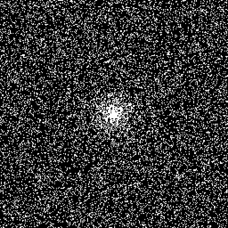
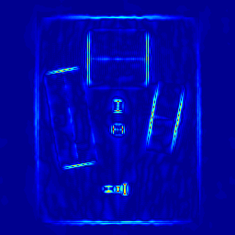
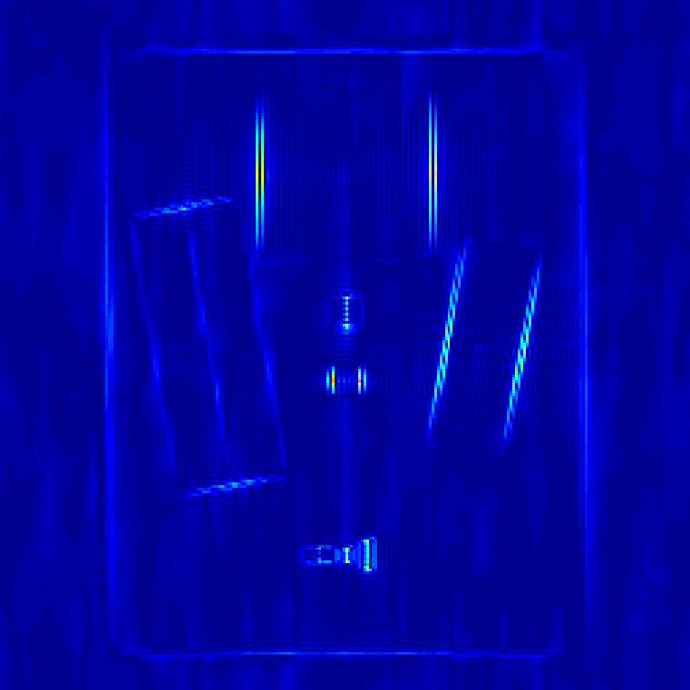
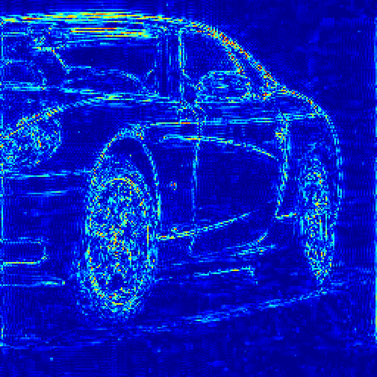
Throughout the experiments, we test two synthetic images (“Ellipses” and “Rectangles”), and two natural images (“Airplane”, and “Car”) taking the values in [0,1][0,1], as shown in fig. 2. The data 𝒇{\boldsymbol{f}} is synthesized by randomly sampling 20%20\% of 256×256256\times 256 Fourier samples via the variable density sampling method described in [47]. A complex white Gaussian noise with the standard deviation 11 is also added to generate a noisy partial sampling. For eqs. 4.1, 4.2 and 4.3, we use the K×KK\times K square patch for simplicity. Specifically, we choose K=31K=31 for the “Ellipses”, K=25K=25 for the “Rectangles”, and K=51K=51 for “Airplane” and “Car”, depending on the geometry of the target images. More precisely, in eqs. 4.1, 4.2 and 4.3, we use the discrete Fourier transform of the images restored by the TGV model eq. 4.5 and the inf-convolution model eq. 4.6 respectively, to compute the SVDs of multi-fold Hankel matrices using the K×KK\times K patches, which will be used for 𝓦k{\boldsymbol{{\mathcal{W}}}}_{k}’s in eq. 4.1 and initializations in eqs. 4.2 and 4.3. For eq. 4.4, we choose 𝓦{\boldsymbol{{\mathcal{W}}}} to be the undecimated tensor product piecewise linear B-spline framelet transform with 11 level of decomposition [26]. For eqs. 4.5 and 4.6, we use the forward difference with the periodic boundary condition for the difference operators ∇\boldsymbol{\nabla}, ∇s\boldsymbol{\nabla}_{s}, and ∇2\boldsymbol{\nabla}^{2}. In all of the experiments, we have manually tuned the regularization parameters to achieve the optimal restoration results in each scenario. For the quantitative comparison, we compute the signal-to-noise ratio (SNR), the high frequency error norm (HFEN) [59], and the structure similarity index map (SSIM) [64]. Note that for eqs. 4.1, 4.2 and 4.3, the restored image is computed via the inverse DFT of the restored Fourier samples.

Refer to caption
(a) Ellipses
Refer to caption
(b) Rectangles
Refer to caption
(c) Airplane
Refer to caption
(d) Car
Refer to caption
(e) Ellipses-observed
Refer to caption
(f) Rectangles-observed
Refer to caption
(g) Airplane-observed
Refer to caption
(h) Car-observed
Figure 2: Visualization of test images and observed images. All images are displayed in the window level [0,1][0,1] for the fair comparisons.
Images Indices Zero fill Model eq. 4.1 SLRM eq. 4.2 GSLR eq. 4.3 Fra eq. 4.4 TGV eq. 4.5 IF eq. 4.6
Ellipses SNR 13.7513.75 36.13 32.1832.18 30.9330.93 27.4127.41 29.6729.67 28.3628.36
HFEN 0.77460.7746 0.0375 0.07130.0713 0.07890.0789 0.15330.1533 0.10290.1029 0.13510.1351
SSIM 0.41620.4162 0.9943 0.97840.9784 0.97460.9746 0.89660.8966 0.95470.9547 0.93350.9335
Rectangles SNR 15.6815.68 35.00 30.7430.74 30.4230.42 24.3024.30 29.2829.28 27.4327.43
HFEN 0.79140.7914 0.0876 0.14560.1456 0.17700.1770 0.44440.4444 0.18780.1878 0.23660.2366
SSIM 0.61300.6130 0.9803 0.9815 0.97420.9742 0.93910.9391 0.95520.9552 0.92110.9211
Airplane SNR 21.5521.55 36.23 33.8433.84 33.1233.12 31.2431.24 33.4033.40 32.9232.92
HFEN 0.44020.4402 0.0530 0.07240.0724 0.07530.0753 0.11350.1135 0.08030.0803 0.08890.0889
SSIM 0.73860.7386 0.9822 0.97060.9706 0.96930.9693 0.95640.9564 0.96690.9669 0.96380.9638
Car SNR 15.8815.88 27.42 25.8825.88 24.8124.81 22.7222.72 25.6925.69 25.1625.16
HFEN 0.55280.5528 0.1057 0.14470.1447 0.14600.1460 0.22900.2290 0.15300.1530 0.16690.1669
SSIM 0.56270.5627 0.9569 0.92910.9291 0.92820.9282 0.87610.8761 0.92180.9218 0.91120.9112
Table 1: Comparison of SNRs, HFENs, and SSIMs.

table 1 summarizes the SNR, the HFEN, and the SSIM of the aforementioned approaches. figs. 3, 4, 5 and 6 display the visual comparisons (the first row) together with the zoom-in views (the second row) and the error maps (the third row) of eq. 4.1 against eqs. 4.4, 4.5, 4.6, 4.2 and 4.3. Throughout this paper, all restored images are displayed in the window level [0,1][0,1], and all error maps are displayed in the window level [0,0.2][0,0.2] for fair comparisons. We can see that the relaxed model eq. 4.1 consistently performs best, and the SLRM model eq. 4.2 performs the second in almost every index in all scenarios, and the improvements are visually observable as well, both of which demonstrate that our proposed SLRM framework performs well in the piecewise smooth image restoration.

At first glance, since the models eqs. 4.1 and 4.2 can be regarded as different relaxations of the structured low rank matrix framework for the continuous domain regularization, the results also suggest that the off-the-grid regularization performs better than the on-the-grid regularization as it can reduce the basis mismatch between the true support (or the true singularity) in continuum and the discrete grid, leading to the improvements in the indices. In fact, due to such a basis mismatch, the conventional on-the-grid approaches (eqs. 4.4, 4.5 and 4.6) suffers from the errors concentrated near the image singularities as well as the distorted shapes compared to eq. 4.1, which can be seen in the error maps and the zoom-in views of figs. 3, 4, 5 and 6.

Most importantly, the numerical results illustrate the followings. First of all, from the comparisons between eqs. 4.2 and 4.3, we can see that the proposed SLRM framework performs better than the GSLR framework in [39] for the piecewise smooth image restoration. Second, from the comparisons between eqs. 4.1 and 4.2, we can further see that the relaxation into the wavelet frame analysis approach can achieve further improvements over the direct rank minimization. As previously mentioned, since the proposed SLRM framework takes the GSLR framework in [39] as a special case, we can restore broader range of piecewise smooth images. In addition, it should be noted that the annihilation of the Fourier samples of the second order derivatives in general require larger annihilating filter than the first order derivatives [50], which may degrade the low rank structures of the corresponding multi-fold Hankel matrix. As a consequence, the GSLR framework can introduce staircase artifacts in the smooth region compared to the proposed SLRM framework, as can be seen in the zoom-in views of figs. 3, 4, 5 and 6. Finally, since the weights corresponding to the derivatives in the image domain amplifies the noise in the high frequencies, it is likely that the direct rank minimization approaches (eqs. 4.2 and 4.3) lead to the artifacts near the image singularities corresponding to the high frequency components, whereas the relaxation into the wavelet frame analysis approach (eq. 4.1) can achieve the denoising effect in spite of the amplified noise, leading to the better restoration results with less artifacts near the edges, as can be seen in the error maps in figs. 3, 4, 5 and 6.

Refer to caption
(a)
Refer to caption
(b)
Refer to caption
(c)
Refer to caption
(d)
Refer to caption
(e)
Refer to caption
(f)
Refer to caption
(g)
Refer to caption
(h)
Refer to caption
(i)
Refer to caption
(j)
Refer to caption
(k)
Refer to caption
(l)
Refer to caption
(m)
Refer to caption
(n)
Refer to caption
(o)
Refer to caption
(p)
Refer to caption
(q)
Refer to caption
(r)
Refer to caption
(s)
Refer to caption
(t)
Refer to caption
(u)
Figure 3: Visual comparisons for “Ellipses”. fig. 3a: original image, fig. 3b: model eq. 4.1, fig. 3c: SLRM eq. 4.2, fig. 3d: GSLR eq. 4.3, fig. 3e: framelet eq. 4.4, fig. 3f: TGV eq. 4.5, fig. 3g: infimal convolution eq. 4.6. figs. 3h, 3i, 3j, 3k, 3l, 3m and 3n: zoom-in views of figs. 3a, 3b, 3c, 3d, 3e, 3f and 3g. Yellow arrows indicate the region worth noting for comparisons among eqs. 4.1, 4.2 and 4.3, and red arrows indicate the region worth noting for comparisons among eqs. 4.1, 4.4, 4.5 and 4.6. fig. 3o: sample region, figs. 3p, 3q, 3r, 3s, 3t and 3u: error maps of figs. 3b, 3c, 3d, 3e, 3f and 3g.
Refer to caption
(a)
Refer to caption
(b)
Refer to caption
(c)
Refer to caption
(d)
Refer to caption
(e)
Refer to caption
(f)
Refer to caption
(g)
Refer to caption
(h)
Refer to caption
(i)
Refer to caption
(j)
Refer to caption
(k)
Refer to caption
(l)
Refer to caption
(m)
Refer to caption
(n)
Refer to caption
(o)
Refer to caption
(p)
Refer to caption
(q)
Refer to caption
(r)
Refer to caption
(s)
Refer to caption
(t)
Refer to caption
(u)
Figure 4: Visual comparisons for “Rectangles”. fig. 4a: original image, fig. 4b: model eq. 4.1, fig. 4c: SLRM eq. 4.2, fig. 4d: GSLR eq. 4.3, fig. 4e: framelet eq. 4.4, fig. 4f: TGV eq. 4.5, fig. 4g: infimal convolution eq. 4.6. figs. 4h, 4i, 4j, 4k, 4l, 4m and 4n: zoom-in views of figs. 4a, 4b, 4c, 4d, 4e, 4f and 4g. Red arrows indicate the region worth noting. fig. 4o: sample region, figs. 4p, 4q, 4r, 4s, 4t and 4u: error maps of figs. 4b, 4c, 4d, 4e, 4f and 4g.
Refer to caption
(a)
Refer to caption
(b)
Refer to caption
(c)
Refer to caption
(d)
Refer to caption
(e)
Refer to caption
(f)
Refer to caption
(g)
Refer to caption
(h)
Refer to caption
(i)
Refer to caption
(j)
Refer to caption
(k)
Refer to caption
(l)
Refer to caption
(m)
Refer to caption
(n)
Refer to caption
(o)
Refer to caption
(p)
Refer to caption
(q)
Refer to caption
(r)
Refer to caption
(s)
Refer to caption
(t)
Refer to caption
(u)
Figure 5: Visual comparisons for “Airplane”. fig. 5a: original image, fig. 5b: model eq. 4.1, fig. 5c: SLRM eq. 4.2, fig. 5d: GSLR eq. 4.3, fig. 5e: framelet eq. 4.4, fig. 5f: TGV eq. 4.5, fig. 5g: infimal convolution eq. 4.6. figs. 5h, 5i, 5j, 5k, 5l, 5m and 5n: zoom-in views of figs. 5a, 5b, 5c, 5d, 5e, 5f and 5g. Red arrows indicate the region worth noting. fig. 5o: sample region, figs. 5p, 5c, 5d, 5s, 5t, 5u, 5q and 5r: error maps of figs. 5b, 5e, 5f and 5g.
Refer to caption
(a)
Refer to caption
(b)
Refer to caption
(c)
Refer to caption
(d)
Refer to caption
(e)
Refer to caption
(f)
Refer to caption
(g)
Refer to caption
(h)
Refer to caption
(i)
Refer to caption
(j)
Refer to caption
(k)
Refer to caption
(l)
Refer to caption
(m)
Refer to caption
(n)
Refer to caption
(o)
Refer to caption
(p)
Refer to caption
(q)
Refer to caption
(r)
Refer to caption
(s)
Refer to caption
(t)
Refer to caption
(u)
Figure 6: Visual comparisons for “Car”. fig. 6a: original image, fig. 6b: model eq. 4.1, fig. 6c: SLRM eq. 4.2, fig. 6d: GSLR eq. 4.3, fig. 6e: framelet eq. 4.4, fig. 6f: TGV eq. 4.5, fig. 6g: infimal convolution eq. 4.6. figs. 6h, 6i, 6j, 6k, 6l, 6m and 6n: zoom-in views of figs. 6a, 6b, 6c, 6d, 6e, 6f and 6g. Red arrows indicate the region worth noting. fig. 6o: sample region, figs. 6p, 6q, 6r, 6s, 6t and 6u: error maps of figs. 6b, 6c, 6d, 6e, 6f and 6g.

5 Conclusion and future directions

In this paper, we have introduced a new structured low rank matrix framework for the piecewise smooth image restoration. Following the previous structured low rank matrix framework for the piecewise constant image [52], we assume that the image singularities lie in the zero level set of a band-limited periodic function. Inspired by the total generalized variation [7], we derive the annihilation relation of the Fourier samples of the gradient and the (symmetric) gradient tensor, which in turn leads to the low rank multi-fold Hankel matrices to balance between the first order derivatives and the second order derivatives. In addition, as a by-product of the proposed structured low rank matrix framework, we further introduce a wavelet frame based sparse regularization model for the piecewise image restoration via the continuous domain regularization, from the SVDs of low rank multi-fold Hankel matrices. Finally, the numerical experiments show that the proposed wavelet frame based model based on the proposed SLRM framework outperforms both the conventional on-the-grid approaches and the existing the SLRM framework as well as the existing rank minimization approaches for the piecewise smooth image restoration.

For the future work, we plan to generalize the frameworks in [52] to the piecewise smooth image restoration. More precisely, we need to develop sampling guarantees for the unique restoration of a continuous domain piecewise smooth image from its uniform low pass Fourier samples, based on the proposed annihilation relations. Unfortunately, it is not clear for us at this moment under what conditions we can restore the singularity set from uniform Fourier samples as the annihilation relations involve a blind deconvolution problem due to the additional unknown vector field pp in theorem 2.1. Nevertheless, this is definitely a future direction we would like to work on. We are also interested in proving the restoration guarantee of eq. 3.2 (or its convex nuclear norm relaxation) given that 𝓐=𝓡𝕄{\boldsymbol{{\mathcal{A}}}}={\boldsymbol{{\mathcal{R}}}}_{{\mathbb{M}}}, i.e. the sample grid 𝕄{\mathbb{M}} is drawn from the image grid 𝕆{\mathbb{O}} uniformly at random, which generalizes the theoretical frameworks in [49] to the piecewise smooth image restoration.

Finally, to broaden the scope of applications, it is also likely to apply the idea in this paper to the various image restoration tasks such as the blind deconvolution (especially that in the frequency domain which is related to the retinex [46]) and the sparse angle CT. In fact, it is not clear at this moment how to extend this approach to the sparse angle CT restoration, as the measurement can be viewed as the Fourier samples on the discrete radial grid. Nevertheless, this is also an important future work for the broader scope of applications. Finally, observing the successive structure in our SLRM framework, we are also interested in developing a deep learning framework, motivated by the recent works on the deep learning techniques combined with the structured low rank matrix approaches [40, 43, 56, 57].

Appendix A Preliminaries on tight wavelet frames

Provided here is a brief introduction on tight wavelet frames and the wavelet frame based image restoration. Interested readers may consult [9, 26, 27, 60, 62] for detailed surveys on tight wavelet frames, and [11] for detailed reviews on the wavelet frame based image restoration. For the sake of simplicity, we only discuss the real valued wavelet tight frame systems, but note that it is not difficult to extend the idea to the complex case.

Let ℋ{\mathscr{H}} be a Hilbert space equipped with an inner product ⟨⋅,⋅⟩\langle\cdot,\cdot\rangle. A (Bessel) sequence {𝝋n:n∈ℤ}⊆ℋ\{\boldsymbol{\varphi}_{n}:n\in{\mathbb{Z}}\}\subseteq{\mathscr{H}} is called a tight frame on ℋ{\mathscr{H}} if

‖𝒖‖2=∑n∈ℤ|⟨𝒖,𝝋n⟩|2for all​𝒖∈ℋ.\displaystyle\|\boldsymbol{u}\|^{2}=\sum_{n\in{\mathbb{Z}}}|\langle\boldsymbol{u},\boldsymbol{\varphi}_{n}\rangle|^{2}~~~~~\text{for all}~~~\boldsymbol{u}\in{\mathscr{H}}. (A.1)

Given {𝝋n:n∈ℤ}⊆ℋ\{\boldsymbol{\varphi}_{n}:n\in{\mathbb{Z}}\}\subseteq{\mathscr{H}}, we define the analysis operator 𝓦:ℋ→ℓ2​(ℤ){\boldsymbol{{\mathcal{W}}}}:{\mathscr{H}}\to\ell_{2}({\mathbb{Z}}) as

𝒖∈ℋ↦𝓦​𝒖={⟨𝒖,𝝋n⟩:n∈ℤ}∈ℓ2​(ℤ).\displaystyle\boldsymbol{u}\in{\mathscr{H}}\mapsto{\boldsymbol{{\mathcal{W}}}}\boldsymbol{u}=\{\langle\boldsymbol{u},\boldsymbol{\varphi}_{n}\rangle:n\in{\mathbb{Z}}\}\in\ell_{2}({\mathbb{Z}}).

The synthesis operator 𝓦T:ℓ2​(ℤ)→ℋ{\boldsymbol{{\mathcal{W}}}}^{T}:\ell_{2}({\mathbb{Z}})\to{\mathscr{H}} is defined as the adjoint of 𝓦{\boldsymbol{{\mathcal{W}}}}:

𝒄∈ℓ2​(ℤ)↦𝓦T​𝒄=∑n∈ℤ𝒄⁡(n)​𝝋n∈ℋ.\displaystyle{\boldsymbol{c}}\in\ell_{2}({\mathbb{Z}})\mapsto{\boldsymbol{{\mathcal{W}}}}^{T}{\boldsymbol{c}}=\sum_{n\in{\mathbb{Z}}}{\boldsymbol{c}}(n)\boldsymbol{\varphi}_{n}\in{\mathscr{H}}.

Then {𝝋n:n∈ℤ}\{\boldsymbol{\varphi}_{n}:n\in{\mathbb{Z}}\} is a tight frame on ℋ{\mathscr{H}} if and only if 𝓦T​𝓦=𝓘{\boldsymbol{{\mathcal{W}}}}^{T}{\boldsymbol{{\mathcal{W}}}}={\boldsymbol{{\mathcal{I}}}}. It follows that, for a given tight frame {𝝋n:n∈ℤ}\{\boldsymbol{\varphi}_{n}:n\in{\mathbb{Z}}\}, we have the following canonical expression:

𝒖=∑n∈ℤ⟨𝒖,𝝋n⟩​𝝋n,\displaystyle\boldsymbol{u}=\sum_{n\in{\mathbb{Z}}}\langle\boldsymbol{u},\boldsymbol{\varphi}_{n}\rangle\boldsymbol{\varphi}_{n},

with 𝓦​𝒖={⟨𝒖,𝝋n⟩:n∈ℤ}{\boldsymbol{{\mathcal{W}}}}\boldsymbol{u}=\{\langle\boldsymbol{u},\boldsymbol{\varphi}_{n}\rangle:n\in{\mathbb{Z}}\} being called the canonical tight frame coefficients. Hence, the tight frames are extensions of orthonormal bases to the redundant systems. In fact, a tight frame is an orthonormal basis if and only if ‖𝝋n‖=1\|\boldsymbol{\varphi}_{n}\|=1 for all n∈ℤn\in{\mathbb{Z}}.

One of the most widely used class of tight frames is the discrete wavelet frame generated by a set of finitely supported filters {𝒂1,⋯,𝒂m}\{{\boldsymbol{a}}_{1},\cdots,{\boldsymbol{a}}_{m}\}. Throughout this paper, we only discuss the two dimensional undecimated wavelet frames on ℓ2​(ℤ2)\ell_{2}({\mathbb{Z}}^{2}), but note that it is not difficult to extend to ℓ2​(ℤd)\ell_{2}({\mathbb{Z}}^{d}) with d≥3d\geq 3. For 𝒂∈ℓ1​(ℤ2){\boldsymbol{a}}\in\ell_{1}({\mathbb{Z}}^{2}), define a convolution operator 𝓢𝒂:ℓ2​(ℤ2)→ℓ2​(ℤ2){\boldsymbol{{\mathcal{S}}}}_{{\boldsymbol{a}}}:\ell_{2}({\mathbb{Z}}^{2})\to\ell_{2}({\mathbb{Z}}^{2}) by

(𝓢𝒂​𝒖)​(𝒌)=(𝒂∗𝒖)​(𝒌)=∑𝒍∈ℤ2𝒂⁡(𝒌−𝒍)​𝒖​(𝒍)for​𝒖∈ℓ2​(ℤ2).\displaystyle({\boldsymbol{{\mathcal{S}}}}_{{\boldsymbol{a}}}\boldsymbol{u})({\boldsymbol{k}})=({\boldsymbol{a}}\ast\boldsymbol{u})({\boldsymbol{k}})=\sum_{{\boldsymbol{l}}\in{\mathbb{Z}}^{2}}{\boldsymbol{a}}({\boldsymbol{k}}-{\boldsymbol{l}})\boldsymbol{u}({\boldsymbol{l}})~~~~~\text{for}~~~\boldsymbol{u}\in\ell_{2}({\mathbb{Z}}^{2}). (A.2)

Given a set of finitely supported filters {𝒂1,⋯,𝒂m}\{{\boldsymbol{a}}_{1},\cdots,{\boldsymbol{a}}_{m}\}, define the analysis operator 𝓦{\boldsymbol{{\mathcal{W}}}} and the synthesis operator 𝓦T{\boldsymbol{{\mathcal{W}}}}^{T} by

𝓦\displaystyle{\boldsymbol{{\mathcal{W}}}} =[𝓢𝒂1(−⋅)T,𝓢𝒂2(−⋅)T,⋯,𝓢𝒂m(−⋅)T]T,\displaystyle=\left[{\boldsymbol{{\mathcal{S}}}}_{{\boldsymbol{a}}_{1}(-\cdot)}^{T},{\boldsymbol{{\mathcal{S}}}}_{{\boldsymbol{a}}_{2}(-\cdot)}^{T},\cdots,{\boldsymbol{{\mathcal{S}}}}_{{\boldsymbol{a}}_{m}(-\cdot)}^{T}\right]^{T}, (A.3)
𝓦T\displaystyle{\boldsymbol{{\mathcal{W}}}}^{T} =[𝓢𝒂1,𝓢𝒂2,⋯,𝓢𝒂m],\displaystyle=\big[{\boldsymbol{{\mathcal{S}}}}_{{\boldsymbol{a}}_{1}},{\boldsymbol{{\mathcal{S}}}}_{{\boldsymbol{a}}_{2}},\cdots,{\boldsymbol{{\mathcal{S}}}}_{{\boldsymbol{a}}_{m}}\big], (A.4)

respectively. Then, the direct computation can show that the rows of 𝓦{\boldsymbol{{\mathcal{W}}}} form a tight frame on ℓ2​(ℤ2)\ell_{2}({\mathbb{Z}}^{2}) (i.e. 𝓦T​𝓦=𝓘{\boldsymbol{{\mathcal{W}}}}^{T}{\boldsymbol{{\mathcal{W}}}}={\boldsymbol{{\mathcal{I}}}}) if and only if the filters {𝒂1,⋯,𝒂m}\{{\boldsymbol{a}}_{1},\cdots,{\boldsymbol{a}}_{m}\} satisfy

∑j=1m∑𝒍∈ℤ2𝒂j​(𝒌+𝒍)​𝒂j​(𝒍)=𝜹⁡(𝒌)={1if​𝒌=𝟎,0if​𝒌≠𝟎,\displaystyle\sum_{j=1}^{m}\sum_{{\boldsymbol{l}}\in{\mathbb{Z}}^{2}}{\boldsymbol{a}}_{j}({\boldsymbol{k}}+{\boldsymbol{l}}){\boldsymbol{a}}_{j}({\boldsymbol{l}})=\boldsymbol{\delta}({\boldsymbol{k}})=\left\{\begin{array}[]{cl}1&\text{if}~{\boldsymbol{k}}={\mathbf{0}},\\ 0&\text{if}~{\boldsymbol{k}}\neq{\mathbf{0}},\end{array}\right.

called the unitary extension principle (UEP) condition [37]. Finally, for a two dimensional discrete image on the finite grid, 𝓢𝒂{\boldsymbol{{\mathcal{S}}}}_{{\boldsymbol{a}}} in eq. A.2 with a finitely supported 𝒂{\boldsymbol{a}} denotes the discrete convolution under the periodic boundary condition throughout this paper.

For the image restoration, we assume that there exists a tight wavelet frame 𝓦{\boldsymbol{{\mathcal{W}}}} defined as eq. A.3 with filters {𝒂1,⋯,𝒂m}\left\{{\boldsymbol{a}}_{1},\cdots,{\boldsymbol{a}}_{m}\right\} such that 𝒖\boldsymbol{u} is sparse under 𝓦{\boldsymbol{{\mathcal{W}}}}. This leads us to solve

min𝒄⁡12​‖𝓐​𝓦T​𝒄−𝒇‖22+12​‖(𝓘−𝓦​𝓦T)​𝒄‖22+‖𝜸⋅𝒄‖1\displaystyle\min_{{\boldsymbol{c}}}\frac{1}{2}\|{\boldsymbol{{\mathcal{A}}}}{\boldsymbol{{\mathcal{W}}}}^{T}{\boldsymbol{c}}-{\boldsymbol{f}}\|_{2}^{2}+\frac{1}{2}\|({\boldsymbol{{\mathcal{I}}}}-{\boldsymbol{{\mathcal{W}}}}{\boldsymbol{{\mathcal{W}}}}^{T}){\boldsymbol{c}}\|_{2}^{2}+\|\boldsymbol{\gamma}\cdot{\boldsymbol{c}}\|_{1} (A.7)

and restore 𝒖=𝓦T​𝒄\boldsymbol{u}={\boldsymbol{{\mathcal{W}}}}^{T}{\boldsymbol{c}}. In eq. A.7, the first term is a data fidelity term, the third ℓ1\ell_{1} norm is defined as

‖𝜸⋅𝒄‖1=∑j=1mγj​‖𝒄j‖1\displaystyle\|\boldsymbol{\gamma}\cdot{\boldsymbol{c}}\|_{1}=\sum_{j=1}^{m}\gamma_{j}\left\|{\boldsymbol{c}}_{j}\right\|_{1} (A.8)

with the parameters 𝜸=[γ1,…,γm]T\boldsymbol{\gamma}=\left[\gamma_{1},\ldots,\gamma_{m}\right]^{T} and γj>0\gamma_{j}>0, to promote the sparsity of 𝒄{\boldsymbol{c}}. The second term penalizes the distance between 𝒄{\boldsymbol{c}} and its projection onto ℛ⁡(𝓦){\mathscr{R}}({\boldsymbol{{\mathcal{W}}}}). Since we obtain the image via 𝒖=𝓦T​𝒄\boldsymbol{u}={\boldsymbol{{\mathcal{W}}}}^{T}{\boldsymbol{c}}, the second term in fact forces the sparse coefficient 𝒄{\boldsymbol{c}} close to the canonical coefficient of the restored image. Since the magnitude/decay of the canonical coefficient reflects the regularity of the image under some mild conditions on the tight frame system 𝓦{\boldsymbol{{\mathcal{W}}}} [4], we can see that the second and third terms promote a balance between the sparsity of coefficient and the regularity of image.

We can further impose the flexibility on eq. A.7 by introducing the weight on the second term:

min𝒄⁡12​‖𝓐​𝓦T​𝒄−𝒇‖22+μ2​‖(𝓘−𝓦​𝓦T)​𝒄‖22+‖𝜸⋅𝒄‖1,\displaystyle\min_{{\boldsymbol{c}}}\frac{1}{2}\|{\boldsymbol{{\mathcal{A}}}}{\boldsymbol{{\mathcal{W}}}}^{T}{\boldsymbol{c}}-{\boldsymbol{f}}\|_{2}^{2}+\frac{\mu}{2}\|({\boldsymbol{{\mathcal{I}}}}-{\boldsymbol{{\mathcal{W}}}}{\boldsymbol{{\mathcal{W}}}}^{T}){\boldsymbol{c}}\|_{2}^{2}+\|\boldsymbol{\gamma}\cdot{\boldsymbol{c}}\|_{1}, (A.9)

called the balanced approach [9, 21]. If μ=0\mu=0, then eq. A.9 becomes the synthesis approach [25, 29, 31]

min𝒄⁡12​‖𝓐​𝓦T​𝒄−𝒇‖22+‖𝜸⋅𝒄‖1,\displaystyle\min_{{\boldsymbol{c}}}\frac{1}{2}\|{\boldsymbol{{\mathcal{A}}}}{\boldsymbol{{\mathcal{W}}}}^{T}{\boldsymbol{c}}-{\boldsymbol{f}}\|_{2}^{2}+\|\boldsymbol{\gamma}\cdot{\boldsymbol{c}}\|_{1}, (A.10)

as we aim to find the sparsest coefficient that synthesizes the image. On the other hand, if μ=∞\mu=\infty, then it must be (𝓘−𝓦​𝓦T)​𝒄=𝟎({\boldsymbol{{\mathcal{I}}}}-{\boldsymbol{{\mathcal{W}}}}{\boldsymbol{{\mathcal{W}}}}^{T}){\boldsymbol{c}}={\mathbf{0}}. Since we then have 𝒄∈ℛ⁡(𝓦){\boldsymbol{c}}\in{\mathscr{R}}({\boldsymbol{{\mathcal{W}}}}), it follows that 𝒄=𝓦​𝒖{\boldsymbol{c}}={\boldsymbol{{\mathcal{W}}}}\boldsymbol{u} for some 𝒖\boldsymbol{u}. Hence, eq. A.7 becomes the analysis approach [13]

min𝒖⁡12​‖𝓐​𝒖−𝒇‖22+‖𝜸⋅𝓦​𝒖‖1.\displaystyle\min_{\boldsymbol{u}}\frac{1}{2}\|{\boldsymbol{{\mathcal{A}}}}\boldsymbol{u}-{\boldsymbol{f}}\|_{2}^{2}+\|\boldsymbol{\gamma}\cdot{\boldsymbol{{\mathcal{W}}}}\boldsymbol{u}\|_{1}. (A.11)

Since the analysis approach promotes the sparse canonical coefficient, it emphasizes the regularity of the restored image.

These three approaches are equivalent if and only if 𝓦T​𝓦=𝓦​𝓦T=𝓘{\boldsymbol{{\mathcal{W}}}}^{T}{\boldsymbol{{\mathcal{W}}}}={\boldsymbol{{\mathcal{W}}}}{\boldsymbol{{\mathcal{W}}}}^{T}={\boldsymbol{{\mathcal{I}}}}, i.e. 𝓦{\boldsymbol{{\mathcal{W}}}} forms an orthonormal basis. However, since we consider the redundant system, each approach will lead to the different restoration results. Notice that the coefficient vector 𝒄{\boldsymbol{c}} obtained from the synthesis approach eq. A.10 is much sparser than the canonical coefficient 𝓦​𝒖{\boldsymbol{{\mathcal{W}}}}\boldsymbol{u} obtained from the analysis approach eq. A.11. It is empirically observed that the synthesis approach eq. A.10 tends to yield some artifacts in the restored image. In contrast, the analysis approach eq. A.11 usually have less artifacts as it promotes the regularity of the image along the singularities. Theoretically, it has been proved in [11] that, under a suitable choice of parameters, the analysis approach eq. A.11 can be seen as sophisticated discretization of a variational model including the Rudin-Osher-Fatemi model [61], which enables a geometric interpretation on eq. A.11.

Appendix B Proof of theorem 2.1

Let u⁡(𝒙)u(\boldsymbol{x}) be defined as in eq. 2.12 where the singularity curves Γ=⋃j=1J∂Ωj\Gamma=\bigcup_{j=1}^{J}\partial\Omega_{j} satisfy eq. 2.14. In the sense of distribution, the gradient of uu satisfies

∇u​(𝒙)=(∂1u⁡(𝒙),∂2u⁡(𝒙))=∑j=1J(𝜶j​1Ωj​(𝒙)+(𝜶jT​𝒙+βj)​𝒏j​(𝒙)​d​𝝈​(𝒙)|∂Ωj)\displaystyle\nabla u(\boldsymbol{x})=\left(\partial_{1}u(\boldsymbol{x}),\partial_{2}u(\boldsymbol{x})\right)=\sum_{j=1}^{J}\left(\boldsymbol{\alpha}_{j}1_{\Omega_{j}}(\boldsymbol{x})+\left(\boldsymbol{\alpha}_{j}^{T}\boldsymbol{x}+\beta_{j}\right)\boldsymbol{n}_{j}(\boldsymbol{x})\mathrm{d}\boldsymbol{\sigma}(\boldsymbol{x})\big|_{\partial\Omega_{j}}\right) (B.1)

where 𝒏j=(nj​1,nj​2)\boldsymbol{n}_{j}=\left(n_{j1},n_{j2}\right) is the outward normal vector on ∂Ωj\partial\Omega_{j}, and 𝝈\boldsymbol{\sigma} is the surface measure. We define

p⁡(𝒙)=(p1​(𝒙),p2​(𝒙))=∑j=1J𝜶j​1Ωj​(𝒙)\displaystyle p(\boldsymbol{x})=\left(p_{1}(\boldsymbol{x}),p_{2}(\boldsymbol{x})\right)=\sum_{j=1}^{J}\boldsymbol{\alpha}_{j}1_{\Omega_{j}}(\boldsymbol{x})

and

d​𝝂​(𝒙)=∑j=1Jd​𝝂j​(𝒙)=∑j=1J(𝜶jT​𝒙+βj​𝒏j​(𝒙)​d​𝝈​(𝒙)|∂Ωj).\displaystyle\mathrm{d}\boldsymbol{\nu}(\boldsymbol{x})=\sum_{j=1}^{J}\mathrm{d}\boldsymbol{\nu}_{j}(\boldsymbol{x})=\sum_{j=1}^{J}\left(\boldsymbol{\alpha}_{j}^{T}\boldsymbol{x}+\beta_{j}\boldsymbol{n}_{j}(\boldsymbol{x})\mathrm{d}\boldsymbol{\sigma}(\boldsymbol{x})\big|_{\partial\Omega_{j}}\right).

Then it is obvious that we have

∇u−p=d​𝝂=∑j=1Jd​𝝂j.\displaystyle\nabla u-p=\mathrm{d}\boldsymbol{\nu}=\sum_{j=1}^{J}\mathrm{d}\boldsymbol{\nu}_{j}. (B.2)

Since |𝒏j|=1|\boldsymbol{n}_{j}|=1 almost everywhere on ∂Ωj\partial\Omega_{j}, 𝜶jT​𝒙+βj\boldsymbol{\alpha}_{j}^{T}\boldsymbol{x}+\beta_{j} is continuous on a compact set ∂Ωj\partial\Omega_{j}, ∇u−p\nabla u-p in eq. B.2 defines a finite Radon vector measure on ℝ2{\mathbb{R}}^{2} supported on Γ\Gamma. In addition, since eq. B.1 as well as eq. B.2 holds in the sense of tempered distribution, we can compute ℱ​(∇u−p)​(𝝃){\mathscr{F}}(\nabla u-p)({\boldsymbol{\xi}}) as a Fourier transform of a measure (e.g. [32]). Namely, we have

ℱ(∇u−p)(𝝃)=∑j=1J∫∂Ωje−2πi𝝃⋅𝒙d𝝂j(𝒙).\displaystyle{\mathscr{F}}(\nabla u-p)({\boldsymbol{\xi}})=\sum_{j=1}^{J}\int_{\partial\Omega_{j}}e^{-2\pi i{\boldsymbol{\xi}}\cdot\boldsymbol{x}}\mathrm{d}\boldsymbol{\nu}_{j}(\boldsymbol{x}). (B.3)

Let φ∈𝒮\varphi\in{\mathscr{S}}, where 𝒮{\mathscr{S}} is the space of Schwartz functions (e.g. [32]). Then the direct computation shows that (ℱ​(∇u−p)∗φ^)​(𝝃)\left({\mathscr{F}}(\nabla u-p)\ast\widehat{\varphi}\right)({\boldsymbol{\xi}}) satisfies

(ℱ(∇u−p)∗φ^)(𝝃)=∑j=1J∫∂Ωje−2πi𝝃⋅𝒙φ(𝒙)d𝝂j(𝒙).\displaystyle\begin{split}\left({\mathscr{F}}(\nabla u-p)\ast\widehat{\varphi}\right)({\boldsymbol{\xi}})=\sum_{j=1}^{J}\int_{\partial\Omega_{j}}e^{-2\pi i{\boldsymbol{\xi}}\cdot\boldsymbol{x}}\varphi(\boldsymbol{x})\mathrm{d}\boldsymbol{\nu}_{j}(\boldsymbol{x}).\end{split} (B.4)

From eq. B.4, it is easy to see that if Γ\Gamma lies in the zero level set of φ\varphi, then ℱ⁡(∇u−p)∗φ^=0{\mathscr{F}}(\nabla u-p)\ast\widehat{\varphi}=0. In particular, if φ\varphi is defined as eq. 2.14, then

φ^​(𝝃)=∑𝒌∈𝕂𝒂⁡(𝒌)​δ​(𝝃+𝒌),\displaystyle\widehat{\varphi}({\boldsymbol{\xi}})=\sum_{{\boldsymbol{k}}\in{\mathbb{K}}}{\boldsymbol{a}}({\boldsymbol{k}})\delta({\boldsymbol{\xi}}+{\boldsymbol{k}}),

which leads to

(ℱ⁡(∇u−p)∗φ^)​(𝝃)=∑𝒌∈𝕂ℱ⁡(∇u−p)​(𝝃+𝒌)​𝒂​(𝒌)=0.\displaystyle\left({\mathscr{F}}(\nabla u-p)\ast\widehat{\varphi}\right)({\boldsymbol{\xi}})=\sum_{{\boldsymbol{k}}\in{\mathbb{K}}}{\mathscr{F}}(\nabla u-p)({\boldsymbol{\xi}}+{\boldsymbol{k}}){\boldsymbol{a}}({\boldsymbol{k}})=0.

This proves eq. 2.15.

To complete the proof, we further note that in the sense of distribution, ∇sp\nabla_{s}p satisfies

∇sp=−∑j=1J[αj​1​nj​112​(αj​1​nj​2+αj​2​nj​1)12​(αj​1​nj​2+αj​2​nj​1)αj​2​nj​2]d𝝈|∂Ωj:=∑j=1Jd𝚽j.\displaystyle\nabla_{s}p=-\sum_{j=1}^{J}\left[\begin{array}[]{cc}\alpha_{j1}n_{j1}&\displaystyle{\frac{1}{2}\left(\alpha_{j1}n_{j2}+\alpha_{j2}n_{j1}\right)}\\ \displaystyle{\frac{1}{2}\left(\alpha_{j1}n_{j2}+\alpha_{j2}n_{j1}\right)}&\alpha_{j2}n_{j2}\end{array}\right]\mathrm{d}\boldsymbol{\sigma}\big|_{\partial\Omega_{j}}:=\sum_{j=1}^{J}\mathrm{d}\boldsymbol{\Phi}_{j}.

Following the similar arguments, it is not difficult to verify that d​𝚽j\mathrm{d}\boldsymbol{\Phi}_{j} in appendix B defines a finite Radon tensor measure on ℝ2{\mathbb{R}}^{2} supported on Γ\Gamma. which means that ℱ⁡(∇sp){\mathscr{F}}(\nabla_{s}p) is defined as

ℱ(∇sp)(𝝃)=∑j=1J∫∂Ωje−2πi𝝃⋅𝒙d𝚽j(𝒙).\displaystyle{\mathscr{F}}(\nabla_{s}p)({\boldsymbol{\xi}})=\sum_{j=1}^{J}\int_{\partial\Omega_{j}}e^{-2\pi i{\boldsymbol{\xi}}\cdot\boldsymbol{x}}\mathrm{d}\boldsymbol{\Phi}_{j}(\boldsymbol{x}). (B.7)

Therefore, for φ∈𝒮\varphi\in{\mathscr{S}}, we again have

(ℱ(∇sp)∗φ^)(𝝃)=∑j=1J∫∂Ωje−2πi𝝃⋅𝒙φ(𝒙)d𝚽j(𝒙),\displaystyle\left({\mathscr{F}}(\nabla_{s}p)\ast\widehat{\varphi}\right)({\boldsymbol{\xi}})=\sum_{j=1}^{J}\int_{\partial\Omega_{j}}e^{-2\pi i{\boldsymbol{\xi}}\cdot\boldsymbol{x}}\varphi(\boldsymbol{x})\mathrm{d}\boldsymbol{\Phi}_{j}(\boldsymbol{x}),

and in particular, for φ\varphi satisfying eq. 2.14, we have

(ℱ⁡(∇sp)∗φ^)​(𝝃)=∑𝒌∈𝕂ℱ⁡(∇sp)​(𝝃+𝒌)​𝒂​(𝒌)=0,\displaystyle\left({\mathscr{F}}(\nabla_{s}p)\ast\widehat{\varphi}\right)({\boldsymbol{\xi}})=\sum_{{\boldsymbol{k}}\in{\mathbb{K}}}{\mathscr{F}}(\nabla_{s}p)({\boldsymbol{\xi}}+{\boldsymbol{k}}){\boldsymbol{a}}({\boldsymbol{k}})=0,

and this completes the proof.

Appendix C Proof of theorem 3.7

Let u⁡(𝒙)u(\boldsymbol{x}) be a piecewise linear function defined as eq. 2.12, and 𝒗=ℱ⁡(u)|𝕆\boldsymbol{v}={\mathscr{F}}(u)\big|_{{\mathbb{O}}}. Assume eq. 3.13, and we consider the full SVDs

𝓗⁡(𝓓​𝒗−𝒒)\displaystyle{\boldsymbol{{\mathcal{H}}}}\left({\boldsymbol{{\mathcal{D}}}}\boldsymbol{v}-\boldsymbol{q}\right) =∑l=1M2𝚺1(l,l)𝑿1(:,l)(𝒀1(:,l))∗,\displaystyle=\sum_{l=1}^{M_{2}}\boldsymbol{\Sigma}_{1}^{(l,l)}{\boldsymbol{X}}_{1}^{(:,l)}\left({\boldsymbol{Y}}_{1}^{(:,l)}\right)^{*}, (C.1)

and

𝓗⁡(𝓔​𝒒)\displaystyle{\boldsymbol{{\mathcal{H}}}}\left({\boldsymbol{{\mathcal{E}}}}\boldsymbol{q}\right) =∑l=1M2𝚺2(l,l)𝑿2(:,l)(𝒀2(:,l))∗,\displaystyle=\sum_{l=1}^{M_{2}}\boldsymbol{\Sigma}_{2}^{(l,l)}{\boldsymbol{X}}_{2}^{(:,l)}\left({\boldsymbol{Y}}_{2}^{(:,l)}\right)^{*}, (C.2)

with

𝚺1(1,1)\displaystyle\boldsymbol{\Sigma}_{1}^{(1,1)} ≥⋯≥𝚺1(r1,r1)>0,and​𝚺1(l,l)=0​for​l>r1,\displaystyle\geq\cdots\geq\boldsymbol{\Sigma}_{1}^{(r_{1},r_{1})}>0,~~~\text{and}~~~\boldsymbol{\Sigma}_{1}^{(l,l)}=0~~\text{for}~~l>r_{1},

and

𝚺2(1,1)\displaystyle\boldsymbol{\Sigma}_{2}^{(1,1)} ≥⋯≥𝚺2(r1,r1)>0,and​𝚺2(l,l)=0​for​l>r2.\displaystyle\geq\cdots\geq\boldsymbol{\Sigma}_{2}^{(r_{1},r_{1})}>0,~~~\text{and}~~~\boldsymbol{\Sigma}_{2}^{(l,l)}=0~~\text{for}~~l>r_{2}.

Using the right singular vectors in eqs. C.1 and C.2, we define

𝒂1​l=M2−1/2𝒀1(:,l)and𝒂2​l=M2−1/2𝒀2(:,l)\displaystyle{\boldsymbol{a}}_{1l}=M_{2}^{-1/2}{\boldsymbol{Y}}_{1}^{(:,l)}~~~~~\text{and}~~~~~{\boldsymbol{a}}_{2l}=M_{2}^{-1/2}{\boldsymbol{Y}}_{2}^{(:,l)}

by reformulating M2×1M_{2}\times 1 vectors into K1×K2K_{1}\times K_{2} filters supported on 𝕂{\mathbb{K}}.

Firstly, we consider 𝒂11,…,𝒂1​M2{\boldsymbol{a}}_{11},\ldots,{\boldsymbol{a}}_{1M_{2}}. Note that we have

∑l=1M2(M2−1/2𝒀1(m,l))(M2−1/2𝒀¯1(n,l))=M2−1𝜹(m−n)={1if​m=n,0if​m≠n,\displaystyle\sum_{l=1}^{M_{2}}\left(M_{2}^{-1/2}{\boldsymbol{Y}}_{1}^{(m,l)}\right)\left(M_{2}^{-1/2}\overline{{\boldsymbol{Y}}}_{1}^{(n,l)}\right)=M_{2}^{-1}\boldsymbol{\delta}(m-n)=\left\{\begin{array}[]{cl}1&\text{if}~m=n,\\ 0&\text{if}~m\neq n,\end{array}\right.

for m,n=1,…,M2.m,n=1,\ldots,M_{2}. Then taking summation along the diagonals and rearranging into the two dimensional multi-indices, we can write appendix C as

∑l=1M2∑𝒎∈𝕂𝒂1​l​(𝒌+𝒎)​𝒂¯1​l​(𝒎)=𝜹⁡(𝒌)={1if​𝒌=𝟎,0if​𝒌≠𝟎.\displaystyle\sum_{l=1}^{M_{2}}\sum_{\boldsymbol{m}\in{\mathbb{K}}}{\boldsymbol{a}}_{1l}({\boldsymbol{k}}+\boldsymbol{m})\overline{{\boldsymbol{a}}}_{1l}(\boldsymbol{m})=\boldsymbol{\delta}({\boldsymbol{k}})=\left\{\begin{array}[]{cl}1&\text{if}~{\boldsymbol{k}}={\mathbf{0}},\\ 0&\text{if}~{\boldsymbol{k}}\neq{\mathbf{0}}.\end{array}\right.

This means that 𝓦1{\boldsymbol{{\mathcal{W}}}}_{1} and 𝓦1∗{\boldsymbol{{\mathcal{W}}}}_{1}^{*} defined as eqs. 3.11 and 3.12 using 𝒂11,…,𝒂1​M2{\boldsymbol{a}}_{11},\ldots,{\boldsymbol{a}}_{1M_{2}} satisfies

𝓦1∗𝓦1(𝓓𝒗−𝒒)=∑l=1M2𝓢𝒂¯1​l(𝓢𝒂1​l(−⋅)(𝓓𝒗−𝒒))=𝓓𝒗−𝒒,\displaystyle{\boldsymbol{{\mathcal{W}}}}_{1}^{*}{\boldsymbol{{\mathcal{W}}}}_{1}\left({\boldsymbol{{\mathcal{D}}}}\boldsymbol{v}-\boldsymbol{q}\right)=\sum_{l=1}^{M_{2}}{\boldsymbol{{\mathcal{S}}}}_{\overline{{\boldsymbol{a}}}_{1l}}\left({\boldsymbol{{\mathcal{S}}}}_{{\boldsymbol{a}}_{1l}(-\cdot)}\left({\boldsymbol{{\mathcal{D}}}}\boldsymbol{v}-\boldsymbol{q}\right)\right)={\boldsymbol{{\mathcal{D}}}}\boldsymbol{v}-\boldsymbol{q},

which shows that the filters 𝒂11,…,𝒂1​M2{\boldsymbol{a}}_{11},\ldots,{\boldsymbol{a}}_{1M_{2}} form a tight frame system.

In addition, we note that

𝚺1(l,l)𝑿1(:,l)=(𝓗(𝓓𝒗−𝒒))𝒀1(:,l)=(𝒀1(:,l)(−⋅)∗(𝓓𝒗−𝒒))|𝕆:𝕂\displaystyle\boldsymbol{\Sigma}_{1}^{(l,l)}{\boldsymbol{X}}_{1}^{(:,l)}=\left({\boldsymbol{{\mathcal{H}}}}\left({\boldsymbol{{\mathcal{D}}}}\boldsymbol{v}-\boldsymbol{q}\right)\right){\boldsymbol{Y}}_{1}^{(:,l)}=\left({\boldsymbol{Y}}_{1}^{(:,l)}(-\cdot)\ast\left({\boldsymbol{{\mathcal{D}}}}\boldsymbol{v}-\boldsymbol{q}\right)\right)\big|_{{\mathbb{O}}:{\mathbb{K}}}

where the discrete convolution ∗\ast is performed by reformulating 𝒀1(:,l)∈ℂM2{\boldsymbol{Y}}_{1}^{(:,l)}\in{\mathbb{C}}^{M_{2}} into a K1×K2K_{1}\times K_{2} filter supported on 𝕂{\mathbb{K}}. Then eq. C.1 implies that for l=r1+1,…,M2,l=r_{1}+1,\ldots,M_{2}, we have

(𝓢𝒂1​l(−⋅)(𝓓𝒗−𝒒))(𝒌)=0,𝒌∈𝕆:𝕂,\displaystyle\left({\boldsymbol{{\mathcal{S}}}}_{{\boldsymbol{a}}_{1l}(-\cdot)}\left({\boldsymbol{{\mathcal{D}}}}\boldsymbol{v}-\boldsymbol{q}\right)\right)({\boldsymbol{k}})=0,~~~~~{\boldsymbol{k}}\in{\mathbb{O}}:{\mathbb{K}},

which proves eqs. 3.14 and 3.16.

Similarly, we can prove that 𝒂21,…,𝒂2​M2{\boldsymbol{a}}_{21},\ldots,{\boldsymbol{a}}_{2M_{2}} satisfies

∑l=1M2∑𝒎∈𝕂𝒂2​l​(𝒌+𝒎)​𝒂¯2​l​(𝒎)=𝜹⁡(𝒌),\displaystyle\sum_{l=1}^{M_{2}}\sum_{\boldsymbol{m}\in{\mathbb{K}}}{\boldsymbol{a}}_{2l}({\boldsymbol{k}}+\boldsymbol{m})\overline{{\boldsymbol{a}}}_{2l}(\boldsymbol{m})=\boldsymbol{\delta}({\boldsymbol{k}}),

so that

𝓦2∗𝓦2(𝓔𝒒)=∑l=1M2𝓢𝒂¯2​l(𝓢𝒂2​l(−⋅)(𝓔𝒒))=𝓔𝒒.\displaystyle{\boldsymbol{{\mathcal{W}}}}_{2}^{*}{\boldsymbol{{\mathcal{W}}}}_{2}\left({\boldsymbol{{\mathcal{E}}}}\boldsymbol{q}\right)=\sum_{l=1}^{M_{2}}{\boldsymbol{{\mathcal{S}}}}_{\overline{{\boldsymbol{a}}}_{2l}}\left({\boldsymbol{{\mathcal{S}}}}_{{\boldsymbol{a}}_{2l}(-\cdot)}\left({\boldsymbol{{\mathcal{E}}}}\boldsymbol{q}\right)\right)={\boldsymbol{{\mathcal{E}}}}\boldsymbol{q}.

Finally, by eq. C.2, we have, for l=r2+1,…,M2l=r_{2}+1,\ldots,M_{2},

(𝓢𝒂2​l(−⋅)(𝓔𝒒))(𝒌)=0,𝒌∈𝕆:𝕂.\displaystyle\left({\boldsymbol{{\mathcal{S}}}}_{{\boldsymbol{a}}_{2l}(-\cdot)}\left({\boldsymbol{{\mathcal{E}}}}\boldsymbol{q}\right)\right)({\boldsymbol{k}})=0,~~~~~{\boldsymbol{k}}\in{\mathbb{O}}:{\mathbb{K}}.

This completes the proof.

Acknowledgments

The authors would like to thank Dr. Greg Ongie in the Department of Statistics at the University of Chicago, an author of [49, 51, 52, 53], and Prof. Yue Hu in the School of Electronics and Information Engineering, Harbin Institute of Technology, an author of [39] for making the data sets as well as the MATLAB toolbox available so that the experiments can be implemented.

References

References

  • [1] M. Bergounioux and L. Piffet, A second-order model for image denoising, Set-Valued Var. Anal., 18 (2010), pp. 277–306, https://doi.org/10.1007/s11228-010-0156-6.
  • [2] B. N. Bhaskar, G. Tang, and B. Recht, Atomic norm denoising with applications to line spectral estimation, IEEE Trans. Signal Process., 61 (2013), pp. 5987–5999, https://doi.org/10.1109/TSP.2013.2273443.
  • [3] T. Blu, P. Dragott, M. Vetterli, P. Marziliano, and L. Coulot, Sparse sampling of signal innovations, IEEE Signal Process. Mag., 25 (2008), pp. 31–40, https://doi.org/10.1109/MSP.2007.914998.
  • [4] L. Borup, R. Gribonval, and M. Nielsen, Bi-framelet systems with few vanishing moments characterize Besov spaces, Appl. Comput. Harmon. Anal., 17 (2004), pp. 3–28, https://doi.org/10.1016/j.acha.2004.01.004.
  • [5] S. Boyd, N. Parikh, E. Chu, B. Peleato, and J. Eckstein, Distributed Optimization and Statistical Learning via the Alternating Direction Method of Multipliers, now, 2011, https://ieeexplore.ieee.org/document/8186925.
  • [6] K. Bredies and M. Holler, Regularization of linear inverse problems with total generalized variation, J. Inverse Ill-Posed Probl., 22 (2014), pp. 871–913, https://doi.org/10.1515/jip-2013-0068.
  • [7] K. Bredies, K. Kunisch, and T. Pock, Total generalized variation, SIAM J. Imaging Sci., 3 (2010), pp. 492–526, https://doi.org/10.1137/090769521.
  • [8] J. F. Cai, R. H. Chan, L. Shen, and Z. Shen, Convergence analysis of tight framelet approach for missing data recovery, Adv. Comput. Math., 31 (2009), pp. 87–113, https://doi.org/10.1007/s10444-008-9084-5.
  • [9] J. F. Cai, R. H. Chan, and Z. Shen, A framelet-based image inpainting algorithm, Appl. Comput. Harmon. Anal., 24 (2008), pp. 131–149, https://doi.org/10.1016/j.acha.2007.10.002.
  • [10] J. F. Cai, J. K. Choi, and K. Wei, Data driven tight frame for compressed sensing MRI reconstruction via off-the-grid regularization, SIAM J. Imaging Sci., 13 (2020), pp. 1272–1301, https://doi.org/10.1137/19M1298524.
  • [11] J. F. Cai, B. Dong, S. Osher, and Z. Shen, Image restoration: total variation, wavelet frames, and beyond, J. Amer. Math. Soc., 25 (2012), pp. 1033–1089, https://doi.org/10.1090/S0894-0347-2012-00740-1.
  • [12] J. F. Cai, B. Dong, and Z. Shen, Image restoration: a wavelet frame based model for piecewise smooth functions and beyond, Appl. Comput. Harmon. Anal., 41 (2016), pp. 94–138, https://doi.org/10.1016/j.acha.2015.06.009.
  • [13] J. F. Cai, S. Osher, and Z. Shen, Split Bregman methods and frame based image restoration, Multiscale Model. Simul., 8 (2009/10), pp. 337–369, https://doi.org/10.1137/090753504.
  • [14] J. F. Cai, X. Qu, W. Xu, and G. B. Ye, Robust recovery of complex exponential signals from random Gaussian projections via low rank Hankel matrix reconstruction, Appl. Comput. Harmon. Anal., 41 (2016), pp. 470–490, https://doi.org/10.1016/j.acha.2016.02.003.
  • [15] J. F. Cai, T. Wang, and K. Wei, Spectral compressed sensing via projected gradient descent, SIAM J. Optim., 28 (2018), pp. 2625–2653, https://doi.org/10.1137/17M1141394.
  • [16] J. F. Cai, T. Wang, and K. Wei, Fast and provable algorithms for spectrally sparse signal reconstruction via low-rank Hankel matrix completion, Appl. Comput. Harmon. Anal., 46 (2019), pp. 94–121, https://doi.org/10.1016/j.acha.2017.04.004.
  • [17] E. Candès, L. Demanet, D. Donoho, and L. Ying, Fast discrete curvelet transforms, Multiscale Model. Simul., 5 (2006), pp. 861–899, https://doi.org/10.1137/05064182X.
  • [18] E. J. Candès and C. Fernandez-Granda, Super-resolution from noisy data, J. Fourier Anal. Appl., 19 (2013), pp. 1229–1254, https://doi.org/10.1007/s00041-013-9292-3.
  • [19] E. J. Candès and C. Fernandez-Granda, Towards a mathematical theory of super-resolution, Comm. Pure Appl. Math., 67 (2014), pp. 906–956, https://doi.org/10.1002/cpa.21455.
  • [20] A. Chambolle and P. L. Lions, Image recovery via total variation minimization and related problems, Numer. Math., 76 (1997), pp. 167–188, https://doi.org/10.1007/s002110050258.
  • [21] R. H. Chan, T. F. Chan, L. Shen, and Z. Shen, Wavelet algorithms for high-resolution image reconstruction, SIAM J. Sci. Comput., 24 (2003), pp. 1408–1432, https://doi.org/10.1137/S1064827500383123.
  • [22] Y. Chen and Y. Chi, Robust spectral compressed sensing via structured matrix completion, IEEE Trans. Inform. Theory, 60 (2014), pp. 6576–6601, https://doi.org/10.1109/TIT.2014.2343623.
  • [23] Y. Chi, A. Pezeshki, L. Scharf, and R. Calderbank, Sensitivity to basis mismatch in compressed sensing, in 2010 IEEE International Conference on Acoustics, Speech and Signal Processing, March 2010, pp. 3930–3933, https://doi.org/10.1109/ICASSP.2010.5495800.
  • [24] J. K. Choi, B. Dong, and X. Zhang, An edge driven wavelet frame model for image restoration, Appl. Comput. Harmon. Anal., 48 (2020), pp. 993–1029, https://doi.org/10.1016/j.acha.2018.09.007.
  • [25] I. Daubechies, G. Teschke, and L. Vese, Iteratively solving linear inverse problems under general convex constraints, Inverse Probl. Imaging, 1 (2007), pp. 29–46, https://doi.org/10.3934/ipi.2007.1.29.
  • [26] B. Dong and Z. Shen, MRA-based wavelet frames and applications, in Mathematics in Image Processing, vol. 19 of IAS/Park City Math. Ser., Amer. Math. Soc., Providence, RI, 2013, pp. 9–158.
  • [27] B. Dong and Z. Shen, Image restoration: a data-driven perspective, in Proceedings of the 8th International Congress on Industrial and Applied Mathematics, Higher Ed. Press, Beijing, 2015, pp. 65–108.
  • [28] J. Eckstein and D. P. Bertsekas, On the Douglas-Rachford splitting method and the proximal point algorithm for maximal monotone operators, Math. Programming, 55 (1992), pp. 293–318, https://doi.org/10.1007/BF01581204.
  • [29] M. J. Fadili, J. L. Starck, and F. Murtagh, Inpainting and zooming using sparse representations, Comput. J., 52 (2007), pp. 64–79, https://doi.org/10.1093/comjnl/bxm055, https://arxiv.org/abs/https://academic.oup.com/comjnl/article-pdf/52/1/64/1151729/bxm055.pdf.
  • [30] M. Fazel, T. K. Pong, D. Sun, and P. Tseng, Hankel matrix rank minimization with applications to system identification and realization, SIAM J. Matrix Anal. Appl., 34 (2013), pp. 946–977, https://doi.org/10.1137/110853996.
  • [31] M. A. T. Figueiredo and R. D. Nowak, An EM algorithm for wavelet-based image restoration, IEEE Trans. Image Process., 12 (2003), pp. 906–916, https://doi.org/10.1109/TIP.2003.814255.
  • [32] G. B. Folland, Real Analysis: Modern Techniques and Their Applications, Pure and Appl. Math., John Wiley & Sons Inc., New York, 2nd ed., 1999.
  • [33] M. Fornasier, H. H. Rauhut, and R. Ward, Low-rank matrix recovery via iteratively reweighted least squares minimization, SIAM J. Optim., 21 (2011), pp. 1614–1640, https://doi.org/10.1137/100811404.
  • [34] T. Goldstein and S. J. Osher, The split Bregman method for L​1L1-regularized problems, SIAM J. Imaging Sci., 2 (2009), pp. 323–343, https://doi.org/10.1137/080725891.
  • [35] D. Guo and X. Qu, Improved reconstruction of low intensity magnetic resonance spectroscopy with weighted low rank Hankel matrix completion, IEEE Access, 6 (2018), pp. 4933–4940, https://doi.org/10.1109/ACCESS.2018.2794478.
  • [36] W. Guo, J. Qin, and W. Yin, A new detail-preserving regularization scheme, SIAM J. Imaging Sci., 7 (2014), pp. 1309–1334, https://doi.org/10.1137/120904263.
  • [37] B. Han, G. Kutyniok, and Z. Shen, Adaptive multiresolution analysis structures and shearlet systems, SIAM J. Numer. Anal., 49 (2011), pp. 1921–1946, https://doi.org/10.1137/090780912.
  • [38] B. Han and Z. Zhao, Tensor product complex tight framelets with increasing directionality, SIAM J. Imaging Sci., 7 (2014), pp. 997–1034, https://doi.org/10.1137/130928558.
  • [39] Y. Hu, X. Liu, and M. Jacob, A generalized structured low-rank matrix completion algorithm for MR image recovery, IEEE Trans. Med. Imag., 38 (2019), pp. 1841–1851, https://doi.org/10.1109/TMI.2018.2886290.
  • [40] M. Jacob, M. P. Mani, and J. C. Ye, Structured low-rank algorithms: theory, MR applications, and links to machine learning, arXiv preprint, (2019), https://arXiv:1910.12162.
  • [41] H. Ji, Y. Luo, and Z. Shen, Image recovery via geometrically structured approximation, Appl. Comput. Harmon. Anal., 41 (2016), pp. 75–93, https://doi.org/10.1016/j.acha.2015.08.012.
  • [42] H. Ji, Z. Shen, and Y. Zhao, Directional frames for image recovery: multi-scale discrete Gabor frames, J. Fourier Anal. Appl., 23 (2017), pp. 729–757, https://doi.org/10.1007/s00041-016-9487-5.
  • [43] T. H. Kim and J. P. Haldar, Learning-based computational MRI reconstruction without big data: from linear interpolation and structured low-rank matrices to recurrent neural networks, in Wavelets and Sparsity XVIII, D. V. D. Ville, M. Papadakis, and Y. M. Lu, eds., vol. 11138, International Society for Optics and Photonics, SPIE, 2019, pp. 346 – 352, https://doi.org/10.1117/12.2527584.
  • [44] F. Knoll, K. Bredies, T. Pock, and R. Stollberger, Second order total generalized variation (TGV) for MRI, Magn. Reson. Med., 65 (2011), pp. 480–491, https://doi.org/10.1002/mrm.22595, https://arxiv.org/abs/https://onlinelibrary.wiley.com/doi/pdf/10.1002/mrm.22595.
  • [45] G. Kutyniok and W. Q. Lim, Compactly supported shearlets are optimally sparse, J. Approx. Theory, 163 (2011), pp. 1564–1589, https://doi.org/10.1016/j.jat.2011.06.005.
  • [46] E. H. Land and J. J. McCann, Lightness and retinex theory, J. Opt. Soc. Am., 61 (1971), pp. 1–11, https://doi.org/10.1364/JOSA.61.000001.
  • [47] M. Lustig, D. Donoho, and J. M. Pauly, Sparse MRI: the application of compressed sensing for rapid MR imaging, Magn. Reson. Med., 58 (2007), pp. 1182–1195, https://doi.org/10.1002/mrm.21391.
  • [48] K. Mohan and M. Fazel, Iterative reweighted algorithms for matrix rank minimization, J. Mach. Learn. Res., 13 (2012), pp. 3441–3473.
  • [49] G. Ongie, S. Biswas, and M. Jacob, Convex recovery of continuous domain piecewise constant images from nonuniform Fourier samples, IEEE Trans. Signal Process., 66 (2018), pp. 236–250, https://doi.org/10.1109/TSP.2017.2750111.
  • [50] G. Ongie and M. Jacob, Recovery of piecewise smooth images from few fourier samples, in 2015 International Conference on Sampling Theory and Applications (SampTA), May 2015, pp. 543–547, https://doi.org/10.1109/SAMPTA.2015.7148950.
  • [51] G. Ongie and M. Jacob, Super-resolution MRI using finite rate of innovation curves, in 2015 IEEE 12th International Symposium on Biomedical Imaging (ISBI), April 2015, pp. 1248–1251, https://doi.org/10.1109/ISBI.2015.7164100.
  • [52] G. Ongie and M. Jacob, Off-the-grid recovery of piecewise constant images from few Fourier samples, SIAM J. Imaging Sci., 9 (2016), pp. 1004–1041, https://doi.org/10.1137/15M1042280.
  • [53] G. Ongie and M. Jacob, A fast algorithm for convolutional structured low-rank matrix recovery, IEEE Trans. Comput. Imag., 3 (2017), pp. 535–550, https://doi.org/10.1109/TCI.2017.2721819.
  • [54] H. Pan, T. Blu, and P. L. Dragotti, Sampling curves with finite rate of innovation, IEEE Trans. Signal Process., 62 (2014), pp. 458–471, https://doi.org/10.1109/TSP.2013.2292033.
  • [55] K. Papafitsoros and C. B. Schönlieb, A combined first and second order variational approach for image reconstruction, J. Math. Imaging Vision, 48 (2014), pp. 308–338, https://doi.org/10.1007/s10851-013-0445-4.
  • [56] A. Pramanik, H. Aggarwal, and M. Jacob, Deep generalization of structured low-rank algorithms (Deep-SLR), arXiv preprint, (2019), https://arXiv:1912.03433.
  • [57] A. Pramanik, H. Aggarwal, and M. Jacob, Off-the-grid model based deep learning (O-Modl), in 2019 IEEE 16th International Symposium on Biomedical Imaging (ISBI 2019), April 2019, pp. 1395–1398, https://doi.org/10.1109/ISBI.2019.8759403.
  • [58] R. Prony, Essai expérimental et analytique: sur les lois de la dilatabilite des fluids elastiques et sur celles della force expansive de la vapeur de l’eau et de la vapeur de l’alkool, à differentes temperatures, J. Ec. Polytech. Paris, 1 (1795), pp. 24–76.
  • [59] S. Ravishankar and Y. Bresler, Mr image reconstruction from highly undersampled k-space data by dictionary learning, IEEE Trans. Med. Imag., 30 (2011), pp. 1028–1041, https://doi.org/10.1109/TMI.2010.2090538.
  • [60] A. Ron and Z. Shen, Affine systems in L2​(ℝd)L_{2}(\mathbb{R}^{d}): the analysis of the analysis operator, J. Funct. Anal., 148 (1997), pp. 408–447, https://doi.org/10.1006/jfan.1996.3079.
  • [61] L. I. Rudin, S. Osher, and E. Fatemi, Nonlinear total variation based noise removal algorithms, Phys. D, 60 (1992), pp. 259–268. Experimental mathematics: computational issues in nonlinear science (Los Alamos, NM, 1991).
  • [62] Z. Shen, Wavelet frames and image restorations, in Proceedings of the International Congress of Mathematicians. Volume IV, Hindustan Book Agency, New Delhi, 2010, pp. 2834–2863.
  • [63] M. Vetterli, P. Marziliano, and T. Blu, Sampling signals with finite rate of innovation, IEEE Trans. Signal Process., 50 (2002), pp. 1417–1428, https://doi.org/10.1109/TSP.2002.1003065.
  • [64] Z. Wang, A. C. Bovik, H. R. Sheikh, and E. P. Simoncelli, Image quality assessment: from error visibility to structural similarity, IEEE Trans. Image Process., 13 (2004), pp. 600–612, https://doi.org/10.1109/TIP.2003.819861.
  • [65] W. Xu, J. Cai, K. V. Mishra, M. Cho, and A. Kruger, Precise semidefinite programming formulation of atomic norm minimization for recovering dd-dimensional (d≥2d\geq 2) off-the-grid frequencies, in 2014 Information Theory and Applications Workshop (ITA), Feb 2014, pp. 1–4, https://doi.org/10.1109/ITA.2014.6804267.
  • [66] J. C. Ye, J. M. Kim, K. H. Jin, and K. Lee, Compressive sampling using annihilating filter-based low-rank interpolation, IEEE Trans. Inform. Theory, 63 (2017), pp. 777–801, https://doi.org/10.1109/TIT.2016.2629078.
  • [67] J. Ying, H. Lu, Q. Wei, J. F. Cai, D. Guo, J. Wu, Z. Chen, and X. Qu, Hankel matrix nuclear norm regularized tensor completion for NN-dimensional exponential signals, IEEE Trans. Signal Process., 65 (2017), pp. 3702–3717, https://doi.org/10.1109/TSP.2017.2695566.
  • [68] X. Zhang, M. Burger, X. Bresson, and S. Osher, Bregmanized nonlocal regularization for deconvolution and sparse reconstruction, SIAM J. Imaging Sci., 3 (2010), pp. 253–276, https://doi.org/10.1137/090746379.