Understanding Spectral Graph Neural Network

Broadly speaking, graphs are ubiquitous in the real world in the form of representing objects associated with their relationships such as social networks, e-commerce networks, biology networks, and traffic networks (see [63] for a review). Technically, graphs are generic data representation forms that are useful for illustrating the geometric structures of data domains in a great number of applications, including social, energy, transportation, sensor, and neural networks [51]. The graph neural network is motivated by CNNs which have been successfully applied in the field of computer vision [36, 35, 64, 13]. CNNs are essentially a high-performance end-to-end learning framework ¹¹ 1 End-to-end learning refers to training a possibly complex learning system by applying gradient-based learning to the system as a whole [15]. for processing image information, but it can only operate on regular Euclidean data like 2D grid and 1D sequence [64]. Besides, the characteristics of CNNs: local connection, shared weights and the use of multi-layer are of great importance in addressing problems in graph domain [32], [64], because 1) graphs are the most typical locally connected structure; 2) shared weights reduce the computational cost compared with traditional spectral graph theory [7, 64]. To introduce the graph neural network, we need first to associate it with spectral graph theory, whose focus is to examine the eigenvalues (or spectrum) of a matrix (usually Laplacian matrix) associated with a graph and utilize them to determine the structural properties of the graph [7].

Graph deep learning (or geometric deep learning) is a hyperonym for emerging techniques attempting to generalize (structured) deep neural models to non-Euclidean domains such as graphs and manifolds [4]. The notation of graph neural networks was first mentioned in [17], and further developed and completed in [49]. These early works presented graph neural networks that need computationally expensive training that learn the target node’s representation by propagating neighbor vertex or link information via recurrent neural networks in an iterative way until a stable convergence is achieved [11, 38, 58].

Currently, most deep learning methods such as LSTM and CNN are good at processing sequence data, image data, video data, text data, and others defined in the Euclidean domain. However, most deep learning algorithms do not perform very well with data on non-Euclidean domains. By contrast, graph neural networks, which are the current popular topic in the deep learning area, can achieve a good performance on non-Euclidean domains.

Graph neural networks can be provided a taxonomy that divides graph neural networks into five categories, graph convolutional networks, graph attention networks, graph autoencoders, and graph generative networks [58]. Here, we mainly introduce graph convolutional neural networks on the spectral domain as well as the basics of spectral graph theory.

The recent years of graph convolutional neural networks (GCNs) can be listed as the following; The first work on spectral GCNs can be traced back to [5] which is based upon a hierarchical clustering of the domain, and another based on the spectrum of the graph Laplacian respectively. Then, to avoid high computational complexity arising from eigen decomposition, Chebyshev GCN (ChebNet) utilizes truncated expansion of Chebyshev polynomials [22] to fit convolution kernels [12]. In the meantime, another work [53] proposes an accelerated algorithm based on the Lanczos method that adapts to the Laplacian spectrum without explicitly computing it and achieves higher accuracy without increasing the overall complexity significantly compared to methods based on Chebyshev polynomials. GCN, a scalable approach for semi-supervised learning on graph-structured data that is based on an efficient variant of convolutional neural networks, can operate directly on graphs [29]. Graph Convolutional Recurrent Network (GCRN), a generalization of classical recurrent neural networks (RNN) and graph CNN, can predict structured sequences of data, which represent series of frames in videos, spatio-temporal measurements on a network of sensors, or random walks on a vocabulary graph for natural language modeling [50]. CayleyNets GCN introduces a new spectral-domain convolutional architecture for deep learning on graphs based on Cayley filters instead of Chebyshev filters [37].

The disadvantage of spectral-based GCN is that the learned filters rely on the Laplacian eigenbasis, depending on the graph structure, which in turn means a model trained on a specific structure that can not be directly extended to another graph with a different structure [55]. Besides, early work on spectral GCNs is limited to undirected graphs.

In practice, the graph structure itself can be categorized into homogenous or heterogeneous levels [63, 57]. A graph is heterogeneous if each node and each edge are associated with a type and there is more than one type that exists in the graph nodes or edges, otherwise, the graph is homogenous. A more formal definition can be referred to [21]. More categories with respect to graph structure can be referred to [21, 42, 57].

On top of the difference in graph structure, GCN approaches can be classified into two categories, spectral-domain and spatial-domain methods [21]. Here, we introduce the basics of spectral graph theory according to [9] which is spectral GCNs based, and review the methods of graph GCN, with a focus on the spectral domain. With respect to all the graph application tasks, introduced here, we assume the graph is homogenous and the task is node-level. The paper is organized as follows. The first two sections review the motivation and background of GCNs while briefly discussing the categories in graph-related tasks.

Besides, we can divide the graph-related tasks into three categories, namely node-level, edge-level, and graph-level, which allows us to focus on different graph analytics tasks [58]:

1. 1.

   Node-level: tasks about predicting the node for regression or classification. In this task, the entire data are stored in a graph, and each node is an individual sample, e.g., node-level anomaly detection [40];

2. 2.

   Edge-level: tasks about predicting the edge or link for classification, e.g., relation prediction in knowledge graphs [43], criminal intelligence analysis [3], protein–protein interaction [39, 26];

3. 3.

   Graph-level: tasks about predicting graph for classification. This task requires pooling techniques, e.g., introducing graph pooling layers, to obtain the representation of a whole graph. Graph level tasks include graph-level anomaly detection [40, 59, 41], neural machine translation [2], molecular property prediction [27], etc.

Weight on the graph is an associated numerical value assigned to each edge of a graph. A weighted graph is a graph associated with a weight to each of its edges while an unweighted graph is one without weights on its edges. The Laplacian matrix (unnormalized Laplacian or combinatorial Laplacian) for an unweighted graph is

Analogously, weighted graph is

where $W$ is weighted adjacent matrix.

In graph theory, a regular graph is a graph in which each vertex has the same number of neighbors, i.e. each node has the same degree. $k$‑regular graph is a regular graph with vertices of degree $k$.

When $\mathcal{G}$ is $k$-regular, it is easy to see that

or

In addition, the other Laplacian matrix, namely signless Laplacian, denoted by $L_{s}$, is defined as $L_{s}=D+A$.

Eigen decomposition, also known as spectral decomposition, is a method to decompose a matrix into a product of matrices involving its eigenvalues and eigenvectors. Assuming basis of $\mathcal{L}$ is $U=(u_{1},u_{2},\ldots,u_{n})$, $u_{i}\in\mathbb{R},i=1,2,\ldots,n$. Considering the Laplacian matrix is real symmetric matrix, the spectral decomposition of Laplacian matrix is

where

Usually, the Laplacian matrix we referred is normalized Laplacian [6, Section 1.3]. It is easy to see that the Laplacian matrix $L$ associated with an undirected graph is positive semi-definite: Let $f=\{f_{1},f_{2},\ldots,f_{n}\}$ be an arbitrary vector, then

These are basic facts that simply follow from $L$’s symmetric and positive semi-definite properties:

• •

  $L$ of order $n$ have $n$ linearly independent eigenvectors.

• •

  The eigenvectors corresponding to different eigenvalues of $L$ are orthogonal to each other, and the matrix formed by these orthogonal eigenvectors normalized to the unit norm is an orthogonal matrix.

• •

  The eigenvectors of $L$ can be taken as real vectors.

• •

  The eigenvalues of $L$ are nonnegative.

Laplacian operator: The Laplacian matrix essentially is a Laplacian operator on a graph. To illustrate this concept, we introduce the incidence matrix. The incidence matrix is a matrix that reflect the relationship between vertices and edges. Suppose the direction of each edge in the graph is fixed (but the direction can be set arbitrarily), let $f=(f_{1},f_{2},f_{3},\ldots,f_{n})^{T}$ denote signal vector associated with the vertices $(v_{1},v_{2},v_{3},\ldots,v_{n})$, the incidence matrix of a graph, denoted by $\nabla$, is a $|\mathcal{E}|\times|\mathcal{V}|$ matrix, the incidence matrix is defined as follows:

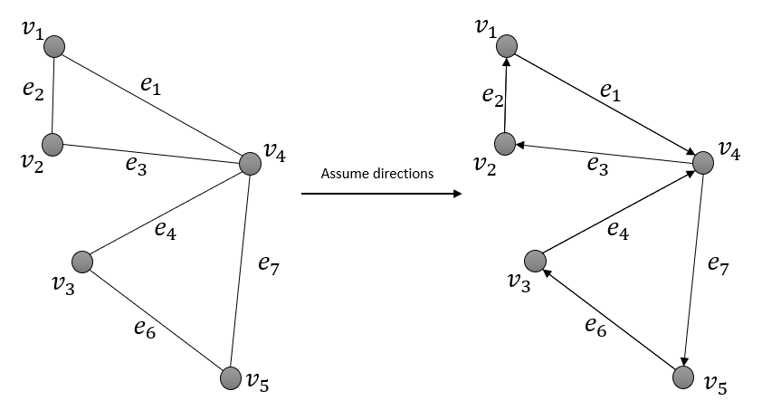
The mapping $f\longrightarrow\nabla f$ is known as the co-boundary mapping of the graph, we take an example from the graph as shown in Figure 1, we arrange arbitrary directions to the edges as the figure in right shows. We have

Accordingly, $\nabla\left[\begin{matrix}f_{1}\\ f_{2}\\ f_{3}\\ f_{4}\\ f_{5}\\ \end{matrix}\right]=\left[\begin{matrix}-1&0&0&1&0\\ 1&-1&0&0&0\\ 0&1&0&-1&0\\ 0&0&-1&1&0\\ 0&0&0&-1&1\\ 0&0&1&0&-1\\ \end{matrix}\right]\left[\begin{matrix}f_{1}\\ f_{2}\\ f_{3}\\ f_{4}\\ f_{5}\\ \end{matrix}\right]=\left[\begin{matrix}f_{4}-f_{1}\\ f_{1}-f_{2}\\ f_{2}-f_{4}\\ f_{4}-f_{3}\\ f_{5}-f_{4}\\ f_{3}-f_{5}\\ \end{matrix}\right]$

Therefore, $(\nabla f)(e_{i,j})$ is given by

where $e_{i,j}$ denote the edge connecting node $i$ and node $j$.

Furthermore,

Thus, the Laplacian matrix $L$ operating on $g$ would become

Therefore, for any undirected graph,

Particularly, for an $n$-dimensional Euclidean space, the Laplacian operator can be considered as a second-order differential operator

Analogously, consider undirected weighted graphs $\mathcal{G}$, each edge $e_{i,j}$ is weighted by $w_{i,j}>0$, the Laplace operator on the graph can be defined as

where $W_{i,j}=0$ if $e_{i,j}\in\mathcal{E}$.

Also,

For any $i$ holds, then it can be general form:

As a quadratic form,

Therefore, graph Laplacian matrix $L$, intrinsically as a Laplacian operator, make the centre node subtracts the surrounding nodes in turn, multiplying the corresponding link weights at the same time, and then sums them.

In some cases of practical application, Laplacian matrix requires some kinds of normalization to ensure the algorithm convergence. Normalization of Laplacian matrix $\mathcal{L}$ include:

• •

  Random-walk normalization:

  $$\mathcal{L}=I-D^{-1}A$$

  (16)

• •

  Symmetric normalization:

  $$\mathcal{L}=D^{-1/2}LD^{-1/2}=I-D^{-1/2}WD^{-1/2},$$

  (17)

  with the convention $D^{-1}_{i,i}=0$ for $d_{i}=0$, particularly, node $i$ is an isolated vertex if $d_{i}=0$. A graph is said to be non-trivial if it contains at least one edge [9, Section 1.2]. The normalized Laplacian has eigenvalues always lying in the range between 0 and 2 inclusive as demonstrated by Chung [9, Section 1.3].

In the following, we will use symmetric normalized Laplacian matrix as default, unless unless otherwise stated.

The spectral GCN analysis relies on spectral graph theory, which studies the properties of graphs via the eigenvalues and its corresponding eigenvectors associated with the graph adjacency matrix and the graph Laplacian matrix and its variants. Since graph convolutional operator is defined on eigenvalues of the Laplacian matrix, being familiar with the properties of graph-related properties (as the facts listed below) is greatly helpful for the research on spectral GCN.

The eigenvalues of the Laplacian matrix can be inferred from the properties of the graph, for example:

Theorem 3.1 gives us the range of the eigenvalues of the normalized Laplacian matrix $\mathcal{L}$. For a stable graph filter of GCNs, it requires the absolute eigenvalues of $\mathcal{L}$ to be bounded by 1, thus various scaling methods are introduced as follows.

The principal of convolutional neural network is beyond the discussion of this paper, we refer the readers to [32] for a fundamental understanding. In the following, we will define graph filter, which is an convolution operator on graph in the fourier domain, as well as other associated concepts, which leads to various classic GCN models.

In the Fourier domain, the convolution operator on graph $\cdot_{G}$ is defined as

where $(\cdot_{G})$ is convolution operator defined on graph, $\odot$ is Hadamard product.

It follows that a signal $f$ is filtered by $g\in\mathbb{R}^{n}$, and denotes $g_{\theta}(\Lambda)=diag(U^{T}g)$ which the diagonal corresponds to spectral filter coefficients.

For details,

Spectral-based GCN all follow this definition of $Ug_{\theta}(\Lambda)U^{T}f$, the main difference between different version of Spectral-based GCN lies in the choice of the filter $g_{\theta}(\Lambda)$ [58].

Bruna et al. propose the first spectral convolutional neural network [5]. A graph can be associated with node signal $f\in\mathbb{R}^{n\times C_{k}}$ is a feature matrix with $f_{i}\in\mathbb{R}^{C_{k}}$ representing the feature vector of node $i$. A construction where each layer $k=1,\ldots,K$ transforms an input vector $f^{(k)}$ of size $n\times C_{k}$ into an output $f^{(k+1)}$ of size $n\times C_{k+1}$.

where ${g_{\theta}}_{i,j}^{(k)},i=1,\ldots,n;j=1,\ldots,C_{k}$ is a diagonal matrix with trainable parameters $\theta_{m}^{(k)},m\in(1,n)$, $\sigma$ is activation function. ${g_{\theta}}_{i,j}^{(k)}$ is given by

ChebNet [12] uses Chebyshev polynomials instead of convolutions in spectral domain. Furthermore, it was demonstrated that that $g_{\theta}(\Lambda)$ can be approximated by a truncated expansion in terms of Chebyshev polynomials [22].

where $T_{0}(x)=1,T_{1}=x$. Here, we make $\widetilde{\Lambda}=\frac{2\Lambda}{\lambda_{max}}-I_{n}\in[-1,1]$, $\lambda_{max}$ is the biggest eigenvalue from $\mathcal{L}$

where the parameter $\theta\in\mathbb{R}^{K}$.

The filtering operator can also be written as

where $T_{k}(\tilde{\mathcal{L}})\in\mathbb{R}^{n\times n}$ is the Chebyshev polinomial of order $k$ evaluated at the scaled Laplacian $\tilde{\mathcal{L}}=2\mathcal{L}/\lambda_{max}-I_{n}$. Accordingly, spectral filters represented by $K^{th}$-order polynomials of the Laplacian are exactly $K$-localized, i.e. it depends only on nodes that are at maximum $K$ steps away from the central node [12], [22, Lemma 5.2].

The Lemma can be used to demonstrate that matrix elements of low powers of the graph Laplacian corresponding to sufficiently separated vertices must be zero. Therefore, $dist(v_{i},v_{j})>K$ implies $(\mathcal{L}^{K})_{i,j}=0$, and the spectral filters of ChebNet are exactly $K$-localized.

Accordingly,

where $\theta_{k}$ is a vector of Chebyshev coefficients, which is trainable parameter.

Furthermore, Equation 29 can be deduced as following

After using Chebyshev polynomial instead of the convolution kernel of the spectral domain, ChebNet does not need the Laplace matrix is to be eigen-decomposed. The most time-consuming steps are omitted [12].

Comparison between Spectral CNN and ChebNet

Assuming that $n$ is the number of nodes.

• •

  The parameter complexity of the SCNN model is very large, and the learning complexity is $O(n)$ [5], [12, Section 2.1], which is easy to overfit when there are many nodes. When dealing with large-scale graph data which usually has more than millions of nodes, it will face great challenges.

• •

  Computing the eigenvalue decomposition of the Laplace matrix is very time-consuming.

• •

  The convolution kernel of ChebNet has only K learnable parameters($\theta_{k}$), and $K\ll n$, hence their learning complexity is $O(K)$, the complexity of learnable parameters is greatly reduced [12, Section 2.1].

• •

  ChebNet does not need the Laplace matrix to be eigen-decomposed, instead it approximate $g_{\theta}(\mathcal{L})$ with a truncated expansion in term of Chebyshev polynomials $T_{k}(x)$ of $K^{th}$ order [12, Section 2.1].

The paper [37] construct a family of complex filters that enjoy the advantages of Chebyshev filters while avoiding some of their drawbacks. A Cayley polynomial of order $r$ to be a real-valued function with complex coefficients.

where $c=(c_{0,\ldots,c_{r}})$ is a vector of one real coefficient and $r$ complex coefficients and $h>0$ is the spectral zoom parameter.

A Cayley filter $G$ is a spectral filter defined on real signals $f$ by

the parameters c and h is learnable, which are optimized during training.

The application of the filter $g_{\theta}(\mathcal{L})f$ can be performed without explicit expensive eigendecomposition of the Laplacian operator. The unit complex circle is denoted by $e^{i\mathbb{R}}=\{e^{i\theta},\theta\in\mathbb{R}\}$.

The Cayley transform $C(x)=\frac{x-i}{x+i}$ is a smooth bijection between $\mathbb{R}$ and $e^{i\mathbb{R}}\setminus\{1\}$.

Correspondingly, by applying the Cayley transform to the scaled Laplacian $h\mathcal{L}$, we get the complex matrix

which has its spectrum in $e^{i\mathbb{R}}$ and is thus unitary.

Since $z^{-1}=\overline{z}$ for $z\in e^{i\mathbb{R}}$, we have $\overline{c_{j}C^{j}(h\mathcal{L})}=\overline{c_{j}}C^{-j}(h\mathcal{L})$ and given $2Re{z}=z+\overline{z}$, any Cayley filter can be written as a conjugate-even Laurent polynomial.

proof:

Since the spectrum of $C(h\Delta)$ is in $e^{i\mathbb{R}}$, the operator $C^{j}(h\Delta)$ can be thought of as a multiplication by a pure harmonic in the frequency domain $e^{i\mathbb{R}}$ for any integer power $j$,

where $C^{j}(h\mathcal{L})$ it is a (real-valued) trigonometric polynomial, and $g_{\theta}(\Lambda)$ is conjugate-even.

Hence, a Cayley filter $g_{\theta}$ can be seen as a multiplication by a finite Fourier expansion in the frequency domain $e^{i\mathbb{R}}$. While preserving spatial locality, ChebNet can be considered as a special case of CayleyNet [37], [58].

GCN [29] can be regarded as a further simplification of ChebNet. To reduce the computational complexity, only the first order Chebyshev polynomials are considered, consequently each convolution kernel has only one trainable parameter [29]. Combining with (27), we have

Hence,

In this linear formulation of a GCN we further approximate $\lambda_{max}\approx 2$. Under such approximations, this can simplifies to:

where $\mathcal{L}$ is normalized graph Laplacian $\mathcal{L}=I-D^{-\frac{1}{2}}AD^{-\frac{1}{2}}$.

Then,

where $A$ is an adjacency matrix of the graph.

Accordingly,

Furthermore, to reduce the number of trainable parameters——each kernel has only one trainable parameter, we set $\theta_{0}=-\theta_{1}=\theta$, then we have

where $D^{-\frac{1}{2}}AD^{-\frac{1}{2}}+I_{n}$ now has eigenvalues in the range [0, 2]. Then, only one parameter in convolution kernel can be learned. The number of parameters is greatly reduced, which can reduce the number of parameters to prevent overfitting.

However, repeated application of this operator can therefore lead to numerical instabilities and exploding or vanishing gradients. To alleviate this problem, the following re-normalization trick is introduced.

We add self-loop to $A$,

Correspondingly,

Finally,

Usually, we write $\theta$ as $W,\hat{A}=\widetilde{D}^{-\frac{1}{2}}\widetilde{A}\widetilde{D}^{-\frac{1}{2}}$, then we have $f(\cdot_{G})g=\hat{A}fW$.

Here make an illustration of example(applied on Cora dataset, a node level task), consider a two-layer GCN for semi-supervised node classification on a graph, $f\in\mathbb{R}^{n\times C}$ is $n$ nodes with $C$ input channels

$W^{<0>}\in\mathbb{R}^{C\times H}$ is an input-to-hidden weight matrix for a hidden layer with H feature maps. $W^{<1>}\in\mathbb{R}^{H\times F}$ is a hidden-to-output weight matrix, $F$ is the dimension of feature maps in the output layer.

For calculation of loss function, need to evaluate the cross-entropy error over all labeled examples

References

- [1] H. Amini and M. Lelarge. The diameter of weighted random graphs. The Annals of Applied Probability, 25, 2011.
- [2] D. Beck, G. Haffari, and T. Cohn. Graph-to-sequence learning using gated graph neural networks. In Proceedings of the 56th Annual Meeting of the Association for Computational Linguistics (Volume 1: Long Papers), pages 273–283. Association for Computational Linguistics, 2018.
- [3] G. Berlusconi, F. Calderoni, N. Parolini, M. Verani, and C. Piccardi. Link prediction in criminal networks: A tool for criminal intelligence analysis. PLOS ONE, 11(4):1–21, 04 2016.
- [4] M. Bronstein, J. Bruna, Y. Lecun, A. Szlam, and P. Vandergheynst. Geometric deep learning: Going beyond euclidean data. IEEE Signal Processing Magazine, 34(4):18–42, 2017.
- [5] J. Bruna, W. Zaremba, A. Szlam, and Y. Lecun. Spectral networks and locally connected networks on graphs. In International Conference on Learning Representations, 2014.
- [6] S. Butler. Eigenvalues and structures of graphs. PhD thesis, UC San Diego, 2008.
- [7] S. Butler and F. Chung. Spectral Graph Theory. CBMS, ANS, 2013.
- [8] S. Chen, R. Varma, A. Sandryhaila, and J. Kovačević. Discrete signal processing on graphs: Sampling theory. IEEE Transactions on Signal Processing, 63(24):6510–6523, 2015.
- [9] F. R. K. Chung. Spectral Graph Theory. American Mathematical Society, 1997.
- [10] Z. Cui, K. Henrickson, R. Ke, and Y. Wang. Traffic graph convolutional recurrent neural network: A deep learning framework for network-scale traffic learning and forecasting. IEEE Transactions on Intelligent Transportation Systems, PP, 2019.
- [11] H. Dai, Z. Kozareva, B. Dai, J. A. Smola, and L. Song. Learning steady-states of iterative algorithms over graphs. ICML, pages 1114–1122, 2018.
- [12] M. Defferrard, X. Bresson, and P. Vandergheynst. Convolutional neural networks on graphs with fast localized spectral filtering. In Proceedings of the 30th International Conference on Neural Information Processing Systems, NIPS’16, pages 3844––3852. Curran Associates Inc., 2016.
- [13] C. Farabet, C. Couprie, L. Najman, and Y. LeCun. Learning hierarchical features for scene labeling. IEEE Transactions on Pattern Analysis and Machine Intelligence, 35(8):1915–1929, 2013.
- [14] E. Gallopoulos and Y. Saad. Efficient solution of parabolic equations by krylov approximation methods. SIAM Journal on Scientific and Statistical Computing, 13(5):1236–1264, 1992.
- [15] T. Glasmachers. Limits of end-to-end learning. In ACML, 2017.
- [16] G. H. Golub and C. F. Van Loan. Matrix Computations. The Johns Hopkins University Press, third edition, 1996.
- [17] M. Gori, G. Monfardini, and F. Scarselli. A new model for learning in graph domains. In Proceedings of IEEE International Joint Conference on Neural Networks, 2005., volume 2, pages 729–734. IEEE, 2005.
- [18] A. Greenbaum. Iterative Methods for Solving Linear Systems. Society for Industrial and Applied Mathematics, 1997.
- [19] S. Güttel. Rational krylov approximation of matrix functions: Numerical methods and optimal pole selection. GAMM Mitteilungen, 36, 2013.
- [20] W. H. Haemers. Interlacing eigenvalues and graphs. Linear Algebra and its Applications, 1995.
- [21] W. L. Hamilton. Graph representation learning. Synthesis Lectures on Artificial Intelligence and Machine Learning, 14(3):1–159, 2020.
- [22] D. K. Hammond, P. Vandergheynst, and R. Gribonval. Wavelets on graphs via spectral graph theory. Applied and Computational Harmonic Analysis, 30(2):129–150, 2011.
- [23] K. He, X. Zhang, S. Ren, and J. Sun. Deep residual learning for image recognition. In IEEE Conference on Computer Vision and Pattern Recognition, pages 770–778. IEEE, 2016.
- [24] G. Hinton, L. Deng, D. Yu, G. E. Dahl, A. Mohamed, N. Jaitly, A. Senior, V. Vanhoucke, P. Nguyen, T. N. Sainath, and B. Kingsbury. Deep neural networks for acoustic modeling in speech recognition: The shared views of four research groups. IEEE Signal Processing Magazine, 29(6):82–97, 2012.
- [25] J. Hua, Z. Zhong, and J. Hu. Spectral Geometry of Shapes: Principles and Applications. Computer Vision and Pattern Recognition. Elsevier Science, 2019.
- [26] K. Jha, S. Saha, and H. Singh. Prediction of protein–protein interaction using graph neural networks. Scientific Reports, 12(1):8360, 2022.
- [27] D. Jiang, Z. Wu, C.-Y. Hsieh, G. Chen, B. Liao, Z. Wang, C. Shen, D. Cao, J. Wu, and T. Hou. Could graph neural networks learn better molecular representation for drug discovery? a comparison study of descriptor-based and graph-based models. Journal of Cheminformatics, 13(1):12, 2021.
- [28] Y. Kim. Convolutional neural networks for sentence classification. In Proceedings of the Conference on Empirical Methods in Natural Language Processing), pages 1746–1751. Association for Computational Linguistics, 2014.
- [29] T. N. Kipf and M. Welling. Semi-Supervised Classification with Graph Convolutional Networks. In Proceedings of the 5th International Conference on Learning Representations, ICLR ’17, 2017.
- [30] A. Krizhevsky, I. Sutskever, and G. E. Hinton. Imagenet classification with deep convolutional neural networks. In F. Pereira, C. J. C. Burges, L. Bottou, and K. Q. Weinberger, editors, Advances in Neural Information Processing Systems 25, pages 1097–1105. Curran Associates, Inc., 2012.
- [31] D. Lazer, A. Pentland, L. Adamic, S. Aral, A.-L. Barabási, D. Brewer, N. Christakis, N. Contractor, J. Fowler, M. Gutmann, T. Jebara, G. King, M. Macy, D. Roy, and M. Van Alstyne. Computational social science. Science, 323(5915):721–723, 2009.
- [32] Y. LeCun, Y. Bengio, and G. Hinton. Deep learning. Nature, 521:436–444, 2015.
- [33] Y. LeCun, B. Boser, J. S. Denker, D. Henderson, R. E. Howard, W. Hubbard, and L. D. Jackel. Backpropagation applied to handwritten zip code recognition. Neural Computation, 1(4):541–551, 1989.
- [34] Y. LeCun, B. Boser, J. S. Denker, D. Henderson, R. E. Howard, W. Hubbard, and L. D. Jackel. Backpropagation applied to handwritten zip code recognition. Neural Computation, 1(4):541–551, 1989.
- [35] Y. Lecun, L. Bottou, Y. Bengio, and P. Haffner. Gradient-based learning applied to document recognition. Proceedings of the IEEE, 86(11):2278–2324, 1998.
- [36] Y. LeCun, K. Kavukcuoglu, and C. Farabet. Convolutional networks and applications in vision. In Proceedings of IEEE International Symposium on Circuits and Systems, pages 253–256. IEEE, 2010.
- [37] R. Levie, F. Monti, X. Bresson, and M. Bronstein. Cayleynets: Graph convolutional neural networks with complex rational spectral filters. Transactions on Signal Processing, 2017.
- [38] Y. Li, D. Tarlow, M. Brockschmidt, and R. S. Zemel. Gated graph sequence neural networks. In 4th International Conference on Learning Representations, ICLR 2016, San Juan, Puerto Rico, May 2-4, 2016, Conference Track Proceedings, 2016.
- [39] G. Lv, Z. Hu, Y. Bi, and S. Zhang. Learning unknown from correlations: Graph neural network for inter-novel-protein interaction prediction. In Proceedings of the 13th International Joint Conference on Artificial Intelligence, pages 3677–3683. International Joint Conferences on Artificial Intelligence Organization, 8 2021.
- [40] X. Ma, J. Wu, S. Xue, J. Yang, C. Zhou, Q. Z. Sheng, H. Xiong, and L. Akoglu. A comprehensive survey on graph anomaly detection with deep learning. IEEE Transactions on Knowledge and Data Engineering, pages 1–1, 2021.
- [41] X. Ma, J. Wu, J. Yang, and Q. Z. Sheng. Towards graph-level anomaly detection via deep evolutionary mapping. In Proceedings of the 29th SIGKDD Conference on Knowledge Discovery and Data Mining, KDD ’23, pages 1631–1642. ACM, 2023.
- [42] Y. Ma and J. Tang. Deep Learning on Graphs. Cambridge University Press, 2021.
- [43] D. Nathani, J. Chauhan, C. Sharma, and M. Kaul. Learning attention-based embeddings for relation prediction in knowledge graphs. In Proceedings of the 57th Annual Meeting of the Association for Computational Linguistics, pages 4710–4723. Association for Computational Linguistics, 2019.
- [44] G. Phillips. Interpolation and Approximation by Polynomials. Springer, 2003.
- [45] S. Ren, K. He, R. Girshick, and J. Sun. Faster R-CNN: Towards real-time object detection with region proposal networks. In C. Cortes, N. Lawrence, D. Lee, M. Sugiyama, and R. Garnett, editors, Advances in Neural Information Processing Systems, volume 28. Curran Associates, Inc., 2015.
- [46] A. Sandryhaila and J. M. F. Moura. Discrete signal processing on graphs. Transactions on Signal Processing, 61(7):1644–1656, 2013.
- [47] A. Sandryhaila and J. M. F. Moura. Discrete signal processing on graphs: Graph fourier transform. In IEEE International Conference on Acoustics, Speech and Signal Processing, pages 6167–6170. IEEE, 2013.
- [48] A. Sandryhaila and J. M. F. Moura. Discrete signal processing on graphs: Frequency analysis. IEEE Transactions on Signal Processing, 62(12):3042–3054, 2014.
- [49] F. Scarselli, M. Gori, A. C. Tsoi, M. Hagenbuchner, and G. Monfardini. The graph neural network model. IEEE Transactions on Neural Networks, 20(1):61–80, 2009.
- [50] Y. Seo, M. Defferrard, P. Vandergheynst, and X. Bresson. Structured sequence modeling with graph convolutional recurrent networks. ArXiv, abs/1612.07659, 2016.
- [51] D. I. Shuman, S. K. Narang, P. Frossard, A. Ortega, and P. Vandergheynst. The emerging field of signal processing on graphs: Extending high-dimensional data analysis to networks and other irregular domains. IEEE Signal Processing Magazine, 30:83–98, 2013.
- [52] D. Silver, A. Huang, C. Maddison, A. Guez, L. Sifre, G. Driessche, J. Schrittwieser, I. Antonoglou, V. Panneershelvam, M. Lanctot, S. Dieleman, D. Grewe, J. Nham, N. Kalchbrenner, I. Sutskever, T. Lillicrap, M. Leach, K. Kavukcuoglu, T. Graepel, and D. Hassabis. Mastering the game of Go with deep neural networks and tree search. Nature, 529:484–489, 2016.
- [53] A. Susnjara, N. Perraudin, D. Kressner, and P. Vandergheynst. Accelerated filtering on graphs using lanczos method. arXiv, pages 1–11, 2015.
- [54] A. van den Oord, S. Dieleman, H. Zen, K. Simonyan, O. Vinyals, A. Graves, N. Kalchbrenner, A. W. Senior, and K. Kavukcuoglu. Wavenet: A generative model for raw audio. In The 9th ISCA Speech Synthesis Workshop, Sunnyvale, CA, USA, 13-15 September 2016, page 125. ISCA, 2016.
- [55] P. Velickovic, G. Cucurull, A. Casanova, A. Romero, P. Liò, and Y. Bengio. Graph attention networks. ArXiv, abs/1710.10903, 2018.
- [56] D. E. Worrall, S. J. Garbin, D. Turmukhambetov, and G. J. Brostow. Harmonic networks: Deep translation and rotation equivariance. arXiv, abs/1612.04642, 2016.
- [57] L. Wu, P. Cui, J. Pei, and L. Zhao. Graph Neural Networks: Foundations, Frontiers, and Applications. Springer, Singapore, 2022.
- [58] Z. Wu, S. Pan, F. Chen, G. Long, C. Zhang, and P. S. Yu. A comprehensive survey on graph neural networks. IEEE Transactions on Neural Networks and Learning Systems, 32:4–24, 2021.
- [59] G. Zhang, Z. Yang, J. Wu, J. Yang, S. Xue, H. Peng, J. Su, C. Zhou, Q. Z. Sheng, L. Akoglu, and C. C. Aggarwal. Dual-discriminative graph neural network for imbalanced graph-level anomaly detection. In Advances in Neural Information Processing Systems, 2022.
- [60] Q. Zhang, X. Wang, Y. Wu, H. Zhou, and S. Zhu. Interpretable CNNs for object classification. IEEE Transactions on Pattern Analysis and Machine Intelligence, 43(10):3416–3431, 2021.
- [61] R. Zhang. Making convolutional networks shift-invariant again. arXiv, abs/1904.11486, 2019.
- [62] X.-M. Zhang, L. Liang, L. Liu, and M.-J. Tang. Graph neural networks and their current applications in bioinformatics. Frontiers in Genetics, 12, 2021.
- [63] Z. Zhang, P. Cui, and W. Zhu. Deep learning on graphs: A survey. ArXiv, abs/1812.04202, 2018.
- [64] J. Zhou, G. Cui, S. Hu, Z. Zhang, C. Yang, Z. Liu, L. Wang, C. Li, and M. Sun. Graph neural networks: A review of methods and applications. AI Open, 1:57–81, 2020.