跳到论文正文
W Papers独立论文阅读器 arXiv:2012.06648 论文正文 计算阅读时间 · 0%
引用这篇论文根据当前论文元数据生成,正式投稿前建议核对。


License: arXiv.org perpetual non-exclusive license
arXiv:2012.06648v2 [math.PR] 04 Aug 2021

Large Deviations of Cancer Recurrence Timing

Pranav Hanagal    Kevin Leder    Zicheng Wang
Abstract

We study large deviation events in the timing of disease recurrence. In particular, we are interested in modeling cancer treatment failure due to mutation induced drug resistance. We first present a two-type branching process model of this phenomenon, where an initial population of cells that are sensitive to therapy can produce mutants that are resistant to the therapy. In this model we investigate two random times, the recurrence time and the crossover time. Recurrence time is defined as the first time that the population size of mutant cells exceeds a given proportion of the initial population size of drug-sensitive cells. Crossover time is defined as the first time that the resistant cell population dominates the total population. We establish convergence in probability results for both recurrence and crossover time. We then develop expressions for the large deviations rate of early recurrence and early crossover events. We characterize how the large deviation rates and rate functions depend on the initial size of the mutant cell population. We finally look at the large deviations rate of early recurrence conditioned on the number of mutant clones present at recurrence in the special case of deterministically decaying sensitive population. We find that if recurrence occurs before the predicted law of large numbers limit then there will likely be an increase in the number of clones present at recurrence time.
Keywords: Cancer evolution; Large deviation principle; Branching processes.

1 Introduction

In the past two decades, targeted therapies have been developed and applied to treat many types of cancers (chronic myeloid leukemia, non-small cell lung cancer, etc). Many of these therapies lead to a substantial decline in tumor burden. However, mutation-induced drug resistance often occurs and results in cancer recurrence. Therefore, it is of particular importance to understand the evolutionary dynamics of cancer recurrence. Currently, little is known about the scenarios where cancers recur abnormally earlier than expected. In this work, we develop a stylized model to analyze these rare events and provide information on the number of clones of mutants conditioned on early recurrence.

Mathematical modeling can help in the understanding of complicated cellular dynamics. A large number of mathematical models have been proposed and analyzed to study the dynamics of bacterial and cancer cell populations and the evolution of drug resistance. Luria and Delbrück [13] built a simple model (LD model) in which sensitive and resistant bacteria grow deterministically, while mutation occurs randomly. They derived the distribution of the number of resistant bacteria, and formulated a function to estimate the mutation rate. Iwasa, Nowak and Michor [8] analyzed a stochastic LD model (with some deterministic approximations) and obtained the probability of resistance, the mean number of mutants, and the distribution of the number of mutants when the cell population reached a detection size. Kessler and Levine [12] studied the fully stochastic LD model and derived the probability distribution for the number of mutants when the cell population reached a large size (large population size limit). Keller and Antal [11] studied the LD model with stochastic growth of the resistant population. They obtained an exact formula for the generating function of the number of mutants when the number of drug-sensitive cells reach a given threshold. Cheek and Antal [3] investigated the fully stochastic LD model and obtained valuable results for the “mutation times, clone sizes and number of mutants” in different settings. All of these works provide valuable insights into how mutations accumulate during tumor expansion (prior to treatment), while our work focuses on what happens during treatment.

Our work is based on a stream of literature studying multi-type branching processes. Durrett [4] summarized a lot of important results concerning two stochastic times: the time of the first type k mutation, and the time of the first type k mutation that founds a family line that does not go extinct. Such results can be applied to cancer treatment, such as finding a “window of opportunity for screening.” Jagers and co-authors [9, 10] obtained results for the “path to extinction” in subcritical branching processes, including convergence of finite dimensional distributions and its extension to general inter-arrival times. In this work, we will utilize the same time scale as considered in [9, 10]. Foo and Leder [5] used a branching process model to analyze the dynamics of escape from extinction. They studied the time at which the total cell population begins to rebound (the population stops declining and starts increasing) as well as the crossover time (the first time at which the total cell population is dominated by the mutant cell population). Foo, Leder and Zhu [6] extended the study of escape times to include random mutational fitness advantage, which means that each mutation results in the creation of a supercritical birth-death process with random birth rate. The authors further established a functional central limit theorem for a scaled version of the mutant cell process. Lastly Antal and Avanzini [2] investigated time to disease recurrence due to possibly occult metastasis in a branching process model of cancer.

In this work we develop a number of results concerning the recurrence and crossover times. We examine the dynamics between drug-sensitive cells and mutant cells during treatment. We also incorporate the initial size of mutant population prior to treatment which haven’t been studied in [5] and [6]. Clinical studies have shown that drug resistant mutations can be present prior to treatment [15], and it is therefore important to incorporate the initial size of mutant population.We focus on the particular rare event of early recurrence such that recurrence happens yy units of time earlier than the deterministic limit. We formulate the prediction of recurrence time in Section 2, and establish a convergence in probability result in Theorem 1. In Theorem 2, we obtain the large deviations rates and rate functions of early recurrence with respect to different sizes of initial mutant population. In particular, we examine three possible cases: (1) resistance is driven by mutants created during treatment, (2) resistance is driven by both pre-existing and acquired mutants, and (3) resistance is driven by pre-existing mutants. We observe that in case (1) and (2), rate functions depend on the mutation parameter μ\mu, while it doesn’t in case (3). Moreover, in all three cases, the decay rate increases in yy. In Section 3.1, the large deviations results have also been established for the crossover time. We find that the large deviations rates are similar for the two random times, but the large deviations rate for crossover time is more sensitive to the decay rate of the sensitive cell population. In Section 3.2, we study the rare event of early recurrence conditioned on a fixed number of mutant clones at yy units of time before the deterministic limit. We then use this result to find the number of clones which minimizes the decay rate, i.e., the number of clones that is most likely to lead to an early recurrence. We observe that this optimal number of clones increases in yy, which indicates that early recurrence leads to a larger number of mutant clones present at recurrence.

The remainder of this work is organized as follows. In Section 2, we describe our model and present important results from previous works. In Section 3, we state the main results and their implications. In Section 4, we provide proofs of our main results.

2 Model and Previous Results

In this section, we introduce the multi-type branching process model, as well as the recurrence time and crossover time. Our model is similar to the models studied in [5] and [6].

Consider a subcritical birth-death process (Z0n​(t))t≥0\left(Z_{0}^{n}\left(t\right)\right)_{t\geq 0} with birth rate r0r_{0}, death rate d0d_{0} and net growth rate λ0=r0−d0<0\lambda_{0}=r_{0}-d_{0}<0. Z0nZ_{0}^{n} represents the drug-sensitive wild-type population with Z0n​(0)=nZ_{0}^{n}\left(0\right)=n. For our convenience, we will additionally define r=−λ0r=-\lambda_{0}. Consider a supercritical birth-death process (Z1n​(t))t≥0\left(Z_{1}^{n}\left(t\right)\right)_{t\geq 0} with birth rate r1r_{1}, death rate d1d_{1} and net growth rate λ1=r1−d1>0\lambda_{1}=r_{1}-d_{1}>0. Z1nZ_{1}^{n} represents the drug-resistant mutants that preexist treatment (type-11 mutants) with Z1n​(0)=X⁡(n)Z_{1}^{n}\left(0\right)=X\left(n\right). Drug-resistant mutants are also generated during treatment at time tt at rate Z0n​(t)​μ​n−αZ_{0}^{n}\left(t\right)\mu n^{-\alpha} for α∈(0,1)\alpha\in\left(0,1\right), and each of these mutations results in the creation of a clone which is modeled as a supercritical birth-death process with birth rate r1r_{1}, death rate d1d_{1} and net growth rate λ1=r1−d1>0\lambda_{1}=r_{1}-d_{1}>0. We denote this population (type-22 mutants) by (Z2n​(t))t≥0\left(Z_{2}^{n}\left(t\right)\right)_{t\geq 0}. Then Z2nZ_{2}^{n} is a supercritical branching process with immigration. To clarify the model, we note that mutants modeled by Z1nZ_{1}^{n} and Z2nZ_{2}^{n} behave exactly the same. They are only different in terms of their ancestors. For each n≥1n\geq 1, the processes (Z0n,Z1n,Z2n)(Z_{0}^{n},Z_{1}^{n},Z_{2}^{n}) are defined on a common probability space (Ωn,ℱn,ℙn)(\Omega_{n},\mathcal{F}^{n},\mathbb{P}_{n}). For ease of notation we will write ℙ\mathbb{P} instead of ℙn\mathbb{P}_{n}.

To simplify notation, we define for i=0,1,2i=0,1,2 the functions

zin​(t)=𝔼​Zin​(t).z_{i}^{n}\left(t\right)=\mathbb{E}Z_{i}^{n}\left(t\right).

If we use the time scale tn=1r​log​(n)t_{n}=\frac{1}{r}\text{log}\left(n\right), then the following results are known from [5], [6], and [1]:

z0n​(u​tn)=n​e−r​u​tn=n1−u,\displaystyle z_{0}^{n}\left(ut_{n}\right)=ne^{-rut_{n}}=n^{1-u},
z1n​(u​tn)=X⁡(n)​eλ1​u​tn=X⁡(n)​nλ1r​u,\displaystyle z_{1}^{n}\left(ut_{n}\right)=X\left(n\right)e^{\lambda_{1}ut_{n}}=X\left(n\right)n^{\frac{\lambda_{1}}{r}u},
z2n​(u​tn)=μλ1+r​n1−α​eλ1​u​tn​(1−e(λ0−λ1)​u​tn)=μλ1+r​n1−α​(nλ1r​u−n−u),\displaystyle z_{2}^{n}\left(ut_{n}\right)=\frac{\mu}{\lambda_{1}+r}n^{1-\alpha}e^{\lambda_{1}ut_{n}}\left(1-e^{\left(\lambda_{0}-\lambda_{1}\right)ut_{n}}\right)=\frac{\mu}{\lambda_{1}+r}n^{1-\alpha}\left(n^{\frac{\lambda_{1}}{r}u}-n^{-u}\right),
Var⁡(Z0n​(u​tn))=r0+d0r​n1−u​(1−n−u),\displaystyle{\rm Var}\left(Z_{0}^{n}\left(ut_{n}\right)\right)=\frac{r_{0}+d_{0}}{r}n^{1-u}\left(1-n^{-u}\right),
Var⁡(Z1n​(u​tn))=X⁡(n)​r1+d1λ1​nλ1r​u​(nλ1r​u−1).\displaystyle{\rm Var}\left(Z_{1}^{n}\left(ut_{n}\right)\right)=X\left(n\right)\frac{r_{1}+d_{1}}{\lambda_{1}}n^{\frac{\lambda_{1}}{r}u}\left(n^{\frac{\lambda_{1}}{r}u}-1\right).

We also define the moment generating function of a binary branching process starting from a single cell. Let Z={Z⁡(t),t≥0}Z=\{Z\left(t\right),t\geq 0\} denote a binary branching process where Z⁡(0)=1Z\left(0\right)=1 and each individual cell has birth rate r1r_{1}, death rate d1d_{1}, and net growth rate λ1=r1−d1\lambda_{1}=r_{1}-d_{1}. The moment generating function is given by

ϕt​(θ)=𝔼​exp⁡(θ​Z​(t))={d1​(eθ−1)−e−λ1​t​(r1​eθ−d1)r1​(eθ−1)−e−λ1​t​(r1​eθ−d1),θ<θ¯t∞θ≥θ¯t\displaystyle\phi_{t}\left(\theta\right)=\mathbb{E}\exp\left(\theta Z\left(t\right)\right)=\left\{\begin{array}[]{cc}\frac{d_{1}\left(e^{\theta}-1\right)-e^{-\lambda_{1}t}\left(r_{1}e^{\theta}-d_{1}\right)}{r_{1}\left(e^{\theta}-1\right)-e^{-\lambda_{1}t}\left(r_{1}e^{\theta}-d_{1}\right)},&\hskip 14.22636pt\theta<\bar{\theta}_{t}\\ \infty&\hskip 14.22636pt\theta\geq\bar{\theta}_{t}\\ \end{array}\right.

where

θ¯t≐log⁡(r1​eλ1​t−d1r1​eλ1​t−r1)\bar{\theta}_{t}\doteq\log\left(\frac{r_{1}e^{\lambda_{1}t}-d_{1}}{r_{1}e^{\lambda_{1}t}-r_{1}}\right) (2.3)

(see page 109 of [1]). Throughout this paper, we will repeatedly use ϕt\phi_{t} to denote the moment generating function of Z⁡(t)Z(t).

We are interested in the asymptotic properties of the recurrence time which we define as

γn​(a)=inf{t≥0:Z1n​(t)+Z2n​(t)>a​n}\gamma_{n}\left(a\right)=\inf\{t\geq 0:Z_{1}^{n}\left(t\right)+Z_{2}^{n}\left(t\right)>an\}

for a>0a>0. We will often be interested in γn​(1)\gamma_{n}(1), and use the notation γn≡γn​(1)\gamma_{n}\equiv\gamma_{n}(1). Recurrence time represents the first time that the mutant cell population given by Z1n​(t)+Z2n​(t)Z_{1}^{n}\left(t\right)+Z_{2}^{n}\left(t\right) exceeds a proportion aa of the initial population size of drug-sensitive cells. We denote by ζn​(a)\zeta_{n}\left(a\right) the unique solution to z1n​(t)+z2n​(t)=a​nz_{1}^{n}\left(t\right)+z_{2}^{n}\left(t\right)=an. We will show that γn​(a)−ζn​(a)→0\gamma_{n}\left(a\right)-\zeta_{n}\left(a\right)\rightarrow 0 in probability. Due to the complexity of the equation z1n​(t)+z2n​(t)=a​nz_{1}^{n}\left(t\right)+z_{2}^{n}\left(t\right)=an, we cannot get an explicit form of ζn​(a)\zeta_{n}\left(a\right). Instead we solve the equation (by noting that z2n​(t)≥μλ1+r​n1−α​eλ1​t​(1−e−λ1​t)z_{2}^{n}\left(t\right)\geq\frac{\mu}{\lambda_{1}+r}n^{1-\alpha}e^{\lambda_{1}t}\left(1-e^{-\lambda_{1}t}\right))

(X⁡(n)+μλ1+r​n1−α)​eλ1​t−μλ1+r​n1−α=a​n\left(X\left(n\right)+\frac{\mu}{\lambda_{1}+r}n^{1-\alpha}\right)e^{\lambda_{1}t}-\frac{\mu}{\lambda_{1}+r}n^{1-\alpha}=an (2.4)

to get an upper bound u¯nu​p​p​e​r=1λ1​log⁡(a​n+μλ1+r​n1−αX⁡(n)+μλ1+r​n1−α)\bar{u}_{n}^{upper}=\frac{1}{\lambda_{1}}\log\left(\frac{an+\frac{\mu}{\lambda_{1}+r}n^{1-\alpha}}{X\left(n\right)+\frac{\mu}{\lambda_{1}+r}n^{1-\alpha}}\right). Similarly we solve the equation (by noting that z2n​(t)≤μλ1+r​n1−α​eλ1​tz_{2}^{n}\left(t\right)\leq\frac{\mu}{\lambda_{1}+r}n^{1-\alpha}e^{\lambda_{1}t})

(X⁡(n)+μλ1+r​n1−α)​eλ1​t=a​n\left(X\left(n\right)+\frac{\mu}{\lambda_{1}+r}n^{1-\alpha}\right)e^{\lambda_{1}t}=an (2.5)

to get a lower bound u¯nl​o​w​e​r=1λ1​log⁡(a​nX⁡(n)+μλ1+r​n1−α)\bar{u}_{n}^{lower}=\frac{1}{\lambda_{1}}\log\left(\frac{an}{X\left(n\right)+\frac{\mu}{\lambda_{1}+r}n^{1-\alpha}}\right), which satisfies,

u¯nu​p​p​e​r−u¯nl​o​w​e​r=1λ1​log⁡(a​n+μλ1+r​n1−αa​n)→0, as ​n→∞.\displaystyle\bar{u}_{n}^{upper}-\bar{u}_{n}^{lower}=\frac{1}{\lambda_{1}}\log\left(\frac{an+\frac{\mu}{\lambda_{1}+r}n^{1-\alpha}}{an}\right)\rightarrow 0,\text{ as }n\rightarrow\infty.

With the convergence in probability result (Theorem 1), it is easy to notice that an ‘early recurrence’, which we denote by {γn(a)≤ζn(a)−y}\{\gamma_{n}\left(a\right)\leq\zeta_{n}\left(a\right)-y\}, is a rare event if we take nn sufficiently large. In this work, we will show that the probability of an early recurrence decays exponentially fast, and the corresponding rate and rate function depend on the initial number of mutant cells.

Foo, Leder and Zhu [6] study a different stochastic time for a closely related model. In particular define the crossover time as

τn=inf{t≥0:Z1n​(t)+Z2n​(t)>Z0n​(t)}.\tau_{n}=\inf\{t\geq 0:Z_{1}^{n}(t)+Z_{2}^{n}(t)>Z_{0}^{n}(t)\}.

In addition define ξn\xi_{n} as the unique solution to z1n​(t)+z2n​(t)=z0n​(t)z_{1}^{n}(t)+z_{2}^{n}(t)=z_{0}^{n}(t). In [6] they establish that ξn−τn→0\xi_{n}-\tau_{n}\to 0 as n→∞n\to\infty and establish a central limit theorem for fluctuations of τn\tau_{n} away from ξn\xi_{n}. In this work we focus on the recurrence time, but our main results have also been established for the crossover time and this can be found in Section 3.1.

Throughout this work we will use the following notation for the asymptotic behavior of positive functions:

f⁡(t)∼g⁡(t)\displaystyle f\left(t\right)\sim g\left(t\right) if f⁡(t)/g⁡(t)→1 as t→∞,\displaystyle\quad\hbox{if $f\left(t\right)/g\left(t\right)\to 1$ as $t\to\infty$},
f⁡(t)=o⁡(g⁡(t))\displaystyle f\left(t\right)=o\left(g\left(t\right)\right) if f⁡(t)/g⁡(t)→0 as t→∞,\displaystyle\quad\hbox{if $f\left(t\right)/g\left(t\right)\to 0$ as $t\to\infty$},
f⁡(t)=O⁡(g⁡(t))\displaystyle f\left(t\right)=O\left(g\left(t\right)\right) if f⁡(t)≤C​g​(t) for all t,\displaystyle\quad\hbox{if $f\left(t\right)\leq Cg\left(t\right)$ for all $t$},
f⁡(t)=Θ⁡(g⁡(t))\displaystyle f\left(t\right)=\Theta\left(g\left(t\right)\right) if c​g​(t)≤f⁡(t)≤C​g​(t) for all t,\displaystyle\quad\hbox{if $cg\left(t\right)\leq f\left(t\right)\leq Cg\left(t\right)$ for all $t$},

where CC and cc are positive constants.

3 Results

We first establish the convergence in probability result for the recurrence time.

Theorem 1

Assume that α∈(0,1)\alpha\in\left(0,1\right), a>0a>0, X⁡(n)<nX\left(n\right)<n, and X⁡(n)X\left(n\right) is non-decreasing in nn, then for every ϵ>0\epsilon>0 we have that

limn→∞ℙ⁡(|γn​(a)−ζn​(a)|>ϵ)=0.\lim\limits_{n\rightarrow\infty}\mathbb{P}\left(|\gamma_{n}\left(a\right)-\zeta_{n}\left(a\right)|>\epsilon\right)=0.

Proof: Section 4.1.

The proof of Theorem 1 is similar to Theorem 11 of [6] but it extends the result by incorporating the initial size of mutant population. Recurrence time (sometimes called relapse time in literature) is very important in cancer treatment. Theorem 1 shows that if we have enough information about the mutation rate and the initial size of mutant population to certain therapy, then we can have a good approximation of the recurrence time.

Next, we establish the large deviations results for the probability of an early recurrence. In short, a large deviation result can be thought as finding c≥0c\geq 0 and L⁡(y)L\left(y\right) such that

ℙ⁡(γn​(a)≤ζn​(a)−y)=exp⁡[−nc​(L⁡(y)+o⁡(1))],\displaystyle\mathbb{P}\left(\gamma_{n}\left(a\right)\leq\zeta_{n}\left(a\right)-y\right)=\exp\left[-n^{c}\left(L\left(y\right)+o(1)\right)\right],

where we call ncn^{c} the large deviation rate and L⁡(y)L\left(y\right) the rate function. We investigate three cases: (1) X⁡(n)=o⁡(n1−α)X\left(n\right)=o\left(n^{1-\alpha}\right), (2) X⁡(n)∼n1−αX\left(n\right)\sim n^{1-\alpha} and (3) X⁡(n)∼n1−βX\left(n\right)\sim n^{1-\beta}, where 0<β<α0<\beta<\alpha. Case (1) is the setting where there is an insignificant amount of mutants present at diagnosis and resistance is driven by mutants created during treatment. Case (3) is the setting where resistance is driven by pre-existing mutants, and Case (2) is the critical case where both pre-existing and acquired mutants drive resistance.

Theorem 2

Assume that α∈(0,1)\alpha\in\left(0,1\right).

(1) When X⁡(n)=o⁡(n1−α)X\left(n\right)=o\left(n^{1-\alpha}\right),

limn→∞1n1−αlogℙ(γn(a)≤ζn(a)−y)=−supθ∈(0,1)[λ1​μ​θ​ey​λ1r1​(λ1+r)−λ1​μ​θr1∫0∞e−r​seλ1​s−θds].\lim\limits_{n\rightarrow\infty}\frac{1}{n^{1-\alpha}}\log\mathbb{P}\left(\gamma_{n}\left(a\right)\leq\zeta_{n}\left(a\right)-y\right)=-\sup\limits_{\theta\in\left(0,1\right)}\left[\frac{\lambda_{1}\mu\theta e^{y\lambda_{1}}}{r_{1}\left(\lambda_{1}+r\right)}-\frac{\lambda_{1}\mu\theta}{r_{1}}\int_{0}^{\infty}\frac{e^{-rs}}{e^{\lambda_{1}s}-\theta}ds\right].

(2) When X⁡(n)∼n1−αX\left(n\right)\sim n^{1-\alpha},

limn→∞1n1−α​log⁡ℙ⁡(γn​(a)≤ζn​(a)−y)\displaystyle\quad\lim\limits_{n\rightarrow\infty}\frac{1}{n^{1-\alpha}}\log\mathbb{P}\left(\gamma_{n}\left(a\right)\leq\zeta_{n}\left(a\right)-y\right)
=−supθ∈(0,1)[λ1​θ​(μ+λ1+r)​eλ1​yr1​(λ1+r)−log(1−λ1r1θθ−1)−λ1​μ​θr1∫0∞e−r​seλ1​s−θds].\displaystyle=-\sup\limits_{\theta\in\left(0,1\right)}\left[\frac{\lambda_{1}\theta\left(\mu+\lambda_{1}+r\right)e^{\lambda_{1}y}}{r_{1}\left(\lambda_{1}+r\right)}-\log\left(1-\frac{\lambda_{1}}{r_{1}}\frac{\theta}{\theta-1}\right)-\frac{\lambda_{1}\mu\theta}{r_{1}}\int_{0}^{\infty}\frac{e^{-rs}}{e^{\lambda_{1}s}-\theta}ds\right].

(3) When X⁡(n)∼n1−βX\left(n\right)\sim n^{1-\beta}, where 0<β<α0<\beta<\alpha,

limn→∞1n1−βlogℙ(γn(a)≤ζn(a)−y)=−supθ∈(0,1)[λ1​θ​eλ1​yr1−log(1−λ1r1θθ−1)].\lim\limits_{n\rightarrow\infty}\frac{1}{n^{1-\beta}}\log\mathbb{P}\left(\gamma_{n}\left(a\right)\leq\zeta_{n}\left(a\right)-y\right)=-\sup\limits_{\theta\in\left(0,1\right)}\left[\frac{\lambda_{1}\theta e^{\lambda_{1}y}}{r_{1}}-\log\left(1-\frac{\lambda_{1}}{r_{1}}\frac{\theta}{\theta-1}\right)\right].

For case (3), we can show that the optimal value of θ\theta is r1+d1−λ12+4​r1​d1​e−λ1​y2​d1\frac{r_{1}+d_{1}-\sqrt{{\lambda_{1}}^{2}+4r_{1}d_{1}e^{-\lambda_{1}y}}}{2d_{1}}. Surprisingly, in all three cases, the rate functions do not depend on the value of aa. The main reason is that the recurrence time is of order log⁡(a​n)=log⁡(a)+log⁡(n)\log\left(an\right)=\log\left(a\right)+\log\left(n\right), and hence the value of aa is negligible.

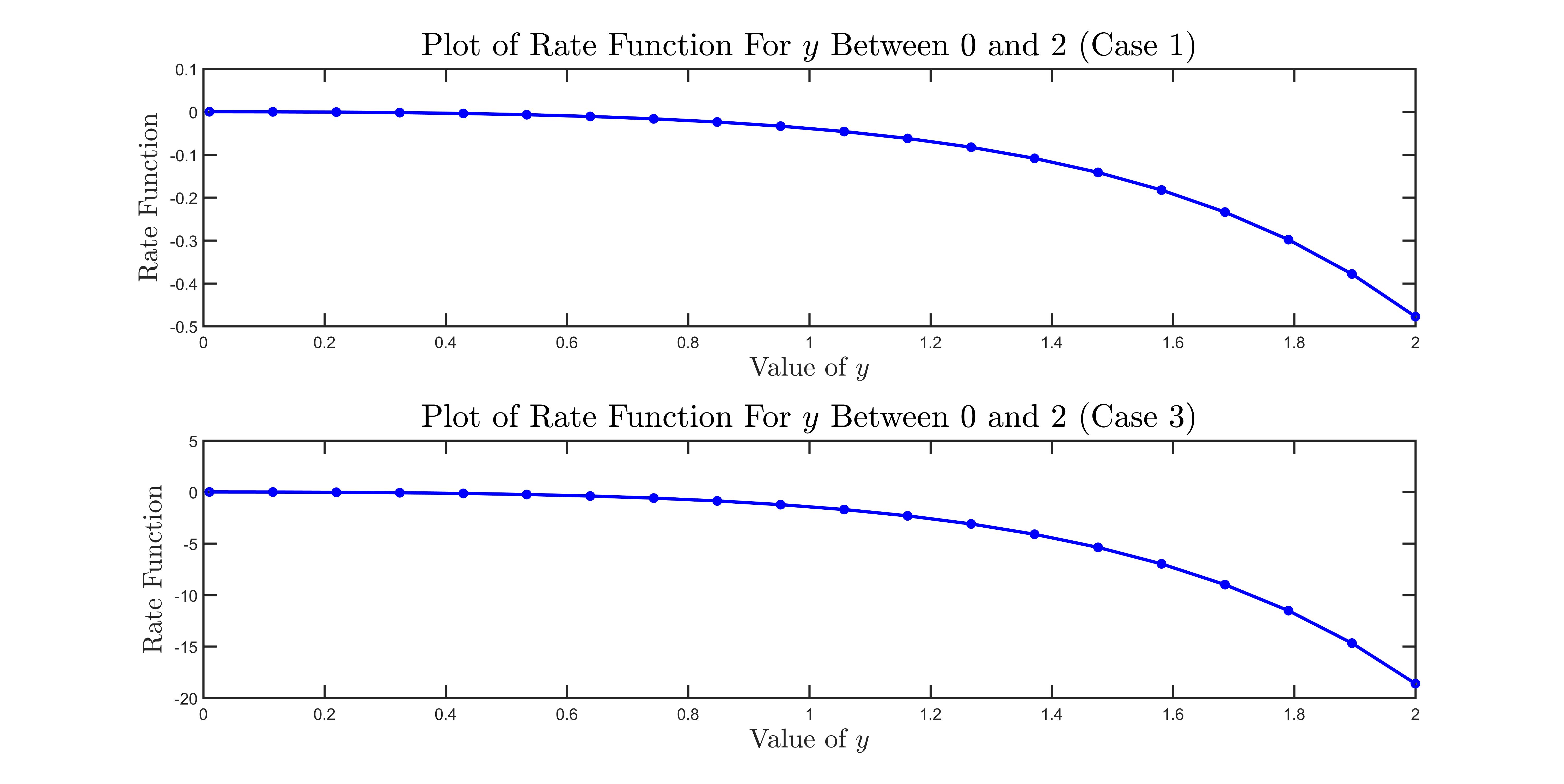
From Theorem 2 we can see that the large deviation rates and rate functions depend on the initial size of mutant cell population and the mutation rate. We can observe that the function within the supremum operator in Case (2) is the summation of those in Case (1) and Case (3), which is reasonable as Case (2) is the critical case. In all three cases, the rate function increases in yy which is intuitive as an earlier recurrence occurs with a lower probability. In Figure 1, we plot an example of the rate function for y∈(0,2)y\in\left(0,2\right) in Case (1) and Case (3).

We can also observe that in Case (1) and (2), the rate functions depend on μ\mu, while it doesn’t in Case (3). That is because mutation rate is irrelevant when resistance is driven by pre-existing mutants. Moreover, in Case (1), the rate function increases in μ\mu, which implies that when resistance is driven by mutants created during treatment, higher mutation rate leads to tighter concentration of recurrence time.

If we compare the decay rates (large deviation rate multiplied by rate function) of Case (1) and Case (3), we can observe that when nn is large, the decay rate of case (3) dominates (in magnitude) that of Case (1). The intuition is that the probability of early recurrence will have higher decay rate when more mutant cells accumulate early on. The reason is that a branching process will behave more deterministically when its initial size is larger. In Figure 2, we plot nβ−α​L1​(y)/L3​(y)n^{\beta-\alpha}L_{1}(y)/L_{3}(y) (which is the ratio of decay rates between Case (1) and Case (3)) for different values of β\beta, where L1L_{1} and L3L_{3} are the rate functions in Cases (1) and (3). Note that recurrence is more likely to occur early in Case (3), what we are showing is that the recurrence time is more tightly concentrated around the limiting behavior in Case (3).

In Case (1), we can also observe that the tail probability decay rate decreases in r1r_{1} when λ1\lambda_{1} is fixed. The intuition is that given a fixed net growth rate, the decay rate will decrease in birth rate and death rate as higher birth rate/death rate will lead to higher fluctuation. In Figure 3, we plot an example of rate function for r1∈(0.2,2)r_{1}\in\left(0.2,2\right).

Refer to caption
Figure 1: Demonstration of rate function, where λ1=2,r1=5,r=2,\lambda_{1}=2,r_{1}=5,r=2, and μ=0.1.\mu=0.1.
Refer to caption
Figure 2: Demonstration of ratios of decay rates between Case (1) and Case (3), where λ1=2,r1=5,r=2,μ=0.1\lambda_{1}=2,r_{1}=5,r=2,\mu=0.1 and n=100n=100.
Refer to caption
Figure 3: Demonstration of rate function, where λ1=0.2,y=1,r=0.2\lambda_{1}=0.2,y=1,r=0.2 and μ=0.01\mu=0.01.

Since the proofs for three cases are very similar, we will combine them together with the following manner: whenever the proofs of the three cases differ, we mark the difference by using (1), (2), or (3) to indicate which case is being dealt with.

Before proving Theorem 2 we state some upper bounds that we will use throughout the paper. The proof of the following three results can be found in Section 4.2.1.

This first result establishes an upper bound on a functional of the subcritical process.

Proposition 1

For θ∈(−∞,1)\theta\in\left(-\infty,1\right), there exists k1>0k_{1}>0 such that

𝔼​exp⁡(μnα​∫0b​tn(ϕb​tn−s​(vn,θ,b)−1)​(Z0n​(s)−n​e−r​s)​𝑑s)≤exp⁡(k1​(log⁡n)2​n1−2​α)\mathbb{E}\exp\left(\frac{\mu}{n^{\alpha}}\int_{0}^{bt_{n}}\left(\phi_{bt_{n}-s}\left(v_{n,\theta,b}\right)-1\right)\left(Z_{0}^{n}\left(s\right)-ne^{-rs}\right)ds\right)\leq\exp\left(k_{1}\left(\log n\right)^{2}n^{1-2\alpha}\right)

for all b>0b>0.

We next establish that recurrence that occurs too early can be safely ignored.

Proposition 2

If b∈(0,α​rλ1)b\in(0,\frac{\alpha r}{\lambda_{1}}) for case (1) and (2), and b∈(0,β​rλ1)b\in(0,\frac{\beta r}{\lambda_{1}}) for case (3), then there exists C>0C>0 such that

ℙ⁡(supu∈[0,b](Z1n​(u​tn)+Z2n​(u​tn))−a​n>0)=O⁡(e−C​n1−b⁡(λ1/r)).\mathbb{P}\left(\sup\limits_{u\in\left[0,b\right]}\left(Z_{1}^{n}\left(ut_{n}\right)+Z_{2}^{n}\left(ut_{n}\right)\right)-an>0\right)=O\left(e^{-Cn^{1-b\left(\lambda_{1}/r\right)}}\right).

We finally establish a Chernoff type upper bound on early recurrence.

Proposition 3

For θ∈(0,1)\theta\in(0,1),

ℙ⁡(supu∈[b,un​(y)]nα−1−λ1​u/r​(Z1n​(u​tn)+Z2n​(u​tn))>a​nα−λ1​un​(y)/r)\displaystyle\quad\mathbb{P}\left(\sup\limits_{u\in\left[b,u_{n}\left(y\right)\right]}n^{\alpha-1-\lambda_{1}u/r}\left(Z_{1}^{n}\left(ut_{n}\right)+Z_{2}^{n}\left(ut_{n}\right)\right)>an^{\alpha-\lambda_{1}u_{n}\left(y\right)/r}\right)
≤𝔼​exp⁡(μnα​∫0un​(y)​tnZ0n​(s)​(ϕun​(y)​tn−s​(vn,θ,un​(y))−1)​𝑑s)​𝔼​exp⁡(vn,θ,un​(y)​Z1n​(un​(y)​tn))\displaystyle\leq\mathbb{E}\exp\left(\frac{\mu}{n^{\alpha}}\int_{0}^{u_{n}\left(y\right)t_{n}}Z_{0}^{n}\left(s\right)\left(\phi_{u_{n}\left(y\right)t_{n}-s}\left(v_{n,\theta,u_{n}\left(y\right)}\right)-1\right)ds\right)\mathbb{E}\exp\left(v_{n,\theta,u_{n}\left(y\right)}Z_{1}^{n}\left(u_{n}\left(y\right)t_{n}\right)\right)
×exp⁡(−a​n​vn,θ,un​(y)).\displaystyle\quad\times\exp\left(-anv_{n,\theta,u_{n}\left(y\right)}\right).

We will break up the proof of Theorem 2 into matching upper and lower bounds. We establish the upper bound first.

Proposition 4

For y>0y>0 and a>0a>0, when X⁡(n)=o⁡(n1−α)X\left(n\right)=o\left(n^{1-\alpha}\right),

lim supn→∞1n1−αlogℙ(γn(a)≤ζn(a)−y)≤−supθ∈(0,1)[μ​λ1​θ​ey​λ1r1​(λ1+r)−λ1​μ​θr1∫0∞e−r​seλ1​s−θds];\limsup\limits_{n\rightarrow\infty}\frac{1}{n^{1-\alpha}}\log\mathbb{P}\left(\gamma_{n}\left(a\right)\leq\zeta_{n}\left(a\right)-y\right)\leq-\sup\limits_{\theta\in\left(0,1\right)}\left[\frac{\mu\lambda_{1}\theta e^{y\lambda_{1}}}{r_{1}\left(\lambda_{1}+r\right)}-\frac{\lambda_{1}\mu\theta}{r_{1}}\int_{0}^{\infty}\frac{e^{-rs}}{e^{\lambda_{1}s}-\theta}ds\right]; (3.1)

when X⁡(n)∼n1−αX\left(n\right)\sim n^{1-\alpha},

lim supn→∞1n1−α​log⁡ℙ⁡(γn​(a)≤ζn​(a)−y)\displaystyle\quad\limsup\limits_{n\rightarrow\infty}\frac{1}{n^{1-\alpha}}\log\mathbb{P}\left(\gamma_{n}\left(a\right)\leq\zeta_{n}\left(a\right)-y\right)
≤−supθ∈(0,1)[λ1​θ​(μ+λ1+r)​eλ1​yr1​(λ1+r)−log(1−λ1r1θθ−1)−λ1​μ​θr1∫0∞e−r​seλ1​s−θds];\displaystyle\leq-\sup\limits_{\theta\in\left(0,1\right)}\left[\frac{\lambda_{1}\theta\left(\mu+\lambda_{1}+r\right)e^{\lambda_{1}y}}{r_{1}\left(\lambda_{1}+r\right)}-\log\left(1-\frac{\lambda_{1}}{r_{1}}\frac{\theta}{\theta-1}\right)-\frac{\lambda_{1}\mu\theta}{r_{1}}\int_{0}^{\infty}\frac{e^{-rs}}{e^{\lambda_{1}s}-\theta}ds\right]; (3.2)

when X⁡(n)∼n1−βX\left(n\right)\sim n^{1-\beta}, where 0<β<α0<\beta<\alpha,

lim supn→∞1n1−βlogℙ(γn(a)≤ζn(a)−y)≤−supθ∈(0,1)[λ1​θ​eλ1​yr1−log(1−λ1r1θθ−1)].\limsup\limits_{n\rightarrow\infty}\frac{1}{n^{1-\beta}}\log\mathbb{P}\left(\gamma_{n}\left(a\right)\leq\zeta_{n}\left(a\right)-y\right)\leq-\sup\limits_{\theta\in\left(0,1\right)}\left[\frac{\lambda_{1}\theta e^{\lambda_{1}y}}{r_{1}}-\log\left(1-\frac{\lambda_{1}}{r_{1}}\frac{\theta}{\theta-1}\right)\right]. (3.3)

Proof:
We define tn=1r​log⁡(n)t_{n}=\frac{1}{r}\log\left(n\right), and un​(y)=(ζn​(a)−y)/tnu_{n}\left(y\right)=\left(\zeta_{n}\left(a\right)-y\right)/t_{n}. Recall the definition of the moment-generating function ϕt\phi_{t} from (2). For θ∈(0,1)\theta\in(0,1) and b>0b>0 define

vn,θ,b=λ1​θr1​eλ1​b​tn.\displaystyle v_{n,\theta,b}=\frac{\lambda_{1}\theta}{r_{1}e^{\lambda_{1}bt_{n}}}. (3.4)

Observe that γn​(a)≤ζn​(a)−y⇔supt≤ζn​(a)−y(Z1n​(t)+Z2n​(t))−a​n>0\gamma_{n}\left(a\right)\leq\zeta_{n}\left(a\right)-y\Leftrightarrow\sup\limits_{t\leq\zeta_{n}\left(a\right)-y}\left(Z_{1}^{n}\left(t\right)+Z_{2}^{n}\left(t\right)\right)-an>0. It then follows that

ℙ⁡(γn​(a)≤ζn​(a)−y)=ℙ⁡(supt≤ζn​(a)−y(Z1n​(t)+Z2n​(t))−a​n>0).\mathbb{P}\left(\gamma_{n}\left(a\right)\leq\zeta_{n}\left(a\right)-y\right)=\mathbb{P}\left(\sup\limits_{t\leq\zeta_{n}\left(a\right)-y}\left(Z_{1}^{n}\left(t\right)+Z_{2}^{n}\left(t\right)\right)-an>0\right).

Recall that tn=1r​log⁡nt_{n}=\frac{1}{r}\log n, and un​(y)=(ζn​(a)−y)/tnu_{n}\left(y\right)=\left(\zeta_{n}\left(a\right)-y\right)/t_{n}, then

ℙ⁡(supt≤ζn​(a)−y(Z1n​(t)+Z2n​(t))−a​n>0)=ℙ⁡(supu∈[0,un​(y)](Z1n​(u​tn)+Z2n​(u​tn))−a​n>0).\mathbb{P}\left(\sup\limits_{t\leq\zeta_{n}\left(a\right)-y}\left(Z_{1}^{n}\left(t\right)+Z_{2}^{n}\left(t\right)\right)-an>0\right)=\mathbb{P}\left(\sup\limits_{u\in\left[0,u_{n}\left(y\right)\right]}\left(Z_{1}^{n}\left(ut_{n}\right)+Z_{2}^{n}\left(ut_{n}\right)\right)-an>0\right).

It can be seen that for case (1) and (2), un​(y)→α​rλ1u_{n}\left(y\right)\rightarrow\frac{\alpha r}{\lambda_{1}} as n→∞n\rightarrow\infty; for case (3), un​(y)→β​rλ1u_{n}\left(y\right)\rightarrow\frac{\beta r}{\lambda_{1}} as n→∞n\rightarrow\infty. Therefore, if we define b>0b>0 such that b<α​rλ1b<\frac{\alpha r}{\lambda_{1}} for case (1) and (2), and b<β​rλ1b<\frac{\beta r}{\lambda_{1}} for case (3), then apply Proposition 2 to see that

ℙ⁡(supu∈[0,un​(y)](Z1n​(u​tn)+Z2n​(u​tn))−a​n>0)\displaystyle\quad\mathbb{P}\left(\sup\limits_{u\in\left[0,u_{n}\left(y\right)\right]}\left(Z_{1}^{n}\left(ut_{n}\right)+Z_{2}^{n}\left(ut_{n}\right)\right)-an>0\right)
≤ℙ⁡(supu∈[0,b](Z1n​(u​tn)+Z2n​(u​tn))−a​n>0)+ℙ⁡(supu∈[b,un​(y)](Z1n​(u​tn)+Z2n​(u​tn))−a​n>0)\displaystyle\leq\mathbb{P}\left(\sup\limits_{u\in\left[0,b\right]}\left(Z_{1}^{n}\left(ut_{n}\right)+Z_{2}^{n}\left(ut_{n}\right)\right)-an>0\right)+\mathbb{P}\left(\sup\limits_{u\in\left[b,u_{n}\left(y\right)\right]}\left(Z_{1}^{n}\left(ut_{n}\right)+Z_{2}^{n}\left(ut_{n}\right)\right)-an>0\right)
=O⁡(exp⁡[−C​n1−b​λ1/r])+ℙ⁡(supu∈[b,un​(y)](Z1n​(u​tn)+Z2n​(u​tn))−a​n>0).\displaystyle=O\left(\exp\left[-Cn^{1-b\lambda_{1}/r}\right]\right)+\mathbb{P}\left(\sup\limits_{u\in\left[b,u_{n}\left(y\right)\right]}\left(Z_{1}^{n}\left(ut_{n}\right)+Z_{2}^{n}\left(ut_{n}\right)\right)-an>0\right).

We now analyze the case of an early recurrence occurring in the interval [b​tn,ζn​(a)−y]\left[bt_{n},\zeta_{n}\left(a\right)-y\right]. We observe that

ℙ⁡(supu∈[b,un​(y)](Z1n​(u​tn)+Z2n​(u​tn))−a​n>0)\displaystyle\quad\mathbb{P}\left(\sup\limits_{u\in\left[b,u_{n}\left(y\right)\right]}\left(Z_{1}^{n}\left(ut_{n}\right)+Z_{2}^{n}\left(ut_{n}\right)\right)-an>0\right)
≤ℙ⁡(supu∈[b,un​(y)]nα−1−λ1​u/r​(Z1n​(u​tn)+Z2n​(u​tn))>a​nα−λ1​un​(y)/r).\displaystyle\leq\mathbb{P}\left(\sup\limits_{u\in\left[b,u_{n}\left(y\right)\right]}n^{\alpha-1-\lambda_{1}u/r}\left(Z_{1}^{n}\left(ut_{n}\right)+Z_{2}^{n}\left(ut_{n}\right)\right)>an^{\alpha-\lambda_{1}u_{n}\left(y\right)/r}\right). (3.5)

Note that we can modify the proof of Proposition 1 to obtain that there exists k2k_{2} such that for θ∈(0,1)\theta\in\left(0,1\right),

𝔼​exp⁡(μnα​∫0un​(y)​tn(ϕun​(y)​tn−s​(vn,θ,un​(y))−1)​(Z0n​(s)−n​e−r​s)​𝑑s)≤exp⁡(k2​(log⁡n)2​n1−2​α),\mathbb{E}\exp\left(\frac{\mu}{n^{\alpha}}\int_{0}^{u_{n}\left(y\right)t_{n}}\left(\phi_{u_{n}\left(y\right)t_{n}-s}\left(v_{n,\theta,u_{n}\left(y\right)}\right)-1\right)\left(Z_{0}^{n}\left(s\right)-ne^{-rs}\right)ds\right)\leq\exp\left(k_{2}\left(\log n\right)^{2}n^{1-2\alpha}\right), (3.6)

where vn,θ,un​(y)v_{n,\theta,u_{n}\left(y\right)} is defined in 3.4. We now use Proposition 3 to bound the right hand side of (3.5). In particular, Proposition 3 tells us we can consider

𝔼​exp⁡(μnα​∫0un​(y)​tnZ0n​(s)​(ϕun​(y)​tn−s​(vn,θ,un​(y))−1)​𝑑s)\displaystyle\quad\mathbb{E}\exp\left(\frac{\mu}{n^{\alpha}}\int_{0}^{u_{n}\left(y\right)t_{n}}Z_{0}^{n}\left(s\right)\left(\phi_{u_{n}\left(y\right)t_{n}-s}\left(v_{n,\theta,u_{n}\left(y\right)}\right)-1\right)ds\right)
=exp⁡(μnα−1​∫0un​(y)​tne−r​s​(ϕun​(y)​tn−s​(vn,θ,un​(y))−1)​𝑑s)\displaystyle=\exp\left(\frac{\mu}{n^{\alpha-1}}\int_{0}^{u_{n}\left(y\right)t_{n}}e^{-rs}\left(\phi_{u_{n}\left(y\right)t_{n}-s}\left(v_{n,\theta,u_{n}\left(y\right)}\right)-1\right)ds\right)
×𝔼​exp⁡(μnα​∫0un​(y)​tn(Z0n​(s)−n​e−r​s)​(ϕun​(y)​tn−s​(vn,θ,un​(y))−1)​𝑑s)\displaystyle\quad\times\mathbb{E}\exp\left(\frac{\mu}{n^{\alpha}}\int_{0}^{u_{n}\left(y\right)t_{n}}\left(Z_{0}^{n}\left(s\right)-ne^{-rs}\right)\left(\phi_{u_{n}\left(y\right)t_{n}-s}\left(v_{n,\theta,u_{n}\left(y\right)}\right)-1\right)ds\right)
≤exp⁡(μnα−1​∫0un​(y)​tne−r​s​(ϕun​(y)​tn−s​(vn,θ,un​(y))−1)​𝑑s+k2​(log⁡n)2​n1−2​α),\displaystyle\leq\exp\left(\frac{\mu}{n^{\alpha-1}}\int_{0}^{u_{n}\left(y\right)t_{n}}e^{-rs}\left(\phi_{u_{n}\left(y\right)t_{n}-s}\left(v_{n,\theta,u_{n}\left(y\right)}\right)-1\right)ds+k_{2}\left(\log n\right)^{2}n^{1-2\alpha}\right),

where the inequality follows from (3.6). To summarize we now have

ℙ⁡(γn​(a)≤ζn​(a)−y)\displaystyle\quad\mathbb{P}\left(\gamma_{n}\left(a\right)\leq\zeta_{n}\left(a\right)-y\right)
≤ℙ⁡(supu∈[b,un​(y)]nα−1−λ1​u/r​(Z1n​(u​tn)+Z2n​(u​tn))>a​nα−λ1​un​(y)/r)+O⁡(exp⁡(−C​n1−b⁡(λ1/r))).\displaystyle\leq\mathbb{P}\left(\sup\limits_{u\in\left[b,u_{n}\left(y\right)\right]}n^{\alpha-1-\lambda_{1}u/r}\left(Z_{1}^{n}\left(ut_{n}\right)+Z_{2}^{n}\left(ut_{n}\right)\right)>an^{\alpha-\lambda_{1}u_{n}\left(y\right)/r}\right)+O\left(\exp\left(-Cn^{1-b\left(\lambda_{1}/r\right)}\right)\right).

Applying Proposition 3 and (3.6), we obtain that

ℙ⁡(supu∈[b,un​(y)]nα−1−λ1​u/r​(Z1n​(u​tn)+Z2n​(u​tn))>a​nα−λ1​un​(y)/r)\displaystyle\quad\mathbb{P}\left(\sup\limits_{u\in\left[b,u_{n}\left(y\right)\right]}n^{\alpha-1-\lambda_{1}u/r}\left(Z_{1}^{n}\left(ut_{n}\right)+Z_{2}^{n}\left(ut_{n}\right)\right)>an^{\alpha-\lambda_{1}u_{n}\left(y\right)/r}\right)
≤𝔼​exp⁡(μnα​∫0un​(y)​tnZ0n​(s)​(ϕun​(y)​tn−s​(vn,θ,un​(y))−1)​𝑑s)\displaystyle\leq\mathbb{E}\exp\left(\frac{\mu}{n^{\alpha}}\int_{0}^{u_{n}\left(y\right)t_{n}}Z_{0}^{n}\left(s\right)\left(\phi_{u_{n}\left(y\right)t_{n}-s}\left(v_{n,\theta,u_{n}\left(y\right)}\right)-1\right)ds\right)
×𝔼​exp⁡(vn,θ,un​(y)​Z1n​(un​(y)​tn))​exp⁡(−a​n​vn,θ,un​(y))\displaystyle\quad\times\mathbb{E}\exp\left(v_{n,\theta,u_{n}\left(y\right)}Z_{1}^{n}\left(u_{n}\left(y\right)t_{n}\right)\right)\exp\left(-anv_{n,\theta,u_{n}\left(y\right)}\right)
≤exp⁡(μnα−1​∫0un​(y)​tne−r​s​(ϕun​(y)​tn−s​(vn,θ,un​(y))−1)​𝑑s)​exp⁡(k2​(log⁡n)2​n1−2​α)\displaystyle\leq\exp\left(\frac{\mu}{n^{\alpha-1}}\int_{0}^{u_{n}\left(y\right)t_{n}}e^{-rs}\left(\phi_{u_{n}\left(y\right)t_{n}-s}\left(v_{n,\theta,u_{n}\left(y\right)}\right)-1\right)ds\right)\exp\left(k_{2}\left(\log n\right)^{2}n^{1-2\alpha}\right)
×𝔼​exp⁡(vn,θ,un​(y)​Z1n​(un​(y)​tn))​exp⁡(−a​n​vn,θ,un​(y)).\displaystyle\quad\times\mathbb{E}\exp\left(v_{n,\theta,u_{n}\left(y\right)}Z_{1}^{n}\left(u_{n}\left(y\right)t_{n}\right)\right)\exp\left(-anv_{n,\theta,u_{n}\left(y\right)}\right).

Lemma 6 gives us that for case (1),

ℙ⁡(γn​(a)≤ζn​(a)−y)\displaystyle\quad\mathbb{P}\left(\gamma_{n}\left(a\right)\leq\zeta_{n}\left(a\right)-y\right)
=exp⁡(−n1−α​(λ1​θr1​a​nα−λ1​un​(y)/r−∫0un​(y)​tnμ​e−r​s​(ϕun​(y)​tn−s​(vn,θ,un​(y))−1)​𝑑s+o⁡(1)))\displaystyle=\exp\left(-n^{1-\alpha}\left(\frac{\lambda_{1}\theta}{r_{1}}an^{\alpha-\lambda_{1}u_{n}\left(y\right)/r}-\int_{0}^{u_{n}\left(y\right)t_{n}}\mu e^{-rs}\left(\phi_{u_{n}\left(y\right)t_{n}-s}\left(v_{n,\theta,u_{n}\left(y\right)}\right)-1\right)ds+o\left(1\right)\right)\right)
+O⁡(exp⁡(−C​n1−b⁡(λ1/r)));\displaystyle\quad+O\left(\exp\left(-Cn^{1-b\left(\lambda_{1}/r\right)}\right)\right);

for case (2),

ℙ⁡(γn​(a)≤ζn​(a)−y)\displaystyle\quad\mathbb{P}\left(\gamma_{n}\left(a\right)\leq\zeta_{n}\left(a\right)-y\right)
=exp⁡(−n1−α​(λ1​θr1​a​nα−λ1​un​(y)/r−∫0un​(y)​tnμ​e−r​s​(ϕun​(y)​tn−s​(vn,θ,un​(y))−1)​𝑑s+o⁡(1)))\displaystyle=\exp\left(-n^{1-\alpha}\left(\frac{\lambda_{1}\theta}{r_{1}}an^{\alpha-\lambda_{1}u_{n}\left(y\right)/r}-\int_{0}^{u_{n}\left(y\right)t_{n}}\mu e^{-rs}\left(\phi_{u_{n}\left(y\right)t_{n}-s}\left(v_{n,\theta,u_{n}\left(y\right)}\right)-1\right)ds+o\left(1\right)\right)\right)
×𝔼​exp⁡(vn,θ,un​(y)​Z1n​(un​(y)​tn))+O⁡(exp⁡(−C​n1−b⁡(λ1/r)));\displaystyle\quad\times\mathbb{E}\exp\left(v_{n,\theta,u_{n}\left(y\right)}Z_{1}^{n}\left(u_{n}\left(y\right)t_{n}\right)\right)+O\left(\exp\left(-Cn^{1-b\left(\lambda_{1}/r\right)}\right)\right);

for case (3)

ℙ⁡(γn​(a)≤ζn​(a)−y)\displaystyle\quad\mathbb{P}\left(\gamma_{n}\left(a\right)\leq\zeta_{n}\left(a\right)-y\right)
=exp⁡(−n1−β​(λ1​θr1​nβ−α​a​nα−λ1​un​(y)/r+o⁡(1)))×𝔼​exp⁡(vn,θ,un​(y)​Z1n​(un​(y)​tn))\displaystyle=\exp\left(-n^{1-\beta}\left(\frac{\lambda_{1}\theta}{r_{1}}n^{\beta-\alpha}an^{\alpha-\lambda_{1}u_{n}\left(y\right)/r}+o\left(1\right)\right)\right)\times\mathbb{E}\exp\left(v_{n,\theta,u_{n}\left(y\right)}Z_{1}^{n}\left(u_{n}\left(y\right)t_{n}\right)\right)
+O⁡(exp⁡(−C​n1−b⁡(λ1/r))).\displaystyle\quad+O\left(\exp\left(-Cn^{1-b\left(\lambda_{1}/r\right)}\right)\right).

By Lemma 8, we have that for case (1),

lim supn→∞1n1−α​log⁡ℙ⁡(γn​(a)≤ζn​(a)−y)≤μ​λ1r1​∫0∞θ​e−r​seλ1​s−θ​𝑑s−μ​λ1​θ​ey​λ1r1​(λ1+r);\limsup\limits_{n\rightarrow\infty}\frac{1}{n^{1-\alpha}}\log\mathbb{P}\left(\gamma_{n}\left(a\right)\leq\zeta_{n}\left(a\right)-y\right)\leq\frac{\mu\lambda_{1}}{r_{1}}\int_{0}^{\infty}\frac{\theta e^{-rs}}{e^{\lambda_{1}s}-\theta}ds-\frac{\mu\lambda_{1}\theta e^{y\lambda_{1}}}{r_{1}\left(\lambda_{1}+r\right)};

for case (2),

lim supn→∞1n1−α​log⁡ℙ⁡(γn​(a)≤ζn​(a)−y)≤μ​λ1r1​∫0∞θ​e−r​seλ1​s−θ​𝑑s−(μ+λ1+r)​λ1​θ​ey​λ1r1​(λ1+r)+log⁡(1−λ1r1​θθ−1);\limsup\limits_{n\rightarrow\infty}\frac{1}{n^{1-\alpha}}\log\mathbb{P}\left(\gamma_{n}\left(a\right)\leq\zeta_{n}\left(a\right)-y\right)\leq\frac{\mu\lambda_{1}}{r_{1}}\int_{0}^{\infty}\frac{\theta e^{-rs}}{e^{\lambda_{1}s}-\theta}ds-\frac{\left(\mu+\lambda_{1}+r\right)\lambda_{1}\theta e^{y\lambda_{1}}}{r_{1}\left(\lambda_{1}+r\right)}+\log\left(1-\frac{\lambda_{1}}{r_{1}}\frac{\theta}{\theta-1}\right);

for case (3),

lim supn→∞1n1−β​log⁡ℙ⁡(γn​(a)≤ζn​(a)−y)≤−λ1​θ​ey​λ1r1+log⁡(1−λ1r1​θθ−1).\limsup\limits_{n\rightarrow\infty}\frac{1}{n^{1-\beta}}\log\mathbb{P}\left(\gamma_{n}\left(a\right)\leq\zeta_{n}\left(a\right)-y\right)\leq-\frac{\lambda_{1}\theta e^{y\lambda_{1}}}{r_{1}}+\log\left(1-\frac{\lambda_{1}}{r_{1}}\frac{\theta}{\theta-1}\right).

The results (3.1), (3.2) and (3.3) then follow by maximizing the upper bounds over θ\theta.  

We next establish a lower bound that matches Proposition 4.

Proposition 5

For y>0y>0 and a>0a>0, when X⁡(n)=o⁡(n1−α)X\left(n\right)=o\left(n^{1-\alpha}\right),

lim infn→∞1n1−αlogℙ(γn(a)≤ζn(a)−y)≥−supθ∈(0,1)[μ​λ1​θ​ey​λ1r1​(λ1+r)−λ1​μ​θr1∫0∞e−r​seλ1​s−θds];\liminf\limits_{n\rightarrow\infty}\frac{1}{n^{1-\alpha}}\log\mathbb{P}\left(\gamma_{n}\left(a\right)\leq\zeta_{n}\left(a\right)-y\right)\geq-\sup\limits_{\theta\in\left(0,1\right)}\left[\frac{\mu\lambda_{1}\theta e^{y\lambda_{1}}}{r_{1}\left(\lambda_{1}+r\right)}-\frac{\lambda_{1}\mu\theta}{r_{1}}\int_{0}^{\infty}\frac{e^{-rs}}{e^{\lambda_{1}s}-\theta}ds\right]; (3.7)

when X⁡(n)∼n1−αX\left(n\right)\sim n^{1-\alpha},

lim infn→∞1n1−α​log⁡ℙ⁡(γn​(a)≤ζn​(a)−y)\displaystyle\quad\liminf\limits_{n\rightarrow\infty}\frac{1}{n^{1-\alpha}}\log\mathbb{P}\left(\gamma_{n}\left(a\right)\leq\zeta_{n}\left(a\right)-y\right)
≥−supθ∈(0,1)[λ1​θ​(μ+λ1+r)​eλ1​yr1​(λ1+r)−log(1−λ1r1θθ−1)−λ1​μ​θr1∫0∞e−r​seλ1​s−θds];\displaystyle\geq-\sup\limits_{\theta\in\left(0,1\right)}\left[\frac{\lambda_{1}\theta\left(\mu+\lambda_{1}+r\right)e^{\lambda_{1}y}}{r_{1}\left(\lambda_{1}+r\right)}-\log\left(1-\frac{\lambda_{1}}{r_{1}}\frac{\theta}{\theta-1}\right)-\frac{\lambda_{1}\mu\theta}{r_{1}}\int_{0}^{\infty}\frac{e^{-rs}}{e^{\lambda_{1}s}-\theta}ds\right]; (3.8)

when X⁡(n)∼n1−βX\left(n\right)\sim n^{1-\beta}, where 0<β<α0<\beta<\alpha,

lim infn→∞1n1−βlogℙ(γn(a)≤ζn(a)−y)≥−supθ∈(0,1)[λ1​θ​eλ1​yr1−log(1−λ1r1θθ−1)].\liminf\limits_{n\rightarrow\infty}\frac{1}{n^{1-\beta}}\log\mathbb{P}\left(\gamma_{n}\left(a\right)\leq\zeta_{n}\left(a\right)-y\right)\geq-\sup\limits_{\theta\in\left(0,1\right)}\left[\frac{\lambda_{1}\theta e^{\lambda_{1}y}}{r_{1}}-\log\left(1-\frac{\lambda_{1}}{r_{1}}\frac{\theta}{\theta-1}\right)\right]. (3.9)

Proof:
We first note that

ℙ⁡(γn​(a)≤ζn​(a)−y)\displaystyle\quad\mathbb{P}\left(\gamma_{n}\left(a\right)\leq\zeta_{n}\left(a\right)-y\right)
=ℙ⁡(supu∈[0,un​(y)]Z1n​(u​tn)+Z2n​(u​tn)−a​n>0)\displaystyle=\mathbb{P}\left(\sup\limits_{u\in\left[0,u_{n}\left(y\right)\right]}Z_{1}^{n}\left(ut_{n}\right)+Z_{2}^{n}\left(ut_{n}\right)-an>0\right)
≥ℙ⁡(Z1n​(un​(y)​tn)+Z2n​(un​(y)​tn)−a​n>0)\displaystyle\geq\mathbb{P}\left(Z_{1}^{n}\left(u_{n}\left(y\right)t_{n}\right)+Z_{2}^{n}\left(u_{n}\left(y\right)t_{n}\right)-an>0\right)
=ℙ⁡(λ1r1​nα−1−λ1​un​(y)/r​(Z1n​(un​(y)​tn)+Z2n​(un​(y)​tn))>λ1r1​a​nα−λ1​un​(y)/r)\displaystyle=\mathbb{P}\left(\frac{\lambda_{1}}{r_{1}}n^{\alpha-1-\lambda_{1}u_{n}\left(y\right)/r}\left(Z_{1}^{n}\left(u_{n}\left(y\right)t_{n}\right)+Z_{2}^{n}\left(u_{n}\left(y\right)t_{n}\right)\right)>\frac{\lambda_{1}}{r_{1}}an^{\alpha-\lambda_{1}u_{n}\left(y\right)/r}\right) (3.10)
=ℙ⁡(λ1r1​nβ−1−λ1​un​(y)/r​(Z1n​(un​(y)​tn)+Z2n​(un​(y)​tn))>λ1r1​a​nβ−λ1​un​(y)/r).\displaystyle=\mathbb{P}\left(\frac{\lambda_{1}}{r_{1}}n^{\beta-1-\lambda_{1}u_{n}\left(y\right)/r}\left(Z_{1}^{n}\left(u_{n}\left(y\right)t_{n}\right)+Z_{2}^{n}\left(u_{n}\left(y\right)t_{n}\right)\right)>\frac{\lambda_{1}}{r_{1}}an^{\beta-\lambda_{1}u_{n}\left(y\right)/r}\right). (3.11)

For case (1), we analyze (3.10). If we define

c⁡(y,n)=λ1r1​μ​ey​λ1λ1+r−λ1r1​a​nα−λ1​un​(y)/r,c\left(y;n\right)=\frac{\lambda_{1}}{r_{1}}\frac{\mu e^{y\lambda_{1}}}{\lambda_{1}+r}-\frac{\lambda_{1}}{r_{1}}an^{\alpha-\lambda_{1}u_{n}\left(y\right)/r}, (3.12)

and the sequence of random variables

Zn=λ1r1​nα−1−λ1​un​(y)/r​(Z1n​(un​(y)​tn)+Z2n​(un​(y)​tn))+c⁡(y,n),n≥1Z_{n}=\frac{\lambda_{1}}{r_{1}}n^{\alpha-1-\lambda_{1}u_{n}\left(y\right)/r}\left(Z_{1}^{n}\left(u_{n}\left(y\right)t_{n}\right)+Z_{2}^{n}\left(u_{n}\left(y\right)t_{n}\right)\right)+c\left(y;n\right),n\geq 1 (3.13)

we can obtain that

ℙ⁡(λ1r1​nα−1−λ1​un​(y)/r​(Z1n​(un​(y)​tn)+Z2n​(un​(y)​tn))>λ1r1​a​nα−λ1​un​(y)/r)\displaystyle\quad\mathbb{P}\left(\frac{\lambda_{1}}{r_{1}}n^{\alpha-1-\lambda_{1}u_{n}\left(y\right)/r}\left(Z_{1}^{n}\left(u_{n}\left(y\right)t_{n}\right)+Z_{2}^{n}\left(u_{n}\left(y\right)t_{n}\right)\right)>\frac{\lambda_{1}}{r_{1}}an^{\alpha-\lambda_{1}u_{n}\left(y\right)/r}\right)
=ℙ⁡(λ1r1​nα−1−λ1​un​(y)/r​(Z1n​(un​(y)​tn)+Z2n​(un​(y)​tn))+c⁡(y,n)>λ1r1​μ​ey​λ1λ1+r)\displaystyle=\mathbb{P}\left(\frac{\lambda_{1}}{r_{1}}n^{\alpha-1-\lambda_{1}u_{n}\left(y\right)/r}\left(Z_{1}^{n}\left(u_{n}\left(y\right)t_{n}\right)+Z_{2}^{n}\left(u_{n}\left(y\right)t_{n}\right)\right)+c\left(y;n\right)>\frac{\lambda_{1}}{r_{1}}\frac{\mu e^{y\lambda_{1}}}{\lambda_{1}+r}\right)
=ℙ⁡(Zn>λ1r1​μ​ey​λ1λ1+r).\displaystyle=\mathbb{P}\left(Z_{n}>\frac{\lambda_{1}}{r_{1}}\frac{\mu e^{y\lambda_{1}}}{\lambda_{1}+r}\right).

From the previous display and (3.10) it suffices to prove that

lim infn→∞1n1−αlogℙ(Zn>λ1​μ​ey​λ1(λ1+r)​r1)≥−supθ∈(0,1)[μ​λ1​θ​ey​λ1r1​(λ1+r)−λ1​μ​θr1∫0∞e−r​seλ1​s−θds].\displaystyle\liminf_{n\to\infty}\frac{1}{n^{1-\alpha}}\log\mathbb{P}\left(Z_{n}>\frac{\lambda_{1}\mu e^{y\lambda_{1}}}{(\lambda_{1}+r)r_{1}}\right)\geq-\sup\limits_{\theta\in\left(0,1\right)}\left[\frac{\mu\lambda_{1}\theta e^{y\lambda_{1}}}{r_{1}\left(\lambda_{1}+r\right)}-\frac{\lambda_{1}\mu\theta}{r_{1}}\int_{0}^{\infty}\frac{e^{-rs}}{e^{\lambda_{1}s}-\theta}ds\right]. (3.14)

In pursuit of this goal, we show that the random variables ZnZ_{n} defined in (3.13) satisfy the conditions of the Gartner-Ellis Theorem [7]. Specifically for θ∈ℝ\theta\in\mathbb{R} define

Λn​(θ)=log⁡𝔼​exp⁡(θ​Zn),\Lambda_{n}(\theta)=\log\mathbb{E}\exp\left(\theta Z_{n}\right),

then the conditions of the Gartner-Ellis theorem can be stated as

  1. 1.

    There exists a function Λ⁡(θ)∈[−∞,∞]\Lambda\left(\theta\right)\in\left[-\infty,\infty\right] such that limn→∞nα−1​Λn​(θ​n1−α)=Λ⁡(θ)\lim\limits_{n\rightarrow\infty}n^{\alpha-1}\Lambda_{n}\left(\theta n^{1-\alpha}\right)=\Lambda\left(\theta\right) for all θ∈ℝ\theta\in\mathbb{R},

  2. 2.

    0∈i​n​t​(DΛ)0\in int\left(D_{\Lambda}\right) where i​n​t​(DΛ)={θ∈ℝ:Λ⁡(θ)<∞}int\left(D_{\Lambda}\right)=\{\theta\in\mathbb{R}:\Lambda\left(\theta\right)<\infty\},

  3. 3.

    Λ\Lambda is lower semi-continuous on ℝ\mathbb{R},

  4. 4.

    Λ\Lambda is differentiable on i​n​t​(DΛ)int\left(D_{\Lambda}\right),

  5. 5.

    Λ\Lambda is steep at ∂DΛ\partial D_{\Lambda}.

Gartner-Ellis theorem tells us that if all the five conditions are satisfied, then for any open set O∈ℝO\in\mathbb{R}, the sequence of probability measures {ℙn}n≥1\{\mathbb{P}_{n}\}_{n\geq 1} where ℙn(⋅)=P(Zn∈⋅)\mathbb{P}_{n}\left(\cdot\right)=P\left(Z_{n}\in\cdot\right) satisfies

lim infn→∞1n1−α​log⁡ℙn​(O)≥−Λ∗​(O),\liminf\limits_{n\rightarrow\infty}\frac{1}{n^{1-\alpha}}\log\mathbb{P}_{n}\left(O\right)\geq-\Lambda^{*}\left(O\right),

where Λ∗​(x)=supθ∈ℝ{θ​x−Λ⁡(θ)}\Lambda^{*}\left(x\right)=\sup\limits_{\theta\in\mathbb{R}}\{\theta x-\Lambda\left(\theta\right)\} and we define Λ∗​(S)=infx∈SΛ∗​(x)\Lambda^{*}\left(S\right)=\inf\limits_{x\in S}\Lambda^{*}\left(x\right).

The next result is to verify that this Theorem does in fact apply in our setting, and the proof can be found in Section 4.2.2.

Proposition 6

The sequence of random variables {Zn}n≥1\{Z_{n}\}_{n\geq 1} as defined in (3.13) satisfy the conditions of the Gartner-Ellis Theorem with

Λ⁡(θ)={λ1​μ​θr1​∫0∞e−r​seλ1​s−θ​ds,θ<1∞,θ≥1.\Lambda(\theta)=\begin{cases}\frac{\lambda_{1}\mu\theta}{r_{1}}\int_{0}^{\infty}\frac{e^{-rs}}{e^{\lambda_{1}s}-\theta}ds,&\enskip\theta<1\\ \infty,&\enskip\theta\geq 1.\end{cases}

From Proposition 6 we know that

lim infn→∞nα−1logℙ(Zn>λ1​μ​ey​λ1(λ1+r)​r1)≥−infx∈(λ1​μ​ey​λ1(λ1+r)​r1,∞)supθ∈ℝ(θx−Λ(θ)).\liminf_{n\to\infty}n^{\alpha-1}\log\mathbb{P}\left(Z_{n}>\frac{\lambda_{1}\mu e^{y\lambda_{1}}}{(\lambda_{1}+r)r_{1}}\right)\geq-\inf_{x\in(\frac{\lambda_{1}\mu e^{y\lambda_{1}}}{(\lambda_{1}+r)r_{1}},\infty)}\sup_{\theta\in\mathbb{R}}\left(\theta x-\Lambda(\theta)\right).

Our next result proves the existence and uniqueness of a maximizing θ,\theta, and relates the maximizing θ\theta to the function Λ\Lambda. The proof can be found in Section 4.2.2.

Proposition 7

For any x∈(μ​λ1​ey​λ1r1​(λ1+r),∞)x\in\left(\frac{\mu\lambda_{1}e^{y\lambda_{1}}}{r_{1}\left(\lambda_{1}+r\right)},\infty\right), there exists θ∗​(x)∈(0,1)\theta^{*}(x)\in\left(0,1\right), such that x​θ∗​(x)−Λ⁡(θ∗​(x))=supθ∈ℝ[θ​x−Λ⁡(θ)]x\theta^{*}(x)-\Lambda\left(\theta^{*}(x)\right)=\sup\limits_{\theta\in\mathbb{R}}\left[\theta x-\Lambda\left(\theta\right)\right].

Furthermore,

θ∗​(x)=Λ′−1​(x),\theta^{*}(x)=\Lambda^{\prime-1}(x),

and in particular θ∗\theta^{*} is a continuous function.

From Proposition 7 we know that

infx∈(λ1​μ​ey​λ1(λ1+r)​r1,∞)supθ∈ℝ(θ​x−Λ⁡(θ))=infx∈(λ1​μ​ey​λ1(λ1+r)​r1,∞)supθ∈(0,1)(θ​x−Λ⁡(θ)).\inf_{x\in(\frac{\lambda_{1}\mu e^{y\lambda_{1}}}{(\lambda_{1}+r)r_{1}},\infty)}\sup_{\theta\in\mathbb{R}}\left(\theta x-\Lambda(\theta)\right)=\inf_{x\in(\frac{\lambda_{1}\mu e^{y\lambda_{1}}}{(\lambda_{1}+r)r_{1}},\infty)}\sup_{\theta\in(0,1)}\left(\theta x-\Lambda(\theta)\right).

Define the function

h⁡(x)=supθ∈(0,1)(θ​x−Λ⁡(θ)),h(x)=\sup_{\theta\in(0,1)}\left(\theta x-\Lambda(\theta)\right),

then standard convex analysis tells us that hh is a convex function on ℝ\mathbb{R} with minimum at

Λ′​(0)=λ1​μ(λ1+r)​r1.\Lambda^{\prime}(0)=\frac{\lambda_{1}\mu}{(\lambda_{1}+r)r_{1}}.

In particular, hh is increasing on the set (λ1​μ(λ1+r)​r1,∞)(\frac{\lambda_{1}\mu}{(\lambda_{1}+r)r_{1}},\infty) and we conclude that

infx∈(λ1​μ​ey​λ1(λ1+r)​r1,∞)supθ∈(0,1)(θ​x−Λ⁡(θ))=supθ∈(0,1)(μ​λ1​θ​ey​λ1r1​(λ1+r)−Λ⁡(θ)),\inf_{x\in(\frac{\lambda_{1}\mu e^{y\lambda_{1}}}{(\lambda_{1}+r)r_{1}},\infty)}\sup_{\theta\in(0,1)}\left(\theta x-\Lambda(\theta)\right)=\sup_{\theta\in(0,1)}\left(\frac{\mu\lambda_{1}\theta e^{y\lambda_{1}}}{r_{1}\left(\lambda_{1}+r\right)}-\Lambda\left(\theta\right)\right),

which recalling the definition of Λ\Lambda establishes (3.14).

The proofs for case (2) and case (3) are similar and thus we only point out the key differences. For case (2), we analyze (3.10). The key difference is that we need to redefine c⁡(y,n)=λ1r1​(μ+λ1+r)​ey​λ1λ1+r−λ1r​a​nα−λ1​un​(y)/rc\left(y,n\right)=\frac{\lambda_{1}}{r_{1}}\frac{\left(\mu+\lambda_{1}+r\right)e^{y\lambda_{1}}}{\lambda_{1}+r}-\frac{\lambda_{1}}{r}an^{\alpha-\lambda_{1}u_{n}\left(y\right)/r} (originally defined in 3.12). The rest of the proof directly follows that of case (1). For case (3), we analyze (3.11). The key difference is that we need to redefine c⁡(y,n)=λ1r1​eλ1​y−λ1r​a​nβ−λ1​un​(y)/rc\left(y,n\right)=\frac{\lambda_{1}}{r_{1}}e^{\lambda_{1}y}-\frac{\lambda_{1}}{r}an^{\beta-\lambda_{1}u_{n}\left(y\right)/r}. The rest of the proof directly follows that of case (1).  

3.1 Results for Crossover Time

In this section, we present results concerning the crossover time. We first establish the convergence in probability result for the crossover time.

Theorem 3

Assume that α∈(0,1)\alpha\in\left(0,1\right), X⁡(n)<nX\left(n\right)<n, and X⁡(n)X\left(n\right) is non-decreasing in nn, then for every ϵ>0\epsilon>0 we have that

limn→∞ℙ⁡(|ξn−τn|>ϵ)=0.\lim\limits_{n\rightarrow\infty}\mathbb{P}\left(|\xi_{n}-\tau_{n}|>\epsilon\right)=0.

The proof of Theorem 3 is very similar to that of Theorem 1 and Theorem 1 in [6]. Thus we omit the proof here.

We then prove three large deviations results for the probability of an early crossover. The proof for crossover time shares the main idea with that for recurrence time. However, it is more complicated due to the complexity of the stochastic term Z0n​(t)Z_{0}^{n}\left(t\right) (compared to the deterministic term a​nan in recurrence time). Therefore, we find it necessary to provide a separate write-up. Similar to Theorem 2, we investigate three cases: (1) X⁡(n)=o⁡(n1−α)X\left(n\right)=o\left(n^{1-\alpha}\right), (2) X⁡(n)∼n1−αX\left(n\right)\sim n^{1-\alpha} and (3) X⁡(n)∼n1−βX\left(n\right)\sim n^{1-\beta}, where 0<β<α0<\beta<\alpha. Since the proofs for three cases are very similar, we shall only provide proofs for case (1).

Theorem 4

(1) When X⁡(n)=o⁡(n1−α)X\left(n\right)=o\left(n^{1-\alpha}\right),

limn→∞1n1−αlogℙ(τn≤ξn−y)=−supθ∈(0,1)[μ​λ1​e(λ1+r)​y​θr1​(λ1+r)−λ1​μ​θr1∫0∞e−r​seλ1​s−θds].\lim\limits_{n\rightarrow\infty}\frac{1}{n^{1-\alpha}}\log\mathbb{P}\left(\tau_{n}\leq\xi_{n}-y\right)=-\sup\limits_{\theta\in\left(0,1\right)}\left[\frac{\mu\lambda_{1}e^{\left(\lambda_{1}+r\right)y}\theta}{r_{1}\left(\lambda_{1}+r\right)}-\frac{\lambda_{1}\mu\theta}{r_{1}}\int_{0}^{\infty}\frac{e^{-rs}}{e^{\lambda_{1}s}-\theta}ds\right].

(2) When X⁡(n)∼n1−αX\left(n\right)\sim n^{1-\alpha},

limn→∞1n1−α​log⁡ℙ⁡(τn≤ξn−y)\displaystyle\quad\lim\limits_{n\rightarrow\infty}\frac{1}{n^{1-\alpha}}\log\mathbb{P}\left(\tau_{n}\leq\xi_{n}-y\right)
=−supθ∈(0,1)[λ1​θ​(μ+λ1+r)​e(λ1+r)​yr1​(λ1+r)−log(1−λ1r1θθ−1)−λ1​μ​θr1∫0∞e−r​seλ1​s−θds]\displaystyle=-\sup\limits_{\theta\in\left(0,1\right)}\left[\frac{\lambda_{1}\theta\left(\mu+\lambda_{1}+r\right)e^{\left(\lambda_{1}+r\right)y}}{r_{1}\left(\lambda_{1}+r\right)}-\log\left(1-\frac{\lambda_{1}}{r_{1}}\frac{\theta}{\theta-1}\right)-\frac{\lambda_{1}\mu\theta}{r_{1}}\int_{0}^{\infty}\frac{e^{-rs}}{e^{\lambda_{1}s}-\theta}ds\right]

(3) When X⁡(n)∼n1−βX\left(n\right)\sim n^{1-\beta}, where 0<β<α0<\beta<\alpha,

limn→∞1n1−βlogℙ(τn≤ξn−y)=−supθ∈(0,1)[λ1​θ​e(λ1+r)​yr1−log(1−λ1r1θθ−1)].\lim\limits_{n\rightarrow\infty}\frac{1}{n^{1-\beta}}\log\mathbb{P}\left(\tau_{n}\leq\xi_{n}-y\right)=-\sup\limits_{\theta\in\left(0,1\right)}\left[\frac{\lambda_{1}\theta e^{\left(\lambda_{1}+r\right)y}}{r_{1}}-\log\left(1-\frac{\lambda_{1}}{r_{1}}\frac{\theta}{\theta-1}\right)\right].

We first establish the following upper bound.

Proposition 8

For y>0y>0, when X⁡(n)=o⁡(n1−α)X\left(n\right)=o\left(n^{1-\alpha}\right),

lim supn→∞1n1−αlogℙ(τn≤ξn−y)≤−supθ∈(0,1)[μ​λ1​e(λ1+r)​y​θr1​(λ1+r)−λ1​μ​θr1∫0∞e−r​seλ1​s−θds].\limsup\limits_{n\rightarrow\infty}\frac{1}{n^{1-\alpha}}\log\mathbb{P}\left(\tau_{n}\leq\xi_{n}-y\right)\leq-\sup\limits_{\theta\in\left(0,1\right)}\left[\frac{\mu\lambda_{1}e^{\left(\lambda_{1}+r\right)y}\theta}{r_{1}\left(\lambda_{1}+r\right)}-\frac{\lambda_{1}\mu\theta}{r_{1}}\int_{0}^{\infty}\frac{e^{-rs}}{e^{\lambda_{1}s}-\theta}ds\right]. (3.15)

Proof:
Observe that τn≤ξn−y⇔supt≤ξn−y(Z1n​(t)+Z2n​(t)−Z0n​(t))>0\tau_{n}\leq\xi_{n}-y\Leftrightarrow\sup\limits_{t\leq\xi_{n}-y}\left(Z_{1}^{n}\left(t\right)+Z_{2}^{n}\left(t\right)-Z_{0}^{n}\left(t\right)\right)>0. It follows that

ℙ⁡(τn≤ξn−y)=ℙ⁡(supt≤ξn−y(Z1n​(t)+Z2n​(t)−Z0n​(t))>0).\mathbb{P}\left(\tau_{n}\leq\xi_{n}-y\right)=\mathbb{P}\left(\sup\limits_{t\leq\xi_{n}-y}\left(Z_{1}^{n}\left(t\right)+Z_{2}^{n}\left(t\right)-Z_{0}^{n}\left(t\right)\right)>0\right).

Abusing the notation, we define tn=1r​log⁡nt_{n}=\frac{1}{r}\log n, and un​(y)=(ξn−y)/tnu_{n}\left(y\right)=\left(\xi_{n}-y\right)/t_{n}.

ℙ⁡(supt≤ξn−y(Z1n​(t)+Z2n​(t)−Z0n​(t))>0)=ℙ⁡(supu∈[0,un​(y)](Z1n​(u​tn)+Z2n​(u​tn)−Z0n​(u​tn))>0).\mathbb{P}\left(\sup\limits_{t\leq\xi_{n}-y}\left(Z_{1}^{n}\left(t\right)+Z_{2}^{n}\left(t\right)-Z_{0}^{n}\left(t\right)\right)>0\right)=\mathbb{P}\left(\sup\limits_{u\in\left[0,u_{n}\left(y\right)\right]}\left(Z_{1}^{n}\left(ut_{n}\right)+Z_{2}^{n}\left(ut_{n}\right)-Z_{0}^{n}\left(ut_{n}\right)\right)>0\right).

It can be seen that un​(y)→α​r/(λ1+r)u_{n}\left(y\right)\rightarrow\alpha r/\left(\lambda_{1}+r\right) as n→∞n\rightarrow\infty. Therefore, if we define a>0a>0 such that a<α​r/(λ1+r)a<\alpha r/\left(\lambda_{1}+r\right), then apply Proposition 11 and 12 to see that

ℙ⁡(supu∈[0,un​(y)](Z1n​(u​tn)+Z2n​(u​tn)−Z0n​(u​tn))>0)\displaystyle\quad\mathbb{P}\left(\sup\limits_{u\in\left[0,u_{n}\left(y\right)\right]}\left(Z_{1}^{n}\left(ut_{n}\right)+Z_{2}^{n}\left(ut_{n}\right)-Z_{0}^{n}\left(ut_{n}\right)\right)>0\right)
≤ℙ⁡(supu∈[0,a](Z1n​(u​tn)+Z2n​(u​tn)−Z0n​(u​tn))>0)+ℙ⁡(supu∈[a,un​(y)](Z1n​(u​tn)+Z2n​(u​tn)−Z0n​(u​tn))>0)\displaystyle\leq\mathbb{P}\left(\sup\limits_{u\in\left[0,a\right]}\left(Z_{1}^{n}\left(ut_{n}\right)+Z_{2}^{n}\left(ut_{n}\right)-Z_{0}^{n}\left(ut_{n}\right)\right)>0\right)+\mathbb{P}\left(\sup\limits_{u\in\left[a,u_{n}\left(y\right)\right]}\left(Z_{1}^{n}\left(ut_{n}\right)+Z_{2}^{n}\left(ut_{n}\right)-Z_{0}^{n}\left(ut_{n}\right)\right)>0\right)
=O⁡(exp⁡[−C​n1−a⁡(1+λ1/r)])+ℙ⁡(supu∈[a,un​(y)](Z1n​(u​tn)+Z2n​(u​tn)−Z0n​(u​tn))>0).\displaystyle=O\left(\exp\left[-Cn^{1-a\left(1+\lambda_{1}/r\right)}\right]\right)+\mathbb{P}\left(\sup\limits_{u\in\left[a,u_{n}\left(y\right)\right]}\left(Z_{1}^{n}\left(ut_{n}\right)+Z_{2}^{n}\left(ut_{n}\right)-Z_{0}^{n}\left(ut_{n}\right)\right)>0\right).

We now analyze the case of an early recurrence occurring in the interval [a​tn,ξn−y]\left[at_{n},\xi_{n}-y\right]. With Proposition 13 and the quantities defined in 4.8, 4.9, 4.10, and 4.11, we have for δ∈(0,1)\delta\in\left(0,1\right) that

ℙ⁡(supu∈[a,un​(y)](Z1n​(u​tn)+Z2n​(u​tn)−Z0n​(u​tn))>0)\displaystyle\quad\mathbb{P}\left(\sup\limits_{u\in\left[a,u_{n}\left(y\right)\right]}\left(Z_{1}^{n}\left(ut_{n}\right)+Z_{2}^{n}\left(ut_{n}\right)-Z_{0}^{n}\left(ut_{n}\right)\right)>0\right)
=ℙ⁡(supu∈[a,un​(y)](A1​(u,n)+A2​(u,n)+A3​(u,n)+A4​(u,n))>0)\displaystyle=\mathbb{P}\left(\sup\limits_{u\in\left[a,u_{n}\left(y\right)\right]}\left(A_{1}\left(u,n\right)+A_{2}\left(u,n\right)+A_{3}\left(u,n\right)+A_{4}\left(u,n\right)\right)>0\right)
≤ℙ⁡(supu∈[a,un​(y)](A1​(u,n)+A2​(u,n)+(1−δ)​A4​(u,n))>0)+ℙ⁡(supu∈[a,un​(y)](A3​(u,n)+δ​A4​(u,n))>0)\displaystyle\leq\mathbb{P}\left(\sup\limits_{u\in\left[a,u_{n}\left(y\right)\right]}\left(A_{1}\left(u,n\right)+A_{2}\left(u,n\right)+\left(1-\delta\right)A_{4}\left(u,n\right)\right)>0\right)+\mathbb{P}\left(\sup\limits_{u\in\left[a,u_{n}\left(y\right)\right]}\left(A_{3}\left(u,n\right)+\delta A_{4}\left(u,n\right)\right)>0\right)
=ℙ⁡(supu∈[a,un​(y)](A1​(u,n)+A2​(u,n)+(1−δ)​A4​(u,n))>0)+O⁡(exp⁡[−C​n1−α​r/(λ1+r)]).\displaystyle=\mathbb{P}\left(\sup\limits_{u\in\left[a,u_{n}\left(y\right)\right]}\left(A_{1}\left(u,n\right)+A_{2}\left(u,n\right)+\left(1-\delta\right)A_{4}\left(u,n\right)\right)>0\right)+O\left(\exp\left[-Cn^{1-\alpha r/\left(\lambda_{1}+r\right)}\right]\right).

We observe that

ℙ⁡(supu∈[a,un​(y)](A1​(u,n)+A2​(u,n)+(1−δ)​A4​(u,n))>0)\displaystyle\quad\mathbb{P}\left(\sup\limits_{u\in\left[a,u_{n}\left(y\right)\right]}\left(A_{1}\left(u,n\right)+A_{2}\left(u,n\right)+\left(1-\delta\right)A_{4}\left(u,n\right)\right)>0\right)
=ℙ⁡(supu∈[a,un​(y)]nα−1−λ1​u/r​(A1​(u,n)+A2​(u,n)+(1−δ)​A4​(u,n))>0)\displaystyle=\mathbb{P}\left(\sup\limits_{u\in\left[a,u_{n}\left(y\right)\right]}n^{\alpha-1-\lambda_{1}u/r}\left(A_{1}\left(u,n\right)+A_{2}\left(u,n\right)+\left(1-\delta\right)A_{4}\left(u,n\right)\right)>0\right)
≤ℙ⁡(supu∈[a,un​(y)]nα−1−λ1​u/r​(A1​(u,n)+A2​(u,n))+supu∈[a,un​(y)]nα−1−λ1​u/r​(1−δ)​A4​(u,n)>0).\displaystyle\leq\mathbb{P}\left(\sup\limits_{u\in\left[a,u_{n}\left(y\right)\right]}n^{\alpha-1-\lambda_{1}u/r}\left(A_{1}\left(u,n\right)+A_{2}\left(u,n\right)\right)+\sup\limits_{u\in\left[a,u_{n}\left(y\right)\right]}n^{\alpha-1-\lambda_{1}u/r}\left(1-\delta\right)A_{4}\left(u,n\right)>0\right).

If we define

c1​(y,n)=nα−1−λ1​un​(y)/r​(z0n​(un​(y)​tn)−z1n​(un​(y)​tn)−z2n​(un​(y)​tn)),c_{1}\left(y,n\right)=n^{\alpha-1-\lambda_{1}u_{n}\left(y\right)/r}\left(z_{0}^{n}\left(u_{n}\left(y\right)t_{n}\right)-z_{1}^{n}\left(u_{n}\left(y\right)t_{n}\right)-z_{2}^{n}\left(u_{n}\left(y\right)t_{n}\right)\right),

then we find that

ℙ⁡(supu∈[a,un​(y)]nα−1−λ1​u/r​(A1​(u,n)+A2​(u,n))+supu∈[a,un​(y)]nα−1−λ1​u/r​(1−δ)​A4​(u,n)>0)\displaystyle\quad\mathbb{P}\left(\sup\limits_{u\in\left[a,u_{n}\left(y\right)\right]}n^{\alpha-1-\lambda_{1}u/r}\left(A_{1}\left(u,n\right)+A_{2}\left(u,n\right)\right)+\sup\limits_{u\in\left[a,u_{n}\left(y\right)\right]}n^{\alpha-1-\lambda_{1}u/r}\left(1-\delta\right)A_{4}\left(u,n\right)>0\right)
=ℙ⁡(supu∈[a,un​(y)]nα−1−λ1​u/r​(A1​(u,n)+A2​(u,n))>(1−δ)​c1​(y,n)),\displaystyle=\mathbb{P}\left(\sup\limits_{u\in\left[a,u_{n}\left(y\right)\right]}n^{\alpha-1-\lambda_{1}u/r}\left(A_{1}\left(u,n\right)+A_{2}\left(u,n\right)\right)>\left(1-\delta\right)c_{1}\left(y,n\right)\right),

where the equality follows from the fact that

nα−1−λ1​u/r​(z0n​(u​tn)−z1n​(u​tn)−z2n​(u​tn))\displaystyle\quad n^{\alpha-1-\lambda_{1}u/r}\left(z_{0}^{n}\left(ut_{n}\right)-z_{1}^{n}\left(ut_{n}\right)-z_{2}^{n}\left(ut_{n}\right)\right)
=nα−1−λ1​u/r​(n1−u−X⁡(n)​nλ1r​u−μλ1+r​n1−α​eλ1​u​tn​(1−e(λ0−λ1)​u​tn))\displaystyle=n^{\alpha-1-\lambda_{1}u/r}\left(n^{1-u}-X\left(n\right)n^{\frac{\lambda_{1}}{r}u}-\frac{\mu}{\lambda_{1}+r}n^{1-\alpha}e^{\lambda_{1}ut_{n}}\left(1-e^{\left(\lambda_{0}-\lambda_{1}\right)ut_{n}}\right)\right)
=nα−(1+λ1/r)​u−X⁡(n)​nα−1+μ​n−u⁡(1+λ1/r)λ1+r−μλ1+r\displaystyle=n^{\alpha-\left(1+\lambda_{1}/r\right)u}-X\left(n\right)n^{\alpha-1}+\frac{\mu n^{-u\left(1+\lambda_{1}/r\right)}}{\lambda_{1}+r}-\frac{\mu}{\lambda_{1}+r}

is a monotone decreasing function in uu. Now we define

c2​(y,n)=c1​(y,n)+nα−1−λ1​un​(y)/r​(z1n​(un​(y)​tn)+z2n​(un​(y)​tn)),c_{2}\left(y,n\right)=c_{1}\left(y,n\right)+n^{\alpha-1-\lambda_{1}u_{n}\left(y\right)/r}\left(z_{1}^{n}\left(u_{n}\left(y\right)t_{n}\right)+z_{2}^{n}\left(u_{n}\left(y\right)t_{n}\right)\right),

and recall that for θ∈(0,1)\theta\in\left(0,1\right) and b>0b>0, vn,θ,b=λ1​θr1​eλ1​b​tnv_{n,\theta,b}=\frac{\lambda_{1}\theta}{r_{1}e^{\lambda_{1}bt_{n}}}. Applying a similar reasoning as in Proposition 3 and (3.6), we obtain that

ℙ⁡(supu∈[a,un​(y)]nα−1−λ1​u/r​(A1​(u,n)+A2​(u,n))>(1−δ)​c1​(y,n))\displaystyle\quad\mathbb{P}\left(\sup\limits_{u\in\left[a,u_{n}\left(y\right)\right]}n^{\alpha-1-\lambda_{1}u/r}\left(A_{1}\left(u,n\right)+A_{2}\left(u,n\right)\right)>\left(1-\delta\right)c_{1}\left(y,n\right)\right)
≤𝔼​exp⁡(μnα​∫0un​(y)​tnZ0n​(s)​(ϕun​(y)​tn−s​(vn,θ,un​(y))−1)​𝑑s)\displaystyle\leq\mathbb{E}\exp\left(\frac{\mu}{n^{\alpha}}\int_{0}^{u_{n}\left(y\right)t_{n}}Z_{0}^{n}\left(s\right)\left(\phi_{u_{n}\left(y\right)t_{n}-s}\left(v_{n,\theta,u_{n}\left(y\right)}\right)-1\right)ds\right)
×𝔼​exp⁡(vn,θ,un​(y)​Z1n​(un​(y)​tn))​exp⁡(−λ1​θ​n1−αr1​[(1−δ)​c2​(y,n)−μλ1+r​n−a⁡(1+λ1/r)])\displaystyle\quad\times\mathbb{E}\exp\left(v_{n,\theta,u_{n}\left(y\right)}Z_{1}^{n}\left(u_{n}\left(y\right)t_{n}\right)\right)\exp\left(-\frac{\lambda_{1}\theta n^{1-\alpha}}{r_{1}}\left[\left(1-\delta\right)c_{2}\left(y,n\right)-\frac{\mu}{\lambda_{1}+r}n^{-a\left(1+\lambda_{1}/r\right)}\right]\right)
≤exp⁡(μnα−1​∫0un​(y)​tne−r​s​(ϕun​(y)​tn−s​(vn,θ,un​(y))−1)​𝑑s)​exp⁡(k1​(log⁡n)2​n1−2​α)\displaystyle\leq\exp\left(\frac{\mu}{n^{\alpha-1}}\int_{0}^{u_{n}\left(y\right)t_{n}}e^{-rs}\left(\phi_{u_{n}\left(y\right)t_{n}-s}\left(v_{n,\theta,u_{n}\left(y\right)}\right)-1\right)ds\right)\exp\left(k_{1}\left(\log n\right)^{2}n^{1-2\alpha}\right)
×𝔼​exp⁡(vn,θ,un​(y)​Z1n​(un​(y)​tn))​exp⁡(−λ1​θ​n1−αr1​[(1−δ)​c2​(y,n)−μλ1+r​n−a⁡(1+λ1/r)]).\displaystyle\quad\times\mathbb{E}\exp\left(v_{n,\theta,u_{n}\left(y\right)}Z_{1}^{n}\left(u_{n}\left(y\right)t_{n}\right)\right)\exp\left(-\frac{\lambda_{1}\theta n^{1-\alpha}}{r_{1}}\left[\left(1-\delta\right)c_{2}\left(y,n\right)-\frac{\mu}{\lambda_{1}+r}n^{-a\left(1+\lambda_{1}/r\right)}\right]\right).

This gives us that

ℙ⁡(τn≤ξn−y)\displaystyle\quad\mathbb{P}\left(\tau_{n}\leq\xi_{n}-y\right)
≤ℙ⁡(supu∈[a,un​(y)]nα−1−λ1​u/r​(A1​(u,n)+A2​(u,n))>(1−δ)​c1​(y,n))+O⁡(exp⁡(−C​n1−ω))\displaystyle\leq\mathbb{P}\left(\sup\limits_{u\in\left[a,u_{n}\left(y\right)\right]}n^{\alpha-1-\lambda_{1}u/r}\left(A_{1}\left(u,n\right)+A_{2}\left(u,n\right)\right)>\left(1-\delta\right)c_{1}\left(y,n\right)\right)+O\left(\exp\left(-Cn^{1-\omega}\right)\right)
≤O⁡(exp⁡(−C​n1−ω))+exp⁡(μnα−1​∫0un​(y)​tne−r​s​(ϕun​(y)​tn−s​(vn,θ,un​(y))−1)​𝑑s)​exp⁡(k1​(log⁡n)2​n1−2​α)\displaystyle\leq O\left(\exp\left(-Cn^{1-\omega}\right)\right)+\exp\left(\frac{\mu}{n^{\alpha-1}}\int_{0}^{u_{n}\left(y\right)t_{n}}e^{-rs}\left(\phi_{u_{n}\left(y\right)t_{n}-s}\left(v_{n,\theta,u_{n}\left(y\right)}\right)-1\right)ds\right)\exp\left(k_{1}\left(\log n\right)^{2}n^{1-2\alpha}\right)
×𝔼​exp⁡(vn,θ,un​(y)​Z1n​(un​(y)​tn))​exp⁡(−λ1​θ​n1−αr1​[(1−δ)​c2​(y,n)−μλ1+r​n−a⁡(1+λ1/r)]).\displaystyle\quad\times\mathbb{E}\exp\left(v_{n,\theta,u_{n}\left(y\right)}Z_{1}^{n}\left(u_{n}\left(y\right)t_{n}\right)\right)\exp\left(-\frac{\lambda_{1}\theta n^{1-\alpha}}{r_{1}}\left[\left(1-\delta\right)c_{2}\left(y,n\right)-\frac{\mu}{\lambda_{1}+r}n^{-a\left(1+\lambda_{1}/r\right)}\right]\right).

where ω=max⁡(α​r/(λ1+r),a⁡(1+λ1/r))\omega=\max\left(\alpha r/\left(\lambda_{1}+r\right),a\left(1+\lambda_{1}/r\right)\right). Applying Lemma 6 and Lemma 8, we obtain that

lim supn→∞1n1−α​log⁡ℙ⁡(τn≤ξn−y)≤μ​λ1r1​∫0∞θ​e−r​seλ1​s−θ​𝑑s−(1−δ)​μ​λ1​θ​e(λ1+r)​yr1​(λ1+r).\limsup\limits_{n\rightarrow\infty}\frac{1}{n^{1-\alpha}}\log\mathbb{P}\left(\tau_{n}\leq\xi_{n}-y\right)\leq\frac{\mu\lambda_{1}}{r_{1}}\int_{0}^{\infty}\frac{\theta e^{-rs}}{e^{\lambda_{1}s}-\theta}ds-\left(1-\delta\right)\frac{\mu\lambda_{1}\theta e^{\left(\lambda_{1}+r\right)y}}{r_{1}\left(\lambda_{1}+r\right)}.

Letting δ→0\delta\rightarrow 0, and optimizing our upper bound over 0<θ<10<\theta<1 we complete the proof.  

We next establish a lower bound that matches Proposition 8.

Proposition 9

For y>0y>0, when X⁡(n)=o⁡(n1−α)X\left(n\right)=o\left(n^{1-\alpha}\right),

lim infn→∞1n1−αlogℙ(τn≤ξn−y)≥−supθ∈(0,1)[μ​λ1​e(λ1+r)​y​θr1​(λ1+r)−λ1​μ​θr1∫0∞e−r​seλ1​s−θds].\liminf\limits_{n\rightarrow\infty}\frac{1}{n^{1-\alpha}}\log\mathbb{P}\left(\tau_{n}\leq\xi_{n}-y\right)\geq-\sup\limits_{\theta\in\left(0,1\right)}\left[\frac{\mu\lambda_{1}e^{\left(\lambda_{1}+r\right)y}\theta}{r_{1}\left(\lambda_{1}+r\right)}-\frac{\lambda_{1}\mu\theta}{r_{1}}\int_{0}^{\infty}\frac{e^{-rs}}{e^{\lambda_{1}s}-\theta}ds\right]. (3.16)

Proof:
We first note that

ℙ⁡(τn≤ξn−y)\displaystyle\mathbb{P}\left(\tau_{n}\leq\xi_{n}-y\right) ≥ℙ⁡(Z1n​(un​(y)​tn)+Z2n​(un​(y)​tn)−Z0n​(un​(y)​tn)>0).\displaystyle\geq\mathbb{P}\left(Z_{1}^{n}\left(u_{n}\left(y\right)t_{n}\right)+Z_{2}^{n}\left(u_{n}\left(y\right)t_{n}\right)-Z_{0}^{n}\left(u_{n}\left(y\right)t_{n}\right)>0\right).

Now let {an}n∈ℕ\{a_{n}\}_{n\in\mathbb{N}} be a sequence such that an↓0a_{n}\downarrow 0. Then by Proposition 14,

ℙ⁡(Z1n​(un​(y)​tn)+Z2n​(un​(y)​tn)−Z0n​(un​(y)​tn)>0)\displaystyle\quad\mathbb{P}\left(Z_{1}^{n}\left(u_{n}\left(y\right)t_{n}\right)+Z_{2}^{n}\left(u_{n}\left(y\right)t_{n}\right)-Z_{0}^{n}\left(u_{n}\left(y\right)t_{n}\right)>0\right)
≥ℙ(Z1n(un(y)tn)+Z2n(un(y)tn)−Z0n(un(y)tn)>0,Z0n(un(y)tn)≤(1+an)z0n(un(y)tn))\displaystyle\geq\mathbb{P}\left(Z_{1}^{n}\left(u_{n}\left(y\right)t_{n}\right)+Z_{2}^{n}\left(u_{n}\left(y\right)t_{n}\right)-Z_{0}^{n}\left(u_{n}\left(y\right)t_{n}\right)>0,Z_{0}^{n}\left(u_{n}\left(y\right)t_{n}\right)\leq\left(1+a_{n}\right)z_{0}^{n}\left(u_{n}\left(y\right)t_{n}\right)\right)
≥ℙ⁡(Z1n​(un​(y)​tn)+Z2n​(un​(y)​tn)>(1+an)​z0n​(un​(y)​tn))\displaystyle\geq\mathbb{P}\left(Z_{1}^{n}\left(u_{n}\left(y\right)t_{n}\right)+Z_{2}^{n}\left(u_{n}\left(y\right)t_{n}\right)>\left(1+a_{n}\right)z_{0}^{n}\left(u_{n}\left(y\right)t_{n}\right)\right)
−ℙ(Z1n(un(y)tn)+Z2n(un(y)tn)>(1+an)z0n(un(y)tn),Z0n(un(y)tn)>(1+an)z0n(un(y)tn))\displaystyle\quad-\mathbb{P}\left(Z_{1}^{n}\left(u_{n}\left(y\right)t_{n}\right)+Z_{2}^{n}\left(u_{n}\left(y\right)t_{n}\right)>\left(1+a_{n}\right)z_{0}^{n}\left(u_{n}\left(y\right)t_{n}\right),Z_{0}^{n}\left(u_{n}\left(y\right)t_{n}\right)>\left(1+a_{n}\right)z_{0}^{n}\left(u_{n}\left(y\right)t_{n}\right)\right)
≥ℙ⁡(Z1n​(un​(y)​tn)+Z2n​(un​(y)​tn)>(1+an)​z0n​(un​(y)​tn))−ℙ⁡(Z0n​(un​(y)​tn)>(1+an)​z0n​(un​(y)​tn))\displaystyle\geq\mathbb{P}\left(Z_{1}^{n}\left(u_{n}\left(y\right)t_{n}\right)+Z_{2}^{n}\left(u_{n}\left(y\right)t_{n}\right)>\left(1+a_{n}\right)z_{0}^{n}\left(u_{n}\left(y\right)t_{n}\right)\right)-\mathbb{P}\left(Z_{0}^{n}\left(u_{n}\left(y\right)t_{n}\right)>\left(1+a_{n}\right)z_{0}^{n}\left(u_{n}\left(y\right)t_{n}\right)\right)
=ℙ⁡(Z1n​(un​(y)​tn)+Z2n​(un​(y)​tn)>(1+an)​z0n​(un​(y)​tn))−O⁡(exp⁡(−C​n1−α⁡(2​r+λ1)/2​(λ1+r))),\displaystyle=\mathbb{P}\left(Z_{1}^{n}\left(u_{n}\left(y\right)t_{n}\right)+Z_{2}^{n}\left(u_{n}\left(y\right)t_{n}\right)>\left(1+a_{n}\right)z_{0}^{n}\left(u_{n}\left(y\right)t_{n}\right)\right)-O\left(\exp\left(-Cn^{1-\alpha\left(2r+\lambda_{1}\right)/2\left(\lambda_{1}+r\right)}\right)\right), (3.17)

where CC is some positive number. If we define

c3​(y,n)=λ1r1​μ​e(λ1+r)​yλ1+r​μμ+nα​(λ1+r)−λ1r1​nα​e(λ1+r)​y​X⁡(n)​nα​(λ1+r)n⁡(μ+λ1​nα+r​nα),c_{3}\left(y,n\right)=\frac{\lambda_{1}}{r_{1}}\frac{\mu e^{\left(\lambda_{1}+r\right)y}}{\lambda_{1}+r}\frac{\mu}{\mu+n^{\alpha}\left(\lambda_{1}+r\right)}-\frac{\lambda_{1}}{r_{1}}n^{\alpha}e^{\left(\lambda_{1}+r\right)y}\frac{X\left(n\right)n^{\alpha}\left(\lambda_{1}+r\right)}{n\left(\mu+\lambda_{1}n^{\alpha}+rn^{\alpha}\right)}, (3.18)

and the sequence of random variables

Z~n=λ1r1​nα−1−λ1​un​(y)/r​(Z1n​(un​(y)​tn)+Z2n​(un​(y)​tn)−an​z0n​(un​(y)​tn))+c3​(y,n),\tilde{Z}_{n}=\frac{\lambda_{1}}{r_{1}}n^{\alpha-1-\lambda_{1}u_{n}\left(y\right)/r}\left(Z_{1}^{n}\left(u_{n}\left(y\right)t_{n}\right)+Z_{2}^{n}\left(u_{n}\left(y\right)t_{n}\right)-a_{n}z_{0}^{n}\left(u_{n}\left(y\right)t_{n}\right)\right)+c_{3}\left(y,n\right), (3.19)

we can obtain that

ℙ⁡(Z1n​(un​(y)​tn)+Z2n​(un​(y)​tn)>(1+an)​z0n​(un​(y)​tn))\displaystyle\quad\mathbb{P}\left(Z_{1}^{n}\left(u_{n}\left(y\right)t_{n}\right)+Z_{2}^{n}\left(u_{n}\left(y\right)t_{n}\right)>\left(1+a_{n}\right)z_{0}^{n}\left(u_{n}\left(y\right)t_{n}\right)\right)
=ℙ⁡(λ1r1​nα−1−λ1​un​(y)/r​(Z1n​(un​(y)​tn)+Z2n​(un​(y)​tn)−an​z0n​(un​(y)​tn))>λ1r1​c2​(y,n))\displaystyle=\mathbb{P}\left(\frac{\lambda_{1}}{r_{1}}n^{\alpha-1-\lambda_{1}u_{n}\left(y\right)/r}\left(Z_{1}^{n}\left(u_{n}\left(y\right)t_{n}\right)+Z_{2}^{n}\left(u_{n}\left(y\right)t_{n}\right)-a_{n}z_{0}^{n}\left(u_{n}\left(y\right)t_{n}\right)\right)>\frac{\lambda_{1}}{r_{1}}c_{2}\left(y,n\right)\right)
=ℙ⁡(λ1r1​nα−1−λ1​un​(y)/r​(Z1n​(un​(y)​tn)+Z2n​(un​(y)​tn)−an​z0n​(un​(y)​tn))+c3​(y,n)>λ1r1​μ​e(λ1+r)​yλ1+r)\displaystyle=\mathbb{P}\left(\frac{\lambda_{1}}{r_{1}}n^{\alpha-1-\lambda_{1}u_{n}\left(y\right)/r}\left(Z_{1}^{n}\left(u_{n}\left(y\right)t_{n}\right)+Z_{2}^{n}\left(u_{n}\left(y\right)t_{n}\right)-a_{n}z_{0}^{n}\left(u_{n}\left(y\right)t_{n}\right)\right)+c_{3}\left(y,n\right)>\frac{\lambda_{1}}{r_{1}}\frac{\mu e^{\left(\lambda_{1}+r\right)y}}{\lambda_{1}+r}\right)
=ℙ⁡(Z~n>λ1r1​μ​e(λ1+r)​yλ1+r).\displaystyle=\mathbb{P}\left(\tilde{Z}_{n}>\frac{\lambda_{1}}{r_{1}}\frac{\mu e^{\left(\lambda_{1}+r\right)y}}{\lambda_{1}+r}\right).

From the previous display and (3.17) it suffices to prove that

lim infn→∞1n1−αlogℙ(Z~n>λ1r1μ​e(λ1+r)​yλ1+r)≥−supθ∈(0,1)[μ​λ1​e(λ1+r)​y​θr1​(λ1+r)−λ1​μ​θr1∫0∞e−r​seλ1​s−θds].\displaystyle\liminf_{n\to\infty}\frac{1}{n^{1-\alpha}}\log\mathbb{P}\left(\tilde{Z}_{n}>\frac{\lambda_{1}}{r_{1}}\frac{\mu e^{\left(\lambda_{1}+r\right)y}}{\lambda_{1}+r}\right)\geq-\sup\limits_{\theta\in\left(0,1\right)}\left[\frac{\mu\lambda_{1}e^{\left(\lambda_{1}+r\right)y}\theta}{r_{1}\left(\lambda_{1}+r\right)}-\frac{\lambda_{1}\mu\theta}{r_{1}}\int_{0}^{\infty}\frac{e^{-rs}}{e^{\lambda_{1}s}-\theta}ds\right]. (3.20)

In pursuit of this goal let us define the sequence of functions

Λ~n​(θ)=log⁡𝔼​exp⁡(θ​Z~n).\tilde{\Lambda}_{n}\left(\theta\right)=\log\mathbb{E}\exp\left(\theta\tilde{Z}_{n}\right).

From Proposition 15 we know that the random variables {Z~n}n≥1\{\tilde{Z}_{n}\}_{n\geq 1} satisfy the conditions of the Gartner-Ellis theorem with function

Λ⁡(θ)={λ1​μ​θr1​∫0∞e−r​seλ1​s−θ​ds,θ<1∞,θ≥1.\Lambda\left(\theta\right)=\begin{cases}\frac{\lambda_{1}\mu\theta}{r_{1}}\int_{0}^{\infty}\frac{e^{-rs}}{e^{\lambda_{1}s}-\theta}ds,&\enskip\theta<1\\ \infty,&\enskip\theta\geq 1.\end{cases}

Therefore

lim infn→∞nα−1logℙ(Z~n>λ1r1μ​e(λ1+r)​yλ1+r)≥−infx∈(λ1​μ​e(λ1+r)​y(λ1+r)​r1,∞)supθ∈ℝ(θx−Λ(θ)).\liminf_{n\to\infty}n^{\alpha-1}\log\mathbb{P}\left(\tilde{Z}_{n}>\frac{\lambda_{1}}{r_{1}}\frac{\mu e^{\left(\lambda_{1}+r\right)y}}{\lambda_{1}+r}\right)\geq-\inf_{x\in\left(\frac{\lambda_{1}\mu e^{\left(\lambda_{1}+r\right)y}}{\left(\lambda_{1}+r\right)r_{1}},\infty\right)}\sup_{\theta\in\mathbb{R}}\left(\theta x-\Lambda\left(\theta\right)\right).

Applying the same argument in the proof of Proposition 5, we can obtain that

infx∈(λ1​μ​e(λ1+r)​y(λ1+r)​r1,∞)supθ∈(0,1)(θ​x−Λ⁡(θ))=supθ∈(0,1)(μ​λ1​θ​e(λ1+r)​yr1​(λ1+r)−Λ⁡(θ))\inf_{x\in\left(\frac{\lambda_{1}\mu e^{\left(\lambda_{1}+r\right)y}}{\left(\lambda_{1}+r\right)r_{1}},\infty\right)}\sup_{\theta\in\left(0,1\right)}\left(\theta x-\Lambda\left(\theta\right)\right)=\sup_{\theta\in\left(0,1\right)}\left(\frac{\mu\lambda_{1}\theta e^{\left(\lambda_{1}+r\right)y}}{r_{1}\left(\lambda_{1}+r\right)}-\Lambda\left(\theta\right)\right)

which recalling the definition of Λ\Lambda establishes (3.20).  

3.2 Large Deviations for the Conditioned Process

In this section, we present analysis of the large deviations rate for early recurrence conditioned on a given number of clones at the time ζn−y\zeta_{n}-y. Note that we make a strong assumption in this section that sensitive cells have deterministic exponential decay (i.e. Z0n​(t)=z0n​(t)Z_{0}^{n}\left(t\right)=z_{0}^{n}\left(t\right)). We also assume that X⁡(n)=0X(n)=0.

Let SnS_{n} be the number of clones generated in the time period (0,ζn−y)\left(0,\zeta_{n}-y\right), which will survive to the time ζn−y\zeta_{n}-y, and let Z^Sn​(t)\hat{Z}_{S}^{n}\left(t\right) be the number of mutants at time tt, which belong to those clones. Let EnE_{n} be the number of clones generated in the time period (0,ζn−y)\left(0,\zeta_{n}-y\right), which will go extinct before time ζn−y\zeta_{n}-y, and let Z^En​(t)\hat{Z}_{E}^{n}\left(t\right) be the number of mutants at time tt, which belong to those clones. Clearly, (Sn,Z^Sn)\left(S_{n},\hat{Z}_{S}^{n}\right) and (En,Z^En)\left(E_{n},\hat{Z}_{E}^{n}\right) are independent due to the thinning property of Poisson process.

Note that the birth-death process ZZ with initial condition 1 has the following p.m.f (see expression 8 of [4]),

ℙ⁡(Z⁡(t)=n|Z⁡(0)=1)=(λ1r1−d1​e−λ1​t)​(r1​(1−e−λ1​t)r1−d1​e−λ1​t)n−1​(λ1​e−λ1​tr1−d1​e−λ1​t),n>0,\displaystyle\mathbb{P}\left(Z\left(t\right)=n|Z\left(0\right)=1\right)=\left(\frac{\lambda_{1}}{r_{1}-d_{1}e^{-\lambda_{1}t}}\right)\left(\frac{r_{1}\left(1-e^{-\lambda_{1}t}\right)}{r_{1}-d_{1}e^{-\lambda_{1}t}}\right)^{n-1}\left(\frac{\lambda_{1}e^{-\lambda_{1}t}}{r_{1}-d_{1}e^{-\lambda_{1}t}}\right),n>0,

and

ℙ⁡(Z⁡(t)=0|Z⁡(0)=1)=d1​(1−e−λ1​t)r1−d1​e−λ1​t.\displaystyle\mathbb{P}\left(Z\left(t\right)=0|Z\left(0\right)=1\right)=\frac{d_{1}\left(1-e^{-\lambda_{1}t}\right)}{r_{1}-d_{1}e^{-\lambda_{1}t}}.

With the above p.m.f we can obtain the conditional mean of Z1​(t)Z_{1}(t)

𝔼⁡[Z^Sn​(ζn−y)|Sn=K]\displaystyle\quad\mathbb{E}\left[\hat{Z}_{S}^{n}\left(\zeta_{n}-y\right)|S_{n}=K\right]
=K​∫0ζn−yλ1r1−d1​e−λ1​(ζn−y−s)​e−r​s​𝔼​[Z⁡(ζn−y−s)|Z⁡(ζn−y−s)>0]​𝑑s∫0ζn−yλ1r1−d1​e−λ1​(ζn−y−s)​e−r​s​𝑑s\displaystyle=K\frac{\int_{0}^{\zeta_{n}-y}\frac{\lambda_{1}}{r_{1}-d_{1}e^{-\lambda_{1}\left(\zeta_{n}-y-s\right)}}e^{-rs}\mathbb{E}\left[Z\left(\zeta_{n}-y-s\right)|Z\left(\zeta_{n}-y-s\right)>0\right]ds}{\int_{0}^{\zeta_{n}-y}\frac{\lambda_{1}}{r_{1}-d_{1}e^{-\lambda_{1}\left(\zeta_{n}-y-s\right)}}e^{-rs}ds}
=K​∫0ζn−yeλ1​(ζn−y)−(λ1+r)​s​𝑑s∫0ζn−yλ1r1−d1​e−λ1​(ζn−y−s)​e−r​s​𝑑s,\displaystyle=K\frac{\int_{0}^{\zeta_{n}-y}e^{\lambda_{1}\left(\zeta_{n}-y\right)-\left(\lambda_{1}+r\right)s}ds}{\int_{0}^{\zeta_{n}-y}\frac{\lambda_{1}}{r_{1}-d_{1}e^{-\lambda_{1}\left(\zeta_{n}-y-s\right)}}e^{-rs}ds},

where the first equality is due to the uniformity of arrival times for a Poisson process, and the integral is obtained by conditioning on the mutation time. For θ<λ1r1\theta<\frac{\lambda_{1}}{r_{1}} we can compute the conditional moment generating function of Z1​(t)Z_{1}(t),

𝔼⁡[eθ​e−λ1​(ζn−y)​Z^Sn​(ζn−y)|Sn=K]=(∫0ζn−yλ1r1−d1​e−λ1​(ζn−y−s)​ϕζn−y−s​(θ​e−λ1​(ζn−y))​e−r​s​𝑑s∫0ζn−yλ1r1−d1​e−λ1​(ζn−y−s)​e−r​s​𝑑s)K,\displaystyle\mathbb{E}\left[e^{\theta e^{-\lambda_{1}\left(\zeta_{n}-y\right)}\hat{Z}_{S}^{n}\left(\zeta_{n}-y\right)}|S_{n}=K\right]=\left(\frac{\int_{0}^{\zeta_{n}-y}\frac{\lambda_{1}}{r_{1}-d_{1}e^{-\lambda_{1}\left(\zeta_{n}-y-s\right)}}\phi_{\zeta_{n}-y-s}\left(\theta e^{-\lambda_{1}\left(\zeta_{n}-y\right)}\right)e^{-rs}ds}{\int_{0}^{\zeta_{n}-y}\frac{\lambda_{1}}{r_{1}-d_{1}e^{-\lambda_{1}\left(\zeta_{n}-y-s\right)}}e^{-rs}ds}\right)^{K},

where

ϕζn−y−s​(θ​e−λ1​(ζn−y))\displaystyle\phi_{\zeta_{n}-y-s}\left(\theta e^{-\lambda_{1}\left(\zeta_{n}-y\right)}\right) =eθ​e−λ1​(ζn−y)​λ1​e−λ1​(ζn−y−s)r1​(1−eθ​e−λ1​(ζn−y))+e−λ1​(ζn−y−s)​(r1​eθ​e−λ1​(ζn−y)−d1)\displaystyle=\frac{e^{\theta e^{-\lambda_{1}\left(\zeta_{n}-y\right)}}\lambda_{1}e^{-\lambda_{1}\left(\zeta_{n}-y-s\right)}}{r_{1}\left(1-e^{\theta e^{-\lambda_{1}\left(\zeta_{n}-y\right)}}\right)+e^{-\lambda_{1}\left(\zeta_{n}-y-s\right)}\left(r_{1}e^{\theta e^{-\lambda_{1}\left(\zeta_{n}-y\right)}}-d_{1}\right)}
→λ1​eλ1​sλ1​eλ1​s−r1​θ​ as ​n→∞.\displaystyle\rightarrow\frac{\lambda_{1}e^{\lambda_{1}s}}{\lambda_{1}e^{\lambda_{1}s}-r_{1}\theta}\text{ as }n\rightarrow\infty.

Define An,aA_{n,a} to be the event that Sn=⌊a​λ1​μr​r1​n1−α⌋S_{n}=\lfloor a\frac{\lambda_{1}\mu}{rr_{1}}n^{1-\alpha}\rfloor, where a∈(0,eλ1​y)a\in\left(0,e^{\lambda_{1}y}\right) and denote the corresponding conditional probability measure by ℙAn,a(⋅)=ℙ(⋅|An,a)\mathbb{P}_{A_{n,a}}\left(\cdot\right)=\mathbb{P}\left(\cdot|A_{n,a}\right). Note that a=1a=1 corresponds to the mean of SnS_{n}. We consider eλ1​ye^{\lambda_{1}y} as the upper bound for aa due to the following equation

limn→∞1n​𝔼​[Z^Sn​(ζn−y)|Sn=⌊eλ1​y​λ1​μr​r1​n1−α⌋]=1,\displaystyle\lim\limits_{n\rightarrow\infty}\frac{1}{n}\mathbb{E}[\hat{Z}_{S}^{n}\left(\zeta_{n}-y\right)|S_{n}=\lfloor e^{\lambda_{1}y}\frac{\lambda_{1}\mu}{rr_{1}}n^{1-\alpha}\rfloor]=1,

which indicates that conditioned on the event that the number of clones which survive to the time ζn−y\zeta_{n}-y is greater than or equal to eλ1​y​λ1​μr​r1​n1−αe^{\lambda_{1}y}\frac{\lambda_{1}\mu}{rr_{1}}n^{1-\alpha}, early recurrence is no longer a rare event with large deviation rate n1−αn^{1-\alpha}.

We then have the following result for the large deviations rate of early recurrence conditioned on the event An,aA_{n,a}.

Proposition 10

Assume that α∈(0,1)\alpha\in\left(0,1\right) and y>0y>0,

limn→∞1n1−α​log⁡ℙAn,a​(γn≤ζn−y)\displaystyle\quad\lim\limits_{n\rightarrow\infty}\frac{1}{n^{1-\alpha}}\log\mathbb{P}_{A_{n,a}}\left(\gamma_{n}\leq\zeta_{n}-y\right)
=−supθ∈(0,λ1r1)[θ​μ​eλ1​yλ1+r−aλ1​μr​r1log(r∫0∞λ1​eλ1​sλ1​eλ1​s−r1​θe−r​sds)].\displaystyle=-\sup\limits_{\theta\in\left(0,\frac{\lambda_{1}}{r_{1}}\right)}\left[\frac{\theta\mu e^{\lambda_{1}y}}{\lambda_{1}+r}-a\frac{\lambda_{1}\mu}{rr_{1}}\log\left(r\int_{0}^{\infty}\frac{\lambda_{1}e^{\lambda_{1}s}}{\lambda_{1}e^{\lambda_{1}s}-r_{1}\theta}e^{-rs}ds\right)\right].

We notice that the rate function in Proposition 10 is different from that in Case (1) of Theorem 2. In particular, the integral term in Proposition 10 is within a log operator, while its counterpart in Case (1) of Theorem 2 is not. Both integral terms in Proposition 10 and Theorem 2 are related to the moment generating function of the number of type-2 mutants. The major difference is that the moment generating function is conditioned on the number of clones in Proposition 10, while it’s not in Theorem 2. If we omit the complicated details of the moment generating function, and only focus on its general form, we can observe that in Theorem 2, the moment generating function has the form of an exponential function, while in Proposition 10, it has the form of a power function. Roughly speaking, when conditioned on the number of clones, the moment generating function is just a single term out of the expansion of an exponential function (the moment generating function without conditioning), and thus has the form of a power function. When the moment generating function is applied with a log operator in Theorem 2, the log operator is cancelled with the exponential operator. However, the log operator is preserved in Proposition 10.

We would like to calculate the most likely number of clones given early recurrence has occurred, i.e.,

argmaxa∈(0,eλ1​y]​ℙ​(An,a|γn≤ζn−y)\mbox{argmax}_{a\in(0,e^{\lambda_{1}y}]}\mathbb{P}\left(A_{n,a}|\gamma_{n}\leq\zeta_{n}-y\right)

which is obviously equivalent to calculating

argmaxa∈(0,eλ1​y]​ℙ​(γn≤ζn−y|An,a)​ℙ​(An,a).\mbox{argmax}_{a\in(0,e^{\lambda_{1}y}]}\mathbb{P}\left(\gamma_{n}\leq\zeta_{n}-y|A_{n,a}\right)\mathbb{P}(A_{n,a}).

Since this is a difficult problem we instead focus on the slightly easier problem of finding the number of clones with the smallest exponential decay rate conditioned on early recurrence, i.e.,

max⁡limn→∞a∈(0,eλ1​y]⁡1n1−α​log⁡ℙ⁡(γn≤ζn−y|An,a)​ℙ​(An,a).\displaystyle\max_{a\in(0,e^{\lambda_{1}y}]}\lim_{n\to\infty}\frac{1}{n^{1-\alpha}}\log\mathbb{P}\left(\gamma_{n}\leq\zeta_{n}-y|A_{n,a}\right)\mathbb{P}(A_{n,a}). (3.21)

We can use Proposition 10 for the exponential decay rate of the conditional probability term. To find the exponential decay rate of ℙ⁡(An,a)\mathbb{P}(A_{n,a}) first notice that SnS_{n} is a Poisson random variable with mean

Ln=μ​n1−α​∫0ζn−ye−r​s​(λ1r1−d1​e−λ1​(ζn−y−s))​𝑑s.\displaystyle L_{n}=\mu n^{1-\alpha}\int_{0}^{\zeta_{n}-y}e^{-rs}\left(\frac{\lambda_{1}}{r_{1}-d_{1}e^{-\lambda_{1}\left(\zeta_{n}-y-s\right)}}\right)ds.

Applying Stirling’s approximation to the Poisson random variable SnS_{n} and noting that Ln≈n1−α​λ1​μr​r1L_{n}\approx n^{1-\alpha}\frac{\lambda_{1}\mu}{rr_{1}} we see that

ℙ⁡(An,a)=exp⁡[−(a​λ1​μr​r1​log⁡(a)−a​λ1​μr​r1+λ1​μr​r1)​n1−α​(1+o⁡(1))].\displaystyle\mathbb{P}\left(A_{n,a}\right)=\exp\left[-\left(a\frac{\lambda_{1}\mu}{rr_{1}}\log\left(a\right)-a\frac{\lambda_{1}\mu}{rr_{1}}+\frac{\lambda_{1}\mu}{rr_{1}}\right)n^{1-\alpha}(1+o(1))\right].

Thus we can write (3.21) as

mina∈(0,eλ1​y]⁡[supθ∈(0,λ1r1)[θ​μ​eλ1​yλ1+r−a​λ1​μr​r1​log⁡(r​∫0∞λ1​eλ1​sλ1​eλ1​s−r1​θ​e−r​s​𝑑s)]+λ1​μr​r1​(a​log⁡(a)−a+1)].\displaystyle\min\limits_{a\in\left(0,e^{\lambda_{1}y}\right]}\left[\sup\limits_{\theta\in\left(0,\frac{\lambda_{1}}{r_{1}}\right)}\left[\frac{\theta\mu e^{\lambda_{1}y}}{\lambda_{1}+r}-a\frac{\lambda_{1}\mu}{rr_{1}}\log\left(r\int_{0}^{\infty}\frac{\lambda_{1}e^{\lambda_{1}s}}{\lambda_{1}e^{\lambda_{1}s}-r_{1}\theta}e^{-rs}ds\right)\right]+\frac{\lambda_{1}\mu}{rr_{1}}\left(a\log\left(a\right)-a+1\right)\right]. (3.22)

We can check that the minimum can be achieved in (0,eλ1​y]\left(0,e^{\lambda_{1}y}\right] as (i) the objective function is continuous in (0,eλ1​y]\left(0,e^{\lambda_{1}y}\right]; (ii) the objective function is decreasing in (0,1]\left(0,1\right]. Since

θ​μ​eλ1​yλ1+r−a​λ1​μr​r1​log⁡(r​∫0∞λ1​eλ1​sλ1​eλ1​s−r1​θ​e−r​s​𝑑s)\displaystyle\frac{\theta\mu e^{\lambda_{1}y}}{\lambda_{1}+r}-a\frac{\lambda_{1}\mu}{rr_{1}}\log\left(r\int_{0}^{\infty}\frac{\lambda_{1}e^{\lambda_{1}s}}{\lambda_{1}e^{\lambda_{1}s}-r_{1}\theta}e^{-rs}ds\right)

is concave on θ∈(0,λ1r1)\theta\in\left(0,\frac{\lambda_{1}}{r_{1}}\right), we can apply Sion’s minimax theorem [18] and obtain that the optimization problem 3.22 is equivalent to

supθ∈(0,λ1r1)[mina∈[1,eλ1​y]⁡[θ​μ​eλ1​yλ1+r−a​λ1​μr​r1​log⁡(r​∫0∞λ1​eλ1​sλ1​eλ1​s−r1​θ​e−r​s​𝑑s)+λ1​μr​r1​(a​log⁡(a)−a+1)]].\displaystyle\sup\limits_{\theta\in\left(0,\frac{\lambda_{1}}{r_{1}}\right)}\left[\min\limits_{a\in\left[1,e^{\lambda_{1}y}\right]}\left[\frac{\theta\mu e^{\lambda_{1}y}}{\lambda_{1}+r}-a\frac{\lambda_{1}\mu}{rr_{1}}\log\left(r\int_{0}^{\infty}\frac{\lambda_{1}e^{\lambda_{1}s}}{\lambda_{1}e^{\lambda_{1}s}-r_{1}\theta}e^{-rs}ds\right)+\frac{\lambda_{1}\mu}{rr_{1}}\left(a\log\left(a\right)-a+1\right)\right]\right].

Given θ∈(0,λ1r1)\theta\in\left(0,\frac{\lambda_{1}}{r_{1}}\right), we can obtain the solution a∗a^{*} to the inner minimization problem:

a∗=(r​∫0∞λ1​eλ1​sλ1​eλ1​s−r1​θ​e−r​s​𝑑s)∧eλ1​y.\displaystyle a^{*}=\left(r\int_{0}^{\infty}\frac{\lambda_{1}e^{\lambda_{1}s}}{\lambda_{1}e^{\lambda_{1}s}-r_{1}\theta}e^{-rs}ds\right)\wedge e^{\lambda_{1}y}.

Let θ1\theta_{1} be the solution to

eλ1​yr=∫0∞λ1​eλ1​sλ1​eλ1​s−r1​θ​e−r​s​𝑑s.\displaystyle\frac{e^{\lambda_{1}y}}{r}=\int_{0}^{\infty}\frac{\lambda_{1}e^{\lambda_{1}s}}{\lambda_{1}e^{\lambda_{1}s}-r_{1}\theta}e^{-rs}ds.

When θ≤θ1\theta\leq\theta_{1}, the optimization problem for θ\theta reduces to

θ​μ​eλ1​yλ1+r−λ1​μr​r1​(r​∫0∞λ1​eλ1​sλ1​eλ1​s−r1​θ​e−r​s​𝑑s)+λ1​μr​r1,\displaystyle\frac{\theta\mu e^{\lambda_{1}y}}{\lambda_{1}+r}-\frac{\lambda_{1}\mu}{rr_{1}}\left(r\int_{0}^{\infty}\frac{\lambda_{1}e^{\lambda_{1}s}}{\lambda_{1}e^{\lambda_{1}s}-r_{1}\theta}e^{-rs}ds\right)+\frac{\lambda_{1}\mu}{rr_{1}},

which is concave. Due to the concavity it suffices to consider the critical point θ2\theta_{2} that is the solution to

eλ1​yλ1​(λ1+r)=∫0∞λ1​eλ1​s(λ1​eλ1​s−r1​θ)2​e−r​s​𝑑s.\displaystyle\frac{e^{\lambda_{1}y}}{\lambda_{1}\left(\lambda_{1}+r\right)}=\int_{0}^{\infty}\frac{\lambda_{1}e^{\lambda_{1}s}}{\left(\lambda_{1}e^{\lambda_{1}s}-r_{1}\theta\right)^{2}}e^{-rs}ds.

Denote by a∗⁣∗a^{**} the solution to the optimization problem 3.22, we can obtain that a∗⁣∗=r​∫0∞λ1​eλ1​sλ1​eλ1​s−r1​θ2​e−r​s​𝑑sa^{**}=r\int_{0}^{\infty}\frac{\lambda_{1}e^{\lambda_{1}s}}{\lambda_{1}e^{\lambda_{1}s}-r_{1}\theta_{2}}e^{-rs}ds from the following lemma.

Lemma 1

Let θ1\theta_{1} be the solution to

eλ1​yr=∫0∞λ1​eλ1​sλ1​eλ1​s−r1​θ​e−r​s​𝑑s,\displaystyle\frac{e^{\lambda_{1}y}}{r}=\int_{0}^{\infty}\frac{\lambda_{1}e^{\lambda_{1}s}}{\lambda_{1}e^{\lambda_{1}s}-r_{1}\theta}e^{-rs}ds,

and θ2\theta_{2} be the solution to

eλ1​yλ1​(λ1+r)=∫0∞λ1​eλ1​s(λ1​eλ1​s−r1​θ)2​e−r​s​𝑑s.\displaystyle\frac{e^{\lambda_{1}y}}{\lambda_{1}\left(\lambda_{1}+r\right)}=\int_{0}^{\infty}\frac{\lambda_{1}e^{\lambda_{1}s}}{\left(\lambda_{1}e^{\lambda_{1}s}-r_{1}\theta\right)^{2}}e^{-rs}ds.

We have θ2<θ1\theta_{2}<\theta_{1}.

Proof:
Define

f1​(θ)=r​∫0∞eλ1​seλ1​s−θ​e−r​s​𝑑s,\displaystyle f_{1}\left(\theta\right)=r\int_{0}^{\infty}\frac{e^{\lambda_{1}s}}{e^{\lambda_{1}s}-\theta}e^{-rs}ds,

and

f2​(θ)=(λ1+r)​∫0∞eλ1​s(eλ1​s−θ)2​e−r​s​𝑑s.\displaystyle f_{2}\left(\theta\right)=\left(\lambda_{1}+r\right)\int_{0}^{\infty}\frac{e^{\lambda_{1}s}}{\left(e^{\lambda_{1}s}-\theta\right)^{2}}e^{-rs}ds.

We can obtain that for θ∈(0,1)\theta\in\left(0,1\right),

f2​(θ)\displaystyle f_{2}\left(\theta\right) >(λ1+r)​∫0∞eλ1​seλ1​s​(eλ1​s−θ)​e−r​s​𝑑s\displaystyle>\left(\lambda_{1}+r\right)\int_{0}^{\infty}\frac{e^{\lambda_{1}s}}{e^{\lambda_{1}s}\left(e^{\lambda_{1}s}-\theta\right)}e^{-rs}ds
=(λ1+r)​∫0∞eλ1​s(eλ1​s−θ)​e−(λ1+r)​s​𝑑s\displaystyle=\left(\lambda_{1}+r\right)\int_{0}^{\infty}\frac{e^{\lambda_{1}s}}{\left(e^{\lambda_{1}s}-\theta\right)}e^{-\left(\lambda_{1}+r\right)s}ds

We then work with a random variable X1=eλ1​s1eλ1​s1−θX_{1}=\frac{e^{\lambda_{1}s_{1}}}{e^{\lambda_{1}s_{1}}-\theta}, where s1∼exp⁡(r)s_{1}\sim\exp\left(r\right), and a random variable X2=eλ1​s2eλ1​s2−θX_{2}=\frac{e^{\lambda_{1}s_{2}}}{e^{\lambda_{1}s_{2}}-\theta}, where s2∼exp⁡(λ1+r)s_{2}\sim\exp\left(\lambda_{1}+r\right). Hence,

f1​(θ)=𝔼⁡[X1], and ​f2​(θ)>𝔼⁡[X2].\displaystyle f_{1}\left(\theta\right)=\mathbb{E}\left[X_{1}\right],\text{ and }f_{2}\left(\theta\right)>\mathbb{E}\left[X_{2}\right].

Notice that

ℙ⁡(X1>x)={1,x≤11−e−rλ1​log⁡(x​θx−1),x∈(1,11−θ)0,x>11−θ\displaystyle\mathbb{P}\left(X_{1}>x\right)=\left\{\begin{array}[]{cc}1,&\hskip 14.22636ptx\leq 1\\ 1-e^{-\frac{r}{\lambda_{1}}\log\left(\frac{x\theta}{x-1}\right)},&\hskip 14.22636ptx\in\left(1,\frac{1}{1-\theta}\right)\\ 0,&\hskip 14.22636ptx>\frac{1}{1-\theta}\\ \end{array}\right.

and

ℙ⁡(X2>x)={1,x≤11−e−λ1+rλ1​log⁡(x​θx−1),x∈(1,11−θ)0,x≥11−θ.\displaystyle\mathbb{P}\left(X_{2}>x\right)=\left\{\begin{array}[]{cc}1,&\hskip 14.22636ptx\leq 1\\ 1-e^{-\frac{\lambda_{1}+r}{\lambda_{1}}\log\left(\frac{x\theta}{x-1}\right)},&\hskip 14.22636ptx\in\left(1,\frac{1}{1-\theta}\right)\\ 0,&\hskip 14.22636ptx\geq\frac{1}{1-\theta}.\\ \end{array}\right.

Hence, ℙ⁡(X2>x)≥ℙ⁡(X1>x)\mathbb{P}\left(X_{2}>x\right)\geq\mathbb{P}\left(X_{1}>x\right), which indicates that X2X_{2} is stochastically larger than X1X_{1}, and thus 𝔼⁡[X2]≥𝔼⁡[X1]\mathbb{E}\left[X_{2}\right]\geq\mathbb{E}\left[X_{1}\right] (See page 404-405 of [17]). Therefore, for θ∈(0,1)\theta\in\left(0,1\right),

f2​(θ)>f1​(θ).\displaystyle f_{2}\left(\theta\right)>f_{1}\left(\theta\right).

Since θ1\theta_{1} is the solution to f1​(θ)=eλ1​yf_{1}\left(\theta\right)=e^{\lambda_{1}y}, and θ2\theta_{2} is the solution to f2​(θ)=eλ1​yf_{2}\left(\theta\right)=e^{\lambda_{1}y}, the desired result follows by the monotonicity of f1​(θ)f_{1}\left(\theta\right) and f2​(θ)f_{2}\left(\theta\right).  

We observe that a∗⁣∗a^{**} increases in yy, which implies that early recurrence is an indicator of a large variety in mutant clones. In Figure 4, we report the value of a∗⁣∗a^{**} for different values of yy obtained from one parameter set. Note that as yy increases, the most likely number of clones increases since a∗⁣∗a^{**} increases. This means that the earlier recurrence occurs, the more likely it is to have a larger number of distinct clones in the recurrent tumor. Also, note that whenever yy is strictly larger than 00, a∗⁣∗a^{**} is strictly larger than 11, so when early recurrence occurs, we are always in a setting where the number of mutant clones is above their expected value.

Refer to caption
Figure 4: Demonstration of a∗⁣∗a^{**}, where λ0=−0.2\lambda_{0}=-0.2, r1=0.4r_{1}=0.4, and λ1=0.2\lambda_{1}=0.2.

4 Appendix

4.1 Proof of Theorem 1

We first state the following extension of Lemma 2 in [5]. In [5] they assume b∈[0,1]b\in[0,1], but that restriction is not necessary, and we thus have the following.

Lemma 2

For b∈(0,∞)b\in\left(0,\infty\right), ϵ>0\epsilon>0,

limn→∞ℙ⁡(supu∈[0,b]n−λ1​ur−1+α​|Z2n​(u​tn)−z2n​(u​tn)|>ϵ)=0.\lim\limits_{n\rightarrow\infty}\mathbb{P}\left(\sup\limits_{u\in[0,b]}n^{-\frac{\lambda_{1}u}{r}-1+\alpha}|Z_{2}^{n}\left(ut_{n}\right)-z_{2}^{n}\left(ut_{n}\right)|>\epsilon\right)=0.

We then show the following result.

Lemma 3

Assume that limn→∞X⁡(n)=∞\lim\limits_{n\rightarrow\infty}X\left(n\right)=\infty, and X⁡(n)<nX\left(n\right)<n. Then for b∈(0,∞)b\in\left(0,\infty\right)

limn→∞ℙ⁡(supu∈[0,b]1X⁡(n)​n−λ1r​u​|Z1n​(u​tn)−z1n​(u​tn)|>ϵ)=0.\lim\limits_{n\rightarrow\infty}\mathbb{P}\left(\sup\limits_{u\in[0,b]}\frac{1}{X\left(n\right)}n^{-\frac{\lambda_{1}}{r}u}|Z_{1}^{n}\left(ut_{n}\right)-z_{1}^{n}\left(ut_{n}\right)|>\epsilon\right)=0.

Proof:
First observe that 1X⁡(n)​n−λ1r​u​Z1n​(u​tn)−1\frac{1}{X\left(n\right)}n^{-\frac{\lambda_{1}}{r}u}Z_{1}^{n}\left(ut_{n}\right)-1 is a martingale with respect to uu. We have that as n→∞n\rightarrow\infty,

𝔼​[1X⁡(n)​n−λ1r​b​Z1n​(b​tn)−1]2\displaystyle\mathbb{E}[\frac{1}{X\left(n\right)}n^{-\frac{\lambda_{1}}{r}b}Z_{1}^{n}\left(bt_{n}\right)-1]^{2} =(1X⁡(n)​n−λ1r​b)2​𝔼​[Z1n​(b​tn)]2−1\displaystyle=\left(\frac{1}{X\left(n\right)}n^{-\frac{\lambda_{1}}{r}b}\right)^{2}\mathbb{E}[Z_{1}^{n}\left(bt_{n}\right)]^{2}-1
=(1X⁡(n)​n−λ1r​b)2​Var​Z1n​(b​tn)\displaystyle=\left(\frac{1}{X\left(n\right)}n^{-\frac{\lambda_{1}}{r}b}\right)^{2}\text{Var}Z_{1}^{n}\left(bt_{n}\right)
=(1X⁡(n)​n−λ1r​b)2​X​(n)​r1+d1λ1​nλ1r​b​(nλ1r​b−1)\displaystyle=\left(\frac{1}{X\left(n\right)}n^{-\frac{\lambda_{1}}{r}b}\right)^{2}X\left(n\right)\frac{r_{1}+d_{1}}{\lambda_{1}}n^{\frac{\lambda_{1}}{r}b}\left(n^{\frac{\lambda_{1}}{r}b}-1\right)
=1X⁡(n)​r1+d1λ1​(1−n−λ1r​b)\displaystyle=\frac{1}{X\left(n\right)}\frac{r_{1}+d_{1}}{\lambda_{1}}\left(1-n^{-\frac{\lambda_{1}}{r}b}\right)
→0, as ​n→∞.\displaystyle\rightarrow 0,\text{ as }n\to\infty.

Hence, by Doob’s martingale inequality:

lim supn→∞ℙ⁡(supu∈[0,b]1X⁡(n)​n−λ1r​u​|Z1n​(u​tn)−z1n​(u​tn)|>ϵ)\displaystyle\quad\limsup\limits_{n\rightarrow\infty}\mathbb{P}\left(\sup\limits_{u\in[0,b]}\frac{1}{X\left(n\right)}n^{-\frac{\lambda_{1}}{r}u}|Z_{1}^{n}\left(ut_{n}\right)-z_{1}^{n}\left(ut_{n}\right)|>\epsilon\right)
=lim supn→∞ℙ⁡(supu∈[0,b]|1X⁡(n)​n−λ1r​u​Z1n​(u​tn)−1|>ϵ)\displaystyle=\limsup\limits_{n\rightarrow\infty}\mathbb{P}\left(\sup\limits_{u\in[0,b]}|\frac{1}{X\left(n\right)}n^{-\frac{\lambda_{1}}{r}u}Z_{1}^{n}\left(ut_{n}\right)-1|>\epsilon\right)
≤lim supn→∞𝔼​[1X⁡(n)​n−λ1r​a​Z1n​(a​tn)−1]2ϵ2\displaystyle\leq\limsup\limits_{n\rightarrow\infty}\frac{\mathbb{E}[\frac{1}{X\left(n\right)}n^{-\frac{\lambda_{1}}{r}a}Z_{1}^{n}\left(at_{n}\right)-1]^{2}}{{\epsilon}^{2}}
=0.\displaystyle=0.


We now begin the proof of Theorem 1.
Proof:
We will only prove the setting where X⁡(n)→∞X(n)\to\infty as n→∞n\to\infty, if supnX⁡(n)<∞\sup_{n}X(n)<\infty the proof is similar and in fact easier since Z1nZ_{1}^{n} is dominated by Z2nZ_{2}^{n}. For ϵ>0\epsilon>0, define

u^n−​(ϵ)=ζn​(a)−ϵtn\hat{u}_{n}^{-}\left(\epsilon\right)=\frac{\zeta_{n}\left(a\right)-\epsilon}{t_{n}} and u^n+​(ϵ)=ζn​(a)+ϵtn\hat{u}_{n}^{+}\left(\epsilon\right)=\frac{\zeta_{n}\left(a\right)+\epsilon}{t_{n}}.

Notice that

ℙ⁡(γn​(a)<ζn​(a)−ϵ)\displaystyle\mathbb{P}\left(\gamma_{n}\left(a\right)<\zeta_{n}\left(a\right)-\epsilon\right) =ℙ⁡(γn​(a)tn<u^n−​(ϵ))\displaystyle=\mathbb{P}\left(\frac{\gamma_{n}\left(a\right)}{t_{n}}<\hat{u}_{n}^{-}\left(\epsilon\right)\right)
=ℙ⁡(supu≤u^n−​(ϵ)(Z1n​(u​tn)+Z2n​(u​tn)−a​n>0))\displaystyle=\mathbb{P}\left(\sup\limits_{u\leq\hat{u}_{n}^{-}\left(\epsilon\right)}\left(Z_{1}^{n}\left(ut_{n}\right)+Z_{2}^{n}\left(ut_{n}\right)-an>0\right)\right)
≤ℙ⁡(A^1​(n,ϵ)+A^2​(n,ϵ)+A^3​(n,ϵ)>0),\displaystyle\leq\mathbb{P}\left(\hat{A}_{1}\left(n,\epsilon\right)+\hat{A}_{2}\left(n,\epsilon\right)+\hat{A}_{3}\left(n,\epsilon\right)>0\right),

where

A^1​(n,ϵ)=supu≤u^n−​(ϵ)min⁡{λ1+rμ​n−λ1​ur−1+α,1X⁡(n)​n−λ1r​u,1a​n}​(Z1n​(u​tn)−z1n​(u​tn))\displaystyle\hat{A}_{1}\left(n,\epsilon\right)=\sup\limits_{u\leq\hat{u}_{n}^{-}\left(\epsilon\right)}\min\{\frac{\lambda_{1}+r}{\mu}n^{-\frac{\lambda_{1}u}{r}-1+\alpha},\frac{1}{X\left(n\right)}n^{-\frac{\lambda_{1}}{r}u},\frac{1}{an}\}\left(Z_{1}^{n}\left(ut_{n}\right)-z_{1}^{n}\left(ut_{n}\right)\right)
A^2​(n,ϵ)=supu≤u^n−​(ϵ)min⁡{λ1+rμ​n−λ1​ur−1+α,1X⁡(n)​n−λ1r​u,1a​n}​(Z2n​(u​tn)−z2n​(u​tn))\displaystyle\hat{A}_{2}\left(n,\epsilon\right)=\sup\limits_{u\leq\hat{u}_{n}^{-}\left(\epsilon\right)}\min\{\frac{\lambda_{1}+r}{\mu}n^{-\frac{\lambda_{1}u}{r}-1+\alpha},\frac{1}{X\left(n\right)}n^{-\frac{\lambda_{1}}{r}u},\frac{1}{an}\}\left(Z_{2}^{n}\left(ut_{n}\right)-z_{2}^{n}\left(ut_{n}\right)\right)
A^3​(n,ϵ)=supu≤u^n−​(ϵ)min⁡{λ1+rμ​n−λ1​ur−1+α,1X⁡(n)​n−λ1r​u,1a​n}​(z1n​(u​tn)+z2n​(u​tn)−a​n).\displaystyle\hat{A}_{3}\left(n,\epsilon\right)=\sup\limits_{u\leq\hat{u}_{n}^{-}\left(\epsilon\right)}\min\{\frac{\lambda_{1}+r}{\mu}n^{-\frac{\lambda_{1}u}{r}-1+\alpha},\frac{1}{X\left(n\right)}n^{-\frac{\lambda_{1}}{r}u},\frac{1}{an}\}\left(z_{1}^{n}\left(ut_{n}\right)+z_{2}^{n}\left(ut_{n}\right)-an\right).

Notice that when u≤u^n−​(ϵ)u\leq\hat{u}_{n}^{-}\left(\epsilon\right), we have min⁡{λ1+rμ​n−λ1​ur−1+α,1X⁡(n)​n−λ1r​u,1a​n}=1a​n\min\{\frac{\lambda_{1}+r}{\mu}n^{-\frac{\lambda_{1}u}{r}-1+\alpha},\frac{1}{X\left(n\right)}n^{-\frac{\lambda_{1}}{r}u},\frac{1}{an}\}=\frac{1}{an}, since we assume that X⁡(n)<nX(n)<n. Lemma 3 shows that A^1​(n,ϵ)→0\hat{A}_{1}\left(n,\epsilon\right)\rightarrow 0 in probability. Lemma 2 shows that A^2​(n,ϵ)→0\hat{A}_{2}\left(n,\epsilon\right)\rightarrow 0 in probability. It now remains to establish that A^3​(n,ϵ)\hat{A}_{3}\left(n,\epsilon\right) is a negative number bounded away from zero. First note that via monotonicity, A^3​(n,ϵ)\hat{A}_{3}\left(n,\epsilon\right) can be simplified to

A^3​(n,ϵ)\displaystyle\hat{A}_{3}\left(n,\epsilon\right) =1a​n​(z1n​(u^n−​(ϵ)​tn)+z2n​(u^n−​(ϵ)​tn)−a​n)\displaystyle=\frac{1}{an}\left(z_{1}^{n}\left(\hat{u}_{n}^{-}\left(\epsilon\right)t_{n}\right)+z_{2}^{n}\left(\hat{u}_{n}^{-}\left(\epsilon\right)t_{n}\right)-an\right)
=1a​n​(z1n​(u^n−​(ϵ)​tn)+z2n​(u^n−​(ϵ)​tn))−1\displaystyle=\frac{1}{an}\left(z_{1}^{n}\left(\hat{u}_{n}^{-}\left(\epsilon\right)t_{n}\right)+z_{2}^{n}\left(\hat{u}_{n}^{-}\left(\epsilon\right)t_{n}\right)\right)-1
≤e−λ1​ϵ−1\displaystyle\leq e^{-\lambda_{1}\epsilon}-1

and the desired result follows. It now remains to study

ℙ⁡(γn​(a)>ζn​(a)+ϵ)\displaystyle\mathbb{P}\left(\gamma_{n}\left(a\right)>\zeta_{n}\left(a\right)+\epsilon\right) =ℙ⁡(supu≤u^n+​(ϵ)(Z1n​(u​tn)+Z2n​(u​tn)−a​n)<0)\displaystyle=\mathbb{P}\left(\sup\limits_{u\leq\hat{u}_{n}^{+}\left(\epsilon\right)}\left(Z_{1}^{n}\left(ut_{n}\right)+Z_{2}^{n}\left(ut_{n}\right)-an\right)<0\right)
≤ℙ⁡(Z1n​(u^n+​(ϵ)​tn)+Z2n​(u^n+​(ϵ)​tn)−a​n<0)\displaystyle\leq\mathbb{P}\left(Z_{1}^{n}\left(\hat{u}_{n}^{+}\left(\epsilon\right)t_{n}\right)+Z_{2}^{n}\left(\hat{u}_{n}^{+}\left(\epsilon\right)t_{n}\right)-an<0\right)
=ℙ⁡(B1​(n,ϵ)+B2​(n,ϵ)+B3​(n,ϵ)<0),\displaystyle=\mathbb{P}\left(B_{1}\left(n,\epsilon\right)+B_{2}\left(n,\epsilon\right)+B_{3}\left(n,\epsilon\right)<0\right),

where

B1​(n,ϵ)=min⁡{λ1+rμ​n−λ1​u^n+r−1+α,1X⁡(n)​n−λ1r​u^n+,1a​n}​(Z1n​(u^n+​(ϵ)​tn)−z1n​(u^n+​(ϵ)​tn))\displaystyle B_{1}\left(n,\epsilon\right)=\min\{\frac{\lambda_{1}+r}{\mu}n^{-\frac{\lambda_{1}\hat{u}_{n}^{+}}{r}-1+\alpha},\frac{1}{X\left(n\right)}n^{-\frac{\lambda_{1}}{r}\hat{u}_{n}^{+}},\frac{1}{an}\}\left(Z_{1}^{n}\left(\hat{u}_{n}^{+}\left(\epsilon\right)t_{n}\right)-z_{1}^{n}\left(\hat{u}_{n}^{+}\left(\epsilon\right)t_{n}\right)\right)
B2​(n,ϵ)=min⁡{λ1+rμ​n−λ1​u^n+r−1+α,1X⁡(n)​n−λ1r​u^n+,1a​n}​(Z2n​(u^n+​(ϵ)​tn)−z2n​(u^n+​(ϵ)​tn))\displaystyle B_{2}\left(n,\epsilon\right)=\min\{\frac{\lambda_{1}+r}{\mu}n^{-\frac{\lambda_{1}\hat{u}_{n}^{+}}{r}-1+\alpha},\frac{1}{X\left(n\right)}n^{-\frac{\lambda_{1}}{r}\hat{u}_{n}^{+}},\frac{1}{an}\}\left(Z_{2}^{n}\left(\hat{u}_{n}^{+}\left(\epsilon\right)t_{n}\right)-z_{2}^{n}\left(\hat{u}_{n}^{+}\left(\epsilon\right)t_{n}\right)\right)
B3​(n,ϵ)=min⁡{λ1+rμ​n−λ1​u^n+r−1+α,1X⁡(n)​n−λ1r​u^n+,1a​n}​(z1n​(u^n+​(ϵ)​tn)+z2n​(u^n+​(ϵ)​tn)−a​n).\displaystyle B_{3}\left(n,\epsilon\right)=\min\{\frac{\lambda_{1}+r}{\mu}n^{-\frac{\lambda_{1}\hat{u}_{n}^{+}}{r}-1+\alpha},\frac{1}{X\left(n\right)}n^{-\frac{\lambda_{1}}{r}\hat{u}_{n}^{+}},\frac{1}{an}\}\left(z_{1}^{n}\left(\hat{u}_{n}^{+}\left(\epsilon\right)t_{n}\right)+z_{2}^{n}\left(\hat{u}_{n}^{+}\left(\epsilon\right)t_{n}\right)-an\right).

Again using Lemma 3 and Lemma 2, we can show that as n→∞n\rightarrow\infty, B1​(n,ϵ)→0B_{1}\left(n,\epsilon\right)\rightarrow 0, and B2​(n,ϵ)→0B_{2}\left(n,\epsilon\right)\rightarrow 0. When min⁡{λ1+rμ​n−λ1​u^n+r−1+α,1X⁡(n)​n−λ1r​u^n+,1a​n}=1a​n\min\{\frac{\lambda_{1}+r}{\mu}n^{-\frac{\lambda_{1}\hat{u}_{n}^{+}}{r}-1+\alpha},\frac{1}{X\left(n\right)}n^{-\frac{\lambda_{1}}{r}\hat{u}_{n}^{+}},\frac{1}{an}\}=\frac{1}{an},

1a​n​(z1n​(u^n+​(ϵ)​tn)+z2n​(u^n+​(ϵ)​tn)−a​n)\displaystyle\quad\frac{1}{an}\left(z_{1}^{n}\left(\hat{u}_{n}^{+}\left(\epsilon\right)t_{n}\right)+z_{2}^{n}\left(\hat{u}_{n}^{+}\left(\epsilon\right)t_{n}\right)-an\right)
=1a​n​(z1n​(u^n+​(ϵ)​tn)+z2n​(u^n+​(ϵ)​tn))−1\displaystyle=\frac{1}{an}\left(z_{1}^{n}\left(\hat{u}_{n}^{+}\left(\epsilon\right)t_{n}\right)+z_{2}^{n}\left(\hat{u}_{n}^{+}\left(\epsilon\right)t_{n}\right)\right)-1
≥eλ1​ϵ−1.\displaystyle\geq e^{\lambda_{1}\epsilon}-1.

When min⁡{λ1+rμ​n−λ1​u^n+r−1+α,1X⁡(n)​n−λ1r​u^n+,1a​n}=n−λ1​u^n+r−1+α\min\{\frac{\lambda_{1}+r}{\mu}n^{-\frac{\lambda_{1}\hat{u}_{n}^{+}}{r}-1+\alpha},\frac{1}{X\left(n\right)}n^{-\frac{\lambda_{1}}{r}\hat{u}_{n}^{+}},\frac{1}{an}\}=n^{-\frac{\lambda_{1}\hat{u}_{n}^{+}}{r}-1+\alpha}, and nn large enough,

λ1+rμ​n−λ1​u^n+r−1+α​(z1n​(u^n+​(ϵ)​tn)+z2n​(u^n+​(ϵ)​tn)−a​n)\displaystyle\quad\frac{\lambda_{1}+r}{\mu}n^{-\frac{\lambda_{1}\hat{u}_{n}^{+}}{r}-1+\alpha}\left(z_{1}^{n}\left(\hat{u}_{n}^{+}\left(\epsilon\right)t_{n}\right)+z_{2}^{n}\left(\hat{u}_{n}^{+}\left(\epsilon\right)t_{n}\right)-an\right)
=λ1+rμ​n−λ1​u^n+r−1+α​a​n​(1a​n​(z1n​(u^n+​(ϵ)​tn)+z2n​(u^n+​(ϵ)​tn))−1)\displaystyle=\frac{\lambda_{1}+r}{\mu}n^{-\frac{\lambda_{1}\hat{u}_{n}^{+}}{r}-1+\alpha}an\left(\frac{1}{an}\left(z_{1}^{n}\left(\hat{u}_{n}^{+}\left(\epsilon\right)t_{n}\right)+z_{2}^{n}\left(\hat{u}_{n}^{+}\left(\epsilon\right)t_{n}\right)\right)-1\right)
≥1−n−β1−n−β​eλ0−λ1r​ϵ​e−λ1​ϵ​(eλ1​ϵ−1) for some ​0<β<α\displaystyle\geq\frac{1-n^{-\beta}}{1-n^{-\beta}e^{\frac{\lambda_{0}-\lambda_{1}}{r}\epsilon}}e^{-\lambda_{1}\epsilon}\left(e^{\lambda_{1}\epsilon}-1\right)\quad\text{ for some }0<\beta<\alpha
≥k​e−λ1​ϵ​(eλ1​ϵ−1) for some ​0<k<1.\displaystyle\geq ke^{-\lambda_{1}\epsilon}\left(e^{\lambda_{1}\epsilon}-1\right)\quad\text{ for some }0<k<1.

When min⁡{λ1+rμ​n−λ1​u^n+r−1+α,1X⁡(n)​n−λ1r​u^n+,1a​n}=1X⁡(n)​n−λ1r​u^n+\min\{\frac{\lambda_{1}+r}{\mu}n^{-\frac{\lambda_{1}\hat{u}_{n}^{+}}{r}-1+\alpha},\frac{1}{X\left(n\right)}n^{-\frac{\lambda_{1}}{r}\hat{u}_{n}^{+}},\frac{1}{an}\}=\frac{1}{X\left(n\right)}n^{-\frac{\lambda_{1}}{r}\hat{u}_{n}^{+}},

1X⁡(n)​n−λ1r​u^n+​(z1n​(u^n+​(ϵ)​tn)+z2n​(u^n+​(ϵ)​tn)−a​n)\displaystyle\quad\frac{1}{X\left(n\right)}n^{-\frac{\lambda_{1}}{r}\hat{u}_{n}^{+}}\left(z_{1}^{n}\left(\hat{u}_{n}^{+}\left(\epsilon\right)t_{n}\right)+z_{2}^{n}\left(\hat{u}_{n}^{+}\left(\epsilon\right)t_{n}\right)-an\right)
=1X⁡(n)​n−λ1r​u^n+​a​n​(1a​n​(z1n​(u^n+​(ϵ)​tn)+z2n​(u^n+​(ϵ)​tn))−1)\displaystyle=\frac{1}{X\left(n\right)}n^{-\frac{\lambda_{1}}{r}\hat{u}_{n}^{+}}an\left(\frac{1}{an}\left(z_{1}^{n}\left(\hat{u}_{n}^{+}\left(\epsilon\right)t_{n}\right)+z_{2}^{n}\left(\hat{u}_{n}^{+}\left(\epsilon\right)t_{n}\right)\right)-1\right)
≥e−λ1​ϵ​(eλ1​ϵ−1)\displaystyle\geq e^{-\lambda_{1}\epsilon}\left(e^{\lambda_{1}\epsilon}-1\right)

Hence, the desired result follows.  

4.2 Lemmas and Propositions for Proof of Theorem 2

Recall that, we define tn=1r​log⁡(n)t_{n}=\frac{1}{r}\log\left(n\right), and un​(y)=(ζn​(a)−y)/tnu_{n}\left(y\right)=\left(\zeta_{n}\left(a\right)-y\right)/t_{n}. Recall the definition of the moment-generating function ϕt\phi_{t} from (2), and the upper bound on the domain of finiteness θ¯t\bar{\theta}_{t}. For θ∈(0,1)\theta\in(0,1) and b>0b>0, we have defined in 3.4 that

vn,θ,b=λ1​θr1​eλ1​b​tn.\displaystyle v_{n,\theta,b}=\frac{\lambda_{1}\theta}{r_{1}e^{\lambda_{1}bt_{n}}}.
Remark 4.1

In order for the moment ϕb​tn−s​(vn,θ,b)\phi_{bt_{n}-s}\left(v_{n,\theta,b}\right) to be defined for all s∈(0,b​tn)s\in\left(0,bt_{n}\right), we require

vn,θ,b≤log⁡(1+λ1r1​(eλ1​b​tn−1)).v_{n,\theta,b}\leq\log\left(1+\frac{\lambda_{1}}{r_{1}\left(e^{\lambda_{1}bt_{n}}-1\right)}\right).

Using the inequality log⁡(1+x)≥x/(x+1)\log\left(1+x\right)\geq x/\left(x+1\right), which holds for x≥0x\geq 0, we obtain that

log⁡(1+λ1r1​(eλ1​b​tn−1))≥λ1r1​eλ1​b​tn−d1.\displaystyle\log\left(1+\frac{\lambda_{1}}{r_{1}\left(e^{\lambda_{1}bt_{n}}-1\right)}\right)\geq\frac{\lambda_{1}}{r_{1}e^{\lambda_{1}bt_{n}}-d_{1}}.

Hence, for the exponential moment to exist for all s∈(0,b​tn)s\in\left(0,bt_{n}\right), it will be sufficient for the purpose of our analysis to require that

θ​λ1r1​eλ1​b​tn<λ1r1​eλ1​b​tn−d1,\frac{\theta\lambda_{1}}{r_{1}e^{\lambda_{1}bt_{n}}}<\frac{\lambda_{1}}{r_{1}e^{\lambda_{1}bt_{n}}-d_{1}},

which holds for θ<1\theta<1.

4.2.1 Results for Upper Bound Proof

We first establish that the moment generating function of ZZ is uniformly bounded if we choose the argument appropriately.

Lemma 4

For θ∈(−∞,1)\theta\in\left(-\infty,1\right) and b>0b>0,

sup{|ϕb​tn−s​(vn,θ,b)−1|;s∈(0,b​tn),n≥1}<∞.\sup\left\{|\phi_{bt_{n}-s}\left(v_{n,\theta,b}\right)-1|;s\in(0,bt_{n}),n\geq 1\right\}<\infty.

Proof:
If vn,θ,b≤0v_{n,\theta,b}\leq 0, then |ϕb​tn−s​(vn,θ,b)−1|≤1|\phi_{bt_{n}-s}\left(v_{n,\theta,b}\right)-1|\leq 1. If vn,θ,b>0v_{n,\theta,b}>0 then we know that ϕt​(vn,θ,b)≥1\phi_{t}\left(v_{n,\theta,b}\right)\geq 1 for all tt. Thus it suffices to establish an upper bound on ϕb​tn−s​(vn,θ,b)\phi_{bt_{n}-s}(v_{n,\theta,b}).

First fix n≥1n\geq 1, and observe that Z={Z⁡(t);t≥0}Z=\{Z(t);t\geq 0\} is a submartingale; therefore, {exp[vn,θ,bZ(t)];0≤t≤btn}\{\exp[v_{n,\theta,b}Z(t)];0\leq t\leq bt_{n}\} is also a submartingale. In particular

sup{ϕb​tn−s​(vn,θ,b);s∈(0,b​tn),n≥1}=sup{ϕb​tn​(vn,θ,b);n≥1}.\sup\left\{\phi_{bt_{n}-s}\left(v_{n,\theta,b}\right);s\in(0,bt_{n}),n\geq 1\right\}=\sup\left\{\phi_{bt_{n}}\left(v_{n,\theta,b}\right);n\geq 1\right\}.

Using the formula for the moment generating function (2) and the result ex=1+x+O⁡(x2)e^{x}=1+x+O(x^{2}) as x→0x\to 0, we can see that

limn→∞ϕb​tn​(vn,θ,b)=1−d1​θ/r11−θ.\lim_{n\to\infty}\phi_{bt_{n}}\left(v_{n,\theta,b}\right)=\frac{1-d_{1}\theta/r_{1}}{1-\theta}.


Next we define the function

ψs​(θ)=𝔼⁡[exp⁡(θ⁡(Z0​(s)−e−r​s))],\displaystyle\psi_{s}\left(\theta\right)=\mathbb{E}\left[\exp\left(\theta\left(Z_{0}\left(s\right)-e^{-rs}\right)\right)\right],

where Z0Z_{0} evolves according to a sub-critical binary branching process starting from a single individual, and each individual has offspring distribution {pn}n≥0}\{p_{n}\}_{n\geq 0\}}. In addition we assume that p0+p1<1p_{0}+p_{1}<1. If we define the generating function f⁡(s)=∑nsn​pnf(s)=\sum_{n}s^{n}p_{n}, we further assume that there exists s0>1s_{0}>1 such that f⁡(s)<∞f(s)<\infty for s∈[0,s0)s\in[0,s_{0}). We will show that the second derivative of ψ\psi is bounded under these assumptions.

Lemma 5

There exists z0>0z_{0}>0 such that

sup{ψt′′​(z);z∈[−z0,z0],t>0}=k1<∞.\sup\left\{\psi_{t}^{\prime\prime}(z);z\in[-z_{0},z_{0}],t>0\right\}=k_{1}<\infty.

Proof:
Denote by KK the total number of individuals that ever live in the branching process Z0Z_{0}. Theorem 2.1 of [14] states that under our assumptions on Z0Z_{0} there exists z0>0z_{0}>0 such that z≤z0z\leq z_{0} implies 𝔼​exp⁡(z​K)<∞\mathbb{E}\exp\left(zK\right)<\infty. Since Z0​(t)≤KZ_{0}(t)\leq K for any t≥0t\geq 0 we know that 𝔼​exp⁡(z​Z0​(t))<∞\mathbb{E}\exp\left(zZ_{0}(t)\right)<\infty for z≤z0z\leq z_{0}.

For z∈[−z0,z0]z\in[-z_{0},z_{0}] we may differentiate the moment generating function of Z0​(t)Z_{0}\left(t\right) to obtain that

ψt′′​(z)\displaystyle\psi_{t}^{\prime\prime}\left(z\right) =e−2​r​t​exp⁡(−z​e−r​t)​𝔼​exp⁡(z​Z0​(t))+exp⁡(−z​e−r​t)​d2d​z2​𝔼​exp⁡(z​Z0​(t))\displaystyle=e^{-2rt}\exp\left(-ze^{-rt}\right)\mathbb{E}\exp\left(zZ_{0}\left(t\right)\right)+\exp\left(-ze^{-rt}\right)\frac{d^{2}}{dz^{2}}\mathbb{E}\exp\left(zZ_{0}\left(t\right)\right)
−2​e−r​t​exp⁡(−z​e−r​t)​dd​z​𝔼​exp⁡(z​Z0​(t))\displaystyle\quad\quad-2e^{-rt}\exp\left(-ze^{-rt}\right)\frac{d}{dz}\mathbb{E}\exp\left(zZ_{0}\left(t\right)\right)
≤exp⁡(z0)​𝔼​exp⁡(z​Z0​(t))+exp⁡(z0)​d2d​z2​𝔼​exp⁡(z​Z0​(t))\displaystyle\leq\exp\left(z_{0}\right)\mathbb{E}\exp\left(zZ_{0}\left(t\right)\right)+\exp\left(z_{0}\right)\frac{d^{2}}{dz^{2}}\mathbb{E}\exp\left(zZ_{0}\left(t\right)\right)
≤exp⁡(z0)​𝔼​exp⁡(z0​Z0​(t))+exp⁡(z0)​d2d​z2​𝔼​exp⁡(z0​Z0​(t)),\displaystyle\leq\exp\left(z_{0}\right)\mathbb{E}\exp\left(z_{0}Z_{0}\left(t\right)\right)+\exp\left(z_{0}\right)\frac{d^{2}}{dz^{2}}\mathbb{E}\exp\left(z_{0}Z_{0}\left(t\right)\right),

where we used the fact that dkd​zk​𝔼​exp⁡(z​Z0​(t))>0\frac{d^{k}}{dz^{k}}\mathbb{E}\exp\left(zZ_{0}(t)\right)>0 for any positive integer kk in the two inequalities. Since 𝔼​exp⁡(z0​Z0​(t))≤𝔼​exp⁡(z0​K)\mathbb{E}\exp\left(z_{0}Z_{0}(t)\right)\leq\mathbb{E}\exp\left(z_{0}K\right) and 𝔼⁡[Z0​(t)2​ez0​Z0​(t)]≤𝔼⁡[K2​ez0​K]\mathbb{E}\left[Z_{0}(t)^{2}e^{z_{0}Z_{0}(t)}\right]\leq\mathbb{E}\left[K^{2}e^{z_{0}K}\right] for all t>0t>0 the result follows.  

We can use the previous two Lemmas to obtain an upper bound on a functional of the subcritical process Z0nZ_{0}^{n}. We restate Proposition 1 here and provide the proof.

Proposition 1 For θ∈(−∞,1)\theta\in\left(-\infty,1\right), there exists k1>0k_{1}>0 such that

𝔼​exp⁡(μnα​∫0b​tn(ϕb​tn−s​(vn,θ,b)−1)​(Z0n​(s)−n​e−r​s)​𝑑s)≤exp⁡(k1​(log⁡n)2​n1−2​α)\mathbb{E}\exp\left(\frac{\mu}{n^{\alpha}}\int_{0}^{bt_{n}}\left(\phi_{bt_{n}-s}\left(v_{n,\theta,b}\right)-1\right)\left(Z_{0}^{n}\left(s\right)-ne^{-rs}\right)ds\right)\leq\exp\left(k_{1}\left(\log n\right)^{2}n^{1-2\alpha}\right)

for all b>0b>0.

Proof:
If we define EUE_{U} as the expectation operator with respect to the Uniform(0,b​tn0,bt_{n}) probability measure, we have that

𝔼​exp⁡(μnα​∫0b​tn(ϕb​tn−s​(vn,θ,b)−1)​(Z0n​(s)−n​e−r​s)​𝑑s)\displaystyle\quad\mathbb{E}\exp\left(\frac{\mu}{n^{\alpha}}\int_{0}^{bt_{n}}\left(\phi_{bt_{n}-s}\left(v_{n,\theta,b}\right)-1\right)\left(Z_{0}^{n}\left(s\right)-ne^{-rs}\right)ds\right)
=𝔼​exp⁡(μnα​b​tn​EU​[(ϕb​tn−s​(vn,θ,b)−1)​(Z0n​(s)−n​e−r​s)]),\displaystyle=\mathbb{E}\exp\left(\frac{\mu}{n^{\alpha}}bt_{n}E_{U}\left[\left(\phi_{bt_{n}-s}\left(v_{n,\theta,b}\right)-1\right)\left(Z_{0}^{n}\left(s\right)-ne^{-rs}\right)\right]\right),

and we may use Jensen’s Inequality to see that

𝔼​exp⁡(μnα​b​tn​EU​[(ϕb​tn−s​(vn,θ,b)−1)​(Z0n​(s)−n​e−r​s)])\displaystyle\quad\mathbb{E}\exp\left(\frac{\mu}{n^{\alpha}}bt_{n}E_{U}\left[\left(\phi_{bt_{n}-s}\left(v_{n,\theta,b}\right)-1\right)\left(Z_{0}^{n}\left(s\right)-ne^{-rs}\right)\right]\right)
≤1b​tn​∫0b​tn𝔼​exp⁡(μ​b​tnnα​(ϕb​tn−s​(vn,θ,b)−1)​(Z0n​(s)−n​e−r​s))​𝑑s.\displaystyle\leq\frac{1}{bt_{n}}\int_{0}^{bt_{n}}\mathbb{E}\exp\left(\frac{\mu bt_{n}}{n^{\alpha}}\left(\phi_{bt_{n}-s}\left(v_{n,\theta,b}\right)-1\right)\left(Z_{0}^{n}\left(s\right)-ne^{-rs}\right)\right)ds.

If we define

wn​(s,b​tn)=μ​b​tnnα​(ϕb​tn−s​(vn,θ,b)−1),w_{n}\left(s,bt_{n}\right)=\frac{\mu bt_{n}}{n^{\alpha}}\left(\phi_{bt_{n}-s}\left(v_{n,\theta,b}\right)-1\right), (4.1)

then from the independence of the nn initial cells we have

𝔼​exp⁡(μ​b​tnnα​(ϕb​tn−s​(vn,θ,b)−1)​(Z0n​(s)−n​e−r​s))=(ψs​(wn​(s,b​tn)))n.\mathbb{E}\exp\left(\frac{\mu bt_{n}}{n^{\alpha}}\left(\phi_{bt_{n}-s}\left(v_{n,\theta,b}\right)-1\right)\left(Z_{0}^{n}\left(s\right)-ne^{-rs}\right)\right)=\left(\psi_{s}\left(w_{n}\left(s,bt_{n}\right)\right)\right)^{n}. (4.2)

We will develop an upper bound from (4.2) through a Taylor Expansion. Applying Lemma 4 to (4.1), we obtain for nn sufficiently large that

|wn​(s,b​tn)|≤M1​b​tnnα,|w_{n}\left(s,bt_{n}\right)|\leq\frac{M_{1}bt_{n}}{n^{\alpha}},

where M1M_{1} is a sufficiently large positive constant. This leads to the following inequality

|wn​(s,b​tn)|≤k0​n−α​log⁡(n),|w_{n}\left(s,bt_{n}\right)|\leq k_{0}n^{-\alpha}\log\left(n\right), (4.3)

where k0k_{0} is a sufficiently large positive constant.

From Lemma 5 we know that for θ∈[−z0,z0]\theta\in[-z_{0},z_{0}], ψs​(θ)<∞\psi_{s}(\theta)<\infty for all s>0s>0. We also know from (4.3), that |wn​(s,b​tn)|→0|w_{n}\left(s,bt_{n}\right)|\rightarrow 0 as n→∞n\rightarrow\infty uniformly for all s∈(0,b​tn)s\in\left(0,bt_{n}\right). Therefore we may conclude that for nn sufficiently large |wn​(s,b​tn)||w_{n}\left(s,bt_{n}\right)| will be sufficiently small so that ψs\psi_{s} is infinitely differentiable on (−|wn​(s,b​tn)|,|wn​(s,b​tn)|)\left(-|w_{n}\left(s,bt_{n}\right)|,|w_{n}\left(s,bt_{n}\right)|\right) for all s∈(0,b​tn)s\in\left(0,bt_{n}\right). Hence if we take nn sufficiently large and z∈(0∧wn​(s,b​tn),0∨wn​(s,b​tn))z\in\left(0\wedge w_{n}\left(s,bt_{n}\right),0\vee w_{n}\left(s,bt_{n}\right)\right), we may perform the following Taylor expansion of ψs\psi_{s} around 00:

ψs​(wn​(s,b​tn))\displaystyle\psi_{s}\left(w_{n}\left(s,bt_{n}\right)\right) =1+(wn​(s,b​tn))22​ψs′′​(z)\displaystyle=1+\frac{\left(w_{n}\left(s,bt_{n}\right)\right)^{2}}{2}\psi_{s}^{\prime\prime}\left(z\right)
≤1+k1​(log⁡n)2n2​α≤exp⁡(k1​(log⁡n)2​n−2​α),\displaystyle\leq 1+\frac{k_{1}\left(\log n\right)^{2}}{n^{2\alpha}}\leq\exp\left(k_{1}\left(\log n\right)^{2}n^{-2\alpha}\right),

where the first inequality follows from Lemma 5, and k1k_{1} is a sufficiently large positive constant. We can apply this bound along with (4.2) to conclude that

𝔼​exp⁡(μnα​∫0b​tn(ϕb​tn−s​(vn,θ,b)−1)​(Z0n​(s)−n​e−r​s)​𝑑s)≤exp⁡(k1​(log⁡n)2​n1−2​α).\mathbb{E}\exp\left(\frac{\mu}{n^{\alpha}}\int_{0}^{bt_{n}}\left(\phi_{bt_{n}-s}\left(v_{n,\theta,b}\right)-1\right)\left(Z_{0}^{n}\left(s\right)-ne^{-rs}\right)ds\right)\leq\exp\left(k_{1}\left(\log n\right)^{2}n^{1-2\alpha}\right).


Our next result concerns the exponential moments of Z1Z_{1}.

Lemma 6

If θ∈(−∞,1)\theta\in\left(-\infty,1\right), then

limn→∞1X⁡(n)​log⁡(𝔼⁡[exp⁡(vn,θ,b​Z1n​(b​tn))])=log⁡(1−λ1r1​θθ−1).\lim\limits_{n\rightarrow\infty}\frac{1}{X(n)}\log\left(\mathbb{E}\left[\exp\left(v_{n,\theta,b}Z_{1}^{n}\left(bt_{n}\right)\right)\right]\right)=\log\left(1-\frac{\lambda_{1}}{r_{1}}\frac{\theta}{\theta-1}\right).

Proof:
Recall that vn,θ,b=θ​λ1r1​eλ1​b​tnv_{n,\theta,b}=\frac{\theta\lambda_{1}}{r_{1}e^{\lambda_{1}bt_{n}}}, and note that

log(𝔼[exp(θ​λ1r1n−bλ1/rZ1n(btn))])\displaystyle\quad\log\left(\mathbb{E}\left[\exp\left(\frac{\theta\lambda_{1}}{r_{1}}n^{-b\lambda_{1}/r}Z_{1}^{n}\left(bt_{n}\right)\right)\right]\right)
=log⁡([d1​(evn,θ,b−1)−e−λ1​b​tn​(r1​evn,θ,b−d1)r1​(evn,θ,b−1)−e−λ1​b​tn​(r1​evn,θ,b−d1)]X⁡(n))\displaystyle=\log\left(\left[\frac{d_{1}\left(e^{v_{n,\theta,b}}-1\right)-e^{-\lambda_{1}bt_{n}}\left(r_{1}e^{v_{n,\theta,b}}-d_{1}\right)}{r_{1}\left(e^{v_{n,\theta,b}}-1\right)-e^{-\lambda_{1}bt_{n}}\left(r_{1}e^{v_{n,\theta,b}}-d_{1}\right)}\right]^{X\left(n\right)}\right)
=X⁡(n)​log⁡([d1​(evn,θ,b−1)−e−λ1​b​tn​(r1​evn,θ,b−d1)r1​(evn,θ,b−1)−e−λ1​b​tn​(r1​evn,θ,b−d1)]).\displaystyle=X\left(n\right)\log\left(\left[\frac{d_{1}\left(e^{v_{n,\theta,b}}-1\right)-e^{-\lambda_{1}bt_{n}}\left(r_{1}e^{v_{n,\theta,b}}-d_{1}\right)}{r_{1}\left(e^{v_{n,\theta,b}}-1\right)-e^{-\lambda_{1}bt_{n}}\left(r_{1}e^{v_{n,\theta,b}}-d_{1}\right)}\right]\right).

If we define M⁡(n)=e−λ1​b​tnM\left(n\right)=e^{-\lambda_{1}bt_{n}}, then

log⁡([d1​(evn,θ,b−1)−e−λ1​b​tn​(r1​evn,θ,b−d1)r1​(evn,θ,b−1)−e−λ1​b​tn​(r1​evn,θ,b−d1)])\displaystyle\quad\log\left(\left[\frac{d_{1}\left(e^{v_{n,\theta,b}}-1\right)-e^{-\lambda_{1}bt_{n}}\left(r_{1}e^{v_{n,\theta,b}}-d_{1}\right)}{r_{1}\left(e^{v_{n,\theta,b}}-1\right)-e^{-\lambda_{1}bt_{n}}\left(r_{1}e^{v_{n,\theta,b}}-d_{1}\right)}\right]\right)
=log⁡([d1​(eθ​λ1r1​M​(n)−1)−M⁡(n)​(r1​eθ​λ1r1​M​(n)−d1)r1​(eθ​λ1r1​M​(n)−1)−M⁡(n)​(r1​eθ​λ1r1​M​(n)−d1)])\displaystyle=\log\left(\left[\frac{d_{1}\left(e^{\frac{\theta\lambda_{1}}{r_{1}}M\left(n\right)}-1\right)-{M\left(n\right)}\left(r_{1}e^{\frac{\theta\lambda_{1}}{r_{1}}M\left(n\right)}-d_{1}\right)}{r_{1}\left(e^{\frac{\theta\lambda_{1}}{r_{1}}M\left(n\right)}-1\right)-{M\left(n\right)}\left(r_{1}e^{\frac{\theta\lambda_{1}}{r_{1}}M\left(n\right)}-d_{1}\right)}\right]\right)
→log⁡(1−λ1r1​θθ−1)​ as ​n→∞.\displaystyle\rightarrow\log\left(1-\frac{\lambda_{1}}{r_{1}}\frac{\theta}{\theta-1}\right)\text{ as }n\rightarrow\infty.


We now use the previous four results to show that recurrence does not occur too early. We restate Proposition 2 here and provide the proof.

Proposition 2 If b∈(0,α​rλ1)b\in(0,\frac{\alpha r}{\lambda_{1}}) for case (1) and (2), and b∈(0,β​rλ1)b\in(0,\frac{\beta r}{\lambda_{1}}) for case (3), then there exists C>0C>0 such that

ℙ⁡(supu∈[0,b](Z1n​(u​tn)+Z2n​(u​tn))−a​n>0)=O⁡(e−C​n1−b⁡(λ1/r)).\mathbb{P}\left(\sup\limits_{u\in\left[0,b\right]}\left(Z_{1}^{n}\left(ut_{n}\right)+Z_{2}^{n}\left(ut_{n}\right)\right)-an>0\right)=O\left(e^{-Cn^{1-b\left(\lambda_{1}/r\right)}}\right).

Proof:
First we observe that

ℙ⁡(supu∈[0,b](Z1n​(u​tn)+Z2n​(u​tn))−a​n>0)\displaystyle\quad\mathbb{P}\left(\sup\limits_{u\in\left[0,b\right]}\left(Z_{1}^{n}\left(ut_{n}\right)+Z_{2}^{n}\left(ut_{n}\right)\right)-an>0\right)
≤ℙ(supu∈[0,b]n−uλ1/r(Z1n(utn)+Z2n(utn))>an1−b​λ1/r)\displaystyle\leq\mathbb{P}\left(\sup\limits_{u\in\left[0,b\right]}n^{-u\lambda_{1}/r}\left(Z_{1}^{n}\left(ut_{n}\right)+Z_{2}^{n}\left(ut_{n}\right)\right)>an^{1-b\lambda_{1}/r}\right)
=ℙ(supu∈[0,b]exp(θ​λ1r1n−uλ1/r(Z1n(utn)+Z2n(utn)))>exp(θ​λ1r1an1−b​λ1/r)),\displaystyle=\mathbb{P}\left(\sup\limits_{u\in\left[0,b\right]}\exp\left(\frac{\theta\lambda_{1}}{r_{1}}n^{-u\lambda_{1}/r}\left(Z_{1}^{n}\left(ut_{n}\right)+Z_{2}^{n}\left(ut_{n}\right)\right)\right)>\exp\left(\frac{\theta\lambda_{1}}{r_{1}}an^{1-b\lambda_{1}/r}\right)\right),

where θ>0\theta>0. It’s not hard to show that n−uλ1/r(Z1n(utn)+Z2n(utn))n^{-u\lambda_{1}/r}\left(Z_{1}^{n}\left(ut_{n}\right)+Z_{2}^{n}\left(ut_{n}\right)\right) is a submartingale in uu. Therefore by Doob’s Inequality,

ℙ(supu∈[0,b]exp(θ​λ1r1n−uλ1/r(Z1n(utn)+Z2n(utn)))>exp(θ​λ1r1an1−b​λ1/r))\displaystyle\quad\mathbb{P}\left(\sup\limits_{u\in\left[0,b\right]}\exp\left(\frac{\theta\lambda_{1}}{r_{1}}n^{-u\lambda_{1}/r}\left(Z_{1}^{n}\left(ut_{n}\right)+Z_{2}^{n}\left(ut_{n}\right)\right)\right)>\exp\left(\frac{\theta\lambda_{1}}{r_{1}}an^{1-b\lambda_{1}/r}\right)\right)
≤𝔼[exp(θ​λ1r1n−bλ1/r(Z1n(btn)+Z2n(btn)))]exp(−θ​λ1r1an1−b​λ1/r).\displaystyle\leq\mathbb{E}\left[\exp\left(\frac{\theta\lambda_{1}}{r_{1}}n^{-b\lambda_{1}/r}\left(Z_{1}^{n}\left(bt_{n}\right)+Z_{2}^{n}\left(bt_{n}\right)\right)\right)\right]\exp\left(-\frac{\theta\lambda_{1}}{r_{1}}an^{1-b\lambda_{1}/r}\right). (4.4)

Recall that we define vn,θ,b=λ1​θr1​e−λ1​b​tnv_{n,\theta,b}=\frac{\lambda_{1}\theta}{r_{1}}e^{-\lambda_{1}bt_{n}}. We state the following result (similar results can be found in[4] and [11]): for θ<1\theta<1,

𝔼⁡[exp⁡(vn,θ,b​Z2n​(b​tn))]=𝔼​exp⁡(μnα​∫0b​tnZ0n​(s)​(ϕb​tn−s​(vn,θ,b)−1)​𝑑s).\mathbb{E}\left[\exp\left(v_{n,\theta,b}Z^{n}_{2}\left(bt_{n}\right)\right)\right]=\mathbb{E}\exp\left(\frac{\mu}{n^{\alpha}}\int_{0}^{bt_{n}}Z_{0}^{n}\left(s\right)\left(\phi_{bt_{n}-s}\left(v_{n,\theta,b}\right)-1\right)ds\right). (4.5)

Hence, from (4.5) we have that

𝔼[exp(θ​λ1r1n−bλ1/r(Z1n(btn)+Z2n(btn)))]\displaystyle\quad\mathbb{E}\left[\exp\left(\frac{\theta\lambda_{1}}{r_{1}}n^{-b\lambda_{1}/r}\left(Z_{1}^{n}\left(bt_{n}\right)+Z_{2}^{n}\left(bt_{n}\right)\right)\right)\right]
=𝔼exp(μnα∫0b​tnZ0n(s)(ϕb​tn−s(vn,θ,b)−1)ds)𝔼[exp(θ​λ1r1n−bλ1/rZ1n(btn))].\displaystyle=\mathbb{E}\exp\left(\frac{\mu}{n^{\alpha}}\int_{0}^{bt_{n}}Z_{0}^{n}\left(s\right)\left(\phi_{bt_{n}-s}\left(v_{n,\theta,b}\right)-1\right)ds\right)\mathbb{E}\left[\exp\left(\frac{\theta\lambda_{1}}{r_{1}}n^{-b\lambda_{1}/r}Z_{1}^{n}\left(bt_{n}\right)\right)\right].

For the first term on the right hand side, we decompose it into a mean behavior term and a fluctuation term. We then apply Proposition 1 to the fluctuation term and obtain

𝔼​exp⁡(μnα​∫0b​tnZ0n​(s)​(ϕb​tn−s​(vn,θ,b)−1)​𝑑s)\displaystyle\quad\mathbb{E}\exp\left(\frac{\mu}{n^{\alpha}}\int_{0}^{bt_{n}}Z_{0}^{n}\left(s\right)\left(\phi_{bt_{n}-s}\left(v_{n,\theta,b}\right)-1\right)ds\right)
=exp⁡(μnα−1​∫0b​tne−r​s​(ϕb​tn−s​(vn,θ,b)−1)​𝑑s)\displaystyle=\exp\left(\frac{\mu}{n^{\alpha-1}}\int_{0}^{bt_{n}}e^{-rs}\left(\phi_{bt_{n}-s}\left(v_{n,\theta,b}\right)-1\right)ds\right)
×𝔼​exp⁡(μnα​∫0b​tn(ϕb​tn−s​(vn,θ,b)−1)​(Z0n​(s)−n​e−r​s)​𝑑s)\displaystyle\quad\times\mathbb{E}\exp\left(\frac{\mu}{n^{\alpha}}\int_{0}^{bt_{n}}\left(\phi_{bt_{n}-s}\left(v_{n,\theta,b}\right)-1\right)\left(Z_{0}^{n}\left(s\right)-ne^{-rs}\right)ds\right)
≤exp⁡(μnα−1​∫0b​tne−r​s​(ϕb​tn−s​(vn,θ,b)−1)​𝑑s+k1​(log⁡n)2​n−2​α).\displaystyle\leq\exp\left(\frac{\mu}{n^{\alpha-1}}\int_{0}^{bt_{n}}e^{-rs}\left(\phi_{bt_{n}-s}\left(v_{n,\theta,b}\right)-1\right)ds+k_{1}\left(\log n\right)^{2}n^{-2\alpha}\right).

We can combine the previous display with (4.2.1) to conclude that

ℙ⁡(supu∈[0,b](Z1n​(u​tn)+Z2n​(u​tn))−a​n>0)\displaystyle\quad\mathbb{P}\left(\sup\limits_{u\in\left[0,b\right]}\left(Z_{1}^{n}\left(ut_{n}\right)+Z_{2}^{n}\left(ut_{n}\right)\right)-an>0\right)
≤𝔼[exp(θ​λ1r1n−bλ1/r(Z1n(btn)+Z2n(btn)))]exp(−θ​λ1r1an1−b​λ1/r)\displaystyle\leq\mathbb{E}\left[\exp\left(\frac{\theta\lambda_{1}}{r_{1}}n^{-b\lambda_{1}/r}\left(Z_{1}^{n}\left(bt_{n}\right)+Z_{2}^{n}\left(bt_{n}\right)\right)\right)\right]\exp\left(-\frac{\theta\lambda_{1}}{r_{1}}an^{1-b\lambda_{1}/r}\right)
≤exp(k1n1−2​αlog(n)2)exp(μnα−1∫0b​tne−r​s(ϕb​tn−s(vn,θ,b)−1)ds)𝔼[exp(θ​λ1r1n−bλ1/rZ1n(btn))]\displaystyle\leq\exp\left(k_{1}n^{1-2\alpha}\log\left(n\right)^{2}\right)\exp\left(\frac{\mu}{n^{\alpha-1}}\int_{0}^{bt_{n}}e^{-rs}\left(\phi_{bt_{n}-s}\left(v_{n,\theta,b}\right)-1\right)ds\right)\mathbb{E}\left[\exp\left(\frac{\theta\lambda_{1}}{r_{1}}n^{-b\lambda_{1}/r}Z_{1}^{n}\left(bt_{n}\right)\right)\right]
×exp⁡(−θ​λ1r1​a​n1−b⁡(λ1/r)).\displaystyle\quad\times\exp\left(-\frac{\theta\lambda_{1}}{r_{1}}an^{1-b\left(\lambda_{1}/r\right)}\right). (4.6)

For the integral in (4.6), we have the following Lemma.

Lemma 7

For θ∈(−∞,1)\theta\in\left(-\infty,1\right),

limn→∞∫0b​tne−r​s​(ϕb​tn−s​(vn,θ,b)−1)​𝑑s=λ1r1​∫0∞θ​e−r​seλ1​s−θ​𝑑s.\lim\limits_{n\rightarrow\infty}\int_{0}^{bt_{n}}e^{-rs}\left(\phi_{bt_{n}-s}\left(v_{n,\theta,b}\right)-1\right)ds=\frac{\lambda_{1}}{r_{1}}\int_{0}^{\infty}\frac{\theta e^{-rs}}{e^{\lambda_{1}s}-\theta}ds.

Proof:
From Lemma 4, it follows that for any θ∈(0,1)\theta\in\left(0,1\right) we have that

sup{|ϕb​tn−s​(vn,θ,b)−1|;s∈(0,b​tn),n≥1}<∞.\sup\left\{|\phi_{bt_{n}-s}\left(v_{n,\theta,b}\right)-1|;s\in(0,bt_{n}),n\geq 1\right\}<\infty.

Hence,

e−r​s​|ϕb​tn−s​(vn,θ,b)−1|​I(0,b​tn)​(s)≤M​e−r​s​I(0,∞)​(s),e^{-rs}|\phi_{bt_{n}-s}\left(v_{n,\theta,b}\right)-1|I_{\left(0,bt_{n}\right)}\left(s\right)\leq Me^{-rs}I_{\left(0,\infty\right)}\left(s\right),

where MM is a sufficiently large positive constant. Since ∫0∞M​e−r​s​𝑑s<∞\int_{0}^{\infty}Me^{-rs}ds<\infty, and some algebra yields that

limn→∞(ϕb​tn−s​(vn,θ,b)−1)​I(0,b​tn)=λ1​θr1​(eλ1​s−θ)​I(0,∞).\lim\limits_{n\rightarrow\infty}\left(\phi_{bt_{n}-s}\left(v_{n,\theta,b}\right)-1\right)I_{\left(0,bt_{n}\right)}=\frac{\lambda_{1}\theta}{r_{1}\left(e^{\lambda_{1}s}-\theta\right)}I_{\left(0,\infty\right)}.

We may apply the Dominated Convergence Theorem to conclude that

limn→∞∫0b​tne−r​s​(ϕb​tn−s​(vn,θ,b)−1)​𝑑s=λ1r1​∫0∞θ​e−r​seλ1​s−θ​𝑑s.\lim\limits_{n\rightarrow\infty}\int_{0}^{bt_{n}}e^{-rs}\left(\phi_{bt_{n}-s}\left(v_{n,\theta,b}\right)-1\right)ds=\frac{\lambda_{1}}{r_{1}}\int_{0}^{\infty}\frac{\theta e^{-rs}}{e^{\lambda_{1}s}-\theta}ds.


Using the fact that for case (1) and (2), b⁡(λ1/r)<αb\left(\lambda_{1}/r\right)<\alpha, and for case (3), b⁡(λ1/r)<β<αb\left(\lambda_{1}/r\right)<\beta<\alpha, Lemma 6, and Lemma 7, the term inside the exponential of (4.6) can be written as

−n1−b⁡(λ1/r)​(a​θ​λ1r1−o⁡(1)).-n^{1-b\left(\lambda_{1}/r\right)}\left(\frac{a\theta\lambda_{1}}{r_{1}}-o\left(1\right)\right).

We then have that

ℙ⁡(supu∈[0,b](Z1n​(u​tn)+Z2n​(u​tn))−a​n>0)≤exp⁡[−n1−b⁡(λ1/r)​(a​θ​λ1r1−o⁡(1))],\mathbb{P}\left(\sup\limits_{u\in\left[0,b\right]}\left(Z_{1}^{n}\left(ut_{n}\right)+Z_{2}^{n}\left(ut_{n}\right)\right)-an>0\right)\leq\exp\left[-n^{1-b\left(\lambda_{1}/r\right)}\left(\frac{a\theta\lambda_{1}}{r_{1}}-o(1)\right)\right],

for θ∈(0,1)\theta\in(0,1).  

We next state some auxiliary results for analyzing the probability of recurrence in the interval [b​tn,ζn​(a)−y][bt_{n},\zeta_{n}(a)-y]. We restate Proposition 3 here which develops an upper bound on the probability of early recurrence.

Proposition 3 For θ∈(0,1)\theta\in(0,1),

ℙ⁡(supu∈[b,un​(y)]nα−1−λ1​u/r​(Z1n​(u​tn)+Z2n​(u​tn))>a​nα−λ1​un​(y)/r)\displaystyle\quad\mathbb{P}\left(\sup\limits_{u\in\left[b,u_{n}\left(y\right)\right]}n^{\alpha-1-\lambda_{1}u/r}\left(Z_{1}^{n}\left(ut_{n}\right)+Z_{2}^{n}\left(ut_{n}\right)\right)>an^{\alpha-\lambda_{1}u_{n}\left(y\right)/r}\right)
≤𝔼​exp⁡(μnα​∫0un​(y)​tnZ0n​(s)​(ϕun​(y)​tn−s​(vn,θ,un​(y))−1)​𝑑s)​𝔼​exp⁡(vn,θ,un​(y)​Z1n​(un​(y)​tn))\displaystyle\leq\mathbb{E}\exp\left(\frac{\mu}{n^{\alpha}}\int_{0}^{u_{n}\left(y\right)t_{n}}Z_{0}^{n}\left(s\right)\left(\phi_{u_{n}\left(y\right)t_{n}-s}\left(v_{n,\theta,u_{n}\left(y\right)}\right)-1\right)ds\right)\mathbb{E}\exp\left(v_{n,\theta,u_{n}\left(y\right)}Z_{1}^{n}\left(u_{n}\left(y\right)t_{n}\right)\right)
×exp⁡(−a​n​vn,θ,un​(y)).\displaystyle\quad\times\exp\left(-anv_{n,\theta,u_{n}\left(y\right)}\right).

Proof:
First we observe that

ℙ⁡(supu∈[b,un​(y)]nα−1−λ1​u/r​(Z1n​(u​tn)+Z2n​(u​tn))>a​nα−λ1​un​(y)/r)\displaystyle\quad\mathbb{P}\left(\sup\limits_{u\in\left[b,u_{n}\left(y\right)\right]}n^{\alpha-1-\lambda_{1}u/r}\left(Z_{1}^{n}\left(ut_{n}\right)+Z_{2}^{n}\left(ut_{n}\right)\right)>an^{\alpha-\lambda_{1}u_{n}\left(y\right)/r}\right)
=ℙ(supu∈[b,un​(y)]exp(λ1​θr1n−λ1u/r(Z1n(utn)+Z2n(utn)))>exp(anvn,θ,un​(y))).\displaystyle=\mathbb{P}\left(\sup\limits_{u\in\left[b,u_{n}\left(y\right)\right]}\exp\left(\frac{\lambda_{1}\theta}{r_{1}}n^{-\lambda_{1}u/r}\left(Z_{1}^{n}\left(ut_{n}\right)+Z_{2}^{n}\left(ut_{n}\right)\right)\right)>\exp\left(anv_{n,\theta,u_{n}\left(y\right)}\right)\right).

Observe that exp(λ1​θr1n−λ1u/r(Z1n(utn)+Z2n(utn)))\exp\left(\frac{\lambda_{1}\theta}{r_{1}}n^{-\lambda_{1}u/r}\left(Z_{1}^{n}\left(ut_{n}\right)+Z_{2}^{n}\left(ut_{n}\right)\right)\right) is a submartingale in uu. Therefore, by Doob’s martingale inequality,

ℙ(supu∈[b,un​(y)]exp(λ1​θr1n−λ1u/r(Z1n(utn)+Z2n(utn)))>exp(anvn,θ,un​(y)))\displaystyle\quad\mathbb{P}\left(\sup\limits_{u\in\left[b,u_{n}\left(y\right)\right]}\exp\left(\frac{\lambda_{1}\theta}{r_{1}}n^{-\lambda_{1}u/r}\left(Z_{1}^{n}\left(ut_{n}\right)+Z_{2}^{n}\left(ut_{n}\right)\right)\right)>\exp\left(anv_{n,\theta,u_{n}\left(y\right)}\right)\right)
≤𝔼⁡[exp⁡(vn,θ,un​(y)​(Z1n​(un​(y)​tn)+Z2n​(un​(y)​tn)))]​exp⁡(−a​n​vn,θ,un​(y)).\displaystyle\leq\mathbb{E}\left[\exp\left(v_{n,\theta,u_{n}\left(y\right)}\left(Z_{1}^{n}\left(u_{n}\left(y\right)t_{n}\right)+Z_{2}^{n}\left(u_{n}\left(y\right)t_{n}\right)\right)\right)\right]\exp\left(-anv_{n,\theta,u_{n}\left(y\right)}\right).

Applying (4.5), and the definition of vn,θ,un​(y)v_{n,\theta,u_{n}\left(y\right)} gives us the result.  

We next identify the pointwise limit as n→∞n\to\infty of the sequence of a​nα−λ1​un​(y)/ran^{\alpha-\lambda_{1}u_{n}\left(y\right)/r}.

Lemma 8

For y>0y>0,

in case (1), ​limn→∞a​nα−λ1​un​(y)/r=eλ1​y​μλ1+r;\displaystyle\text{in case (1), }\lim\limits_{n\rightarrow\infty}an^{\alpha-\lambda_{1}u_{n}\left(y\right)/r}=e^{\lambda_{1}y}\frac{\mu}{\lambda_{1}+r};
in case (2), ​limn→∞a​nα−λ1​un​(y)/r=eλ1​y​(1+μλ1+r);\displaystyle\text{in case (2), }\lim\limits_{n\rightarrow\infty}an^{\alpha-\lambda_{1}u_{n}\left(y\right)/r}=e^{\lambda_{1}y}\left(1+\frac{\mu}{\lambda_{1}+r}\right);
in case (3), ​limn→∞nβ−α​a​nα−λ1​un​(y)/r=eλ1​y.\displaystyle\text{in case (3), }\lim\limits_{n\rightarrow\infty}n^{\beta-\alpha}an^{\alpha-\lambda_{1}u_{n}\left(y\right)/r}=e^{\lambda_{1}y}.

Proof:
Since the proofs are similar, we only provide the proof for case (1) here. Recall that we have defined u¯nu​p​p​e​r\bar{u}_{n}^{upper} and u¯nl​o​w​e​r\bar{u}_{n}^{lower} to be the unique solutions to Equation 2.4 and 2.5 respectively. We then have that

a​nα​eλ1​y​e−λ1​u¯nu​p​p​e​r≤a​nα−λ1​un​(y)/r≤a​nα​eλ1​y​e−λ1​u¯nl​o​w​e​r.an^{\alpha}e^{\lambda_{1}y}e^{-\lambda_{1}\bar{u}_{n}^{upper}}\leq an^{\alpha-\lambda_{1}u_{n}\left(y\right)/r}\leq an^{\alpha}e^{\lambda_{1}y}e^{-\lambda_{1}\bar{u}_{n}^{lower}}.

If we take the limits of the lower bound and the upper bound, we obtain that

limn→∞a​nα​eλ1​y​e−λ1​u¯nu​p​p​e​r\displaystyle\lim\limits_{n\rightarrow\infty}an^{\alpha}e^{\lambda_{1}y}e^{-\lambda_{1}\bar{u}_{n}^{upper}} =limn→∞a​nα​eλ1​y​X⁡(n)+μλ1+r​n1−αa​n+μλ1+r​n1−α\displaystyle=\lim\limits_{n\rightarrow\infty}an^{\alpha}e^{\lambda_{1}y}\frac{X\left(n\right)+\frac{\mu}{\lambda_{1}+r}n^{1-\alpha}}{an+\frac{\mu}{\lambda_{1}+r}n^{1-\alpha}}
=eλ1​y​μλ1+r,\displaystyle=e^{\lambda_{1}y}\frac{\mu}{\lambda_{1}+r},

and

limn→∞a​nα​eλ1​y​e−λ1​u¯nl​o​w​e​r\displaystyle\lim\limits_{n\rightarrow\infty}an^{\alpha}e^{\lambda_{1}y}e^{-\lambda_{1}\bar{u}_{n}^{lower}} =limn→∞a​nα​eλ1​y​X⁡(n)+μλ1+r​n1−αa​n\displaystyle=\lim\limits_{n\rightarrow\infty}an^{\alpha}e^{\lambda_{1}y}\frac{X\left(n\right)+\frac{\mu}{\lambda_{1}+r}n^{1-\alpha}}{an}
=eλ1​y​μλ1+r.\displaystyle=e^{\lambda_{1}y}\frac{\mu}{\lambda_{1}+r}.

The desired result then follows.  

4.2.2 Results for Lower Bound Proof

We restate Proposition 6 here and provide the proof. Recall that the conditions of the Gartner-Ellis theorem are

  1. 1.

    There exists a function Λ⁡(θ)∈[−∞,∞]\Lambda\left(\theta\right)\in\left[-\infty,\infty\right] such that limn→∞nα−1​Λn​(θ​n1−α)=Λ⁡(θ)\lim\limits_{n\rightarrow\infty}n^{\alpha-1}\Lambda_{n}\left(\theta n^{1-\alpha}\right)=\Lambda\left(\theta\right) for all θ∈ℝ\theta\in\mathbb{R},

  2. 2.

    0∈i​n​t​(DΛ)0\in int\left(D_{\Lambda}\right) where i​n​t​(DΛ)={θ∈ℝ:Λ⁡(θ)<∞}int\left(D_{\Lambda}\right)=\{\theta\in\mathbb{R}:\Lambda\left(\theta\right)<\infty\},

  3. 3.

    Λ\Lambda is lower semi-continuous on ℝ\mathbb{R},

  4. 4.

    Λ\Lambda is differentiable on i​n​t​(DΛ)int\left(D_{\Lambda}\right),

  5. 5.

    Λ\Lambda is steep at ∂DΛ\partial D_{\Lambda}.

Proposition 6 The sequence of random variables {Zn}n≥1\{Z_{n}\}_{n\geq 1} as defined in (3.13) satisfy the conditions of the Gartner-Ellis Theorem with

Λ⁡(θ)={λ1​μ​θr1​∫0∞e−r​seλ1​s−θ​ds,θ<1∞,θ≥1.\Lambda(\theta)=\begin{cases}\frac{\lambda_{1}\mu\theta}{r_{1}}\int_{0}^{\infty}\frac{e^{-rs}}{e^{\lambda_{1}s}-\theta}ds,&\enskip\theta<1\\ \infty,&\enskip\theta\geq 1.\end{cases}

Proof:
Proof of Condition 1. Recall that we define

vn,θ,un​(y)=λ1θn−λ1un(y)/rr1v_{n,\theta,u_{n}\left(y\right)}=\frac{\lambda_{1}\theta n^{-\lambda_{1}u_{n}\left(y\right)/r}}{r_{1}}

for all θ∈ℝ\theta\in\mathbb{R}. We have that

nα−1​Λn​(θ​n1−α)\displaystyle\quad n^{\alpha-1}\Lambda_{n}\left(\theta n^{1-\alpha}\right)
=nα−1​(log⁡𝔼​exp⁡(vn,θ,un​(y)​(Z1n​(un​(y)​tn)+Z2n​(un​(y)​tn)))+θ​n1−α​c​(y,n))\displaystyle=n^{\alpha-1}\left(\log\mathbb{E}\exp\left(v_{n,\theta,u_{n}\left(y\right)}\left(Z_{1}^{n}\left(u_{n}\left(y\right)t_{n}\right)+Z_{2}^{n}\left(u_{n}\left(y\right)t_{n}\right)\right)\right)+\theta n^{1-\alpha}c\left(y;n\right)\right)
=nα−1​log⁡𝔼​exp⁡(vn,θ,un​(y)​(Z1n​(un​(y)​tn)+Z2n​(un​(y)​tn)))+θ​c​(y,n).\displaystyle=n^{\alpha-1}\log\mathbb{E}\exp\left(v_{n,\theta,u_{n}\left(y\right)}\left(Z_{1}^{n}\left(u_{n}\left(y\right)t_{n}\right)+Z_{2}^{n}\left(u_{n}\left(y\right)t_{n}\right)\right)\right)+\theta c\left(y;n\right).

Using the expression for c⁡(y,n)c\left(y;n\right) given in 3.12, and Lemma 8, we find that the second term goes to zero as n→∞n\rightarrow\infty. Hence, we will focus on the limit of the first term.

nα−1​log⁡𝔼​exp⁡(vn,θ,un​(y)​(Z1n​(un​(y)​tn)+Z2n​(un​(y)​tn)))\displaystyle\quad n^{\alpha-1}\log\mathbb{E}\exp\left(v_{n,\theta,u_{n}\left(y\right)}\left(Z_{1}^{n}\left(u_{n}\left(y\right)t_{n}\right)+Z_{2}^{n}\left(u_{n}\left(y\right)t_{n}\right)\right)\right)
=nα−1​log⁡𝔼​exp⁡(vn,θ,un​(y)​Z1n​(un​(y)​tn))+nα−1​log⁡𝔼​exp⁡(vn,θ,un​(y)​Z2n​(un​(y)​tn)).\displaystyle=n^{\alpha-1}\log\mathbb{E}\exp\left(v_{n,\theta,u_{n}\left(y\right)}Z_{1}^{n}\left(u_{n}\left(y\right)t_{n}\right)\right)+n^{\alpha-1}\log\mathbb{E}\exp\left(v_{n,\theta,u_{n}\left(y\right)}Z_{2}^{n}\left(u_{n}\left(y\right)t_{n}\right)\right). (4.7)

From Remark 4.1 and Lemma 6 we know that for θ<1\theta<1,

nα−1​log⁡𝔼​exp⁡(vn,θ,un​(y)​Z1n​(un​(y)​tn))\displaystyle\quad n^{\alpha-1}\log\mathbb{E}\exp\left(v_{n,\theta,u_{n}\left(y\right)}Z_{1}^{n}\left(u_{n}\left(y\right)t_{n}\right)\right)
=nα−1​X​(n)​log⁡(d1​(evn,θ,un​(y)−1)−e−λ1​un​(y)​tn​(r1​evn,θ,un​(y)−d1)r1​(evn,θ,un​(y)−1)−e−λ1​un​(y)​tn​(r1​evn,θ,un​(y)−d1))\displaystyle=n^{\alpha-1}X\left(n\right)\log\left(\frac{d_{1}\left(e^{v_{n,\theta,u_{n}\left(y\right)}}-1\right)-e^{-\lambda_{1}u_{n}\left(y\right)t_{n}}\left(r_{1}e^{v_{n,\theta,u_{n}\left(y\right)}}-d_{1}\right)}{r_{1}\left(e^{v_{n,\theta,u_{n}\left(y\right)}}-1\right)-e^{-\lambda_{1}u_{n}\left(y\right)t_{n}}\left(r_{1}e^{v_{n,\theta,u_{n}\left(y\right)}}-d_{1}\right)}\right)
→0​ as ​n→∞.\displaystyle\rightarrow 0\text{ as }n\rightarrow\infty.

Hence, for θ<1\theta<1, we only need to consider the second term of (4.7). Recall from (4.5) that

𝔼⁡[exp⁡(vn,θ,un​(y)​Z2n​(un​(y)​tn))]=𝔼​exp⁡(μnα​∫0un​(y)​tnZ0n​(s)​(ϕun​(y)​tn−s​(vn,θ,un​(y))−1)​𝑑s).\mathbb{E}\left[\exp\left(v_{n,\theta,u_{n}\left(y\right)}Z^{n}_{2}\left(u_{n}\left(y\right)t_{n}\right)\right)\right]=\mathbb{E}\exp\left(\frac{\mu}{n^{\alpha}}\int_{0}^{u_{n}\left(y\right)t_{n}}Z_{0}^{n}\left(s\right)\left(\phi_{u_{n}\left(y\right)t_{n}-s}\left(v_{n,\theta,u_{n}\left(y\right)}\right)-1\right)ds\right).

Therefore the second term satisfies the following relation

nα−1​log⁡𝔼⁡[exp⁡(vn,θ,un​(y)​Z2n​(un​(y)​tn))]\displaystyle\quad n^{\alpha-1}\log\mathbb{E}\left[\exp\left(v_{n,\theta,u_{n}\left(y\right)}Z^{n}_{2}\left(u_{n}\left(y\right)t_{n}\right)\right)\right]
=nα−1​log⁡exp⁡(μnα−1​∫0un​(y)​tne−r​s​(ϕun​(y)​tn−s​(vn,θ,un​(y))−1)​𝑑s)\displaystyle=n^{\alpha-1}\log\exp\left(\frac{\mu}{n^{\alpha-1}}\int_{0}^{u_{n}\left(y\right)t_{n}}e^{-rs}\left(\phi_{u_{n}\left(y\right)t_{n}-s}\left(v_{n,\theta,u_{n}\left(y\right)}\right)-1\right)ds\right)
+nα−1​log⁡𝔼​exp⁡(μnα​∫0un​(y)​tn(ϕun​(y)​tn−s​(vn,θ,un​(y))−1)​(Z0n​(s)−n​e−r​s)​𝑑s).\displaystyle\quad+n^{\alpha-1}\log\mathbb{E}\exp\left(\frac{\mu}{n^{\alpha}}\int_{0}^{u_{n}\left(y\right)t_{n}}\left(\phi_{u_{n}\left(y\right)t_{n}-s}\left(v_{n,\theta,u_{n}\left(y\right)}\right)-1\right)\left(Z_{0}^{n}\left(s\right)-ne^{-rs}\right)ds\right).

When θ<1\theta<1, we may ignore the second term by Proposition 1 and focus on the first term. We see that

nα−1​log⁡exp⁡(μnα−1​∫0un​(y)​tne−r​s​(ϕun​(y)​tn−s​(vn,θ,un​(y))−1)​𝑑s)\displaystyle\quad n^{\alpha-1}\log\exp\left(\frac{\mu}{n^{\alpha-1}}\int_{0}^{u_{n}\left(y\right)t_{n}}e^{-rs}\left(\phi_{u_{n}\left(y\right)t_{n}-s}\left(v_{n,\theta,u_{n}\left(y\right)}\right)-1\right)ds\right)
=μ​∫0un​(y)​tne−r​s​(ϕun​(y)​tn−s​(vn,θ,un​(y))−1)​𝑑s.\displaystyle=\mu\int_{0}^{u_{n}\left(y\right)t_{n}}e^{-rs}\left(\phi_{u_{n}\left(y\right)t_{n}-s}\left(v_{n,\theta,u_{n}\left(y\right)}\right)-1\right)ds.

By Lemma 7, we know that

μ​∫0un​(y)​tne−r​s​(ϕun​(y)​tn−s​(vn,θ,un​(y))−1)​𝑑s→λ1​μ​θr1​∫0∞e−r​seλ1​s−θ​𝑑s.\mu\int_{0}^{u_{n}\left(y\right)t_{n}}e^{-rs}\left(\phi_{u_{n}\left(y\right)t_{n}-s}\left(v_{n,\theta,u_{n}\left(y\right)}\right)-1\right)ds\rightarrow\frac{\lambda_{1}\mu\theta}{r_{1}}\int_{0}^{\infty}\frac{e^{-rs}}{e^{\lambda_{1}s}-\theta}ds.

We now consider the case that θ≥1\theta\geq 1. First we note that for θ≥1\theta\geq 1 and a sequence of numbers {θ~1,θ~2,…}\{\tilde{\theta}_{1},\tilde{\theta}_{2},...\} such that θ~i<1\tilde{\theta}_{i}<1, and limi→∞θ~i=1\lim\limits_{i\to\infty}\tilde{\theta}_{i}=1,

λ1​μ​θ~ir1​∫0∞e−r​seλ1​s−θ~i​𝑑s=lim infn→∞nα−1​Λn​(θ~i​n1−α)≤lim infn→∞nα−1​Λn​(θ​n1−α).\frac{\lambda_{1}\mu\tilde{\theta}_{i}}{r_{1}}\int_{0}^{\infty}\frac{e^{-rs}}{e^{\lambda_{1}s}-\tilde{\theta}_{i}}ds=\liminf\limits_{n\rightarrow\infty}n^{\alpha-1}\Lambda_{n}\left(\tilde{\theta}_{i}n^{1-\alpha}\right)\leq\liminf\limits_{n\rightarrow\infty}n^{\alpha-1}\Lambda_{n}\left(\theta n^{1-\alpha}\right).

As i→∞i\rightarrow\infty, λ1​μ​θ~ir1​∫0∞e−r​seλ1​s−θ~i​𝑑s→∞\frac{\lambda_{1}\mu\tilde{\theta}_{i}}{r_{1}}\int_{0}^{\infty}\frac{e^{-rs}}{e^{\lambda_{1}s}-\tilde{\theta}_{i}}ds\rightarrow\infty. Therefore, lim infn→∞nα−1​Λn​(θ​n1−α)=∞\liminf\limits_{n\rightarrow\infty}n^{\alpha-1}\Lambda_{n}\left(\theta n^{1-\alpha}\right)=\infty and consequently limn→∞nα−1​Λn​(θ​n1−α)=∞\lim\limits_{n\rightarrow\infty}n^{\alpha-1}\Lambda_{n}\left(\theta n^{1-\alpha}\right)=\infty. Hence if we define

Λ⁡(θ)={λ1​μ​θr1​∫0∞e−r​seλ1​s−θ​ds,θ<1∞θ≥1,\displaystyle\Lambda\left(\theta\right)=\left\{\begin{array}[]{cc}\frac{\lambda_{1}\mu\theta}{r_{1}}\int_{0}^{\infty}\frac{e^{-rs}}{e^{\lambda_{1}s}-\theta}ds,&\hskip 14.22636pt\theta<1\\ \infty&\hskip 14.22636pt\theta\geq 1,\\ \end{array}\right.

then nα−1​Λn​(θ​n1−α)→Λ⁡(θ)n^{\alpha-1}\Lambda_{n}\left(\theta n^{1-\alpha}\right)\rightarrow\Lambda\left(\theta\right) for all θ∈ℝ\theta\in\mathbb{R}.

Proof of Condition 2 For θ<1\theta<1,

∫0∞|λ1​μ​θr1​e−r​seλ1​s−θ|​𝑑s≤λ1​μ​|θ|r1​(1−θ)​∫0∞e−r​s​𝑑s<∞,\int_{0}^{\infty}|\frac{\lambda_{1}\mu\theta}{r_{1}}\frac{e^{-rs}}{e^{\lambda_{1}s}-\theta}|ds\leq\frac{\lambda_{1}\mu|\theta|}{r_{1}\left(1-\theta\right)}\int_{0}^{\infty}e^{-rs}ds<\infty,

and we may conclude that Λ⁡(θ)<∞\Lambda\left(\theta\right)<\infty for θ<1\theta<1. We have proved in the proof of Condition (1) that Λ⁡(θ)=∞\Lambda\left(\theta\right)=\infty for θ≥1\theta\geq 1. Therefore DΛ=(−∞,1)=int​(DΛ)D_{\Lambda}=\left(-\infty,1\right)=\text{int}\left(D_{\Lambda}\right), which includes 00.

Proof of Condition 3. It’s easy to show that Λ⁡(θ)\Lambda\left(\theta\right) is differentiable for θ<1\theta<1. It is therefore continuous and hence lower semi-continuous on (−∞,1)\left(-\infty,1\right). We now consider the case θi→θ∗\theta_{i}\rightarrow\theta^{*} where θ∗≥1\theta^{*}\geq 1. We have shown in the proof of Condition (1) that limθ↑1Λ⁡(θ)=∞\lim\limits_{\theta\uparrow 1}\Lambda\left(\theta\right)=\infty and that Λ⁡(θ)=∞\Lambda\left(\theta\right)=\infty for θ≥1\theta\geq 1. Therefore for any θ∗≥1\theta^{*}\geq 1, limi→∞Λ⁡(θi)=Λ⁡(θ∗)=∞\lim\limits_{i\rightarrow\infty}\Lambda\left(\theta_{i}\right)=\Lambda\left(\theta^{*}\right)=\infty. We may conclude that Λ⁡(θ)\Lambda\left(\theta\right) is lower semi-continuous on the entire real line.

Proof of Condition 4. We have shown in the proof of Condition (2) that int​(DΛ)=(−∞,1)\textbf{int}\left(D_{\Lambda}\right)=\left(-\infty,1\right). It’s easy to show that Λ⁡(θ)\Lambda\left(\theta\right) is differentiable for θ<1\theta<1.

Proof of Condition 5. We can show that for θ<1\theta<1.

|∇Λ​(θ)|=λ1​μr1​∫0∞e(λ1−r)​s(eλ1​s−θ)2​𝑑s.|\nabla\Lambda\left(\theta\right)|=\frac{\lambda_{1}\mu}{r_{1}}\int_{0}^{\infty}\frac{e^{\left(\lambda_{1}-r\right)s}}{\left(e^{\lambda_{1}s}-\theta\right)^{2}}ds.

By inspection, limθ→∂DΛ:θ∈DΛ|∇Λ(θ)|=limθ↑1Λ′(θ)=∞\lim\limits_{\theta\rightarrow\partial D_{\Lambda}:\theta\in D_{\Lambda}}|\nabla\Lambda\left(\theta\right)|=\lim\limits_{\theta\uparrow 1}\Lambda^{\prime}\left(\theta\right)=\infty.  

We next state a result about the second derivative of Λ\Lambda.

Lemma 9

The function Λ⁡(θ)=λ1​μ​θr1​∫0∞e−r​seλ1​s−θ​𝑑s\Lambda\left(\theta\right)=\frac{\lambda_{1}\mu\theta}{r_{1}}\int_{0}^{\infty}\frac{e^{-rs}}{e^{\lambda_{1}s}-\theta}ds is twice differentiable for θ∈(0,1)\theta\in\left(0,1\right), and

Λ′′​(θ)=2​λ1​μr1​∫0∞e(λ1−r)​s(eλ1​s−θ)3​𝑑s.\Lambda^{\prime\prime}\left(\theta\right)=\frac{2\lambda_{1}\mu}{r_{1}}\int_{0}^{\infty}\frac{e^{\left(\lambda_{1}-r\right)s}}{\left(e^{\lambda_{1}s}-\theta\right)^{3}}ds.

Proof:
It suffices to check that the derivative of the integrand exists and is dominated by an integrable function, which is straightforward. See Proposition 9.2.1 of [16].  

Next we restate Proposition 7 and provide the proof.

Proposition 7 For any x∈(μ​λ1​ey​λ1r1​(λ1+r),∞)x\in\left(\frac{\mu\lambda_{1}e^{y\lambda_{1}}}{r_{1}\left(\lambda_{1}+r\right)},\infty\right), there exists θ∗​(x)∈(0,1)\theta^{*}(x)\in\left(0,1\right), such that x​θ∗​(x)−Λ⁡(θ∗​(x))=supθ∈ℝ[θ​x−Λ⁡(θ)]x\theta^{*}(x)-\Lambda\left(\theta^{*}(x)\right)=\sup\limits_{\theta\in\mathbb{R}}\left[\theta x-\Lambda\left(\theta\right)\right].

Furthermore,

θ∗​(x)=Λ′−1​(x),\theta^{*}(x)=\Lambda^{\prime-1}(x),

and in particular θ∗\theta^{*} is a continuous function.

Proof:
Note that for any x∈(λ1r1​μ​eλ1​yλ1+r,∞)x\in\left(\frac{\lambda_{1}}{r_{1}}\frac{\mu e^{\lambda_{1}y}}{\lambda_{1}+r},\infty\right) and θ≥1\theta\geq 1, θ​x−Λ⁡(θ)=−∞\theta x-\Lambda\left(\theta\right)=-\infty since Λ⁡(θ)=∞\Lambda\left(\theta\right)=\infty for θ≥1\theta\geq 1. Therefore for x∈(λ1r1​μ​eλ1​yλ1+r,∞)x\in\left(\frac{\lambda_{1}}{r_{1}}\frac{\mu e^{\lambda_{1}y}}{\lambda_{1}+r},\infty\right),

supθ∈ℝ[θ​x−λ1​μ​θr1​∫0∞e−r​seλ1​s−θ​𝑑s]=supθ∈(−∞,1)[θ​x−λ1​μ​θr1​∫0∞e−r​seλ1​s−θ​𝑑s].\sup\limits_{\theta\in\mathbb{R}}\left[\theta x-\frac{\lambda_{1}\mu\theta}{r_{1}}\int_{0}^{\infty}\frac{e^{-rs}}{e^{\lambda_{1}s}-\theta}ds\right]=\sup\limits_{\theta\in\left(-\infty,1\right)}\left[\theta x-\frac{\lambda_{1}\mu\theta}{r_{1}}\int_{0}^{\infty}\frac{e^{-rs}}{e^{\lambda_{1}s}-\theta}ds\right].

From Lemma 9 we see that Λ′′​(θ)>0\Lambda^{\prime\prime}\left(\theta\right)>0 for θ<1\theta<1. Therefore, Λ⁡(θ)\Lambda\left(\theta\right) is a convex function on (−∞,1)\left(-\infty,1\right) and if we fix x∈(λ1r1​μ​eλ1​yλ1+r,∞)x\in\left(\frac{\lambda_{1}}{r_{1}}\frac{\mu e^{\lambda_{1}y}}{\lambda_{1}+r},\infty\right), θ​x−Λ⁡(θ)\theta x-\Lambda\left(\theta\right) is a concave function in θ\theta on (−∞,1)\left(-\infty,1\right). A sufficient condition for θ∈(−∞,1)\theta\in\left(-\infty,1\right) to be a global maximizer for the concave function in the square brackets is Λ′​(θ)=x\Lambda^{\prime}\left(\theta\right)=x or equivalent λ1​μr1​∫0∞e(λ1−r)​s(eλ1​s−θ)2​𝑑s=x\frac{\lambda_{1}\mu}{r_{1}}\int_{0}^{\infty}\frac{e^{\left(\lambda_{1}-r\right)s}}{\left(e^{\lambda_{1}s}-\theta\right)^{2}}ds=x. Now if we evaluate Λ′​(θ)\Lambda^{\prime}\left(\theta\right) at zero, we find that Λ′​(0)=λ1​μr1​(λ1+r)\Lambda^{\prime}\left(0\right)=\frac{\lambda_{1}\mu}{r_{1}\left(\lambda_{1}+r\right)}. We also know that limθ↑1Λ′​(θ)=∞\lim\limits_{\theta\uparrow 1}\Lambda^{\prime}\left(\theta\right)=\infty. Since Λ′​(θ)\Lambda^{\prime}\left(\theta\right) is differentiable on (−∞,1)\left(-\infty,1\right), it is also continuous on (−∞,1)\left(-\infty,1\right) and we may conclude that it obtains all values greater than λ1​μr1​(λ1+r)\frac{\lambda_{1}\mu}{r_{1}\left(\lambda_{1}+r\right)} on (0,1)\left(0,1\right). Therefore, for all x∈(λ1r1​μ​eλ1​yλ1+r,∞)x\in\left(\frac{\lambda_{1}}{r_{1}}\frac{\mu e^{\lambda_{1}y}}{\lambda_{1}+r},\infty\right) there exists θ∈(0,1)\theta\in\left(0,1\right) such that Λ′​(θ)=x\Lambda^{\prime}\left(\theta\right)=x. This leads to the conclusion that the supremum is always attained by θ∈(0,1)\theta\in\left(0,1\right). In addition we identify θ∗​(x)\theta^{*}(x) as the inverse of Λ′\Lambda^{\prime}.

To see that θ∗\theta^{*} is continuous, observe from Lemma 9, that Λ′′​(θ)>0\Lambda^{\prime\prime}\left(\theta\right)>0 for all θ∈(0,1)\theta\in\left(0,1\right), and it follows that Λ′\Lambda^{\prime} is a strictly increasing and continuous function on (0,1)\left(0,1\right). Therefore, Λ′\Lambda^{\prime} has a strictly increasing, continuous inverse.  

4.3 Lemmas and Propositions for Proof of Theorem 4

Define the quantities

A1​(u,n)=Z1n​(u​tn)−z1n​(u​tn)\displaystyle A_{1}\left(u,n\right)=Z_{1}^{n}\left(ut_{n}\right)-z_{1}^{n}\left(ut_{n}\right) (4.8)
A2​(u,n)=Z2n​(u​tn)−z2n​(u​tn)\displaystyle A_{2}\left(u,n\right)=Z_{2}^{n}\left(ut_{n}\right)-z_{2}^{n}\left(ut_{n}\right) (4.9)
A3​(u,n)=z0n​(u​tn)−Z0n​(u​tn)\displaystyle A_{3}\left(u,n\right)=z_{0}^{n}\left(ut_{n}\right)-Z_{0}^{n}\left(ut_{n}\right) (4.10)
A4​(u,n)=z1n​(u​tn)+z2n​(u​tn)−z0n​(u​tn).\displaystyle A_{4}\left(u,n\right)=z_{1}^{n}\left(ut_{n}\right)+z_{2}^{n}\left(ut_{n}\right)-z_{0}^{n}\left(ut_{n}\right). (4.11)

Then for δ∈(0,1)\delta\in\left(0,1\right), we have the following results (Proposition 11, 12, and 13).

Proposition 11

There exists C>0C>0 such that

ℙ⁡(supu∈[0,a](A1​(u,n)+A2​(u,n)+δ​A4​(u,n))>0)=O⁡(e−C​n1−a⁡(1+λ1/r)).\mathbb{P}\left(\sup\limits_{u\in\left[0,a\right]}\left(A_{1}\left(u,n\right)+A_{2}\left(u,n\right)+\delta A_{4}\left(u,n\right)\right)>0\right)=O\left(e^{-Cn^{1-a\left(1+\lambda_{1}/r\right)}}\right).

Proof:
Observe that

ℙ⁡(supu∈[0,a](A1​(u,n)+A2​(u,n)+δ​A4​(u,n)>0))\displaystyle\quad\mathbb{P}\left(\sup\limits_{u\in\left[0,a\right]}\left(A_{1}\left(u,n\right)+A_{2}\left(u,n\right)+\delta A_{4}\left(u,n\right)>0\right)\right)
≤ℙ⁡(supu∈[0,a]nu−1​(A1​(u,n)+A2​(u,n))+supu∈[0,a]δ​nu−1​A4​(u,n)>0)\displaystyle\leq\mathbb{P}\left(\sup\limits_{u\in\left[0,a\right]}n^{u-1}\left(A_{1}\left(u,n\right)+A_{2}\left(u,n\right)\right)+\sup\limits_{u\in\left[0,a\right]}\delta n^{u-1}A_{4}\left(u,n\right)>0\right)
=ℙ(supu∈[0,a]nu−1(A1(u,n)+A2(u,n))>infu∈[0,a]−δnu−1A4(u,n)).\displaystyle=\mathbb{P}\left(\sup\limits_{u\in\left[0,a\right]}n^{u-1}\left(A_{1}\left(u,n\right)+A_{2}\left(u,n\right)\right)>\inf\limits_{u\in\left[0,a\right]}-\delta n^{u-1}A_{4}\left(u,n\right)\right).

We may compute that

−nu−1​A4​(u,n)\displaystyle\quad-n^{u-1}A_{4}\left(u,n\right)
=nu−1​(z0n​(u​tn)−z1n​(u​tn)−z2n​(u​tn))\displaystyle=n^{u-1}\left(z_{0}^{n}\left(ut_{n}\right)-z_{1}^{n}\left(ut_{n}\right)-z_{2}^{n}\left(ut_{n}\right)\right)
=nu−1​(n1−u−X⁡(n)​nλ1r​u−μλ1+r​n1−α​eλ1​u​tn​(1−e(λ0−λ1)​u​tn))\displaystyle=n^{u-1}\left(n^{1-u}-X\left(n\right)n^{\frac{\lambda_{1}}{r}u}-\frac{\mu}{\lambda_{1}+r}n^{1-\alpha}e^{\lambda_{1}ut_{n}}\left(1-e^{\left(\lambda_{0}-\lambda_{1}\right)ut_{n}}\right)\right)
=1−X⁡(n)​n(1+λ1r)​u−1+μ​n−αλ1+r−μ​nu⁡(1+λ1r)−αλ1+r\displaystyle=1-X\left(n\right)n^{\left(1+\frac{\lambda_{1}}{r}\right)u-1}+\frac{\mu n^{-\alpha}}{\lambda_{1}+r}-\frac{\mu n^{u\left(1+\frac{\lambda_{1}}{r}\right)-\alpha}}{\lambda_{1}+r}

is a monotone decreasing function in uu and consequently obtain that

ℙ(supu∈[0,a]nu−1(A1(u,n)+A2(u,n))>infu∈[0,a]−δnu−1A4(u,n))\displaystyle\quad\mathbb{P}\left(\sup\limits_{u\in\left[0,a\right]}n^{u-1}\left(A_{1}\left(u,n\right)+A_{2}\left(u,n\right)\right)>\inf\limits_{u\in\left[0,a\right]}-\delta n^{u-1}A_{4}\left(u,n\right)\right)
=ℙ⁡(supu∈[0,a]nu−1​(A1​(u,n)+A2​(u,n))>δ​na−1​(z0n​(a​tn)−z1n​(a​tn)−z2n​(a​tn))).\displaystyle=\mathbb{P}\left(\sup\limits_{u\in\left[0,a\right]}n^{u-1}\left(A_{1}\left(u,n\right)+A_{2}\left(u,n\right)\right)>\delta n^{a-1}\left(z_{0}^{n}\left(at_{n}\right)-z_{1}^{n}\left(at_{n}\right)-z_{2}^{n}\left(at_{n}\right)\right)\right).

Now if we define C⁡(a,n)=na−1​(z0n​(a​tn)−z1n​(a​tn)−z2n​(a​tn))C\left(a,n\right)=n^{a-1}\left(z_{0}^{n}\left(at_{n}\right)-z_{1}^{n}\left(at_{n}\right)-z_{2}^{n}\left(at_{n}\right)\right) then

ℙ⁡(supu∈[0,a]nu−1​(A1​(u,n)+A2​(u,n))>δ​C​(a,n))\displaystyle\quad\mathbb{P}\left(\sup\limits_{u\in\left[0,a\right]}n^{u-1}\left(A_{1}\left(u,n\right)+A_{2}\left(u,n\right)\right)>\delta C\left(a,n\right)\right)
≤ℙ⁡(supu∈[0,a]n1−u⁡(1+λ1/r)​nu−1​(A1​(u,n)+A2​(u,n))>δ​n1−a⁡(1+λ1/r)​C​(a,n))\displaystyle\leq\mathbb{P}\left(\sup\limits_{u\in\left[0,a\right]}n^{1-u\left(1+\lambda_{1}/r\right)}n^{u-1}\left(A_{1}\left(u,n\right)+A_{2}\left(u,n\right)\right)>\delta n^{1-a\left(1+\lambda_{1}/r\right)}C\left(a,n\right)\right)
≤ℙ(supu∈[0,a]n−uλ1/r(Z1n(utn)+Z2n(utn))+supu∈[0,a](n−aλ1/rz1n(atn)+n−aλ1/rz2n(atn)\displaystyle\leq\mathbb{P}\Bigg(\sup\limits_{u\in\left[0,a\right]}n^{-u\lambda_{1}/r}\left(Z_{1}^{n}\left(ut_{n}\right)+Z_{2}^{n}\left(ut_{n}\right)\right)+\sup\limits_{u\in\left[0,a\right]}\big(n^{-a\lambda_{1}/r}z_{1}^{n}\left(at_{n}\right)+n^{-a\lambda_{1}/r}z_{2}^{n}\left(at_{n}\right)
−n−uλ1/rz1n(utn)−n−uλ1/rz2n(utn))>δn1−a⁡(1+λ1/r)C(a,n)+n−aλ1/rz1n(atn)+n−aλ1/rz2n(atn)).\displaystyle\quad-n^{-u\lambda_{1}/r}z_{1}^{n}\left(ut_{n}\right)-n^{-u\lambda_{1}/r}z_{2}^{n}\left(ut_{n}\right)\big)>\delta n^{1-a\left(1+\lambda_{1}/r\right)}C\left(a,n\right)+n^{-a\lambda_{1}/r}z_{1}^{n}\left(at_{n}\right)+n^{-a\lambda_{1}/r}z_{2}^{n}\left(at_{n}\right)\Bigg).

We note that n−uλ1/rz1n(utn)+n−uλ1/rz2n(utn)n^{-u\lambda_{1}/r}z_{1}^{n}\left(ut_{n}\right)+n^{-u\lambda_{1}/r}z_{2}^{n}\left(ut_{n}\right) is monotone increasing in uu. Therefore,

supu∈[0,a](n−aλ1/rz1n(atn)+n−aλ1/rz2n(atn)−n−uλ1/rz1n(utn)−n−uλ1/rz2n(utn))\displaystyle\quad\sup\limits_{u\in\left[0,a\right]}\left(n^{-a\lambda_{1}/r}z_{1}^{n}\left(at_{n}\right)+n^{-a\lambda_{1}/r}z_{2}^{n}\left(at_{n}\right)-n^{-u\lambda_{1}/r}z_{1}^{n}\left(ut_{n}\right)-n^{-u\lambda_{1}/r}z_{2}^{n}\left(ut_{n}\right)\right)
=n−aλ1/rz1n(atn)+n−aλ1/rz2n(atn)−X(n).\displaystyle=n^{-a\lambda_{1}/r}z_{1}^{n}\left(at_{n}\right)+n^{-a\lambda_{1}/r}z_{2}^{n}\left(at_{n}\right)-X\left(n\right).

We now arrive at

ℙ⁡(supu∈[0,a]nu−1​(A1​(u,n)+A2​(u,n))>δ​C​(a,n))\displaystyle\quad\mathbb{P}\left(\sup\limits_{u\in\left[0,a\right]}n^{u-1}\left(A_{1}\left(u,n\right)+A_{2}\left(u,n\right)\right)>\delta C\left(a,n\right)\right)
≤ℙ(supu∈[0,a]n−uλ1/r(Z1n(utn)+Z2n(utn))>δn1−a⁡(1+λ1/r)C(a,n))\displaystyle\leq\mathbb{P}\left(\sup\limits_{u\in\left[0,a\right]}n^{-u\lambda_{1}/r}\left(Z_{1}^{n}\left(ut_{n}\right)+Z_{2}^{n}\left(ut_{n}\right)\right)>\delta n^{1-a\left(1+\lambda_{1}/r\right)}C\left(a,n\right)\right)
=ℙ(supu∈[0,a]exp(θ​λ1r1n−uλ1/r(Z1n(utn)+Z2n(utn)))>exp(θ​λ1r1δn1−a⁡(1+λ1/r)C(a,n))),\displaystyle=\mathbb{P}\left(\sup\limits_{u\in\left[0,a\right]}\exp\left(\frac{\theta\lambda_{1}}{r_{1}}n^{-u\lambda_{1}/r}\left(Z_{1}^{n}\left(ut_{n}\right)+Z_{2}^{n}\left(ut_{n}\right)\right)\right)>\exp\left(\frac{\theta\lambda_{1}}{r_{1}}\delta n^{1-a\left(1+\lambda_{1}/r\right)}C\left(a,n\right)\right)\right),

where θ∈(0,1)\theta\in\left(0,1\right). The rest of the proof directly follows that of Proposition 2.  

Proposition 12

There exists C>0C>0 such that

ℙ⁡(supu∈[0,a](A3​(u,n)+(1−δ)​A4​(u,n))>0)=O⁡(e−C​n1−a).\mathbb{P}\left(\sup\limits_{u\in\left[0,a\right]}\left(A_{3}\left(u,n\right)+\left(1-\delta\right)A_{4}\left(u,n\right)\right)>0\right)=O\left(e^{-Cn^{1-a}}\right).

Proof:
Observe that

ℙ⁡(supu∈[0,a](A3​(u,n)+(1−δ)​A4​(u,n)>0))\displaystyle\quad\mathbb{P}\left(\sup\limits_{u\in\left[0,a\right]}\left(A_{3}\left(u,n\right)+\left(1-\delta\right)A_{4}\left(u,n\right)>0\right)\right)
≤ℙ⁡(supu∈[0,a](nu−1​A3​(u,n)+supu∈[0,a](1−δ)​nu−1​A4​(u,n)>0))\displaystyle\leq\mathbb{P}\left(\sup\limits_{u\in\left[0,a\right]}\left(n^{u-1}A_{3}\left(u,n\right)+\sup\limits_{u\in\left[0,a\right]}\left(1-\delta\right)n^{u-1}A_{4}\left(u,n\right)>0\right)\right)
=ℙ(supu∈[0,a](nu−1A3(u,n)>infu∈[0,a]−(1−δ)nu−1A4(u,n))).\displaystyle=\mathbb{P}\left(\sup\limits_{u\in\left[0,a\right]}\left(n^{u-1}A_{3}\left(u,n\right)>\inf\limits_{u\in\left[0,a\right]}-\left(1-\delta\right)n^{u-1}A_{4}\left(u,n\right)\right)\right).

We may compute that

−nu−1​A4​(u,n)\displaystyle\quad-n^{u-1}A_{4}\left(u,n\right)
=nu−1​(z0n​(u​tn)−z1n​(u​tn)−z2n​(u​tn))\displaystyle=n^{u-1}\left(z_{0}^{n}\left(ut_{n}\right)-z_{1}^{n}\left(ut_{n}\right)-z_{2}^{n}\left(ut_{n}\right)\right)
=nu−1​(n1−u−X⁡(n)​nλ1r​u−μλ1+r​n1−α​eλ1​u​tn​(1−e(λ0−λ1)​u​tn))\displaystyle=n^{u-1}\left(n^{1-u}-X\left(n\right)n^{\frac{\lambda_{1}}{r}u}-\frac{\mu}{\lambda_{1}+r}n^{1-\alpha}e^{\lambda_{1}ut_{n}}\left(1-e^{\left(\lambda_{0}-\lambda_{1}\right)ut_{n}}\right)\right)
=1−X⁡(n)​n(1+λ1r)​u−1+μ​n−αλ1+r−μ​nu⁡(1+λ1r)−αλ1+r,\displaystyle=1-X\left(n\right)n^{\left(1+\frac{\lambda_{1}}{r}\right)u-1}+\frac{\mu n^{-\alpha}}{\lambda_{1}+r}-\frac{\mu n^{u\left(1+\frac{\lambda_{1}}{r}\right)-\alpha}}{\lambda_{1}+r},

which is a monotone decreasing function in uu and consequently obtain that

ℙ(supu∈[0,a](nu−1A3(u,n)>infu∈[0,a]−(1−δ)nu−1A4(u,n)))\displaystyle\quad\mathbb{P}\left(\sup\limits_{u\in\left[0,a\right]}\left(n^{u-1}A_{3}\left(u,n\right)>\inf\limits_{u\in\left[0,a\right]}-\left(1-\delta\right)n^{u-1}A_{4}\left(u,n\right)\right)\right)
=ℙ⁡(supu∈[0,a](nu−1​A3​(u,n)>(1−δ)​na−1​(z0n​(a​tn)−z1n​(a​tn)−z2n​(a​tn)))).\displaystyle=\mathbb{P}\left(\sup\limits_{u\in\left[0,a\right]}\left(n^{u-1}A_{3}\left(u,n\right)>\left(1-\delta\right)n^{a-1}\left(z_{0}^{n}\left(at_{n}\right)-z_{1}^{n}\left(at_{n}\right)-z_{2}^{n}\left(at_{n}\right)\right)\right)\right).

If we define θn=θ​n1−a>0\theta_{n}=\theta n^{1-a}>0 then

ℙ⁡(supu∈[0,a](nu−1​A3​(u,n)>(1−δ)​na−1​(z0n​(a​tn)−z1n​(a​tn)−z2n​(a​tn))))\displaystyle\quad\mathbb{P}\left(\sup\limits_{u\in\left[0,a\right]}\left(n^{u-1}A_{3}\left(u,n\right)>\left(1-\delta\right)n^{a-1}\left(z_{0}^{n}\left(at_{n}\right)-z_{1}^{n}\left(at_{n}\right)-z_{2}^{n}\left(at_{n}\right)\right)\right)\right)
=ℙ⁡(supu∈[0,a]exp⁡(θn​nu−1​A3​(u,n))>exp⁡((1−δ)​θn​na−1​(z0n​(a​tn)−z1n​(a​tn)−z2n​(a​tn)))).\displaystyle=\mathbb{P}\left(\sup\limits_{u\in\left[0,a\right]}\exp\left(\theta_{n}n^{u-1}A_{3}\left(u,n\right)\right)>\exp\left(\left(1-\delta\right)\theta_{n}n^{a-1}\left(z_{0}^{n}\left(at_{n}\right)-z_{1}^{n}\left(at_{n}\right)-z_{2}^{n}\left(at_{n}\right)\right)\right)\right).

It’s easy to show that exp⁡(θn​nu−1​A3​(u,n))\exp\left(\theta_{n}n^{u-1}A_{3}\left(u,n\right)\right) is a submartingale in uu. From Doob’s Inequality we obtain that

ℙ⁡(supu∈[0,a]nu−1​A3​(u,n)>(1−δ)​na−1​(z0n​(a​tn)−z1n​(a​tn)−z2n​(a​tn)))\displaystyle\quad\mathbb{P}\left(\sup\limits_{u\in\left[0,a\right]}n^{u-1}A_{3}\left(u,n\right)>\left(1-\delta\right)n^{a-1}\left(z_{0}^{n}\left(at_{n}\right)-z_{1}^{n}\left(at_{n}\right)-z_{2}^{n}\left(at_{n}\right)\right)\right)
≤exp⁡(−θn​(1−δ)​na−1​(z0n​(a​tn)−z1n​(a​tn)−z2n​(a​tn)))​𝔼​exp​[θn​na−1​A3​(a,n)]\displaystyle\leq\exp\left(-\theta_{n}\left(1-\delta\right)n^{a-1}\left(z_{0}^{n}\left(at_{n}\right)-z_{1}^{n}\left(at_{n}\right)-z_{2}^{n}\left(at_{n}\right)\right)\right)\mathbb{E}\exp\left[\theta_{n}n^{a-1}A_{3}\left(a,n\right)\right]
=exp⁡[δ​θn+θ⁡(1−δ)​X​(n)​nλ1​ar+(1−δ)​θ​μ​n1−α+λ1​ar(λ1+r)​(1−n−a⁡(1+λ1r))]​𝔼​exp​[−θ​Z0n​(a​tn)]\displaystyle=\exp\left[\delta\theta_{n}+\theta\left(1-\delta\right)X\left(n\right)n^{\frac{\lambda_{1}a}{r}}+\frac{\left(1-\delta\right)\theta\mu n^{1-\alpha+\frac{\lambda_{1}a}{r}}}{\left(\lambda_{1}+r\right)}\left(1-n^{-a\left(1+\frac{\lambda_{1}}{r}\right)}\right)\right]\mathbb{E}\exp\left[-\theta Z_{0}^{n}\left(at_{n}\right)\right]
≤exp⁡[δ​θn+θ⁡(1−δ)​X​(n)​nλ1​ar+θ​μ​n1−α+λ1​ar(λ1+r)]​𝔼​exp⁡[−θ​Z0n​(a​tn)],\displaystyle\leq\exp\left[\delta\theta_{n}+\theta\left(1-\delta\right)X\left(n\right)n^{\frac{\lambda_{1}a}{r}}+\frac{\theta\mu n^{1-\alpha+\frac{\lambda_{1}a}{r}}}{\left(\lambda_{1}+r\right)}\right]\mathbb{E}\exp\left[-\theta Z_{0}^{n}\left(at_{n}\right)\right],

where the last inequality holds for nn sufficiently large. To continue our analysis, we will state and prove the following lemma:

Lemma 10

For θ>0\theta>0, 𝔼​exp⁡[−θ​Z0n​(a​tn)]≤exp⁡[−k⁡(θ)​n1−a​(1+o⁡(1))]\mathbb{E}\exp\left[-\theta Z_{0}^{n}\left(at_{n}\right)\right]\leq\exp\left[-k\left(\theta\right)n^{1-a}\left(1+o\left(1\right)\right)\right], where k⁡(θ)k\left(\theta\right) is a positive number depending on θ\theta. Moreover, limθ↓0k⁡(θ)θ=1\lim\limits_{\theta\downarrow 0}\frac{k\left(\theta\right)}{\theta}=1.

Proof. Let {Z0​(t),t≥0}\{Z_{0}\left(t\right),t\geq 0\} be a subcritical branching process where Z0​(0)=1Z_{0}\left(0\right)=1. If we define the function gt​(θ)=𝔼⁡[exp⁡(−θ​Z0​(t))]g_{t}\left(\theta\right)=\mathbb{E}\left[\exp\left(-\theta Z_{0}\left(t\right)\right)\right], then

gt​(θ)=er​t​(r0​e−θ−d0)−d0​(e−θ−1)er​t​(r0​e−θ−d0)−r0​(e−θ−1).g_{t}\left(\theta\right)=\frac{e^{rt}\left(r_{0}e^{-\theta}-d_{0}\right)-d_{0}\left(e^{-\theta}-1\right)}{e^{rt}\left(r_{0}e^{-\theta}-d_{0}\right)-r_{0}\left(e^{-\theta}-1\right)}.

Let c=r0​e−θ−d0c=r_{0}e^{-\theta}-d_{0}, e=d0​(e−θ−1)e=d_{0}\left(e^{-\theta}-1\right), and f=r0​(e−θ−1)f=r_{0}\left(e^{-\theta}-1\right). Then

ga​tn​(θ)\displaystyle g_{at_{n}}\left(\theta\right) =c​na−ec​na−f\displaystyle=\frac{cn^{a}-e}{cn^{a}-f}
=1+fc​na−f−ec​na−f\displaystyle=1+\frac{f}{cn^{a}-f}-\frac{e}{cn^{a}-f}
=1+fc​na+f2c2​n2​a−c​f​na−ec​na−e​fc2​n2​a−c​f​na\displaystyle=1+\frac{f}{cn^{a}}+\frac{f^{2}}{c^{2}n^{2a}-cfn^{a}}-\frac{e}{cn^{a}}-\frac{ef}{c^{2}n^{2a}-cfn^{a}}
=1−e−fc​na−e−fc​na​[fc​na−f]\displaystyle=1-\frac{e-f}{cn^{a}}-\frac{e-f}{cn^{a}}\left[\frac{f}{cn^{a}-f}\right]

and note that

ga​tn​(θ)=1−k⁡(θ)​n−a​(1+o⁡(1)).g_{at_{n}}\left(\theta\right)=1-k\left(\theta\right)n^{-a}\left(1+o\left(1\right)\right).

where k⁡(θ)=e−fc>0k\left(\theta\right)=\frac{e-f}{c}>0. From the independence of the branching process we know that

𝔼​exp⁡[−θ​Z0n​(a​tn)]=(ga​tn​(θ))n≤exp⁡[−k​n1−a​(1+o⁡(1))].\mathbb{E}\exp\left[-\theta Z_{0}^{n}\left(at_{n}\right)\right]=\left(g_{at_{n}}\left(\theta\right)\right)^{n}\leq\exp\left[-kn^{1-a}\left(1+o\left(1\right)\right)\right].

Moreover,

limθ↓0k⁡(θ)θ\displaystyle\lim\limits_{\theta\downarrow 0}\frac{k\left(\theta\right)}{\theta} =limθ↓0d0​(e−θ−1)−r0​(e−θ−1)(r0​e−θ−d0)​θ\displaystyle=\lim\limits_{\theta\downarrow 0}\frac{d_{0}\left(e^{-\theta}-1\right)-r_{0}\left(e^{-\theta}-1\right)}{\left(r_{0}e^{-\theta}-d_{0}\right)\theta}
=limθ↓0−d0​e−θ+r0​e−θ−r0​e−θ​θ+r0​e−θ−d0\displaystyle=\lim\limits_{\theta\downarrow 0}\frac{-d_{0}e^{-\theta}+r_{0}e^{-\theta}}{-r_{0}e^{-\theta}\theta+r_{0}e^{-\theta}-d_{0}}
=1.\displaystyle=1.

 
We may now see from Lemma 10 that

ℙ⁡(supu∈[0,a](nu−1​A3​(u,n)>(1−δ)​na−1​(z0n​(a​tn)−z1n​(a​tn)−z2n​(a​tn))))\displaystyle\quad\mathbb{P}\left(\sup\limits_{u\in\left[0,a\right]}\left(n^{u-1}A_{3}\left(u,n\right)>\left(1-\delta\right)n^{a-1}\left(z_{0}^{n}\left(at_{n}\right)-z_{1}^{n}\left(at_{n}\right)-z_{2}^{n}\left(at_{n}\right)\right)\right)\right)
≤exp⁡[δ​θ​n1−a+θ⁡(1−δ)​X​(n)​nλ1​ar+θ​μ​n1−α+λ1​ar(λ1+r)−k⁡(θ)​n1−a​(1+o⁡(1))]\displaystyle\leq\exp\left[\delta\theta n^{1-a}+\theta\left(1-\delta\right)X\left(n\right)n^{\frac{\lambda_{1}a}{r}}+\frac{\theta\mu n^{1-\alpha+\frac{\lambda_{1}a}{r}}}{\left(\lambda_{1}+r\right)}-k\left(\theta\right)n^{1-a}\left(1+o\left(1\right)\right)\right]
≤exp⁡[−n1−a​(k⁡(θ)​(1+o⁡(1))−δ​θ−θ⁡(1−δ)​X​(n)​nλ1​ar+a−1−θ​μ​na⁡(1+λ1r)−α(λ1+r))].\displaystyle\leq\exp\left[-n^{1-a}\left(k\left(\theta\right)\left(1+o\left(1\right)\right)-\delta\theta-\theta\left(1-\delta\right)X\left(n\right)n^{\frac{\lambda_{1}a}{r}+a-1}-\frac{\theta\mu n^{a\left(1+\frac{\lambda_{1}}{r}\right)-\alpha}}{\left(\lambda_{1}+r\right)}\right)\right].

Using the fact that a⁡(1+λ1r)−α<0a\left(1+\frac{\lambda_{1}}{r}\right)-\alpha<0, X⁡(n)=o⁡(n1−α)X\left(n\right)=o\left(n^{1-\alpha}\right), and taking θ\theta sufficiently small, we may define CC such that 0<C<k⁡(θ)−δ​θ0<C<k\left(\theta\right)-\delta\theta and obtain

exp⁡[−n1−a​(k⁡(θ)​(1+o⁡(1))−δ​θ−θ⁡(1−δ)​X​(n)​nλ1​ar+a−1−θ​μ​na⁡(1+λ1r)−α(λ1+r))]=O⁡(e−C​n1−a),\exp\left[-n^{1-a}\left(k\left(\theta\right)\left(1+o\left(1\right)\right)-\delta\theta-\theta\left(1-\delta\right)X\left(n\right)n^{\frac{\lambda_{1}a}{r}+a-1}-\frac{\theta\mu n^{a\left(1+\frac{\lambda_{1}}{r}\right)-\alpha}}{\left(\lambda_{1}+r\right)}\right)\right]=O\left(e^{-Cn^{1-a}}\right),

which completes the proof.  

Proposition 13

There exists C>0C>0 such that

ℙ⁡(supu∈[a,un​(y)](A3​(u,n)+δ​A4​(u,n))>0)=O⁡(exp⁡(−C​n1−α​r/(λ1+r))).\mathbb{P}\left(\sup\limits_{u\in\left[a,u_{n}\left(y\right)\right]}\left(A_{3}\left(u,n\right)+\delta A_{4}\left(u,n\right)\right)>0\right)=O\left(\exp\left(-Cn^{1-\alpha r/\left(\lambda_{1}+r\right)}\right)\right).

Proof:
Observe that

ℙ⁡(supu∈[a,un​(y)](A3​(u,n)+δ​A4​(u,n))>0)\displaystyle\quad\mathbb{P}\left(\sup\limits_{u\in\left[a,u_{n}\left(y\right)\right]}\left(A_{3}\left(u,n\right)+\delta A_{4}\left(u,n\right)\right)>0\right)
≤ℙ⁡(supu∈[a,un​(y)]nu−1​A3​(u,n)+supu∈[a,un​(y)]δ​nu−1​A4​(u,n)>0)\displaystyle\leq\mathbb{P}\left(\sup\limits_{u\in\left[a,u_{n}\left(y\right)\right]}n^{u-1}A_{3}\left(u,n\right)+\sup\limits_{u\in\left[a,u_{n}\left(y\right)\right]}\delta n^{u-1}A_{4}\left(u,n\right)>0\right)
=ℙ⁡(supu∈[a,un​(y)]nu−1​A3​(u,n)>δ​nun​(y)−1​(z0n​(un​(y)​tn)−z1n​(un​(y)​tn)−z2n​(un​(y)​tn))).\displaystyle=\mathbb{P}\left(\sup\limits_{u\in\left[a,u_{n}\left(y\right)\right]}n^{u-1}A_{3}\left(u,n\right)>\delta n^{u_{n}\left(y\right)-1}\left(z_{0}^{n}\left(u_{n}\left(y\right)t_{n}\right)-z_{1}^{n}\left(u_{n}\left(y\right)t_{n}\right)-z_{2}^{n}\left(u_{n}\left(y\right)t_{n}\right)\right)\right).

It’s easy to show that nu−1​A3​(u,n)n^{u-1}A_{3}\left(u,n\right) is a martingale in uu. Set

C⁡(un​(y),n)=nun​(y)−1​(z0n​(un​(y)​tn)−z1n​(un​(y)​tn)−z2n​(un​(y)​tn)),\displaystyle C\left(u_{n}\left(y\right),n\right)=n^{u_{n}\left(y\right)-1}\left(z_{0}^{n}\left(u_{n}\left(y\right)t_{n}\right)-z_{1}^{n}\left(u_{n}\left(y\right)t_{n}\right)-z_{2}^{n}\left(u_{n}\left(y\right)t_{n}\right)\right),

and θn=θ​n1−un​(y)\theta_{n}=\theta n^{1-u_{n}\left(y\right)}, where θ>0\theta>0, then

ℙ⁡(supu∈[a,un​(y)]nu−1​A3​(u,n)>δ​C​(un​(y),n))\displaystyle\quad\mathbb{P}\left(\sup\limits_{u\in\left[a,u_{n}\left(y\right)\right]}n^{u-1}A_{3}\left(u,n\right)>\delta C\left(u_{n}\left(y\right),n\right)\right)
=ℙ⁡(supu∈[a,un​(y)]exp⁡(θn​nu−1​A3​(u,n))>exp⁡(θn​δ​C​(un​(y),n)))\displaystyle=\mathbb{P}\left(\sup\limits_{u\in\left[a,u_{n}\left(y\right)\right]}\exp\left(\theta_{n}n^{u-1}A_{3}\left(u,n\right)\right)>\exp\left(\theta_{n}\delta C\left(u_{n}\left(y\right),n\right)\right)\right)
≤exp⁡(−θn​δ​C​(un​(y),n))​𝔼​exp​[θn​nun​(y)−1​A3​(un​(y),n)]\displaystyle\leq\exp\left(-\theta_{n}\delta C\left(u_{n}\left(y\right),n\right)\right)\mathbb{E}\exp\left[\theta_{n}n^{u_{n}\left(y\right)-1}A_{3}\left(u_{n}\left(y\right),n\right)\right]
=exp⁡[−θn​δ​(1−X⁡(n)​n(1+λ1r)​un​(y)−1+μ​n−αλ1+r−μ​nun​(y)​(1+λ1r)−αλ1+r)]​𝔼​exp​[θ​A3​(un​(y),n)]\displaystyle=\exp\left[-\theta_{n}\delta\left(1-X\left(n\right)n^{\left(1+\frac{\lambda_{1}}{r}\right)u_{n}\left(y\right)-1}+\frac{\mu n^{-\alpha}}{\lambda_{1}+r}-\frac{\mu n^{u_{n}\left(y\right)\left(1+\frac{\lambda_{1}}{r}\right)-\alpha}}{\lambda_{1}+r}\right)\right]\mathbb{E}\exp\left[\theta A_{3}\left(u_{n}\left(y\right),n\right)\right]
=exp⁡[−θn​δ​(1−X⁡(n)​n(1+λ1r)​un​(y)−1+μ​n−αλ1+r−μ​nun​(y)​(1+λ1r)−αλ1+r)]​exp⁡(θn)​𝔼​exp​[−θ​Z0n​(un​(y)​tn)]\displaystyle=\exp\left[-\theta_{n}\delta\left(1-X\left(n\right)n^{\left(1+\frac{\lambda_{1}}{r}\right)u_{n}\left(y\right)-1}+\frac{\mu n^{-\alpha}}{\lambda_{1}+r}-\frac{\mu n^{u_{n}\left(y\right)\left(1+\frac{\lambda_{1}}{r}\right)-\alpha}}{\lambda_{1}+r}\right)\right]\exp\left(\theta_{n}\right)\mathbb{E}\exp\left[-\theta Z_{0}^{n}\left(u_{n}\left(y\right)t_{n}\right)\right]
=exp⁡[θn​nun​(y)−1​((1−δ)​n1−un​(y)+δ​μ​n1−αλ1+r​[nλ1​un​(y)/r−n−un​(y)]+δ​X​(n)​nλ1​un​(y)/r)]\displaystyle=\exp\left[\theta_{n}n^{u_{n}\left(y\right)-1}\left(\left(1-\delta\right)n^{1-u_{n}\left(y\right)}+\frac{\delta\mu n^{1-\alpha}}{\lambda_{1}+r}\left[n^{\lambda_{1}u_{n}\left(y\right)/r}-n^{-u_{n}\left(y\right)}\right]+\delta X\left(n\right)n^{\lambda_{1}u_{n}\left(y\right)/r}\right)\right]
×𝔼​exp⁡[−θ​Z0n​(un​(y)​tn)]\displaystyle\quad\times\mathbb{E}\exp\left[-\theta Z_{0}^{n}\left(u_{n}\left(y\right)t_{n}\right)\right]
≤exp⁡[θn​((1−δ)+δ​μλ1+r​nun​(y)​(1+λ1/r)−α+δ​X​(n)​nun​(y)​(1+λ1/r)−1)]​𝔼​exp​[−θ​Z0n​(un​(y)​tn)]\displaystyle\leq\exp\left[\theta_{n}\left(\left(1-\delta\right)+\frac{\delta\mu}{\lambda_{1}+r}n^{u_{n}\left(y\right)\left(1+\lambda_{1}/r\right)-\alpha}+\delta X\left(n\right)n^{u_{n}\left(y\right)\left(1+\lambda_{1}/r\right)-1}\right)\right]\mathbb{E}\exp\left[-\theta Z_{0}^{n}\left(u_{n}\left(y\right)t_{n}\right)\right]
=exp⁡[θ⁡(1−δ)​n1−un​(y)+θ​δ​μλ1+r​n1+un​(y)​λ1/r−α+θ​δ​X​(n)​nun​(y)​λ1/r]​𝔼​exp​[−θ​Z0n​(un​(y)​tn)].\displaystyle=\exp\left[\theta\left(1-\delta\right)n^{1-u_{n}\left(y\right)}+\frac{\theta\delta\mu}{\lambda_{1}+r}n^{1+u_{n}\left(y\right)\lambda_{1}/r-\alpha}+\theta\delta X\left(n\right)n^{u_{n}\left(y\right)\lambda_{1}/r}\right]\mathbb{E}\exp\left[-\theta Z_{0}^{n}\left(u_{n}\left(y\right)t_{n}\right)\right].

We may apply the proof of Lemma 10 to show that

𝔼​exp⁡[−θ​Z0n​(un​(y)​tn)]≤exp⁡(−k⁡(θ)​n1−un​(y)​(1+o⁡(1))).\displaystyle\mathbb{E}\exp\left[-\theta Z_{0}^{n}\left(u_{n}\left(y\right)t_{n}\right)\right]\leq\exp\left(-k\left(\theta\right)n^{1-u_{n}\left(y\right)}\left(1+o\left(1\right)\right)\right).

Hence,

ℙ⁡(supu∈[a,un​(y)]nu−1​A3​(u,n)>δ​C​(un​(y),n))\displaystyle\quad\mathbb{P}\left(\sup\limits_{u\in\left[a,u_{n}\left(y\right)\right]}n^{u-1}A_{3}\left(u,n\right)>\delta C\left(u_{n}\left(y\right),n\right)\right)
≤exp⁡(n1−un​(y)​[θ⁡(1−δ)−k⁡(θ)​(1+o⁡(1))]+θ​δ​μλ1+r​n1+un​(y)​λ1/r−α+θ​δ​X​(n)​nun​(y)​λ1/r)\displaystyle\leq\exp\left(n^{1-u_{n}\left(y\right)}\left[\theta\left(1-\delta\right)-k\left(\theta\right)\left(1+o\left(1\right)\right)\right]+\frac{\theta\delta\mu}{\lambda_{1}+r}n^{1+u_{n}\left(y\right)\lambda_{1}/r-\alpha}+\theta\delta X\left(n\right)n^{u_{n}\left(y\right)\lambda_{1}/r}\right)
=exp⁡[−n1−un​(y)​([k⁡(θ)​(1+o⁡(1))−θ⁡(1−δ)]−θ​δ​μλ1+r​nun​(y)​(1+λ1/r)−α−θ​δ​X​(n)​nun​(y)​(1+λ1/r)−1)]\displaystyle=\exp\left[-n^{1-u_{n}\left(y\right)}\left(\left[k\left(\theta\right)\left(1+o\left(1\right)\right)-\theta\left(1-\delta\right)\right]-\frac{\theta\delta\mu}{\lambda_{1}+r}n^{u_{n}\left(y\right)\left(1+\lambda_{1}/r\right)-\alpha}-\theta\delta X\left(n\right)n^{u_{n}\left(y\right)\left(1+\lambda_{1}/r\right)-1}\right)\right]
=exp⁡[−n1−un​(y)​([k⁡(θ)​(1+o⁡(1))−θ]+θ​δ​[1−μλ1+r​nun​(y)​(1+λ1/r)−α−X⁡(n)​nun​(y)​(1+λ1/r)−1])].\displaystyle=\exp\left[-n^{1-u_{n}\left(y\right)}\left(\left[k\left(\theta\right)\left(1+o\left(1\right)\right)-\theta\right]+\theta\delta\left[1-\frac{\mu}{\lambda_{1}+r}n^{u_{n}\left(y\right)\left(1+\lambda_{1}/r\right)-\alpha}-X\left(n\right)n^{u_{n}\left(y\right)\left(1+\lambda_{1}/r\right)-1}\right]\right)\right].

We can show that

nun​(y)​(1+λ1/r)−α→exp⁡(−y⁡(r+λ1))​λ1+rμ​ as ​n→∞, and\displaystyle\quad n^{u_{n}\left(y\right)\left(1+\lambda_{1}/r\right)-\alpha}\rightarrow\exp\left(-y\left(r+\lambda_{1}\right)\right)\frac{\lambda_{1}+r}{\mu}\text{ as }n\rightarrow\infty,\text{ and }
X⁡(n)​nun​(y)​(1+λ1/r)−1→0​ as ​n→∞.\displaystyle\quad X\left(n\right)n^{u_{n}\left(y\right)\left(1+\lambda_{1}/r\right)-1}\rightarrow 0\text{ as }n\rightarrow\infty.

Hence if θ\theta is chosen to be small enough, then by Lemma 10, for nn sufficiently large the quantity

[k⁡(θ)​(1+o⁡(1))−θ]+θ​δ​[1−μλ1+r​nun​(y)​(1+λ1/r)−α−X⁡(n)​nun​(y)​(1+λ1/r)−1]\displaystyle\left[k\left(\theta\right)\left(1+o\left(1\right)\right)-\theta\right]+\theta\delta\left[1-\frac{\mu}{\lambda_{1}+r}n^{u_{n}\left(y\right)\left(1+\lambda_{1}/r\right)-\alpha}-X\left(n\right)n^{u_{n}\left(y\right)\left(1+\lambda_{1}/r\right)-1}\right]

is strictly positive. In fact, for nn sufficiently large, the quantity is bounded below by some positive constant KK. Then we have that

ℙ⁡(supu∈[a,un​(y)]nu−1​A3​(u,n)>δ​C​(un​(y),n))≤exp⁡(−K​n1−un​(y)).\mathbb{P}\left(\sup\limits_{u\in\left[a,u_{n}\left(y\right)\right]}n^{u-1}A_{3}\left(u,n\right)>\delta C\left(u_{n}\left(y\right),n\right)\right)\leq\exp\left(-Kn^{1-u_{n}\left(y\right)}\right).

We can show that for nn sufficiently large

n1−un​(y)≥nexp(ry)(2nα(λ1+rμ))−r/(λ1+r).\displaystyle n^{1-u_{n}\left(y\right)}\geq n\exp\left(ry\right)\left(2n^{\alpha}\left(\frac{\lambda_{1}+r}{\mu}\right)\right)^{-r/\left(\lambda_{1}+r\right)}.

Hence, for nn sufficiently large,

ℙ⁡(supu∈[a,un​(y)](A3​(u,n)+δ​A4​(u,n)>0))\displaystyle\quad\mathbb{P}\left(\sup\limits_{u\in\left[a,u_{n}\left(y\right)\right]}\left(A_{3}\left(u,n\right)+\delta A_{4}\left(u,n\right)>0\right)\right)
≤ℙ⁡(supu∈[a,un​(y)]nu−1​A3​(u,n)>δ​C​(un​(y),n))\displaystyle\leq\mathbb{P}\left(\sup\limits_{u\in\left[a,u_{n}\left(y\right)\right]}n^{u-1}A_{3}\left(u,n\right)>\delta C\left(u_{n}\left(y\right),n\right)\right)
≤exp(−Knexp(ry)(2nα(λ1+rμ))−r/(λ1+r))\displaystyle\leq\exp\left(-Kn\exp\left(ry\right)\left(2n^{\alpha}\left(\frac{\lambda_{1}+r}{\mu}\right)\right)^{-r/\left(\lambda_{1}+r\right)}\right)
=O⁡(exp⁡(−C​n1−α​r/(λ1+r)))\displaystyle=O\left(\exp\left(-Cn^{1-\alpha r/\left(\lambda_{1}+r\right)}\right)\right)

where C=Kexp(ry)(2(λ1+rμ))−r/(λ1+r)C=K\exp\left(ry\right)\left(2\left(\frac{\lambda_{1}+r}{\mu}\right)\right)^{-r/\left(\lambda_{1}+r\right)}, completing the proof.  

Proposition 14

There exists C>0C>0 such that

ℙ⁡(Z0n​(un​(y)​tn)>(1+an)​z0n​(un​(y)​tn))=O⁡(exp⁡(−C​n1−α⁡(2​r+λ1)/2​(λ1+r))).\mathbb{P}\left(Z_{0}^{n}\left(u_{n}\left(y\right)t_{n}\right)>\left(1+a_{n}\right)z_{0}^{n}\left(u_{n}\left(y\right)t_{n}\right)\right)=O\left(\exp\left(-Cn^{1-\alpha\left(2r+\lambda_{1}\right)/2\left(\lambda_{1}+r\right)}\right)\right).

Proof:
Recall that the moment generating function of Z0​(t)Z_{0}\left(t\right) is defined as

𝔼​exp⁡(θ​Z0​(t))=𝔼​exp⁡(θ​Z~​(t))={d0​(eθ−1)−er​t​(r0​eθ−d0)r0​(eθ−1)−er​t​(r0​eθ−d0),θ<θ¯t∞θ≥θ¯t,\mathbb{E}\exp\left(\theta Z_{0}\left(t\right)\right)=\mathbb{E}\exp\left(\theta\tilde{Z}\left(t\right)\right)=\begin{cases}\frac{d_{0}\left(e^{\theta}-1\right)-e^{rt}\left(r_{0}e^{\theta}-d_{0}\right)}{r_{0}\left(e^{\theta}-1\right)-e^{rt}\left(r_{0}e^{\theta}-d_{0}\right)},&\theta<\bar{\theta}_{t}\\ \infty&\theta\geq\bar{\theta}_{t},\end{cases}

where

θ¯t≐log⁡(1+rr0​(1−e−r​t)).\bar{\theta}_{t}\doteq\log\left(1+\frac{r}{r_{0}\left(1-e^{-rt}\right)}\right).

From the fact un​(y)​tn→∞u_{n}\left(y\right)t_{n}\rightarrow\infty as n→∞n\rightarrow\infty, we see that for nn sufficiently large, θ¯un​(y)​tn\bar{\theta}_{u_{n}\left(y\right)t_{n}} is bounded below by log⁡(1+rr0)>0\log\left(1+\frac{r}{r_{0}}\right)>0. Therefore, if we define a positive sequence {bn}n∈ℕ\{b_{n}\}_{n\in\mathbb{N}} such that bn↓0b_{n}\downarrow 0 then there exists N∈ℕN\in\mathbb{N} such that for n>Nn>N, 0<bn<log⁡(1+rr0)0<b_{n}<\log\left(1+\frac{r}{r_{0}}\right), and θ¯un​(y)​tn≥log⁡(1+rr0)\bar{\theta}_{u_{n}\left(y\right)t_{n}}\geq\log\left(1+\frac{r}{r_{0}}\right). It follows for n≥Nn\geq N that

ℙ⁡(Z0n​(un​(y)​tn)>(1+an)​z0n​(un​(y)​tn))\displaystyle\quad\mathbb{P}\left(Z_{0}^{n}\left(u_{n}\left(y\right)t_{n}\right)>\left(1+a_{n}\right)z_{0}^{n}\left(u_{n}\left(y\right)t_{n}\right)\right)
≤(𝔼⁡[exp⁡(bn​Z0​(un​(y)​tn))])n​exp⁡(−bn​(1+an)​z0n​(un​(y)​tn))\displaystyle\leq\left(\mathbb{E}\left[\exp\left(b_{n}Z_{0}\left(u_{n}\left(y\right)t_{n}\right)\right)\right]\right)^{n}\exp\left(-b_{n}\left(1+a_{n}\right)z_{0}^{n}\left(u_{n}\left(y\right)t_{n}\right)\right)
=(1+(d0−r0)​(ebn−1)r0​(ebn−1)+er​un​(y)​tn​(d0−r0​ebn))n​exp⁡(−bn​(1+an)​z0n​(un​(y)​tn))\displaystyle=\left(1+\frac{\left(d_{0}-r_{0}\right)\left(e^{b_{n}}-1\right)}{r_{0}\left(e^{b_{n}}-1\right)+e^{ru_{n}\left(y\right)t_{n}}\left(d_{0}-r_{0}e^{b_{n}}\right)}\right)^{n}\exp\left(-b_{n}\left(1+a_{n}\right)z_{0}^{n}\left(u_{n}\left(y\right)t_{n}\right)\right)
≤exp⁡(n⁡(d0−r0)​(ebn−1)r0​(ebn−1)+nun​(y)​(d0−r0​ebn))​exp⁡(−bn​(1+an)​z0n​(un​(y)​tn))\displaystyle\leq\exp\left(\frac{n\left(d_{0}-r_{0}\right)\left(e^{b_{n}}-1\right)}{r_{0}\left(e^{b_{n}}-1\right)+n^{u_{n}\left(y\right)}\left(d_{0}-r_{0}e^{b_{n}}\right)}\right)\exp\left(-b_{n}\left(1+a_{n}\right)z_{0}^{n}\left(u_{n}\left(y\right)t_{n}\right)\right)
≤exp⁡(n⁡(d0−r0)​(ebn−1)nun​(y)​(d0−r0​ebn))​exp⁡(−bn​(1+an)​z0n​(un​(y)​tn))\displaystyle\leq\exp\left(\frac{n\left(d_{0}-r_{0}\right)\left(e^{b_{n}}-1\right)}{n^{u_{n}\left(y\right)}\left(d_{0}-r_{0}e^{b_{n}}\right)}\right)\exp\left(-b_{n}\left(1+a_{n}\right)z_{0}^{n}\left(u_{n}\left(y\right)t_{n}\right)\right)
=exp⁡(n1−un​(y)​(d0−r0)​(ebn−1)d0−r0−r0​(ebn−1))​exp⁡(−bn​(1+an)​z0n​(un​(y)​tn)).\displaystyle=\exp\left(\frac{n^{1-u_{n}\left(y\right)}\left(d_{0}-r_{0}\right)\left(e^{b_{n}}-1\right)}{d_{0}-r_{0}-r_{0}\left(e^{b_{n}}-1\right)}\right)\exp\left(-b_{n}\left(1+a_{n}\right)z_{0}^{n}\left(u_{n}\left(y\right)t_{n}\right)\right).

Since bn↓0b_{n}\downarrow 0 there exists N1∈ℕN_{1}\in\mathbb{N} such that 0<bn<min⁡(log⁡(1+rr0),1)0<b_{n}<\min\left(\log\left(1+\frac{r}{r_{0}}\right),1\right) and d0−r0​(11−bn)>0d_{0}-r_{0}\left(\frac{1}{1-b_{n}}\right)>0 for n≥N1n\geq N_{1}, we may apply the inequality ebn−1<bn1−bne^{b_{n}}-1<\frac{b_{n}}{1-b_{n}} to obtain that

exp⁡(n1−un​(y)​(d0−r0)​(ebn−1)d0−r0−r0​(ebn−1))≤exp⁡(n1−un​(y)​(d0−r0)​bn1−bnd0−r0​(11−bn))=exp⁡(bn​n1−un​(y)​(d0−r0)d0−r0−bn​d0).\exp\left(\frac{n^{1-u_{n}\left(y\right)}\left(d_{0}-r_{0}\right)\left(e^{b_{n}}-1\right)}{d_{0}-r_{0}-r_{0}\left(e^{b_{n}}-1\right)}\right)\leq\exp\left(\frac{n^{1-u_{n}\left(y\right)}\left(d_{0}-r_{0}\right)\frac{b_{n}}{1-b_{n}}}{d_{0}-r_{0}\left(\frac{1}{1-b_{n}}\right)}\right)=\exp\left(\frac{b_{n}n^{1-u_{n}\left(y\right)}\left(d_{0}-r_{0}\right)}{d_{0}-r_{0}-b_{n}d_{0}}\right).

Using the fact z0n​(un​(y)​tn)=n1−un​(y)z_{0}^{n}\left(u_{n}\left(y\right)t_{n}\right)=n^{1-u_{n}\left(y\right)} we now have that

ℙ⁡(Z0n​(un​(y)​tn)>(1+an)​z0n​(un​(y)​tn))\displaystyle\quad\mathbb{P}\left(Z_{0}^{n}\left(u_{n}\left(y\right)t_{n}\right)>\left(1+a_{n}\right)z_{0}^{n}\left(u_{n}\left(y\right)t_{n}\right)\right)
≤exp⁡(−bn​n1−un​(y)​[(1+an)−d0−r0d0−r0−bn​d0])\displaystyle\leq\exp\left(-b_{n}n^{1-u_{n}\left(y\right)}\left[\left(1+a_{n}\right)-\frac{d_{0}-r_{0}}{d_{0}-r_{0}-b_{n}d_{0}}\right]\right)
=exp⁡(−bn​n1−un​(y)​[an−bn​d0d0−r0−bn​d0])\displaystyle=\exp\left(-b_{n}n^{1-u_{n}\left(y\right)}\left[a_{n}-\frac{b_{n}d_{0}}{d_{0}-r_{0}-b_{n}d_{0}}\right]\right)
=exp⁡(−bn​an​n1−un​(y)​[1−bn​d0an​(d0−r0−bn​d0)]).\displaystyle=\exp\left(-b_{n}a_{n}n^{1-u_{n}\left(y\right)}\left[1-\frac{b_{n}d_{0}}{a_{n}\left(d_{0}-r_{0}-b_{n}d_{0}\right)}\right]\right).

It’s easy to show that n1−un​(y)=Θ⁡(n1−α​r/(λ1+r))n^{1-u_{n}\left(y\right)}=\Theta\left(n^{1-\alpha r/\left(\lambda_{1}+r\right)}\right). Now if we set bn=an2b_{n}=a_{n}^{2} and an=n−α​λ16​(λ1+r)a_{n}=n^{-\frac{\alpha\lambda_{1}}{6\left(\lambda_{1}+r\right)}} then

exp⁡(−bn​an​n1−un​(y)​[1−bn​d0an​(d0−r0−bn​d0)])=exp⁡(−an3​n1−un​(y)​[1−an​d0(d0−r0−bn​d0)]).\exp\left(-b_{n}a_{n}n^{1-u_{n}\left(y\right)}\left[1-\frac{b_{n}d_{0}}{a_{n}\left(d_{0}-r_{0}-b_{n}d_{0}\right)}\right]\right)=\exp\left(-{a_{n}}^{3}n^{1-u_{n}\left(y\right)}\left[1-\frac{a_{n}d_{0}}{\left(d_{0}-r_{0}-b_{n}d_{0}\right)}\right]\right).

It follows that an3​n1−un​(y)=Θ⁡(n1−α⁡(2​r+λ1)/2​(λ1+r)){a_{n}}^{3}n^{1-u_{n}\left(y\right)}=\Theta\left(n^{1-\alpha\left(2r+\lambda_{1}\right)/2\left(\lambda_{1}+r\right)}\right), and the desired result follows.  

Proposition 15

The sequence of random variables {Z~n}n≥1\{\tilde{Z}_{n}\}_{n\geq 1} as defined in (3.19) satisfy the conditions of the Gartner-Ellis Theorem with Λ⁡(θ)=λ1​μ​θr1​∫0∞e−r​seλ1​s−θ\Lambda\left(\theta\right)=\frac{\lambda_{1}\mu\theta}{r_{1}}\int_{0}^{\infty}\frac{e^{-rs}}{e^{\lambda_{1}s}-\theta} for all θ∈ℝ\theta\in\mathbb{R}.

Proof:
The proof directly follows that of Proposition 6.  

4.4 Proof of Proposition 10

The proof is very similar to the proof of Theorem 2. We first establish the large deviations upper bound. Let δ∈(0,1)\delta\in\left(0,1\right), we observe that

ℙAn,a​(supt∈[0,ζn−y]Z^Sn​(t)+Z^En​(t)−n>0)\displaystyle\quad\mathbb{P}_{A_{n,a}}\left(\sup\limits_{t\in\left[0,\zeta_{n}-y\right]}\hat{Z}^{n}_{S}\left(t\right)+\hat{Z}^{n}_{E}\left(t\right)-n>0\right)
≤ℙAn,a​(supt∈[0,ζn−y]Z^En​(t)−δ​n>0)+ℙAn,a​(supt∈[0,ζn−y]Z^Sn​(t)−(1−δ)​n>0).\displaystyle\leq\mathbb{P}_{A_{n,a}}\left(\sup\limits_{t\in\left[0,\zeta_{n}-y\right]}\hat{Z}^{n}_{E}\left(t\right)-\delta n>0\right)+\mathbb{P}_{A_{n,a}}\left(\sup\limits_{t\in\left[0,\zeta_{n}-y\right]}\hat{Z}^{n}_{S}\left(t\right)-\left(1-\delta\right)n>0\right). (4.12)

To complete the proof, we need to further denote by CnC_{n} the number of clones generated in the time period (0,ζn−y)\left(0,\zeta_{n}-y\right), which will extinct eventually, and let Z^Cn​(t)\hat{Z}_{C}^{n}\left(t\right) be the number of mutants at time tt, which belong to those clones. Fix 0<β<α0<\beta<\alpha, we observe that for the first term in 4.12

ℙAn,a​(supt∈[0,ζn−y]Z^En​(t)−δ​n>0)\displaystyle\quad\mathbb{P}_{A_{n,a}}\left(\sup\limits_{t\in\left[0,\zeta_{n}-y\right]}\hat{Z}^{n}_{E}\left(t\right)-\delta n>0\right)
=ℙ⁡(supt∈[0,ζn−y]Z^En​(t)−δ​n>0)\displaystyle=\mathbb{P}\left(\sup\limits_{t\in\left[0,\zeta_{n}-y\right]}\hat{Z}^{n}_{E}\left(t\right)-\delta n>0\right)
≤ℙ⁡(supt∈[0,ζn−y]Z^Cn​(t)−δ​n>0)\displaystyle\leq\mathbb{P}\left(\sup\limits_{t\in\left[0,\zeta_{n}-y\right]}\hat{Z}^{n}_{C}\left(t\right)-\delta n>0\right)
=ℙ(supt∈[0,ζn−y]Z^Cn(t)−δn>0,Cn≥n1−β)+ℙ(supt∈[0,ζn−y]Z^Cn(t)−δn>0,Cn<n1−β),\displaystyle=\mathbb{P}\left(\sup\limits_{t\in\left[0,\zeta_{n}-y\right]}\hat{Z}^{n}_{C}\left(t\right)-\delta n>0,C_{n}\geq n^{1-\beta}\right)+\mathbb{P}\left(\sup\limits_{t\in\left[0,\zeta_{n}-y\right]}\hat{Z}^{n}_{C}\left(t\right)-\delta n>0,C_{n}<n^{1-\beta}\right),

where the first equality follows from the independence between Z^En\hat{Z}_{E}^{n} and Z^Sn\hat{Z}_{S}^{n}. We know that CnC_{n} follows Poisson distribution with mean of order O⁡(n1−α)O\left(n^{1-\alpha}\right). If β∈(0,α)\beta\in\left(0,\alpha\right), then

ℙ(supt∈[0,ζn−y]Z^Cn(t)−δn>0,Cn≥n1−β)\displaystyle\mathbb{P}\left(\sup\limits_{t\in\left[0,\zeta_{n}-y\right]}\hat{Z}^{n}_{C}\left(t\right)-\delta n>0,C_{n}\geq n^{1-\beta}\right) ≤ℙ⁡(Cn≥n1−β)\displaystyle\leq\mathbb{P}\left(C_{n}\geq n^{1-\beta}\right)
=O⁡(e−n1−β)\displaystyle=O\left(e^{-n^{1-\beta}}\right)
=o⁡(e−n1−α).\displaystyle=o\left(e^{-n^{1-\alpha}}\right). (4.13)

By a Gambler’s Ruin argument, we obtain that

ℙ(supt∈[0,ζn−y]Z^Cn(t)−δn>0,Cn<n1−β)=O(e−c​n),\displaystyle\mathbb{P}\left(\sup\limits_{t\in\left[0,\zeta_{n}-y\right]}\hat{Z}^{n}_{C}\left(t\right)-\delta n>0,C_{n}<n^{1-\beta}\right)=O\left(e^{-cn}\right), (4.14)

for some positive constant cc. For the second term in 4.12, we have the following lemma.

Lemma 11
ℙAn,a​(supt∈[0,ζn−y]Z^Sn​(t)−(1−δ)​n>0)\displaystyle\quad\mathbb{P}_{A_{n,a}}\left(\sup\limits_{t\in\left[0,\zeta_{n}-y\right]}\hat{Z}^{n}_{S}\left(t\right)-\left(1-\delta\right)n>0\right)
≤𝔼An,a​[exp⁡(θ​e−λ1​(ζn−y)​Z^Sn​(ζn−y))]​exp⁡(−θ​e−λ1​(ζn−y)​(1−δ)​n).\displaystyle\leq\mathbb{E}_{A_{n,a}}\left[\exp\left(\theta e^{-\lambda_{1}\left(\zeta_{n}-y\right)}\hat{Z}_{S}^{n}\left(\zeta_{n}-y\right)\right)\right]\exp\left(-\theta e^{-\lambda_{1}\left(\zeta_{n}-y\right)}\left(1-\delta\right)n\right).

Proof:
We notice that conditioned on the event of An,aA_{n,a}, e−λ1​t​Z^Sn​(t)e^{-\lambda_{1}t}\hat{Z}_{S}^{n}\left(t\right) is not adapted to the natural filtration generated by (Z0n,Z1n,Z2n)\left(Z_{0}^{n},Z_{1}^{n},Z_{2}^{n}\right). Therefore, we need to construct an appropriate filtration.

For 0≤t1≤t2≤T0\leq t_{1}\leq t_{2}\leq T, and t∈[0,T]t\in\left[0,T\right], denote by Z¯T​(t)\bar{Z}_{T}\left(t\right) the number of cells of ZZ conditioned on the event that Z⁡(T)>0Z\left(T\right)>0. Let ℱ¯t={Z(T)>0}∩ℱt\mathcal{\bar{F}}_{t}=\{Z(T)>0\}\cap\mathcal{F}_{t} for t∈[0,T]t\in\left[0,T\right]. We can observe that for k∈ℕk\in\mathbb{N}, and t∈[0,T]t\in\left[0,T\right],

{ω:Z¯​(t)=k}\displaystyle\{\omega:\bar{Z}(t)=k\} ={ω:Z(t)=k,Z(T)>0}\displaystyle=\{\omega:Z(t)=k,Z(T)>0\}
∈{Z(T)>0}∩ℱt.\displaystyle\in\{Z(T)>0\}\cap\mathcal{F}_{t}.

Hence, Z¯T​(t)∈ℱ¯t\bar{Z}_{T}\left(t\right)\in\mathcal{\bar{F}}_{t}. We then obtain that for i,j,z⁡(u)∈ℕi,j,z\left(u\right)\in\mathbb{N}, 0≤u≤t10\leq u\leq t_{1},

ℙ(Z(t2)=j|Z(t1)=k;Z(u)=z(u),0≤u≤t1;Z(T)>0)\displaystyle\quad\mathbb{P}\left(Z(t_{2})=j|Z\left(t_{1}\right)=k;Z\left(u\right)=z\left(u\right),0\leq u\leq t_{1};Z\left(T\right)>0\right)
=ℙ(Z(t2)=j;Z(t1)=k;Z(u)=z(u),0≤u≤t1;Z(T)>0)ℙ(Z(t1)=k;Z(u)=z(u),0≤u≤t1;Z(T)>0)\displaystyle=\frac{\mathbb{P}\left(Z(t_{2})=j;Z\left(t_{1}\right)=k;Z\left(u\right)=z\left(u\right),0\leq u\leq t_{1};Z\left(T\right)>0\right)}{\mathbb{P}\left(Z\left(t_{1}\right)=k;Z\left(u\right)=z\left(u\right),0\leq u\leq t_{1};Z\left(T\right)>0\right)}
=ℙ(Z(T)>0|Z(t2)=j;Z(t1)=k;Z(u)=z(u),0≤u≤t1)ℙ(Z(t1)=k;Z(u)=z(u),0≤u≤t1;Z(T)>0)\displaystyle=\frac{\mathbb{P}\left(Z\left(T\right)>0|Z(t_{2})=j;Z\left(t_{1}\right)=k;Z\left(u\right)=z\left(u\right),0\leq u\leq t_{1}\right)}{\mathbb{P}\left(Z\left(t_{1}\right)=k;Z\left(u\right)=z\left(u\right),0\leq u\leq t_{1};Z\left(T\right)>0\right)}
×ℙ(Z(t2)=j;Z(t1)=k;Z(u)=z(u),0≤u≤t1)\displaystyle\quad\quad\times\mathbb{P}\left(Z(t_{2})=j;Z\left(t_{1}\right)=k;Z\left(u\right)=z\left(u\right),0\leq u\leq t_{1}\right)
=ℙ⁡(Z⁡(T)>0|Z⁡(t2)=j;Z⁡(t1)=k)ℙ⁡(Z⁡(T)>0|Z⁡(t1)=k)​ℙ​(Z⁡(t2)=j|Z⁡(t1)=k)\displaystyle=\frac{\mathbb{P}\left(Z\left(T\right)>0|Z(t_{2})=j;Z\left(t_{1}\right)=k\right)}{\mathbb{P}\left(Z\left(T\right)>0|Z\left(t_{1}\right)=k\right)}\mathbb{P}\left(Z(t_{2})=j|Z\left(t_{1}\right)=k\right)
=ℙ⁡(Z⁡(t2)=j|Z⁡(t1)=k;Z⁡(T)>0).\displaystyle=\mathbb{P}\left(Z(t_{2})=j|Z\left(t_{1}\right)=k;Z\left(T\right)>0\right).

Therefore, Z¯T​(t)\bar{Z}_{T}\left(t\right) is still a Markov process, and we have

𝔼⁡[e−λ1​t2​Z¯T​(t2)|ℱ¯t1]\displaystyle\mathbb{E}\left[e^{-\lambda_{1}t_{2}}\bar{Z}_{T}\left(t_{2}\right)|\mathcal{\bar{F}}_{t_{1}}\right] =𝔼⁡[e−λ1​t2​Z¯T​(t2)|Z¯T​(t1)]\displaystyle=\mathbb{E}\left[e^{-\lambda_{1}t_{2}}\bar{Z}_{T}\left(t_{2}\right)|\bar{Z}_{T}\left(t_{1}\right)\right]
=𝔼[e−λ1​t2Z(t2)|Z(t1)=Z¯T(t1);Z(T)>0]\displaystyle=\mathbb{E}\left[e^{-\lambda_{1}t_{2}}Z\left(t_{2}\right)|Z\left(t_{1}\right)=\bar{Z}_{T}\left(t_{1}\right);Z\left(T\right)>0\right]
=𝔼⁡[e−λ1​t2​Z​(t2)|Z⁡(t1)=Z¯T​(t1)]ℙ⁡(Z⁡(T)>0|Z⁡(t1)=Z¯T​(t1))\displaystyle=\frac{\mathbb{E}\left[e^{-\lambda_{1}t_{2}}Z\left(t_{2}\right)|Z\left(t_{1}\right)=\bar{Z}_{T}\left(t_{1}\right)\right]}{\mathbb{P}\left(Z\left(T\right)>0|Z\left(t_{1}\right)=\bar{Z}_{T}\left(t_{1}\right)\right)}
−𝔼[e−λ1​t2Z(t2)|Z(t1)=Z¯T(t1);Z(T)=0]ℙ(Z(T)=0|Z(t1)=Z¯T(t1))ℙ⁡(Z⁡(T)>0|Z⁡(t1)=Z¯T​(t1))\displaystyle\quad\quad-\frac{\mathbb{E}\left[e^{-\lambda_{1}t_{2}}Z\left(t_{2}\right)|Z\left(t_{1}\right)=\bar{Z}_{T}\left(t_{1}\right);Z\left(T\right)=0\right]\mathbb{P}\left(Z\left(T\right)=0|Z\left(t_{1}\right)=\bar{Z}_{T}\left(t_{1}\right)\right)}{\mathbb{P}\left(Z\left(T\right)>0|Z\left(t_{1}\right)=\bar{Z}_{T}\left(t_{1}\right)\right)}
≥e−λ1​t1​Z¯T​(t1).\displaystyle\geq e^{-\lambda_{1}t_{1}}\bar{Z}_{T}\left(t_{1}\right). (4.15)

The last inequality follows from the following calculation:

𝔼[e−λ1​t2Z(t2)|Z(t1)=Z¯T(t1);Z(T)=0]\displaystyle\quad\mathbb{E}\left[e^{-\lambda_{1}t_{2}}Z\left(t_{2}\right)|Z\left(t_{1}\right)=\bar{Z}_{T}\left(t_{1}\right);Z\left(T\right)=0\right]
=Z¯T(t1)𝔼[e−λ1​t2Z(t2−t1)|Z(T−t1)=0;Z(0)=1]\displaystyle=\bar{Z}_{T}\left(t_{1}\right)\mathbb{E}\left[e^{-\lambda_{1}t_{2}}Z\left(t_{2}-t_{1}\right)|Z\left(T-t_{1}\right)=0;Z\left(0\right)=1\right]
=∑n=1∞n⁡(λ1r1−d1​e−λ1​(t2−t1))​(r1​(1−e−λ1​(t2−t1))r1−d1​e−λ1​(t2−t1))n−1​(λ1​e−λ1​(t2−t1)r1−d1​e−λ1​(t2−t1))​(d1​(1−e−λ1​(T−t2+t1))r1−d1​e−λ1​(T−t2+t1))n\displaystyle=\sum_{n=1}^{\infty}n\left(\frac{\lambda_{1}}{r_{1}-d_{1}e^{-\lambda_{1}\left(t_{2}-t_{1}\right)}}\right)\left(\frac{r_{1}\left(1-e^{-\lambda_{1}\left(t_{2}-t_{1}\right)}\right)}{r_{1}-d_{1}e^{-\lambda_{1}\left(t_{2}-t_{1}\right)}}\right)^{n-1}\left(\frac{\lambda_{1}e^{-\lambda_{1}\left(t_{2}-t_{1}\right)}}{r_{1}-d_{1}e^{-\lambda_{1}\left(t_{2}-t_{1}\right)}}\right)\left(\frac{d_{1}\left(1-e^{-\lambda_{1}\left(T-t_{2}+t_{1}\right)}\right)}{r_{1}-d_{1}e^{-\lambda_{1}\left(T-t_{2}+t_{1}\right)}}\right)^{n}
×Z¯T​(t1)\displaystyle\quad\quad\times\bar{Z}_{T}\left(t_{1}\right)
≤e−λ1​t1​Z¯T​(t1).\displaystyle\leq e^{-\lambda_{1}t_{1}}\bar{Z}_{T}\left(t_{1}\right).

Conditioned on the event An,aA_{n,a}, we can obtain the finite dimensional distributions of Z^Sn\hat{Z}_{S}^{n} by considering the summation of ⌊a​λ1​μr​r1​n1−α⌋\lfloor a\frac{\lambda_{1}\mu}{rr_{1}}n^{1-\alpha}\rfloor independent processes Zi,1≤i≤⌊a​λ1​μr​r1​n1−α⌋Z_{i},1\leq i\leq\lfloor a\frac{\lambda_{1}\mu}{rr_{1}}n^{1-\alpha}\rfloor. ZiZ_{i} is constructed such that s=definf{t:t∈[0,ζ−y]|Zi(t)≥1}s\stackrel{{\scriptstyle\mathrm{def}}}{{=}}\inf\{t:t\in\left[0,\zeta-y\right]|Z_{i}\left(t\right)\geq 1\} has pdf λ1r1−d1​e−λ1​(ζn−y−s)​e−r​s∫0ζn−yλ1r1−d1​e−λ1​(ζn−y−s)​e−r​s​𝑑s\frac{\frac{\lambda_{1}}{r_{1}-d_{1}e^{-\lambda_{1}\left(\zeta_{n}-y-s\right)}}e^{-rs}}{\int_{0}^{\zeta_{n}-y}\frac{\lambda_{1}}{r_{1}-d_{1}e^{-\lambda_{1}\left(\zeta_{n}-y-s\right)}}e^{-rs}ds}, Zi​(t)=0Z_{i}\left(t\right)=0 for t∈[0,s)t\in\left[0,s\right), and is stochastically equivalent to Z¯ζn−y−s\bar{Z}_{\zeta_{n}-y-s} for t∈[s,ζn−y]t\in\left[s,\zeta_{n}-y\right]. We then construct the probability space (Ω,𝒜,PAn,a)\left(\Omega,\mathcal{A},P_{A_{n,a}}\right) with the natural filtration (ℱtAn,a,t∈[0,ζn−y])\left(\mathcal{F}_{t}^{A_{n,a}};t\in\left[0,\zeta_{n}-y\right]\right) generated by (Z1,…,Z⌊a​λ1​μr​r1​n1−α⌋)\left(Z_{1},...,Z_{\lfloor a\frac{\lambda_{1}\mu}{rr_{1}}n^{1-\alpha}\rfloor}\right). From 4.15, we can obtain that for 0≤t1≤t2≤ζn−y0\leq t_{1}\leq t_{2}\leq\zeta_{n}-y,

𝔼An,a​[e−λ1​t2​Z^Sn​(t2)|ℱt1An,a]≥e−λ1​t1​Z^Sn​(t1).\displaystyle\quad\mathbb{E}_{A_{n,a}}\left[e^{-\lambda_{1}t_{2}}\hat{Z}_{S}^{n}\left(t_{2}\right)|\mathcal{F}^{A_{n,a}}_{t_{1}}\right]\geq e^{-\lambda_{1}t_{1}}\hat{Z}_{S}^{n}\left(t_{1}\right). (4.16)

With 4.16, we have

ℙAn,a​(supt∈[0,ζn−y]Z^Sn​(t)−(1−δ)​n>0)\displaystyle\quad\mathbb{P}_{A_{n,a}}\left(\sup\limits_{t\in\left[0,\zeta_{n}-y\right]}\hat{Z}^{n}_{S}\left(t\right)-\left(1-\delta\right)n>0\right)
=ℙAn,a​(supt∈[0,ζn−y]e−λ1​t​(Z^Sn​(t)−(1−δ)​n)>0)\displaystyle=\mathbb{P}_{A_{n,a}}\left(\sup\limits_{t\in\left[0,\zeta_{n}-y\right]}e^{-\lambda_{1}t}\left(\hat{Z}^{n}_{S}\left(t\right)-\left(1-\delta\right)n\right)>0\right)
≤ℙAn,a(supt∈[0,ζn−y]e−λ1​tZ^Sn(t)+supt∈[0,ζn−y]−e−λ1​t(1−δ)n>0)\displaystyle\leq\mathbb{P}_{A_{n,a}}\left(\sup\limits_{t\in\left[0,\zeta_{n}-y\right]}e^{-\lambda_{1}t}\hat{Z}^{n}_{S}\left(t\right)+\sup\limits_{t\in\left[0,\zeta_{n}-y\right]}-e^{-\lambda_{1}t}\left(1-\delta\right)n>0\right)
≤ℙAn,a​(supt∈[0,ζn−y]e−λ1​t​Z^Sn​(t)>e−λ1​(ζn−y)​(1−δ)​n)\displaystyle\leq\mathbb{P}_{A_{n,a}}\left(\sup\limits_{t\in\left[0,\zeta_{n}-y\right]}e^{-\lambda_{1}t}\hat{Z}^{n}_{S}\left(t\right)>e^{-\lambda_{1}\left(\zeta_{n}-y\right)}\left(1-\delta\right)n\right)
=ℙAn,a​(supt∈[0,ζn−y]exp⁡(e−λ1​t​Z^Sn​(t))>exp⁡(e−λ1​(ζn−y)​(1−δ)​n))\displaystyle=\mathbb{P}_{A_{n,a}}\left(\sup\limits_{t\in\left[0,\zeta_{n}-y\right]}\exp\left(e^{-\lambda_{1}t}\hat{Z}_{S}^{n}\left(t\right)\right)>\exp\left(e^{-\lambda_{1}\left(\zeta_{n}-y\right)}\left(1-\delta\right)n\right)\right)
≤𝔼An,a​[exp⁡(θ​e−λ1​(ζn−y)​Z^Sn​(ζn−y))]​exp⁡(−θ​e−λ1​(ζn−y)​(1−δ)​n),\displaystyle\leq\mathbb{E}_{A_{n,a}}\left[\exp\left(\theta e^{-\lambda_{1}\left(\zeta_{n}-y\right)}\hat{Z}_{S}^{n}\left(\zeta_{n}-y\right)\right)\right]\exp\left(-\theta e^{-\lambda_{1}\left(\zeta_{n}-y\right)}\left(1-\delta\right)n\right),

where we apply Doob’s inequality to obtain the last inequality.  

By Lemma 11, we can obtain that for θ<λ1r1\theta<\frac{\lambda_{1}}{r_{1}},

lim supn→∞1n1−α​log⁡ℙAn,a​(supt∈[0,ζn−y]Z^Sn​(t)−(1−δ)​n>0)\displaystyle\quad\limsup\limits_{n\rightarrow\infty}\frac{1}{n^{1-\alpha}}\log\mathbb{P}_{A_{n,a}}\left(\sup\limits_{t\in\left[0,\zeta_{n}-y\right]}\hat{Z}^{n}_{S}\left(t\right)-\left(1-\delta\right)n>0\right)
≤a​λ1​μr​r1​log⁡(r​∫0∞λ1​eλ1​sλ1​eλ1​s−r1​θ​e−r​s​𝑑s)−(1−δ)​θ​μ​eλ1​yλ1+r.\displaystyle\leq a\frac{\lambda_{1}\mu}{rr_{1}}\log\left(r\int_{0}^{\infty}\frac{\lambda_{1}e^{\lambda_{1}s}}{\lambda_{1}e^{\lambda_{1}s}-r_{1}\theta}e^{-rs}ds\right)-\left(1-\delta\right)\frac{\theta\mu e^{\lambda_{1}y}}{\lambda_{1}+r}.

Therefore, let δ→0\delta\rightarrow 0, and from 4.13, 4.14, we obtain that

lim supn→∞1n1−α​log⁡ℙAn,a​(supt∈[0,ζn−y]Z2n​(t)−n>0)\displaystyle\quad\limsup\limits_{n\rightarrow\infty}\frac{1}{n^{1-\alpha}}\log\mathbb{P}_{A_{n,a}}\left(\sup\limits_{t\in\left[0,\zeta_{n}-y\right]}Z^{n}_{2}\left(t\right)-n>0\right)
≤−supθ∈(0,λ1r1)(θ​μ​eλ1​yλ1+r−aλ1​μr​r1log(r∫0∞λ1​eλ1​sλ1​eλ1​s−r1​θe−r​sds)).\displaystyle\leq-\sup\limits_{\theta\in\left(0,\frac{\lambda_{1}}{r_{1}}\right)}\left(\frac{\theta\mu e^{\lambda_{1}y}}{\lambda_{1}+r}-a\frac{\lambda_{1}\mu}{rr_{1}}\log\left(r\int_{0}^{\infty}\frac{\lambda_{1}e^{\lambda_{1}s}}{\lambda_{1}e^{\lambda_{1}s}-r_{1}\theta}e^{-rs}ds\right)\right).

For the large deviations lower bound,

ℙAn,a​(supt∈[0,ζn−y]Z2n​(t)−n>0)\displaystyle\quad\mathbb{P}_{A_{n,a}}\left(\sup\limits_{t\in\left[0,\zeta_{n}-y\right]}Z_{2}^{n}\left(t\right)-n>0\right)
≥ℙAn,a​(supt∈[0,ζn−y]Z^Sn​(t)−n>0)\displaystyle\geq\mathbb{P}_{A_{n,a}}\left(\sup\limits_{t\in\left[0,\zeta_{n}-y\right]}\hat{Z}_{S}^{n}\left(t\right)-n>0\right)
≥ℙAn,a​(Z^Sn​(ζn−y)−n>0)\displaystyle\geq\mathbb{P}_{A_{n,a}}\left(\hat{Z}_{S}^{n}\left(\zeta_{n}-y\right)-n>0\right)
=ℙAn,a​(nα−1​e−λ1​(ζn−y)​Z^Sn​(ζn−y)−nα−1​e−λ1​(ζn−y)​n>0)\displaystyle=\mathbb{P}_{A_{n,a}}\left(n^{\alpha-1}e^{-\lambda_{1}\left(\zeta_{n}-y\right)}\hat{Z}_{S}^{n}\left(\zeta_{n}-y\right)-n^{\alpha-1}e^{-\lambda_{1}\left(\zeta_{n}-y\right)}n>0\right)
=ℙAn,a​(nα−1​e−λ1​(ζn−y)​Z^Sn​(ζn−y)+μ​eλ1​yλ1+r−nα−1​e−λ1​(ζn−y)​n>μ​eλ1​yλ1+r).\displaystyle=\mathbb{P}_{A_{n,a}}\left(n^{\alpha-1}e^{-\lambda_{1}\left(\zeta_{n}-y\right)}\hat{Z}_{S}^{n}\left(\zeta_{n}-y\right)+\frac{\mu e^{\lambda_{1}y}}{\lambda_{1}+r}-n^{\alpha-1}e^{-\lambda_{1}\left(\zeta_{n}-y\right)}n>\frac{\mu e^{\lambda_{1}y}}{\lambda_{1}+r}\right).

We next show that the sequence of random variables

Z¯n=nα−1​e−λ1​(ζn−y)​Z^Sn​(ζn−y)+μ​eλ1​yλ1+r−nα−1​e−λ1​(ζn−y)​n\displaystyle\bar{Z}_{n}=n^{\alpha-1}e^{-\lambda_{1}\left(\zeta_{n}-y\right)}\hat{Z}_{S}^{n}\left(\zeta_{n}-y\right)+\frac{\mu e^{\lambda_{1}y}}{\lambda_{1}+r}-n^{\alpha-1}e^{-\lambda_{1}\left(\zeta_{n}-y\right)}n

satisfy the conditions of the Gartner-Ellis Theorem with

Λ¯​(θ)={a​λ1​μr​r1​log⁡(r​∫0∞λ1​eλ1​sλ1​eλ1​s−r1​θ​e−r​s​ds)θ<λ1r1∞θ≥λ1r1.\bar{\Lambda}\left(\theta\right)=\begin{cases}a\frac{\lambda_{1}\mu}{rr_{1}}\log\left(r\int_{0}^{\infty}\frac{\lambda_{1}e^{\lambda_{1}s}}{\lambda_{1}e^{\lambda_{1}s}-r_{1}\theta}e^{-rs}ds\right)&\theta<\frac{\lambda_{1}}{r_{1}}\\ \infty&\theta\geq\frac{\lambda_{1}}{r_{1}}.\end{cases}

In pursuit of this goal let us define the sequence of functions

Λ¯n​(θ)=log⁡𝔼​exp⁡(θ​Z¯n),\bar{\Lambda}_{n}\left(\theta\right)=\log\mathbb{E}\exp\left(\theta\bar{Z}_{n}\right),

and then show that all the five conditions for Gartner-ellis Theorem are satisfied.

Condition 1. We first notice that

limn→∞n1−α​(μ​eλ1​yλ1+r−nα−1​e−λ1​(ζn−y)​n)=0.\displaystyle\lim\limits_{n\rightarrow\infty}n^{1-\alpha}\left(\frac{\mu e^{\lambda_{1}y}}{\lambda_{1}+r}-n^{\alpha-1}e^{-\lambda_{1}\left(\zeta_{n}-y\right)}n\right)=0.

For θ<λ1r1\theta<\frac{\lambda_{1}}{r_{1}},

nα−1​log⁡𝔼​exp⁡(θ​e−λ1​(ζn−y)​Z^Sn​(ζn−y))\displaystyle\quad n^{\alpha-1}\log\mathbb{E}\exp\left(\theta e^{-\lambda_{1}\left(\zeta_{n}-y\right)}\hat{Z}_{S}^{n}\left(\zeta_{n}-y\right)\right)
→a​λ1​μr​r1​log⁡(r​∫0∞λ1​eλ1​sλ1​eλ1​s−r1​θ​e−r​s​𝑑s), as ​n→∞.\displaystyle\rightarrow a\frac{\lambda_{1}\mu}{rr_{1}}\log\left(r\int_{0}^{\infty}\frac{\lambda_{1}e^{\lambda_{1}s}}{\lambda_{1}e^{\lambda_{1}s}-r_{1}\theta}e^{-rs}ds\right),\text{ as }n\rightarrow\infty.

We consider the case that θ≥λ1r1\theta\geq\frac{\lambda_{1}}{r_{1}}. First we note that for θ≥λ1r1\theta\geq\frac{\lambda_{1}}{r_{1}} and a sequence of numbers {θ~1,θ~2,…}\{\tilde{\theta}_{1},\tilde{\theta}_{2},...\} such that θ~i<λ1r1\tilde{\theta}_{i}<\frac{\lambda_{1}}{r_{1}}, and limi→∞θ~i=λ1r1\lim\limits_{i\to\infty}\tilde{\theta}_{i}=\frac{\lambda_{1}}{r_{1}},

∫0∞λ1​eλ1​sλ1​eλ1​s−r1​θ~i​e−r​s​𝑑s≤lim infn→∞nα−1​Λ¯n​(θ​n1−α).\displaystyle\int_{0}^{\infty}\frac{\lambda_{1}e^{\lambda_{1}s}}{\lambda_{1}e^{\lambda_{1}s}-r_{1}\tilde{\theta}_{i}}e^{-rs}ds\leq\liminf\limits_{n\rightarrow\infty}n^{\alpha-1}\bar{\Lambda}_{n}\left(\theta n^{1-\alpha}\right).

As i→∞i\rightarrow\infty, ∫0∞λ1​eλ1​sλ1​eλ1​s−r1​θ~​e−r​s​𝑑s→∞.\int_{0}^{\infty}\frac{\lambda_{1}e^{\lambda_{1}s}}{\lambda_{1}e^{\lambda_{1}s}-r_{1}\tilde{\theta}}e^{-rs}ds\rightarrow\infty.. Therefore, lim infn→∞nα−1​Λ¯n​(θ​n1−α)=∞\liminf\limits_{n\rightarrow\infty}n^{\alpha-1}\bar{\Lambda}_{n}\left(\theta n^{1-\alpha}\right)=\infty and consequently limn→∞nα−1​Λ¯n​(θ​n1−α)=∞\lim\limits_{n\rightarrow\infty}n^{\alpha-1}\bar{\Lambda}_{n}\left(\theta n^{1-\alpha}\right)=\infty.

Condition 2-5 are easy to verify and thus we omit the proofs here. By Gartner-Ellis Theorem, we obtain that

lim infn→∞1n1−α​log⁡ℙAn,a​(supt∈[0,ζn−y]Z^Sn​(t)−n>0)\displaystyle\quad\liminf\limits_{n\rightarrow\infty}\frac{1}{n^{1-\alpha}}\log\mathbb{P}_{A_{n,a}}\left(\sup\limits_{t\in\left[0,\zeta_{n}-y\right]}\hat{Z}_{S}^{n}\left(t\right)-n>0\right)
≥−infx∈(μ​eλ1​yλ1+r,∞)supθ∈ℝ[θx−Λ¯(θ)].\displaystyle\geq-\inf\limits_{x\in\left(\frac{\mu e^{\lambda_{1}y}}{\lambda_{1}+r},\infty\right)}\sup\limits_{\theta\in\mathbb{R}}\left[\theta x-\bar{\Lambda}\left(\theta\right)\right].

We first examine the derivative of f​(θ)=θ​x−Λ¯​(θ)f\left(\theta\right)=\theta x-\bar{\Lambda}\left(\theta\right) for θ<λ1r1\theta<\frac{\lambda_{1}}{r_{1}}, which is

f′​(θ)=x−a​λ1​μr​r1​∫0∞r1​λ1​eλ1​s(λ1​eλ1​s−r1​θ)2​e−r​s​𝑑s∫0∞λ1​eλ1​sλ1​eλ1​s−r1​θ​e−r​s​𝑑s.\displaystyle f^{\prime}\left(\theta\right)=x-a\frac{\lambda_{1}\mu}{rr_{1}}\frac{\int_{0}^{\infty}\frac{r_{1}\lambda_{1}e^{\lambda_{1}s}}{\left(\lambda_{1}e^{\lambda_{1}s}-r_{1}\theta\right)^{2}}e^{-rs}ds}{\int_{0}^{\infty}\frac{\lambda_{1}e^{\lambda_{1}s}}{\lambda_{1}e^{\lambda_{1}s}-r_{1}\theta}e^{-rs}ds}.

We can obtain that

f′​(0)=x−a​μλ1+r.\displaystyle f^{\prime}\left(0\right)=x-\frac{a\mu}{\lambda_{1}+r}.

Hence, when a<eλ1​ya<e^{\lambda_{1}y}, and x∈(μ​eλ1​yλ1+r,∞)x\in\left(\frac{\mu e^{\lambda_{1}y}}{\lambda_{1}+r},\infty\right), f′​(0)>0f^{\prime}\left(0\right)>0. We notice that f⁡(0)=0f\left(0\right)=0. By Jensen’s inequality and the logarithm inequality (log\log(1+x)≥x1+x\left(1+x\right)\geq\frac{x}{1+x} for x>−1x>-1), we can also obtain that when θ<0\theta<0,

f⁡(θ)\displaystyle f\left(\theta\right) =θ​x−a​λ1​μr​r1​log⁡(r​∫0∞λ1​eλ1​sλ1​eλ1​s−r1​θ​e−r​s​𝑑s)\displaystyle=\theta x-a\frac{\lambda_{1}\mu}{rr_{1}}\log\left(r\int_{0}^{\infty}\frac{\lambda_{1}e^{\lambda_{1}s}}{\lambda_{1}e^{\lambda_{1}s}-r_{1}\theta}e^{-rs}ds\right)
≤θ​x−a​λ1​μr​r1​r​∫0∞log⁡(λ1​eλ1​sλ1​eλ1​s−r1​θ)​e−r​s​𝑑s\displaystyle\leq\theta x-a\frac{\lambda_{1}\mu}{rr_{1}}r\int_{0}^{\infty}\log\left(\frac{\lambda_{1}e^{\lambda_{1}s}}{\lambda_{1}e^{\lambda_{1}s}-r_{1}\theta}\right)e^{-rs}ds
≤θ​x−a​λ1​μr​r1​r​∫0∞r1​θλ1​eλ1​s−r1​θλ1​eλ1​sλ1​eλ1​θ−r1​θ​e−r​s​𝑑s\displaystyle\leq\theta x-a\frac{\lambda_{1}\mu}{rr_{1}}r\int_{0}^{\infty}\frac{\frac{r_{1}\theta}{\lambda_{1}e^{\lambda_{1}s}-r_{1}\theta}}{\frac{\lambda_{1}e^{\lambda_{1}s}}{\lambda_{1}e^{\lambda_{1}\theta}-r_{1}\theta}}e^{-rs}ds
=θ​x−a​μ​θλ1+r\displaystyle=\theta x-a\frac{\mu\theta}{\lambda_{1}+r}
≤0.\displaystyle\leq 0.

Therefore, we conclude that f⁡(θ)f\left(\theta\right) achieves its maximal value in (0,λ1r1)\left(0,\frac{\lambda_{1}}{r_{1}}\right). We then obtain that

infx∈(μ​eλ1​yλ1+r,∞)supθ∈ℝ[θ​x−Λ¯​(θ)]=infx∈(μ​eλ1​yλ1+r,∞)supθ∈(0,λ1r1)[θ​x−Λ¯​(θ)].\displaystyle\quad\inf\limits_{x\in\left(\frac{\mu e^{\lambda_{1}y}}{\lambda_{1}+r},\infty\right)}\sup\limits_{\theta\in\mathbb{R}}\left[\theta x-\bar{\Lambda}\left(\theta\right)\right]=\inf\limits_{x\in\left(\frac{\mu e^{\lambda_{1}y}}{\lambda_{1}+r},\infty\right)}\sup\limits_{\theta\in\left(0,\frac{\lambda_{1}}{r_{1}}\right)}\left[\theta x-\bar{\Lambda}\left(\theta\right)\right].

Applying the same argument in the proof of Proposition 5, we can obtain that

infx∈(μ​eλ1​yλ1+r,∞)supθ∈(0,λ1r1)[θ​x−Λ¯​(θ)]=supθ∈(0,λ1r1)(θ​μ​eλ1​yλ1+r−Λ¯​(θ)).\inf\limits_{x\in\left(\frac{\mu e^{\lambda_{1}y}}{\lambda_{1}+r},\infty\right)}\sup\limits_{\theta\in\left(0,\frac{\lambda_{1}}{r_{1}}\right)}\left[\theta x-\bar{\Lambda}\left(\theta\right)\right]=\sup_{\theta\in(0,\frac{\lambda_{1}}{r_{1}})}\left(\frac{\theta\mu e^{\lambda_{1}y}}{\lambda_{1}+r}-\bar{\Lambda}\left(\theta\right)\right).


Acknowledgements

The authors would like to thank Einar Gunnarsson for helpful comments on the draft. Also KL and ZW were supported by NSF grants CMMI-1552764.

References

  • [1] K.B. Athreya and P.E. Ney. Branching Processes. Springer&Verlag, 1972.
  • [2] Stefano Avanzini and Tibor Antal. Cancer recurrence times from a branching process model. PLoS computational biology, 15(11):e1007423, 2019.
  • [3] David Cheek and Tibor Antal. Mutation frequencies in a birth–death branching process. The Annals of Applied Probability, 28(6):3922–3947, 2018.
  • [4] Rick Durrett. Branching process models of cancer. Springer International Publishing, 2014.
  • [5] Jasmine Foo and Kevin Leder. Dynamics of cancer recurrence. The Annals of Applied Probability, 23(4):1437–1468, 2013.
  • [6] Jasmine Foo, Kevin Leder, and Junfeng Zhu. Escape times for branching processes with random mutational fitness effects. Stochastic Processes and Their Applications, 124(11):3661–3697, 2014.
  • [7] F. den Hollander. Large Deviations. American Mathematical Society, 2000.
  • [8] Yoh Iwasa, Martin A. Nowak, and Michor Franziska. Evolution of resistance during clonal expansion. Genetics, 172:2557–2566, 2006.
  • [9] Peter Jagers, Fima C. Klebaner, and Serik Sagitov. Markovian paths to extinction. Advances in Applied Probability, 39:569–587, 2007.
  • [10] Peter Jagers, Fima C. Klebaner, and Serik Sagitov. Markovian paths to extinction. Proc. Natl. Acad. Sci., 104:6107–6111, 2007.
  • [11] Peter Keller and Tibor Antal. Mutant number distribution in an exponentially growing population. Journal of Statistical Mechanics: Theory and Experiment, 2015(1):P01011, 2015.
  • [12] David Kessler and Herbert Levine. Large population solution of the stochastic luria-delbrück evolution model. PNAS, 110(29):11682–11687, 2013.
  • [13] S. E. Luria and M. Delbrück. Mutations of bacteria from virus sensitivity to virus resistance. Genetics, 28(6):491–511, 1943.
  • [14] Marvin Nakayama, Perwez Shahabuddin, and Karl Sigman. On finite exponential moments for branching processes and busy periods for queues. Journal of Applied Probability, 41:273–280, 2004.
  • [15] JE Oh and et al. Detection of low-level egfr t790m mutation in lung cancer tissues. APMIS, 119(7):403–411, 2011.
  • [16] Jeffrey Rosenthal. A First Look At Rigorous Probability Theory. World Scientific, 2006.
  • [17] Sheldon Ross. Stochastic Processes. John Wiley & Sons, 1996.
  • [18] Maurice Sion. On general minimax theorems. Pacific Journal of Mathematics, 8(1):171–176, 1958.

Pranav Hanagal
PNC Financial Services Group, Inc
New York, NY, USA
phanagal@gmail.com

Kevin Leder and Zicheng Wang
Department of Industrial and Systems Engineering
University of Minnesota
Minneapolis, MN 55455, USA
kevin.leder@isye.umn.edu, wang2569@umn.edu