Effective $N$-body models of composite collisionless stellar systems

The standard approach to build an $N$-body realization of a stationary multi-component stellar system is to represent the $k$-th component with $N_{k}$ particles with phase-space coordinates extracted from the DF $f_{k}({\boldsymbol{I}})$, with ${\boldsymbol{I}}={\boldsymbol{I}}({\boldsymbol{x}},{\boldsymbol{v}})$: the $j$-th particle ($j=1,...,N_{k}$) has mass $m_{j}$, phase-space coordinates $({\boldsymbol{x}}_{j},{\boldsymbol{v}}_{j})$ and integrals of motion ${\boldsymbol{I}}_{j}={\boldsymbol{I}}({\boldsymbol{x}}_{j},{\boldsymbol{v}}_{j}$). The total number of particles is ${N}_{\rm tot}=\sum_{k}N_{k}$. Jeans’ theorem guarantees that each component of this $N$-body realization is stationary, because its particles are extracted from a DF depending only on integrals of motions. In this approach, in the $N$-body realization we assign to each particle a given “kind”, for instance “DM particle” or “stellar particle” if it belongs to, respectively, the DM halo or the stellar component. In a purely collisionless $N$-body system the orbits of particles are determined only by gravity and are thus independent of the particle kind and on the particle mass. This suggests to explore different $N$-body realizations in which the particles are not labelled as being of a given kind or belonging to a given component. In the following we introduce such an alternative approach.

Instead of extracting a set of particles for each component, as in the standard method described above, we can construct an $N$-body realization of a stationary composite stellar system by extracting ${N}_{\rm tot}$ particles from the total DF $f_{\rm tot}({\boldsymbol{I}})$, obtaining for the $i$-th particle a set of phase-space coordinates $({\boldsymbol{x}}_{i},{\boldsymbol{v}}_{i})$ and corresponding integrals of motion ${\boldsymbol{I}}_{i}={\boldsymbol{I}}({\boldsymbol{x}}_{i},{\boldsymbol{v}}_{i})$ ($i=1,...,{N}_{\rm tot}$). In this way, we do not assign a given particle to one of the components, but we can nevertheless interpret our system as multi-component as follows. Given that $\mathcal{P}_{k}({\boldsymbol{I}}_{i})$ is the probability that the $i$-th particle belongs to the $k$-th component (equation 3), the mass contribution of the $i$-th particle to the $k$-th component is $\xi_{k,i}m_{i}$, where $m_{i}$ is the mass of the $i$-th particle and $\xi_{k,i}\equiv\mathcal{P}_{k}({\boldsymbol{I}}_{i})$ is the mass fraction of the $i$-th particle that belongs to the $k$-th component. For instance in a two-component system with a stellar component (with DF $f_{\star}$) and DM component (with DF $f_{\rm DM}\equiv f_{\rm tot}-f_{\star}$), the $i$-th particle has stellar mass $\xi_{\star,i}m_{i}$ and DM mass $\xi_{{\rm DM},i}m_{i}$, where $\xi_{\star,i}=\mathcal{P}_{\star}({\boldsymbol{I}}_{i})$ and $\xi_{{\rm DM},i}=1-\xi_{\star,i}$ are, respectively, its stellar and DM mass fractions, and $\mathcal{P}_{\star}({\boldsymbol{I}})\equiv f_{\star}({\boldsymbol{I}})/f_{\rm tot}({\boldsymbol{I}})$ is the portion function (equation 3) of the stellar component. For any choice of $\mathcal{P}_{k}({\boldsymbol{I}})$ the $k$-th component is univocally defined. For instance, the total mass of the $k$-th component is $M_{k}=\sum_{i}\xi_{k,i}m_{i}$, and similarly one can compute the mass density and velocity distributions of the $k$-th component simply by weighting the contribution of the $i$-th particle by $\xi_{k,i}m_{i}$. If such an $N$-body system is evolved in isolation, the properties (e.g. density and velocity distributions) of all its ${N}_{\rm comp}$ components are time-independent in the limit¹¹ 1 Of course this is not true, strictly speaking, for finite ${N}_{\rm tot}$ because of discreteness effects. ${N}_{\rm tot}\to\infty$, because $f_{\rm tot}({\boldsymbol{I}})$ is the DF of a stationary system and $\mathcal{P}_{k}({\boldsymbol{I}})$ is a function of the integrals of motions. The main advantage of this method with respect to the standard method (Section 2.2.1) is that $\mathcal{P}_{k}({\boldsymbol{I}})$ must not be specified a priori, so each simulation can be interpreted in infinite different ways by assuming $\mathcal{P}_{k}({\boldsymbol{I}})$ a posteriori. Of course, the aim of $N$-body simulations is to study systems whose physical properties evolve in time: in the next section we move to discuss such a case.

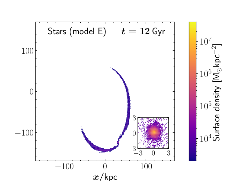
The projected total (DM plus stars) density distribution of the satellite at different times in the simulation is shown in Fig. 3 (left column of panels), for a line of sight parallel to the equatorial plane of the Milky Way. As expected, the initially spherical density distribution of the satellite is distorted by the interaction with the tidal force field of the Milky Way, which produces two significant tidal tails, one leading and one trailing, departing from the main body of the disrupting satellite. However, as illustrated by the zoomed-in surface density maps in the insets in Fig. 3, the central regions remain close to spherical symmetry. While the central total density profile hardly evolves, at larger radii the total density profile changes drastically with time, and at $t=12\,{\rm Gyr}$ (black dashed curve in Fig. 2) it is heavily truncated at $r\approx 1{\rm\,kpc}$ and characterized by a shallow tail at $r\approx 10{\rm\,kpc}$ produced by the stripped particles. To quantify the mass loss we take as reference mass at each time the mass ${M}_{\rm 3\,kpc}$ of all the particles within a sphere of radius $r=3{\rm\,kpc}$ from the centre of the satellite. The choice of $3{\rm\,kpc}$ as reference radius (which is about twice the initial half-mass radius) is somewhat arbitrary, but is empirically motivated by the requirement to include most of the stellar mass at $t=0$ (see Section 5.2.2) and to exclude most of the stellar tidal tails in the subsequent snapshots (see insets in Fig. 3). We note that ${M}_{\rm 3\,kpc}\simeq 0.69{M}_{\rm tot}$ at $t=0$. The black curve in Fig. 4, which plots ${M}_{\rm 3\,kpc}$ as a function of time, shows that, within $3{\rm\,kpc}$, the satellite loses almost $70\%$ of its initial mass over 12 Gyr of evolution.

The simulation is interpreted a posteriori in different ways by choosing different portion functions $\mathcal{P}_{\star}(\mathcal{E})$, where $\mathcal{E}$ is the initial particle relative energy, computed for the isolated satellite. Here we consider two models: model C, in which the initial stellar distribution is more compact, and model E, in which the initial stellar distribution is more extended. Both models are obtained assuming as functional form of $\mathcal{P}_{\star}$ the generalized Schechter function (equation 6). The values of the parameters of $\mathcal{P}_{\star}$ are $\alpha=3$, $\beta=1$, $A=1.35$, and ${\tilde{\mathcal{E}}}_{0}=0.8$ for model C, and $\alpha=0.5$, $\beta=12$, $A=0.5$ and ${\tilde{\mathcal{E}}}_{0}=0.7$ for model E. The initial stellar density profile of model C (red solid curve in upper left panel of Fig. 5) has a central cusp ($\rho_{\star}\propto r^{-1}$) and declines steeply in the outer parts, while the stellar density profile of model E (green solid curve in upper right panel of Fig. 5) has a central core ($\rho_{\star}\propto{\rm constant}$) and is shallower in the outskirts. The position of the knee of the stellar density profile (i.e. the radius of transition between inner and outer slope) occurs at larger radius for model E than for model C.

The stellar and DM density and mass profiles at different times in the simulation are shown in Fig. 5 for model C in the left column of panels and for model E in the right column of panels. In model E the initial DM density is higher than the initial stellar density at all radii. In model C the initial stellar density is higher than the DM density in the centre ($r\lesssim 200{\rm\,pc}$), while the dark halo dominates at larger radii. In both cases the evolution of the DM density profile resembles that of the total mass distribution, with substantial losses at large radii. The evolution of the stellar component is instead very different in the two cases: the stellar distribution of model C remains almost unaltered for 12 Gyr, while it is heavily stripped in model E. The fractional stellar mass loss for the two models is quantified in Fig. 4 using as reference the stellar mass within a sphere of radius $3{\rm\,kpc}$ from the satellite’s centre: over 12 Gyr in model C the satellite loses about $30\%$ of its stellar mass, while in model E more than $70\%$ of the stellar mass is tidally stripped along the orbit. We note that the reference radius $r=3{\rm\,kpc}$ encloses the large majority of the stellar mass at $t=0$ ($98\%$ in model C and $78\%$ in model E), but is small enough to exclude most of the tidal tails during the orbital evolution.

The extent, density and morphology of the stellar tidal tails can be assessed by looking at Fig. 3, showing, for models C (middle column of panels) and E (right column of panels), the projected stellar density distribution of the satellite at different times in the simulation for a line of sight parallel to the Galactic equatorial plane. The stellar streams are extremely tenuous in model C, while are much more pronounced in model E.

Here we study the stellar kinematics of the satellite and of the streams, focusing in particular on the line-of-sight stellar velocity dispersion $\sigma_{\rm los}$. As an illustrative case, we take as line of sight the direction of the $y$ axis in our reference Galactic Cartesian coordinate system and we take as fiducial boundary between the main body of the satellite and the tidal tails $R=3{\rm\,kpc}$, where $R=\sqrt{(x-x_{0})^{2}+(z-z_{0})^{2}}$ is the projected distance from the satellite’s centre $(x_{0},z_{0})$ in the $xz$ plane. For the main body of the satellite we compute $\sigma_{\rm los}$ from sets of particles belonging to circular annuli: the line-of-sight velocity dispersion $\sigma_{{\rm los},j}$ of the $j$-th radial bin $R_{j}<R<R_{j+1}$ is given by

where $v_{y,i}$ is the $y$ component of the velocity of the $i$-th particle, $\left\langle v_{y}\right\rangle=\left(\sum_{i}m_{\star,i}v_{y,i}\right)/\left(\sum_{i}m_{\star,i}\right)$, and the sums are over all particles with $R_{j}<R_{i}<R_{j+1}$. Here $m_{\star,i}=\mathcal{P}_{\star}(\mathcal{E}_{i})m_{i}$, where $m_{i}$ is the mass of the $i$-th particle and $\mathcal{E}_{i}$ is its initial energy in the isolated satellite. Fig. 6 shows the satellite’s initial and final profiles of $\sigma_{\rm los}$ for models C and E. In the initial conditions $\sigma_{\rm los}$ is higher for model E, which has a flatter stellar density profile, than for model C, which has a steeper stellar density profile (see upper panels of Fig. 5). This just reflects the fact that, for a given gravitational potential, a higher velocity dispersion is needed to maintain in equilibrium a more extended stellar component. For both models the final $\sigma_{\rm los}$ profile has a shape similar to the corresponding initial profile, but lower normalization: $\sigma_{\rm los}$ decreases with time mainly because the potential well becomes shallower, owing to substantial mass loss (see Fig. 5, lower panels).

It is also interesting to assess how the kinematics of the stellar tidal tails depends on the initial stellar density distribution. For this purpose we consider the $t=12\,{\rm Gyr}$ snapshot and, taking again the $y$ axis as line of sight, we distinguish the leading tail (lying above and to the right of the satellite in the bottom panels of Fig. 3) and the trailing tail (lying to the left of the satellite in the bottom panels of Fig. 3). Specifically, we assign to the leading tail all particles with $R>3{\rm\,kpc}$ and $z>z_{0}-1.8(x-x_{0})$, and to the trailing tail all particles with $R>3{\rm\,kpc}$ and $z<z_{0}-1.8(x-x_{0})$, with $x_{0}=31.9{\rm\,kpc}$ and $z_{0}=-124.8{\rm\,kpc}$. $\sigma_{\rm los}$ as a function of $R$ is shown in Fig. 7 for the leading and trailing tails of models C and E. For given model, the two tails have similar $\sigma_{\rm los}$ profiles out to $R\approx 40{\rm\,kpc}$: at larger distances form the satellite the leading tail tends to have higher stellar velocity dispersion than the trailing tail. For given tail (leading or trailing), the $\sigma_{\rm los}$ profile is systematically higher for model E than for model C, which reflects the higher velocity dispersion of the stellar component of model E in the initial conditions (Fig. 6). To quantify the overall velocity dispersion of each tail, we compute the quantity $\sigma_{\rm los,tail}$, defined by

where $\sigma_{{\rm los},j}$ and $\Sigma_{\star,j}$ are, respectively, the line-of-sight stellar velocity dispersion and stellar surface density of the $j$-th radial bin of the tail (we used $N_{\rm bin}=24$ bins uniformly spaced in $R$ between $R\simeq 3{\rm\,kpc}$ and $R\simeq 100{\rm\,kpc}$). The leading tail has $\sigma_{\rm los,tail}\simeq 2.8{\rm\,km\,s^{-1}}$ for model C and $\sigma_{\rm los,tail}\simeq 3.6{\rm\,km\,s^{-1}}$ for model E; the trailing tail has $\sigma_{\rm los,tail}\simeq 2.8{\rm\,km\,s^{-1}}$ for model C and $\sigma_{\rm los,tail}\simeq 3.5{\rm\,km\,s^{-1}}$ for model E.

So far we have applied to our simulation two models (C and E), that is two choices of $\mathcal{P}_{\star}$. However, the power of the presented method lies in the fact that infinite models can be explored by varying continuously the values of the parameters of $\mathcal{P}_{\star}$. Thus we illustrate here how some properties of the satellite and of the tails vary in entire family of $n$ models whose extremes are models C and E. The $i$-th member of this family of models (for $i=1,...,n$) has $\mathcal{P}_{\star}(\mathcal{E})$ given by equation (6) with parameters

and

where ($\alpha_{\rm C}$, $\beta_{\rm C}$, $A_{\rm C}$, $\mathcal{E}_{\rm 0,C}$) and ($\alpha_{\rm E}$, $\beta_{\rm E}$, $A_{\rm E}$, $\mathcal{E}_{\rm 0,E}$) are the sets of values of parameters of models C and E, respectively (see Section 5.2.2). With this definition we get model C for $i=1$ and model E for $i=n$; for $1<i<n$ we get models with $\mathcal{P}_{\star}>0$ that are intermediate between models C and E: the stellar component is more embedded in the DM halo for lower values of $i$. Each member of this family of models can be conveniently labelled with the value of its initial ($t=0$) stellar half mass radius $r_{\rm half,\star}$ (that is the radius of the sphere containing half of the stellar mass), which increases monotonically with $i$. The initial stellar density profile of the simulated satellite is shown in Fig. 8 for models C and E, and for three representative intermediate models, labelled with their values of $r_{\rm half,\star}$.

Fig. 9 shows the dependence on $r_{\rm half,\star}$ of some global properties of the stellar component of the simulated satellite for the family of models defined above. The upper panel of Fig. 9 plots the fraction of stellar mass lost (defined as the stellar mass in particles more distant than 3 kpc from the satellite’s centre) as a function of $r_{\rm half,\star}$ after $5\,{\rm Gyr}$ and $12\,{\rm Gyr}$ of evolution. The fraction of stellar mass lost increases smoothly from more embedded (smaller $r_{\rm half,\star}$) to less embedded (larger $r_{\rm half,\star}$) models. The lower panel of Fig. 9 plots the line-of-sight stellar velocity dispersion $\sigma_{\rm los,tail}$ (see Section 5.2.3) of the leading and trailing tails as a function of $r_{\rm half,\star}$. $\sigma_{\rm los,tail}$, which is similar for the two tails for a given model, increases smoothly with $r_{\rm half,\star}$: the less embedded the initial stellar component, the higher the velocity dispersion of the stellar streams.

References

- Battaglia et al. (2015) Battaglia G., Sollima A., Nipoti C., 2015, MNRAS, 454, 2401
- Binney (2014) Binney J., 2014, MNRAS, 440, 787
- Binney & Tremaine (2008) Binney J., Tremaine S., 2008, Galactic Dynamics: Second Edition. Princeton University Press
- Boylan-Kolchin et al. (2006) Boylan-Kolchin M., Ma C.-P., Quataert E., 2006, MNRAS, 369, 1081
- Ciotti & Ziaee Lorzad (2018) Ciotti L., Ziaee Lorzad A., 2018, MNRAS, 473, 5476
- Ciotti et al. (1995) Ciotti L., Stiavelli M., Braccesi A., 1995, MNRAS, 276, 961
- Ciotti et al. (2009) Ciotti L., Morganti L., de Zeeuw P. T., 2009, MNRAS, 393, 491
- Ciotti et al. (2019) Ciotti L., Mancino A., Pellegrini S., 2019, MNRAS, 490, 2656
- Dierickx & Loeb (2017) Dierickx M. I. P., Loeb A., 2017, ApJ, 836, 92
- Eddington (1916) Eddington A. S., 1916, MNRAS, 76, 572
- Evans (1993) Evans N. W., 1993, MNRAS, 260, 191
- Evans (1994) Evans N. W., 1994, MNRAS, 267, 333
- Frigo & Balcells (2017) Frigo M., Balcells M., 2017, MNRAS, 469, 2184
- Hernquist (1990) Hernquist L., 1990, ApJ, 356, 359
- Hiotelis (1994) Hiotelis N., 1994, A&A, 291, 725
- Iorio et al. (2019) Iorio G., Nipoti C., Battaglia G., Sollima A., 2019, MNRAS, 487, 5692
- Johnston et al. (1995) Johnston K. V., Spergel D. N., Hernquist L., 1995, ApJ, 451, 598
- Laporte et al. (2013) Laporte C. F. P., White S. D. M., Naab T., Gao L., 2013, MNRAS, 435, 901
- Laporte et al. (2018) Laporte C. F. P., Johnston K. V., Gómez F. A., Garavito-Camargo N., Besla G., 2018, MNRAS, 481, 286
- Łokas et al. (2010) Łokas E. L., Kazantzidis S., Majewski S. R., Law D. R., Mayer L., Frinchaboy P. M., 2010, ApJ, 725, 1516
- Londrillo et al. (2003) Londrillo P., Nipoti C., Ciotti L., 2003, Memorie della Societa Astronomica Italiana Supplementi, 1, 18
- Merritt (1985) Merritt D., 1985, AJ, 90, 1027
- Nipoti et al. (2003a) Nipoti C., Londrillo P., Ciotti L., 2003a, MNRAS, 342, 501
- Nipoti et al. (2003b) Nipoti C., Stiavelli M., Ciotti L., Treu T., Rosati P., 2003b, MNRAS, 344, 748
- Nipoti et al. (2020) Nipoti C., Cannarozzo C., Calura F., Sonnenfeld A., Treu T., 2020, MNRAS, 499, 559
- Osipkov (1979) Osipkov L. P., 1979, Soviet Astronomy Letters, 5, 42
- Sanders et al. (2018) Sanders J. L., Evans N. W., Dehnen W., 2018, MNRAS, 478, 3879
- Schechter (1976) Schechter P., 1976, ApJ, 203, 297
- Ural et al. (2015) Ural U., Wilkinson M. I., Read J. I., Walker M. G., 2015, Nature Communications, 6, 7599
- Vasiliev (2019) Vasiliev E., 2019, MNRAS, 482, 1525
- Vasiliev et al. (2020) Vasiliev E., Belokurov V., Erkal D., 2020, arXiv e-prints, p. arXiv:2009.10726
- White (1980) White S. D. M., 1980, MNRAS, 191, 1P