Integrability of eccentric, spinning black hole binaries
up to second post-Newtonian order
Abstract
Accurate and efficient modeling of the dynamics of binary black holes (BBHs) is crucial to their detection and parameter estimation through gravitational waves, both with LIGO/Virgo and LISA. General BBH configurations will have misaligned spins and eccentric orbits, eccentricity being particularly relevant at early times. Modeling these systems is both analytically and numerically challenging. Even though the 1.5 post-Newtonian (PN) order is Liouville integrable, numerical work has demonstrated chaos at 2PN order, which impedes the existence of an analytic solution. In this article we revisit integrability at both 1.5PN and 2PN orders. At 1.5PN, we construct four (out of five) action integrals. At 2PN, we show that the system is indeed integrable – but in a perturbative sense – by explicitly constructing five mutually-commuting constants of motion. Because of the KAM theorem, this is consistent with the past numerical demonstration of chaos. Our method extends to higher PN orders, opening the door for a fully analytical solution to the generic eccentric, spinning BBH problem.
I Introduction
To date, Advanced LIGO and Virgo have confidently detected 50 gravitational-wave events Abbott et al. 2016; Abbott et al. 2019; Abbott et al. 2020, all of them from compact binary mergers. Of these, at least 46 are due to a binary black hole (BBH) system. Both detecting and characterizing these systems relies on computing accurate and efficient waveform templates. Present waveform models Ossokine et al. 2020; Khan et al. 2019; Pratten et al. 2020 are already rather sophisticated, including modeling precession due to spin-orbit coupling; but typically, the orbital motion is modeled as quasi-circular, and the precession is approximate (except for NR surrogates Varma et al. 2019). The fact that most eccentricity should be radiated away by the time of merger has been long known Peters and Mathews 1963; Peters 1964. Despite constraints on eccentricity Romero-Shaw et al. 2019, there have been tentative claims that some LIGO events were highly eccentric Gayathri et al. 2020. Moreover with the LISA mission Cutler 1998; Amaro-Seoane et al. 2017 on the horizon, eccentricity is expected to play a more prominent role Roedig and Sesana 2012; Chen and Amaro-Seoane 2017; Fang et al. 2019, and may be especially important for multi-band systems Sesana 2016.
This brings us to the challenge of modeling “generic” BBH systems: two BHs, with their spins misaligned from the orbital angular momentum, in an eccentric orbit. Eccentricity leads to apsidal precession, and spin-orbit coupling leads to precession of both the spins and the orbital plane. Such complicated nonlinear dynamics in a high dimensional phase space leads to the fear of chaos. One ultimate goal of studying the BBH problem is to produce rapid gravitational-wave predictions—and chaos would obstruct the possibility of analytical waveforms. Showing the integrability of the system and the existence of action-angle variables opens the door to constructing a closed-form analytical waveform model.
The study of chaos and integrability in the spinning, eccentric BBH system has an interesting history Levin 2000; Levin 2003; Hughes 2000; Schnittman and Rasio 2001; Cornish and Levin 2003; Schnittman 2004; Hartl and Buonanno 2005; Konigsdorffer and Gopakumar 2005; Wu and Xie 2010; Wu and Zhong 2011; Mei et al. 2013; Huang et al. 2014; Wu and Huang 2015; Huang and Wu 2016. We will recap some of the highlights below. Some of the claims in the literature seem at odds with each other. Besides our main results, we will also explain these apparent contradictions and correct some misstatements in the literature regarding integrability of the BBH system.
The generic BBH system, in Hamiltonian form, has long been known to be integrable at the 1.5 post-Newtonian (PN) order Damour 2001. This comes from the Liouville-Arnold theorem Arnold et al. 2013; José and Saletan 1998: the ten-dimensional phase space has five independent constants of motion, which all pairwise commute under the Poisson bracket. This integrability leads to the existence of an analytic solution Cho and Lee 2019. At 2PN, Levin Levin 2000; Levin 2003 performed numerical simulations and concluded that the generic BBH system is chaotic. Schnittman and Rasio Schnittman and Rasio 2001 also simulated generic systems at 2PN, and by measuring the Lyapunov exponent, found either no chaos, or weak chaos with a Lyapunov time which was many times greater than the inspiral time. Soon after, Cornish and Levin Cornish and Levin 2003 found the Lyapunov and inspiral time-scale could be comparable to each other, though they warned that the Lyapunov time is coordinate-dependent. Hartl and Buonanno Hartl and Buonanno 2005 performed a survey of generic orbits, simulating them at 2PN (and including some PN terms that previous authors had not). For the most part, they found regular (i.e. non-chaotic) orbits, though they did report chaos in some cases, which they reported to be astrophysically disfavored. Though not discussed in any of these works, the coexistence of regular and chaotic orbits in phase space is a typical characteristic of a nearly-integrable system, proven in the KAM theorem Arnold et al. 2013; José and Saletan 1998. This applies to the second and higher PN Hamiltonians, when treated as a perturbation to the integrable 1.5PN Hamiltonian.
There have also been a number of analytical studies of integrability. Damour Damour 2001 pointed out the additional constants of motion, though did not emphasize that they commute or that the generic BBH is integrable. Königsdörffer and Gopakumar Konigsdorffer and Gopakumar 2005; Gopakumar and Konigsdorffer 2005 suggested integrability at higher PN order, by constructing an analytic solution for two specific mass/spin configurations, and removing all spin terms in the Hamiltonian except for the leading order spin-orbit interaction. Beyond the 1.5PN spin-orbit effect, the next non-trivial effect on integrability is the spin-spin interactions at 2PN, which is conjectured to source chaotic behavior Levin 2000. Let us also mention that some analytic work Wu and Xie 2010; Wu and Zhong 2011; Mei et al. 2013; Huang et al. 2014; Wu and Huang 2015; Huang and Wu 2016 has discussed integrability by only counting the number of constants of motion, which is not enough for the Liouville-Arnold theorem: the constants must be mutually commuting. For example, while each of the three components are constants, they do not commute with each other.
Along independent lines, a large body of literature has been developed by taking advantage of orbit-averaging and precession-averaging. The principle at work is that there is a large separation of timescales, ; so the orbital variables’ influence on precession dynamics may be approximated by averaging, and similarly for precession-averaging. Early post-Newtonian works invoking orbit-averaging to study spin effects include Kidder 1995; Schnittman 2004; Racine 2008, and precession-averaging followed in Kesden et al. 2015; Gerosa et al. 2015. An important milestone was Racine’s discovery that a quantity (to be introduced later) is constant under the Newtonian-orbit-average of the 2PN equations of motion (EOMs), despite not being constant under the full 2PN equations. We will briefly comment on the relation of our results to the averaged results.
In this paper, we study the problem of integrability at two levels: we find the action variables at 1.5PN, and show integrability at 2PN. These are both part of the larger program to eventually build analytical waveform models for the generic spinning, eccentric BBH system. The known integrability at 1.5PN implies the existence of action-angle variables. We derive four (out of the five) action variables, with the fourth one being in the form of a PN series. These action variables are closely related to the Keplerian-like parameterization for the generic system at 1.5PN recently presented in Ref. Cho and Lee 2019 (that work omitted the 1PN orbital terms from the Hamiltonian for simplicity, but the approach will work with the 1PN terms included). We then proceed to 2PN, where in the spirit of perturbation theory, we add an ansatz for PN corrections to the 1.5PN exactly-commuting constants, and solve for these corrections to find the 2PN-valid constants. We work with the full 2PN Hamiltonian rather than removing the spin-spin interaction. This shows (via the Liouville-Arnold theorem to be discussed later) that the generic BBH is integrable at 2PN, in the sense of perturbation theory. That is, these 2PN constants only mutually commute up to sufficiently-high-order errors. This also implies that the action variables can be pushed to 2PN, so an analytical orbital solution is possible at this order. We finally revisit the criteria for integrability by analyzing the timescales for “constants” to vary when evolved with the next order Hamiltonian. With this more physical criterion, actually varies at the 1PN timescale, despite being a 1.5PN constant of motion. The 2PN constants we construct only vary at 2.5PN order, justifying that the BBH system is integrable at 2PN order.
The existence of these perturbative constants is not in conflict with the presence of chaos in phase space. From the KAM theorem, most invariant tori will remain unbroken under a sufficiently small perturbation. Resonant tori will be the first to break up into chaotic regions. Our constants are applicable to unbroken tori, which according to Ref. Hartl and Buonanno 2005 fill the vast majority of phase space.
The layout of this paper is as follows. In Sec. II we introduce preliminaries like post-Newtonian power counting, Liouville integrability, the Hamiltonian phase space and Poisson bracket structure for the BBH problem, and the 2PN Hamiltonian. In Sec. III, we compute four out of five action variables up to 1.5 PN by integrating along closed loops on the invariant tori in phase space. In Sec. IV, we give an algebraic definition of PN involution and integrability. We then describe how to systematically construct appropriate ansätze for corrections to add to constants of motion, reducing the problem to linear algebra. Finally we solve for the corrections and present the five approximate constants of motion, which are in involution up to errors that can be ignored at 2PN. In Sec. V, we present our discussion, ideas for future work, and conclude.
II The setup
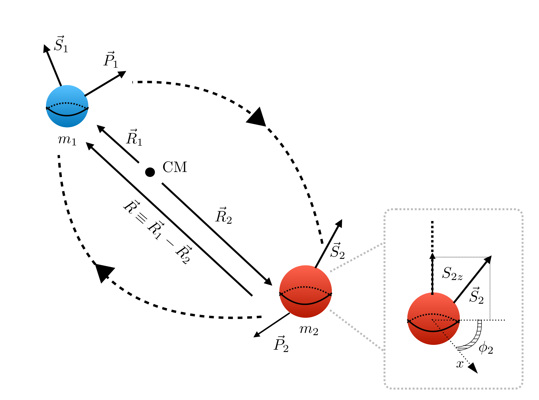
We start by describing the canonical variables and the dynamical setup used to study eccentric binaries of black holes with precessing spins in the PN approximation. The BBH system under consideration is schematically displayed in Fig. 1, using its center-of-mass frame Damour and Schaefer 1988, to define the separation vector and the linear momenta of a binary of black holes with masses and . With these quantities, we build the Newtonian orbital angular momentum , and the total angular momentum which includes the BH spins and . The individual BH masses are and and the total mass . Additionally, the reduced mass is given by and the symmetric mass ratio is a function of the reduced mass. The constants and are used to build the effective spin
| (1) |
This should not be confused with other common spin parameters used in the literature Damour 2001; Racine 2008; Ajith et al. 2011, namely the projected effective spin , or the combination . Racine found Racine 2008 that is conserved under the Newtonian-orbit-average of the 2PN equations of motion; we will discuss this further in Sec. IV.
Even when our approach throughout this paper is purely Hamiltonian, we may define a velocity since the ratio is often used as a PN expansion parameter. Latin indices denote the th Cartesian component of a vector, and we employ the Einstein summation convention unless stated otherwise.
The spin angular momentum for a Kerr black hole labeled is
| (2) |
where so that there are no naked singularities. Notice the factor of , which affects the post-Newtonian order of any terms containing spins; this will be detailed in Secs. II.1 and II.4.
II.1 Counting post-Newtonian orders
Post-Newtonian counting applies to any function of phase-space variables, which we expand as an asymptotic series using a certain PN parameter , i.e. . Depending on context, one of , an orbital frequency , or is used as the expansion parameter. Specifically, from Newtonian order, we may define to be any of
| (3) |
Since we have kept the powers of explicitly, we can see that any choice is equivalent to counting powers of . This latter observation is important when spins are involved, since spin includes [see Eq. (2)] but does not scale with , or .
Let a phase-space function be written in the form
| (4) |
In Eq. (4), is the first non-vanishing term in the expansion, and we would say that the term is PN orders higher than , or is of “relative PN order.” For example, when including spins in the total angular momentum,
| (5) |
we see that spins are 0.5PN orders higher than orbital angular momentum.
II.2 Hamiltonian dynamics on a symplectic manifold
From now on, we will follow the Hamiltonian formulation to study the BBH system; we will shortly review its algebraic structure José and Saletan 1998; Arnold et al. 2013. Hamiltonian dynamics takes place on an (even-dimensional) symplectic manifold. A smooth manifold equipped with a closed non-degenerate differential 2-form (the symplectic form) is called a symplectic manifold. The algebra of non-vanishing Poisson brackets (PBs) between the phase-space variables , and is given by
| (6) |
Notice that all brackets with spins preserve the norms , so although the spin vectors are three-dimensional, each is restricted to evolve on the surface of a 2-sphere. This makes the phase space a ten-dimensional manifold.
Time evolution under a Hamiltonian of any phase-space quantity is given by , where collectively denote canonical coordinates on phase space. The standard rules of sum, product, anti-commutativity, and chain rule make the PBs in Eq. (6) sufficient to evaluate the PB of any quantities built from .11 1 If computing PBs by hand, the following derived identities are also useful: ; and, for any scalar function , , where the 3-vector has components , and similarly for . The remainder of this section is for readers interested in the symplectic structure, relevant to computing action-angle variables, the subject of Sec. III.
Our symplectic manifold is the product of the 6-dimensional phase space of orbital dynamics, and two 2-dimensional spin phase spaces, each of which is an (the only that admits a symplectic structure). The symplectic form is correspondingly a sum over the three manifolds. Commonly, symplectic forms are presented in Darboux coordinates,
| (7) |
This is possible on the orbital phase space, which is a cotangent space, , and admits the globally-valid canonical form .
However, there is no globally-valid Darboux coordinate system on the 2-sphere. The symplectic structure on the is unique up to scaling and is proportional to the standard area element, ; the normalization is fixed to agree with Eq. (6). Thinking of the as an embedded submanifold in spin space, the inverse symplectic form can be written as
| (8) |
This representation should make it clear that the symplectic form is SO(3) covariant. An equivalent representation is , where is the azimuthal angle of the spin about the axis. The total symplectic form is thus
| (9) |
As noted above, it is SO(3) covariant, which will be useful in evaluating some action integrals. Finally let us note that while is -independent, while carries one power of spin [seen in Eqs. (6) and (8)], and spin carries a power of . Orbital and spin PBs thus change PN orders in different ways, which will be important in Sec. IV.
II.3 Integrable systems
A -dimensional Hamiltonian system is said to be integrable in the Liouville sense if there exist independent phase-space functions which are all mutually Poisson commuting, . These functions are said to be “in involution” Fasano et al. 2006; Arnold et al. 2013; José and Saletan 1998.22 2 More precisely, the Liouville-Arnold theorem states that, on a -dimensional symplectic manifold, if and there are independent phase-space functions in mutual involution, and if level sets of these functions form a compact and connected manifold, then the system is integrable. Bound systems that are integrable admit a canonical transformation to a set of phase-space coordinates called action-angle variables. The evolution of such systems is trivial in action-angle variables, so there cannot be any chaos or phase space mixing; all bound orbits are multiply-periodic. Action-angle variables are ideal for studying perturbations of integrable systems. For our purposes, we would like to treat terms of higher PN orders as a perturbation of an integrable system.
A level set of all the constants of motion must be an -dimensional torus Arnold et al. 2013. The actions can be found via certain coordinate-independent integrals along closed loops restricted to the tori (holding constant each of the ). If global Darboux coordinates are possible, the action integrals are Fasano et al. 2006; Arnold et al. 2013; José and Saletan 1998,
| (10) |
Here is the th loop on the torus. The set of loops must be in different homotopy classes (more precisely, the homotopy classes form an integer lattice , and our loops’ homotopy classes must span the lattice). The 1-form integrand of Eq. (10) is a symplectic potential, , whose exterior derivative gives the symplectic 2-form, . Since is closed, it is straightforward to show that the depend only on homotopy class, and not on choice of loop in that class.
However on some symplectic manifolds, including the 2-sphere, is not an exact form, . This makes the action integrals Eq. (10) ambiguous. One approach is to make a global choice of how to ‘cap’ the loops to another reference loop, and thus perform integrals of over 2-surfaces. This ambiguity is benign, as it will only shift the action integrals by global constants.33 3 We thank Samuel Lisi for discussion of the finer points of this ambiguity.
To complete the coordinate system, there will be angle variables which are conjugate, i.e. and all other PBs vanishing. Each angle variable runs from 0 to as one follows the flow generated by its conjugate action. We will not construct the angle variables in this work.
II.4 2PN Hamiltonian with spins included
To write the Hamiltonian at different post-Newtonian orders, we adopt the convention that stands for the part of Hamiltonian which is of PN order relative to the leading Newtonian order term (dubbed ). The Hamiltonian up to 2PN of the BBH system in the center-of-mass frame is
| (11) |
where represents corrections of order 2.5PN and higher. To simplify we will use the scaled quantities , , and the radial component of scaled momentum is , with the implicit understanding that the “hatted” version of any vector in this paper is the corresponding unit vector. The vector has units of velocity, and has units of velocity squared, enabling the easy reading of PN orders. The individual contributions are Barker et al. 1966; Damour 2001; Barker and O’Connell 1975; Hartl and Buonanno 2005; Steinhoff 2011
| (12) | ||||
| (13) | ||||
| (14) | ||||
| (15) |
The 2PN spin-spin interaction is
| (16) | ||||
| (17) | ||||
| (18) | ||||
| (19) |
where is symmetric and trace-free.
Notice that since and, as previously mentioned, spin goes as , so indeed . Likewise, , justifying the claimed PN orders of these terms.
III Action variables at 1.5PN order
To start, we will focus on integrability at 1.5PN, truncating the Hamiltonian to
| (20) |
As has been known for many years now Damour 2001, truncating at this order gives a 10-dimensional phase space with 5 constants of motion in mutual involution, namely, the set . At this level, the involution is “exact,” for the associated PBs vanish exactly. This involution can be verified by the Mathematica notebook which accompanies this article Mma, which makes use of the xAct/xTensor suite JMM; Martín-García 2008.
This involution implies the existence of action-angle variables. We will construct four out of five action variables in this section. For each action variable , we will consider a different loop tangent to the five-torus given by constancy of the five , and perform the (capped) loop integral of Eq. (10).
III.1 Loops generated by , and
We find three of these loops by following the flow of the generators , and . To demonstrate, let be the vector field tangent to the flow generated by . Notice that this flow makes and rigidly rotate about the constant , while the two are not moved. Thus we have (with representing either or )
| (21) |
As this is a rigid rotation, the phase-space flow will complete one cycle as the parameter increases by . Similarly, let . This time all vectors rotate rigidly about the axis,
| (22) |
with representing any of and . After increases by , the spin and orbital phase-space variables will close the loop. Thirdly, with , all vectors rigidly rotate around the constant ,
| (23) |
with again representing any of and . The phase-space flow under closes after the parameter increases by .
All three of these flows can be treated with the same method. Since the symplectic forms on orbital and spin phase spaces simply add, we treat the orbital and spin components one at a time and add the final results,
| (24) | ||||
| (25) |
and similarly for the spin sector, except that the spin integral is ‘capped’ so as to become an area integral of .
We write for any of the three flows, and use to denote the fixed vector about which others rotate, being one of . The loop closes after the parameter change of . This is illustrated in Fig. 2. The only exception is that the spin vectors are not moved by , but since we break the action integral up as in Eq. (24), this is simple to implement. First, when we parameterize using , the integral becomes
| (26) |
The second equality comes from evaluating the flow for ; the third equality comes from permuting the triple product. The last equality arises since in all three cases, rigidly rotates around (because and also rigidly rotate around ), so the dot product is constant around the loop.
For the spin sector, we choose to cap each curve by the equatorial plane (in spin space), i.e. the oriented area integral will be bounded between the plane and . One can show that this gives the same result as the ordinary integral (for one of the two spins)
| (27) |
While this integral does not seem to be SO(3) covariant, recall that the symplectic form does have this symmetry, as seen in Eq. (8). To take advantage of this symmetry, we call a new axis , and instead compute . Since each rigidly rotates around , the integral in one spin sector will simply be
| (28) |
Combining, we see for the generators and ,
| (29) |
Meanwhile, for , only the orbital sector contributes, and we have . This gives us our first three action integrals,
| (30) |
III.2 Loop in - space
To compute a fourth action variable, we find a loop on the five-torus (of constant values of the mutually-commuting phase-space functions) in a plane parallel to the - plane. We will denote the constant values of the functions with overbars, i.e. taking the values , and . We define to be the momentum conjugate to the radial separation ,
| (31) |
To show how to construct this loop, we eliminate from the 1.5PN Hamiltonian all dependence except for , and the values of constants. This starts from the definition of , to get
| (32) | ||||
| (33) |
Replacing using this relation will eliminate the angular components of from the 1.5PN Hamiltonian. To compact the notation, we will again use the scaled variables , with , and define the shorthand
| (34) |
which is the Newtonian kinetic energy per reduced mass (and also has units of ). Then evaluating the 1.5PN Hamiltonian on this torus, we find
| (35) |
This equality demonstrates that we can solve for in terms of , and – thus making a loop while staying tangent to the torus. We solve for perturbatively in powers of , finding
| (36) |
Here we have collected terms by powers of , in anticipation of performing a Sommerfeld integral, following Damour and Schäfer Damour and Schaefer 1988. This momentum enters into the action integral, where the loop is restricted to the plane,
| (37) |
where the coefficients are constants along this loop, to be read directly from Eq. (36). The factor of 2 comes since the loop runs from one turning point, , to the other, , and then back.
To evaluate this integral, we can use the results from Sec. 3 (or Appendix B) of Damour and Schaefer 1988. The result is in terms of the torus constants , and . We promote these back to their respective phase-space functions, giving
| (38) |
Unlike the first three actions, the fourth action is not “exact” at 1.5PN, but rather we have presented it as a PN series, just like the radial action in Ref. Damour and Schaefer 1988. This is consistent with the 1.5PN Hamiltonian itself being a truncated PN series.
The four action integrals we computed are functionally independent, as can be seen by their different dependence on the original mutually-commuting phase-space functions , and . This corresponds to their loops (all of which are tangent to a torus) being in linearly-independent homology classes. The calculations for the fifth action (both as a PN series and “exact” at the 1.5PN order) are quite lengthy, so we will present them in future work.
It is worth noting that at 1.5PN order, spin effects enter the action integrals, as can be easily seen in Eqs. (30) and (38). This is relevant to the method of torus-averaging, which is used in canonical perturbation theory Goldstein et al. 2013; José and Saletan 1998. Since the actions depends on spin, it is easy to see that torus-averaging will differ from orbit-averaging (over Newtonian orbits) which has been used extensively in the literature Kidder 1995; Schnittman 2004; Racine 2008; Kesden et al. 2015; Gerosa et al. 2015. We expect torus-averaging to be more accurate at 1PN and higher orders.
IV Integrability at 2PN
The spirit of the post-Newtonian method is perturbation theory in powers of , which opens the door for canonical perturbation theory applied to Hamiltonian dynamics. As the KAM theorem dictates Goldstein et al. 2013; José and Saletan 1998, when we add a small perturbation to an integrable system, and this perturbation breaks integrability, the perturbed motion is still multiply-periodic and restricted to -tori, except for resonant tori where chaos ensues.44 4 The KAM theorem actually gives more precise estimates for the dependence of the chaotic component of phase space; see Ref. José and Saletan 1998 for more details.
We can take advantage of perturbation theory by treating the 2PN system as a perturbation upon the 1.5PN Hamiltonian. We find deformations to the 1.5PN constants of motion such that the 2PN system is integrable in the perturbative sense. This method can be pushed to higher PN order, but here we only demonstrate it at the first order where “exact” integrability is broken, namely at the 2PN order. In Sec. IV.1 we explain what we mean by perturbative integrability, and in Sec. IV.2 the method for finding the deformations to the constants. In Sec. IV.3 we give the results for the deformed constants, and discuss some subtle issues in PN integrability in Sec. IV.4.
IV.1 Perturbative integrability
To make the definition of perturbative integrability precise, we will introduce the “dominant PN order of” symbol . If a phase-space quantity is asymptotic to , then it has dominant PN order , i.e.
| (39) |
where is a -independent phase-space function, and we employ the symbol of asymptotic analysis Bender and Orszag 1999. The algebra of formal power series tells us how interacts with multiplication, addition, and thus Poisson brackets. Multiplication is simple,
| (40) |
When two phase-space functions have different dominant orders, addition is also simple,
| (41) |
However, if , then there will be a cancellation in the dominant order of , and the dominant order of the sum will be higher than . Such cancellation can happen in Poisson brackets, and is necessary for our algebraic definition of perturbative integrability.
In perturbation theory, equalities only need to be satisfied up to some sufficiently-small error terms. Thus for perturbative integrability, we will replace with conditions , for some appropriate PN orders . If we want perturbative integrability at relative PN order, we know we want each to be at least a factor of higher than some phase-space quantity, but what is that quantity?
To answer this question, we define the function which measures what would be the “expected” dominant PN order of if there was no cancellation in the leading order (“dominant non-commutation”). This expected order has two cases, corresponding to the leading orders of and both contain a common spin vector or not. This is because the (inverse) symplectic form for spins itself carries a power of and thus [see Eq. (8)]. Thus we define
If and do not have cancellation at the leading order, we see that . For example, , but for .
If exactly, then and are said to be in involution up to infinite order. Otherwise we say that and are in involution “up to PN order” when the two equivalent conditions hold,
| (42a) | ||||
| (42b) | ||||
As a consistency check, notice that for the previous examples and with , each pair is not in involution even at the leading (0PN) order, as would be expected. Now we define a “PN constant of motion” to be a quantity which is in involution with the PN Hamiltonian up to at least PN order. Finally, we define PN perturbative integrability in a -dimensional phase space when we have independent phase-space functions (including the PN Hamiltonian) which are in mutual involution up to at least PN order. We will revisit this definition further in Sec. IV.4, and see that it has a shortcoming.
IV.2 Method of finding deformations
We now construct perturbative constants of motion up to 2PN. Note that and always remain exact constants of motion, at any order, for an SO(3)-invariant Hamiltonian. Along with the Hamiltonian, they form a set of three independent mutually commuting constants of motion. We need to add two more quantities to this list to establish integrability. We propose that the two required constants of motion are perturbative deformations of the 1.5PN constants of motion, and , namely
| (43) | ||||
| (44) |
where and are higher-PN corrections that we must find. For every pair, we want involution up to 2PN order [ in Eq. (42)]. The dominant orders of each of these functions are and . Therefore, to satisfy 2PN perturbative integrability, we require
| (45a) | ||||
| (45b) | ||||
| (45c) | ||||
where is the 2PN Hamiltonian.
Satisfying these integrability conditions amounts to finding the deformations and , which both proceed following the same approach. First, the PN orders that are required to appear in a deformation are identified. Then we construct an ansatz for the deformation out of geometrical objects at these required PN orders, times some coefficients to be determined by Eqs. (45). This turns the problem into a systematic enumerative algebra problem.
At first glance it may seem that this procedure is not systematic, as there are an infinite number of terms that could appear in such an ansatz at fixed PN order, but this is not true. First, the only quantities that may appear are geometric objects transforming covariantly under SO(3) rigid rotations:
- •
the metric tensor (Kronecker delta),
- •
Levi-Civita tensor (not the symbol) ,
- •
the position vector , its norm and unit radial vector ,
- •
momentum vector , and
- •
spin vectors (, ).
In practice, it is simpler to construct such ansätze from and powers of the scalar , rather than considering . SO(3) covariance requires that these objects automatically commute with and . The types of terms allowed in a deformation have the same tensorial character and parity (scalar, pseudoscalar, vector, etc.) as the quantity being corrected. While negative powers can appear in PN expressions, negative powers of or do not. Now, if we choose a maximum operator order (number of tensors multiplied together), there are only a finite number of combinations that can be built at each PN order and operator order. Now the problem is indeed enumerative: if a solution is not found, increase the operator order and try again.
Let us demonstrate by using as an example. First, we determine the PN orders necessary for the ansatz of the deformation . Expanding Eq. (45a),
| (46) |
The noncommutation in the first term on the RHS is only with the spin-spin term, since commutes with the orbital part,
| (47) |
This is the dominant error that must be cancelled by the terms involving , which we see must involve spins. The bracket of with the Hamiltonian also follows PN ordering and is dominated by , with the other terms being higher-PN. One must be careful to check what happens with the spin terms, which potentially reduce PN orders: for example since has spins in its leading order, is only 1PN order higher than , rather than 1.5PN. Therefore this condition simplifies to
| (48) |
with the equality being exact. To satisfy this, will need to contain two spin in the leading order, which by inspection must be .
To build an appropriate ansatz for , we note from Eq. (3) that a factor of should accompany either two powers of , or one power of , and any number of powers of . Since is parity even, we will not use to construct the ansatz for : an odd number of ’s makes a parity odd term, and an even number can be written in terms of . This yields an ansatz containing terms of the form
| (49) |
Here we mean to take all possible contractions of the two tensorial forms, where the indices label spins in the same way as in Sec. II. This leads to 19 possible contractions involving two factors of , and 6 contractions without , giving us altogether terms in our most general ansatz for . Since we are taking contractions, the use of the metric tensor is implicit in our ansatz construction. Our ansatz for then consists of a sum of all these 25 terms with coefficients to be solved for demanding that Eq. (48) be true.
One can employ similar lines of reasoning to construct an ansatz for and solve for the coefficients so that Eq. (45b) is satisfied, although it is a more complicated case than for . Instead of Eq. (48), this time we demand that Eq. (57) be satisfied in the next section. Finally, there may be additional constraints on the terms in the ansätze arising from the requirement that the Poisson bracket must also vanish to the required order, Eq. (45c). That is how we finally arrive at the desired and . We formed sufficiently general ansätze using the AllContractions and MakeAnsatz commands of the Mathematica package xTras Nutma 2014, which works in the xAct/xTensor suite JMM; Martín-García 2008. Our result may be verified by the Mathematica notebook which accompanies this article Mma.
IV.3 The deformed constants
Following the above procedure to find a deformation to , we write this deformation as
| (50) |
For brevity we will define the symmetric tensor
| (51) |
where we again used the scaled variables , . Notice that has units of , and that the trace is
| (52) |
Then we can write our deformation as
| (53) | ||||
We are also free to add arbitrary constants times and without affecting integrability.
Proceeding similarly for , we decompose the deformation as
| (54) |
The two deformations are
| (55) |
| (56) |
We are also free to add arbitrary constants times , and without affecting integrability. The cancellations happen as
| (57) |
with the equality being exact, where is defined in Eq. (16). Below every Poisson bracket, we indicate both the PN orders arising, and what kind of PBs (orbital or spin) are needed to expand each term. With these corrections, we have fulfilled the required level of commutation given in Eqs. (45). In fact, we slightly exceeded this goal, achieving
| (58a) | ||||
| (58b) | ||||
| (58c) | ||||
Therefore, along with the 2PN Hamiltonian , and , the deformed constants and now form a set of 5 independent, mutually commuting constants of motion at 2PN order, thereby establishing the integrable nature of the BBH system at this order.
It is worth comparing our results to the widely-used results based on orbit-averaging (over a Newtonian orbit) Kidder 1995; Schnittman 2004; Racine 2008; Kesden et al. 2015; Gerosa et al. 2015. Racine found Racine 2008 that the combination is conserved by what we call , the Newtonian-orbit average of the 2PN EOMs. Here was introduced by Damour Damour 2001. Two comments are in order. First, differs at its leading order from and therefore . Since spins and are all constants at Newtonian order, applying the Newtonian-orbit-average to form does not recover . Second, as mentioned at the end of Sec. III, a more accurate average is not over the Newtonian orbit, but on the phase-space torus formed by level sets of the five constants of motion. The torus-average will already differ at 1PN order from the Newtonian-orbit average. We can confirm using the 2PN Hamiltonian and averaging over the Newtonian orbit the two independent equalities,
| (59) |
However, we should expect that the torus-average will differ. More precisely, with the 2PN Hamiltonian and no averaging,
| (60) |
Thus while Newtonian-orbit averaging gives a cancellation of this leading order, we expect the more accurate torus average to be nonzero at the order
| (61) |
Notice this is the same level of conservation that we achieved in Eq. (58b), but our result is valid instantaneously, that is, without resorting to averaging.
IV.4 PN constancy and integrability revisited
Our algebraic definition of PN involution and integrability introduced in Sec. IV.1 has a shortcoming. To understand this, let’s examine the timescales on which phase-space quantities vary. For some quantity , when evolved with the full PN Hamiltonian (not the PN contribution to the Hamiltonian), we can approximate the timescale of variation with
| (62) |
For example, the orbital (or Newtonian) timescale is
| (63) |
Now, with the algebraic definition of PN integrability given in Sec. IV.1, is a 1.5PN constant of motion. But let us examine the timescale of its variation, in units of the orbital time. We cannot use for this, since and commute. The timescale of variation is controlled by the 2PN Hamiltonian, and one can check
| (64) |
implying that varies on a timescale that is only 1.5PN longer than , rather than the expected 2PN orders longer. Therefore, is not a 1.5PN constant from the criterion of comparing timescales, and the BBH system cannot yet be called integrable at 1.5PN order despite the existence of five exactly commuting constants at this order.
The key point is that may sometimes induce variations in a quantity at a timescale which is only PN orders larger than , rather than PN orders larger. As was emphasized in Secs. II.1, II.2, and IV.1, this happens because of the factor of in spin, and the form of the spin Poisson bracket. Therefore, to establish if a quantity is a constant of motion on an PN timescale will generally involve examining the PN Hamiltonian.
To conservatively satisfy the timescale analysis, we revise the earlier definition of PN constancy and integrability by using the next order, PN, Hamiltonian, instead of the PN Hamiltonian. However, we only introduce relative PN corrections to our deformed constants. We have checked that the five quantities and ( now being the 2.5PN Hamiltonian Steinhoff 2011) are also in mutual involution up to 2PN according to our revised definition, even though the last two quantities were derived in Sec. IV.2 by only considering the 2PN Hamiltonian. This calculation is also verified in the supplement to this article Mma. In terms of timescales, we now satisfy
| (65) |
Hence, we have established the integrable nature of the BBH system at one PN order higher (2PN) than what was earlier known (1PN) on the basis of timescale of variation.
V Discussion
In this paper, we studied the problem of integrability at two levels: 1.5PN and 2PN. At 1.5PN, where exact integrability had already been known Damour 2001, we evaluated four (out of five) action variables, with the fourth one being a perturbative PN series. At 2PN order, by adding corrections to the 1.5PN mutually commuting constants of motion, we constructed 2PN perturbatively commuting quantities. This proves the integrable nature of the BBH system at 2PN in a perturbative sense. Our construction required us to propose appropriate definitions of PN involution and integrability. Proving perturbative integrability at 2PN and higher is more delicate than at 1.5PN, since the 1.5PN commutation does not require perturbation theory. We presented a systematic method to find higher-PN corrections to mutually commuting constants of motion, forming an ansatz by enumerating possible tensor expressions, turning the problem into linear algebra. We therefore expect our method to be useful in extending integrability to even higher PN orders.
By now a large number of authors have studied the problems of integrability or chaos in the BBH system in post-Newtonian theory, either numerically or analytically. Importantly, while Hartl and Buonanno Hartl and Buonanno 2005 did find chaos in the PN BBH system, they found it is only present in a small component of phase space. The constants of motion we have constructed apply to the invariant tori in the non-chaotic regions of phase space, i.e. the majority of the volume. This improves the outlook for using perturbative integrability as a tool for generating highly-accurate and efficient waveform models.
To employ integrability for efficient waveform modeling, the current work will have to be extended in a number of natural ways. We plan to present the exact (at 1.5PN) fifth action variable and its PN expansion in a future article, also yielding all the frequencies of the system in closed form. Work still needs to be done towards finding the angle variables. These action-angle variables are related to the recent Keplerian-like solution for the eccentric, spinning BBH system at 1.5PN Cho and Lee 2019. These action-angle variables can be pushed to 2PN order and beyond via perturbation methods. This will fail for the small chaotic region of phase space, and more care will be needed near resonances.
This opens the possibility to construct an analytic waveform model for the completely generic system, without needing to e.g. orbit-average Kidder 1995; Schnittman 2004; Racine 2008, precession-averaging Kesden et al. 2015; Gerosa et al. 2015; Khan et al. 2019; Pratten et al. 2020, or expand in powers of eccentricity Klein and Jetzer 2010; Klein et al. 2018. As discussed at the end of Sec. IV.3, we expect the time derivatives of the orbit-averaged constants to have errors at relative 2.5PN order, when averaged over the true orbits, rather than over Newtonian orbits. This is the same level of error in the time derivatives of our instantaneous constants, i.e. without needing to average. We hope to see our integrability results applied to future analytical waveform models such as the Phenom family.
A difficulty will arise at 2.5PN order, where the dynamics are no longer conservative. Starting at this order, the “constants” of motion will now vary with time. One possible approach will be the formalism of non-conservative classical dynamics Galley 2013; Galley et al. 2014; Galley and Rothstein 2017; Tsang et al. 2015, which has a Hamiltonian version. Even if the non-conservative approach proves difficult, the conservative sector of the dynamics can still be pushed to higher PN order, and the time-evolution of the “constants” imposed afterwards through order reduction.
Acknowledgements.
We would like to thank Samuel Lisi and Clifford Will for helpful discussions, and Davide Gerosa for the initial motivation to investigate post-Newtonian spin dynamics that eventually led to this work. The work of JG was partially supported by the Natural Sciences and Engineering Research Council of Canada (NSERC), funding reference #CITA 490888-16, #RGPIN-2019-07306.References
- Abbott et al. (2016) B.P. Abbott et al. (LIGO Scientific, Virgo), “Observation of Gravitational Waves from a Binary Black Hole Merger,” Phys. Rev. Lett. 116, 061102 (2016), arXiv:1602.03837 [gr-qc] .
- Abbott et al. (2019) B.P. Abbott et al. (LIGO Scientific, Virgo), “GWTC-1: A Gravitational-Wave Transient Catalog of Compact Binary Mergers Observed by LIGO and Virgo during the First and Second Observing Runs,” Phys. Rev. X 9, 031040 (2019), arXiv:1811.12907 [astro-ph.HE] .
- Abbott et al. (2020) R. Abbott et al. (LIGO Scientific, Virgo), “GWTC-2: Compact Binary Coalescences Observed by LIGO and Virgo During the First Half of the Third Observing Run,” (2020), arXiv:2010.14527 [gr-qc] .
- Ossokine et al. (2020) Serguei Ossokine et al., “Multipolar Effective-One-Body Waveforms for Precessing Binary Black Holes: Construction and Validation,” Phys. Rev. D 102, 044055 (2020), arXiv:2004.09442 [gr-qc] .
- Khan et al. (2019) Sebastian Khan, Katerina Chatziioannou, Mark Hannam, and Frank Ohme, “Phenomenological model for the gravitational-wave signal from precessing binary black holes with two-spin effects,” Phys. Rev. D 100, 024059 (2019), arXiv:1809.10113 [gr-qc] .
- Pratten et al. (2020) Geraint Pratten et al., “Let’s twist again: computationally efficient models for the dominant and sub-dominant harmonic modes of precessing binary black holes,” (2020), arXiv:2004.06503 [gr-qc] .
- Varma et al. (2019) Vijay Varma, Scott E. Field, Mark A. Scheel, Jonathan Blackman, Davide Gerosa, Leo C. Stein, Lawrence E. Kidder, and Harald P. Pfeiffer, “Surrogate models for precessing binary black hole simulations with unequal masses,” Phys. Rev. Research. 1, 033015 (2019), arXiv:1905.09300 [gr-qc] .
- Peters and Mathews (1963) P.C. Peters and J. Mathews, “Gravitational radiation from point masses in a Keplerian orbit,” Phys. Rev. 131, 435–439 (1963).
- Peters (1964) P.C. Peters, “Gravitational Radiation and the Motion of Two Point Masses,” Phys. Rev. 136, B1224–B1232 (1964).
- Romero-Shaw et al. (2019) Isobel M. Romero-Shaw, Paul D. Lasky, and Eric Thrane, “Searching for Eccentricity: Signatures of Dynamical Formation in the First Gravitational-Wave Transient Catalogue of LIGO and Virgo,” Mon. Not. Roy. Astron. Soc. 490, 5210–5216 (2019), arXiv:1909.05466 [astro-ph.HE] .
- Gayathri et al. (2020) V. Gayathri, J. Healy, J. Lange, B. O’Brien, M. Szczepanczyk, I. Bartos, M. Campanelli, S. Klimenko, C. Lousto, and R. O’Shaughnessy, “GW190521 as a Highly Eccentric Black Hole Merger,” (2020), arXiv:2009.05461 [astro-ph.HE] .
- Cutler (1998) Curt Cutler, “Angular resolution of the LISA gravitational wave detector,” Phys. Rev. D 57, 7089–7102 (1998), arXiv:gr-qc/9703068 .
- Amaro-Seoane et al. (2017) Pau Amaro-Seoane et al. (LISA), “Laser Interferometer Space Antenna,” (2017), arXiv:1702.00786 [astro-ph.IM] .
- Roedig and Sesana (2012) Constanze Roedig and Alberto Sesana, “Origin and Implications of high eccentricities in massive black hole binaries at sub-pc scales,” J. Phys. Conf. Ser. 363, 012035 (2012), arXiv:1111.3742 [astro-ph.CO] .
- Chen and Amaro-Seoane (2017) Xian Chen and Pau Amaro-Seoane, “Revealing the formation of stellar-mass black hole binaries: The need for deci-Hertz gravitational wave observatories,” Astrophys. J. Lett. 842, L2 (2017), arXiv:1702.08479 [astro-ph.HE] .
- Fang et al. (2019) Xiao Fang, Todd A. Thompson, and Christopher M. Hirata, “The Population of Eccentric Binary Black Holes: Implications for mHz Gravitational Wave Experiments,” Astrophys. J. 875, 75 (2019), arXiv:1901.05092 [astro-ph.HE] .
- Sesana (2016) Alberto Sesana, “Prospects for Multiband Gravitational-Wave Astronomy after GW150914,” Phys. Rev. Lett. 116, 231102 (2016), arXiv:1602.06951 [gr-qc] .
- Levin (2000) Janna J. Levin, “Gravity waves, chaos, and spinning compact binaries,” Phys. Rev. Lett. 84, 3515 (2000), arXiv:gr-qc/9910040 .
- Levin (2003) Janna J. Levin, “The fate of chaotic binaries,” Phys. Rev. D 67, 044013 (2003), arXiv:gr-qc/0010100 .
- Hughes (2000) Scott A. Hughes, “Comment on ‘Gravity waves, chaos, and spinning compact binaries’,” Phys. Rev. Lett. 85, 5480 (2000), arXiv:gr-qc/0101024 .
- Schnittman and Rasio (2001) Jeremy D. Schnittman and Frederic A. Rasio, “Ruling out chaos in compact binary systems,” Phys. Rev. Lett. 87, 121101 (2001), arXiv:gr-qc/0107082 .
- Cornish and Levin (2003) Neil J. Cornish and Janna J. Levin, “Lyapunov timescales and black hole binaries,” Class. Quant. Grav. 20, 1649–1660 (2003), arXiv:gr-qc/0304056 .
- Schnittman (2004) Jeremy D. Schnittman, “Spin-orbit resonance and the evolution of compact binary systems,” Phys. Rev. D70, 124020 (2004), arXiv:astro-ph/0409174 [astro-ph] .
- Hartl and Buonanno (2005) Michael D. Hartl and Alessandra Buonanno, “The Dynamics of precessing binary black holes using the post-Newtonian approximation,” Phys. Rev. D 71, 024027 (2005), arXiv:gr-qc/0407091 .
- Konigsdorffer and Gopakumar (2005) Christian Konigsdorffer and Achamveedu Gopakumar, “Post-Newtonian accurate parametric solution to the dynamics of spinning compact binaries in eccentric orbits: The Leading order spin-orbit interaction,” Phys. Rev. D 71, 024039 (2005), arXiv:gr-qc/0501011 .
- Wu and Xie (2010) Xin Wu and Yi Xie, “Symplectic structure of post-Newtonian Hamiltonian for spinning compact binaries,” Phys. Rev. D 81, 084045 (2010), arXiv:1004.4549 [gr-qc] .
- Wu and Zhong (2011) Xin Wu and Shuang-Ying Zhong, “Regular dynamics of canonical post-Newtonian Hamiltonian for spinning compact binaries with next-to-leading order spin-orbit interactions,” General Relativity and Gravitation 43, 2185–2198 (2011).
- Mei et al. (2013) Lijie Mei, Mingjie Ju, Xin Wu, and Sanqiu Liu, “Dynamics of spin effects of compact binaries,” Mon. Not. Roy. Astron. Soc. 435, 2246–2255 (2013).
- Huang et al. (2014) Guoqing Huang, Xiaoting Ni, and Xin Wu, “Chaos in two black holes with next-to-leading order spin-spin interactions,” Eur. Phys. J. C 74, 3012 (2014), arXiv:1403.0378 [gr-qc] .
- Wu and Huang (2015) Xin Wu and Guoqing Huang, “Ruling out chaos in comparable mass compact binary systems with one body spinning,” Mon. Not. Roy. Astron. Soc. 452, 3167–3178 (2015).
- Huang and Wu (2016) Li Huang and Xin Wu, “Second post-Newtonian Lagrangian dynamics of spinning compact binaries,” Eur. Phys. J. C 76, 488 (2016), arXiv:1604.05810 [gr-qc] .
- Damour (2001) Thibault Damour, “Coalescence of two spinning black holes: an effective one-body approach,” Phys. Rev. D 64, 124013 (2001), arXiv:gr-qc/0103018 .
- Arnold et al. (2013) V.I. Arnold, K. Vogtmann, and A. Weinstein, Mathematical Methods of Classical Mechanics, Graduate Texts in Mathematics (Springer New York, 2013).
- José and Saletan (1998) J.V. José and E.J. Saletan, Classical Dynamics: A Contemporary Approach (Cambridge University Press, 1998).
- Cho and Lee (2019) Gihyuk Cho and Hyung Mok Lee, “Analytic Keplerian-type parametrization for general spinning compact binaries with leading order spin-orbit interactions,” Phys. Rev. D100, 044046 (2019), arXiv:1908.02927 [gr-qc] .
- Gopakumar and Konigsdorffer (2005) Achamveedu Gopakumar and Christian Konigsdorffer, “The Deterministic nature of conservative post-Newtonian accurate dynamics of compact binaries with leading order spin-orbit interaction,” Phys. Rev. D 72, 121501(R) (2005), arXiv:gr-qc/0511009 .
- Kidder (1995) Lawrence E. Kidder, “Coalescing binary systems of compact objects to postNewtonian 5/2 order. 5. Spin effects,” Phys. Rev. D 52, 821–847 (1995), arXiv:gr-qc/9506022 .
- Racine (2008) Etienne Racine, “Analysis of spin precession in binary black hole systems including quadrupole-monopole interaction,” Phys. Rev. D78, 044021 (2008), arXiv:0803.1820 [gr-qc] .
- Kesden et al. (2015) Michael Kesden, Davide Gerosa, Richard O’Shaughnessy, Emanuele Berti, and Ulrich Sperhake, “Effective potentials and morphological transitions for binary black-hole spin precession,” Phys. Rev. Lett. 114, 081103 (2015), arXiv:1411.0674 [gr-qc] .
- Gerosa et al. (2015) Davide Gerosa, Michael Kesden, Ulrich Sperhake, Emanuele Berti, and Richard O’Shaughnessy, “Multi-timescale analysis of phase transitions in precessing black-hole binaries,” Phys. Rev. D 92, 064016 (2015), arXiv:1506.03492 [gr-qc] .
- Damour and Schaefer (1988) T. Damour and Gerhard Schaefer, “Higher Order Relativistic Periastron Advances and Binary Pulsars,” Nuovo Cim. B 101, 127 (1988).
- Ajith et al. (2011) P. Ajith et al., “Inspiral-merger-ringdown waveforms for black-hole binaries with non-precessing spins,” Phys. Rev. Lett. 106, 241101 (2011), arXiv:0909.2867 [gr-qc] .
- Fasano et al. (2006) A. Fasano, S. Marmi, and B. Pelloni, Analytical Mechanics: An Introduction, Oxford Graduate Texts (OUP Oxford, 2006).
- Barker et al. (1966) Bruce M. Barker, Suraj N. Gupta, and Richard D. Haracz, “One-Graviton Exchange Interaction of Elementary Particles,” Phys. Rev. 149, 1027–1032 (1966).
- Barker and O’Connell (1975) B.M. Barker and R.F. O’Connell, “Gravitational Two-Body Problem with Arbitrary Masses, Spins, and Quadrupole Moments,” Phys. Rev. D 12, 329–335 (1975).
- Steinhoff (2011) Jan Steinhoff, “Canonical formulation of spin in general relativity,” Annalen Phys. 523, 296–353 (2011), arXiv:1106.4203 [gr-qc] .
- (47) See Supplemental Material at https://arxiv.org/src/2012.06586/anc for a Mathematica notebook which verifies this calculation.
- (48) “xAct: Efficient tensor computer algebra for the Wolfram Language,” http://www.xact.es/.
- Martín-García (2008) José M. Martín-García, “xPerm: fast index canonicalization for tensor computer algebra,” Comp. Phys. Commun. 179, 597 – 603 (2008), arXiv:0803.0862 [cs.SC] .
- Goldstein et al. (2013) H. Goldstein, C.P. Poole, and J.L. Safko, Classical Mechanics (Pearson, 2013).
- Bender and Orszag (1999) C.M. Bender and S.A. Orszag, Advanced Mathematical Methods for Scientists and Engineers I: Asymptotic Methods and Perturbation Theory, Advanced Mathematical Methods for Scientists and Engineers (Springer, 1999).
- Nutma (2014) Teake Nutma, “xTras : A field-theory inspired xAct package for mathematica,” Comput. Phys. Commun. 185, 1719–1738 (2014), arXiv:1308.3493 [cs.SC] .
- Klein and Jetzer (2010) Antoine Klein and Philippe Jetzer, “Spin effects in the phasing of gravitational waves from binaries on eccentric orbits,” Phys. Rev. D 81, 124001 (2010), arXiv:1005.2046 [gr-qc] .
- Klein et al. (2018) Antoine Klein, Yannick Boetzel, Achamveedu Gopakumar, Philippe Jetzer, and Lorenzo de Vittori, “Fourier domain gravitational waveforms for precessing eccentric binaries,” Phys. Rev. D 98, 104043 (2018), arXiv:1801.08542 [gr-qc] .
- Galley (2013) Chad R. Galley, “Classical Mechanics of Nonconservative Systems,” Phys. Rev. Lett. 110, 174301 (2013), arXiv:1210.2745 [gr-qc] .
- Galley et al. (2014) Chad R. Galley, David Tsang, and Leo C. Stein, “The principle of stationary nonconservative action for classical mechanics and field theories,” (2014), arXiv:1412.3082 [math-ph] .
- Galley and Rothstein (2017) Chad R. Galley and Ira Z. Rothstein, “Deriving analytic solutions for compact binary inspirals without recourse to adiabatic approximations,” Phys. Rev. D95, 104054 (2017), arXiv:1609.08268 [gr-qc] .
- Tsang et al. (2015) David Tsang, Chad R. Galley, Leo C. Stein, and Alec Turner, ““Slimplectic” integrators: variational integrators for general nonconservative systems,” Astrophys. J. Lett. 809, L9 (2015), arXiv:1506.08443 [astro-ph.IM] .