Low-scaling GW with benchmark accuracy and application to phosphorene nanosheets
Abstract
is an accurate method for computing electron addition and removal energies of molecules and solids. In a conventional implementation, however, its computational cost is in the system size , which prohibits its application to many systems of interest. We present a low-scaling algorithm with notably improved accuracy compared to our previous algorithm [J. Phys. Chem. Lett. 2018, 9, 306 – 312]. This is demonstrated for frontier orbitals using the benchmark set, for which our algorithm yields a mean absolute deviation of only 6 meV with respect to canonical implementations. We show that also excitations of deep valence, semi-core and unbound states match conventional schemes within 0.1 eV. The high accuracy is achieved by using minimax grids with 30 grid points and the resolution of the identity with the truncated Coulomb metric. We apply the low-scaling algorithm with improved accuracy to phosphorene nanosheets of increasing size. We find that their fundamental gap is strongly size-dependent varying from 4.0 eV (1.8 nm 1.3 nm, 88 atoms) to 2.4 eV (6.9 nm 4.8 nm, 990 atoms) at the ev@PBE level.
1 Introduction
The approximationHedin 1965 to many-body perturbation theory has become the method of choice for the calculation of photoemission spectra of materials and more recently also of molecules.Golze et al. 2019, Reining 2017 The extension of to the Bethe-Salpeter equationSalpeter and Bethe 1951 has been extensively applied for the accurate computation of absorption spectra in materials scienceOnida et al. 2002 and chemistryBlase et al. 2018, Blase et al. 2020 and lately also to ground- and excited-state geometry optimizations.Berger et al. 2021, Çaylak and Baumeier 2021 Recent trends include the application to deep core excitations,Aoki and Ohno 2018, Golze et al. 2018, Golze et al. 2020, Keller et al. 2020, Zhu and Chan 2021 comprehensive benchmarkingvan Setten et al. 2015, Maggio et al. 2017, Gao and Chelikowsky 2019, Govoni and Galli 2018, Wilhelm et al. 2018, Rangel et al. 2020, Förster and Visscher 2020, Gao and Chelikowsky 2020 and the development of computationally efficient schemes for large-scale calculations of systems with 1000 atoms.Wilhelm et al. 2018, Del Ben et al. 2019, Neuhauser et al. 2014 This work contributes to the last two points with focus on avoiding the loss of numerical accuracy with respect to canonical implementations.
The application of conventional schemes is restricted to systems with a few hundred atoms,Wilhelm et al. 2016, Stuke et al. 2020 due to the scaling with respect to system size and the large overall computational cost (prefactor). Recent developments to make larger system sizes computationally tractable cover the range from massively parallel implementations over physically motivated approximations to novel numerical methods. Efficient parallelization schemes were developed for execution on more than 10,000 CPU coresWilhelm et al. 2016, Wilhelm et al. 2018, Del Ben et al. 2019, Kim et al. 2019, Sangalli et al. 2019 and first algorithms have been already proposed for the new generation of heavily GPU-based (pre)exascale supercomputers.Del Ben et al. 2020 An example for more physically motivated developments are embedding schemes, where a small part of the system is calculated at the level and the surrounding medium is treated at a lower level of theory.Duchemin et al. 2016, Li et al. 2016, Li et al. 2018 Numerical developments have proceeded in several directions, either reducing the computational prefactor or the scaling with respect to system size.
The prefactor has been reduced by avoiding the summation over unoccupied states by solving the Sternheimer equation.Giustino et al. 2010, Umari et al. 2010, Lambert and Giustino 2013, Pham et al. 2013, Govoni and Galli 2015, Schlipf et al. 2020 A different strategy to reduce the overall computational cost are low-rank approximations of the polarizability, which map the latter onto a smaller basis.Wilson et al. 2008, Wilson et al. 2009, Govoni and Galli 2015, Del Ben et al. 2019 Others addressed the frequency integrationFriedrich 2019, Duchemin and Blase 2020, Bintrim and Berkelbach 2020 or explored real-space density fitting schemes.Gao and Chelikowsky 2020 The size of the matrices can be also reduced by choosing an optimal basis set for the respective problem. Localized basis sets are generally smaller than traditional plane-wave basis sets and particularly suited for molecular systems. The implementation of in quantum chemistry codes, which typically use localized basis set, is a rather recent development of the last decade.Blase et al. 2011, Ren et al. 2012, van Setten et al. 2013, Bruneval et al. 2016, Wilhelm et al. 2016, Wilhelm et al. 2018, Förster and Visscher 2020, Sun et al. 2020 The efficient inclusion of periodic boundary conditions into algorithms with localized basis sets is still subject of on-going work. Wilhelm and Hutter 2017, Zhu and Chan 2021, Ren et al. 2020, Wilhelm et al. 2019, Iskakov et al. 2020
Scaling reduction is a particularly promising approach when aiming at application to nanostructured systems, which require very large system sizes with 1000 atoms and more. Different approaches have been explored for the reduction of the scaling with respect to system size. A linear scaling algorithm was devised within the framework of stochastic .Neuhauser et al. 2014 While the stochastic schemes have been successfully applied to silicon,Neuhauser et al. 2014 the application to molecules seems to be more challenging.Vlček et al. 2017 Several cubic-scaling algorithms were developed,Foerster et al. 2011, Liu et al. 2016, Wilhelm et al. 2018, Duchemin and Blase 2019, Förster and Visscher 2020, Kim et al. 2020 which are based on or at least inspired by the space-time method proposed by Rojas, Godby and Needs in 1995.Rojas et al. 1995 Variants of the space-time method have been implemented in a plane-wave/projector-augmented-wave (PAW) codeLiu et al. 2016 and also with localized basis sets using GaussianWilhelm et al. 2018, Duchemin and Blase 2019 and Slater-type orbitals.Förster and Visscher 2020
In our recent work,Wilhelm et al. 2018 we devised a low-scaling algorithm in a Gaussian basis with formal complexity, which has been optimized for massively parallel execution. Sparse linear algebra was exploited by using the resolution-of-the-identity (RI) approach with an overlap metric to refactor the four-center electron repulsion integrals. We showed that our algorithm scales effectively and we applied it to quasi-one-dimensional systems (graphene nanoribbons) with more than 1700 atoms and 5700 electrons. An important property of low-scaling algorithms is the crossover point. The latter refers to the system size, where the low-scaling algorithm, which has usually a larger computational prefactor, becomes computationally more efficient than the canonical scheme. We demonstrated that the crossover point is already at around 150 atoms.Wilhelm et al. 2018
Another challenge for low-scaling algorithms is reaching high numerical accuracy.Förster and Visscher 2020, Vlček et al. 2017 The benchmarkvan Setten et al. 2015 has set the accuracy standards for molecules. Using identical basis sets, it was demonstrated that it is possible to match excitations of the highest (HOMO) and lowest occupied molecular orbital (LUMO) within meVvan Setten et al. 2015 between two implementationsRen et al. 2012, van Setten et al. 2013 based on numerically very different techniques. For our previous low-scaling algorithm,Wilhelm et al. 2018 we found that the mean absolute deviation (MAD) with respect to the canonical reference implementation in FHI-aimsRen et al. 2012 is 35 meV for ionization potentials and 27 meV for electron affinities. In addition, a couple of outliers with deviations in the range of 200 meV were observed, see Ref. 19 (supporting information) and Ref. 2 for a comparison of the accuracy of different implementations.
The goal of this work is to increase the accuracy of the low-scaling algorithm towards benchmark accuracy, i.e., MADs of less than 10 meV for the test, while retaining high computational efficiency. Furthermore, we aim to increase the reliability of our algorithm by reducing the number of outliers. High accuracy is achieved by a two-fold approach. The first is an increase and dedicated optimization of the minimax time and frequency grids, which can be directly transferred to other implementations of the space-time method. Second, we replace the overlap RI metric by the truncated Coulomb metric (RI-tC). In this work, the RI-tC approach is explored in the context of for the first time.
The remainder of this article is organized as follows: In Section 2, the space-time methodRojas et al. 1995, Rieger et al. 1999 is introduced in a real-space grid formulation for non-periodic systems. The RI-tC approach is discussed in Section 3. Combining both, the space-time method and the RI-tC within a Gaussian basis, we arrive at our low-scaling algorithm (Section 4). Implementation details and computational details are given in Sections 5 and 6, respectively. Convergence tests of the minimax grid and the RI-tC are reported in Section 7, including benchmark studies for the 100 test set. We demonstrate that our low-scaling algorithm is not only accurate for frontier orbitals, but also for semi-core and unbound states by comparing to highly accurate contour-deformation results from the FHI-aims codeGolze et al. 2018 in Section 8. We apply our new low-scaling scheme to compute fundamental gaps of phosphorene nanosheets, which show potential as novel two-dimensional semiconductors, in Section 9. Finally, we discuss the computational efficiency of our implementation in Section 10 and draw conclusions in Section 11.
2 GW space-time method in a real-space formulation
The space-time method was proposed by Rojas, Godby, and Needs in 1995,Rojas et al. 1995 enabling the computation of quasiparticle (QP) energies at complexity. The approach by Rojas et al. targets the application to solids employing a real-space grid in combination with a plane-wave basis. Fast Fourier transforms are used to change the representation from the real-space grid to plane waves introducing a large computational prefactor. To keep the computational cost tractable, the original space-time approach is typically used together with soft pseudopotentials.Rieger et al. 1999 This implies that deep valence or semi-core states are not included in the calculation of the density response functions making the application to materials with, e.g., localized electrons difficult.
The space-time method was adapted to the PAW methodology by Liu et al. in 2016,Liu et al. 2016 enabling the inclusion of more localized states in the density response function. The PAW implementation in VASP allows the efficient treatment of moleculesMaggio et al. 2017 and large supercellsLiu et al. 2016 with high accuracy. However, the large computational prefactor due to the fast Fourier transforms between real and reciprocal space remains, similarly as in the original method.Rojas et al. 1995
Fast Fourier transforms can be circumvented by replacing the real-space grid and the plane-waves basis by a localized basis, which was first explored in our work from 2018Wilhelm et al. 2018 and very recently also by Förster and Visscher.Förster and Visscher 2020 In our work from 2018, we used a Gaussian basis in combination with a local metric (overlap) for the RI refactorization of the four-center Coulomb integrals. The low-scaling algorithm developed by Förster and VisscherFörster and Visscher 2020 employs Slater-type functions. Unlike in our approach, sparsity is introduced by a local RI scheme (pair-atomic density fitting) instead of a local metric. We elaborate on the difference, advantages and disadvantages in Section 3.3.
An alternative reformulation of the space-time method was proposed by Duchemin and Blase,Duchemin and Blase 2019 combining a real-space grid with a Gaussian basis instead of plane waves. The real-space grid is specifically optimized for the respective molecule by the separable resolution of the identity. In Ref. 57, the described approach was only applied to the random phase approximation (RPA), but the extension to is straightforward.
The aforementioned space-time algorithmsRojas et al. 1995, Rieger et al. 1999, Liu et al. 2016, Wilhelm et al. 2018, Förster and Visscher 2020, Duchemin and Blase 2019 differ in the choice of the basis and the associated numerical techniques. However, the time and frequency treatment is identical. To introduce the basic equations, we start with a generic reformulation of the space-time algorithm for non-periodic systems projecting all quantities on real-space grids. Note that these generic expressions differ from the original work by Rojas et al., where only some quantities are computed on real-space grids, e.g., the polarizability, and others, e.g., the dielectric function, in a plane-wave basis. In Section 3 and 4, we will project these generic expressions into a Gaussian basis.
We start from a self-consistent Kohn-Sham density functional theory (KS-DFT) calculation. The total energy of a many-electron system in KS-DFT is obtained by solving the eigenvalue problem
| (1) |
contains the external and the Hartree potential as well as the kinetic energy, while the exchange-correlation potential accounts for electron-electron interaction beyond the Hartree interaction. In the space-time method, we use molecular orbitals (MOs) and eigenvalues for computing the single-particle Green’s function in imaginary time as
| (2) | ||||
The irreducible polarizability is computed as
| (3) |
We proceed by a Fourier transform to imaginary time to evaluate the dielectric function and its inverse as
| (4) | ||||
| (5) |
with the bare Coulomb interaction and using for in Eq. (5). The screened Coulomb interaction is then given by
| (6) |
Note that Eqs. (4) – (6) are not implemented in real-space in any of the discussed space-time algorithms because the computational cost of Eqs. (4) – (6) quickly grows as with the number of real-space grid points , which prohibits the application to large systems. In the original space-time method,Rojas et al. 1995 Eqs. (4) and (6) are formulated in plane-waves with a diagonal Coulomb operator such that the scaling of Eq. (4) and (6) is reduced to .
We continue the algorithm by a Fourier transform of from Eq. (6) to imaginary time to evaluate the self-energy as
| (7) |
After Fourier transforming to imaginary frequency , we use analytic continuation to obtain such that the QP energies can be evaluated as
| (8) |
where and are -diagonal matrix elements in the MO basis of the respective quantities,
| (9) | ||||
| (10) |
In this work, we will also use eigenvalue-selfconsistent (ev) where are used to recompute from Eq. (2). follows from Eq. (7) using from . The QP energy is recomputed from Eq. (8). In ev, this cycle is repeated until the QP energies are converged.
The scaling of the different steps is summarized Fig. 1. In a canonical implementation, the evaluation of the polarizability is the computational bottleneck and scales with , see Fig. 1 (a). The space-time method decouples the summation over occupied and virtual states in the polarizability by expressing in the time instead of the frequency domain, see Eq. (2). This reduces the scaling to at most cubic, as shown in Fig. 1 (b).
3 Resolution of the identity (RI) using the truncated Coulomb metric
3.1 RI for four-center Coulomb integrals
Before reformulating the space-time method from Section 2 in a Gaussian basis, we focus on four-center Coulomb integrals (4c-CIs) that are of central importance in calculations with localized basis sets. These 4c-CIs, in Mulliken notation, are defined as
| (11) |
where and are atomic-orbital (AO) Gaussian basis functions. Using the RIVahtras et al. 1993, Duchemin et al. 2017, Eshuis et al. 2010 approximation with a pre-defined metric
| (12) |
the 4c-CIs are factorized into two- and three-center integralsVahtras et al. 1993
| (13) |
and refer to indices of auxiliary RI Gaussian basis functions. denotes the representation of the metric in the auxiliary RI basis ,
| (14) |
The three-center integrals are given by
| (15) |
The bare Coulomb interaction from Eq. (11) is contained in the Coulomb matrix element in Eq. (13) which is given by
| (16) |
We compute the two-center integrals (14) and (16) with a solid-harmonic-based analytical integration schemeGolze et al. 2017 and the three-center integrals from Eq. (15) with the analytical Obara-Saika recurrence scheme.Obara and Saika 1986 Both schemes are applicable to general interaction potentials ,Ahlrichs 2006, Golze et al. 2017 which includes the overlap, Coulomb and truncated Coulomb potential discussed in Section 3.2. The calculation of the integrals starts in both schemes from integrals over primitive -functions. The analytical expressions for the -type integrals are given in Ref. 66 for overlap and Coulomb potential and in Ref. 67 for the truncated Coulomb potential. Prescreening of the two and three-center integrals is applied dependent on the metric. For the truncated Coulomb metric, the integrals are screened based on the exponents, the distance between the Gaussians centers and the truncation radius. In addition, computed three-center integrals, which are sufficiently close to zero, are filtered out before calculating the quantities.
3.2 Truncated Coulomb metric as convenient choice in low-scaling methods
The first key ingredient to reduce the scaling is the decoupling of the occupied and virtual MOs in the polarizability by working in the time domain. The second ingredient, when working in a localized basis set, is the choice of the RI metric. In our previous implementation of low-scaling ,Wilhelm et al. 2018 we employed the overlap metricVahtras et al. 1993
| (17) |
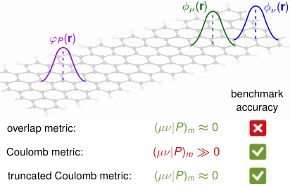
for computing the integrals in Eq. (14) and (15), where is the Dirac distribution. The overlap metric is local in the sense that the RI basis functions do not overlap with AO basis function products in Eq. (15) if there is enough distance between their centers. This leads to vanishing three-center overlap matrix elements and increasing computational efficiency due to sparsity, as illustrated in Fig. 2.
In contrast, the Coulomb metric
| (18) |
couples RI basis functions and AO basis function pairs in Eq. (15) over effectively infinite distances due to the slow polynomial decay of as illustrated in Fig. 2.Luenser et al. 2017 With the Coulomb metric, no sparsity can be gained hampering its usage in low-scaling algorithms. In canonical algorithms, each AO product is transformed to the delocalized molecular orbital basis loosing all sparsity anyway.Del Ben et al. 2013, Wilhelm et al. 2016, Rybkin and VandeVondele 2016, Ren et al. 2012, Luenser et al. 2017, Weigend et al. 1998, Gui et al. 2018, Holzer and Klopper 2019, Holzer et al. 2019, Wilhelm and Hutter 2017, Rybkin 2020, Hutter et al. 2018 In such a conventional algorithm, where sparsity cannot be exploited, the Coulomb metric is the optimal choice because the RI factorization given in Eq. (13) converges much quicker with respect to the RI basis set size.Vahtras et al. 1993 The Coulomb metric yields thus generally higher accuracy than the overlap metric.
In this work, we improve our previous low-scaling implementationWilhelm et al. 2018 by replacing the overlap metric by the truncated Coulomb metricJung et al. 2005, Jung et al. 2007, Reine et al. 2008, Luenser et al. 2017
where the Coulomb interaction is cut after a distance . In the limit of a large cutoff radius , the truncated Coulomb metric turns into the Coulomb metric, . For a small cutoff radius , calculations based on the truncated Coulomb metric are equivalent to calculations based on the overlap metric.Luenser et al. 2017 The truncated Coulomb metric combines the attractive features of the Coulomb metric and the overlap metric: high accuracy due to the near-sighted Coulomb operator and preservation of sparsity due to the locality of .
Another approach for truncating the Coulomb operator is the use of complementary error functions as in standard range-separated hybrid functionals.Heyd et al. 2003, Dutoi and Head-Gordon 2008 The benefits of a local Coulomb metric have already been exploited for low-scaling scaled-opposite spin MP2Jung et al. 2007 and low-scaling RPALuenser et al. 2017, Graf et al. 2018, Beuerle et al. 2018, Beuerle and Ochsenfeld 2018, Graf et al. 2019 reporting similar accuracy as for the respective conventional-scaling schemes.
The RI factorization in Eq. (13) is exact in the limit of a complete RI basis, independent of the chosen RI metric. Therefore, truncating the Coulomb operator with a finite does not affect the accuracy of the algorithm as long as the RI basis is sufficiently large.
We note that in plane-wave implementations, RI with different metrics is not discussed. The reason is that the Coulomb matrix, the truncated Coulomb matrix and the overlap matrix are diagonal in the plane-wave basis. As consequence, RI factorizations as in Eq. (13) are identical for the three different metrics when using plane wave basis functions. We added a more detailed explanation in the supporting information (SI) to facilitate the discussion between plane-wave and localized-basis-set communities.
3.3 Global vs. local RI
The sums over the RI basis functions in the RI factorization of the 4c Coulomb integrals in Eq. (13) can either run over the whole RI basis (”global RI”) or only over a subset of the RI basis (”local RI”). In their recent work, Förster and VisscherFörster and Visscher 2020 combined the space-time method with the pair-atomic RI (PARI) approach.Merlot et al. 2013 PARI, also known as pair-atomic density fitting (PADF) or RI-LVL,Ihrig et al. 2015 is a local RI approach, which employs the Coulomb metric. Locality is introduced by expanding each AO pair , where is centered at atom and at atom , only in the subset of RI basis functions with centers at and .
The scaling with PARI is the same as with global RI, if a local RI metric (overlap, truncated Coulomb) is employed for the latter. However, PARI reduces the computational prefactor dramatically compared to global RI since the number of three-center integrals is substantially smaller. For example, the computational cost of a calculation on 400 atoms with around 8000 AOs is 4000 CPU hours with our low-scaling scheme using global RI with the overlap metric,Wilhelm et al. 2018 but only 200 CPU hours with the PARI implementation by Förster and Visscher.Förster and Visscher 2020 However, reaching high accuracy in low-scaling PARI- seems more challenging.Förster and Visscher 2020
The accuracy of local RI schemes can be improved by adding high-angular-momentum functions to the RI basis set and increasing its size.Ihrig et al. 2015, Ren et al. 2020 It has been recently shown for a local RI variant of a implementation with conventional scaling that good accuracy can be obtained with carefully chosen RI basis sets.Ren et al. 2020 However, local RI schemes tend to ill-conditioning problemsGolze et al. 2017 introduced by very large RI basis sets, which might limit the attainable accuracy to some extent. It should be generally easier to reach high accuracy with MADs 10 meV, which is the focus of this work, with global RI-tC rather than a local PARI-type approach.
4 GW space-time method in a Gaussian basis using RI with the truncated Coulomb metric
In the following, we present our low-scaling algorithm, which is a variant of the space-time method introduced in Section 2, and rationalize where the RI factorization from Eq. (13) enters the algorithm.
4.1 Low-scaling algorithm
The MOs are expanded in Gaussian-type orbitals (GTOs)
| (21) |
where are the MO coefficients. The single-particle Green’s function given in Eq. 2 is then projected in the GTO basis
| (22) | ||||
Next, we use and Eq. (3), , to obtain the irreducible polarizability in the Gaussian auxiliary basis Wilhelm et al. 2016, Weigend et al. 1998, Del Ben et al. 2013, Pritchard et al. 2019
| (23) |
The three-center integrals are defined in Eq. (15) and originate from the RI factorization of the 4c-CIs given in Eq. (13). The expression for in Eq. (23) is generic for any RI metric . The evaluation of is the computationally most expensive step and scales with the conventional Coulomb metric (Eq. (18)). However, when employing a local RI metric, the three-center tensors vanish unless the Gaussian functions , and are centered on nearby atoms, which is illustrated in Fig. 2. In this work, we use the local truncated Coulomb metric defined in Eq. (3.2). The computational complexity for the evaluation of reduces with a local metric to .
A detailed analysis of the computational complexity of Eq. (23) is shown in Fig. 3. First, the multiplication of the three-center integrals with the Green’s function is computed, which yields the tensors and . The evaluation of and scales cubically with a nonlocal metric, but only quadratically with a local metric. The subsequent tensor contraction of and is a step of complexity with a nonlocal metric, which is reduced to with the local variant. The scaling behavior in Fig. 3 (b) can be understood as follows: For computing a single matrix element with a local metric, only a small -scaling number of indices (spatially close to ) and indices (spatially close to ) need to be taken into account. Since the number of -pairs increases as , we end up with a final scaling of for the whole matrix .
We proceed by including the matrix elements from Eq. (14) in ,
| (24) |
The polarizability is transformed to imaginary frequency via a cosine transform and the symmetric dielectric function is computed by
| (25) |
where denotes the Cholesky decomposition of the Coulomb matrix from Eq. (16),
| (26) |
The screened Coulomb interaction is split into the bare Coulomb interaction and the correlation contribution, and the latter is obtained as
| (27) |
where the symmetric, positive definite is inverted efficiently by Cholesky decomposition.
A cosine transform converts (Eq. (27)) back to the imaginary time domain. Computing the quasiparticle energy for an orbital requires the corresponding diagonal matrix element of the self-energy,
| (28) |
Its correlation part is obtained as
| (29) |
where , and the exchange part is computed as
| (30) |
where
| (31) |
In order to compute quasiparticle energies, is transformed to imaginary frequencies by a sine and cosine transform.Liu et al. 2016 The self-energy is then evaluated on the real frequency axis by analytic continuation of .van Setten et al. 2015, Liu et al. 2016, Duchemin and Blase 2020, Wilhelm et al. 2016 The energies are obtained by solving the QP equation
| (32) |
iteratively for via Newton-Raphson.
The calculation of the polarizability in Eq. (23) remains also at complexity the computational bottleneck, even for the largest systems studied in this work. The subsequent steps in Eqs. (24) – (27) scale cubically, but have a much smaller computational prefactor. The calculation of the correlation self-energy from Eq. (29) scales as for every QP level and is generally computationally less demanding than the calculation of .
4.2 Tracing back four-center Coulomb integrals and RI factorizations
While the full derivation of the algorithm presented in Section 4.1 is too lengthy, we demonstrate in the following that the tree-center integrals integrals and the metric matrix originate indeed from the RI factorization of the 4c-CIs introduced in Eq. (13). We will rationalize that the 4c-CIs can be fully recovered with the consequence that our algorithm is exact in the limit of a complete RI basis set.
For the exchange part of the self-energy, the 4c-CIs can be directly obtained by inserting Eq. (31) into Eq. (30) and using Eq. (13), which yields the familiar expression for the exchange self-energy,Wilhelm et al. 2016 .
The RI factorization of the 4c-CIs is less obvious for the correlation part of the self-energy and the intermediate steps. We exemplarily show for the matrix elements , where the 4c-CIs occur. To this end, we use the Taylor expansion to express the inverse of the dielectric function from Eq. (25) as
| (33) |
We can then rewrite Eq. (27) as
| (34) |
After inserting Eqs. (24) and (26) into Eq. (34), we obtain
| (35) |
With Eq. (23), we recover the RI expression (13) in the quadratic term:
| (36) | ||||
| (37) |
5 Implementation details
We have implemented the low-scaling algorithm outlined in Section 4.1 in the open-source software package CP2KKühne et al. 2020 which is available from github.cp2 The parallelization of the algorithm is mostly based on the standard message passing interface (MPI). OpenMP threading in a hybrid MPI+OpenMP approach is also supported. All steps of the algorithm have been optimized for massively parallel executation on more than 10,000 CPU cores. Most optimization efforts were dedicated to the computationally most expensive step, the calculation of , using the concepts outlined in Ref. 27 and the DBCSR library for sparse matrix-tensor operations.Borštnik et al. 2014 DBCSR is also employed for sparse matrix-matrix operations in Eqs. (29), and (30).
The proper choice and optimization of the imaginary-time and imaginary-frequency grids is crucial for computational efficiency and accuracy. We employ the minimax time and frequency grids with grid points as pioneered by Kaltak et al.Kaltak et al. 2014 and Liu et al.Liu et al. 2016 For minimax, the a-priori known analytical structure of , and is used to construct grids that minimize the norm of the error between exact integration and numerical integration. Following this procedure, optimal grids can be constructed for the Fourier transformsLiu et al. 2016, Kaltak et al. 2014 of the respective functions ,
| (38) | ||||
| (39) |
For simplicity, we compute the weights and during the program execution from minimization.Kaltak et al. 2014
Minimax grids are constructed by the Remez algorithm, which requires higher numerical precision than the standard double precision used in electronic-structure calculations. The minimax grids are therefore not optimized during run-time, but computed with quadruple precision and pretabulated.Braess and Hackbusch 2005 For details on generating minimax grids, we refer to the comprehensive literature.Kaltak et al. 2014, Liu et al. 2016 Note that minimax grids were recently also developed for finite-temperature .Kaltak and Kresse 2020
In our previous work,Wilhelm et al. 2018 we employed 12 minimax points. To achieve higher accuracy, we have now computed minimax grids with 26, 28, 30, 32, and 34 points in imaginary time and imaginary frequency for different ranges.Kaltak et al. 2014 These grids are freely available on github cp2 for usage with other codes implementing the space-time method. As we demonstrate in Section 7, benchmark accuracy is already obtained with 30 minimax points. Since the convergence of the Remez algorithm is increasingly difficult with the number of points, the generation of grids with more than 34 points has not been attempted.
6 Computational details
The low-scaling calculations are performed with the program package CP2K Kühne et al. 2020 and reference calculations are carried out with the program package FHI-aims.Blum et al. 2009 The input and output files of these calculations are available from the Novel Materials Discovery (NOMAD) repository.Golze 2020
6.1 Low-scaling GW calculations using CP2K
We perform calculations with the low-scaling algorithm on the benchmark set (Section 7) and as well as ev calculations on phosphorene nanosheets (Section 8 – 10). All calculations start from all-electron DFT calculations using the Gaussian and augmented plane-waves scheme (GAPW)Lippert et al. 1999 and the Perdew-Burke-Ernzerhof (PBE)Perdew et al. 1996 exchange-correlation functional. We use the RI with the truncated Coulomb metric with a truncation radius of Å, unless otherwise noted. The self-energy is analytically continued from the imaginary to the real-frequency domain using a Padé modelVidberg and Serene 1977, van Setten et al. 2015, Liu et al. 2016 with 16 parameters.
For the benchmark calculations, we use the def2-QZVPWeigend et al. 2003 basis set as primary basis set and def2-TZVPPD-RIFITHättig 2005 as auxiliary basis set. We employ minimax grids with time and frequency minimax points for the study, unless otherwise stated.
The molecular geometries of the phosphorene nanosheets are obtained as follows: We relax the unit cell of free-standing phosphorene using PBE-D3,Perdew et al. 1996, Grimme et al. 2010 Goedecker-Teter-Hutter pseudopotentials Goedecker et al. 1996 and a TZVP-MOLOPT basis setVandeVondele and Hutter 2007 using an 8 6 -point mesh. Then, an () supercell is formed, periodic boundary conditions are removed and dangling bonds are saturated by hydrogen atoms. The hydrogen atoms are relaxed with PBE-D3 while keeping the phosphorus atoms fixed.
For the calculations on phosphorene nanosheets, we employ the all-electron aug-cc-pVDZ basis setsDunning 1989, Woon and Dunning 1994, Kendall et al. 1992 in combination with the RI basis set aug-cc-pVDZ-RIFIT. Hättig 2005, Weigend et al. 2002, Pritchard et al. 2019 The lowest exponents of the RI basis set have been scaled up for the calculations on the large phosphorene sheets reported in Section 9 to improve the performance; see SI for details. Minimax grids with 30 time and frequency points are used for the small phosphorene clusters studied in Section 8, while 14 minimax points are used for the large phosphorene sheets. In the sparse matrix-tensor operations from Eq. (23), we filter atomic tensor blocks conservatively with a Frobenius norm of the atomic blocks of . For ev, we employ 80 occupied and 80 unoccupied levels in the self-consistency loop. For levels outside this range, a constant shift in the ev cycle has been applied.
With these settings, we find that the and ev HOMO-LUMO gap of the large phosphorene sheets (Section 9) is converged within 0.02 eV compared to calculations using a fully converged minimax grid of 30 points and the aug-cc-pVQZDunning 1989, Kendall et al. 1992 basis set, see SI for more details. An extrapolation to the complete basis set limit, as often necessary in , is therefore not required. HOMO-LUMO gaps typically converge faster with respect to basis set size than ionization potentials and affinities, which was demonstrated in, e.g., Ref. 21 for subsets of medium and large molecules from the database.Stuke et al. 2020
Additionally, we compute the PBE gap of 2D periodic phosphorene from GAPW all-electron calculations using the aug-cc-pVTZ basis setDunning 1989, Woon and Dunning 1994, Kendall et al. 1992 and an 8 6 -point mesh.
6.2 Reference GW calculations with contour deformation using FHI-aims
We perform reference DFT calculations with the PBE functional for all phosphorene nanosheets and @PBE calculations for the smaller phosphorene nanosheets up to 180 atoms using the FHI-aims program package.Blum et al. 2009 FHI-aims is a native all-electron code based on numeric atomic-centered orbitals (NAOs). For direct comparison with the low-scaling calculations, we employ also the aug-cc-pVDZ Gaussian basis sets, which can be considered as a special case of an NAO and which are treated numerically in FHI-aims. The auxiliary basis sets are constructed “on-the-fly” by forming product pairs of primary basis functions and subsequent removal of linear dependencies as described in Ref. 46.
The calculations are performed with the contour deformation implementationGolze et al. 2018 in FHI-aims, unless otherwise noted. As for the low-scaling CP2K calculations, the QP equations are always solved iteratively. In addition to computing the QP energies for the phosphorene nanosheets, we also compute the self-energy matrix elements for a small phosphorene cluster with 24 atoms comparing contour deformation and analytic continuation.Ren et al. 2012 For the latter, we use the Padé approximation with 16 parameters, as in the CP2K calculations. Both methods, contour deformation and analytic continuation, require the computation of integrals over the imaginary frequency axis, for which we employ a modified Gauss-Legendre gridRen et al. 2012 with 200 grid points. For the Padé model, the same set of grid points is used to calculate .
Using the same basis set, the DFT-PBE gaps of the phosphorene sheets agree within 1 meV between CP2K and FHI-aims and the gaps within 20 meV; see Table II (SI).
7 GW100 benchmark: accuracy of frontier orbitals
In the following, we assess the accuracy of the low-scaling algorithm for HOMO and LUMO QP energies of molecules from the benchmark set.van Setten et al. 2015 We carefully study their convergence with the minimax integration grid size, the RI basis set size and the truncation radius used for the RI-tC metric.
7.1 Data set and reference values
The benchmark set contains HOMO and LUMO energies of 100 small molecules featuring a variety of elements from the periodic table. We exclude the multi-solution cases BN, BeO, MgO, O3 and CuCN from computing the MAD of the HOMOs for the following reasons. First, the real self-energy matrix elements of these molecules exhibit poles in the frequency region of the quasiparticle, leading to at least two different solutions with similar spectral weight.van Setten et al. 2015 Different codes might find equally valid solutions and one should rather compare the self-energy matrix elements, as done in Ref. 15. Second, 128 Padé parameters are necessary to resolve these poles.van Setten et al. 2015 This implies that must be computed on a frequency grid of at least 128 points, which is far beyond the size of currently available minimax grids. All 100 molecules are included for the MAD of the LUMO.
We use the @PBE results from FHI-aims reported in the original workvan Setten et al. 2015 as reference. The FHI-aims results from Ref. 15 were computed with analytical continuation using the Padé model approximation with 16 parameters, as in our approach. The analytic-continuation results from FHI-aims are of high numerical quality for frontier orbitals, matching the results from a fully analytic evaluation of the self-energy within a few meV, as shown for a subset in Ref. 15. Our goal is to assess the numerical accuracy of the algorithm for a given primary basis set. We therefore compare the data directly at the def2-QZVP level instead of basis-set extrapolated results.
7.2 Convergence of minimax grid
| MAD (eV) | MAD 0.01 eV | MAD 0.02 eV | ||||
|---|---|---|---|---|---|---|
| HOMOs | LUMOs | HOMOs | LUMOs | HOMOs | LUMOs | |
| 10 | 0.098 | 0.046 | 24 | 26 | 36 | 41 |
| 20 | 0.025 | 0.013 | 32 | 77 | 66 | 96 |
| 26 | 0.014 | 0.009 | 75 | 92 | 84 | 98 |
| 28 | 0.009 | 0.007 | 81 | 94 | 89 | 97 |
| 30 | 0.007 | 0.006 | 87 | 93 | 92 | 98 |
| 32 | 0.007 | 0.005 | 88 | 94 | 91 | 99 |
| 34 | 0.007 | 0.005 | 92 | 95 | 93 | 98 |
The convergence of the @PBE QP energies with respect to to the size of our generated minimax grids is reported in Table 1. Except for different minimax parameters, the settings given in Section 6.1 were used. The MADs with respect to the reference results decrease quickly with the grid size. Already for 28 minimax points, we observe an MAD of 10 meV for both, HOMOs and LUMOs. The accuracy saturates at 30 minimax points with an MAD of 7 meV for HOMOs and 6 meV for LUMOs. The gain of accuracy when employing even larger grids with 32 and 34 points is marginal. Therefore, we set the minimax grid with 30 point as default for benchmark studies with the low-scaling algorithm.
The low-scaling algorithm reported in Ref. 56, which is the PAW variant of the space-time method, reaches high accuracy already for smaller minimax grids. Liu et al.Liu et al. 2016 showed that 20 time and frequency points were sufficient to reach convergence within 10 meV. As shown in Table 1, the MAD is still larger than 20 meV with the same grid size in our scheme. The different convergence behaviour is probably due to the different treatment of the core electrons. The low-scaling PAW- schemes does not treat the core electrons explicitly, which reduces the minimax rangeKaltak et al. 2014 compared to our all-electron scheme. With smaller minimax ranges less grid points are generally needed to obtain the same accuracy.
7.3 Convergence of RI basis sets and truncation radius
The other two parameters, which influence the accuracy of the low-scaling algorithm, are the RI basis set size and the Coulomb cutoff radius for the RI-tC metric. Both parameters are in principle interdependent since the cutoff radius controls if the metric is more “overlap-like” or rather resembles the conventional Coulomb metric, which requires smaller RI basis set sizes as discussed in Section 3.2.
Figures 4 (a) and (b) show the MAD for the reference data as function of the RI basis set size for HOMO and LUMO, respectively. We study the RI basis set convergence for two cutoff values, Å and Å. We observe a more consistent convergence behaviour when using the larger cutoff Å. For Å, the smallest MAD (10 meV) is obtained with the def2-TZVPPD-RIFIT basis. The accuracy becomes worse for larger RI basis sets which might be related to ill-conditioning problems. The truncation at Å yields higher accuracy than Å for all RI basis sets that have been tested. The MAD is well below 10 meV for def2-TZVPPD-RIFIT and the next larger RI basis set.
In Fig. 4 (c) and (d), we employ def2-TZVPPD-RIFIT as RI basis and vary the Coulomb cutoff radius used in RI-tC. For Å, the RI metric is equivalent to the overlap metric and we obtain an MAD of 30 meV for the HOMO, which is close to the 35 meV deviation reported in our previous workWilhelm et al. 2018 for the low-scaling algorithm with the overlap metric. The accuracy improves when increasing the Coulomb cutoff radius saturating at radii Å. This observation and the rapid convergence of the RI basis set with Å in Fig. 4 (a) and (b) imply that the attractive features of the conventional Coulomb metric are already largely restored at truncation radii between 2 - 3 Å. We choose Å as safe setting for our low-scaling calculations.
7.4 Benchmark with converged settings
We now compare the results obtained with the settings given in Section 6.1, i.e., the converged settings (30 minimax points, def2-TZVPPD-RIFIT, Å) to the FHI-aims reference data. The number of molecules with a given absolute deviation from the reference data are shown in Fig. 5 (see Table I (SI) for the raw data). We find that 87 out of 95 HOMO energies and 93 out of 100 LUMO energies agree with the FHI-aims referencevan Setten et al. 2015 within 10 meV, see also Table 1. Only three excitations for the HOMO and two excitations for the LUMO differ by more than 20 meV from the reference and the maximum deviation is 50 meV.
Compared to our old implementation with the overlap metric,Wilhelm et al. 2018 the accuracy is significantly improved. The MAD is reduced from 35 meV to 7 meV for the HOMO and from 27 meV to 6 meV for the LUMO. The MAD is now in the range that was reported for the FHI-aims reference data and the fully-analytic Turbomole results (3 meV for the HOMO and 6 meV for the LUMO).van Setten et al. 2015 The RI-tC scheme and the new minimax grids also improve the reliability of the low-scaling algorithm. The number of outliers is reduced to zero. In our previous work,Wilhelm et al. 2018 we observed 9 energies with deviations 60 meV for the HOMO and 7 for the LUMO, including a couple of extreme cases with errors of 0.7 and 2.2 eV.
8 Accuracy for semi-core and unbound states
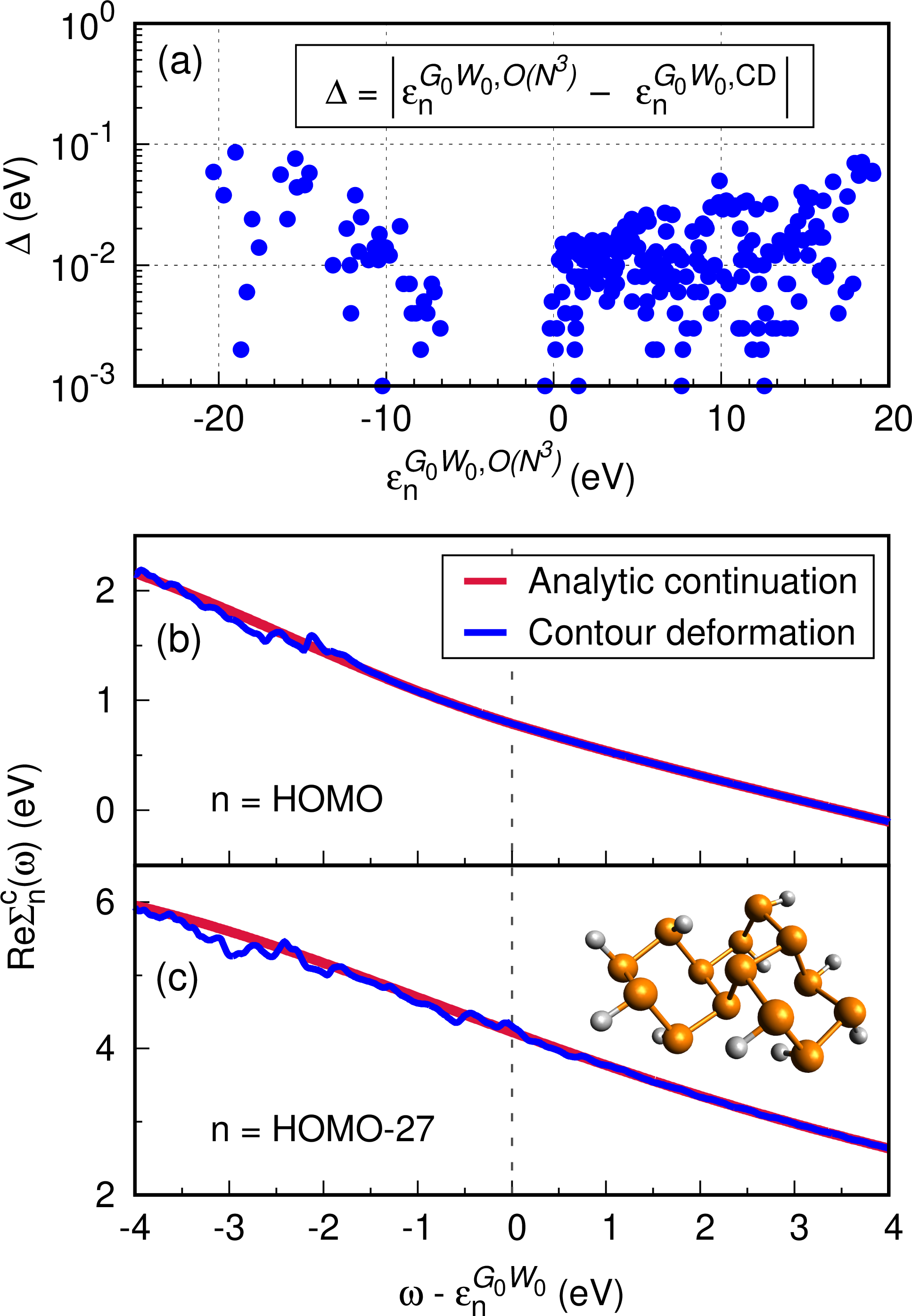
The structure of the self-energy matrix elements is typically featureless around the QP solutions for the HOMO and LUMO.van Setten et al. 2015, Golze et al. 2018, Golze et al. 2019 Achieving benchmark accuracy is thus easier for states close to the Fermi level. A more challenging test for our low-scaling algorithm are semi-core, deep valence and unbound states. In Fig. 6 (a), we report all QP energies within 20 eV distance to either HOMO or LUMO for a small phosphorene nanosheet cluster (H10P14). The cluster is shown as inlet in Fig. 6 (c) and its geometry is reported in the SI. The results are compared to QP energies computed with the highly accurate contour deformation technique (CD) implemented in FHI-aims.Golze et al. 2018 We have previously shown that the CD technique with the settings described in Section 6.2 yields without exception the same numerical accuracy as the fully analytic evaluation of the self-energy, including the difficult case of deep core states.Golze et al. 2018 By design, the CD techniques is more accurate than the analytic continuation. We set thus the CD results from FHI-aims as reference for our benchmark of semi-core and unbound states.
We find that all frontier orbitals in the frequency range HOMO2 eV and LUMO2 eV deviate by at most 0.02 eV, comparing the CD results with the energy value of the low-scaling algorithm introduced in this work, see Fig. 6 (a). The deviation increases with increasing distance from the Fermi level. However, the error is for all levels between eV and 20 eV below 0.10 eV.
The increasing deviation is attributed to the analytic continuation technique, which is employed in our low-scaling algorithm. In the final step of the algorithm, the self-energy is analytically continued to the real axis by fitting the matrix elements to a multipole model. These models are usually flexible enough to describe frontier orbitals, as shown in Fig. 6 (b). The self-energy is smooth in the frequency region of the HOMO QP energy and is perfectly reproduced by the analytic continuation around the HOMO QP energy. For deep valence and semi-core states and unbound states, increasingly acquires features around the QP energy. This is demonstrated for state HOMO-27 of the phosphorene nanosheet cluster in Fig. 6 (c). The real part of has shallow poles around , which are broadened in our CD calculation. These broadened poles appear as “ripples” in the self-energy. It is practically impossible to reproduce these small pole features with analytic continuation exactly. This is true for canonical as well as low-scaling implementations of the analytic continuation.
The acquisition of pole features around the QP energy for states far from the Fermi level is a conceptual problem of PBE. This can be best understood when rewriting the self-energy into its analytic formvan Setten et al. 2013
| (40) |
where runs over all occupied and virtual states and is a broadening parameter. are charge neutral excitations and the corresponding transition amplitudes. From Eq. (40) we directly see that the self-energy has real-valued poles (for ) at for occupied states and for virtual states. As we discussed in detail in Ref. 12, these poles give rise to satellite features, which accompany the QP excitation. The neutral excitations , which are close to eigenvalue differences, are underestimated at the PBE level. For occupied states, the PBE orbital energies are overestimated and the poles are located at too large (too positive) frequencies and are too close to the QP energy. For virtual states, the reasoning is the same, just with reverse sign, i.e., are at too small frequencies.
The problem that are located at too positive frequencies gets progressively worse for deep states, since the difference between the PBE eigenvalues and corresponding QP energies increases in absolute terms. This behaviour is visible in Fig. 6 (b) and (c) for the calculation with the exact CD technique. The shallow pole structure is for HOMO–27 in the frequency region of the QP energy, , whereas for the HOMO the shallow pole structure is located 2 eV off from the QP energy.
It has been shown that the correct distance between the poles and the QP solution can be restored in an ev scheme,Gatti et al. 2015, Zhou et al. 2015 even in the extreme case of deep core excitations.Golze et al. 2020 Since the effect of eigenvalue self-consistency in is to push the pole structure away from the QP energy,Golze et al. 2020, Golze et al. 2019 i.e., to more negative and positive frequencies for occupied and unoccupied states, respectively, the self-energy structure is also easier to model by analytic continuation for semi-core states and unbound states. We thus expect that the numerical accuracy of our low-scaling algorithm for non-frontier orbitals is even better than shown in Fig. 6 (a) when using an ev scheme.
| This work: sheet | Periodic calculation | ||||
|---|---|---|---|---|---|
| method | This work | Literature | |||
| DFT-PBE | 1.55 | 0.91 | 0.68 | 0.80 | 0.8 [112,113], 0.90 [114] |
| PBE | 3.65 | 2.13 | 1.56 | 1.60 [115], 1.83 [116], 2.0 [113], 2.03 [114], 2.06 [117] | |
| ev@PBE | 3.95 | 2.36 | 1.76 | 1.94 [118], 2.29 [114] | |
| Experiment | 2.0 [118], 2.2 [119] | ||||
9 HOMO-LUMO gap of phosphorene nanosheets from GW
We apply our low-scaling code to finite hyrogen-terminated nanosheets of phosphorene. Phosphorene consists of a single layer of black phosphorus and has been first synthesized in 2014.Liu et al. 2014, Li et al. 2014 Phosphorene forms an armchair-like vertically buckled structure of bonded phosphorus atoms, as shown in Fig. 7 (a) and (b). It has attracted vibrant research interest as two-dimensional semiconductorLing et al. 2015 because of its direct band gap of 2 eV at the point.Liang et al. 2014, Wang et al. 2015 The band gap can be successively decreased from 2 eV to 0.3 eV (3D bulk limit) by increasing the number of layers.Castellanos-Gomez 2015 This band gap range is ideal for many optoelectronic, photovoltaic and photocatalytic applications.Castellanos-Gomez 2015 DeformationVlček et al. 2019 and twisting of layers Brooks et al. 2020 have been also proposed as methods to modify the band gap of phosphorene.
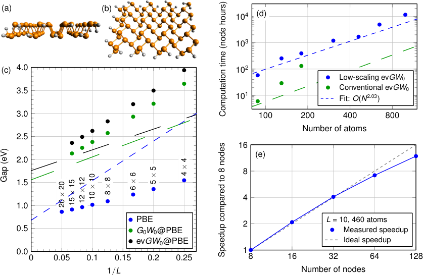
We show in this work, that the band gap can be also engineered in the in-plane direction towards values larger than 2 eV by exploiting finite size effects, which has been recently also reported from Quantum Monte Carlo calculations.Frank et al. 2019 We study here rectangular hydrogen-terminated phosphorene sheets of size , where indicates the repetition of the phosphorene unit cell, see Fig. 7 (a) and (b) for a sketch of the molecular geometry. The smallest sheet (4 4) is of size 1.8 nm 1.3 nm, while the largest (20 20) is of dimension 9.2 nm 6.7 nm. The progression of the fundamental HOMO-LUMO gaps computed from DFT-PBE eigenvalues and @PBE and ev@PBE quasiparticle energies is displayed in Fig. 7 (c). opens the too small PBE gaps, but still suffers from a starting point dependence on the underlying DFT calculation. The gaps are smaller than the ones from the partially self-consistent ev scheme, which reduces the dependence on the DFT functional. With all three methods, the computed gaps decrease with increasing sheet size; see also Table 2. At our highest level of theory, ev@PBE, the HOMO-LUMO gap changes from 3.95 eV (44) to 2.36 eV (1515). In other words, our calculations indicate that the gap of phosphorene nanosheets can be tuned by more than 1.5 eV when changing the sheet area by a factor of 14.
It is further observed that the PBE, and ev gaps follow a behaviour for the sheets; see Fig. 7 (c). The same scaling has been reported for DFT-PBE computed gaps of 1D-periodic zigzag phosphorene ribbons, whereas an has been found for the gaps of their armchair analog.Tran and Yang 2014 Our phosphorene sheets feature zigzag as well as armchair edges and we observe here, in agreement with Ref.126, the dominant scaling of the zigzag edges.
In Fig. 7 (c), we extrapolate the gaps towards the 2D bulk limit of phosphorene (). The extrapolated gaps are 0.68 eV (PBE), 1.56 eV () and 1.76 eV (ev). We are confident that our computed gaps of the finite phosphorene sheets are of high numerical quality: In Table II (SI), we show that our gaps are well converged with respect to basis set size. Additionally, we use a highly accurate full-frequency method for the self-energy evaluation, as we have demonstrated in Section 8. However, the comparison of our extrapolated gaps to gaps from periodic calculations or the experimentally measured gap of 2D periodic phosphorene (see Table 2) must be taken with a grain of salt. It has been reported in the literature that finite phosphorene sheets host edge statesPeng et al. 2014, Liang et al. 2014 that are energetically close to the band edges. These edge states are absent in 2D periodic phosphorene and hence, extrapolating the gap of finite phosphorene sheets may result in a gap that differs from the 2D periodic phosphorene gap. As first sanity check, we compare the periodic DFT-PBE gap (0.80 eV) and the DFT-PBE gap from extrapolation (0.68 eV) (see Table 2), finding a significant difference of 0.12 eV. We hypothesize that this difference also translates to such that our gap extrapolation might underestimate the actual 2D bulk limit by at least 0.1 eV.
While our cluster approach might suffer from a conceptual problem for the periodic limit (edge states), periodic calculations of 2D systems face several computational challenges as described in Ref. 128 and summarized in the following. Indicative for these numerical challenges is the relatively large spread of the reported periodic gaps of 1.6 - 2.1 eV () and 1.9 - 2.3 eV (ev); see Table 2. These variations are most likely due to insufficiencies in the numerical treatment and lack of convergence, which has been systematically studied by Qiu et al.Qiu et al. 2016 for a similar system (monolayer of MoS2). For the latter, the reported gaps varied within a similar range as for phosphorene.
One of the computational challenges in 2D-periodic calculations is the different screening parallel and perpendicular to the surface, which requires an anisotropic treatment of the singularities of at the point.Freysoldt et al. 2008 A related aspect is that the -point convergence is much slower than for three-dimensional systems, which has been also explicitly shown for phosphorene.Rasmussen et al. 2016 An additional complication is the interaction between the 2D slabs in a 3D periodic approach with plane waves. The vacuum spacing between the repeated slabs cannot be converged out due to the long-range nature of the image charge interaction between the slabs. The correct behavior can be restored by using Coulomb truncation schemesIsmail-Beigi 2006, Qiu et al. 2016 or post-processing corrections.Freysoldt et al. 2008 All these issues are avoided in our cluster approach, where periodic boundary conditions are not employed.
10 Computational efficiency
Finally, we use the phosphorene nanosheets to demonstrate the scaling and the parallel efficiency of our algorithm. As illustrated in Fig. 7 (d), the scaling is preserved from our previous work.Wilhelm et al. 2018 The largest calculations were performed for the phosphorene sheets with 990 atoms (15 15 sheet), which corresponds to 6795 electrons per spin that are expanded in 25110 basis functions. The crossover between the traditional implementation and the low-scaling calculation is at around 300 atoms [ 2100 electrons per spin, 7600 basis functions]. As shown in Fig. 7 (d), the crossover point is found by extrapolation due to the high memory demands of the conventional algorithm, which practically restricts the conventional calculations to phosphorene sheets of 200 - 250 atoms. Our low-scaling approach improves also the scaling with respect to memory consumption. The conventional implementation scales in memory, which is reduced to in this work.
In our previous implementation of low-scaling with the overlap metric, we reported a crossover point at 150 atoms for quasi-1D graphene nanoribbons.Wilhelm et al. 2018 The shift to 300 atoms is because of the larger amount of three-center integrals, that need to be included in the computation of in Eq. (23). This is caused by three circumstances. First, sparsity conditions are only met for larger system sizes due to the 2D nature of the phosphorene sheets, whereas graphene nanoribbons are quasi-1D systems. Second, we use in this work a Gaussian basis set (aug-cc-pVDZ) with much smaller exponents than in Ref. 19. The aug-cc-pVDZ basis comprises very diffuse functions (lowest Gaussian exponent in aug-cc-pVDZ for H: 0.02974 a.u., for P: 0.0343 a.u.). For diffuse functions, less three-center integral are zero than for more compact basis sets. Third, the truncated Coulomb metric is ”less local” than the overlap metric used in Ref. 19. All three points increase the computational prefactor, which is the reason, why the largest phosphorene sheet contains “only” 990 atoms, while in Ref. 19, we reported calculations of a graphene nanoribbon with around 1700 atoms.
The parallel performance of our low-scaling algorithm is assessed for the 10 10 phosphorene sheet (460 atoms) employing the cc-pVDZ basis set.Dunning 1989 Strong scaling measurements for this system are reported in Fig. 7 (e), where the speed-up of the calculation with respect to 8 computing nodes is shown. The calculation for the 10 10 sheet scales well up to 128 nodes (6144 processes) with a parallel efficiency of 74 %. Note that the calculation for the sheet runs also on 2 – 7 nodes thanks to an iterative memory reduction scheme.Wilhelm et al. 2016 This scheme overcomes memory bottlenecks for small node numbers by additional communication, without increasing the number of operations. Nevertheless, the additional MPI communication slightly increases the computational cost, which results in a better than ideal speed-up for larger node numbers, which do not require memory reduction. For a fair assessment of the parallel performance, we choose thus 8 nodes as reference in Fig. 7 (e) and the cc-pVDZ basis set instead of the aug-cc-pVDZ. The latter is more diffuse and requires more memory than cc-pVDZ, triggering the memory reduction scheme also for node numbers larger than 8.
The parallel performance and computational efficiency is also excellent for the larger phosphorene sheets. The ev calculation for the sheet (990 atoms) was performed on 768 nodes ( 37,000 CPU cores) with a run time of 15 h.
11 Conclusion
We have presented an accurate low-scaling algorithm for computing quasiparticle energies in the approximation for systems up to 1000 atoms. The algorithm achieves high accuracy by using the RI approach with the truncated Coulomb metric in combination with carefully (pre)optimized minimax grids up to 34 time and frequency points each. We have implemented the method in the open-source quantum chemistry package CP2KKühne et al. 2020 and benchmarked the accuracy for HOMOs and LUMOs using the 100 test set. The MADs with respect to the reference values from canonical implementations are 7 meV and 6 meV, respectively. The benchmark studies have been extended to semicore states and unbound unoccupied states using a 24-atom phosphorene cluster. We have shown that all quasiparticle levels in the range between HOMO-20 eV and LUMO+20 eV agree with the highly accurate contour-deformation results from FHI-aims within 0.10 eV. The reported high accuracy together with the good scalability to 1000 atoms is yet another stepping stone towards predictive calculations on nanostructured materials. We have demonstrated this on the example of phosphorene, showing that finite size effects can be used to engineer its band gap.
1012In the SI, we show that the RI factorization in a plane-wave RI basis set is independent of the RI metric. We report the results for the 100 benchmark set with 30 minimax points. We provide an input file of CP2K for the 100 test, the xyz geometry of the test of Fig. 3, the customized RI basis set for hydrogen and phosphorus and a CP2K input for a large-scale calculation. Moreover, a detailed comparison between FHI-aims and CP2K on the phosphorene sheets from Section 9 is given.
References
- Hedin [1965] Hedin, L. New Method for Calculating the One-Particle Green’s Function with Application to the Electron-Gas Problem. Phys. Rev. 1965, 139, A796–A823.
- Golze et al. [2019] Golze, D.; Dvorak, M.; Rinke, P. The Compendium: A Practical Guide to Theoretical Photoemission Spectroscopy. Front. Chem. 2019, 7, 377.
- Reining [2017] Reining, L. The approximation: content, successes and limitations. WIREs Comput. Mol. Sci. 2017, 8, e1344.
- Salpeter and Bethe [1951] Salpeter, E. E.; Bethe, H. A. A Relativistic Equation for Bound-State Problems. Phys. Rev. 1951, 84, 1232–1242.
- Onida et al. [2002] Onida, G.; Reining, L.; Rubio, A. Electronic excitations: density-functional versus many-body Green’s-function approaches. Rev. Mod. Phys. 2002, 74, 601.
- Blase et al. [2018] Blase, X.; Duchemin, I.; Jacquemin, D. The Bethe–Salpeter equation in chemistry: relations with TD-DFT, applications and challenges. Chem. Soc. Rev. 2018, 47, 1022–1043.
- Blase et al. [2020] Blase, X.; Duchemin, I.; Jacquemin, D.; Loos, P.-F. The Bethe–Salpeter Equation Formalism: From Physics to Chemistry. J. Phys. Chem. Lett. 2020, 11.
- Berger et al. [2021] Berger, J. A.; Loos, P.-F.; Romaniello, P. Potential Energy Surfaces without Unphysical Discontinuities: The Coulomb Hole Plus Screened Exchange Approach. J. Chem. Theory Comput. 2021, 17, 191–200.
- Çaylak and Baumeier [2021] Çaylak, O.; Baumeier, B. Excited-State Geometry Optimization of Small Molecules with Many-Body Green’s Functions Theory. J. Chem. Theory Comput. 2021,
- Aoki and Ohno [2018] Aoki, T.; Ohno, K. Accurate quasiparticle calculation of x-ray photoelectron spectra of solids. J. Phys.: Condens. Matter 2018, 30, 21LT01.
- Golze et al. [2018] Golze, D.; Wilhelm, J.; van Setten, M. J.; Rinke, P. Core-Level Binding Energies from : An Efficient Full-Frequency Approach within a Localized Basis. J. Chem. Theory Comput. 2018, 14, 4856–4869.
- Golze et al. [2020] Golze, D.; Keller, L.; Rinke, P. Accurate Absolute and Relative Core-Level Binding Energies from . J. Phys. Chem. Lett 2020, 11, 1840–1847.
- Keller et al. [2020] Keller, L.; Blum, V.; Rinke, P.; Golze, D. Relativistic correction scheme for core-level binding energies from . J. Chem. Phys. 2020, 153, 114110.
- Zhu and Chan [2021] Zhu, T.; Chan, G. K.-L. All-Electron Gaussian-Based for Valence and Core Excitation Energies of Periodic Systems. J. Chem. Theory Comput. 2021, DOI: 10.1021/acs.jctc.0c00704.
- van Setten et al. [2015] van Setten, M. J.; Caruso, F.; Sharifzadeh, S.; Ren, X.; Scheffler, M.; Liu, F.; Lischner, J.; Lin, L.; Deslippe, J. R.; Louie, S. G.; Yang, C.; Weigend, F.; Neaton, J. B.; Evers, F.; Rinke, P. GW100: Benchmarking for Molecular Systems. J. Chem. Theory Comput. 2015, 11, 5665–5687.
- Maggio et al. [2017] Maggio, E.; Liu, P.; van Setten, M. J.; Kresse, G. GW100: A Plane Wave Perspective for Small Molecules. J. Chem. Theory Comput. 2017, 13, 635–648.
- Gao and Chelikowsky [2019] Gao, W.; Chelikowsky, J. R. Real-Space Based Benchmark of Calculations on GW100: Effects of Semicore Orbitals and Orbital Reordering. J. Chem. Theory Comput. 2019, 15, 5299–5307.
- Govoni and Galli [2018] Govoni, M.; Galli, G. GW100: Comparison of Methods and Accuracy of Results Obtained with the WEST Code. J. Chem. Theory Comput. 2018, 14, 1895–1909.
- Wilhelm et al. [2018] Wilhelm, J.; Golze, D.; Talirz, L.; Hutter, J.; Pignedoli, C. A. Toward Calculations on Thousands of Atoms. J. Phys. Chem. Lett. 2018, 9, 306–312.
- Rangel et al. [2020] Rangel, T. et al. Reproducibility in calculations for solids. Comput. Phys. Commun. 2020, 255, 107242.
- Förster and Visscher [2020] Förster, A.; Visscher, L. Low-Order Scaling by Pair Atomic Density Fitting. J. Chem. Theory Comput. 2020, 16, 7381–7399.
- Gao and Chelikowsky [2020] Gao, W.; Chelikowsky, J. R. Accelerating Time-Dependent Density Functional Theory and GW Calculations for Molecules and Nanoclusters with Symmetry Adapted Interpolative Separable Density Fitting. J. Chem. Theory Comput. 2020, 16, 2216–2223.
- Del Ben et al. [2019] Del Ben, M.; da Jornada, F. H.; Canning, A.; Wichmann, N.; Raman, K.; Sasanka, R.; Yang, C.; Louie, S. G.; Deslippe, J. Large-scale GW calculations on pre-exascale HPC systems. Comput. Phys. Commun. 2019, 235, 187–195.
- Neuhauser et al. [2014] Neuhauser, D.; Gao, Y.; Arntsen, C.; Karshenas, C.; Rabani, E.; Baer, R. Breaking the Theoretical Scaling Limit for Predicting Quasiparticle Energies: The Stochastic Approach. Phys. Rev. Lett. 2014, 113, 076402.
- Wilhelm et al. [2016] Wilhelm, J.; Del Ben, M.; Hutter, J. in the Gaussian and Plane Waves Scheme with Application to Linear Acenes. J. Chem. Theory Comput. 2016, 12, 3623–3635.
- Stuke et al. [2020] Stuke, A.; Kunkel, C.; Golze, D.; Todorović, M.; Margraf, J. T.; Reuter, K.; Rinke, P.; Oberhofer, H. Atomic structures and orbital energies of 61,489 crystal-forming organic molecules. Sci. Data 2020, 7, 58.
- Wilhelm et al. [2016] Wilhelm, J.; Seewald, P.; Del Ben, M.; Hutter, J. Large-Scale Cubic-Scaling Random Phase Approximation Correlation Energy Calculations Using a Gaussian Basis. J. Chem. Theory Comput. 2016, 12, 5851–5859.
- Kim et al. [2019] Kim, M.; Mandal, S.; Mikida, E.; Chandrasekar, K.; Bohm, E.; Jain, N.; Li, Q.; Kanakagiri, R.; Martyna, G. J.; Kale, L.; Ismail-Beigi, S. Scalable GW software for quasiparticle properties using OpenAtom. Comput. Phys. Commun. 2019, 244, 427–441.
- Sangalli et al. [2019] Sangalli, D. et al. Many-body perturbation theory calculations using the yambo code. J. Phys.: Condens. Matter 2019, 31, 325902.
- Del Ben et al. [2020] Del Ben, M.; Yang, C.; Li, Z.; da Jornada, F. H.; Louie, S.; Deslippe, J. Accelerating Large-Scale Excited-State GW Calculations on Leadership HPC Systems. 2020 SC20: International Conference for High Performance Computing, Networking, Storage and Analysis (SC). Los Alamitos, CA, USA, 2020; pp 36–46.
- Duchemin et al. [2016] Duchemin, I.; Jacquemin, D.; Blase, X. Combining the formalism with the polarizable continuum model: A state-specific non-equilibrium approach. J. Chem. Phys. 2016, 144, 164106.
- Li et al. [2016] Li, J.; D’Avino, G.; Duchemin, I.; Beljonne, D.; Blase, X. Combining the Many-Body Formalism with Classical Polarizable Models: Insights on the Electronic Structure of Molecular Solids. J. Phys. Chem. Lett. 2016, 7, 2814–2820.
- Li et al. [2018] Li, J.; D’Avino, G.; Duchemin, I.; Beljonne, D.; Blase, X. Accurate description of charged excitations in molecular solids from embedded many-body perturbation theory. Phys. Rev. B 2018, 97, 035108.
- Giustino et al. [2010] Giustino, F.; Cohen, M. L.; Louie, S. G. GW method with the self-consistent Sternheimer equation. Phys. Rev. B 2010, 81, 115105.
- Umari et al. [2010] Umari, P.; Stenuit, G.; Baroni, S. GW quasiparticle spectra from occupied states only. Phys. Rev. B 2010, 81, 115104.
- Lambert and Giustino [2013] Lambert, H.; Giustino, F. Ab initio Sternheimer- method for quasiparticle calculations using plane waves. Phys. Rev. B 2013, 88, 075117.
- Pham et al. [2013] Pham, T. A.; Nguyen, H.-V.; Rocca, D.; Galli, G. calculations using the spectral decomposition of the dielectric matrix: verification, validation, and comparison of methods. Phys. Rev. B 2013, 87, 155148.
- Govoni and Galli [2015] Govoni, M.; Galli, G. Large Scale GW calculations. J. Chem. Theory Comput. 2015, 11, 2680–2696.
- Schlipf et al. [2020] Schlipf, M.; Lambert, H.; Zibouche, N.; Giustino, F. SternheimerGW: A program for calculating quasiparticle band structures and spectral functions without unoccupied states. Comput. Phys. Commun. 2020, 247, 106856.
- Wilson et al. [2008] Wilson, H. F.; Gygi, F.; Galli, G. Efficient iterative method for calculations of dielectric matrices. Phys. Rev. B 2008, 78, 113303.
- Wilson et al. [2009] Wilson, H. F.; Lu, D.; Gygi, F.; Galli, G. Iterative calculations of dielectric eigenvalue spectra. Phys. Rev. B 2009, 79, 245106.
- Friedrich [2019] Friedrich, C. Tetrahedron integration method for strongly varying functions: Application to the self-energy. Phys. Rev. B 2019, 100, 075142.
- Duchemin and Blase [2020] Duchemin, I.; Blase, X. Robust Analytic-Continuation Approach to Many-Body Calculations. J. Chem. Theory Comput. 2020, 16, 1742–1756.
- Bintrim and Berkelbach [2020] Bintrim, S. J.; Berkelbach, T. C. Full-Frequency GW without Frequency. arXiv:2009.14315 2020,
- Blase et al. [2011] Blase, X.; Attaccalite, C.; Olevano, V. First-principles calculations for fullerenes, porphyrins, phtalocyanine, and other molecules of interest for organic photovoltaic applications. Phys. Rev. B 2011, 83, 115103.
- Ren et al. [2012] Ren, X.; Rinke, P.; Blum, V.; Wieferink, J.; Tkatchenko, A.; Sanfilippo, A.; Reuter, K.; Scheffler, M. Resolution-of-identity approach to Hartree-Fock, hybrid density functionals, RPA, MP2 and with numeric atom-centered orbital basis functions. New J. Phys. 2012, 14, 053020.
- van Setten et al. [2013] van Setten, M. J.; Weigend, F.; Evers, F. The -Method for Quantum Chemistry Applications: Theory and Implementation. J. Chem. Theory Comput. 2013, 9, 232–246.
- Bruneval et al. [2016] Bruneval, F.; Rangel, T.; Hamed, S. M.; Shao, M.; Yang, C.; Neaton, J. B. molgw 1: Many-body perturbation theory software for atoms, molecules, and clusters. Comp. Phys. Comm. 2016, 208, 149–161.
- Sun et al. [2020] Sun, Q. et al. Recent developments in the PySCF program package. J. Chem. Phys. 2020, 153, 024109.
- Wilhelm and Hutter [2017] Wilhelm, J.; Hutter, J. Periodic calculations in the Gaussian and plane-waves scheme. Phys. Rev. B 2017, 95, 235123.
- Ren et al. [2020] Ren, X.; Merz, F.; Jiang, H.; Yao, Y.; Rampp, M.; Lederer, H.; Blum, V.; Scheffler, M. All-electron periodic implementation with numerical atomic orbital basis functions: algorithm and benchmarks. arXiv:2011.01400 2020,
- Wilhelm et al. [2019] Wilhelm, J.; VandeVondele, J.; Rybkin, V. V. Dynamics of the Bulk Hydrated Electron from Many-Body Wave-Function Theory. Angew. Chem. Int. Ed. 2019, 58, 3890–3893.
- Iskakov et al. [2020] Iskakov, S.; Yeh, C.-N.; Gull, E.; Zgid, D. Ab initio self-energy embedding for the photoemission spectra of NiO and MnO. Phys. Rev. B 2020, 102, 085105.
- Vlček et al. [2017] Vlček, V.; Rabani, E.; Neuhauser, D.; Baer, R. Stochastic GW Calculations for Molecules. J. Chem. Theory Comput. 2017, 13, 4997–5003.
- Foerster et al. [2011] Foerster, D.; Koval, P.; Sánchez-Portal, D. An implementation of Hedin’s approximation for molecules. J. Chem. Phys. 2011, 135, 074105.
- Liu et al. [2016] Liu, P.; Kaltak, M.; Klimeš, J.; Kresse, G. Cubic scaling : Towards fast quasiparticle calculations. Phys. Rev. B 2016, 94, 165109.
- Duchemin and Blase [2019] Duchemin, I.; Blase, X. Separable resolution-of-the-identity with all-electron Gaussian bases: Application to cubic-scaling RPA. J. Chem. Phys. 2019, 150, 174120.
- Kim et al. [2020] Kim, M.; Martyna, G. J.; Ismail-Beigi, S. Complex-time shredded propagator method for large-scale calculations. Phys. Rev. B 2020, 101, 035139.
- Rojas et al. [1995] Rojas, H. N.; Godby, R. W.; Needs, R. J. Space-Time Method for Ab Initio Calculations of Self-Energies and Dielectric Response Functions of Solids. Phys. Rev. Lett. 1995, 74, 1827–1830.
- Rieger et al. [1999] Rieger, M. M.; Steinbeck, L.; White, I.; Rojas, H.; Godby, R. The space-time method for the self-energy of large systems. Comput. Phys. Commun. 1999, 117, 211–228.
- Vahtras et al. [1993] Vahtras, O.; Almlöf, J.; Feyereisen, M. Integral approximations for LCAO-SCF calculations. Chem. Phys. Lett. 1993, 213, 514.
- Duchemin et al. [2017] Duchemin, I.; Li, J.; Blase, X. Hybrid and Constrained Resolution-of-Identity Techniques for Coulomb Integrals. J. Chem. Theory Comput. 2017, 13, 1199–1208.
- Eshuis et al. [2010] Eshuis, H.; Yarkony, J.; Furche, F. Fast computation of molecular random phase approximation correlation energies using resolution of the identity and imaginary frequency integration. J. Chem. Phys. 2010, 132, 234114.
- Golze et al. [2017] Golze, D.; Benedikter, N.; Iannuzzi, M.; Wilhelm, J.; Hutter, J. Fast evaluation of solid harmonic Gaussian integrals for local resolution-of-the-identity methods and range-separated hybrid functionals. J. Chem. Phys. 2017, 146, 034105.
- Obara and Saika [1986] Obara, S.; Saika, A. Efficient recursive computation of molecular integrals over Cartesian Gaussian functions. J. Chem. Phys. 1986, 84, 3963–3974.
- Ahlrichs [2006] Ahlrichs, R. A simple algebraic derivation of the Obara–Saika scheme for general two-electron interaction potentials. Phys. Chem. Chem. Phys. 2006, 8, 3072–3077.
- Guidon [2010] Guidon, M. High performance Hartree-Fock exchange for large and condensed phase systems. Ph.D. thesis, University of Zuerich, 2010; pp 86-89; https://doi.org/10.5167/uzh-44716.
- Luenser et al. [2017] Luenser, A.; Schurkus, H. F.; Ochsenfeld, C. Vanishing-Overhead Linear-Scaling Random Phase Approximation by Cholesky Decomposition and an Attenuated Coulomb-Metric. J. Chem. Theory Comput. 2017, 13, 1647–1655.
- Del Ben et al. [2013] Del Ben, M.; Hutter, J.; VandeVondele, J. Electron Correlation in the Condensed Phase from a Resolution of Identity Approach Based on the Gaussian and Plane Waves Scheme. J. Chem. Theory Comput. 2013, 9, 2654–2671.
- Rybkin and VandeVondele [2016] Rybkin, V. V.; VandeVondele, J. Spin-Unrestricted Second-Order Møller-Plesset (MP2) Forces for the Condensed Phase: From Molecular Radicals to F-Centers in Solids. J. Chem. Theory Comput. 2016, 12, 2214–2223.
- Weigend et al. [1998] Weigend, F.; Häser, M.; Patzelt, H.; Ahlrichs, R. RI-MP2: optimized auxiliary basis sets and demonstration of efficiency. Chem. Phys. Lett. 1998, 294, 143–152.
- Gui et al. [2018] Gui, X.; Holzer, C.; Klopper, W. Accuracy Assessment of Starting Points for Calculating Molecular Excitation Energies Using the Bethe–Salpeter Formalism. J. Chem. Theory Comput. 2018, 14, 2127–2136.
- Holzer and Klopper [2019] Holzer, C.; Klopper, W. Ionized, electron-attached, and excited states of molecular systems with spin–orbit coupling: Two-component and Bethe–Salpeter implementations. J. Chem. Phys. 2019, 150, 204116.
- Holzer et al. [2019] Holzer, C.; Teale, A. M.; Hampe, F.; Stopkowicz, S.; Helgaker, T.; Klopper, W. quasiparticle energies of atoms in strong magnetic fields. J. Chem. Phys. 2019, 150, 214112.
- Rybkin [2020] Rybkin, V. V. Sampling Potential Energy Surfaces in the Condensed Phase with Many-Body Electronic Structure Methods. Chem. Eur. J. 2020, 26, 362–368.
- Hutter et al. [2018] Hutter, J.; Wilhelm, J.; Rybkin, V. V.; Del Ben, M.; VandeVondele, J. In Handbook of Materials Modeling: Methods: Theory and Modeling, Chapter: MP2- and RPA-Based Ab Initio Molecular Dynamics and Monte Carlo Sampling; Andreoni, W., Yip, S., Eds.; Springer, 2018.
- Jung et al. [2005] Jung, Y.; Sodt, A.; Gill, P. M.; Head-Gordon, M. Auxiliary basis expansions for large-scale electronic structure calculations. Proc. Natl. Acad. Sci. U.S.A. 2005, 102, 6692–6697.
- Jung et al. [2007] Jung, Y.; Shao, Y.; Head-Gordon, M. Fast evaluation of scaled opposite spin second-order Møller–Plesset correlation energies using auxiliary basis expansions and exploiting sparsity. J. Comput. Chem. 2007, 28, 1953–1964.
- Reine et al. [2008] Reine, S.; Tellgren, E.; Krapp, A.; Kjærgaard, T.; Helgaker, T.; Jansik, B.; Høst, S.; Salek, P. Variational and robust density fitting of four-center two-electron integrals in local metrics. J. Chem. Phys. 2008, 129, 104101.
- Heyd et al. [2003] Heyd, J.; Scuseria, G. E.; Ernzerhof, M. Hybrid functionals based on a screened Coulomb potential. J. Chem. Phys. 2003, 118, 8207–8215.
- Dutoi and Head-Gordon [2008] Dutoi, A. D.; Head-Gordon, M. A Study of the Effect of Attenuation Curvature on Molecular Correlation Energies by Introducing an Explicit Cutoff Radius into Two-Electron Integrals. J. Phys. Chem. A 2008, 112, 2110–2119.
- Graf et al. [2018] Graf, D.; Beuerle, M.; Schurkus, H. F.; Luenser, A.; Savasci, G.; Ochsenfeld, C. Accurate and Efficient Parallel Implementation of an Effective Linear-Scaling Direct Random Phase Approximation Method. J. Chem. Theory Comput. 2018, 14, 2505–2515.
- Beuerle et al. [2018] Beuerle, M.; Graf, D.; Schurkus, H. F.; Ochsenfeld, C. Efficient calculation of beyond RPA correlation energies in the dielectric matrix formalism. J. Chem. Phys. 2018, 148, 204104.
- Beuerle and Ochsenfeld [2018] Beuerle, M.; Ochsenfeld, C. Low-scaling analytical gradients for the direct random phase approximation using an atomic orbital formalism. J. Chem. Phys. 2018, 149, 244111.
- Graf et al. [2019] Graf, D.; Beuerle, M.; Ochsenfeld, C. Low-Scaling Self-Consistent Minimization of a Density Matrix Based Random Phase Approximation Method in the Atomic Orbital Space. J. Chem. Theory Comput. 2019, 15, 4468–4477.
- Merlot et al. [2013] Merlot, P.; Kjærgaard, T.; Helgaker, T.; Lindh, R.; Aquilante, F.; Reine, S.; Pedersen, T. B. Attractive electron–electron interactions within robust local fitting approximations. J. Comput. Chem. 2013, 34, 1486–1496.
- Ihrig et al. [2015] Ihrig, A. C.; Wieferink, J.; Zhang, I. Y.; Ropo, M.; Ren, X.; Rinke, P.; Scheffler, M.; Blum, V. Accurate localized resolution of identity approach for linear-scaling hybrid density functionals and for many-body perturbation theory. New J. Phys. 2015, 17, 093020.
- Golze et al. [2017] Golze, D.; Iannuzzi, M.; Hutter, J. Local Fitting of the Kohn–Sham Density in a Gaussian and Plane Waves Scheme for Large-Scale Density Functional Theory Simulations. J. Chem. Theory Comput. 2017, 13, 2202–2214.
- Pritchard et al. [2019] Pritchard, B. P.; Altarawy, D.; Didier, B.; Gibson, T. D.; Windus, T. L. New Basis Set Exchange: An Open, Up-to-Date Resource for the Molecular Sciences Community. J. Chem. Inf. Model. 2019, 59, 4814–4820.
- Kühne et al. [2020] Kühne, T. D. et al. CP2K: An electronic structure and molecular dynamics software package - Quickstep: Efficient and accurate electronic structure calculations. J. Chem. Phys. 2020, 152, 194103.
- [91] CP2K github repository, https://github.com/cp2k/cp2k (accessed December, 2020).
- Borštnik et al. [2014] Borštnik, U.; VandeVondele, J.; Weber, V.; Hutter, J. Sparse matrix multiplication: The distributed block-compressed sparse row library. Parallel Comput. 2014, 40, 47–58.
- Kaltak et al. [2014] Kaltak, M.; Klimeš, J.; Kresse, G. Low Scaling Algorithms for the Random Phase Approximation: Imaginary Time and Laplace Transforms. J. Chem. Theory Comput. 2014, 10, 2498–2507.
- Braess and Hackbusch [2005] Braess, D.; Hackbusch, W. Approximation of 1/x by exponential sums in [1,). SIAM J. Numer. Anal. 2005, 25, 685–697.
- Kaltak and Kresse [2020] Kaltak, M.; Kresse, G. Minimax isometry method: A compressive sensing approach for Matsubara summation in many-body perturbation theory. Phys. Rev. B 2020, 101, 205145.
- Blum et al. [2009] Blum, V.; Gehrke, R.; Hanke, F.; Havu, P.; Havu, V.; Ren, X.; Reuter, K.; Scheffler, M. Ab initio molecular simulations with numeric atom-centered orbitals. Comput. Phys. Commun. 2009, 180, 2175–2196.
- Golze [2020] Golze, D. Dataset in NOMAD repository “Low-scaling GW: GW100 and phosphorene”. 2020; https://dx.doi.org/10.17172/NOMAD/2021.01.15-1.
- Lippert et al. [1999] Lippert, G.; Hutter, J.; Parrinello, M. The Gaussian and augmented-plane-wave density functional method for ab initio molecular dynamics simulations. Theor. Chem. Acc. 1999, 103, 124–140.
- Perdew et al. [1996] Perdew, J. P.; Burke, K.; Ernzerhof, M. Generalized Gradient Approximation Made Simple. Phys. Rev. Lett. 1996, 77, 3865–3868.
- Vidberg and Serene [1977] Vidberg, H. J.; Serene, J. W. Solving the Eliashberg equations by means of N-point Padé approximants. J. Low Temp. Phys. 1977, 29, 179–192.
- Weigend et al. [2003] Weigend, F.; Furche, F.; Ahlrichs, R. Gaussian basis sets of quadruple zeta valence quality for atoms H–Kr. J. Chem. Phys. 2003, 119, 12753–12762.
- Hättig [2005] Hättig, C. Optimization of auxiliary basis sets for RI-MP2 and RI-CC2 calculations: Core–valence and quintuple-zeta basis sets for H to Ar and QZVPP basis sets for Li to Kr. Phys. Chem. Chem. Phys. 2005, 7, 59–66.
- Grimme et al. [2010] Grimme, S.; Antony, J.; Ehrlich, S.; Krieg, H. A consistent and accurate ab initio parametrization of density functional dispersion correction (DFT-D) for the 94 elements H-Pu. J. Chem. Phys. 2010, 132, 154104.
- Goedecker et al. [1996] Goedecker, S.; Teter, M.; Hutter, J. Separable dual-space Gaussian pseudopotentials. Phys. Rev. B 1996, 54, 1703–1710.
- VandeVondele and Hutter [2007] VandeVondele, J.; Hutter, J. Gaussian basis sets for accurate calculations on molecular systems in gas and condensed phases. J. Chem. Phys. 2007, 127, 114105.
- Dunning [1989] Dunning, T. H. Gaussian basis sets for use in correlated molecular calculations. I. The atoms boron through neon and hydrogen. J. Chem. Phys. 1989, 90, 1007–1023.
- Woon and Dunning [1994] Woon, D. E.; Dunning, T. H. Gaussian basis sets for use in correlated molecular calculations. IV. Calculation of static electrical response properties. J. Chem. Phys. 1994, 100, 2975–2988.
- Kendall et al. [1992] Kendall, R. A.; Dunning, T. H.; Harrison, R. J. Electron affinities of the first‐row atoms revisited. Systematic basis sets and wave functions. J. Chem. Phys. 1992, 96, 6796–6806.
- Weigend et al. [2002] Weigend, F.; Köhn, A.; Hättig, C. Efficient use of the correlation consistent basis sets in resolution of the identity MP2 calculations. J. Chem. Phys. 2002, 116, 3175–3183.
- Gatti et al. [2015] Gatti, M.; Panaccione, G.; Reining, L. Effects of Low-Energy Excitations on Spectral Properties at Higher Binding Energy: The Metal-Insulator Transition of . Phys. Rev. Lett. 2015, 114, 116402.
- Zhou et al. [2015] Zhou, J. S.; Kas, J. J.; Sponza, L.; Reshetnyak, I.; Guzzo, M.; Giorgetti, C.; Gatti, M.; Sottile, F.; Rehr, J. J.; Reining, L. Dynamical effects in electron spectroscopy. J. Chem. Phys. 2015, 143, 184109.
- Frank et al. [2019] Frank, T.; Derian, R.; Tokár, K.; Mitas, L.; Fabian, J.; Štich, I. Many-Body Quantum Monte Carlo Study of 2D Materials: Cohesion and Band Gap in Single-Layer Phosphorene. Phys. Rev. X 2019, 9, 011018.
- Tran et al. [2014] Tran, V.; Soklaski, R.; Liang, Y.; Yang, L. Layer-controlled band gap and anisotropic excitons in few-layer black phosphorus. Phys. Rev. B 2014, 89, 235319.
- Rasmussen et al. [2016] Rasmussen, F. A.; Schmidt, P. S.; Winther, K. T.; Thygesen, K. S. Efficient many-body calculations for two-dimensional materials using exact limits for the screened potential: Band gaps of MoS-BN, and phosphorene. Phys. Rev. B 2016, 94, 155406.
- Rudenko and Katsnelson [2014] Rudenko, A. N.; Katsnelson, M. I. Quasiparticle band structure and tight-binding model for single- and bilayer black phosphorus. Phys. Rev. B 2014, 89, 201408.
- Jiang et al. [2017] Jiang, Z.; Liu, Z.; Li, Y.; Duan, W. Scaling Universality between Band Gap and Exciton Binding Energy of Two-Dimensional Semiconductors. Phys. Rev. Lett. 2017, 118, 266401.
- Ferreira and Ribeiro [2017] Ferreira, F.; Ribeiro, R. M. Improvements in the and Bethe-Salpeter-equation calculations on phosphorene. Phys. Rev. B 2017, 96, 115431.
- Liang et al. [2014] Liang, L.; Wang, J.; Lin, W.; Sumpter, B. G.; Meunier, V.; Pan, M. Electronic Bandgap and Edge Reconstruction in Phosphorene Materials. Nano Lett. 2014, 14, 6400–6406.
- Wang et al. [2015] Wang, X.; Jones, A. M.; Seyler, K. L.; Tran, V.; Jia, Y.; Zhao, H.; Wang, H.; Yang, L.; Xu, X.; Xia, F. Highly anisotropic and robust excitons in monolayer black phosphorus. Nat. Nanotechnol. 2015, 10, 517–521.
- Liu et al. [2014] Liu, H.; Neal, A. T.; Zhu, Z.; Luo, Z.; Xu, X.; Tománek, D.; Ye, P. D. Phosphorene: An Unexplored 2D Semiconductor with a High Hole Mobility. ACS Nano 2014, 8, 4033–4041.
- Li et al. [2014] Li, L.; Yu, Y.; Ye, G. J.; Ge, Q.; Ou, X.; Wu, H.; Feng, D.; Chen, X. H.; Zhang, Y. Black phosphorus field-effect transistors. Nat. Nanotechnol. 2014, 9, 372–377.
- Ling et al. [2015] Ling, X.; Wang, H.; Huang, S.; Xia, F.; Dresselhaus, M. S. The renaissance of black phosphorus. Proc. Natl. Acad. Sci. 2015, 112, 4523–4530.
- Castellanos-Gomez [2015] Castellanos-Gomez, A. Black Phosphorus: Narrow Gap, Wide Applications. J. Phys. Chem. Lett. 2015, 6, 4280–4291.
- Vlček et al. [2019] Vlček, V.; Rabani, E.; Baer, R.; Neuhauser, D. Nonmonotonic band gap evolution in bent phosphorene nanosheets. Phys. Rev. Materials 2019, 3, 064601.
- Brooks et al. [2020] Brooks, J.; Weng, G.; Taylor, S.; Vlček, V. Stochastic many-body perturbation theory for Moiré states in twisted bilayer phosphorene. J. Phys. Condens. Matter 2020, 32, 234001.
- Tran and Yang [2014] Tran, V.; Yang, L. Scaling laws for the band gap and optical response of phosphorene nanoribbons. Phys. Rev. B 2014, 89, 245407.
- Peng et al. [2014] Peng, X.; Copple, A.; Wei, Q. Edge effects on the electronic properties of phosphorene nanoribbons. J. Appl. Phys. 2014, 116, 144301.
- Freysoldt et al. [2008] Freysoldt, C.; Eggert, P.; Rinke, P.; Schindlmayr, A.; Scheffler, M. Screening in two dimensions: calculations for surfaces and thin films using the repeated-slab approach. Phys. Rev. B 2008, 77, 235428.
- Qiu et al. [2016] Qiu, D. Y.; da Jornada, F. H.; Louie, S. G. Screening and many-body effects in two-dimensional crystals: Monolayer . Phys. Rev. B 2016, 93, 235435.
- Ismail-Beigi [2006] Ismail-Beigi, S. Truncation of periodic image interactions for confined systems. Phys. Rev. B 2006, 73, 233103.