跳到论文正文
W Papers独立论文阅读器 arXiv:2012.06244 论文正文 计算阅读时间 · 0%
引用这篇论文根据当前论文元数据生成,正式投稿前建议核对。


License: CC BY 4.0
arXiv:2012.06244v4 [cs.LG] 16 Dec 2021

The Implicit Regularization for Adaptive Optimization Algorithms on Homogeneous Neural Networks

Bohan Wang Affiliation:  Microsoft Research Asia, Beijing, China    Qi Meng Affiliation:  Microsoft Research Asia, Beijing, China    Wei Chen Affiliation:  Microsoft Research Asia, Beijing, China Correspondence to: wche@microsoft.com    Tie-Yan Liu Affiliation:  Microsoft Research Asia, Beijing, China
Abstract

Despite their overwhelming capacity to overfit, deep neural networks trained by specific optimization algorithms tend to generalize well to unseen data. Recently, researchers explained it by investigating the implicit regularization effect of optimization algorithms. A remarkable progress is the work (Lyu & Li 2019), which proves gradient descent (GD) maximizes the margin of homogeneous deep neural networks. Except GD, adaptive algorithms such as AdaGrad, RMSProp and Adam are popular owing to their rapid training process. However, theoretical guarantee for the generalization of adaptive optimization algorithms is still lacking. In this paper, we study the implicit regularization of adaptive optimization algorithms when they are optimizing the logistic loss on homogeneous deep neural networks. We prove that adaptive algorithms that adopt exponential moving average strategy in conditioner (such as Adam and RMSProp) can maximize the margin of the neural network, while AdaGrad that directly sums historical squared gradients in conditioner can not. It indicates superiority on generalization of exponential moving average strategy in the design of the conditioner. Technically, we provide a unified framework to analyze convergent direction of adaptive optimization algorithms by constructing novel adaptive gradient flow and surrogate margin. Our experiments can well support the theoretical findings on convergent direction of adaptive optimization algorithms.

Keywords: 
Adaptive Optimizer, Implicit Regularization, Margin

1 Introduction

Deep learning techniques have been very successful in several domains, like computer vision (Voulodimos et al. 2018), speech recognition (Deng et al. 2013) and natural language processing (Young et al. 2018). In practice, deep neural networks (DNN) learned by optimization algorithms such as gradient descent (GD) and its variants can generalize well to unseen data (Witten & Frank 2005). However, deep neural networks are non-convex. The non-convex deep neural networks have been found to have large amount of global minima (Choromanska et al. 2015), while only few of them can guarantee satisfactory generalization property (Brutzkus et al. 2018). Explaining why the highly non-convex model trained by a specific algorithm can generalize has become an important open question in deep learning.

Regarding the above question, one plausible explanation is that optimization algorithms implicitly regularize the training process (Neyshabur et al. 2015). That is, the optimization algorithm tends to drive parameters to certain kinds of global minima which generalize well, although no explicit regularization is enforced. Recently, exciting results have been shown for vanilla gradient descent. A remarkable progress is the work (Lyu & Li 2019), which proves that GD maximizes the margin of homogeneous (non-linear) deep neural networks.

On the other hand, adaptive algorithms such as AdaGrad (Duchi et al. 2011), RMSProp (Hinton et al. 2012), and Adam (Kingma & Ba 2015) have been in spotlight these years. These algorithms are proposed to improve the convergence rate of GD (or SGD) by using second-order moments of historical gradients as conditioner and have been widely applied in deep learning (Ruder 2016). Despite the rapid convergence of adaptive methods, numerous works have provided empirical evidence that adaptive methods may suffer from poor generalization performance (Wilson et al. 2017; Luo et al. 2018). Several works try to improve the performance of adaptive optimization algorithms such as AdamW (Loshchilov & Hutter 2018), AdaBound (Luo et al. 2018), AdaBelief (Zhuang et al. 2020). However, there is little theoretical analysis for generalization of adaptive algorithms. These observations and the research for GD motivate us to study the implicit regularization for adaptive algorithms.

The key factor for the success of adaptive optimization algorithms is to design better conditioners of the gradient. Adagrad adopts the simple average of the squared values of the historical gradients in its conditioner, while RMSProp and Adam improve the simple average to exponential moving average strategy. In this paper, we aim to study the influence of different types of conditioners on convergent direction of parameters trained by adaptive optimization algorithms. Specifically, we work on the homogeneous neural networks (including fully connected or convolutional neural network with ReLU or leaky ReLU activations) with separable data under logistic loss (for binary classification) and cross-entropy (for multi-class classification). For logistic loss, we focus on characterizing the convergent direction of parameters (i.e., limt→∞wt‖wt‖2\lim_{t\rightarrow\infty}\frac{w_{t}}{\|w_{t}\|_{2}}) with respect to the training iteration tt, which is a key target along this line of researches (Soudry et al. 2018; Gunasekar et al. 2018b; Lyu & Li 2019).

Our main result is summarized in Theorem 1, which states that RMSProp and Adam (w/m) (a variant of Adam without momentum acceleration)11 1 How momentum influence the convergence of an optimization algorithm on non-convex deep neural network is still an open problem. Here, we only study a variant of Adam which sets the momentum parameter as 00. maximize margin of the neural network (equivalent to the optimum of optimization problem in Eq.(2)) and AdaGrad does not converge to max-margin solution due to the anisotropic 𝒉∞\boldsymbol{h}_{\infty}.

Theorem 1.

(Informal) We use Φ⁡(𝐰,𝐱)\Phi(\boldsymbol{w},\boldsymbol{x}) to denote the homogeneous neural network model with parameter 𝐰\boldsymbol{w} and input 𝐱\boldsymbol{x}. (1) For AdaGrad, any limit point of wt/‖wt‖2w_{t}/\|w_{t}\|_{2} is a KKT point of the optimization problem

min∥𝒉∞−1/2⊙𝒘∥2subject to yiΦ(𝒘,𝒙i)≥1,∀i,\displaystyle\min\|\boldsymbol{h}^{-1/2}_{\infty}\odot\boldsymbol{w}\|^{2}\quad\textit{subject to }y_{i}\Phi(\boldsymbol{w},\boldsymbol{x}_{i})\geq 1,\forall i, (1)

where 𝐡∞=limt→∞𝐡⁡(t)\boldsymbol{h}_{\infty}=\lim_{t\rightarrow\infty}\boldsymbol{h}(t) is the limit of the conditioner in AdaGrad. (2) For Adam (w/m) and RMSProp, any limit point of 𝐰⁡(t)/‖𝐰⁡(t)‖2\boldsymbol{w}(t)/\|\boldsymbol{w}(t)\|_{2} is a KKT point of the optimization problem

min⁡‖𝒘‖2subject to ​yi​Φ​(𝒘,𝒙i)≥1,∀i.\displaystyle\min\|\boldsymbol{w}\|^{2}\quad\textit{subject to }y_{i}\Phi(\boldsymbol{w},\boldsymbol{x}_{i})\geq 1,\forall i. (2)

Theorem 1 indicates the importance of proper design on the conditioner, i.e., adaptive algorithms like Adam (w/m) and RMSProp that adopt exponential weighted average design on conditioner regularize the training to max-margin solution, which has low complexity. Therefore, we can expect good generalization performance for Adam (w/m) and RMSProp. Furthermore, we illustrate that the convergence direction of AdaGrad is sensitive to initialization, which hurts its generalization.

We establish Theorem 1 for both continuous flows of adaptive optimization algorithms and their discrete update rules. The technical contributions to prove Theorem 1 are summarized as follows. (1) We propose adaptive gradient flow, which is a unified framework to deal with adaptive gradients. With the adaptive gradient flow, the analysis of convergent direction is transformed from original parameter space to a normalized parameter space. (2) In the normalized parameter space, we construct surrogate margin for the adaptive algorithms, and with the surrogate margin, we show that the increasing rate of the parameter norm can be bounded by the decreasing rate of logarithmic loss and the loss converges to zero. (3) We prove that any limit direction of the normalized parameter flow is a KKT point of the margin maximization problem in normalized parameter space. Moreover, we prove the convergent direction is unique if the neural network is definable (Kurdyka 1998). The adaptive gradient flow and surrogate margin are designed for adaptive optimization algorithms, which makes the proof techniques different from that for vanilla GD in (Soudry et al. 2018; Lyu & Li 2019). (4) We further prove the convergent direction for discrete update rules by characterizing the influence of the learning rate.

Finally, we conduct experiments to observe the margin of homogeneous neural network during training of several adaptive optimization algorithms. For all experiments, the margins are increasing during training and the final margins of RMSProp and Adam (w/m) are larger than that of AdaGrad. We also observe the convergent direction of adaptive optimization algorithms under different realizations of initialization and results show that the convergent direction of AdaGrad is sensitive to initialization. These observations can well support our theoretical findings.

2 Related Work

Implicit Regularization of First-order Optimization Methods. Soudry et al. 2018 proved that gradient descent on linear logistic regression with separable data converges in the direction of the max L2L^{2} margin solution of the corresponding hard-margin Support Vector Machine, and motivate a line of works on the implicit regularization of GD on linear model (Nacson et al. 2019b; Ji & Telgarsky 2019; Li et al. 2019; Xu et al. 2018).

Afterwards, researchers study the implicit regularization of GD on deep neural networks. Ji & Telgarsky 2018; Gunasekar et al. 2018b studied the deep linear network and Soudry et al. 2018 studied the two-layer neural network with ReLU activation. Nacson et al. 2019a proved the asymptotic direction is along a KKT point of the L2L^{2} max-margin problem for homogeneous deep neural networks. Lyu & Li 2019 independently proved similar result for homogeneous neural networks with simplified assumptions. Based on (Lyu & Li 2019), Ji & Telgarsky 2020 further prove that parameters have only one asymptotic direction.

There are also works considering implicit regularization of other first-order optimization algorithms. Nacson et al. 2019c worked on Stochastic Gradient Descent for linear logistic regression. Gunasekar et al. 2018a studied mirror descent and steepest descent on linear model. Arora et al. 2019 proved gradient descent on Neural Tangent Kernel will converge to a global minimum near the initial point.

However, there is little result on the implicit regularization of adaptive optimization methods.

Theoretical Evidence of Generalization of Adaptive Algorithms. Adaptive algorithms have been in spotlight these years and many works empirically observe the generalization behavior of adaptive algorithms (Keskar & Socher 2017; Reddi et al. 2018; Chen et al. 2018; Luo et al. 2018). In comparison, there are few theoretical justifications. Wilson et al. 2017 constructed a specific linear regression task where adaptive optimization algorithms converge to a solution that incorrectly classifies new data with probability arbitrarily close to half. Zhou et al. 2020 modeled the distribution of stochastic noise in Adam, and showed that SGD tends to converge to flatter local minima. Another viewpoint is to study the convergent direction of adaptive optimization algorithms. To the best of our knowledge, the only work is (Qian & Qian 2019), which proves the convergent direction of AdaGrad on linear logistic regression. In this paper, we study the convergent direction of adaptive optimization algorithms on deep neural networks which requires different techniques due to the non-convexity of deep networks.

Meanwhile, the correlation between margin and generalization error has also been extended to deep networks. Bartlett et al. 2017 first bound the generalization error of deep neural networks using (spectrally) normalized margin by covering number. In parallel, Neyshabur et al. 2018 adopt normalized margin into the PAC-Bayesian framework and derive generalization bound with different dependency on layer width from (Bartlett et al. 2017). Empirically, Jiang et al. 2019 present a large scale study of different generalization bounds in deep networks, and find there is a significant correlation between generalization error and normalized margin when optimizer is changed. These work support our study on generalization in deep learning through the margin theory.

3 Preliminaries

In this paper, we study the logistic regression problem with homogeneous neural networks. Let training set 𝑺\boldsymbol{S} defined as 𝑺={(𝒙i,yi)}i=1N\boldsymbol{S}=\{(\boldsymbol{x}_{i},y_{i})\}_{i=1}^{N}, where 𝒙i∈𝒳\boldsymbol{x}_{i}\in\mathcal{X} (i=1,2,⋯,Ni=1,2,\cdots,N) are inputs, yi∈ℝy_{i}\in\mathbb{R} (i=1,2,⋯,Ni=1,2,\cdots,N) are labels, and NN is the size of 𝑺\boldsymbol{S}. The empirical loss ℒ\mathcal{L} with training set 𝑺\boldsymbol{S}, neural network classifier Φ\Phi, individual loss ℓ⁡(x)=e−f⁡(x)\ell(x)=e^{-f(x)} and parameters 𝒘∈ℝp\boldsymbol{w}\in\mathbb{R}^{p} can be written as follows:

ℒ⁡(𝒘,𝑺)=∑i=1Nℓ⁡(yi​Φ​(𝒘,𝒙i)).\mathcal{L}(\boldsymbol{w},\boldsymbol{S})=\sum_{i=1}^{N}\ell\left(y_{i}\Phi(\boldsymbol{w},\boldsymbol{x}_{i})\right).

In an optimization process, the training set 𝑺\boldsymbol{S} is fixed. Therefore, without loss of generality, we abbreviate ℒ⁡(𝒘,𝑺)=ℒ⁡(𝒘)\mathcal{L}(\boldsymbol{w},\boldsymbol{S})=\mathcal{L}(\boldsymbol{w}), and yi​Φ​(𝒘,𝒙i)=qi​(𝒘)y_{i}\Phi(\boldsymbol{w},\boldsymbol{x}_{i})=q_{i}(\boldsymbol{w}). In this paper, we consider the exponential loss, i.e., f⁡(qi​(𝒘))=qi​(𝒘)f(q_{i}(\boldsymbol{w}))=q_{i}(\boldsymbol{w}), and the logistic loss, i.e., f⁡(qi​(𝒘))=−log⁡log⁡(1+e−qi​(𝒘))f(q_{i}(\boldsymbol{w}))=-\log\log(1+e^{-q_{i}(\boldsymbol{w})}). Both of ff are monotonously increasing and have an inverse.

We will use Clarke’s Subdifferential ∂\partial (Clarke 1975) in this paper as a natural extension of gradient ∇\nabla for locally Lipschitz functions. For any locally Lipschitz function f:ℝp→ℝf:\mathbb{R}^{p}\rightarrow\mathbb{R}, its Clarke’s Subdifferential ∂f\partial f at point 𝒘0\boldsymbol{w}_{0} is defined as

conv{limk→∞∇f(𝒘k):𝒘k→𝒘0,∇f(𝒘k) exists }.\operatorname{conv}\{\lim_{k\rightarrow\infty}\nabla f\left(\boldsymbol{w}_{k}\right):\boldsymbol{w}_{k}\rightarrow\boldsymbol{w}_{0},\nabla f(\boldsymbol{w}_{k})\text{ exists }\}.

Following (Davis et al. 2020), we also define ff admits a chain rule if for any arc 22 2 A arc 𝒛:ℝ+→ℝp\boldsymbol{z}:\mathbb{R}^{+}\rightarrow\mathbb{R}^{p} satisfies for any compact set I⊂ℝ+I\subset\mathbb{R}^{+}, 𝒛\boldsymbol{z} is absolute continuous on II. 𝒛:ℝ+→ℝp\boldsymbol{z}:\mathbb{R}^{+}\rightarrow\mathbb{R}^{p}, ∀𝒉∈∂f⁡(𝒛⁡(t))\forall\boldsymbol{h}\in\partial f(\boldsymbol{z}(t)), d​f​(z⁡(t))d​t=⟨𝒉,d​zd​t⟩\frac{\mathrm{d}f(z(t))}{\mathrm{d}t}=\langle\boldsymbol{h},\frac{\mathrm{d}z}{\mathrm{d}t}\rangle, a.e. for t>0t>0.

3.1 Continuous Flow for Adaptive Algorithms

Adaptive optimization algorithms including AdaGrad, RMSProp, Adam are widely used to optimize the loss function in deep learning. The update rules for these adaptive optimization algorithms can be written as 33 3 In this paper, we only consider no-momentum versions of the algorithms, i.e., the algorithms without momentum acceleration.

𝒘(k+1)−𝒘(k)=−η𝒉(k)⊙∂sℒ(𝒘(k)),\boldsymbol{w}(k+1)-\boldsymbol{w}(k)=-\eta\boldsymbol{h}(k)\odot\partial^{s}\mathcal{L}(\boldsymbol{w}(k)), (3)

where k=1,2,⋯k=1,2,\cdots denotes the iteration index, ∂sℒ⁡(𝒘⁡(k))∈∂ℒ⁡(𝒘⁡(k))\partial^{s}\mathcal{L}(\boldsymbol{w}(k))\in\partial\mathcal{L}(\boldsymbol{w}(k)), η\eta denotes a constant learning rate, 𝒉⁡(k)\boldsymbol{h}(k) is called the conditioner which adaptively assigns different learning rates for different coordinates. For AdaGrad, 𝒉​(k)−1=ε​𝟏p+∑τ=0k∂sℒ​(𝒘⁡(τ))2\boldsymbol{h}(k)^{-1}=\sqrt{\varepsilon\mathbf{1}_{p}+\sum_{\tau=0}^{k}\partial^{s}\mathcal{L}(\boldsymbol{w}(\tau))^{2}} where ϵ\epsilon is a positive constant, and 𝟏p\mathbf{1}_{p} is a length-pp vector with all components to be 11. Here, ∂sℒ​(𝒘⁡(τ))2=∂sℒ⁡(𝒘⁡(τ))⊙∂sℒ⁡(𝒘⁡(τ))\partial^{s}\mathcal{L}(\boldsymbol{w}(\tau))^{2}=\partial^{s}\mathcal{L}(\boldsymbol{w}(\tau))\odot\partial^{s}\mathcal{L}(\boldsymbol{w}(\tau)) and ⊙\odot denotes the element-wise product of a vector. Different from AdaGrad, RMSProp adopts exponential weighted average strategy in 𝒉⁡(k)\boldsymbol{h}(k), i.e., 𝒉​(k)−1=ε​𝟏p+∑τ=0k(1−b)​bk−τ​∂sℒ​(𝒘⁡(τ))2\boldsymbol{h}(k)^{-1}=\sqrt{\varepsilon\mathbf{1}_{p}+\sum_{\tau=0}^{k}(1-b)b^{k-\tau}\partial^{s}\mathcal{L}(\boldsymbol{w}(\tau))^{2}}. Adam further introduces a bias-correction coefficient 11−bk\frac{1}{1-b^{k}} and 𝒉​(k)−1=ε​𝟏p+∑τ=0k(1−b)​bk−τ​∂sℒ​(𝒘⁡(τ))21−bk\boldsymbol{h}(k)^{-1}=\sqrt{\varepsilon\mathbf{1}_{p}+\frac{\sum_{\tau=0}^{k}(1-b)b^{k-\tau}\partial^{s}\mathcal{L}(\boldsymbol{w}(\tau))^{2}}{1-b^{k}}}. In this paper, we use 𝒉A​(k)\boldsymbol{h}^{A}(k), 𝒉R​(k)\boldsymbol{h}^{R}(k) and 𝒉M​(k)\boldsymbol{h}^{M}(k) to distinguish the term 𝒉⁡(k)\boldsymbol{h}(k) in AdaGrad, RMSProp and Adam respectively.

Taking η→0\eta\rightarrow 0, the continuous time limits (i.e., continuous flow) of the three optimization algorithms are

d​𝒘​(t)d​t=−𝒉(t)⊙∂sℒ(𝒘(t)),\frac{d\boldsymbol{w}(t)}{\mathrm{d}t}=-\boldsymbol{h}(t)\odot\partial^{s}\mathcal{L}(\boldsymbol{w}(t)), (4)

𝒉A​(t)−1=ε​𝟏p+∫0t∂sℒ​(𝒘⁡(τ))2​𝑑τ\boldsymbol{h}^{A}(t)^{-1}=\sqrt{\varepsilon\mathbf{1}_{p}+\int_{0}^{t}\partial^{s}\mathcal{L}(\boldsymbol{w}(\tau))^{2}\mathrm{d}\tau}, 𝒉R​(t)−1=ε​𝟏p+∫0t(1−b)​e−(1−b)​(t−τ)​∂sℒ​(𝒘⁡(τ))2​𝑑τ\boldsymbol{h}^{R}(t)^{-1}=\sqrt{\varepsilon\mathbf{1}_{p}+\int_{0}^{t}(1-b)e^{-(1-b)(t-\tau)}\partial^{s}\mathcal{L}(\boldsymbol{w}(\tau))^{2}\mathrm{d}\tau} and 𝒉M​(t)−1=ε​𝟏p+∫0t(1−b)​e−(1−b)​(t−τ)​∂sℒ​(𝒘⁡(τ))2​𝑑τ1−bt\boldsymbol{h}^{M}(t)^{-1}=\sqrt{\varepsilon\mathbf{1}_{p}+\frac{\int_{0}^{t}(1-b)e^{-(1-b)(t-\tau)}\partial^{s}\mathcal{L}(\boldsymbol{w}(\tau))^{2}\mathrm{d}\tau}{1-b^{t}}}.

Our study will start with the continuous version of the two algorithms. Specifically, for the continuous case, we focus on the following scenario.

Assumption 1.

The empirical loss is defined as ℒ⁡(𝐰)=∑i=1Ne−f​(qi​(𝐰))\mathcal{L}(\boldsymbol{w})=\sum_{i=1}^{N}e^{-f(q_{i}(\boldsymbol{w}))}. The following propositions hold:

  1. I

    (Regularity). For any ii, Φ⁡(𝒘,𝒙i)\Phi(\boldsymbol{w},\boldsymbol{x}_{i}) is locally Lipschitz and admits a chain rule with respect to 𝒘\boldsymbol{w};

  2. II

    (Homogeneity). There exists L>0L>0 such that ∀α>0\forall\alpha>0 and ii, Φ⁡(α​𝒘,𝒙i)=αL​Φ​(𝒘,𝒙i)\Phi(\alpha\boldsymbol{w},\boldsymbol{x}_{i})=\alpha^{L}\Phi(\boldsymbol{w},\boldsymbol{x}_{i});

  3. III

    (Separability). There exists a time t0t_{0} such that f−1​(log⁡1ℒ⁡(t0))>0f^{-1}(\log\frac{1}{\mathcal{L}(t_{0})})>0.

I, II in Assumption 1 holds for a board class of networks allowing for ReLU, max pooling, and convolutional layers; Assumption 1.III holds generally for over-parameterized neural networks, which can achieve complete correct classification in training set.

3.2 KKT point

We give a brief introduction to KKT conditions and KKT points. For a constrained optimization problem defined as

minf(𝒘) subject to: gi(𝒘)≤0, ∀i∈[N],\min f(\boldsymbol{w})\text{ subject to: }g_{i}(\boldsymbol{w})\leq 0,\text{ }\forall i\in[N],

KKT conditions are necessary conditions for a point 𝒘0\boldsymbol{w}_{0} to be optimal in above problem, which require that there exists non-negative reals λi\lambda_{i}, such that

0∈∂f⁡(𝒘0)+∑i=1Nλi​∂gi​(𝒘0);∑i=1Nλi​gi​(𝒘0)=0.\displaystyle 0\in\partial f(\boldsymbol{w}_{0})+\sum_{i=1}^{N}\lambda_{i}\partial g_{i}(\boldsymbol{w}_{0});\quad\sum_{i=1}^{N}\lambda_{i}g_{i}(\boldsymbol{w}_{0})=0. (5)

A weaker notion of KKT condition is (ε,δ)(\varepsilon,\delta) KKT condition, which requires left sides of eq. (5) to be respectively smaller than ε\varepsilon and δ\delta. We will formally define (ε,δ)(\varepsilon,\delta) KKT points and give some of their properties in Appendix A.2.

Notations. In this paper, we use 𝒐\boldsymbol{o}, 𝒪\mathcal{O}, Θ\Theta, and Ω\Omega to hide the absolute multiplicative factors. Concretely, f⁡(t)=𝒐⁡(g⁡(t))f(t)=\boldsymbol{o}(g(t)) if lim¯t→∞​f⁡(t)g⁡(t)=0\overline{\lim}_{t\rightarrow\infty}\frac{f(t)}{g(t)}=0; f⁡(t)=𝒪⁡(g⁡(t))f(t)=\mathcal{O}(g(t)) if lim¯t→∞​f⁡(t)g⁡(t)<∞\overline{\lim}_{t\rightarrow\infty}\frac{f(t)}{g(t)}<\infty; f⁡(t)=Ω⁡(g⁡(t))f(t)=\Omega(g(t)) if lim¯t→∞​f⁡(t)g⁡(t)>0\underline{\lim}_{t\rightarrow\infty}\frac{f(t)}{g(t)}>0; f⁡(t)=Θ⁡(g⁡(t))f(t)=\Theta(g(t)) if f⁡(t)=Ω⁡(g⁡(t))f(t)=\Omega(g(t)) and f⁡(t)=𝒪⁡(g⁡(t))f(t)=\mathcal{O}(g(t)).

4 Main Results

In this section, we introduce the main results on convergent direction of adaptive optimization algorithms. In Section 4.1, we propose a unified adaptive gradient flow and prove that it converges to KKT point of max-margin problem. In Section 4.2, we apply results for adaptive gradient flow to AdaGrad, RMSProp and Adam (w/m) to get the convergent directions of their continuous flow. In Section 4.3, we prove the convergent directions of the discrete update rules of adaptive optimization algorithms.

4.1 Adaptive Gradient Flow: Definition and Results

Adaptive optimizers such as AdaGrad, RMSProp and Adam can be viewed as adding component-wise conditioner to gradient updates and the limit of the component-wise conditioner may be anisotropic for different components. We first define adaptive gradient flow whose limit of component-wise conditioner is isotropic.

Definition 1.

A function 𝐯⁡(t)\boldsymbol{v}(t) is called to obey an adaptive gradient flow ℱ\mathcal{F} with loss ℒ\mathcal{L} and component learning rate 𝛃⁡(t)\boldsymbol{\beta}(t), if it can be written as the following form

d​𝒗​(t)d​t=−𝜷(t)⊙∂sℒ~(𝒗(t)),\frac{d\boldsymbol{v}(t)}{\mathrm{d}t}=-\boldsymbol{\beta}(t)\odot\partial^{s}\tilde{\mathcal{L}}(\boldsymbol{v}(t)),

where ∂sℒ~​(𝐯⁡(t))∈∂ℒ~​(𝐯⁡(t))\partial^{s}\tilde{\mathcal{L}}(\boldsymbol{v}(t))\in\partial\tilde{\mathcal{L}}(\boldsymbol{v}(t)), 𝛃⁡(t)\boldsymbol{\beta}(t) satisfies that limt→∞\lim_{t\rightarrow\infty} 𝛃⁡(t)=𝟏p\boldsymbol{\beta}(t)=\mathbf{1}_{p}, and d​log⁡𝛃​(t)d​t\frac{\mathrm{d}\log\boldsymbol{\beta}(t)}{\mathrm{d}t} is Lebesgue Integrable.

We make some explanations for Definition 1: Conditions limt→∞𝜷⁡(t)=𝟏p\lim_{t\rightarrow\infty}\boldsymbol{\beta}(t)=\mathbf{1}_{p} and d​log⁡𝜷​(t)d​t\frac{\mathrm{d}\log\boldsymbol{\beta}(t)}{\mathrm{d}t} being Lebesgue Integrable ensures 𝜷⁡(t)\boldsymbol{\beta}(t) converges to 𝟏p\mathbf{1}_{p} without large fluctuation. These constraints are common, in the sense that AdaGrad, RMSProp and Adam (w/m) can be transferred into such flows by simple reparameterization (see Section 4.2); but are also vital, which guarantee adaptive gradient flows converge to KKT point of max-margin problem as follows:

Theorem 2.

Let 𝐯\boldsymbol{v} obey an adaptive gradient flow ℱ\mathcal{F} which satisfies Assumption 1. Let 𝐯¯\bar{\boldsymbol{v}} be any limit point of {𝐯^​(t)}t=0∞\{\hat{\boldsymbol{v}}(t)\}_{t=0}^{\infty} (where 𝐯^​(t)=𝐯⁡(t)‖𝐯⁡(t)‖\hat{\boldsymbol{v}}(t)=\frac{\boldsymbol{v}(t)}{\|\boldsymbol{v}(t)\|} ). Then 𝐯¯\bar{\boldsymbol{v}} is along the direction of a KKT point of the following L2L^{2} max-margin problem (P)(P):

min⁡12​‖𝒗‖2\displaystyle\min\frac{1}{2}\|\boldsymbol{v}\|^{2}
subject to ​q~i​(𝒗)≥1,∀i∈[N].\displaystyle\text{subject to }\tilde{q}_{i}(\boldsymbol{v})\geq 1,\forall i\in[N].

(P)(P) is equivalent to the L2L^{2} max-margin problem: suppose 𝒗0\boldsymbol{v}_{0} is an optimal point of (P)(P). Then there exists an i∈[N]i\in[N], such that, q~i​(𝒗0)=1\tilde{q}_{i}(\boldsymbol{v}_{0})=1 (otherwise, we can let 𝒗𝟎′=𝒗0/q~min​(𝒗0)1L\boldsymbol{v_{0}}^{\prime}=\boldsymbol{v}_{0}/\tilde{q}_{\min}(\boldsymbol{v}_{0})^{\frac{1}{L}}. Then 𝒗𝟎′\boldsymbol{v_{0}}^{\prime} is also a fixed point of (P)(P) and have a smaller L2L^{2} norm than 𝒗𝟎′\boldsymbol{v_{0}}^{\prime}, which leads to contradictory). Therefore, q~min​(𝒗0)=1\tilde{q}_{\min}(\boldsymbol{v}_{0})=1 (q~min​(𝒗)​=△​mini​{q~i​(𝒗)}\tilde{q}_{\min}(\boldsymbol{v})\overset{\triangle}{=}\min_{i}\{\tilde{q}_{i}(\boldsymbol{v})\}), and maximizing the normalized margin q~min​(𝒗)‖𝒗‖L\frac{\tilde{q}_{\min}(\boldsymbol{v})}{\|\boldsymbol{v}\|^{L}} is equivalent to minimize ‖𝒗‖2\|\boldsymbol{v}\|^{2}.

Theorem 2 shows that the adaptive gradient flow actually drives the parameters to solutions of L2L^{2} max-margin problem. We will give the proof skeleton of Theorem 2 in Section 5.

Remark 1.

Our result can be extended to the multi-class classification with logistic loss and same assumption as Assumption 1 except that Φ⁡(𝐰,𝐱i)\Phi(\boldsymbol{w},\boldsymbol{x}_{i}) is a CC-dimension vector in multi-class case with CC number of classes. The corresponding L2L^{2} max-margin classification problem is then

min⁡12​‖𝒗‖2\displaystyle\min\frac{1}{2}\|\boldsymbol{v}\|^{2}
subject to ​(Φ⁡(𝒘,𝒙i))yi−(Φ⁡(𝒘,𝒙i))j≥1,\displaystyle\text{subject to }(\Phi(\boldsymbol{w},\boldsymbol{x}_{i}))_{y_{i}}-(\Phi(\boldsymbol{w},\boldsymbol{x}_{i}))_{j}\geq 1,
∀i∈[N],j∈[C]/{yi}.\displaystyle\forall i\in[N],j\in[C]/\{y_{i}\}.

We defer the proof to Appendix E.

While Theorem 2 does NOT guarantee direction of parameters converges as t→∞t\rightarrow\infty, we present a theorem in the end of this section which provides such a guarantee when neural network Φ\Phi is definable with respect to parameters 𝒘\boldsymbol{w}.

Theorem 3.

Let all assumptions in Theorem 2 hold. Assume further Φ⁡(𝐰,𝐱i)\Phi(\boldsymbol{w},\boldsymbol{x}_{i}) is definable with respect to parameter 𝐰\boldsymbol{w} for any i∈[N]i\in[N]. Then direction of parameters {𝐯^​(t)}t=0∞\{\hat{\boldsymbol{v}}(t)\}_{t=0}^{\infty} converges.

We defer the formal definition of definable to Appendix C, but point out here that definability allows for linear, ReLU, polynomial activations, max pooling and convolutional layers, and skip connections. Furthermore, for locally Lipschitz definable function, chain rule holds almost everywhere (Lemma 11).

The proof can be derived by bounding the curve length of 𝒗^​(t)\hat{\boldsymbol{v}}(t) using γ~​(t)\tilde{\gamma}(t) and Kurdyka-Lojasiewicz inequalities developed in (Ji & Telgarsky 2020), and we defer the details to Appendix C.

4.2 Results for Adaptive Algorithms: Continuous Case

In this section, we will prove gradient flow of AdaGrad, RMSProp, and Adam (w/m) can be transferred into adaptive gradient flow. We start from proving convergence of conditioner in AdaGrad and further shows AdaGrad can be reparameterized as an adaptive gradient flow.

Theorem 4.

For AdaGrad flow defined as eq. (4) with 𝐡​(t)=𝐡A​(t)\boldsymbol{h}(t)=\boldsymbol{h}^{A}(t), we have that

  • •

    𝒉A​(t)\boldsymbol{h}^{A}(t) converges as t→∞t\rightarrow\infty. Furthermore, 𝒉∞=limt→∞𝒉A​(t)\boldsymbol{h}_{\infty}=\lim_{t\rightarrow\infty}\boldsymbol{h}^{A}(t) has no zero component.

  • •

    d​𝒗A​(t)d​t∈−𝜷A(t)⊙∂ℒ~A(𝒗A(t))\frac{\mathrm{d}\boldsymbol{v}^{A}(t)}{\mathrm{d}t}\in-\boldsymbol{\beta}^{A}(t)\odot\partial\tilde{\mathcal{L}}^{A}(\boldsymbol{v}^{A}(t)) satisfies definition of adaptive gradient flow, where

    𝒗A(t)=𝒉∞−1/2⊙𝒘(t),𝜷A(t)=𝒉∞−1⊙𝒉A(t),\displaystyle\boldsymbol{v}^{A}(t)=\boldsymbol{h}_{\infty}^{-1/2}\odot\boldsymbol{w}(t),\boldsymbol{\beta}^{A}(t)=\boldsymbol{h}_{\infty}^{-1}\odot\boldsymbol{h}^{A}(t),
    ℒ~A​(𝒗A)=ℒ⁡(𝒉∞12⊙𝒗A).\displaystyle\tilde{\mathcal{L}}^{A}(\boldsymbol{v}^{A})=\mathcal{L}(\boldsymbol{h}_{\infty}^{\frac{1}{2}}\odot\boldsymbol{v}^{A}).

We provide some intuitions for proof of Theorem 4. The former part of the first property is because 𝒉A​(t)\boldsymbol{h}^{A}(t) is non-increasing with respect to tt. However, the latter part yields that integration of square of the gradient converges to a positive real, which is non-trivial; the second property is obtained by component-wisely scaling 𝒘\boldsymbol{w} and direct verification; the last property can be obtained by Newton-Leibniz formula for absolutely continuous function since d​𝜷A​(t)d​t\frac{\mathrm{d}\boldsymbol{\beta}^{A}(t)}{\mathrm{d}t} is non-negative. We defer the detailed proof to Appendix B.1.

Similar properties also hold for RMSProp and Adam (w/m) as the following Theorem .

Theorem 5.

For RMSProp and Adam flow defined as eq. (4) respectively with 𝐡​(t)=𝐡R​(t)\boldsymbol{h}(t)=\boldsymbol{h}^{R}(t) and 𝐡​(t)=𝐡M​(t)\boldsymbol{h}(t)=\boldsymbol{h}^{M}(t), we have that, for I∈{R,M}I\in\{R,M\},

  • •

    𝒉I​(t)\boldsymbol{h}^{I}(t) converges as t→∞t\rightarrow\infty. Furthermore, limt→∞𝒉I​(t)=ε−12​𝟏pT\lim_{t\rightarrow\infty}\boldsymbol{h}^{I}(t)=\varepsilon^{-\frac{1}{2}}\mathbf{1}_{p}^{T}.

  • •

    d​𝒗I​(t)d​t∈−𝜷I(t)⊙∂¯ℒ~I(𝒗A(t))\frac{\mathrm{d}\boldsymbol{v}^{I}(t)}{\mathrm{d}t}\in-\boldsymbol{\beta}^{I}(t)\odot\bar{\partial}\tilde{\mathcal{L}}^{I}(\boldsymbol{v}^{A}(t)) satisfies definition of adaptive gradient flow, where

    𝒗I​(t)=ε14​𝒘​(t),𝜷I​(t)=ε12​𝒉​(t),ℒ~I​(𝒗I)=ℒ⁡(ε−14​𝒗I).\displaystyle\boldsymbol{v}^{I}(t)=\varepsilon^{\frac{1}{4}}\boldsymbol{w}(t),\boldsymbol{\beta}^{I}(t)=\varepsilon^{\frac{1}{2}}\boldsymbol{h}(t),\tilde{\mathcal{L}}^{I}(\boldsymbol{v}^{I})=\mathcal{L}(\varepsilon^{-\frac{1}{4}}\boldsymbol{v}^{I}).

Both conditioners 𝒉R\boldsymbol{h}^{R} and 𝒉M\boldsymbol{h}^{M} have an exponential decay term e−(t−τ)​(1−b)e^{-(t-\tau)(1-b)}, which drives ∫τ=0t(1−b)​e−(1−b)​(t−τ)​∂¯​ℒ​(𝒘⁡(τ))2​𝑑τ\int_{\tau=0}^{t}(1-b)e^{-(1-b)(t-\tau)}\bar{\partial}\mathcal{L}(\boldsymbol{w}(\tau))^{2}d\tau to zero, and conditioners to isotropy. The detailed proof requires a more careful analysis in measure than the AdaGrad flow. We defer them to Section B.1.

By Theorems 4 and 5, gradient flow of AdaGrad, RMSProp and Adam (w/m) can both be transferred into adaptive gradient flows: 𝒗I\boldsymbol{v}^{I} obeys an adaptive gradient flow with loss ℒ~I\tilde{\mathcal{L}}^{I} and conditioner 𝜷I\boldsymbol{\beta}^{I} (I∈A,R,MI\in{A,R,M}). Furthermore, Assumption 1 also holds for ℒ~I\tilde{\mathcal{L}}^{I}: for AdaGrad, RMSProp, and Adam , we can uniformly represent ℒ~A​(𝒗A)\tilde{\mathcal{L}}^{A}(\boldsymbol{v}^{A}), ℒ~R​(𝒗R)\tilde{\mathcal{L}}^{R}(\boldsymbol{v}^{R}), and ℒ~M​(𝒗M)\tilde{\mathcal{L}}^{M}(\boldsymbol{v}^{M}) as ℒ⁡(𝒉~12⊙𝒗)\mathcal{L}(\tilde{\boldsymbol{h}}^{\frac{1}{2}}\odot\boldsymbol{v}), where 𝒉~\tilde{\boldsymbol{h}} is a component-wisely positive constant vector. By Assumption 1, ℒ~​(𝒗)\tilde{\mathcal{L}}(\boldsymbol{v}) can be further written as

ℒ~​(𝒗)=\displaystyle\tilde{\mathcal{L}}(\boldsymbol{v})= ℒ⁡(𝒉~12⊙𝒗)=∑i=1Ne−f⁡(qi​(𝒉~12⊙𝒗)).\displaystyle\mathcal{L}(\tilde{\boldsymbol{h}}^{\frac{1}{2}}\odot\boldsymbol{v})=\sum_{i=1}^{N}e^{-f(q_{i}(\tilde{\boldsymbol{h}}^{\frac{1}{2}}\odot\boldsymbol{v}))}.

If we denote q~i​(𝒗)=qi​(𝒉~12⊙𝒗)\tilde{q}_{i}(\boldsymbol{v})=q_{i}(\tilde{\boldsymbol{h}}^{\frac{1}{2}}\odot\boldsymbol{v}), we have q~i\tilde{q}_{i} is also an LL homogeneous function, and ℒ~​(𝒗)=∑i=1Ne−f​(q~i​(𝒗))\tilde{\mathcal{L}}(\boldsymbol{v})=\sum_{i=1}^{N}e^{-f(\tilde{q}_{i}(\boldsymbol{v}))}.

Combining Theorem 2 with Theorems 4 and 5, one can obtain convergent directions of AdaGrad flow and RMSProp flow by simple parameter substitution of (P)(P).

Theorem 6.

Let 𝐰\boldsymbol{w} satisfy AdaGrad flow defined as eq. (4) with 𝐡​(t)=𝐡A​(t)\boldsymbol{h}(t)=\boldsymbol{h}^{A}(t). Then, any limit point of {𝐰^​(t)}t=0∞\{\hat{\boldsymbol{w}}(t)\}_{t=0}^{\infty} (where 𝐰^​(t)=𝐰⁡(t)‖𝐰⁡(t)‖\hat{\boldsymbol{w}}(t)=\frac{\boldsymbol{w}(t)}{\|\boldsymbol{w}(t)\|} is normalized parameter) is along the direction of a KKT point of the following optimization problem (PA)(P^{A}):

min⁡12​‖𝒉∞−12⊙𝒘‖2\displaystyle\min\frac{1}{2}\|\boldsymbol{h}_{\infty}^{-\frac{1}{2}}\odot\boldsymbol{w}\|^{2}
Subject to: qi(𝒘)≥1.\displaystyle\text{Subject to: }q_{i}(\boldsymbol{w})\geq 1.
Theorem 7.

Let 𝐰\boldsymbol{w} satisfy RMSProp or Adam flow defined as eq. (4) respectively with 𝐡⁡(t)=𝐡R​(t),𝐡M​(t)\boldsymbol{h}(t)=\boldsymbol{h}^{R}(t),\boldsymbol{h}^{M}(t). Then, any limit point of {𝐰^​(t)}t=0∞\{\hat{\boldsymbol{w}}(t)\}_{t=0}^{\infty} (where 𝐰^​(t)=𝐰⁡(t)‖𝐰⁡(t)‖\hat{\boldsymbol{w}}(t)=\frac{\boldsymbol{w}(t)}{\|\boldsymbol{w}(t)\|} is normalized parameter) is along the direction of a KKT point of the following optimization problem (PR)(P^{R}):

min⁡12​‖𝒘‖2\displaystyle\min\frac{1}{2}\|\boldsymbol{w}\|^{2}
Subject to: qi(𝒘)≥1.\displaystyle\text{Subject to: }q_{i}(\boldsymbol{w})\geq 1.

Intuitively, (PR)(P^{R}) is the L2L^{2} max-margin problem, which means RMSProp flow biases parameters to a local minimum with good generalization property; on the other hand, the target of (PA)(P^{A}) has a reliance of 𝒉∞\boldsymbol{h}_{\infty}, which is a constant vector in (PA)(P^{A}) but can be influenced by the optimization process and initialization, and may further lead to worse generalization. We will discuss the difference between convergent directions of AdaGrad and RMSProp in detail in Section 4.4.

4.3 Results for Adaptive Algorithms: Discrete Case

In practice, gradient descent methods are employed since calculating exact gradient flow requires huge efforts. In this section, we show same results hold in Theorems 6 and 7 for discrete update rules of adaptive algorithms with slightly different assumptions.

As for the discrete case, two additional assumptions are needed as follows (For brevity, we put the complete assumption to the appendix):

Assumption 2.
  1. I

    (smooth). For any fixed xx, Φ⁡(⋅,x)\Phi(\cdot;x) is MM smooth (i.e., Φ\Phi is twice continuously differentiable with respect to xx and all the eigenvalues of the Hessian are within [−M,M][-M,M]);

  2. II

    (Learning Rate). For k>k0k>k_{0}, ηt≤C⁡(t)\eta_{t}\leq C(t), where C⁡(t)C(t) is a non-decreasing function (defined in Appendix D). Also, ηt\eta_{t} is lower bounded by a positive real, that is, there exists a constant η~>0\tilde{\eta}>0, such that, for any k>k0k>k_{0}, ηk≥η~\eta_{k}\geq\tilde{\eta}.

We make the following explanations for Assumption 2. Assumption 2(I) is needed technically because we need to consider second order Taylor expansion around each point along the training {𝒘(k);k=1,⋯,}\{\boldsymbol{w}(k);k=1,\cdots,\}. Results based on this assumption are the state-of-art in the existing literature of the implicit bias of GD (e.g. [3]). We put loosening this assumption to future works. Assumption 2(II) guarantees that the second order Taylor expansion is upper bounded and the step size is not too small. With Assumption 2, we have the following theorem:

Theorem 8.

With Assumptions 1 and Assumption 2, Theorems 6 and Theorems 7 hold respectively for discrete update of AdaGrad and discrete updates of RMSProp and Adam.

We put the proof for Theorem 8 to Appendix D.

4.4 Discussions

We make some discussions on the results derived in Section 4.2 and 4.3. First, as shown in (Li et al. 2019), the optimization problem PRP^{R} is equivalent to L2L_{2} margin maximization problem. Theorems 7 and 6 show that RMSProp and Adam (w/m) converge to max-margin solution, while AdaGrad may drive the parameters to a different direction. The corresponding optimization problem of AdaGrad has a reliance on 𝒉∞\boldsymbol{h}_{\infty}, which is shown to be sensitive to the optimization path before convergence (shown in Section 6.2), and makes the convergent direction sensitive (we will discuss this in detail in Appendix A.5). Because the normalized margin is used as a complexity norm in generalization literature (i.e., larger normalized margin indicating better generalization performance) (Bartlett & Shawe-Taylor 1999), our results indicate the superiority on generalization of exponential moving average strategy in the design of the conditioner.

Second, two key factors that guarantee generalization of RMSProp and Adam are exponential weighted average design on the conditioner and the added constant ϵ\epsilon in 𝒉⁡(t)\boldsymbol{h}(t). Our results show the benefit of the two factors: it accelerates the training process at early stage of optimization by adaptively adjusting the learning rate, but it still converges to max-margin solution because the denominator of conditioner tends to constant ϵ\epsilon at later stage. Most of previous works explain ϵ\epsilon to ensure positivity of 𝒉⁡(t)\boldsymbol{h}(t). Our results show that ϵ\epsilon is important for the convergent direction of the parameters and the generalization ability.

5 Proof Sketch of Theorem 2

In this section, we present the proof sketch of Theorem 2. The proof can be divided into three stages: (I) we define surrogate margin and prove that it is lower bounded and equivalent to normalized margin as time tends to infinity; (II) We use surrogate margin to lower bound the decreasing rate of empirical loss ℒ\mathcal{L}, and prove limt→∞ℒ~​(𝒘​(t))=0\lim_{t\rightarrow\infty}\tilde{\mathcal{L}}(\boldsymbol{w}(t))=0; (III) For every convergent direction 𝒗¯\bar{\boldsymbol{v}}, a series of (εi,δi)(\varepsilon_{i},\delta_{i}) KKT point which converges to 𝒗¯\bar{\boldsymbol{v}} with limi→∞εi=limi→∞δi=0\lim_{i\rightarrow\infty}\varepsilon_{i}=\lim_{i\rightarrow\infty}\delta_{i}=0 is constructed. We then show every convergent direction is a KKT point of optimization problem (P)(P).

5.1 surrogate margin on adaptive gradient flow

For adaptive gradient flow −𝜷(t)⊙∂sℒ~(𝒗(t))=d​𝒗​(t)d​t-\boldsymbol{\beta}(t)\odot\partial^{s}\tilde{\mathcal{L}}(\boldsymbol{v}(t))=\frac{\mathrm{d}\boldsymbol{v}(t)}{\mathrm{d}t}, we first deal with the change of ‖𝒗‖\|\boldsymbol{v}\|. To derive change of ‖𝒗‖\|\boldsymbol{v}\|, we study the surrogate norm ρ⁡(t)​=△​‖𝜷​(t)−12⊙𝒗⁡(t)‖\rho(t)\overset{\triangle}{=}\|\boldsymbol{\beta}(t)^{-\frac{1}{2}}\odot\boldsymbol{v}(t)\| because ρ⁡(t)=Θ⁡(‖𝒗⁡(t)‖)\rho(t)=\Theta(\|\boldsymbol{v}(t)\|) based on limt→∞𝜷⁡(t)=𝟏\lim_{t\rightarrow\infty}\boldsymbol{\beta}(t)=\mathbf{1}.

The normalized margin γ⁡(t)=q~min​(t)‖𝒗⁡(t)‖L\gamma(t)=\frac{\tilde{q}_{\min}(t)}{\|\boldsymbol{v}(t)\|^{L}} connects margin q~min​(t)\tilde{q}_{\min}(t) with parameter norm ‖𝒗⁡(t)‖\|\boldsymbol{v}(t)\|. The next lemma admits us to define an surrogate margin using ℒ~\tilde{\mathcal{L}}.

Lemma 1.

If limt→∞ℒ~=0\lim_{t\rightarrow\infty}\tilde{\mathcal{L}}=0, we have f−1​(log⁡1ℒ~​(𝐯​(t)))ρ​(t)L=Θ⁡(γ⁡(t))\frac{f^{-1}(\log\frac{1}{\tilde{\mathcal{L}}(\boldsymbol{v}(t))})}{\rho(t)^{L}}=\Theta(\gamma(t)).

Based on Lemma 1, we define surrogate margin γ~​(t)\tilde{\gamma}(t) as

γ~​(t)=f−1​(log⁡1ℒ~​(𝒗​(t)))ρ​(t)L.\tilde{\gamma}(t)=\frac{f^{-1}(\log\frac{1}{\tilde{\mathcal{L}}(\boldsymbol{v}(t))})}{\rho(t)^{L}}.

Since ρ⁡(t)=Θ⁡(‖𝒗⁡(t)‖)\rho(t)=\Theta(\|\boldsymbol{v}(t)\|), γ~\tilde{\gamma} actually bridge the norm of parameters with empirical loss. A desired property for γ~\tilde{\gamma} is to have a positive lower bound, since with this property, one can further bound parameter norm using empirical loss. The following lemma shows that γ~\tilde{\gamma} is lower bounded for adaptive gradient flow ℱ\mathcal{F} with empirical loss ℒ~\tilde{\mathcal{L}} satisfying Assumption 1.

Lemma 2.

Let a function 𝐯⁡(t)\boldsymbol{v}(t) obey an adaptive gradient flow ℱ\mathcal{F} with loss ℒ~\tilde{\mathcal{L}} and component learning rate 𝛃⁡(t)\boldsymbol{\beta}(t), where ℒ~\tilde{\mathcal{L}} satisfies Assumption 1. Then there exists a time t1≥t0t_{1}\geq t_{0}, such that, for any time t≥t1t\geq t_{1}, γ~​(t)≥e−12​γ~​(t1)\tilde{\gamma}(t)\geq e^{-\frac{1}{2}}\tilde{\gamma}(t_{1}).

Remark 2.

Our surrogate margin can be obtained by replacing ‖𝐯⁡(t)‖\|\boldsymbol{v}(t)\| by ρ⁡(t)=‖𝛃​(t)−12⊙𝐯⁡(t)‖\rho(t)=\|\boldsymbol{\beta}(t)^{-\frac{1}{2}}\odot\boldsymbol{v}(t)\| in the smoothed margin in [3]. This allows us to lower bound the derivative of surrogate margin and further lower bound the surrogate margin as Lemma 2, while the derivative of smoothed margin for adaptive gradient flow can not be bounded easily.

Here we briefly give a road map of the proof. The derivative of norm ρ⁡(t)\rho(t) can be split into two parts: one is the increasing of parameter 𝒗\boldsymbol{v}, and another is the change of component learning rate 𝜷−12​(t)\boldsymbol{\beta}^{-\frac{1}{2}}(t). Applying homogeneity of q~i\tilde{q}_{i} and Cauchy–Schwarz inequality, we bound the first term using the derivative of f−1​(log⁡(1ℒ~​(t)))f^{-1}\left(\log\left(\frac{1}{\tilde{\mathcal{L}}(t)}\right)\right); the second term can be lower bounded by ∑i=1p(d​log⁡𝜷i−12​(t)d​t)+\sum_{i=1}^{p}\left(\frac{d\log\boldsymbol{\beta}_{i}^{-\frac{1}{2}}(t)}{\mathrm{d}t}\right)_{+}, whose integration is bounded by the definition of adaptive gradient flow. The proof is completed by putting two parts together.

By the discussion above, one can conclude that derivative of γ~​(t)\tilde{\gamma}(t) can be calculated by subtracting a small enough term ∑i=1p(d​log⁡𝜷i−12​(t)d​t)+\sum_{i=1}^{p}\left(\frac{d\log\boldsymbol{\beta}_{i}^{-\frac{1}{2}}(t)}{\mathrm{d}t}\right)_{+} from a non-negative term. This fact leads to the the convergence of γ~​(t)\tilde{\gamma}(t).

Lemma 3.

Suppose a function 𝐯\boldsymbol{v} obey an adaptive gradient flow ℱ\mathcal{F}, which satisfies Assumption 1. Then the surrogate margin γ~​(t)\tilde{\gamma}(t) converges.

5.2 Convergence of Empirical Loss and Parameters

By Lemma 2, we have that for an adaptive gradient flow ℱ\mathcal{F} with Assumption 1, the norm ρ⁡(t)\rho(t) can be bounded as ρ⁡(t)=𝒪⁡(f−1​(log⁡(1ℒ~​(𝒗​(t))))1L)\rho(t)=\mathcal{O}(f^{-1}(\log(\frac{1}{\tilde{\mathcal{L}}(\boldsymbol{v}(t))}))^{\frac{1}{L}}). On the other hand, by chain rule, the derivative of empirical loss with respect to time can be calculated as

d​ℒ~​(𝒗⁡(t))d​t=⟨∂sℒ~​(𝒗⁡(t)),d​𝒗​(t)d​t⟩=−‖𝜷12​(t)⊙∂sℒ~​(𝒗⁡(t))‖2\displaystyle\frac{\mathrm{d}\tilde{\mathcal{L}}(\boldsymbol{v}(t))}{\mathrm{d}t}=\langle\partial^{s}\tilde{\mathcal{L}}(\boldsymbol{v}(t)),\frac{\mathrm{d}\boldsymbol{v}(t)}{\mathrm{d}t}\rangle=-\|\boldsymbol{\beta}^{\frac{1}{2}}(t)\odot\partial^{s}\tilde{\mathcal{L}}(\boldsymbol{v}(t))\|^{2}
≤−⟨∂sℒ~​(𝒗⁡(t)),𝒗⁡(t)⟩2ρ​(t)2,\displaystyle\leq-\frac{\langle\partial^{s}\tilde{\mathcal{L}}(\boldsymbol{v}(t)),\boldsymbol{v}(t)\rangle^{2}}{\rho(t)^{2}},

where the last inequality is derived by the Cauchy inequality applying to ⟨𝜷12⊙∂sℒ~,𝜷−12⊙𝒗⟩\langle\boldsymbol{\beta}^{\frac{1}{2}}\odot{\partial^{s}}\tilde{\mathcal{L}},\boldsymbol{\beta}^{-\frac{1}{2}}\odot\boldsymbol{v}\rangle. By the homogeneity of q~i\tilde{q}_{i}, we can further lower bound ⟨∂sℒ~,𝒗⟩2ρ2\frac{\langle{\partial^{s}}\tilde{\mathcal{L}},\boldsymbol{v}\rangle^{2}}{\rho^{2}} using ℒ~\tilde{\mathcal{L}}. In other words, Lemma 2 ensures that the decreasing rate of the empirical loss ℒ~\tilde{\mathcal{L}} can be lower bounded by a function of itself. Based on the above methodology, we can prove that empirical loss will decrease to zero, while parameter norm will converge to infinity as the following lemma.

Lemma 4.

Let a function 𝐯⁡(t)\boldsymbol{v}(t) obey an adaptive gradient flow ℱ\mathcal{F} with loss ℒ~\tilde{\mathcal{L}} and component learning rate 𝛃⁡(t)\boldsymbol{\beta}(t), where ℒ~\tilde{\mathcal{L}} satisfies Assumption 1. Then, limt→∞ℒ~​(𝐯​(t))=0\lim_{t\rightarrow\infty}\tilde{\mathcal{L}}(\boldsymbol{v}(t))=0, and consequently, limt→∞‖𝐯⁡(t)‖=∞\lim_{t\rightarrow\infty}\|\boldsymbol{v}(t)\|=\infty.

5.3 Convergence to KKT point

We start by proving for any t≥t1t\geq t_{1}, 𝒗^​(t)=𝒗⁡(t)‖𝒗⁡(t)‖\hat{\boldsymbol{v}}(t)=\frac{\boldsymbol{v}(t)}{\|\boldsymbol{v}(t)\|} is an approximate KKT point. Based on the surrogate margin that we construct in Section 5.1, we can further show for normalized 𝒗\boldsymbol{v} is an approximate KKT point as the following Lemma :

Lemma 5.

Let 𝐯^\hat{\boldsymbol{v}} and ∂sℒ~​(𝐯)^\widehat{{\partial^{s}}\tilde{\mathcal{L}}(\boldsymbol{v})} be 𝐯\boldsymbol{v} and ∂sℒ~​(𝐯){\partial^{s}}\tilde{\mathcal{L}}(\boldsymbol{v}) respectively normalized by their L2L^{2} norms. Then 𝐯^​(t)\hat{\boldsymbol{v}}(t) is a (𝒪⁡(1−⟨𝐯^​(t),−∂sℒ~(t)^⟩),𝒪⁡(1log⁡1ℒ~​(𝐭)))\left(\mathcal{O}(1-\langle\hat{\boldsymbol{v}}(t),\widehat{-{\partial}^{s}\tilde{\mathcal{L}}(t)}\rangle),\mathcal{O}\left(\frac{1}{\log\frac{1}{\tilde{\mathcal{L}}(\boldsymbol{t})}}\right)\right) KKT point of optimization problem (P)(P) in Theorem 2.

We made some explanations to Lemma 5: by the results in Section 5.2, we have limt→∞𝒪⁡(1log⁡1ℒ~​(t))=0\lim_{t\rightarrow\infty}\mathcal{O}\left(\frac{1}{\log\frac{1}{\tilde{\mathcal{L}}(t)}}\right)=0. Therefore, we only need to find a convergent series 𝒗~​(t)\tilde{\boldsymbol{v}}(t) with 1+⟨𝒗^​(t),∂sℒ~​(t)^⟩1+\langle\hat{\boldsymbol{v}}(t),\widehat{{\partial}^{s}\tilde{\mathcal{L}}(t)}\rangle goes to zero.

For this purpose, we construct an approximate norm ρ~​(t)\tilde{\rho}(t) as ρ​(t)2−2​∫t1t⟨𝒗⁡(τ),𝜷−12​(τ)⊙d​𝜷−12d​t​(τ)⊙𝒗⁡(τ)⟩​𝑑τ,\sqrt{\rho(t)^{2}-2\int_{t_{1}}^{t}\left\langle\boldsymbol{v}(\tau),\boldsymbol{\beta}^{-\frac{1}{2}}(\tau)\odot\frac{d\boldsymbol{\beta}^{-\frac{1}{2}}}{\mathrm{d}t}(\tau)\odot\boldsymbol{v}(\tau)\right\rangle d\tau}, which measures the increasing of 𝒗⁡(t)\boldsymbol{v}(t). 1−⟨𝒗^​(t),−∂sℒ~​(t)^⟩1-\langle\hat{\boldsymbol{v}}(t),-\widehat{{\partial}^{s}\tilde{\mathcal{L}}(t)}\rangle can then be bound by the next lemma:

Refer to caption
(a) Training Accuracy
Refer to caption
(b) Test Accuracy
Refer to caption
(c) Training Loss
Refer to caption
(d) Normalized Margin
Figure 1: Observation of normalized margin and generalization performance of different optimizers on MNIST. While all optimizers end with training accuracy 100%100\% in (a), 1−test accuracy1-\textit{test accuracy} can reflect the generalization error.
Refer to caption
(a) h∞−12h^{-\frac{1}{2}}_{\infty} in AdaGrad
Refer to caption
(b) h∞−12h^{-\frac{1}{2}}_{\infty} in RMSProp
Refer to caption
(c) h∞−12h^{-\frac{1}{2}}_{\infty} in Adam
Refer to caption
(d) Margin
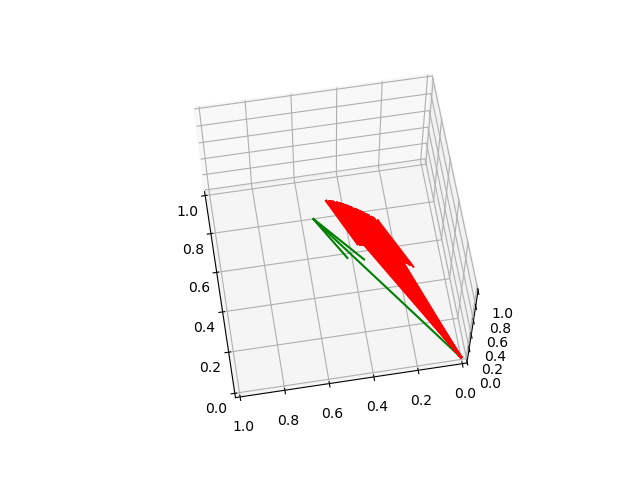
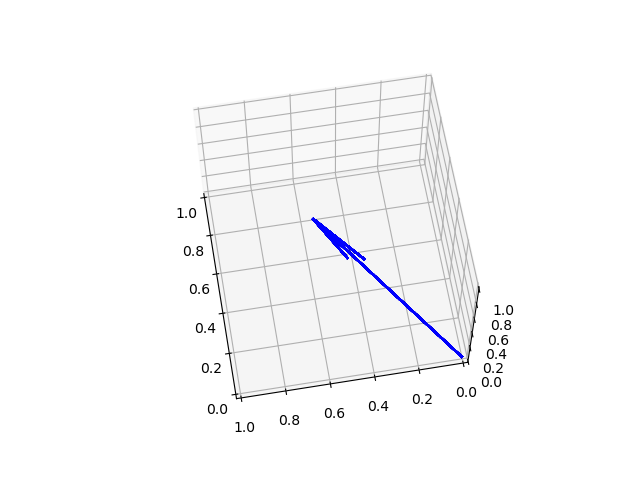
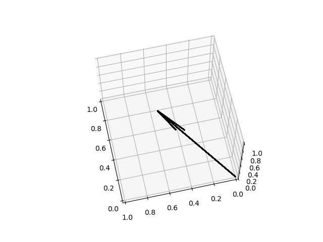
Figure 2: Direction of limit of conditioner in AdaGrad, RMSProp, and Adam (w/m) with different realizations of random initialization. In (a)-(c), the green vector stands for the isotropic direction (13,13,13)(\frac{1}{\sqrt{3}},\frac{1}{\sqrt{3}},\frac{1}{\sqrt{3}}). One red vector in (a) stands for direction of (𝒉∞A)−12(\boldsymbol{h}_{\infty}^{A})^{-\frac{1}{2}} in one experiment. Blue vector in (b) stands for direction of (𝒉∞R)−12(\boldsymbol{h}_{\infty}^{R})^{-\frac{1}{2}} under different initialization. Black vector in (c) stands for direction of (𝒉∞M)−12(\boldsymbol{h}_{\infty}^{M})^{-\frac{1}{2}} under different initialization. In (d), final values of the margin for the four algorithms are plotted (Adam (w/m) coincides with RMSProp).
Lemma 6.

For any t3>t2≥t1t_{3}>t_{2}\geq t_{1}, there exists a ξ∈[t2,t3]\xi\in[t_{2},t_{3}], such that

(⟨v^​(ξ),−∂sℒ~​(ξ)^⟩−2−1)≤𝒐⁡(1log⁡ρ~​(t3)−log⁡ρ~​(t2)),\displaystyle\left(\langle\hat{v}(\xi),-\widehat{{\partial}^{s}\tilde{\mathcal{L}}(\xi)}\rangle^{-2}-1\right)\leq\boldsymbol{o}\left(\frac{1}{\log\tilde{\rho}(t_{3})-\log\tilde{\rho}(t_{2})}\right),

and

‖𝒗^​(ξ)−𝒗^​(t2)‖≤𝒪⁡(log⁡ρ~​(t3)−log⁡ρ~​(t2)).\|\hat{\boldsymbol{v}}(\xi)-\hat{\boldsymbol{v}}(t_{2})\|\leq\mathcal{O}\left(\log\tilde{\rho}(t_{3})-\log\tilde{\rho}(t_{2})\right).

Therefore, given a sequence of parameter direction {𝒗^​(ti)}i=1∞\{\hat{\boldsymbol{v}}(t_{i})\}_{i=1}^{\infty} with limit 𝒗^\hat{\boldsymbol{v}}, we can always construct another sequence {ti′}i=1∞\{t_{i}^{\prime}\}_{i=1}^{\infty} with (1−⟨v^​(ti′),−∂sℒ~​(ti′)^⟩)\left(1-\langle\hat{v}(t_{i}^{\prime}),-\widehat{{\partial}^{s}\tilde{\mathcal{L}}(t_{i}^{\prime})}\rangle\right) and 𝒗^​(ti)−𝒗^​(ti′)\hat{\boldsymbol{v}}(t_{i})-\hat{\boldsymbol{v}}(t_{i}^{\prime}) converging to zero.

Combining Lemma 5 and 6, for any convergent direction 𝒗¯\bar{\boldsymbol{v}}, we can construct a series of {ti}i=1∞\{t_{i}\}_{i=1}^{\infty}, such that 𝒗^​(ti)\hat{\boldsymbol{v}}(t_{i}) is (εi,δi)(\varepsilon_{i},\delta_{i}) KKT point, with limi→∞𝒗^​(ti)=𝒗¯\lim_{i\rightarrow\infty}\hat{\boldsymbol{v}}(t_{i})=\bar{\boldsymbol{v}}, and limi→∞εi=limi→∞δi=0\lim_{i\rightarrow\infty}\varepsilon_{i}=\lim_{i\rightarrow\infty}\delta_{i}=0. On the other hand, constraints of (P)(P) satisfies Mangasarian-Fromovitz constraint qualification (see Appendix A.2), which ensures that 𝒗¯\bar{\boldsymbol{v}} is a KKT point of (P)(P), and completes the proof.

6 Experiments

6.1 Observations on Normalized Margin and Generalization Performance

In this section, we conduct experiments to verify the theoretical results. We train a homogeneous neural networks using AdaGrad, RMSProp and Adam (w/m) respectively. We adopt the homogeneous 4-layer convolutional neural network used in (Madry et al. 2018) as our model and use MNIST (LeCun 1998) as the dataset. We use default learning rate on PyTorch platform for all the algorithms and Adam (w/m) adopts the same learning rate as Adam. Because our theory is established for full batch gradient without randomness, we set minibatch size to be 10241024 which is relatively large to mimic the full batch gradient. We put more details on the network structure and the settings of hyper-parameters in Appendix F.1, where we also add standard SGD (with momentum) and Adam to observe influence of momentum.

We plot training accuracy, testing accuracy and training loss in Figure 1(a), 1(b), and 1(c). We also plot the value of the normalized margin during training in Figure 1(d). We have the following observations: (1) The normalized margins of AdaGrad, RMSProp and Adam (w/m) are lower bounded and the final normalized margin of AdaGrad is the lowest. It is consistent with our theoretical results. (2) The training loss of AdaGrad, RMSProp and Adam (w/m) goes to zero and AdaGrad achieves the lower test accuracy (the worse generalization), which shows the superiority of conditioners in RMSProp and Adam (w/m) on generalization. (3) Although our theory does not include momentum version of the algorithms, the normalized margin of SGD and Adam are also lower bounded , which shows potential on extension of our theory to momentum version.

6.2 Observations on Convergent Direction

In this section, we observe the direction of 𝒉∞\boldsymbol{h}_{\infty} on a simple case to illustrate that 𝒉∞\boldsymbol{h}_{\infty} of AdaGrad is anistropic and sensitive to initialization. The model we use is expressed as Φ⁡(𝒙,𝒘,v)=v​σ​(⟨𝒘,𝒙⟩)\Phi(\boldsymbol{x},\boldsymbol{w},v)=v\sigma(\langle\boldsymbol{w},\boldsymbol{x}\rangle), where x∈ℝ2,𝒘∈ℝ2x\in\mathbb{R}^{2},\boldsymbol{w}\in\mathbb{R}^{2} and v∈ℝv\in\mathbb{R} and σ⁡(x)\sigma(x) is the Leaky ReLU activation function, i.e., σ⁡(x)=x\sigma(x)=x for x≥0x\geq 0 and σ⁡(x)=x2\sigma(x)=\frac{x}{2} for x<0x<0.

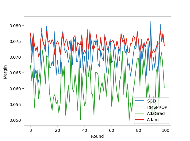
We repeat AdaGrad, RMSProp and Adam (w/m) for 100 rounds with different random seeds of initialization. We plot 𝒉∞−12\boldsymbol{h}^{-\frac{1}{2}}_{\infty} for AdaGrad, RMSProp and Adam in Figure 2 (a), (b) and (c), respectively. We can observe that the 𝒉∞−12\boldsymbol{h}^{-\frac{1}{2}}_{\infty} in AdaGrad are different for 100 runs and 𝒉∞−12\boldsymbol{h}^{-\frac{1}{2}}_{\infty} in RMSProp and Adam (w/m) are coincide. It indicates that 𝒉∞−12\boldsymbol{h}^{-\frac{1}{2}}_{\infty} in AdaGrad is sensitive to initialization. We also plot the value of the margin for the three algorithms under different initialization in Figure 2(d). We can observe that the margin of AdaGrad fluctuates under different initialization, while that for RMSProp and Adam (w/m) are smoother. We further show the relation between 𝒉∞−12\boldsymbol{h}^{-\frac{1}{2}}_{\infty} and the convergent direction of parameters in Appendix F.3. These results indicate that the convergent direction of AdaGrad is sensitive to initialization, which may hurt its generalization.

7 Conclusion

In this paper, we study the convergent direction of both continuous and discrete cases of adaptive optimization algorithms on homogeneous deep neural networks. We prove that RMSProp and Adam (w/m) will converge to the KKT points of the L2L^{2} max-margin problem, while AdaGrad does not. The main technical contribution of this paper is to propose a general framework for analyses of adaptive optimization algorithms’ convergent direction. In future, we will study how optimization techniques such as momentum, weight decay and stochastic noise in optimization algorithm influence the convergent direction.

References

  • Arora et al. (2019) Arora, S., Du, S. S., Hu, W., Li, Z., Salakhutdinov, R. R., and Wang, R. On exact computation with an infinitely wide neural net. In Advances in Neural Information Processing Systems, pp. 8141–8150, 2019.
  • Bartlett & Shawe-Taylor (1999) Bartlett, P. and Shawe-Taylor, J. Generalization performance of support vector machines and other pattern classifiers. Advances in Kernel methods—support vector learning, pp. 43–54, 1999.
  • Bartlett et al. (2017) Bartlett, P. L., Foster, D. J., and Telgarsky, M. Spectrally-normalized margin bounds for neural networks. In Proceedings of the 31st International Conference on Neural Information Processing Systems, pp. 6241–6250, 2017.
  • Brutzkus et al. (2018) Brutzkus, A., Globerson, A., Malach, E., and Shalev-Shwartz, S. Sgd learns over-parameterized networks that provably generalize on linearly separable data. In International Conference on Learning Representations, 2018.
  • Chen et al. (2018) Chen, J., Zhou, D., Tang, Y., Yang, Z., Cao, Y., and Gu, Q. Closing the generalization gap of adaptive gradient methods in training deep neural networks. arXiv preprint arXiv:1806.06763, 2018.
  • Choromanska et al. (2015) Choromanska, A., Henaff, M., Mathieu, M., Arous, G. B., and LeCun, Y. The loss surfaces of multilayer networks. In Artificial intelligence and statistics, pp. 192–204, 2015.
  • Clarke (1975) Clarke, F. H. Generalized gradients and applications. Transactions of the American Mathematical Society, 205:247–262, 1975.
  • Davis et al. (2020) Davis, D., Drusvyatskiy, D., Kakade, S., and Lee, J. D. Stochastic subgradient method converges on tame functions. Foundations of computational mathematics, 20(1):119–154, 2020.
  • Deng et al. (2013) Deng, L., Hinton, G., and Kingsbury, B. New types of deep neural network learning for speech recognition and related applications: An overview. In 2013 IEEE international conference on acoustics, speech and signal processing, pp. 8599–8603. IEEE, 2013.
  • Duchi et al. (2011) Duchi, J., Hazan, E., and Singer, Y. Adaptive subgradient methods for online learning and stochastic optimization. Journal of machine learning research, 12(7), 2011.
  • Gunasekar et al. (2018a) Gunasekar, S., Lee, J., Soudry, D., and Srebro, N. Characterizing implicit bias in terms of optimization geometry. In ICML, 2018a.
  • Gunasekar et al. (2018b) Gunasekar, S., Lee, J. D., Soudry, D., and Srebro, N. Implicit bias of gradient descent on linear convolutional networks. In Advances in Neural Information Processing Systems, pp. 9461–9471, 2018b.
  • Hinton et al. (2012) Hinton, G., Srivastava, N., and Swersky, K. Neural networks for machine learning lecture 6a overview of mini–batch gradient descent. 2012.
  • Ji & Telgarsky (2018) Ji, Z. and Telgarsky, M. Gradient descent aligns the layers of deep linear networks. In International Conference on Learning Representations, 2018.
  • Ji & Telgarsky (2019) Ji, Z. and Telgarsky, M. The implicit bias of gradient descent on nonseparable data. In Conference on Learning Theory, pp. 1772–1798, 2019.
  • Ji & Telgarsky (2020) Ji, Z. and Telgarsky, M. Directional convergence and alignment in deep learning. Advances in Neural Information Processing Systems, 33, 2020.
  • Jiang et al. (2019) Jiang, Y., Neyshabur, B., Mobahi, H., Krishnan, D., and Bengio, S. Fantastic generalization measures and where to find them. In International Conference on Learning Representations, 2019.
  • Keskar & Socher (2017) Keskar, N. S. and Socher, R. Improving generalization performance by switching from adam to sgd. arXiv preprint arXiv:1712.07628, 2017.
  • Kingma & Ba (2015) Kingma, D. P. and Ba, J. Adam: A method for stochastic optimization. In ICLR, 2015.
  • Kurdyka (1998) Kurdyka, K. On gradients of functions definable in o-minimal structures. In Annales de l’institut Fourier, volume 48, pp. 769–783, 1998.
  • LeCun (1998) LeCun, Y. The mnist database of handwritten digits. http://yann. lecun. com/exdb/mnist/, 1998.
  • Li et al. (2019) Li, Y., Fang, E. X., Xu, H., and Zhao, T. Implicit bias of gradient descent based adversarial training on separable data. In International Conference on Learning Representations, 2019.
  • Loshchilov & Hutter (2018) Loshchilov, I. and Hutter, F. Decoupled weight decay regularization. In International Conference on Learning Representations, 2018.
  • Luo et al. (2018) Luo, L., Xiong, Y., Liu, Y., and Sun, X. Adaptive gradient methods with dynamic bound of learning rate. In International Conference on Learning Representations, 2018.
  • Lyu & Li (2019) Lyu, K. and Li, J. Gradient descent maximizes the margin of homogeneous neural networks. In International Conference on Learning Representations, 2019.
  • Madry et al. (2018) Madry, A., Makelov, A., Schmidt, L., Tsipras, D., and Vladu, A. Towards deep learning models resistant to adversarial attacks. In International Conference on Learning Representations, 2018.
  • Nacson et al. (2019a) Nacson, M. S., Gunasekar, S., Lee, J., Srebro, N., and Soudry, D. Lexicographic and depth-sensitive margins in homogeneous and non-homogeneous deep models. In International Conference on Machine Learning, pp. 4683–4692. PMLR, 2019a.
  • Nacson et al. (2019b) Nacson, M. S., Lee, J., Gunasekar, S., Savarese, P. H. P., Srebro, N., and Soudry, D. Convergence of gradient descent on separable data. In The 22nd International Conference on Artificial Intelligence and Statistics, pp. 3420–3428. PMLR, 2019b.
  • Nacson et al. (2019c) Nacson, M. S., Srebro, N., and Soudry, D. Stochastic gradient descent on separable data: Exact convergence with a fixed learning rate. In The 22nd International Conference on Artificial Intelligence and Statistics, pp. 3051–3059. PMLR, 2019c.
  • Neyshabur et al. (2015) Neyshabur, B., Salakhutdinov, R. R., and Srebro, N. Path-sgd: Path-normalized optimization in deep neural networks. In Advances in Neural Information Processing Systems, pp. 2422–2430, 2015.
  • Neyshabur et al. (2018) Neyshabur, B., Bhojanapalli, S., and Srebro, N. A pac-bayesian approach to spectrally-normalized margin bounds for neural networks. In International Conference on Learning Representations, 2018.
  • Qian & Qian (2019) Qian, Q. and Qian, X. The implicit bias of adagrad on separable data. In Advances in Neural Information Processing Systems, pp. 7761–7769, 2019.
  • Reddi et al. (2018) Reddi, S., Zaheer, M., Sachan, D., Kale, S., and Kumar, S. Adaptive methods for nonconvex optimization. In Proceeding of 32nd Conference on Neural Information Processing Systems (NIPS 2018), 2018.
  • Ruder (2016) Ruder, S. An overview of gradient descent optimization algorithms. arXiv preprint arXiv:1609.04747, 2016.
  • Soudry et al. (2018) Soudry, D., Hoffer, E., Nacson, M. S., Gunasekar, S., and Srebro, N. The implicit bias of gradient descent on separable data. The Journal of Machine Learning Research, 19(1):2822–2878, 2018.
  • Stein & Shakarchi (2009) Stein, E. M. and Shakarchi, R. Real analysis: measure theory, integration, and Hilbert spaces. Princeton University Press, 2009.
  • Voulodimos et al. (2018) Voulodimos, A., Doulamis, N., Doulamis, A., and Protopapadakis, E. Deep learning for computer vision: A brief review. Computational intelligence and neuroscience, 2018, 2018.
  • Wilson et al. (2017) Wilson, A. C., Roelofs, R., Stern, M., Srebro, N., and Recht, B. The marginal value of adaptive gradient methods in machine learning. In Advances in neural information processing systems, pp. 4148–4158, 2017.
  • Witten & Frank (2005) Witten, I. H. and Frank, E. Data Mining: Practical Machine Learning Tools and Techniques, (Morgan Kaufmann Series in Data Management Systems). Morgan Kaufmann Publishers Inc., 2005.
  • Xu et al. (2018) Xu, T., Zhou, Y., Ji, K., and Liang, Y. When will gradient methods converge to max-margin classifier under relu models? arXiv preprint arXiv:1806.04339, 2018.
  • Young et al. (2018) Young, T., Hazarika, D., Poria, S., and Cambria, E. Recent trends in deep learning based natural language processing. ieee Computational intelligenCe magazine, 13(3):55–75, 2018.
  • Zhou et al. (2020) Zhou, P., Feng, J., Ma, C., Xiong, C., Hoi, S. C. H., et al. Towards theoretically understanding why sgd generalizes better than adam in deep learning. Advances in Neural Information Processing Systems, 33, 2020.
  • Zhuang et al. (2020) Zhuang, J., Tang, T., Ding, Y., Tatikonda, S. C., Dvornek, N., Papademetris, X., and Duncan, J. Adabelief optimizer: Adapting stepsizes by the belief in observed gradients. Advances in Neural Information Processing Systems, 33, 2020.

Appendix A Preliminaries

In this section, we provide some definitions and basic lemmas which will be used in the proof. The section is organized as follows: in Subsection A.1, we show general properties which exponential loss and logistic loss share; in Subsection A.2, (approximate) KKT conditions is defined and sufficient conditions of being an approximate KKT point is given; in Subsection A.3, we show how conditioners of AdaGrad, RMSProp, and Adam in continuous flow is formulated; in Subsection A.4, we introduce o-Minimal structure, definable set and definable functions, and show two Kurdyka-Lojasiewicz inequalities; in Subsection A.6, we show some basic definitions from Measure Theory, including measurable set and Lebesgue Integrability.

A.1 Property of Exponential and Logistic Loss

In this subsection, we provide several properties which both exponential and logistic loss possess. The properties of exponential and logistic loss can be described as the following proposition:

Proposition 1.

For ℓ∈{ℓe​x​p,ℓlog}\ell\in\{\ell_{exp},\ell_{\log}\}:

  • •

    There exists a C1C^{1} function ff, such that ℓ=e−f\ell=e^{-f};

  • •

    For any x∈ℝx\in\mathbb{R}, f′>0f^{\prime}>0. Therefore, ff is reversible, and f−1∈C1f^{-1}\in C^{1};

  • •

    f′​(x)​xf^{\prime}(x)x is non-decreasing for x∈(0,∞)x\in(0,\infty), and limx→∞f′​(x)​x=∞\lim_{x\rightarrow\infty}f^{\prime}(x)x=\infty;

  • •

    There exists a large enough xfx_{f} and a constant K≥1K\geq 1 ,such that,

    • –

      ∀θ∈[12,1),\forall\theta\in[\frac{1}{2},1), ∀x∈(xf,∞)\forall x\in(x_{f},\infty), and ∀y∈f−1​(xf,∞)\forall y\in f^{-1}(x_{f},\infty): (f−1)′​(x)≤K​(f−1)′​(θ​x)(f^{-1})^{\prime}(x)\leq K(f^{-1})^{\prime}(\theta x) and f′​(y)≤K​f′​(θ​y)f^{\prime}(y)\leq Kf^{\prime}(\theta y);

    • –

      For all y∈[xf,∞)y\in[x_{f},\infty), f⁡(x)f′​(x)∈[12​K​x,2​K​x]\frac{f(x)}{f^{\prime}(x)}\in[\frac{1}{2K}x,2Kx];

    • –

      For all x∈[f−1​(xf),∞)x\in[f^{-1}(x_{f}),\infty), f−1​(x)(f−1)′​(x)∈[12​K​x,2​K​x]\frac{f^{-1}(x)}{(f^{-1})^{\prime}(x)}\in[\frac{1}{2K}x,2Kx].

    • –

      f⁡(x)=Θ⁡(x)f(x)=\Theta(x) as x→∞x\rightarrow\infty.

All properties are easy to verify in Proposition 1 and we omit it here. For brevity, we will use g​(x)=f−1​(x)g(x)=f^{-1}(x) in the following proofs.

A.2 KKT Condition

Being a KKT point is a first order necessary condition for being an optimal point. We first give the definition of approximate KKT point for general optimization problem (Q)(Q).

Definition 2.

Consider the following optimization problem (Q)(Q) for 𝐱∈ℝd\boldsymbol{x}\in\mathbb{R}^{d}:

min⁡f⁡(𝒙)\displaystyle\min f(\boldsymbol{x})
subject to ​gi​(x)≤0,∀i∈[N],\displaystyle\text{subject to }g_{i}(x)\leq 0,\forall i\in[N],

where f,gif,g_{i} (i=1,⋯,Ni=1,\cdots,N): ℝd→ℝ\mathbb{R}^{d}\rightarrow\mathbb{R} are locally Lipschitz functions. We say that x∈ℝdx\in\mathbb{R}^{d} is a feasible point of (P)(P) if xx satisfies gi​(x)≤0g_{i}(x)\leq 0 for all i∈[N]i\in[N].

For any ε,δ>0\varepsilon,\delta>0, a feasible point of (Q)(Q) is an (ε,δ)(\varepsilon,\delta)-KKT point if there exists λi≥0\lambda_{i}\geq 0, 𝐤∈∂f⁡(𝐱)\mathbf{k}\in{\partial}f(\boldsymbol{x}), and 𝐡i∈∂gi​(𝐱)\boldsymbol{h}_{i}\in{\partial}g_{i}(\boldsymbol{x}) for all i∈[N]i\in[N] (we will slightly abuse ∂f⁡(𝐱){\partial}f(\boldsymbol{x}) to respresent a element in ∂f⁡(𝐱){\partial}f(\boldsymbol{x})) such that

1. ‖𝐤+∑i∈[N]λi​𝐡i​(𝐱)‖2≤ε\left\|\boldsymbol{k}+\sum_{i\in[N]}\lambda_{i}\boldsymbol{h}_{i}(\boldsymbol{x})\right\|_{2}\leq\varepsilon;

2. ∀i∈[N]:λi​gi​(𝐱)≥−δ\forall i\in[N]:\lambda_{i}g_{i}(\boldsymbol{x})\geq-\delta.

Specifically, when ε=δ=0\varepsilon=\delta=0, we call 𝐱\boldsymbol{x} a KKT point of (Q)(Q).

The following Mangasarian-Fromovitz constraint qualification (MFCQ) bridges (ε,δ)(\varepsilon,\delta) KKT points with KKT points.

Definition 3.

A feasible point 𝐱\boldsymbol{x} of (Q)(Q) is said to satisfy MFCQ if there exists 𝐚∈ℝd\boldsymbol{a}\in\mathbb{R}^{d} such that for every i∈[N]i\in[N] with gi​(𝐱)=0g_{i}(\boldsymbol{x})=0,

∀𝒉∈∂gi​(𝒙):⟨𝒉,𝒂⟩>0.\forall\boldsymbol{h}\in{\partial}g_{i}(\boldsymbol{x}):\langle\boldsymbol{h},\boldsymbol{a}\rangle>0.

MFCQ guarantees that the limit of approximate KKT point with convergent ε\varepsilon and δ\delta is a KKT point.

Lemma 7.

Suppose for any k∈ℕk\in\mathbb{N}, 𝐱k\boldsymbol{x}_{k} is a (εk,δk)(\varepsilon_{k},\delta_{k})-KKT point of (Q)(Q) defined in Definition 2. If limk→∞εk=0\lim_{k\rightarrow\infty}\varepsilon_{k}=0, limk→∞δk=0\lim_{k\rightarrow\infty}\delta_{k}=0, and limk→∞𝐱k=𝐱\lim_{k\rightarrow\infty}\boldsymbol{x}_{k}=\boldsymbol{x}, where the limit point 𝐱\boldsymbol{x} satisfies MFCQ, then 𝐱\boldsymbol{x} is a KKT point of (Q)(Q).

A.3 How is the Continuous Form of Conditioner Formulated?

In this subsection, we show how conditioners of the continuous case for AdaGrad, RMSProp, Adam (w/m) are derived. Both discrete updates of these optimizers can be written as

𝒘(t+1)−𝒘(t)∈−η1ε+ψ⁡(𝒎⁡(t),t)⊙∂sℒ(𝒘(t)),\displaystyle\boldsymbol{w}(t+1)-\boldsymbol{w}(t)\in-\eta\frac{1}{\sqrt{\varepsilon+\psi(\boldsymbol{m}(t),t)}}\odot\partial^{s}\mathcal{L}(\boldsymbol{w}(t)), (6)
𝒎⁡(t+1)−𝒎⁡(t)=ϕ⁡(𝒎⁡(t),∂sℒ⁡(𝒘⁡(t))),\displaystyle\boldsymbol{m}(t+1)-\boldsymbol{m}(t)=\phi(\boldsymbol{m}(t),\partial^{s}\mathcal{L}(\boldsymbol{w}(t))), (7)
𝒎⁡(0)=𝟎.\displaystyle\boldsymbol{m}(0)=\boldsymbol{0}.

where ∂sℒ⁡(𝒘⁡(t))∈∂ℒ⁡(𝒘⁡(t))\partial^{s}\mathcal{L}(\boldsymbol{w}(t))\in\partial\mathcal{L}(\boldsymbol{w}(t)). For AdaGrad, ϕ⁡(𝒎⁡(t),∂sℒ⁡(𝒘⁡(t)))=∂sℒ​(𝒘⁡(t))2\phi(\boldsymbol{m}(t),\partial^{s}\mathcal{L}(\boldsymbol{w}(t)))=\partial^{s}\mathcal{L}(\boldsymbol{w}(t))^{2}, ψ⁡(𝒎⁡(t),t)=𝒎⁡(t)\psi(\boldsymbol{m}(t),t)=\boldsymbol{m}(t); for RMSProp, ϕ⁡(𝒎⁡(t),∂sℒ⁡(𝒘⁡(t)))=(1−b)​(∂sℒ​(𝒘⁡(t))2−𝒎⁡(t))\phi(\boldsymbol{m}(t),\partial^{s}\mathcal{L}(\boldsymbol{w}(t)))=(1-b)(\partial^{s}\mathcal{L}(\boldsymbol{w}(t))^{2}-\boldsymbol{m}(t)), ψ⁡(𝒎⁡(t),t)=𝒎⁡(t)\psi(\boldsymbol{m}(t),t)=\boldsymbol{m}(t); for Adam (w/m), ϕ⁡(𝒎⁡(t),∂sℒ⁡(𝒘⁡(t)))=(1−b)​(∂sℒ​(𝒘⁡(t))2−𝒎⁡(t))\phi(\boldsymbol{m}(t),\partial^{s}\mathcal{L}(\boldsymbol{w}(t)))=(1-b)(\partial^{s}\mathcal{L}(\boldsymbol{w}(t))^{2}-\boldsymbol{m}(t)), ψ⁡(𝒎⁡(t),t)=𝒎⁡(t)1−bt\psi(\boldsymbol{m}(t),t)=\frac{\boldsymbol{m}(t)}{1-b^{t}}.

One can easily observe that eqs. (6) and (7) is a discretization of the following equations:

d​𝒘​(t)d​t=−1ε+ψ⁡(𝒎⁡(t),t)⊙∂sℒ(𝒘(t)),\displaystyle\frac{\mathrm{d}\boldsymbol{w}(t)}{\mathrm{d}t}=-\frac{1}{\sqrt{\varepsilon+\psi(\boldsymbol{m}(t),t)}}\odot\partial^{s}\mathcal{L}(\boldsymbol{w}(t)), (8)
d​𝒎​(t)d​t=ϕ⁡(𝒎⁡(t),∂sℒ⁡(𝒘⁡(t))),\displaystyle\frac{\mathrm{d}\boldsymbol{m}(t)}{\mathrm{d}t}=\phi(\boldsymbol{m}(t),\partial^{s}\mathcal{L}(\boldsymbol{w}(t))), (9)
𝒎⁡(0)=𝟎.\displaystyle\boldsymbol{m}(0)=\boldsymbol{0}.

As for AdaGrad,

d​𝒎​(t)d​t=∂sℒ​(𝒘⁡(t))2,\frac{\mathrm{d}\boldsymbol{m}(t)}{\mathrm{d}t}=\partial^{s}\mathcal{L}(\boldsymbol{w}(t))^{2},

which leads to

𝒎⁡(t)=∫0t∂sℒ​(𝒘⁡(τ))2​𝑑τ,\boldsymbol{m}(t)=\int_{0}^{t}\partial^{s}\mathcal{L}(\boldsymbol{w}(\tau))^{2}\mathrm{d}\tau,

and

d​𝒘​(t)d​t=−1ε+∫0t∂sℒ​(𝒘⁡(τ))2​𝑑τ⊙∂sℒ(𝒘(t))\frac{\mathrm{d}\boldsymbol{w}(t)}{\mathrm{d}t}=-\frac{1}{\sqrt{\varepsilon+\int_{0}^{t}\partial^{s}\mathcal{L}(\boldsymbol{w}(\tau))^{2}\mathrm{d}\tau}}\odot\partial^{s}\mathcal{L}(\boldsymbol{w}(t))

As for RMSProp and Adam

d​𝒎​(t)d​t=(1−b)​(∂sℒ​(𝒘⁡(t))2−𝒎⁡(t)).\frac{\mathrm{d}\boldsymbol{m}(t)}{\mathrm{d}t}=(1-b)(\partial^{s}\mathcal{L}(\boldsymbol{w}(t))^{2}-\boldsymbol{m}(t)).

By solving the above differential equation, we have

d​e(1−b)​t​𝒎​(t)d​t=e(1−b)​t​(1−b)​∂sℒ​(𝒘⁡(t))2,\frac{\mathrm{d}e^{(1-b)t}\boldsymbol{m}(t)}{\mathrm{d}t}=e^{(1-b)t}(1-b)\partial^{s}\mathcal{L}(\boldsymbol{w}(t))^{2},

which by integration implies

𝒎⁡(t)=∫0te−(1−b)​(t−τ)​(1−b)​∂sℒ​(𝒘⁡(τ))2​𝑑τ.\boldsymbol{m}(t)=\int_{0}^{t}e^{-(1-b)(t-\tau)}(1-b)\partial^{s}\mathcal{L}(\boldsymbol{w}(\tau))^{2}\mathrm{d}\tau.

Therefore, for RMSProp, the continuous flow is

d​𝒘​(t)d​t=−1ε+∫0te−(1−b)​(t−τ)​(1−b)​∂sℒ​(𝒘⁡(τ))2​𝑑τ⊙∂sℒ(𝒘(t));\frac{\mathrm{d}\boldsymbol{w}(t)}{\mathrm{d}t}=-\frac{1}{\sqrt{\varepsilon+\int_{0}^{t}e^{-(1-b)(t-\tau)}(1-b)\partial^{s}\mathcal{L}(\boldsymbol{w}(\tau))^{2}\mathrm{d}\tau}}\odot\partial^{s}\mathcal{L}(\boldsymbol{w}(t));

while for Adam (w/m), the continuous flow is

d​𝒘​(t)d​t=−1ε+∫0te−(1−b)​(t−τ)​(1−b)​∂sℒ​(𝒘⁡(τ))2​𝑑τ1−bt⊙∂sℒ(𝒘(t)).\frac{\mathrm{d}\boldsymbol{w}(t)}{\mathrm{d}t}=-\frac{1}{\sqrt{\varepsilon+\frac{\int_{0}^{t}e^{-(1-b)(t-\tau)}(1-b)\partial^{s}\mathcal{L}(\boldsymbol{w}(\tau))^{2}\mathrm{d}\tau}{1-b^{t}}}}\odot\partial^{s}\mathcal{L}(\boldsymbol{w}(t)).

A.4 o-Minimal Structure and Definable functions

Here we define o-Minimal structure and definable functions which we omit in Theorem 3.

Definition 4 (Appendix B, Ji & Telgarsky 2020).

An o-minimal structure is a collection 𝒮={𝒮n}n=1∞\mathcal{S}=\{\mathcal{S}_{n}\}_{n=1}^{\infty}, where each 𝒮n\mathcal{S}_{n} is a set of subsets of ℝn\mathbb{R}_{n} satisfying the following conditions: 1. 𝒮1\mathcal{S}_{1} is the collection of all finite unions of open intervals and points;
2. 𝒮n\mathcal{S}_{n} includes the zero sets of all polynomials on ℝn\mathbb{R}_{n};
3. 𝒮n\mathcal{S}_{n} is closed under finite union, finite intersection, and complement;
4. 𝒮\mathcal{S} is closed under Cartesian products: if A∈𝒮mA\in\mathcal{S}_{m} and B∈𝒮nB\in\mathcal{S}_{n}, then A×B∈𝒮m+nA\times B\in\mathcal{S}_{m+n};
5. 𝒮\mathcal{S} is closed under projection Πn\Pi_{n} onto the first nn coordinates: if A∈𝒮n+1A\in\mathcal{S}_{n+1}, then Πn​(A)∈𝒮n\Pi_{n}(A)\in\mathcal{S}_{n}.

A definable function on above o-Minimal Structure can be defined as follows:

Definition 5 (Appendix B, Ji & Telgarsky 2020).

A function f:D→ℝmf:D\rightarrow\mathbb{R}^{m} with D⊂ℝnD\subset\mathbb{R}^{n} is definable if the graph of ff is in 𝒮n+m\mathcal{S}_{n+m}.

A natural question is: which function is definable? The next Lemma helps to solve this question.

Lemma 8 (Lemma B.2, Ji & Telgarsky 2020).
  • •

    All polynomials are definable, therefore, linear or other polynomial activation is definable;

  • •

    If both f⁡(x)f(x) and g⁡(x)g(x) are definable, min⁡f⁡(x),g⁡(x)\min{f(x),g(x)} and max⁡f⁡(x),g⁡(x)\max{f(x),g(x)} are definable, therefore, ReLU activation is definable;

  • •

    If fi​(x):D→ℝf_{i}(x):D\rightarrow\mathbb{R} (i=1,2,⋯,ni=1,2,\cdots,n) is definable, then 𝒇⁡(x)=(f1​(x),f2​(x),⋯,fn​(x))\boldsymbol{f}(x)=(f_{1}(x),f_{2}(x),\cdots,f_{n}(x)) is definable.

  • •

    Suppose there exists k,d0,d1,⋯,dL>0k,d_{0},d_{1},\cdots,d_{L}>0, and LL definable functions (g1,g2,⋯,gL)(g_{1},g_{2},\cdots,g_{L}), where gj:→ℝd0×⋯×ℝdj−1×ℝk→ℝdjg_{j}:\rightarrow\mathbb{R}^{d_{0}}\times\cdots\times\mathbb{R}^{d_{j-1}}\times\mathbb{R}^{k}\rightarrow\mathbb{R}^{d_{j}}. Let h1​(x,W)​=△​g1​(x,W)h_{1}(x,W)\overset{\triangle}{=}g_{1}(x,W), and for 2≤j≤L2\leq j\leq L,

    hj​(x,W):=gj​(x,h1​(x,W),…,hj−1​(x,W),W),h_{j}(x,W):=g_{j}\left(x,h_{1}(x,W),\ldots,h_{j-1}(x,W),W\right),

    then all hjh_{j} are definable. Therefore, neural networks with polynomial and ReLU activation, convolutional and max-pooling layers, and skip connections are definable.

An important property for definable function is Kurdyka-Lojasiewicz inequality, which can bound gradient of definable function in a small region. Here we present two Kurdyka-Lojasiewicz inequalities given by (Ji & Telgarsky 2020):

Lemma 9 (Lemma 3.6, Ji & Telgarsky 2020).

Given a locally Lipschitz definable function ff with an open domain D∈{x|‖x‖>1}D\in\{x|\|x\|>1\}, for any cc, η>0\eta>0, there exists a>0a>0 and a definable desingularizing function Ψ\Psi on [0,a)[0,a) (that is, Ψ⁡(x)∈C1​((0,a))∩C0​([0,a))\Psi(x)\in C^{1}((0,a))\cap C^{0}([0,a)) with Ψ⁡(0)=0\Psi(0)=0), such that,

Ψ′​(f⁡(x))​‖x‖​‖∂¯​f​(x)‖≥1, if ​f​(x)∈(0,a), and ​‖∂¯⟂​f​(x)‖≥c​‖x‖η​‖∂¯\⁣\​f​(x)‖,\Psi^{\prime}(f(x))\|x\|\|\bar{\partial}f(x)\|\geq 1,\text{ if }f(x)\in(0,a),\text{ and }\left\|\bar{\partial}_{\perp}f(x)\right\|\geq c\|x\|^{\eta}\left\|\bar{\partial}_{\backslash\backslash}f(x)\right\|,

where ∂¯​f​(x)\bar{\partial}f(x) is the unique one with the smallest norm in ∂f⁡(x)\partial f(x), ∂¯\⁣\​f​(x)\bar{\partial}_{\backslash\backslash}f(x) is the projection of ∂¯​f​(x)\bar{\partial}f(x) to xx and ∂¯⟂​f​(x)=∂¯​f​(x)−∂¯\⁣\​f​(x)\bar{\partial}_{\perp}f(x)=\bar{\partial}f(x)-\bar{\partial}_{\backslash\backslash}f(x) is the remaining term

Lemma 10 (Lemma 3.7, Ji & Telgarsky 2020).

Given a locally Lipschitz definable function ff with an open domain D⊂{x|‖x‖>1}D\subset\{x|\|x\|>1\}, for any λ>0\lambda>0, there exists a>0a>0, and a definable desingularizing function Ψ\Psi on [0,a)[0,a) such that

max⁡{1,2λ}​Ψ′​(f⁡(x))​‖x‖1+λ​‖∂¯​f​(x)‖≥1, if ​f​(x)∈(0,a).\max\left\{1,\frac{2}{\lambda}\right\}\Psi^{\prime}(f(x))\|x\|^{1+\lambda}\|\bar{\partial}f(x)\|\geq 1,\text{ if }f(x)\in(0,a).

At the end of this subsection, we show that definability actually guarantees that Φ\Phi admits a chain rule, which is formally stated as following:

Lemma 11 (Lemma B.9, Ji & Telgarsky 2020).

Given a locally Lipschitz definable f:D→ℝf:D\rightarrow\mathbb{R} with an open domain DD, for any interval II and any arc z:I→Dz:I\rightarrow D, it holds for a.e. t∈It\in I that

d​f​(zt)d​t=⟨zt∗,d​ztd​t⟩, for all ​zt∗∈∂f⁡(zt).\frac{\mathrm{d}f\left(z_{t}\right)}{\mathrm{d}t}=\left\langle z_{t}^{*},\frac{\mathrm{d}z_{t}}{\mathrm{d}t}\right\rangle,\quad\text{ for all }z_{t}^{*}\in\partial f\left(z_{t}\right).

Therefore, if we are deal with definable neural networks Φ\Phi as in Theorem 3, we no longer need to assume Φ\Phi admits a chain rule which is already guaranteed by lemma 11.

A.5 Discussion of the influence of initialization on the solution of PAP^{A}

For AdaGrad, 𝒉∞−2\boldsymbol{h}^{-2}_{\infty} is defined as ε𝟏p+∑t=0∞∇ℒ(𝒘(t))2\varepsilon\mathbf{1}_{p}+\sum_{t=0}^{\infty}\nabla\mathcal{L}(\boldsymbol{w}(t))^{2}, which is the sum of squared gradients along the trajectory. Intuitively, as the initialization changes, the trajectory changes respectively, and so does the direction of 𝒉∞\boldsymbol{h}_{\infty}. This intuition can be further verified by Experiment in Section 6.2, where we plot the direction of 𝒉∞−12\boldsymbol{h}^{-\frac{1}{2}}_{\infty} as the initialization changes.

Refer to caption
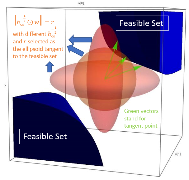
Figure 3: How 𝒉∞\boldsymbol{h}_{\infty} influence convergence direction of 𝒘\boldsymbol{w}

Furthermore, how 𝒉∞\boldsymbol{h}_{\infty} influence the max-margin problem can be interpreted as follows: optimizing ‖𝒉∞−12⊙𝒘‖2\|\boldsymbol{h}_{\infty}^{-\frac{1}{2}}\odot\boldsymbol{w}\|^{2} with constraints is equivalent to find the radius rr of ellipsoid ‖𝒉∞−12⊙𝒘‖2=r2\|\boldsymbol{h}_{\infty}^{-\frac{1}{2}}\odot\boldsymbol{w}\|^{2}=r^{2} when the ellipsoid is tangent to the feasible set. This intuition is visualized in Figure 3. One can easily observe that as the direction of 𝒉∞\boldsymbol{h}_{\infty} changes, the direction of the tangent point changes.

A.6 Basic knowledge from Measure Theory

In this section, we present basic definitions of measurable set, measurable functions and Lebesgue Integrability. These definition involves use of exterior measure and Borel set in Euclidean space, which we omit them here. Readers interested in measure theory can refer to (Stein & Shakarchi 2009) for details.

Definition 6 (Stein & Shakarchi 2009, Chapter 1, page 16).

A subset EE of ℝd\mathbb{R}^{d}is Lesbesgue measurable, or simply measurable, if for any ε>0\varepsilon>0, there exists an open set GG, with E⊂GE\subset G, and

m∗​(G/E)≤ε,m_{*}(G/E)\leq\varepsilon,

where m∗m_{*} is the exterior measure on ℝd\mathbb{R}^{d}.

Definition 7 (Stein & Shakarchi 2009, Chapter 1, page 28).

A function ff on a measurable subset EE of ℝd\mathbb{R}^{d} is measurable if for all a∈ℝa\in\mathbb{R}, the set

f−1([−∞,a))={x∈E:f(x)<a}f^{-1}([-\infty,a))=\{x\in E:f(x)<a\}

is measurable.

Definition 8 (Stein & Shakarchi 2009, Chapter 1, page 64).

A measurable function ff defined on a measurable subset of ℝd\mathbb{R}^{d} is Lesbesgue integrable if

∫E|f⁡(x)|​𝑑m​(x)<∞.\int_{E}|f(x)|\mathrm{d}m(x)<\infty.

Appendix B Proof of Results for Adaptive Algorithms in Continuous Case

This section collects proof of Theorem 2, Theorem 4, Theorem 5, and also contains proof of Theorem 6 and Theorem 7. Organization of this section is as follows: In Subsection B.1, we present proof of Theorems 4 and Theorem 5; in Subsection B.2, we present proof of Theorem 2 based on the proof skeleton in Section 5; in Subsection B.3, we prove Theorem 6 and Theorem 7 based on 2, Theorem 4, Theorem 5; finally, in Subsection B.4, we provide tight convergence rate of loss and parameter norm in adaptive gradient flows.

B.1 Proof of Theorem 4 and Theorem 5: Transition from Continuous Adaptive Algorithms to Adaptive Gradient Flow

B.1.1 Proof of Theorem 4

The proof of Theorem 4 is divided into two stages: we first prove convergence of 𝒉A​(t)\boldsymbol{h}^{A}(t) and 𝜷A​(t)\boldsymbol{\beta}^{A}(t); then we show d​𝒗A​(t)d​t=−𝜷A(t)⊙∂sℒ~A(𝒗A(t))\frac{\mathrm{d}\boldsymbol{v}^{A}(t)}{\mathrm{d}t}=-\boldsymbol{\beta}^{A}(t)\odot\partial^{s}\tilde{\mathcal{L}}^{A}(\boldsymbol{v}^{A}(t)) satisfies adaptive gradient flow, and is equivalent to AdaGrad flow.

We first show ∫0∞∂sℒ​(𝒘⁡(t))2​𝑑τ\int_{0}^{\infty}\partial^{s}\mathcal{L}(\boldsymbol{w}(t))^{2}\mathrm{d}\tau is bounded.

Lemma 12.

For AdaGrad flow defined as eq. (4) with 𝐡=𝐡A\boldsymbol{h}=\boldsymbol{h}^{A},

∫0∞(∂sℒ(𝒘(τ)))i2dτ<∞,i=1,⋯,p.\int_{0}^{\infty}(\partial^{s}\mathcal{L}(\boldsymbol{w}(\tau)))_{i}^{2}\mathrm{d}\tau<\infty,i=1,\cdots,p.
Proof.

We use reduction of absurdity. If there exists an ii, such that, ∫0∞(∂sℒ⁡(𝒘⁡(τ)))i2​𝑑τ\int_{0}^{\infty}(\partial^{s}\mathcal{L}(\boldsymbol{w}(\tau)))_{i}^{2}\mathrm{d}\tau diverges, by equivalence of integral convergence, then

∫0∞(∂sℒ⁡(𝒘⁡(t)))i2ε+∫0t(∂sℒ⁡(𝒘⁡(τ)))i2​𝑑τ​𝑑t=∞.\int_{0}^{\infty}\frac{(\partial^{s}\mathcal{L}(\boldsymbol{w}(t)))_{i}^{2}}{\varepsilon+\int_{0}^{t}(\partial^{s}\mathcal{L}(\boldsymbol{w}(\tau)))_{i}^{2}\mathrm{d}\tau}\mathrm{d}t=\infty.

Since ∫0∞(∂sℒ⁡(𝒘⁡(τ)))i2​𝑑τ=∞\int_{0}^{\infty}(\partial^{s}\mathcal{L}(\boldsymbol{w}(\tau)))_{i}^{2}\mathrm{d}\tau=\infty, when tt is large enough,

ε+∫0t(∂sℒ⁡(𝒘⁡(τ)))i2​𝑑τ>ε+∫0t(∂sℒ⁡(𝒘⁡(τ)))i2​𝑑τ.\varepsilon+\int_{0}^{t}(\partial^{s}\mathcal{L}(\boldsymbol{w}(\tau)))_{i}^{2}\mathrm{d}\tau>\sqrt{\varepsilon+\int_{0}^{t}(\partial^{s}\mathcal{L}(\boldsymbol{w}(\tau)))_{i}^{2}\mathrm{d}\tau}.

Therefore,

∫0∞(∂sℒ⁡(𝒘⁡(t)))i2ε+∫0t(∂sℒ⁡(𝒘⁡(τ)))i2​𝑑τ​𝑑t=∞.\int_{0}^{\infty}\frac{(\partial^{s}\mathcal{L}(\boldsymbol{w}(t)))_{i}^{2}}{\sqrt{\varepsilon+\int_{0}^{t}(\partial^{s}\mathcal{L}(\boldsymbol{w}(\tau)))_{i}^{2}\mathrm{d}\tau}}\mathrm{d}t=\infty.

By integrating d​ℒ​(𝒘⁡(t))d​t\frac{\mathrm{d}\mathcal{L}(\boldsymbol{w}(t))}{\mathrm{d}t},

ℒ⁡(𝒘⁡(0))−ℒ⁡(𝒘⁡(t))\displaystyle\mathcal{L}(\boldsymbol{w}(0))-\mathcal{L}(\boldsymbol{w}(t)) =−∫0td​ℒ​(𝒘⁡(τ))d​τdτ\displaystyle=-\int_{0}^{t}\frac{\mathrm{d}\mathcal{L}(\boldsymbol{w}(\tau))}{\mathrm{d}\tau}\mathrm{d}\tau
=−∫0t⟨∂sℒ(𝒘(τ)),d​𝒘​(τ)d​τ⟩dτ\displaystyle=-\int_{0}^{t}\left\langle\partial^{s}\mathcal{L}(\boldsymbol{w}(\tau)),\frac{\mathrm{d}\boldsymbol{w}(\tau)}{\mathrm{d}\tau}\right\rangle\mathrm{d}\tau
=∫0t⟨∂sℒ⁡(𝒘⁡(τ)),𝒉A​(τ)⊙∂sℒ⁡(𝒘⁡(τ))⟩​𝑑τ\displaystyle=\int_{0}^{t}\langle\partial^{s}\mathcal{L}(\boldsymbol{w}(\tau)),\boldsymbol{h}^{A}(\tau)\odot\partial^{s}\mathcal{L}(\boldsymbol{w}(\tau))\rangle\mathrm{d}\tau
=∑i=1p∫0t(∂sℒ⁡(𝒘⁡(s)))i2ε+∫0t(∂sℒ⁡(𝒘⁡(τ)))i2​𝑑τ​𝑑s\displaystyle=\sum_{i=1}^{p}\int_{0}^{t}\frac{(\partial^{s}\mathcal{L}(\boldsymbol{w}(s)))_{i}^{2}}{\sqrt{\varepsilon+\int_{0}^{t}(\partial^{s}\mathcal{L}(\boldsymbol{w}(\tau)))_{i}^{2}\mathrm{d}\tau}}\mathrm{d}s
=∞,\displaystyle=\infty,

which leads to a contradictory, since ℒ⁡(𝝎⁡(0))−ℒ⁡(𝝎⁡(t))\mathcal{L}(\boldsymbol{\omega}(0))-\mathcal{L}(\boldsymbol{\omega}(t)) is upper bounded by ℒ⁡(𝝎⁡(0))\mathcal{L}(\boldsymbol{\omega}(0)).

The proof is completed. ∎

Now we are ready to prove Theorem 4.

Theorem 9 (Theorem 4, restated).

Define 𝐡∞=limt→∞𝐡A​(t)\boldsymbol{h}_{\infty}=\lim_{t\rightarrow\infty}\boldsymbol{h}^{A}(t). Then 𝐡∞\boldsymbol{h}_{\infty} has no zero elements. Let

𝒗A(t)=𝒉∞−1/2⊙𝒘(t),\displaystyle\boldsymbol{v}^{A}(t)=\boldsymbol{h}_{\infty}^{-1/2}\odot\boldsymbol{w}(t),
𝜷A​(t)=𝒉∞−1⊙𝒉A​(t),\displaystyle\boldsymbol{\beta}^{A}(t)=\boldsymbol{h}_{\infty}^{-1}\odot\boldsymbol{h}^{A}(t),
ℒ~A​(𝒗)=ℒ⁡(𝒉∞12⊙𝒗).\displaystyle\tilde{\mathcal{L}}^{A}(\boldsymbol{v})=\mathcal{L}(\boldsymbol{h}_{\infty}^{\frac{1}{2}}\odot\boldsymbol{v}).

We have

d​𝒗A​(t)d​t=−𝜷A(t)⊙∂sℒ~A(𝒗A(t)),\frac{\mathrm{d}\boldsymbol{v}^{A}(t)}{\mathrm{d}t}=-\boldsymbol{\beta}^{A}(t)\odot\partial^{s}\tilde{\mathcal{L}}^{A}(\boldsymbol{v}^{A}(t)), (10)

while limt→∞𝛃A​(t)=1\lim_{t\rightarrow\infty}\boldsymbol{\beta}^{A}(t)=1, and d​log⁡𝛃A​(t)d​t\frac{\mathrm{d}\log\boldsymbol{\beta}^{A}(t)}{\mathrm{d}t} is Lebesgue integrable.

Proof.

Since

𝒉∞=1ε​𝟏p+∫0∞(∂sℒ⁡(𝒘⁡(τ)))i2​𝑑τ,\boldsymbol{h}_{\infty}=\frac{1}{\sqrt{\varepsilon\mathbf{1}_{p}+\int_{0}^{\infty}(\partial^{s}\mathcal{L}(\boldsymbol{w}(\tau)))_{i}^{2}\mathrm{d}\tau}},

by Lemma 12, 𝒉∞\boldsymbol{h}_{\infty} has no zero elements.

We then prove eq. (10) by direct calculation.

d​𝒗A​(t)d​t\displaystyle\frac{\mathrm{d}\boldsymbol{v}^{A}(t)}{\mathrm{d}t} =𝒉∞−1/2⊙d​𝒘​(t)d​t\displaystyle=\boldsymbol{h}_{\infty}^{-1/2}\odot\frac{d\boldsymbol{w}(t)}{\mathrm{d}t}
=−𝒉∞−1/2⊙𝒉A(t)⊙∂sℒ(𝒘(t))\displaystyle=-\boldsymbol{h}_{\infty}^{-1/2}\odot\boldsymbol{h}^{A}(t)\odot\partial^{s}\mathcal{L}(\boldsymbol{w}(t))
=−𝒉∞−1/2⊙𝒉A(t)⊙𝒉∞−1/2⊙𝒉∞1/2⊙∂𝒘sℒ~A(𝒉∞−1/2⊙𝒘(t))\displaystyle=-\boldsymbol{h}_{\infty}^{-1/2}\odot\boldsymbol{h}^{A}(t)\odot\boldsymbol{h}_{\infty}^{-1/2}\odot\boldsymbol{h}_{\infty}^{1/2}\odot\partial^{s}_{\boldsymbol{w}}\tilde{\mathcal{L}}^{A}(\boldsymbol{h}_{\infty}^{-1/2}\odot\boldsymbol{w}(t))
=−𝜷A(t)⊙∂𝒉∞−1/2⊙𝒘(t)sℒ~A(𝒉∞−1/2⊙𝒘(t))\displaystyle=-\boldsymbol{\beta}^{A}(t)\odot\partial^{s}_{\boldsymbol{h}_{\infty}^{-1/2}\odot\boldsymbol{w}(t)}\tilde{\mathcal{L}}^{A}(\boldsymbol{h}_{\infty}^{-1/2}\odot\boldsymbol{w}(t))
=−𝜷A(t)⊙∂𝒗⁡(t)sℒ~A(𝒗(t)),\displaystyle=-\boldsymbol{\beta}^{A}(t)\odot\partial^{s}_{\boldsymbol{v}(t)}\tilde{\mathcal{L}}^{A}(\boldsymbol{v}(t)),

which completes the proof of eq. ( 10).

limt→∞𝜷A​(t)=1\lim_{t\rightarrow\infty}\boldsymbol{\beta}^{A}(t)=1 can be derived directly by convergence of 𝒉A​(t)\boldsymbol{h}^{A}(t), while since

d​log⁡𝜷A​(t)d​t=d​log⁡𝒉A​(t)d​t​≤(∗)​𝟎,\frac{\mathrm{d}\log\boldsymbol{\beta}^{A}(t)}{\mathrm{d}t}=\frac{\mathrm{d}\log\boldsymbol{h}^{A}(t)}{\mathrm{d}t}\overset{(*)}{\leq}\mathbf{0},

where inequality (∗)(*) is due to 𝒉A\boldsymbol{h}^{A} is non-increasing.

Therefore,

∫0∞|d​log⁡𝜷A​(t)d​t|dt=−∫0∞d​log⁡𝜷A​(t)d​tdt=log𝜷A(0)<∞.\int_{0}^{\infty}\left|\frac{\mathrm{d}\log\boldsymbol{\beta}^{A}(t)}{\mathrm{d}t}\right|\mathrm{d}t=-\int_{0}^{\infty}\frac{\mathrm{d}\log\boldsymbol{\beta}^{A}(t)}{\mathrm{d}t}\mathrm{d}t=\log\boldsymbol{\beta}^{A}(0)<\infty.

The proof is completed. ∎

B.1.2 Proof of Theorem 5

We first prove Theorem 5 for RMSProp, and then extend the proof for Adam (w/m) and other Adam-like optimizers. The proof strategy is similar with AdaGrad: we first prove convergence of 𝒉R​(t)\boldsymbol{h}^{R}(t) and integrability d​log⁡𝜷R​(t)d​t\frac{\mathrm{d}\log\boldsymbol{\beta}^{R}(t)}{\mathrm{d}t}; then we show d​𝒗R​(t)d​t=−𝜷R(t)⊙∂sℒ~R(𝒗R(t))\frac{\mathrm{d}\boldsymbol{v}^{R}(t)}{\mathrm{d}t}=-\boldsymbol{\beta}^{R}(t)\odot\partial^{s}\tilde{\mathcal{L}}^{R}(\boldsymbol{v}^{R}(t)) is equivalent to RMSProp flow, and satisfies adaptive gradient flow.

However, for RMSProp flow, the convergence of 𝒉R\boldsymbol{h}^{R} requires more effort. We start from the following lemma, which bounds Fi​(t)​=△​∫0t(1−b)​bt−τ​(∂sℒ⁡(𝒘⁡(τ)))i2​𝑑τF_{i}(t)\overset{\triangle}{=}\int_{0}^{t}(1-b)b^{t-\tau}(\partial^{s}\mathcal{L}(\boldsymbol{w}(\tau)))_{i}^{2}\mathrm{d}\tau (i∈[p]i\in[p]).

Lemma 13.

For RMSProp flow defined as eq. (4) with 𝐡=𝐡R\boldsymbol{h}=\boldsymbol{h}^{R} , Fi​(t)F_{i}(t) is bounded (i=1,2,⋯,pi=1,2,\cdots,p), that is,

lim¯t→∞​Fi​(t)<∞.\overline{\lim}_{t\rightarrow\infty}F_{i}(t)<\infty.
Proof.

When b=1b=1, Fi​(t)=0F_{i}(t)=0 for all tt and ii, which trivially yields the claim. When b≠1b\neq 1, we use reduction of absurdity. If there exists an ii, such that, lim¯t→∞​Fi​(t)=∞\overline{\lim}_{t\rightarrow\infty}F_{i}(t)=\infty, then tk​=△​inf{t:Fi​(t)≥k}<∞t_{k}\overset{\triangle}{=}\inf\{t:F_{i}(t)\geq k\}<\infty holds. Furthermore, since ℒ\mathcal{L} is locally Lipschitz with respect to 𝒘\boldsymbol{w}, gi​(t)g_{i}(t) is locally bounded for any tt, which leads to the absolute continuity of FiF_{i}. Therefore, since Fi​(0)=0F_{i}(0)=0, tkt_{k} monotonously increases.

Therefore, we have that

∫tktk+1(∂sℒ⁡(𝒘⁡(t)))i2ε+Fi​(t)​𝑑t\displaystyle\int_{t_{k}}^{t_{k+1}}\frac{(\partial^{s}\mathcal{L}(\boldsymbol{w}(t)))_{i}^{2}}{\sqrt{\varepsilon+F_{i}(t)}}\mathrm{d}t ≥∫tktk+1(∂sℒ⁡(𝒘⁡(t)))i2ε+k+1​𝑑t\displaystyle\geq\int_{t_{k}}^{t_{k+1}}\frac{(\partial^{s}\mathcal{L}(\boldsymbol{w}(t)))_{i}^{2}}{\sqrt{\varepsilon+k+1}}\mathrm{d}t
=1ε+k+1​∫tktk+1(∂sℒ⁡(𝒘⁡(t)))i2​𝑑t\displaystyle=\frac{1}{\sqrt{\varepsilon+k+1}}\int_{t_{k}}^{t_{k+1}}(\partial^{s}\mathcal{L}(\boldsymbol{w}(t)))_{i}^{2}\mathrm{d}t
≥1ε+k+1​∫tktk+1(1−b)​e−(1−b)​(tk+1−t)​(∂sℒ⁡(𝒘⁡(t)))i2​𝑑t\displaystyle\geq\frac{1}{\sqrt{\varepsilon+k+1}}\int_{t_{k}}^{t_{k+1}}(1-b)e^{-(1-b)(t_{k+1}-t)}(\partial^{s}\mathcal{L}(\boldsymbol{w}(t)))_{i}^{2}\mathrm{d}t
=1−bε+k+1​(Fi​(tk+1)−e−(1−b)​(tk+1−tk)​Fi​(tk))\displaystyle=\frac{1-b}{\sqrt{\varepsilon+k+1}}(F_{i}(t_{k+1})-e^{-(1-b)(t_{k+1}-t_{k})}F_{i}(t_{k}))
≥1−bε+k+1​(k+1−e−(1−b)​(tk+1−tk)​k)\displaystyle\geq\frac{1-b}{\sqrt{\varepsilon+k+1}}(k+1-e^{-(1-b)(t_{k+1}-t_{k})}k)
≥1−bε+k+1.\displaystyle\geq\frac{1-b}{\sqrt{\varepsilon+k+1}}.

Adding all k≥1k\geq 1, we then have

ℒ⁡(t1)≥∫t1∞(∂sℒ⁡(𝒘⁡(t)))i2ε+Fi​(t)​𝑑t=∞,\mathcal{L}(t_{1})\geq\int_{t_{1}}^{\infty}\frac{(\partial^{s}\mathcal{L}(\boldsymbol{w}(t)))_{i}^{2}}{\sqrt{\varepsilon+F_{i}(t)}}\mathrm{d}t=\infty,

which leads to a contradictory.

The proof is completed. ∎

The next lemma shows that ∫0∞(∂sℒ⁡(𝒘⁡(t)))i2​𝑑t\int_{0}^{\infty}(\partial^{s}\mathcal{L}(\boldsymbol{w}(t)))_{i}^{2}\mathrm{d}t converges, which indicates that limt→∞Fi​(t)=0\lim_{t\rightarrow\infty}F_{i}(t)=0.

Lemma 14.

For RMSProp flow defined as eq. (4) with 𝐡=𝐡R\boldsymbol{h}=\boldsymbol{h}^{R} , ∫0∞(∂sℒ⁡(𝐰⁡(t)))i2​𝑑t\int_{0}^{\infty}(\partial^{s}\mathcal{L}(\boldsymbol{w}(t)))_{i}^{2}\mathrm{d}t converges, which indicates that limt→∞Fi​(t)=0\lim_{t\rightarrow\infty}F_{i}(t)=0 (i=1,2,⋯,pi=1,2,\cdots,p). Consequently, limt→∞Fi​(t)=0\lim_{t\rightarrow\infty}F_{i}(t)=0 and limt→∞𝐡R​(t)=1ε​𝟏p\lim_{t\rightarrow\infty}\boldsymbol{h}^{R}(t)=\frac{1}{\sqrt{\varepsilon}}\mathbf{1}_{p}.

Proof.

Similar to Lemma 13, when b=1b=1, the claim trivially holds. When b≠1b\neq 1, by Lemma 13, there exist Mi>0M_{i}>0 (i=1,2,⋯,p)(i=1,2,\cdots,p), such that, Fi​(t)≤MiF_{i}(t)\leq M_{i} for any t>0t>0. Therefore,

ℒ⁡(0)≥∑i=1p∫0∞(∂sℒ⁡(𝒘⁡(t)))i2ε+Fi​(t)​𝑑t≥∑i=1p∫0∞(∂sℒ⁡(𝒘⁡(t)))i2Mi+ε​𝑑t,\mathcal{L}(0)\geq\sum_{i=1}^{p}\int_{0}^{\infty}\frac{(\partial^{s}\mathcal{L}(\boldsymbol{w}(t)))_{i}^{2}}{\sqrt{\varepsilon+F_{i}(t)}}\mathrm{d}t\geq\sum_{i=1}^{p}\int_{0}^{\infty}\frac{(\partial^{s}\mathcal{L}(\boldsymbol{w}(t)))_{i}^{2}}{\sqrt{M_{i}+\varepsilon}}\mathrm{d}t,

which proves ∫0∞(∂sℒ⁡(𝒘⁡(t)))i2​𝑑t<∞\int_{0}^{\infty}(\partial^{s}\mathcal{L}(\boldsymbol{w}(t)))_{i}^{2}\mathrm{d}t<\infty.

Therefore, for any positive real ε>0\varepsilon>0 and a fixed index i∈[p]i\in[p], there exists a time TT, such that,

∫T∞(∂sℒ⁡(𝒘⁡(t)))i2​𝑑t≤ε.\int_{T}^{\infty}(\partial^{s}\mathcal{L}(\boldsymbol{w}(t)))_{i}^{2}\mathrm{d}t\leq\varepsilon.

Thus, for any t≥Tt\geq T,

Fi​(t)=e−(t−T)​(1−b)​Fi​(T)+∫T∞(∂sℒ⁡(𝒘⁡(t)))i2​𝑑t≤e−(t−T)​(1−b)​Fi​(T)+ε,F_{i}(t)=e^{-(t-T)(1-b)}F_{i}(T)+\int_{T}^{\infty}(\partial^{s}\mathcal{L}(\boldsymbol{w}(t)))_{i}^{2}\mathrm{d}t\leq e^{-(t-T)(1-b)}F_{i}(T)+\varepsilon,

which leads to

lim¯t→∞​Fi​(t)≤ε.\overline{\lim}_{t\rightarrow\infty}F_{i}(t)\leq\varepsilon.

Since ε\varepsilon and ii can be picked arbitrarily, the proof is completed. ∎

Similar to the proof of Lemma 9, we can rewrite the RMSProp flow as

d​𝒗R​(t)d​t=−𝜷R(t)⊙∂sℒ~R(𝒗R(t)),\frac{\mathrm{d}\boldsymbol{v}^{R}(t)}{\mathrm{d}t}=-\boldsymbol{\beta}^{R}(t)\odot\partial^{s}\tilde{\mathcal{L}}^{R}(\boldsymbol{v}^{R}(t)),

where

𝒗R​(t)=ε4​𝒘​(t),\displaystyle\boldsymbol{v}^{R}(t)=\sqrt[4]{\varepsilon}\boldsymbol{w}(t),
𝜷R​(t)=ε​𝒉​(t),\displaystyle\boldsymbol{\beta}^{R}(t)=\sqrt{\varepsilon}\boldsymbol{h}(t),
ℒ~R​(𝒗)=ℒ​(ε−14​𝒗),\displaystyle\tilde{\mathcal{L}}^{R}(\boldsymbol{v})=\mathcal{L}(\sqrt[4]{\varepsilon^{-1}}\boldsymbol{v}),

and limt→∞𝜷R​(t)=𝟏p\lim_{t\rightarrow\infty}\boldsymbol{\beta}^{R}(t)=\mathbf{1}_{p}. We only need to prove d​log⁡𝜷R​(t)d​t\frac{d\log\boldsymbol{\beta}^{R}(t)}{\mathrm{d}t} is Lebesgue integrable to complete the proof of Theorem 5.

Proof of Theorem 5 for RMSProp.

For any fixed i=1,2,⋯,pi=1,2,\cdots,p, by Lemma 14,

∫0∞d​log⁡𝜷R​(t)d​tdt=−∫0∞d​log⁡ε+Fi​(t)εd​tdt=0.\int_{0}^{\infty}\frac{\mathrm{d}\log\boldsymbol{\beta}^{R}(t)}{\mathrm{d}t}\mathrm{d}t=-\int_{0}^{\infty}\frac{\mathrm{d}\log\sqrt{\frac{\varepsilon+F_{i}(t)}{\varepsilon}}}{\mathrm{d}t}\mathrm{d}t=0.

Therefore,

0=∫0∞d​log⁡ε+Fi​(t)εd​t​𝑑t=∫0∞(d​log⁡𝜷R​(t)d​t)+​𝑑t+∫0∞(d​log⁡𝜷R​(t)d​t)−​𝑑t,0=\int_{0}^{\infty}\frac{d\log\sqrt{\frac{\varepsilon+F_{i}(t)}{\varepsilon}}}{\mathrm{d}t}\mathrm{d}t=\int_{0}^{\infty}\left(\frac{\mathrm{d}\log\boldsymbol{\beta}^{R}(t)}{\mathrm{d}t}\right)_{+}\mathrm{d}t+\int_{0}^{\infty}\left(\frac{\mathrm{d}\log\boldsymbol{\beta}^{R}(t)}{\mathrm{d}t}\right)_{-}\mathrm{d}t,

we only need to prove the convergence of ∫0∞(d​log⁡ε+Fi​(t)εd​t)−​𝑑t\int_{0}^{\infty}\left(\frac{d\log\sqrt{\frac{\varepsilon+F_{i}(t)}{\varepsilon}}}{\mathrm{d}t}\right)_{-}\mathrm{d}t, is equivalent to convergence of ∫0∞(d​log⁡ε+Fi​(t)εd​t)+​𝑑t\int_{0}^{\infty}(\frac{\mathrm{d}\log\sqrt{\frac{\varepsilon+F_{i}(t)}{\varepsilon}}}{\mathrm{d}t})_{+}\mathrm{d}t.

For any k∈𝒵+k\in\mathcal{Z}^{+}, denote Bk=(k,k+1)∩{t:d​log⁡ε+Fi​(t)εd​t>0}B_{k}=(k,k+1)\cap\{t:\frac{d\log\sqrt{\frac{\varepsilon+F_{i}(t)}{\varepsilon}}}{\mathrm{d}t}>0\}. Since d​log⁡ε+Fi​(t)εd​t\frac{d\log\sqrt{\frac{\varepsilon+F_{i}(t)}{\varepsilon}}}{\mathrm{d}t} is measurable, we have that BkB_{k} is a measurable set. Denote MkM_{k} as an upper bound for d​log⁡ε+Fi​(t)εd​t\frac{d\log\sqrt{\frac{\varepsilon+F_{i}(t)}{\varepsilon}}}{\mathrm{d}t} on [k,k+1)[k,k+1) (which is guaranteed since ℒ\mathcal{L} is locally Lipschitz). Since BkB_{k} is a measurable set, there exists an open set B~k⊂(k,k+1)\tilde{B}_{k}\subset(k,k+1), such that m⁡(B~k/Bk)≤1k2​Mkm(\tilde{B}_{k}/B_{k})\leq\frac{1}{k^{2}M_{k}}, where mm is Lebesgue measure on ℝ\mathbb{R}.

Therefore, we have

∫t∈[k,k+1)(d​log⁡ε+Fi​(t)εd​t)+dt=\displaystyle\int_{t\in[k,k+1)}\left(\frac{d\log\sqrt{\frac{\varepsilon+F_{i}(t)}{\varepsilon}}}{\mathrm{d}t}\right)_{+}\mathrm{d}t= ∫t∈Bk(d​log⁡ε+Fi​(t)εd​t)​𝑑t\displaystyle\int_{t\in B_{k}}\left(\frac{d\log\sqrt{\frac{\varepsilon+F_{i}(t)}{\varepsilon}}}{\mathrm{d}t}\right)\mathrm{d}t
≤\displaystyle\leq ∫t∈B~k(d​log⁡ε+Fi​(t)εd​t)​𝑑t+Mk⋅1k2​Mk\displaystyle\int_{t\in\tilde{B}_{k}}\left(\frac{d\log\sqrt{\frac{\varepsilon+F_{i}(t)}{\varepsilon}}}{\mathrm{d}t}\right)\mathrm{d}t+M_{k}\cdot\frac{1}{k^{2}M_{k}}
=\displaystyle= ∫t∈B~k(d​log⁡ε+Fi​(t)εd​t)​𝑑t+1k2.\displaystyle\int_{t\in\tilde{B}_{k}}\left(\frac{d\log\sqrt{\frac{\varepsilon+F_{i}(t)}{\varepsilon}}}{\mathrm{d}t}\right)\mathrm{d}t+\frac{1}{k^{2}}.

Furthermore, let B~k=∪j=1∞(tk,j,tk,j′)\tilde{B}_{k}=\cup_{j=1}^{\infty}(t_{k,j},t^{\prime}_{k,j}). Then we have

∫t∈B~k(d​log⁡ε+Fi​(t)εd​t)​𝑑t\displaystyle\int_{t\in\tilde{B}_{k}}\left(\frac{d\log\sqrt{\frac{\varepsilon+F_{i}(t)}{\varepsilon}}}{\mathrm{d}t}\right)\mathrm{d}t
=\displaystyle= ∑j=1∞∫tk,jtk,j′d​log⁡ε+l​Fi​(t)εd​t​𝑑t\displaystyle\sum_{j=1}^{\infty}\int_{t_{k,j}}^{t^{\prime}_{k,j}}\frac{d\log\sqrt{\frac{\varepsilon+lF_{i}(t)}{\varepsilon}}}{\mathrm{d}t}\mathrm{d}t
=\displaystyle= ∑j=1∞(log⁡ε+Fi​(tk,j′)ε−log⁡ε+Fi​(tk,j)ε)\displaystyle\sum_{j=1}^{\infty}\left(\log\sqrt{\frac{\varepsilon+F_{i}(t_{k,j}^{\prime})}{\varepsilon}}-\log\sqrt{\frac{\varepsilon+F_{i}(t_{k,j})}{\varepsilon}}\right)
=\displaystyle= 12​∑j=1∞log⁡ε+Fi​(tk,j′)ε+Fi​(tk,j)\displaystyle\frac{1}{2}\sum_{j=1}^{\infty}\log\frac{\varepsilon+F_{i}(t_{k,j}^{\prime})}{\varepsilon+F_{i}(t_{k,j})}
=\displaystyle= 12​∑j=1∞log⁡ε+e−(tk,j′−tk,j)​(1−b)​Fi​(tk,j)+∫tk,jtk,j′(1−b)​e−(tk,j′−t)​(1−b)​(∂sℒ⁡(𝒘⁡(t)))i2​𝑑tε+Fi​(tk,j)\displaystyle\frac{1}{2}\sum_{j=1}^{\infty}\log\frac{\varepsilon+e^{-(t_{k,j}^{\prime}-t_{k,j})(1-b)}F_{i}(t_{k,j})+\int_{t_{k,j}}^{t_{k,j}^{\prime}}(1-b)e^{-(t_{k,j}^{\prime}-t)(1-b)}(\partial^{s}\mathcal{L}(\boldsymbol{w}(t)))_{i}^{2}\mathrm{d}t}{\varepsilon+F_{i}(t_{k,j})}
≤\displaystyle\leq 12​∑j=1∞log⁡ε+Fi​(tk,j)+∫tk,jtk,j′(1−b)​e−(tk,j′−t)​(1−b)​(∂sℒ⁡(𝒘⁡(t)))i2​𝑑tε+Fi​(tk,j)\displaystyle\frac{1}{2}\sum_{j=1}^{\infty}\log\frac{\varepsilon+F_{i}(t_{k,j})+\int_{t_{k,j}}^{t_{k,j}^{\prime}}(1-b)e^{-(t_{k,j}^{\prime}-t)(1-b)}(\partial^{s}\mathcal{L}(\boldsymbol{w}(t)))_{i}^{2}\mathrm{d}t}{\varepsilon+F_{i}(t_{k,j})}
≤\displaystyle\leq 12​∑j=1∞∫tk,jtk,j′(1−b)​e−(tk,j′−t)​(1−b)​(∂sℒ⁡(𝒘⁡(t)))i2​𝑑tε+Fi​(tk,j)\displaystyle\frac{1}{2}\sum_{j=1}^{\infty}\frac{\int_{t_{k,j}}^{t_{k,j}^{\prime}}(1-b)e^{-(t_{k,j}^{\prime}-t)(1-b)}(\partial^{s}\mathcal{L}(\boldsymbol{w}(t)))_{i}^{2}\mathrm{d}t}{\varepsilon+F_{i}(t_{k,j})}
≤\displaystyle\leq 12​∑j=1∞∫tk,jtk,j′(∂sℒ⁡(𝒘⁡(t)))i2​𝑑tε\displaystyle\frac{1}{2}\sum_{j=1}^{\infty}\frac{\int_{t_{k,j}}^{t_{k,j}^{\prime}}(\partial^{s}\mathcal{L}(\boldsymbol{w}(t)))_{i}^{2}\mathrm{d}t}{\varepsilon}
≤\displaystyle\leq 12​∫t∈B~k(∂sℒ⁡(𝒘⁡(t)))i2​𝑑tε<∞.\displaystyle\frac{1}{2}\frac{\int_{t\in\tilde{B}_{k}}(\partial^{s}\mathcal{L}(\boldsymbol{w}(t)))_{i}^{2}\mathrm{d}t}{\varepsilon}<\infty.

The proof is completed. ∎

In the rest of the section, we extend the proof of Theorem 5 from RMSProp to Adam.

Conditioner for Adam is the same as RMSProp, except that Adam will divide a bias-corrected term 1−bt1-b^{t} for conditioner each step, that is,

d​𝒘​(t)d​t=−∂sℒ⁡(𝒘⁡(t))ε​𝟏d+∫0te−(1−b)​(t−τ)​(1−b)​∂sℒ​(𝒘⁡(τ))2​𝑑τ(1−bt).\frac{\mathrm{d}\boldsymbol{w}(t)}{\mathrm{d}t}=-\frac{\partial^{s}\mathcal{L}(\boldsymbol{w}(t))}{\sqrt{\varepsilon\mathbf{1}_{d}+\frac{\int_{0}^{t}e^{-(1-b)(t-\tau)}(1-b)\partial^{s}\mathcal{L}(\boldsymbol{w}(\tau))^{2}\mathrm{d}\tau}{(1-b^{t})}}}.

Generally, updates of RMSProp and Adam (w/m) can be both expressed as

d​𝒘​(t)d​t=−∂sℒ⁡(𝒘⁡(t))ε​𝟏d+∫0te−(1−b)​(t−τ)​(1−b)​∂sℒ​(𝒘⁡(τ))2​𝑑τ(1−at),\frac{\mathrm{d}\boldsymbol{w}(t)}{\mathrm{d}t}=-\frac{\partial^{s}\mathcal{L}(\boldsymbol{w}(t))}{\sqrt{\varepsilon\mathbf{1}_{d}+\frac{\int_{0}^{t}e^{-(1-b)(t-\tau)}(1-b)\partial^{s}\mathcal{L}(\boldsymbol{w}(\tau))^{2}\mathrm{d}\tau}{(1-a^{t})}}},

where for RMSProp a=0a=0, and for Adam a=ba=b. For any 0≤a<10\leq a<1, 0≤b≤10\leq b\leq 1, define Fi​(t)​=△​∫0t(1−b)​bt−τ​(∂sℒ⁡(𝒘⁡(t)))i2​𝑑τF_{i}(t)\overset{\triangle}{=}\int_{0}^{t}(1-b)b^{t-\tau}(\partial^{s}\mathcal{L}(\boldsymbol{w}(t)))_{i}^{2}\mathrm{d}\tau as in RMSProp case. We will show Lemmas 13 and 14.

Lemma 15.

For adaptive gradient flow defined as eq. (4) with 𝐡−1​(t)=ε​𝟏d+∫0te−(1−b)​(t−τ)​(1−b)​∂sℒ​(𝐰⁡(τ))2​𝑑τ(1−at)\boldsymbol{h}^{-1}(t)=\sqrt{\varepsilon\mathbf{1}_{d}+\frac{\int_{0}^{t}e^{-(1-b)(t-\tau)}(1-b)\partial^{s}\mathcal{L}(\boldsymbol{w}(\tau))^{2}\mathrm{d}\tau}{(1-a^{t})}} with 0≤a<10\leq a<1 and 0≤b≤10\leq b\leq 1, Fi​(t)F_{i}(t) is bounded (i=1,2,⋯,pi=1,2,\cdots,p), that is,

lim¯t→∞​Fi​(t)<∞.\overline{\lim}_{t\rightarrow\infty}F_{i}(t)<\infty.
Proof.

The proof follows the same routine as proof of Lemma 13, except in this case we have

∫tktk+1(∂sℒ⁡(𝒘⁡(t)))i2ε+Fi​(t)/(1−aτ)​𝑑t≥∫tktk+1(∂sℒ⁡(𝒘⁡(t)))i2ε+(k+1)/(1−atk)​𝑑t.\displaystyle\int_{t_{k}}^{t_{k+1}}\frac{(\partial^{s}\mathcal{L}(\boldsymbol{w}(t)))_{i}^{2}}{\sqrt{\varepsilon+F_{i}(t)/(1-a^{\tau})}}\mathrm{d}t\geq\int_{t_{k}}^{t_{k+1}}\frac{(\partial^{s}\mathcal{L}(\boldsymbol{w}(t)))_{i}^{2}}{\sqrt{\varepsilon+(k+1)/(1-a^{t_{k}})}}\mathrm{d}t.

For k≥1k\geq 1, we further have

∫tktk+1(∂sℒ⁡(𝒘⁡(t)))i2ε+(k+1)/(1−atk)​𝑑t≥∫tktk+1(∂sℒ⁡(𝒘⁡(t)))i2ε+(k+1)/(1−at1)​𝑑t≥1−bε+(k+1)/(1−at1),\int_{t_{k}}^{t_{k+1}}\frac{(\partial^{s}\mathcal{L}(\boldsymbol{w}(t)))_{i}^{2}}{\sqrt{\varepsilon+(k+1)/(1-a^{t_{k}})}}\mathrm{d}t\geq\int_{t_{k}}^{t_{k+1}}\frac{(\partial^{s}\mathcal{L}(\boldsymbol{w}(t)))_{i}^{2}}{\sqrt{\varepsilon+(k+1)/(1-a^{t_{1}})}}\mathrm{d}t\geq\frac{1-b}{\sqrt{\varepsilon+(k+1)/(1-a^{t_{1}})}},

sum of which diverges.

The proof is completed. ∎

Lemma 16.

For adaptive gradient flow, ∫0∞gi​(t)2​𝑑t\int_{0}^{\infty}g_{i}(t)^{2}\mathrm{d}t converges (i=1,2,⋯,pi=1,2,\cdots,p). Consequently, limt→∞Fi​(t)=0\lim_{t\rightarrow\infty}F_{i}(t)=0 and limt→∞𝐡⁡(t)=1ε​𝟏p\lim_{t\rightarrow\infty}\boldsymbol{h}(t)=\frac{1}{\sqrt{\varepsilon}}\mathbf{1}_{p}.

Proof.

The proof is the same as proof of Lemma 14, except that

ℒ⁡(0)≥∑i=1p∫1∞(∂sℒ⁡(𝒘⁡(t)))i2ε+Fi​(t)/(1−at)​𝑑t≥∑i=1p∫1∞(∂sℒ⁡(𝒘⁡(t)))i2Mi/(1−a1)+ε​𝑑t.\mathcal{L}(0)\geq\sum_{i=1}^{p}\int_{1}^{\infty}\frac{(\partial^{s}\mathcal{L}(\boldsymbol{w}(t)))_{i}^{2}}{\sqrt{\varepsilon+F_{i}(t)/(1-a^{t})}}\mathrm{d}t\geq\sum_{i=1}^{p}\int_{1}^{\infty}\frac{(\partial^{s}\mathcal{L}(\boldsymbol{w}(t)))_{i}^{2}}{\sqrt{M_{i}/(1-a^{1})+\varepsilon}}\mathrm{d}t.

The proof is completed. ∎

Proof of Theorem 5 for Adam flow.

We only need to prove Lebesgue integrability of d​log⁡𝜷​(t)d​t\frac{\mathrm{d}\log\boldsymbol{\beta}(t)}{\mathrm{d}t}.

The proof is the same as proof of Theorem 5 for RMSProp flow, except that

Fi​(tk,j′)/(1−atk,j′)−Fi​(tk,j)/(1−atk,j)\displaystyle F_{i}(t^{\prime}_{k,j})/(1-a^{t^{\prime}_{k,j}})-F_{i}(t_{k,j})/(1-a^{t_{k,j}})
≤\displaystyle\leq Fi​(tk,j′)/(1−atk,j′)−Fi​(tk,j)/(1−atk,j′)\displaystyle F_{i}(t^{\prime}_{k,j})/(1-a^{t^{\prime}_{k,j}})-F_{i}(t_{k,j})/(1-a^{t^{\prime}_{k,j}})
≤\displaystyle\leq 11−a​(Fi​(tk,j′)−Fi​(tk,j)).\displaystyle\frac{1}{1-a}(F_{i}(t^{\prime}_{k,j})-F_{i}(t_{k,j})).

The proof is completed. ∎

It is worth noting that the current framework of adaptive gradient flow can not cover Adam with a decaying ε\varepsilon or without ε\varepsilon. It will be interesting to see if the framework can be modified to analyze these optimizers, and we leave this as a future work.

B.2 Proof of Theorem 2

B.2.1 Proof of surrogate margin Lemmas: Lemma 1, Lemma 2, and Lemma 3

In the beginning, we first prove a basic lemma for normalized margin, i.e., the normalized margin γ\gamma and normalized gradients are upper bounded:

Lemma 17.

For any 𝐯∈ℝp/{𝟎}\boldsymbol{v}\in\mathbb{R}^{p}/\{\boldsymbol{0}\}, the normalized margin γ=q~min​(𝐯)‖𝐯‖L\gamma=\frac{\tilde{q}_{\min}(\boldsymbol{v})}{\|\boldsymbol{v}\|^{L}} and normalized gradients ‖∂sq~i​(𝐯)‖𝐯‖L−1‖\|\frac{\partial^{s}\tilde{q}_{i}(\boldsymbol{v})}{\|\boldsymbol{v}\|^{L-1}}\| (i=1,2,⋯,pi=1,2,\cdots,p) are upper bounded universally.

Proof.

By homogeneity of q~i\tilde{q}_{i} (i=1,2,⋯,pi=1,2,\cdots,p), only parameters with unit norm needed to be considered. That is,

{γ(𝒗):𝒗∈ℝp/{𝟎}\displaystyle\left\{\gamma(\boldsymbol{v}):\boldsymbol{v}\in\mathbb{R}^{p}/\{\boldsymbol{0}\right\}
=\displaystyle= {γ⁡(𝒗):‖𝒗‖=1}.\displaystyle\left\{\gamma(\boldsymbol{v}):\|\boldsymbol{v}\|=1\right\}.

Since q~i\tilde{q}_{i} is continuous and {𝒗:‖𝒗‖=1}\{\boldsymbol{v}:\|\boldsymbol{v}\|=1\} is a compact set, normalized margin is upper bounded.

Normalized gradients ‖∂sq~i​(𝒗)‖𝒗‖L−1‖\|\frac{\partial^{s}\tilde{q}_{i}(\boldsymbol{v})}{\|\boldsymbol{v}\|^{L-1}}\| are also bounded following similar routine since q~i\tilde{q}_{i} is locally Lipschitz. ∎

We then formally define surrogate norm ρ⁡(t)\rho(t) and surrogate margin γ~\tilde{\gamma} as follows:

Definition 9 (Surrogate norm and surrogate margin).

Let 𝐯⁡(t)\boldsymbol{v}(t) obey an adaptive gradient flow ℱ\mathcal{F} which satisfies Assumption 1, with loss ℒ~\tilde{\mathcal{L}} and component learning rate 𝛃⁡(t)\boldsymbol{\beta}(t). The surrogate margin ρ⁡(t)\rho(t) along ℱ\mathcal{F} is defined as

ρ⁡(t)=‖𝜷​(t)−12⊙𝒗⁡(t)‖,\rho(t)=\|\boldsymbol{\beta}(t)^{-\frac{1}{2}}\odot\boldsymbol{v}(t)\|,

and surrogate margin γ~​(t)\tilde{\gamma}(t) is defined as

γ~​(t)=f−1​(log⁡1ℒ~​(𝒗​(t)))ρ​(t)L.\tilde{\gamma}(t)=\frac{f^{-1}(\log\frac{1}{\tilde{\mathcal{L}}(\boldsymbol{v}(t))})}{\rho(t)^{L}}.

We can now restate Lemma 1 as follows:

Lemma 18 (Lemma 1 restated).

Let 𝐯⁡(t)\boldsymbol{v}(t) obey an adaptive gradient flow ℱ\mathcal{F} which satisfies Assumption 1, with loss ℒ~\tilde{\mathcal{L}} and component learning rate 𝛃⁡(t)\boldsymbol{\beta}(t). Then we have limt→∞ρ⁡(t)‖𝐯⁡(t)‖=1\lim_{t\rightarrow\infty}\frac{\rho(t)}{\|\boldsymbol{v}(t)\|}=1. Furthermore, if further limt→∞ℒ~​(t)=∞\lim_{t\rightarrow\infty}\tilde{\mathcal{L}}(t)=\infty, we have limt→∞γ⁡(t)γ~​(t)=1\lim_{t\rightarrow\infty}\frac{\gamma(t)}{\tilde{\gamma}(t)}=1

Proof.

By the definition of approximate norm ρ⁡(t)=‖𝜷​(t)−12⊙𝒗⁡(t)‖\rho(t)=\|\boldsymbol{\beta}(t)^{-\frac{1}{2}}\odot\boldsymbol{v}(t)\| and limt→∞𝜷⁡(t)=𝟏p\lim_{t\rightarrow\infty}\boldsymbol{\beta}(t)=\mathbf{1}_{p}, we have that

1=lim¯t→∞​mini​𝜷i−12​(t)≤lim¯t→∞​ρ⁡(t)‖𝒗⁡(t)‖≤lim¯t→∞​ρ⁡(t)‖𝒗⁡(t)‖≤lim¯t→∞​maxi​𝜷i−12​(t)=1,1=\underline{\lim}_{t\rightarrow\infty}\min_{i}\boldsymbol{\beta}^{-\frac{1}{2}}_{i}(t)\leq\underline{\lim}_{t\rightarrow\infty}\frac{\rho(t)}{\|\boldsymbol{v}(t)\|}\leq\overline{\lim}_{t\rightarrow\infty}\frac{\rho(t)}{\|\boldsymbol{v}(t)\|}\leq\overline{\lim}_{t\rightarrow\infty}\max_{i}\boldsymbol{\beta}^{-\frac{1}{2}}_{i}(t)=1,

which leads to limt→∞ρ⁡(t)‖𝒗⁡(t)‖=1\lim_{t\rightarrow\infty}\frac{\rho(t)}{\|\boldsymbol{v}(t)\|}=1.

By the definition of ℒ~​(𝒗)\tilde{\mathcal{L}}(\boldsymbol{v}), we have

e−f​(q~min​(𝒗))≤ℒ~​(𝒗)=∑i=1Ne−f​(q~i​(𝒗))≤N​e−f​(q~min​(𝒗)).e^{-f(\tilde{q}_{\min}(\boldsymbol{v}))}\leq\tilde{\mathcal{L}}(\boldsymbol{v})=\sum_{i=1}^{N}e^{-f(\tilde{q}_{i}(\boldsymbol{v}))}\leq Ne^{-f(\tilde{q}_{\min}(\boldsymbol{v}))}.

Rearranging the above equation, we have

q~min​(𝒗)≥g⁡(log⁡1ℒ~​(𝒗))≥g⁡(f⁡(q~min​(𝒗))−log⁡N)\displaystyle\tilde{q}_{\min}(\boldsymbol{v})\geq g\left(\log\frac{1}{\tilde{\mathcal{L}}(\boldsymbol{v})}\right)\geq g(f(\tilde{q}_{\min}(\boldsymbol{v}))-\log N)
=\displaystyle= g⁡(f⁡(q~min​(𝒗)))−log⁡N​g′​(ξ)=q~min​(𝒗)−log⁡N​g′​(ξ),\displaystyle g(f(\tilde{q}_{\min}(\boldsymbol{v})))-\log Ng^{\prime}(\xi)=\tilde{q}_{\min}(\boldsymbol{v})-\log Ng^{\prime}(\xi),

where ξ∈(f⁡(q~min​(𝒗))−log⁡N,f⁡(q~min​(𝒗)))\xi\in(f(\tilde{q}_{\min}(\boldsymbol{v}))-\log N,f(\tilde{q}_{\min}(\boldsymbol{v}))).

Therefore, the surrogate margin can be bounded as

q~min​(𝒗⁡(t))−log⁡N​g′​(ξ)‖𝒗⁡(t)‖L​‖𝒗⁡(t)‖Lρ​(t)L=q~min​(𝒗⁡(t))−log⁡N​g′​(ξ)ρ​(t)L\displaystyle\frac{\tilde{q}_{\min}(\boldsymbol{v}(t))-\log Ng^{\prime}(\xi)}{\|\boldsymbol{v}(t)\|^{L}}\frac{\|\boldsymbol{v}(t)\|^{L}}{\rho(t)^{L}}=\frac{\tilde{q}_{\min}(\boldsymbol{v}(t))-\log Ng^{\prime}(\xi)}{\rho(t)^{L}}
≤\displaystyle\leq γ~​(t)≤q~minρ​(t)L=γ⁡(t)​(‖𝒗⁡(t)‖ρ⁡(t))L.\displaystyle\tilde{\gamma}(t)\leq\frac{\tilde{q}_{\min}}{\rho(t)^{L}}=\gamma(t)\left(\frac{\|\boldsymbol{v}(t)\|}{\rho(t)}\right)^{L}. (11)

By the assumption that limt→∞ℒ~=0\lim_{t\rightarrow\infty}\tilde{\mathcal{L}}=0, there exists a large enough time t~\tilde{t}, such that, any time t≥t~t\geq\tilde{t}, g⁡(ξ)>0g(\xi)>0. The left side of the above equation 11 can be further rearranged as

q~min​(𝒗⁡(t))−log⁡N​g′​(ξ)‖𝒗⁡(t)‖L​‖𝒗⁡(t)‖Lρ​(t)L=\displaystyle\frac{\tilde{q}_{\min}(\boldsymbol{v}(t))-\log Ng^{\prime}(\xi)}{\|\boldsymbol{v}(t)\|^{L}}\frac{\|\boldsymbol{v}(t)\|^{L}}{\rho(t)^{L}}= (γ⁡(t)−log⁡N​g′​(ξ)‖𝒗⁡(t)‖L)​‖𝒗⁡(t)‖Lρ​(t)L\displaystyle\left(\gamma(t)-\frac{\log Ng^{\prime}(\xi)}{\|\boldsymbol{v}(t)\|^{L}}\right)\frac{\|\boldsymbol{v}(t)\|^{L}}{\rho(t)^{L}}
=\displaystyle= (γ⁡(t)−log⁡N​g′​(ξ)​g​(ξ)‖𝒗⁡(t)‖L​g​(ξ))​‖𝒗⁡(t)‖Lρ​(t)L\displaystyle\left(\gamma(t)-\frac{\log Ng^{\prime}(\xi)g(\xi)}{\|\boldsymbol{v}(t)\|^{L}g(\xi)}\right)\frac{\|\boldsymbol{v}(t)\|^{L}}{\rho(t)^{L}}
≥\displaystyle\geq (γ⁡(t)−log⁡N​g′​(ξ)​γ​(t)g⁡(ξ))​‖𝒗⁡(t)‖Lρ​(t)L\displaystyle\left(\gamma(t)-\frac{\log Ng^{\prime}(\xi)\gamma(t)}{g(\xi)}\right)\frac{\|\boldsymbol{v}(t)\|^{L}}{\rho(t)^{L}}
=\displaystyle= (γ⁡(t)−log⁡N​γ​(t)g⁡(ξ)​f′​(g⁡(ξ)))​‖𝒗⁡(t)‖Lρ​(t)L.\displaystyle\left(\gamma(t)-\frac{\log N\gamma(t)}{g(\xi)f^{\prime}(g(\xi))}\right)\frac{\|\boldsymbol{v}(t)\|^{L}}{\rho(t)^{L}}.

By the assumption that limt→∞ℒ~​(t)=0\lim_{t\rightarrow\infty}\tilde{\mathcal{L}}(t)=0, lim¯t→∞​ξ≥lim¯t→∞​log⁡1ℒ~​(t)−log⁡N=∞\underline{\lim}_{t\rightarrow\infty}\xi\geq\underline{\lim}_{t\rightarrow\infty}\log\frac{1}{\tilde{\mathcal{L}}(t)}-\log N=\infty, which further indicates limt→∞g⁡(ξ)​f′​(g⁡(ξ))=∞\lim_{t\rightarrow\infty}g(\xi)f^{\prime}(g(\xi))=\infty by the third item of Proposition 1. The proof is completed by taking tt to infinity of eq. (11).

∎

By Lemmas 17 and 18, we have that if limt→∞ℒ~​(t)→0\lim_{t\rightarrow\infty}\tilde{\mathcal{L}}(t)\rightarrow 0, γ~​(t)\tilde{\gamma}(t) is upper bounded. We then lower bound γ~​(t)\tilde{\gamma}(t) by proving Lemma 2. As a warm-up, we first calculate the derivative of ρ2\rho^{2}.

Lemma 19.

The derivative of ρ2\rho^{2} is as follows:

12​d​ρ​(t)2d​t=L​ν​(t)+⟨𝒗⁡(t),𝜷−12​(t)⊙d​𝜷−12d​t​(t)⊙𝒗⁡(t)⟩,\frac{1}{2}\frac{\mathrm{d}\rho(t)^{2}}{\mathrm{d}t}=L\nu(t)+\left\langle\boldsymbol{v}(t),\boldsymbol{\beta}^{-\frac{1}{2}}(t)\odot\frac{\mathrm{d}\boldsymbol{\beta}^{-\frac{1}{2}}}{\mathrm{d}t}(t)\odot\boldsymbol{v}(t)\right\rangle,

where ν⁡(t)\nu(t) is defined as ∑i=1Ne−f​(q~i​(𝐯​(t)))​f′​(q~i​(𝐯⁡(t)))​q~i​(𝐯⁡(t))\sum_{i=1}^{N}e^{-f\left(\tilde{q}_{i}(\boldsymbol{v}(t))\right)}f^{\prime}\left(\tilde{q}_{i}(\boldsymbol{v}(t))\right)\tilde{q}_{i}(\boldsymbol{v}(t)). Furthermore, we have that ν⁡(t)>g⁡(log⁡1ℒ~​(𝐯​(t)))g′​(log⁡1ℒ~​(𝐯​(t)))​ℒ~​(𝐯⁡(t))\nu(t)>\frac{g\left(\log\frac{1}{\tilde{\mathcal{L}}(\boldsymbol{v}(t))}\right)}{g^{\prime}\left(\log\frac{1}{\tilde{\mathcal{L}}(\boldsymbol{v}(t))}\right)}\tilde{\mathcal{L}}(\boldsymbol{v}(t)).

Proof.

By taking derivative directly, we have that

12​d​ρ​(t)2d​t\displaystyle\frac{1}{2}\frac{\mathrm{d}\rho(t)^{2}}{\mathrm{d}t} =⟨𝜷−12​(t)⊙𝒗⁡(t),d​𝜷​(t)−12⊙𝒗⁡(t)d​t⟩\displaystyle=\left\langle\boldsymbol{\beta}^{-\frac{1}{2}}(t)\odot\boldsymbol{v}(t),\frac{\mathrm{d}\boldsymbol{\beta}(t)^{-\frac{1}{2}}\odot\boldsymbol{v}(t)}{\mathrm{d}t}\right\rangle
=⟨𝜷​(t)−12⊙𝒗⁡(t),𝒗⁡(t)⊙d​𝜷​(t)−12d​t+𝜷​(t)−12⊙d​𝒗​(t)d​t⟩\displaystyle=\left\langle\boldsymbol{\beta}(t)^{-\frac{1}{2}}\odot\boldsymbol{v}(t),\boldsymbol{v}(t)\odot\frac{\mathrm{d}\boldsymbol{\beta}(t)^{-\frac{1}{2}}}{\mathrm{d}t}+\boldsymbol{\beta}(t)^{-\frac{1}{2}}\odot\frac{\mathrm{d}\boldsymbol{v}(t)}{\mathrm{d}t}\right\rangle
=−⟨𝒗⁡(t),∂sℒ~​(𝒗⁡(t))⟩+⟨𝜷−12​(t)⊙𝒗⁡(t),𝒗⁡(t)⊙d​𝜷​(t)−12d​t⟩\displaystyle=-\left\langle\boldsymbol{v}(t),\partial^{s}\tilde{\mathcal{L}}(\boldsymbol{v}(t))\right\rangle+\left\langle\boldsymbol{\beta}^{-\frac{1}{2}}(t)\odot\boldsymbol{v}(t),\boldsymbol{v}(t)\odot\frac{\mathrm{d}\boldsymbol{\beta}(t)^{-\frac{1}{2}}}{\mathrm{d}t}\right\rangle
=(∗)​L​∑i=1Ne−f​(q~i​(𝒗​(t)))​f′​(q~i​(𝒗⁡(t)))​q~i​(𝒗⁡(t))+⟨𝜷​(t)−12⊙𝒗⁡(t),𝒗⁡(t)⊙d​𝜷​(t)−12d​t⟩,\displaystyle\overset{(*)}{=}L\sum_{i=1}^{N}e^{-f\left(\tilde{q}_{i}(\boldsymbol{v}(t))\right)}f^{\prime}\left(\tilde{q}_{i}(\boldsymbol{v}(t))\right)\tilde{q}_{i}(\boldsymbol{v}(t))+\left\langle\boldsymbol{\beta}(t)^{-\frac{1}{2}}\odot\boldsymbol{v}(t),\boldsymbol{v}(t)\odot\frac{\mathrm{d}\boldsymbol{\beta}(t)^{-\frac{1}{2}}}{\mathrm{d}t}\right\rangle,

where eq. (∗)(*) comes from Homogeneity Assumption 1. I.

Furthermore, since q~i​(𝒗⁡(t))≥q~min​(𝒗⁡(t))≥g⁡(log⁡1ℒ~​(𝒗​(t)))\tilde{q}_{i}(\boldsymbol{v}(t))\geq\tilde{q}_{\min}(\boldsymbol{v}(t))\geq g(\log\frac{1}{\tilde{\mathcal{L}}(\boldsymbol{v}(t))}) for all i∈[N]i\in[N] and f′​(x)​xf^{\prime}(x)x keeps increasing on (0,∞)(0,\infty) by Proposition 1,

f′​(q~i​(𝒗⁡(t)))​q~i​(𝒗⁡(t))≥f′​(g⁡(log⁡1ℒ~​(𝒗​(t))))⋅g⁡(log⁡1ℒ~​(𝒗​(t)))=g⁡(log⁡1ℒ~​(𝒗​(t)))g′​(log⁡1ℒ~​(𝒗​(t))).f^{\prime}\left(\tilde{q}_{i}(\boldsymbol{v}(t))\right)\tilde{q}_{i}(\boldsymbol{v}(t))\geq f^{\prime}\left(g\left(\log\frac{1}{\tilde{\mathcal{L}}(\boldsymbol{v}(t))}\right)\right)\cdot g\left(\log\frac{1}{\tilde{\mathcal{L}}(\boldsymbol{v}(t))}\right)=\frac{g\left(\log\frac{1}{\tilde{\mathcal{L}}(\boldsymbol{v}(t))}\right)}{g^{\prime}\left(\log\frac{1}{\tilde{\mathcal{L}}(\boldsymbol{v}(t))}\right)}.

Therefore,

∑i=1Ne−f(q~i(𝒗(t))(𝒗(t)))f′(q~i(𝒗(t)))q~i(𝒗(t))\displaystyle\sum_{i=1}^{N}e^{-f\left(\tilde{q}_{i}(\boldsymbol{v}(t))\right(\boldsymbol{v}(t)))}f^{\prime}\left(\tilde{q}_{i}(\boldsymbol{v}(t))\right)\tilde{q}_{i}(\boldsymbol{v}(t))
≥\displaystyle\geq g⁡(log⁡1ℒ~​(𝒗​(t)))g′​(log⁡1ℒ~​(𝒗​(t)))​∑i=1Ne−f​(q~i​(𝒗​(t)))=g⁡(log⁡1ℒ~​(𝒗​(t)))g′​(log⁡1ℒ~​(𝒗​(t)))​ℒ~​(𝒗⁡(t)).\displaystyle\frac{g\left(\log\frac{1}{\tilde{\mathcal{L}}(\boldsymbol{v}(t))}\right)}{g^{\prime}\left(\log\frac{1}{\tilde{\mathcal{L}}(\boldsymbol{v}(t))}\right)}\sum_{i=1}^{N}e^{-f\left(\tilde{q}_{i}(\boldsymbol{v}(t))\right)}=\frac{g\left(\log\frac{1}{\tilde{\mathcal{L}}(\boldsymbol{v}(t))}\right)}{g^{\prime}\left(\log\frac{1}{\tilde{\mathcal{L}}(\boldsymbol{v}(t))}\right)}\tilde{\mathcal{L}}(\boldsymbol{v}(t)).

The proof is completed. ∎

With the estimation of d​ρ2d​t\frac{\mathrm{d}\rho^{2}}{\mathrm{d}t} above, we come to the proof of Lemma 2.

Proof of Lemma 2.

We first construct time t1t_{1} as follows: by properties of 𝜷⁡(t)\boldsymbol{\beta}(t) in Definition 1, there exists some large enough time t1>t0t_{1}>t_{0}, such that for any t>t1t>t_{1},

∑i=1p∫t1∞(d​log⁡(𝜷i−12​(t))d​t)+≤min⁡{12​L,14},\displaystyle\sum_{i=1}^{p}\int_{t_{1}}^{\infty}\left(\frac{\mathrm{d}\log\left(\boldsymbol{\beta}^{-\frac{1}{2}}_{i}(t)\right)}{\mathrm{d}t}\right)_{+}\leq\min\left\{\frac{1}{2L},\frac{1}{4}\right\},
∑i=1p∫t1∞(d​log⁡(𝜷i−12​(t))d​t)−≥−min⁡{12​L,14},\displaystyle\sum_{i=1}^{p}\int_{t_{1}}^{\infty}\left(\frac{\mathrm{d}\log\left(\boldsymbol{\beta}^{-\frac{1}{2}}_{i}(t)\right)}{\mathrm{d}t}\right)_{-}\geq-\min\left\{\frac{1}{2L},\frac{1}{4}\right\},

and

12≤‖𝜷−12​(t)‖∞≤32.\frac{1}{2}\leq\|\boldsymbol{\beta}^{-\frac{1}{2}}(t)\|_{\infty}\leq\frac{3}{2}.

Taking logarithmic derivative to γ~​(𝒗​(t))\tilde{\gamma}(\boldsymbol{v}(t)), we have

dd​t​log⁡γ~​(t)\displaystyle\frac{\mathrm{d}}{\mathrm{d}t}\log\tilde{\gamma}(t)
=\displaystyle= dd​t​(log⁡(g⁡(log⁡1ℒ~​(𝒗​(t))))−L​log⁡ρ⁡(t))\displaystyle\frac{\mathrm{d}}{\mathrm{d}t}\left(\log\left(g\left(\log\frac{1}{\tilde{\mathcal{L}}(\boldsymbol{v}(t))}\right)\right)-L\log\rho(t)\right)
=\displaystyle= g′​(log⁡1ℒ~​(𝒗​(t)))g⁡(log⁡1ℒ~​(𝒗​(t)))⋅1ℒ~​(𝒗​(t))⋅(−d​ℒ~​(𝒗⁡(t))d​t)−L2⋅ν⁡(t)ρ​(t)2−L⁡⟨𝒗⁡(t),𝜷−12​(t)⊙d​𝜷−12d​t​(t)⊙𝒗⁡(t)⟩ρ​(t)2.\displaystyle\frac{g^{\prime}\left(\log\frac{1}{\tilde{\mathcal{L}}(\boldsymbol{v}(t))}\right)}{g\left(\log\frac{1}{\tilde{\mathcal{L}}(\boldsymbol{v}(t))}\right)}\cdot\frac{1}{\tilde{\mathcal{L}}(\boldsymbol{v}(t))}\cdot\left(-\frac{\mathrm{d}\tilde{\mathcal{L}}(\boldsymbol{v}(t))}{\mathrm{d}t}\right)-L^{2}\cdot\frac{\nu(t)}{\rho(t)^{2}}-\frac{L\left\langle\boldsymbol{v}(t),\boldsymbol{\beta}^{-\frac{1}{2}}(t)\odot\frac{\mathrm{d}\boldsymbol{\beta}^{-\frac{1}{2}}}{\mathrm{d}t}(t)\odot\boldsymbol{v}(t)\right\rangle}{\rho(t)^{2}}.

Let A=g′​(log⁡1ℒ~​(𝒗​(t)))g⁡(log⁡1ℒ~​(𝒗​(t)))⋅1ℒ~​(𝒗​(t))⋅(−d​ℒ~​(𝒗⁡(t))d​t)−L2⋅ν⁡(t)ρ​(t)2A=\frac{g^{\prime}\left(\log\frac{1}{\tilde{\mathcal{L}}(\boldsymbol{v}(t))}\right)}{g\left(\log\frac{1}{\tilde{\mathcal{L}}(\boldsymbol{v}(t))}\right)}\cdot\frac{1}{\tilde{\mathcal{L}}(\boldsymbol{v}(t))}\cdot\left(-\frac{\mathrm{d}\tilde{\mathcal{L}}(\boldsymbol{v}(t))}{\mathrm{d}t}\right)-L^{2}\cdot\frac{\nu(t)}{\rho(t)^{2}} and B=L⁡⟨𝒗⁡(t),𝜷−12​(t)⊙d​𝜷−12d​t​(t)⊙𝒗⁡(t)⟩ρ​(t)2B=\frac{L\left\langle\boldsymbol{v}(t),\boldsymbol{\beta}^{-\frac{1}{2}}(t)\odot\frac{\mathrm{d}\boldsymbol{\beta}^{-\frac{1}{2}}}{\mathrm{d}t}(t)\odot\boldsymbol{v}(t)\right\rangle}{\rho(t)^{2}}. We then have

A\displaystyle A ≥1ν⁡(t)⋅(−d​ℒ~​(𝒗⁡(t))d​t)−L2⋅ν⁡(t)ρ​(t)2\displaystyle\geq\frac{1}{\nu(t)}\cdot\left(-\frac{\mathrm{d}\tilde{\mathcal{L}}(\boldsymbol{v}(t))}{\mathrm{d}t}\right)-L^{2}\cdot\frac{\nu(t)}{\rho(t)^{2}}
≥1ν⁡(t)⋅(−d​ℒ~​(𝒗⁡(t))d​t−L2​ν​(t)2ρ​(t)2)\displaystyle\geq\frac{1}{\nu(t)}\cdot\left(-\frac{\mathrm{d}\tilde{\mathcal{L}}(\boldsymbol{v}(t))}{\mathrm{d}t}-\frac{L^{2}\nu(t)^{2}}{\rho(t)^{2}}\right)
=1ν⁡(t)​(⟨d​𝒗​(t)d​t,𝜷​(t)−1⊙d​𝒗​(t)d​t⟩−⟨𝜷​(t)−12⊙d​𝒗​(t)d​t,𝜷​(t)−12⊙𝒗⁡(t)^⟩2)\displaystyle=\frac{1}{\nu(t)}\left(\left\langle\frac{\mathrm{d}\boldsymbol{v}(t)}{\mathrm{d}t},\boldsymbol{\beta}(t)^{-1}\odot\frac{\mathrm{d}\boldsymbol{v}(t)}{\mathrm{d}t}\right\rangle-\left\langle\boldsymbol{\beta}(t)^{-\frac{1}{2}}\odot\frac{\mathrm{d}\boldsymbol{v}(t)}{\mathrm{d}t},\widehat{\boldsymbol{\beta}(t)^{-\frac{1}{2}}\odot\boldsymbol{v}(t)}\right\rangle^{2}\right)
≥(∗)​0,\displaystyle\overset{(*)}{\geq}0,

where inequality (∗)(*) comes from Cauchy-Schwarz inequality.

As for BB, we have that

B\displaystyle B =−L⁡⟨𝒗⁡(t),𝜷−12⊙d​𝜷−12​(t)d​t​(t)⊙𝒗⁡(t)⟩ρ2\displaystyle=-\frac{L\left\langle\boldsymbol{v}(t),\boldsymbol{\beta}^{-\frac{1}{2}}\odot\frac{\mathrm{d}\boldsymbol{\beta}^{-\frac{1}{2}}(t)}{\mathrm{d}t}(t)\odot\boldsymbol{v}(t)\right\rangle}{\rho^{2}}
=−L​∑i=1pvi2​(t)​βi−12​(t)​d​βi−12​(t)d​t∑i=1pvi2​(t)​βi−1​(t)\displaystyle=-L\frac{\sum_{i=1}^{p}v_{i}^{2}(t)\beta_{i}^{-\frac{1}{2}}(t)\frac{\mathrm{d}\beta_{i}^{-\frac{1}{2}}(t)}{\mathrm{d}t}}{\sum_{i=1}^{p}v_{i}^{2}(t)\beta_{i}^{-1}(t)}
≥−L∑i=1p(d​log⁡𝜷i−12​(t)d​t)+.\displaystyle\geq-L\sum_{i=1}^{p}\left(\frac{\mathrm{d}\log\boldsymbol{\beta}^{-\frac{1}{2}}_{i}(t)}{\mathrm{d}t}\right)_{+}.

Combining the estimation of AA and BB, we then have

dd​tlogγ~(t)≥A+B≥−L∑i=1p(d​log⁡𝜷i−12​(t)d​t)+,\displaystyle\frac{\mathrm{d}}{\mathrm{d}t}\log\tilde{\gamma}(t)\geq A+B\geq-L\sum_{i=1}^{p}\left(\frac{\mathrm{d}\log\boldsymbol{\beta}^{-\frac{1}{2}}_{i}(t)}{\mathrm{d}t}\right)_{+}, (12)

and integrating both sides leads to

log⁡γ~​(t)−log⁡γ~​(t1)≥−12.\log\tilde{\gamma}(t)-\log\tilde{\gamma}(t_{1})\geq-\frac{1}{2}.

The proof is completed.

∎

By the proof of Lemma 2, we can then prove convergence of surrogate margin γ~\tilde{\gamma}.

Proof of Lemma 3.

By eq. (12), log⁡γ~​(t)+∫t1tL​∑i=1p(d​log⁡𝜷i−12​(τ)d​τ)+​𝑑τ\log\tilde{\gamma}(t)+\int_{t_{1}}^{t}L\sum_{i=1}^{p}\left(\frac{\mathrm{d}\log\boldsymbol{\beta}^{-\frac{1}{2}}_{i}(\tau)}{\mathrm{d}\tau}\right)_{+}\mathrm{d}\tau is non-decreasing. Furthermore, since g⁡(log⁡1ℒ~​(𝒗​(t)))≤q~min​(𝒗⁡(t))g(\log\frac{1}{\tilde{\mathcal{L}}(\boldsymbol{v}(t))})\leq\tilde{q}_{\min}(\boldsymbol{v}(t)), we have that

lim¯t→∞​γ~​(t)≤lim¯t→∞​q~min​(𝒗​(t))ρ​(t)L=lim¯t→∞​q~min​(𝒗​(t))‖𝒗⁡(t)‖L,\overline{\lim}_{t\rightarrow\infty}\tilde{\gamma}(t)\leq\overline{\lim}_{t\rightarrow\infty}\frac{\tilde{q}_{\min}(\boldsymbol{v}(t))}{\rho(t)^{L}}=\overline{\lim}_{t\rightarrow\infty}\frac{\tilde{q}_{\min}(\boldsymbol{v}(t))}{\|\boldsymbol{v}(t)\|^{L}},

which by Lemma 17, the last term is bounded.

Therefore, log⁡γ~​(t)+∫t1tL​∑i=1p(d​log⁡𝜷i−12​(τ)d​t)+​𝑑τ\log\tilde{\gamma}(t)+\int_{t_{1}}^{t}L\sum_{i=1}^{p}\left(\frac{\mathrm{d}\log\boldsymbol{\beta}^{-\frac{1}{2}}_{i}(\tau)}{\mathrm{d}t}\right)_{+}\mathrm{d}\tau is upper bounded, which further indicates that it converges due to its monotony. The proof is completed by the convergence of ∫t1tL​∑i=1p(d​log⁡𝜷i−12​(τ)d​τ)+​𝑑τ\int_{t_{1}}^{t}L\sum_{i=1}^{p}\left(\frac{\mathrm{d}\log\boldsymbol{\beta}^{-\frac{1}{2}}_{i}(\tau)}{\mathrm{d}\tau}\right)_{+}\mathrm{d}\tau.

∎

B.2.2 Convergence of ℒ~\tilde{\mathcal{L}} and ρ\rho: Proof of Lemma 4

Here we restate the complete Lemma 4.

Lemma 20.

Let 𝐯\boldsymbol{v} obey an adaptive gradient flow which satisfies Assumption 1. Let t1t_{1} be constructed as Lemma 2. Then, for any t≥t1t\geq t_{1}, define

G⁡(t)=∫1ℒ~​(t1)1ℒ~​(t)g′​(log⁡x)2g​(log⁡x)2−2/L⋅𝑑x.G(t)=\int_{\frac{1}{\tilde{\mathcal{L}}(t_{1})}}^{\frac{1}{\tilde{\mathcal{L}}(t)}}\frac{g^{\prime}\left(\log x\right)^{2}}{g\left(\log x\right)^{2-2/L}}\cdot dx.

Then, for any t≥t1t\geq t_{1}, the following inequality holds:

G⁡(t)−G⁡(t1)≥∫1ℒ~​(t1)1ℒ~​(t)g′​(log⁡x)2g​(log⁡x)2−2/L⋅𝑑x≥(t−t1)​e−1L​L2​γ~​(t1)2/L.G(t)-G(t_{1})\geq\int_{\frac{1}{\tilde{\mathcal{L}}(t_{1})}}^{\frac{1}{\tilde{\mathcal{L}}(t)}}\frac{g^{\prime}\left(\log x\right)^{2}}{g\left(\log x\right)^{2-2/L}}\cdot dx\geq(t-t_{1})e^{-\frac{1}{L}}L^{2}\tilde{\gamma}\left(t_{1}\right)^{2/L}.

Consequently, limt→∞ℒ~=0\lim_{t\rightarrow\infty}\tilde{\mathcal{L}}=0 and limt→∞ρ=∞\lim_{t\rightarrow\infty}\rho=\infty.

Proof.
−d​ℒ~​(𝒗⁡(t))d​t=‖𝜷−12​(t)⊙d​𝒗​(t)d​t‖22≥⟨𝜷​(t)−12⊙d​𝒗​(t)d​t,𝜷−12​(t)⊙𝒗​(t)^⟩2=L2⋅ν​(t)2ρ​(t)2.-\frac{\mathrm{d}\tilde{\mathcal{L}}(\boldsymbol{v}(t))}{\mathrm{d}t}=\left\|\boldsymbol{\beta}^{-\frac{1}{2}}(t)\odot\frac{\mathrm{d}\boldsymbol{v}(t)}{\mathrm{d}t}\right\|_{2}^{2}\geq\langle\boldsymbol{\beta}(t)^{-\frac{1}{2}}\odot\frac{\mathrm{d}\boldsymbol{v}(t)}{\mathrm{d}t},\widehat{\boldsymbol{\beta}^{-\frac{1}{2}}(t)\odot\boldsymbol{v}(t)}\rangle^{2}=L^{2}\cdot\frac{\nu(t)^{2}}{\rho(t)^{2}}.

Furthermore, we have that

L2​ν​(t)2ρ​(t)2\displaystyle L^{2}\frac{\nu(t)^{2}}{\rho(t)^{2}} ≥L2⋅(g⁡(log⁡1ℒ~​(𝒗​(t)))g′​(log⁡1ℒ~​(𝒗​(t)))​ℒ~​(𝒗⁡(t)))2⋅(γ~​(t)g⁡(log⁡1ℒ~​(𝒗​(t))))2/L\displaystyle\geq L^{2}\cdot\left(\frac{g\left(\log\frac{1}{\tilde{\mathcal{L}}(\boldsymbol{v}(t))}\right)}{g^{\prime}\left(\log\frac{1}{\tilde{\mathcal{L}}(\boldsymbol{v}(t))}\right)}\tilde{\mathcal{L}}(\boldsymbol{v}(t))\right)^{2}\cdot\left(\frac{\tilde{\gamma}(t)}{g\left(\log\frac{1}{\tilde{\mathcal{L}}(\boldsymbol{v}(t))}\right)}\right)^{2/L}
≥L2⋅(g⁡(log⁡1ℒ~​(𝒗​(t)))g′​(log⁡1ℒ~​(𝒗​(t)))​ℒ~​(𝒗⁡(t)))2⋅(e−1/2γ~(t1)g⁡(log⁡1ℒ~​(𝒗​(t))))2/L.\displaystyle\geq L^{2}\cdot\left(\frac{g\left(\log\frac{1}{\tilde{\mathcal{L}}(\boldsymbol{v}(t))}\right)}{g^{\prime}\left(\log\frac{1}{\tilde{\mathcal{L}}(\boldsymbol{v}(t))}\right)}\tilde{\mathcal{L}}(\boldsymbol{v}(t))\right)^{2}\cdot\left(\frac{e^{-1/2}\tilde{\gamma}(t_{1})}{g\left(\log\frac{1}{\tilde{\mathcal{L}}(\boldsymbol{v}(t))}\right)}\right)^{2/L}.

By simple calculation, we have that

g′​(log⁡1ℒ~​(𝒗​(t)))2g​(log⁡1ℒ~​(𝒗​(t)))2−2/L⋅dd​t​1ℒ~​(𝒗​(t))≥e−1L​L2​γ~​(t1)2/L.\frac{g^{\prime}\left(\log\frac{1}{\tilde{\mathcal{L}}(\boldsymbol{v}(t))}\right)^{2}}{g\left(\log\frac{1}{\tilde{\mathcal{L}}(\boldsymbol{v}(t))}\right)^{2-2/L}}\cdot\frac{\mathrm{d}}{\mathrm{d}t}\frac{1}{\tilde{\mathcal{L}}(\boldsymbol{v}(t))}\geq e^{-\frac{1}{L}}L^{2}\tilde{\gamma}\left(t_{1}\right)^{2/L}.

Taking integration to both sides, we have

∫1ℒ~​(t1)1ℒ~​(t)g′​(log⁡x)2g​(log⁡x)2−2/L⋅𝑑x≥(t−t1)​e−1L​L2​γ~​(t1)2/L.\int_{\frac{1}{\tilde{\mathcal{L}}(t_{1})}}^{\frac{1}{\tilde{\mathcal{L}}(t)}}\frac{g^{\prime}\left(\log x\right)^{2}}{g\left(\log x\right)^{2-2/L}}\cdot dx\geq(t-t_{1})e^{-\frac{1}{L}}L^{2}\tilde{\gamma}\left(t_{1}\right)^{2/L}.

Since limt→∞(t−t1)​e−1L​L2​γ~​(t1)2/L=∞\lim_{t\rightarrow\infty}(t-t_{1})e^{-\frac{1}{L}}L^{2}\tilde{\gamma}\left(t_{1}\right)^{2/L}=\infty, we have that limt→∞1ℒ~​(t)=∞\lim_{t\rightarrow\infty}\frac{1}{\tilde{\mathcal{L}}(t)}=\infty.

The proof is completed. ∎

B.2.3 Verification of KKT Condition

In Lemma 5, we omit the construction of coefficients λi\lambda_{i} to highlight the key factors of coefficients (𝒪⁡(1−⟨v^​(t),−∂sℒ~(t)^⟩),𝒪⁡(log⁡1ℒ~​(𝒗​(t))))(\mathcal{O}(1-\langle\hat{v}(t),\widehat{-\partial^{s}\tilde{\mathcal{L}}(t)}\rangle),\mathcal{O}\left(\log\frac{1}{\tilde{\mathcal{L}}(\boldsymbol{v}(t))}\right)). We restate Lemma 5 and provide the detailed construction as follows:

Lemma 21 (Lemma 5 restated).

Let 𝐯\boldsymbol{v} obey adaptive gradient flow ℱ\mathcal{F} with empirical loss ℒ~\tilde{\mathcal{L}} satisfying Assumption 1. Let time t1t_{1} be constructed as Lemma 2. Then, define coefficients in Definition 2 as λi​(t)=q~min​(𝐯⁡(t))1−2/L​‖𝐯⁡(t)‖⋅e−f​(q~i​(𝐯​(t)))​f′​(q~i​(𝐯⁡(t)))/‖∂sℒ~​(𝐯⁡(t))‖2\lambda_{i}(t)=\tilde{q}_{\min}(\boldsymbol{v}(t))^{1-2/L}\|\boldsymbol{v}(t)\|\cdot e^{-f\left(\tilde{q}_{i}(\boldsymbol{v}(t))\right)}f^{\prime}\left(\tilde{q}_{i}(\boldsymbol{v}(t))\right)/\|\partial^{s}\tilde{\mathcal{L}}(\boldsymbol{v}(t))\|_{2}. Then, for any time t≥t1t\geq t_{1}, 𝐯~​(t)=q~min​(𝐯⁡(t))−1L​𝐯​(t)\tilde{\boldsymbol{v}}(t)=\tilde{q}_{\min}(\boldsymbol{v}(t))^{-\frac{1}{L}}\boldsymbol{v}(t) is an (ε⁡(t),δ⁡(t))(\varepsilon(t),\delta(t)) KKT point of L2L^{2} max-margin problem (P)(P) defined in Theorem 2 , where ε⁡(t)\varepsilon(t), δ⁡(t)\delta(t) are defined as follows:

ε⁡(t)\displaystyle\varepsilon(t) =8​e1L​1γ~​(t1)2/L​(1−cos⁡(𝜽⁡(t)))\displaystyle=8e^{\frac{1}{L}}\frac{1}{\tilde{\gamma}(t_{1})^{2/L}}(1-\cos(\boldsymbol{\theta}(t)))
δ⁡(t)\displaystyle\delta(t) =2​e−1+1L​K​NLKlog2⁡(2L+1​e12​B1/γ~​(t1))γ~(t1)−2/L1log⁡1ℒ~​(𝒗​(t)),\displaystyle=\frac{2e^{-1+\frac{1}{L}}KN}{L}K^{\log_{2}\left(2^{L+1}e^{\frac{1}{2}}B_{1}/\tilde{\gamma}(t_{1})\right)}\tilde{\gamma}(t_{1})^{-2/L}\frac{1}{\log\frac{1}{\tilde{\mathcal{L}}(\boldsymbol{v}(t))}},

where cos⁡(𝛉⁡(t))\cos(\boldsymbol{\theta}(t)) is defined as the cosine of angle between 𝐯⁡(t)\boldsymbol{v}(t) and −∂sℒ~(𝐯(t))-\partial^{s}\tilde{\mathcal{L}}(\boldsymbol{v}(t)), i.e.,

cos⁡(𝜽⁡(t))=⟨𝒗^​(t),−∂sℒ~​(𝒗​(t))^⟩.\cos(\boldsymbol{\theta}(t))=\left\langle\hat{\boldsymbol{v}}(t),-\widehat{\partial^{s}\tilde{\mathcal{L}}(\boldsymbol{v}(t))}\right\rangle.
Proof.

We verify the definition of approximate KKT point directly.

‖𝒗~​(t)−∑i=1Nλi​(t)​∂sq~i​(𝒗~​(t))‖22\displaystyle\quad\left\|\tilde{\boldsymbol{v}}(t)-\sum_{i=1}^{N}\lambda_{i}(t)\partial^{s}\tilde{q}_{i}\left(\tilde{\boldsymbol{v}}(t)\right)\right\|_{2}^{2}
=‖q~min(𝒗(t))−1/L∥𝒗(t)∥𝒗^(t)−q~min(𝒗(t))−1/L∥𝒗(t)∥e−f​(q~i​(𝒗​(t)))f′(q~i(𝒗(t)))∂sq~i(𝒗(t))‖∂sℒ~​(𝒗⁡(t))‖2‖22\displaystyle=\left\|\tilde{q}_{\min}(\boldsymbol{v}(t))^{-1/L}\|\boldsymbol{v}(t)\|\hat{\boldsymbol{v}}(t)-\frac{\tilde{q}_{\min}(\boldsymbol{v}(t))^{-1/L}\|\boldsymbol{v}(t)\|e^{-f\left(\tilde{q}_{i}(\boldsymbol{v}(t))\right)}f^{\prime}\left(\tilde{q}_{i}(\boldsymbol{v}(t))\right)\partial^{s}\tilde{q}_{i}\left(\boldsymbol{v}(t)\right)}{\|\partial^{s}\tilde{\mathcal{L}}(\boldsymbol{v}(t))\|_{2}}\right\|_{2}^{2}
=q~min(𝒗(t))−2/L∥𝒗(t)∥2‖𝒗^(t)+∂sℒ~​(𝒗​(t))‖∂sℒ~​(𝒗⁡(t))‖2‖22\displaystyle=\tilde{q}_{\min}(\boldsymbol{v}(t))^{-2/L}\|\boldsymbol{v}(t)\|^{2}\left\|\hat{\boldsymbol{v}}(t)+\frac{\partial^{s}\tilde{\mathcal{L}}(\boldsymbol{v}(t))}{\|\partial^{s}\tilde{\mathcal{L}}(\boldsymbol{v}(t))\|_{2}}\right\|_{2}^{2}
=q~min(𝒗(t))−2/L∥𝒗(t)∥2(2−2⟨𝒗^(t),−∂sℒ~(𝒗(t))^⟩)\displaystyle=\tilde{q}_{\min}(\boldsymbol{v}(t))^{-2/L}\|\boldsymbol{v}(t)\|^{2}\left(2-2\left\langle\hat{\boldsymbol{v}}(t),\widehat{-\partial^{s}\tilde{\mathcal{L}}(\boldsymbol{v}(t))}\right\rangle\right)
≤2g(log(1ℒ~​(𝒗​(t))))−2/L∥𝒗(t)∥2(1−cos(𝜽(t)))\displaystyle\leq 2g\left(\log\left(\frac{1}{\tilde{\mathcal{L}}(\boldsymbol{v}(t))}\right)\right)^{-2/L}\|\boldsymbol{v}(t)\|^{2}(1-\cos(\boldsymbol{\theta}(t)))
≤8g(log(1ℒ~​(𝒗​(t))))−2/Lρ(t)2(1−cos(𝜽(t)))\displaystyle\leq 8g\left(\log\left(\frac{1}{\tilde{\mathcal{L}}(\boldsymbol{v}(t))}\right)\right)^{-2/L}\rho(t)^{2}(1-\cos(\boldsymbol{\theta}(t)))
=8​1γ~​(t)2/L​(1−cos⁡(𝜽⁡(t)))≤8​1γ~​(t)2/L​(1−cos⁡(𝜽⁡(t)))\displaystyle=8\frac{1}{\tilde{\gamma}(t)^{2/L}}(1-\cos(\boldsymbol{\theta}(t)))\leq 8\frac{1}{\tilde{\gamma}(t)^{2/L}}(1-\cos(\boldsymbol{\theta}(t)))
≤8​e1L​1γ~​(t1)2/L​(1−cos⁡(𝜽⁡(t))).\displaystyle\leq 8e^{\frac{1}{L}}\frac{1}{\tilde{\gamma}(t_{1})^{2/L}}(1-\cos(\boldsymbol{\theta}(t))).

As for δ\delta, we have that

∑i=1Nλi​(q~i​(𝒗~​(t))−1)\displaystyle\sum_{i=1}^{N}\lambda_{i}\left(\tilde{q}_{i}(\tilde{\boldsymbol{v}}(t))-1\right)
=\displaystyle= ∑i=1Nq~min1−2/L​(𝒗⁡(t))​‖𝒗⁡(t)‖⋅e−f​(q~i​(𝒗​(t))CLOSE​f′​(q~i​(𝒗⁡(t))​(q~i​(𝒗​(t))q~min​(𝒗​(t))−1)CLOSE∥∂sℒ~(𝒗(t)∥2\displaystyle\frac{\sum_{i=1}^{N}\tilde{q}_{\min}^{1-2/L}(\boldsymbol{v}(t))\|\boldsymbol{v}(t)\|\cdot e^{-f\left(\tilde{q}_{i}(\boldsymbol{v}(t)\right)}f^{\prime}\left(\tilde{q}_{i}(\boldsymbol{v}(t)\right)\left(\frac{\tilde{q}_{i}(\boldsymbol{v}(t))}{\tilde{q}_{\min}(\boldsymbol{v}(t))}-1\right)}{\|\partial^{s}\tilde{\mathcal{L}}(\boldsymbol{v}(t)\|_{2}}
=\displaystyle= ∑i=1Nq~min(𝒗(t))−2/L∥𝒗(t)∥⋅e−f​(q~i​(𝒗​(t)))f′(q~i(𝒗(t)))(q~i(𝒗(t))−q~min(𝒗(t)))‖∂sℒ~​(𝒗⁡(t))‖2\displaystyle\frac{\sum_{i=1}^{N}\tilde{q}_{\min}(\boldsymbol{v}(t))^{-2/L}\|\boldsymbol{v}(t)\|\cdot e^{-f\left(\tilde{q}_{i}(\boldsymbol{v}(t))\right)}f^{\prime}\left(\tilde{q}_{i}(\boldsymbol{v}(t))\right)\left(\tilde{q}_{i}(\boldsymbol{v}(t))-\tilde{q}_{\min}(\boldsymbol{v}(t))\right)}{\|\partial^{s}\tilde{\mathcal{L}}(\boldsymbol{v}(t))\|_{2}}
≤(∗)\displaystyle\overset{(*)}{\leq} ∑i=1N2​KLq~min(𝒗(t))−2/L∥𝒗(t)∥2ef⁡(q~min​(𝒗⁡(t)))−f⁡(q~i​(𝒗⁡(t)))f′(q~i(𝒗(t)))\displaystyle\sum_{i=1}^{N}\frac{2K}{L}\tilde{q}_{\min}(\boldsymbol{v}(t))^{-2/L}\|\boldsymbol{v}(t)\|^{2}e^{f\left(\tilde{q}_{\min}(\boldsymbol{v}(t))\right)-f\left(\tilde{q}_{i}(\boldsymbol{v}(t))\right)}f^{\prime}\left(\tilde{q}_{i}(\boldsymbol{v}(t))\right)
⋅\displaystyle\cdot (q~i​(𝒗⁡(t))−q~min​(𝒗⁡(t)))​1log⁡1ℒ~​(𝒗​(t)),\displaystyle\left(\tilde{q}_{i}(\boldsymbol{v}(t))-\tilde{q}_{\min}(\boldsymbol{v}(t))\right)\frac{1}{\log\frac{1}{\tilde{\mathcal{L}}(\boldsymbol{v}(t))}},

where inequality (∗)(*) is because

‖∂sℒ~​(𝒗⁡(t))‖≥\displaystyle\|\partial^{s}\tilde{\mathcal{L}}(\boldsymbol{v}(t))\|\geq ⟨∂sℒ~​(𝒗⁡(t)),𝒗^​(t)⟩=L​ν​(t)‖𝒗⁡(t)‖\displaystyle\left\langle\partial^{s}\tilde{\mathcal{L}}(\boldsymbol{v}(t)),\hat{\boldsymbol{v}}(t)\right\rangle=\frac{L\nu(t)}{\|\boldsymbol{v}(t)\|}
≥\displaystyle\geq L‖𝒗⁡(t)‖​g⁡(log⁡1ℒ~​(𝒗​(t)))g′​(log⁡1ℒ~​(𝒗​(t)))​ℒ~​(𝒗⁡(t))≥L‖𝒗⁡(t)‖​12​K​log⁡1ℒ~​(𝒗​(t))⋅ℒ~​(𝒗⁡(t))\displaystyle\frac{L}{\|\boldsymbol{v}(t)\|}\frac{g\left(\log\frac{1}{\tilde{\mathcal{L}}(\boldsymbol{v}(t))}\right)}{g^{\prime}\left(\log\frac{1}{\tilde{\mathcal{L}}(\boldsymbol{v}(t))}\right)}\tilde{\mathcal{L}}(\boldsymbol{v}(t))\geq\frac{L}{\|\boldsymbol{v}(t)\|}\frac{1}{2K}\log\frac{1}{\tilde{\mathcal{L}}(\boldsymbol{v}(t))}\cdot\tilde{\mathcal{L}}(\boldsymbol{v}(t))
≥\displaystyle\geq L‖𝒗⁡(t)‖​12​K​e−f⁡(q~min​(𝒗⁡(t)))​log⁡1ℒ~​(𝒗​(t)).\displaystyle\frac{L}{\|\boldsymbol{v}(t)\|}\frac{1}{2K}e^{-f\left(\tilde{q}_{\min}(\boldsymbol{v}(t))\right)}\log\frac{1}{\tilde{\mathcal{L}}(\boldsymbol{v}(t))}.

Bounding ‖𝒗‖\|\boldsymbol{v}\| using ρ\rho and applying the definition of surrogate margin γ~\tilde{\gamma}, we further have

∑i=1Nλi​(q~i​(𝒗~​(t))−1)\displaystyle\sum_{i=1}^{N}\lambda_{i}\left(\tilde{q}_{i}(\tilde{\boldsymbol{v}}(t))-1\right)
≤\displaystyle\leq ∑i=1N8​KLq~min−2/L(𝒗(t))ρ(t)2ef⁡(q~min​(𝒗⁡(t)))−f⁡(q~i​(𝒗⁡(t)))f′(q~i(𝒗(t)))(q~i(𝒗(t))−q~min(𝒗(t))1log⁡1ℒ~​(𝒗​(t))\displaystyle\sum_{i=1}^{N}\frac{8K}{L}\tilde{q}_{\min}^{-2/L}(\boldsymbol{v}(t))\rho(t)^{2}e^{f\left(\tilde{q}_{\min}(\boldsymbol{v}(t))\right)-f\left(\tilde{q}_{i}(\boldsymbol{v}(t))\right)}f^{\prime}\left(\tilde{q}_{i}(\boldsymbol{v}(t))\right)\left(\tilde{q}_{i}(\boldsymbol{v}(t))-\tilde{q}_{\min}(\boldsymbol{v}(t)\right)\frac{1}{\log\frac{1}{\tilde{\mathcal{L}}(\boldsymbol{v}(t))}}
≤\displaystyle\leq ∑i=1N8​KLγ~(t)−2/L⋅ef⁡(q~min​(𝒗⁡(t)))−f⁡(q~i​(𝒗⁡(t)))f′(q~i(𝒗(t)))(q~i(𝒗(t))−q~min(𝒗(t)))1log⁡1ℒ~​(𝒗​(t))\displaystyle\sum_{i=1}^{N}\frac{8K}{L}\tilde{\gamma}(t)^{-2/L}\cdot e^{f\left(\tilde{q}_{\min}(\boldsymbol{v}(t))\right)-f\left(\tilde{q}_{i}(\boldsymbol{v}(t))\right)}f^{\prime}\left(\tilde{q}_{i}(\boldsymbol{v}(t))\right)\left(\tilde{q}_{i}(\boldsymbol{v}(t))-\tilde{q}_{\min}(\boldsymbol{v}(t))\right)\frac{1}{\log\frac{1}{\tilde{\mathcal{L}}(\boldsymbol{v}(t))}}
≤\displaystyle\leq ∑i=1N8​e1L​KLγ~(t1)−2/L⋅ef⁡(q~min​(𝒗⁡(t)))−f⁡(q~i​(𝒗⁡(t)))f′(q~i(𝒗(t)))(q~i(𝒗(t))−q~min(𝒗(t)))1log⁡1ℒ~​(𝒗​(t)).\displaystyle\sum_{i=1}^{N}\frac{8e^{\frac{1}{L}}K}{L}\tilde{\gamma}(t_{1})^{-2/L}\cdot e^{f\left(\tilde{q}_{\min}(\boldsymbol{v}(t))\right)-f\left(\tilde{q}_{i}(\boldsymbol{v}(t))\right)}f^{\prime}\left(\tilde{q}_{i}(\boldsymbol{v}(t))\right)\left(\tilde{q}_{i}(\boldsymbol{v}(t))-\tilde{q}_{\min}(\boldsymbol{v}(t))\right)\frac{1}{\log\frac{1}{\tilde{\mathcal{L}}(\boldsymbol{v}(t))}}.

Since f⁡(q~min​(𝒗⁡(t))​(𝒗⁡(t)))−f⁡(q~i​(𝒗⁡(t)))=(q~min​(𝒗⁡(t))−q~i​(𝒗⁡(t)))​f′​(ξi​(t))f(\tilde{q}_{\min}(\boldsymbol{v}(t))(\boldsymbol{v}(t)))-f(\tilde{q}_{i}(\boldsymbol{v}(t)))=(\tilde{q}_{\min}(\boldsymbol{v}(t))-\tilde{q}_{i}(\boldsymbol{v}(t)))f^{\prime}(\xi_{i}(t)) (ξi​(t)∈[q~min​(𝒗⁡(t)),q~i​(𝒗⁡(t))]\xi_{i}(t)\in[\tilde{q}_{\min}(\boldsymbol{v}(t)),\tilde{q}_{i}(\boldsymbol{v}(t))] is guaranteed by Mean Value Theorem), we then have

∑i=1Nλi​(q~i​(𝒗~​(t))−1)\displaystyle\sum_{i=1}^{N}\lambda_{i}\left(\tilde{q}_{i}(\tilde{\boldsymbol{v}}(t))-1\right)
≤\displaystyle\leq ∑i=1N2​e1L​KLγ~(t1)−2/L⋅ef⁡(q~min​(𝒗⁡(t)))−f⁡(q~i​(𝒗⁡(t)))f′(q~i(𝒗(t)))\displaystyle\sum_{i=1}^{N}\frac{2e^{\frac{1}{L}}K}{L}\tilde{\gamma}(t_{1})^{-2/L}\cdot e^{f\left(\tilde{q}_{\min}(\boldsymbol{v}(t))\right)-f\left(\tilde{q}_{i}(\boldsymbol{v}(t))\right)}f^{\prime}\left(\tilde{q}_{i}(\boldsymbol{v}(t))\right)
(q~i​(𝒗⁡(t))−q~min​(𝒗⁡(t)))​1log⁡1ℒ~​(𝒗​(t))\displaystyle\left(\tilde{q}_{i}(\boldsymbol{v}(t))-\tilde{q}_{\min}(\boldsymbol{v}(t))\right)\frac{1}{\log\frac{1}{\tilde{\mathcal{L}}(\boldsymbol{v}(t))}}
=\displaystyle= ∑i=1N2​e1L​KLγ~(t1)−2/L⋅e(q~min​(𝒗⁡(t))−q~i​(𝒗⁡(t)))​f′​(ξi​(t))f′(q~i(𝒗(t)))\displaystyle\sum_{i=1}^{N}\frac{2e^{\frac{1}{L}}K}{L}\tilde{\gamma}(t_{1})^{-2/L}\cdot e^{(\tilde{q}_{\min}(\boldsymbol{v}(t))-\tilde{q}_{i}(\boldsymbol{v}(t)))f^{\prime}(\xi_{i}(t))}f^{\prime}\left(\tilde{q}_{i}(\boldsymbol{v}(t))\right)
(q~i​(𝒗⁡(t))−q~min​(𝒗⁡(t)))​1log⁡1ℒ~​(𝒗​(t))\displaystyle\left(\tilde{q}_{i}(\boldsymbol{v}(t))-\tilde{q}_{\min}(\boldsymbol{v}(t))\right)\frac{1}{\log\frac{1}{\tilde{\mathcal{L}}(\boldsymbol{v}(t))}}
≤\displaystyle\leq ∑i=1N2​e1L​KLγ~(t1)−2/L⋅e(q~min​(𝒗⁡(t))−q~i​(𝒗⁡(t)))​f′​(ξi​(t))K⌈log2⁡(q~i​(𝒗⁡(t))/ξi​(t))⌉f′(ξi(t))\displaystyle\sum_{i=1}^{N}\frac{2e^{\frac{1}{L}}K}{L}\tilde{\gamma}(t_{1})^{-2/L}\cdot e^{(\tilde{q}_{\min}(\boldsymbol{v}(t))-\tilde{q}_{i}(\boldsymbol{v}(t)))f^{\prime}(\xi_{i}(t))}K^{\left\lceil\log_{2}\left(\tilde{q}_{i}(\boldsymbol{v}(t))/\xi_{i}(t)\right)\right\rceil}f^{\prime}\left(\xi_{i}(t)\right)
(q~i​(𝒗⁡(t))−q~min​(𝒗⁡(t)))​1log⁡1ℒ~​(𝒗​(t))\displaystyle\left(\tilde{q}_{i}(\boldsymbol{v}(t))-\tilde{q}_{\min}(\boldsymbol{v}(t))\right)\frac{1}{\log\frac{1}{\tilde{\mathcal{L}}(\boldsymbol{v}(t))}}
≤(∗)\displaystyle\overset{(*)}{\leq} ∑i=1N2​e1L​KLγ~(t1)−2/L⋅e(q~min​(𝒗⁡(t))−q~i​(𝒗⁡(t)))​f′​(ξi​(t))Klog2⁡(2​e12​B1/γ~​(t1))f′(ξi(t))\displaystyle\sum_{i=1}^{N}\frac{2e^{\frac{1}{L}}K}{L}\tilde{\gamma}(t_{1})^{-2/L}\cdot e^{(\tilde{q}_{\min}(\boldsymbol{v}(t))-\tilde{q}_{i}(\boldsymbol{v}(t)))f^{\prime}(\xi_{i}(t))}K^{\log_{2}\left(2e^{\frac{1}{2}}B_{1}/\tilde{\gamma}(t_{1})\right)}f^{\prime}\left(\xi_{i}(t)\right)
(q~i​(𝒗⁡(t))−q~min​(𝒗⁡(t)))​1log⁡1ℒ~​(𝒗​(t))\displaystyle\left(\tilde{q}_{i}(\boldsymbol{v}(t))-\tilde{q}_{\min}(\boldsymbol{v}(t))\right)\frac{1}{\log\frac{1}{\tilde{\mathcal{L}}(\boldsymbol{v}(t))}}
≤(∗∗)\displaystyle\overset{(**)}{\leq} 2​e−1+1L​K​NLKlog2⁡(2L+1​e12​B1/γ~​(t1))γ~(t1)−2/L1log⁡1ℒ~​(𝒗​(t)),\displaystyle\frac{2e^{-1+\frac{1}{L}}KN}{L}K^{\log_{2}\left(2^{L+1}e^{\frac{1}{2}}B_{1}/\tilde{\gamma}(t_{1})\right)}\tilde{\gamma}(t_{1})^{-2/L}\frac{1}{\log\frac{1}{\tilde{\mathcal{L}}(\boldsymbol{v}(t))}},

where eq. (∗)(*) is because

⌈log2⁡(q~i​(𝒗⁡(t))/ξi​(t))⌉\displaystyle\left\lceil\log_{2}\left(\tilde{q}_{i}(\boldsymbol{v}(t))/\xi_{i}(t)\right)\right\rceil ≤log2⁡(q~i​(𝒗⁡(t))/q~min​(𝒗⁡(t)))+1\displaystyle\leq\log_{2}\left(\tilde{q}_{i}(\boldsymbol{v}(t))/\tilde{q}_{\min}(\boldsymbol{v}(t))\right)+1
≤log2⁡(q~i​(𝒗⁡(t))​‖𝒗⁡(t)‖L/‖𝒗⁡(t)‖L​q~min​(𝒗⁡(t)))+1\displaystyle\leq\log_{2}\left(\tilde{q}_{i}(\boldsymbol{v}(t))\|\boldsymbol{v}(t)\|^{L}/\|\boldsymbol{v}(t)\|^{L}\tilde{q}_{\min}(\boldsymbol{v}(t))\right)+1
≤log2⁡(2L+1​B1​ρ​(t)L/q~min)≤log2⁡(2L+1​B1/γ~​(t))\displaystyle\leq\log_{2}\left(2^{L+1}B_{1}\rho(t)^{L}/\tilde{q}_{\min}\right)\leq\log_{2}\left(2^{L+1}B_{1}/\tilde{\gamma}(t)\right)
≤log2⁡(2L+1​e12​B1/γ~​(t1)),\displaystyle\leq\log_{2}\left(2^{L+1}e^{\frac{1}{2}}B_{1}/\tilde{\gamma}(t_{1})\right),

which further leads to

f′​(q~i​(𝒗⁡(t)))≤Klog2⁡(2​e12​B1/γ~​(t1))​f′​(ξi​(t)),f^{\prime}\left(\tilde{q}_{i}(\boldsymbol{v}(t))\right)\leq K^{\log_{2}\left(2e^{\frac{1}{2}}B_{1}/\tilde{\gamma}(t_{1})\right)}f^{\prime}\left(\xi_{i}(t)\right),

and eq. (∗∗)(**) is because e−x​x≤e−1e^{-x}x\leq e^{-1}.

The proof is completed. ∎

By Lemma 4, we have proved that limt→∞ℒ~​(t)=0\lim_{t\rightarrow\infty}\tilde{\mathcal{L}}(t)=0, which leads to limt→∞δ⁡(t)=0\lim_{t\rightarrow\infty}\delta(t)=0. As stated in the main text, we only need to bound ε⁡(t)\varepsilon(t), or equivalently (1−cos⁡(𝜽⁡(t)))(1-\cos(\boldsymbol{\theta}(t))).

Before moving forward, we introduce an equivalent proposition of that (1−cos⁡(𝜽))(1-\cos(\boldsymbol{\theta})) goes to zero.

Lemma 22.

If there exists a time sequence {ti}i=1∞\{t_{i}\}_{i=1}^{\infty}, such that, limi→∞ti=∞\lim_{i\rightarrow\infty}t_{i}=\infty and limi→∞⟨𝛃−12⊙𝐯^,𝛃12⊙∂ℒ~¯^⟩=−1\lim_{i\rightarrow\infty}\left\langle\widehat{\boldsymbol{\beta}^{-\frac{1}{2}}\odot\boldsymbol{v}},\widehat{\boldsymbol{\beta}^{\frac{1}{2}}\odot\bar{\partial\tilde{\mathcal{L}}}}\right\rangle=-1, then

limi→∞cos⁡(𝜽⁡(ti))=1.\lim_{i\rightarrow\infty}\cos(\boldsymbol{\theta}(t_{i}))=1.
Proof.
−cos⁡(𝜽⁡(t))\displaystyle-\cos(\boldsymbol{\theta}(t))
=\displaystyle= ⟨𝜷​(t)−12⊙𝒗⁡(t)^+(𝒗^​(t)−𝜷​(t)−12⊙𝒗^​(t)),𝜷​(t)12⊙∂sℒ~​(t)^+(∂sℒ~​(t)^−𝜷​(t)12⊙∂sℒ~​(t)^)⟩\displaystyle\left\langle\widehat{\boldsymbol{\beta}(t)^{-\frac{1}{2}}\odot\boldsymbol{v}(t)}+\left(\hat{\boldsymbol{v}}(t)-\widehat{\boldsymbol{\beta}(t)^{-\frac{1}{2}}\odot\boldsymbol{v}}(t)\right),\widehat{\boldsymbol{\beta}(t)^{\frac{1}{2}}\odot\partial^{s}\tilde{\mathcal{L}}(t)}+\left(\widehat{\partial^{s}\tilde{\mathcal{L}}(t)}-\widehat{\boldsymbol{\beta}(t)^{\frac{1}{2}}\odot\partial^{s}\tilde{\mathcal{L}}(t)}\right)\right\rangle
=\displaystyle= ⟨𝜷​(t)−12⊙𝒗⁡(t)^,𝜷​(t)12⊙∂sℒ~​(t)^⟩+⟨𝜷​(t)−12⊙𝒗⁡(t)^,(∂sℒ~​(t)^−𝜷​(t)12⊙∂sℒ~​(t)^)⟩\displaystyle\left\langle\widehat{\boldsymbol{\beta}(t)^{-\frac{1}{2}}\odot\boldsymbol{v}(t)},\widehat{\boldsymbol{\beta}(t)^{\frac{1}{2}}\odot\partial^{s}\tilde{\mathcal{L}}(t)}\right\rangle+\left\langle\widehat{\boldsymbol{\beta}(t)^{-\frac{1}{2}}\odot\boldsymbol{v}(t)},\left(\widehat{\partial^{s}\tilde{\mathcal{L}}(t)}-\widehat{\boldsymbol{\beta}(t)^{\frac{1}{2}}\odot\partial^{s}\tilde{\mathcal{L}}(t)}\right)\right\rangle
+\displaystyle+ ⟨(𝒗^​(t)−𝜷​(t)−12⊙𝒗⁡(t)^),𝜷​(t)12⊙∂sℒ~​(t)^⟩\displaystyle\left\langle\left(\hat{\boldsymbol{v}}(t)-\widehat{\boldsymbol{\beta}(t)^{-\frac{1}{2}}\odot\boldsymbol{v}(t)}\right),\widehat{\boldsymbol{\beta}(t)^{\frac{1}{2}}\odot\partial^{s}\tilde{\mathcal{L}}(t)}\right\rangle
+\displaystyle+ ⟨(𝒗^​(t)−𝜷​(t)−12⊙𝒗⁡(t)^),(∂sℒ~​(t)^−𝜷​(t)12⊙∂sℒ~​(t)^)⟩.\displaystyle\left\langle\left(\hat{\boldsymbol{v}}(t)-\widehat{\boldsymbol{\beta}(t)^{-\frac{1}{2}}\odot\boldsymbol{v}(t)}\right),\left(\widehat{\partial^{s}\tilde{\mathcal{L}}(t)}-\widehat{\boldsymbol{\beta}(t)^{\frac{1}{2}}\odot\partial^{s}\tilde{\mathcal{L}}(t)}\right)\right\rangle.

Furthermore,

limi→∞‖∂sℒ~​(t)^−𝜷​(t)12⊙∂sℒ~​(t)^‖=2−2​limi→∞⟨∂sℒ~​(t)^,𝜷​(t)12⊙∂sℒ~​(t)^⟩=0.\lim_{i\rightarrow\infty}\left\|\widehat{\partial^{s}\tilde{\mathcal{L}}(t)}-\widehat{\boldsymbol{\beta}(t)^{\frac{1}{2}}\odot\partial^{s}\tilde{\mathcal{L}}(t)}\right\|=2-2\lim_{i\rightarrow\infty}\left\langle\widehat{\partial^{s}\tilde{\mathcal{L}}(t)},\widehat{\boldsymbol{\beta}(t)^{\frac{1}{2}}\odot\partial^{s}\tilde{\mathcal{L}}(t)}\right\rangle=0.

Following the same routine, we have limi→∞‖𝒗^​(t)−𝜷​(t)−12⊙𝒗⁡(t)^‖=0\lim_{i\rightarrow\infty}\left\|\hat{\boldsymbol{v}}(t)-\widehat{\boldsymbol{\beta}(t)^{-\frac{1}{2}}\odot\boldsymbol{v}(t)}\right\|=0.

The proof is completed. ∎

Let cos⁡(𝜽~​(t))=−⟨𝜷​(t)−12⊙𝒗⁡(t)^,𝜷​(t)12⊙∂sℒ~​(t)^⟩=⟨𝜷​(t)−12⊙𝒗⁡(t)^,𝜷​(t)−12⊙d​𝒗​(t)d​t^⟩\cos(\tilde{\boldsymbol{\theta}}(t))=-\left\langle\widehat{\boldsymbol{\beta}(t)^{-\frac{1}{2}}\odot\boldsymbol{v}(t)},\widehat{\boldsymbol{\beta}(t)^{\frac{1}{2}}\odot\partial^{s}\tilde{\mathcal{L}}(t)}\right\rangle=\left\langle\widehat{\boldsymbol{\beta}(t)^{-\frac{1}{2}}\odot\boldsymbol{v}(t)},\widehat{\boldsymbol{\beta}(t)^{-\frac{1}{2}}\odot\frac{\mathrm{d}\boldsymbol{v}(t)}{\mathrm{d}t}}\right\rangle. Then we only need to bound 1−cos⁡(𝜽~​(t))1-\cos(\tilde{\boldsymbol{\theta}}(t)).

In Section 5.3, we briefly state the methodology of proving the convergence of ε⁡(t)\varepsilon(t). We will make it more clear here: In the proof Lemma 2, we show that sum of the derivative of g⁡(log⁡1ℒ~​(t))g(\log\frac{1}{\tilde{\mathcal{L}}(t)}) and 1ρ​(t)L\frac{1}{\rho(t)^{L}} with 𝜷⁡(t)\boldsymbol{\beta}(t) fixed can be bounded as

dd​t​(log⁡(g⁡(log⁡1ℒ~​(t))))−L⁡⟨∂𝒗slog⁡ρ⁡(t),d​𝒗​(t)d​t⟩\displaystyle\frac{\mathrm{d}}{\mathrm{d}t}\left(\log\left(g\left(\log\frac{1}{\tilde{\mathcal{L}}(t)}\right)\right)\right)-L\left\langle\partial^{s}_{\boldsymbol{v}}\log\rho(t),\frac{\mathrm{d}\boldsymbol{v}(t)}{\mathrm{d}t}\right\rangle
=\displaystyle= g′​(log⁡1ℒ~​(t))g⁡(log⁡1ℒ~​(t))⋅1ℒ~​(t)⋅(−d​ℒ~​(t)d​t)−L2⋅ν⁡(t)ρ​(t)2\displaystyle\frac{g^{\prime}\left(\log\frac{1}{\tilde{\mathcal{L}}(t)}\right)}{g\left(\log\frac{1}{\tilde{\mathcal{L}}(t)}\right)}\cdot\frac{1}{\tilde{\mathcal{L}}(t)}\cdot\left(-\frac{\mathrm{d}\tilde{\mathcal{L}}(t)}{\mathrm{d}t}\right)-L^{2}\cdot\frac{\nu(t)}{\rho(t)^{2}}
≥\displaystyle\geq 1ν⁡(t)​(⟨d​𝒗​(t)d​t,𝜷​(t)−1⊙d​𝒗​(t)d​t⟩−⟨𝜷​(t)−12⊙d​𝒗​(t)d​t,𝜷​(t)−12⊙𝒗⁡(t)^⟩2)\displaystyle\frac{1}{\nu(t)}\left(\left\langle\frac{\mathrm{d}\boldsymbol{v}(t)}{\mathrm{d}t},\boldsymbol{\beta}(t)^{-1}\odot\frac{\mathrm{d}\boldsymbol{v}(t)}{\mathrm{d}t}\right\rangle-\left\langle\boldsymbol{\beta}(t)^{-\frac{1}{2}}\odot\frac{\mathrm{d}\boldsymbol{v}(t)}{\mathrm{d}t},\widehat{\boldsymbol{\beta}(t)^{-\frac{1}{2}}\odot\boldsymbol{v}(t)}\right\rangle^{2}\right)
=\displaystyle= ⟨𝜷​(t)−12⊙d​𝒗​(t)d​t,𝜷​(t)−12⊙𝒗⁡(t)^⟩2ν⁡(t)​(cos⁡(𝜽~​(t))−2−1)\displaystyle\frac{\left\langle\boldsymbol{\beta}(t)^{-\frac{1}{2}}\odot\frac{\mathrm{d}\boldsymbol{v}(t)}{\mathrm{d}t},\widehat{\boldsymbol{\beta}(t)^{-\frac{1}{2}}\odot\boldsymbol{v}(t)}\right\rangle^{2}}{\nu(t)}(\cos(\tilde{\boldsymbol{\theta}}(t))^{-2}-1)
=\displaystyle= L2​ν​(t)ρ​(t)2​(cos⁡(𝜽~​(t))−2−1)\displaystyle\frac{L^{2}\nu(t)}{\rho(t)^{2}}(\cos(\tilde{\boldsymbol{\theta}}(t))^{-2}-1)
=\displaystyle= L⁡⟨∂𝒗slog⁡ρ⁡(t),d​𝒗d​t⟩​(cos⁡(𝜽~​(t))−2−1).\displaystyle L\left\langle\partial^{s}_{\boldsymbol{v}}\log\rho(t),\frac{\mathrm{d}\boldsymbol{v}}{\mathrm{d}t}\right\rangle(\cos(\tilde{\boldsymbol{\theta}}(t))^{-2}-1). (13)

Eq. (13) indicates that, intuitively, (cos⁡(𝜽~​(t))−2−1)(\cos(\tilde{\boldsymbol{\theta}}(t))^{-2}-1) can be bounded by the division of change of γ~\tilde{\gamma} to change of parameter part 𝒗\boldsymbol{v} in ρ\rho. For this purpose, we define ρ~\tilde{\rho} in Section 5.3 to describe the accumulated change of 𝒗\boldsymbol{v} in ρ\rho. The following lemma describe the basic property of ρ~\tilde{\rho} and its relationship with ρ\rho.

Lemma 23.

(1). The derivative of ρ~2\tilde{\rho}^{2} is as follows:

12​d​ρ~​(t)2d​t=⟨∂sℒ~​(𝒗⁡(t)),𝒗⁡(t)⟩=L​ν​(t);\frac{1}{2}\frac{d\tilde{\rho}(t)^{2}}{\mathrm{d}t}=\langle\partial^{s}\tilde{\mathcal{L}}(\boldsymbol{v}(t)),\boldsymbol{v}(t)\rangle=L\nu(t);

(2). ρ⁡(t)\rho(t) satisfies that, for any t2>t1>t1t^{2}>t^{1}>t_{1},

ρ⁡(t2)≥e−12​ρ​(t1);\rho(t_{2})\geq e^{-\frac{1}{2}}\rho(t_{1});

(3). For any t>t1t>t_{1}, 1−e122≤ρ⁡(t)ρ~​(t)≤1+e122\sqrt{1-\frac{e^{\frac{1}{2}}}{2}}\leq\frac{\rho(t)}{\tilde{\rho}(t)}\leq\sqrt{1+\frac{e^{\frac{1}{2}}}{2}}.

Proof.

(1). can be directly verified similar to Lemma 19. As for (2)., since d​log⁡ρ​(t)d​t=12​d​ρ​(t)2d​tρ​(t)2\frac{d\log\rho(t)}{\mathrm{d}t}=\frac{1}{2}\frac{\frac{d\rho(t)^{2}}{\mathrm{d}t}}{\rho(t)^{2}}, we have that

d​log⁡ρ​(t)d​t\displaystyle\frac{d\log\rho(t)}{\mathrm{d}t} =L​∑i=1Ne−f​(q~i​(𝒗​(t)))​f′​(q~i​(𝒗⁡(t)))​q~i​(𝒗⁡(t))+⟨𝜷​(t)−12⊙𝒗⁡(t),𝒗⁡(t)⊙d​𝜷​(t)−12d​t⟩ρ​(t)2\displaystyle=\frac{L\sum_{i=1}^{N}e^{-f\left(\tilde{q}_{i}(\boldsymbol{v}(t))\right)}f^{\prime}\left(\tilde{q}_{i}(\boldsymbol{v}(t))\right)\tilde{q}_{i}(\boldsymbol{v}(t))+\left\langle\boldsymbol{\beta}(t)^{-\frac{1}{2}}\odot\boldsymbol{v}(t),\boldsymbol{v}(t)\odot\frac{\mathrm{d}\boldsymbol{\beta}(t)^{-\frac{1}{2}}}{\mathrm{d}t}\right\rangle}{\rho(t)^{2}}
≥⟨𝜷​(t)−12⊙𝒗⁡(t),𝒗⁡(t)⊙d​𝜷​(t)−12d​t⟩ρ​(t)2\displaystyle\geq\frac{\left\langle\boldsymbol{\beta}(t)^{-\frac{1}{2}}\odot\boldsymbol{v}(t),\boldsymbol{v}(t)\odot\frac{\mathrm{d}\boldsymbol{\beta}(t)^{-\frac{1}{2}}}{\mathrm{d}t}\right\rangle}{\rho(t)^{2}}
≥∑i=1p𝜷i​(t)−12​(t)​d​𝜷i−12​(t)d​t​𝒗i​(t)2∑i=1p𝜷i−1​(t)​𝒗i​(t)2\displaystyle\geq\frac{\sum_{i=1}^{p}\boldsymbol{\beta}_{i}(t)^{-\frac{1}{2}}(t)\frac{\mathrm{d}\boldsymbol{\beta}_{i}^{-\frac{1}{2}}(t)}{\mathrm{d}t}\boldsymbol{v}_{i}(t)^{2}}{\sum_{i=1}^{p}\boldsymbol{\beta}_{i}^{-1}(t)\boldsymbol{v}_{i}(t)^{2}}
=∑i=1p𝜷i12​(t)​d​𝜷i−12​(t)d​t​𝜷i−1​(t)​𝒗i​(t)2∑i=1p𝜷i−1​(t)​𝒗i​(t)2\displaystyle=\frac{\sum_{i=1}^{p}\boldsymbol{\beta}_{i}^{\frac{1}{2}}(t)\frac{\mathrm{d}\boldsymbol{\beta}_{i}^{-\frac{1}{2}}(t)}{\mathrm{d}t}\boldsymbol{\beta}_{i}^{-1}(t)\boldsymbol{v}_{i}(t)^{2}}{\sum_{i=1}^{p}\boldsymbol{\beta}_{i}^{-1}(t)\boldsymbol{v}_{i}(t)^{2}}
=∑i=1pd​log⁡𝜷i−12​(t)d​t​𝜷i−1​(t)​𝒗i​(t)2∑i=1p𝜷i−1​(t)​𝒗i​(t)2\displaystyle=\frac{\sum_{i=1}^{p}\frac{d\log\boldsymbol{\beta}_{i}^{-\frac{1}{2}}(t)}{\mathrm{d}t}\boldsymbol{\beta}_{i}^{-1}(t)\boldsymbol{v}_{i}(t)^{2}}{\sum_{i=1}^{p}\boldsymbol{\beta}_{i}^{-1}(t)\boldsymbol{v}_{i}(t)^{2}}
≥∑i=1p(d​log⁡𝜷i−12​(t)d​t)−.\displaystyle\geq\sum_{i=1}^{p}\left(\frac{d\log\boldsymbol{\beta}_{i}^{-\frac{1}{2}}(t)}{\mathrm{d}t}\right)_{-}.

The proof for (2). is completed by integration.

As for (3)., by expanding ⟨𝒗⁡(t),𝜷−12​(t)⊙d​𝜷−12​(t)d​t⊙𝒗⁡(t)⟩\langle\boldsymbol{v}(t),\boldsymbol{\beta}^{-\frac{1}{2}}(t)\odot\frac{\mathrm{d}\boldsymbol{\beta}^{-\frac{1}{2}}(t)}{\mathrm{d}t}\odot\boldsymbol{v}(t)\rangle, we have that

ρ~​(t)2=\displaystyle\tilde{\rho}(t)^{2}= ∫t1t⟨𝒗⁡(τ),𝜷−12​(τ)⊙d​𝜷−12​(τ)d​τ⊙𝒗⁡(τ)⟩​𝑑τ\displaystyle\int_{t_{1}}^{t}\langle\boldsymbol{v}(\tau),\boldsymbol{\beta}^{-\frac{1}{2}}(\tau)\odot\frac{\mathrm{d}\boldsymbol{\beta}^{-\frac{1}{2}}(\tau)}{\mathrm{d}\tau}\odot\boldsymbol{v}(\tau)\rangle\mathrm{d}\tau
=\displaystyle= ∑i=1p∫t1t𝒗i2​(τ)​𝜷i−1​(τ)​𝜷i12​(τ)​d​𝜷i−12​(τ)d​t​𝑑τ\displaystyle\sum_{i=1}^{p}\int_{t_{1}}^{t}\boldsymbol{v}_{i}^{2}(\tau)\boldsymbol{\beta}_{i}^{-1}(\tau)\boldsymbol{\beta}_{i}^{\frac{1}{2}}(\tau)\frac{\mathrm{d}\boldsymbol{\beta}_{i}^{-\frac{1}{2}}(\tau)}{\mathrm{d}t}\mathrm{d}\tau
≤\displaystyle\leq ∑i=1p∫t1t𝜷i−1​(τ)​𝒗i2​(τ)​(𝜷i12​(τ)​d​𝜷i−12​(τ)d​t)+​𝑑τ\displaystyle\sum_{i=1}^{p}\int_{t_{1}}^{t}\boldsymbol{\beta}_{i}^{-1}(\tau)\boldsymbol{v}_{i}^{2}(\tau)\left(\boldsymbol{\beta}_{i}^{\frac{1}{2}}(\tau)\frac{\mathrm{d}\boldsymbol{\beta}_{i}^{-\frac{1}{2}}(\tau)}{\mathrm{d}t}\right)_{+}\mathrm{d}\tau
≤\displaystyle\leq ∫t1t(∑i=1p𝜷i−1​𝒗i2​(τ))​(∑i=1p(𝜷i12​(τ)​d​𝜷i−12​(τ)d​t)+)​𝑑τ\displaystyle\int_{t_{1}}^{t}\left(\sum_{i=1}^{p}\boldsymbol{\beta}_{i}^{-1}\boldsymbol{v}_{i}^{2}(\tau)\right)\left(\sum_{i=1}^{p}\left(\boldsymbol{\beta}_{i}^{\frac{1}{2}}(\tau)\frac{\mathrm{d}\boldsymbol{\beta}_{i}^{-\frac{1}{2}}(\tau)}{\mathrm{d}t}\right)_{+}\right)\mathrm{d}\tau
=(∗)\displaystyle\overset{(*)}{=} ‖𝜷​(τ0)−12⊙𝒗⁡(τ0)‖2​∫t1t(∑i=1p(𝜷i12​(τ)​d​𝜷i−12​(τ)d​t)+)​𝑑τ\displaystyle\|\boldsymbol{\beta}(\tau_{0})^{-\frac{1}{2}}\odot\boldsymbol{v}(\tau_{0})\|^{2}\int_{t_{1}}^{t}\left(\sum_{i=1}^{p}\left(\boldsymbol{\beta}_{i}^{\frac{1}{2}}(\tau)\frac{\mathrm{d}\boldsymbol{\beta}_{i}^{-\frac{1}{2}}(\tau)}{\mathrm{d}t}\right)_{+}\right)\mathrm{d}\tau
≤\displaystyle\leq 14​‖𝜷​(τ0)−12⊙𝒗⁡(τ0)‖2\displaystyle\frac{1}{4}\|\boldsymbol{\beta}(\tau_{0})^{-\frac{1}{2}}\odot\boldsymbol{v}(\tau_{0})\|^{2}
≤\displaystyle\leq e124​‖𝜷​(t)−12⊙𝒗⁡(t)‖2,\displaystyle\frac{e^{\frac{1}{2}}}{4}\|\boldsymbol{\beta}(t)^{-\frac{1}{2}}\odot\boldsymbol{v}(t)\|^{2},

where τ0\tau_{0} in eq. (∗)(*) is in [t1,t][t_{1},t] and First Mean Value Theorem guarantees its existence.

The second inequality follows by lower bound ∫t1t⟨𝒗⁡(τ),𝜷−12​(τ)⊙d​𝜷−12​(τ)d​τ⊙𝒗⁡(τ)⟩​𝑑τ\int_{t_{1}}^{t}\langle\boldsymbol{v}(\tau),\boldsymbol{\beta}^{-\frac{1}{2}}(\tau)\odot\frac{\mathrm{d}\boldsymbol{\beta}^{-\frac{1}{2}}(\tau)}{\mathrm{d}\tau}\odot\boldsymbol{v}(\tau)\rangle\mathrm{d}\tau similarly.

The proof is completed. ∎

With Lemma 23, we integrate the analysis of the change of γ~\tilde{\gamma} into the following Lemma.

Lemma 24.

For any time t3>t2≥t1t_{3}>t_{2}\geq t_{1},

∫t2t3(cos⁡(𝜽~​(τ))−2−1)⋅dd​τ​log⁡ρ~​(τ)​𝑑τ≤\displaystyle\int_{t_{2}}^{t_{3}}\left(\cos(\tilde{\boldsymbol{\theta}}(\tau))^{-2}-1\right)\cdot\frac{\mathrm{d}}{d\tau}\log\tilde{\rho}(\tau)d\tau\leq 1L⁡(1−e122)​log⁡γ~​(t3)γ~​(t2)\displaystyle\frac{1}{L\left(1-\frac{e^{\frac{1}{2}}}{2}\right)}\log\frac{\tilde{\gamma}\left(t_{3}\right)}{\tilde{\gamma}\left(t_{2}\right)}
+\displaystyle+ L(1−e122)​∑i=1p∫t2t3∑i=1p(d​log⁡𝜷i−12​(t)d​t)+​𝑑t.\displaystyle\frac{L}{\left(1-\frac{e^{\frac{1}{2}}}{2}\right)}\sum_{i=1}^{p}\int_{t_{2}}^{t_{3}}\sum_{i=1}^{p}\left(\frac{\mathrm{d}\log\boldsymbol{\beta}^{-\frac{1}{2}}_{i}(t)}{\mathrm{d}t}\right)_{+}\mathrm{d}t.
Proof.

Recall that

d​log⁡ρ~​(t)d​t=L​ν​(t)ρ~​(t)2=⟨𝒗⁡(t),𝜷​(t)−1⊙d​𝒗​(t)d​t⟩ρ~​(t)2,\frac{d\log\tilde{\rho}(t)}{\mathrm{d}t}=\frac{L\nu(t)}{\tilde{\rho}(t)^{2}}=\frac{\left\langle\boldsymbol{v}(t),\boldsymbol{\beta}(t)^{-1}\odot\frac{\mathrm{d}\boldsymbol{v}(t)}{\mathrm{d}t}\right\rangle}{\tilde{\rho}(t)^{2}},

and

dd​t​log⁡γ~​(t)≥\displaystyle\frac{\mathrm{d}}{\mathrm{d}t}\log\tilde{\gamma}(t)\geq 1ν⁡(t)​(⟨d​𝒗​(t)d​t,𝜷​(t)−1⊙d​𝒗​(t)d​t⟩−⟨𝜷​(t)−12⊙d​𝒗​(t)d​t,𝜷​(t)−12⊙𝒗⁡(t)^⟩)\displaystyle\frac{1}{\nu(t)}\left(\left\langle\frac{\mathrm{d}\boldsymbol{v}(t)}{\mathrm{d}t},\boldsymbol{\beta}(t)^{-1}\odot\frac{\mathrm{d}\boldsymbol{v}(t)}{\mathrm{d}t}\right\rangle-\left\langle\boldsymbol{\beta}(t)^{-\frac{1}{2}}\odot\frac{\mathrm{d}\boldsymbol{v}(t)}{\mathrm{d}t},\widehat{\boldsymbol{\beta}(t)^{-\frac{1}{2}}\odot\boldsymbol{v}(t)}\right\rangle\right)
−\displaystyle- L​∑i=1p(d​log⁡𝜷i​(t)−12​(t)d​t)+.\displaystyle L\sum_{i=1}^{p}\left(\frac{\mathrm{d}\log\boldsymbol{\beta}_{i}(t)^{-\frac{1}{2}}(t)}{\mathrm{d}t}\right)_{+}.

We then have

dd​t​log⁡γ~​(t)≥\displaystyle\frac{\mathrm{d}}{\mathrm{d}t}\log\tilde{\gamma}(t)\geq 1ν⁡(t)​(⟨d​𝒗​(t)d​t,𝜷​(t)−1⊙d​𝒗​(t)d​t⟩−⟨𝜷​(t)−12⊙d​𝒗​(t)d​t,𝜷​(t)−12⊙𝒗⁡(t)^⟩2)\displaystyle\frac{1}{\nu(t)}\left(\left\langle\frac{\mathrm{d}\boldsymbol{v}(t)}{\mathrm{d}t},\boldsymbol{\beta}(t)^{-1}\odot\frac{\mathrm{d}\boldsymbol{v}(t)}{\mathrm{d}t}\right\rangle-\left\langle\boldsymbol{\beta}(t)^{-\frac{1}{2}}\odot\frac{\mathrm{d}\boldsymbol{v}(t)}{\mathrm{d}t},\widehat{\boldsymbol{\beta}(t)^{-\frac{1}{2}}\odot\boldsymbol{v}(t)}\right\rangle^{2}\right)
−\displaystyle- L​∑i=1p(d​log⁡𝜷​(t)i−12​(t)d​t)+\displaystyle L\sum_{i=1}^{p}\left(\frac{\mathrm{d}\log\boldsymbol{\beta}(t)^{-\frac{1}{2}}_{i}(t)}{\mathrm{d}t}\right)_{+}
=\displaystyle= L​ρ~​(t)2L2​ν​(t)2​d​log⁡ρ~​(t)d​t​(⟨d​𝒗​(t)d​t,𝜷​(t)−1⊙d​𝒗​(t)d​t⟩−⟨𝜷​(t)−12⊙d​𝒗​(t)d​t,𝜷​(t)−12⊙𝒗⁡(t)^⟩2)\displaystyle L\frac{\tilde{\rho}(t)^{2}}{L^{2}\nu(t)^{2}}\frac{d\log\tilde{\rho}(t)}{\mathrm{d}t}\left(\left\langle\frac{\mathrm{d}\boldsymbol{v}(t)}{\mathrm{d}t},\boldsymbol{\beta}(t)^{-1}\odot\frac{\mathrm{d}\boldsymbol{v}(t)}{\mathrm{d}t}\right\rangle-\left\langle\boldsymbol{\beta}(t)^{-\frac{1}{2}}\odot\frac{\mathrm{d}\boldsymbol{v}(t)}{\mathrm{d}t},\widehat{\boldsymbol{\beta}(t)^{-\frac{1}{2}}\odot\boldsymbol{v}(t)}\right\rangle^{2}\right)
−\displaystyle- L​∑i=1p(d​log⁡𝜷​(t)i−12​(t)d​t)+\displaystyle L\sum_{i=1}^{p}\left(\frac{\mathrm{d}\log\boldsymbol{\beta}(t)^{-\frac{1}{2}}_{i}(t)}{\mathrm{d}t}\right)_{+}
≥\displaystyle\geq L⁡(1−e122)​ρ​(t)2L2​ν​(t)2​d​log⁡ρ~​(t)d​t​(⟨d​𝒗​(t)d​t,𝜷​(t)−1⊙d​𝒗​(t)d​t⟩CLOSE\displaystyle L\left(1-\frac{e^{\frac{1}{2}}}{2}\right)\frac{\rho(t)^{2}}{L^{2}\nu(t)^{2}}\frac{d\log\tilde{\rho}(t)}{\mathrm{d}t}\left(\left\langle\frac{\mathrm{d}\boldsymbol{v}(t)}{\mathrm{d}t},\boldsymbol{\beta}(t)^{-1}\odot\frac{\mathrm{d}\boldsymbol{v}(t)}{\mathrm{d}t}\right\rangle\right.
−\displaystyle- OPEN⟨𝜷​(t)−12⊙d​𝒗​(t)d​t,𝜷−12⊙𝒗⁡(t)^⟩2)\displaystyle\left.\left\langle\boldsymbol{\beta}(t)^{-\frac{1}{2}}\odot\frac{\mathrm{d}\boldsymbol{v}(t)}{\mathrm{d}t},\widehat{\boldsymbol{\beta}^{-\frac{1}{2}}\odot\boldsymbol{v}(t)}\right\rangle^{2}\right)
−\displaystyle- L​∑i=1p(d​log⁡𝜷i−12​(t)d​t)+\displaystyle L\sum_{i=1}^{p}\left(\frac{\mathrm{d}\log\boldsymbol{\beta}^{-\frac{1}{2}}_{i}(t)}{\mathrm{d}t}\right)_{+}
=\displaystyle= L⁡(1−e122)​d​log⁡ρ~d​t​(cos⁡(𝜽~​(t))−2−1)−L​∑i=1p(d​log⁡𝜷i−12​(t)d​t)+.\displaystyle L\left(1-\frac{e^{\frac{1}{2}}}{2}\right)\frac{d\log\tilde{\rho}}{\mathrm{d}t}(\cos(\tilde{\boldsymbol{\theta}}(t))^{-2}-1)-L\sum_{i=1}^{p}\left(\frac{\mathrm{d}\log\boldsymbol{\beta}^{-\frac{1}{2}}_{i}(t)}{\mathrm{d}t}\right)_{+}.

The proof is completed. ∎

Applying the First Mean Value Theorem together with Lemmas 22 and 24, one can easily obtain the first inequality in Lemma 6. To make the following proof simpler, we restate Lemma 6 as the following corollary, while using cos⁡(𝜽~​(t))\cos(\tilde{\boldsymbol{\theta}}(t)) instead of cos⁡(𝜽⁡(t))\cos(\boldsymbol{\theta}(t)).

Corollary 1 (First inequality in Lemma 6, restated).

For any time t3>t2≥t1t_{3}>t_{2}\geq t_{1}, there exists a time ξ∈(t2,t3)\xi\in(t_{2},t_{3}), such that,

(cos⁡(𝜽~​(ξ))−2−1)​(log⁡ρ~​(t2)−log⁡ρ~​(t1))≤\displaystyle\left(\cos(\tilde{\boldsymbol{\theta}}(\xi))^{-2}-1\right)(\log\tilde{\rho}(t_{2})-\log\tilde{\rho}(t_{1}))\leq 1L⁡(1−e122)​log⁡γ~​(t3)γ~​(t2)\displaystyle\frac{1}{L\left(1-\frac{e^{\frac{1}{2}}}{2}\right)}\log\frac{\tilde{\gamma}\left(t_{3}\right)}{\tilde{\gamma}\left(t_{2}\right)}
+\displaystyle+ L(1−e122)​∑i=1p∫t2t3∑i=1p(d​log⁡𝜷i−12​(t)d​t)+​𝑑t.\displaystyle\frac{L}{\left(1-\frac{e^{\frac{1}{2}}}{2}\right)}\sum_{i=1}^{p}\int_{t_{2}}^{t_{3}}\sum_{i=1}^{p}\left(\frac{\mathrm{d}\log\boldsymbol{\beta}^{-\frac{1}{2}}_{i}(t)}{\mathrm{d}t}\right)_{+}\mathrm{d}t.

We then prove the second inequality in Lemma 6 to complete the proof of Lemma 6.

Proof of Lemma 6.

By direct calculation, we have that

‖d​𝒗^​(t)d​t‖=1‖𝒗⁡(t)‖​‖(𝑰−𝒗^​(t)​𝒗^​(t)⊤)​d​𝒗​(t)d​t‖≤1‖𝒗⁡(t)‖​‖d​𝒗​(t)d​t‖≤2‖𝒗⁡(t)‖​‖𝜷​(t)−1⊙d​𝒗​(t)d​t‖.\left\|\frac{d\hat{\boldsymbol{v}}(t)}{\mathrm{d}t}\right\|=\frac{1}{\|\boldsymbol{v}(t)\|}\left\|\left(\boldsymbol{I}-\hat{\boldsymbol{v}}(t)\hat{\boldsymbol{v}}(t)^{\top}\right)\frac{\mathrm{d}\boldsymbol{v}(t)}{\mathrm{d}t}\right\|\leq\frac{1}{\|\boldsymbol{v}(t)\|}\left\|\frac{\mathrm{d}\boldsymbol{v}(t)}{\mathrm{d}t}\right\|\leq\frac{2}{\|\boldsymbol{v}(t)\|}\left\|\boldsymbol{\beta}(t)^{-1}\odot\frac{\mathrm{d}\boldsymbol{v}(t)}{\mathrm{d}t}\right\|.

Furthermore,

‖𝜷​(t)−1⊙d​𝒗​(t)d​t‖=‖∂sℒ~​(t)‖\displaystyle\quad\left\|\boldsymbol{\beta}(t)^{-1}\odot\frac{\mathrm{d}\boldsymbol{v}(t)}{\mathrm{d}t}\right\|=\left\|\partial^{s}\tilde{\mathcal{L}}(t)\right\|
≤∑i∈[N]e−f​(q~i​(𝒗​(t)))​f′​(q~i​(𝒗⁡(t)))​‖∂sq~i​(𝒗⁡(t))‖\displaystyle\leq\sum_{i\in[N]}e^{-f\left(\tilde{q}_{i}(\boldsymbol{v}(t))\right)}f^{\prime}\left(\tilde{q}_{i}(\boldsymbol{v}(t))\right)\left\|\partial^{s}\tilde{q}_{i}(\boldsymbol{v}(t))\right\|
≤∑i∈[N]e−f​(q~i​(𝒗​(t)))​f′​(q~i​(𝒗⁡(t)))​q~i​(𝒗⁡(t))​1q~i​(𝒗​(t))​B1​‖𝒗⁡(t)‖L−1\displaystyle\leq\sum_{i\in[N]}e^{-f\left(\tilde{q}_{i}(\boldsymbol{v}(t))\right)}f^{\prime}\left(\tilde{q}_{i}(\boldsymbol{v}(t))\right)\tilde{q}_{i}(\boldsymbol{v}(t))\frac{1}{\tilde{q}_{i}(\boldsymbol{v}(t))}B_{1}\|\boldsymbol{v}(t)\|^{L-1}
≤∑i∈[N]2L−1​e−f​(q~i​(𝒗​(t)))​f′​(q~i​(𝒗⁡(t)))​q~i​(𝒗⁡(t))​1q~i​(𝒗​(t))​B1​ρ​(t)L−1\displaystyle\leq\sum_{i\in[N]}2^{L-1}e^{-f\left(\tilde{q}_{i}(\boldsymbol{v}(t))\right)}f^{\prime}\left(\tilde{q}_{i}(\boldsymbol{v}(t))\right)\tilde{q}_{i}(\boldsymbol{v}(t))\frac{1}{\tilde{q}_{i}(\boldsymbol{v}(t))}B_{1}\rho(t)^{L-1}
≤∑i∈[N]2L−1​e−f​(q~i​(𝒗​(t)))​f′​(q~i​(𝒗⁡(t)))​q~i​(𝒗⁡(t))​1g⁡(log⁡1ℒ~​(t))​B1​ρ​(t)L−1\displaystyle\leq\sum_{i\in[N]}2^{L-1}e^{-f\left(\tilde{q}_{i}(\boldsymbol{v}(t))\right)}f^{\prime}\left(\tilde{q}_{i}(\boldsymbol{v}(t))\right)\tilde{q}_{i}(\boldsymbol{v}(t))\frac{1}{g\left(\log\frac{1}{\tilde{\mathcal{L}}(t)}\right)}B_{1}\rho(t)^{L-1}
=2L−1​ν⁡(t)ρ⁡(t)​ρ​(t)Lg⁡(log⁡1ℒ~​(t))​B1=2L−1​ν⁡(t)ρ⁡(t)​1γ~​(t)​B1\displaystyle=2^{L-1}\frac{\nu(t)}{\rho(t)}\frac{\rho(t)^{L}}{g\left(\log\frac{1}{\tilde{\mathcal{L}}(t)}\right)}B_{1}=2^{L-1}\frac{\nu(t)}{\rho(t)}\frac{1}{\tilde{\gamma}(t)}B_{1}

Therefore,

‖d​𝒗^​(t)d​t‖\displaystyle\left\|\frac{d\hat{\boldsymbol{v}}(t)}{\mathrm{d}t}\right\| ≤2L​ν⁡(t)ρ⁡(t)​‖𝒗⁡(t)‖​1γ~​(t)​B1≤3⋅2L−1​ν⁡(t)ρ​(t)2​1γ~​(t)​B1≤3⋅2L−1(1−e122)​ν⁡(t)ρ~​(t)2​1γ~​(t)​B1\displaystyle\leq 2^{L}\frac{\nu(t)}{\rho(t)\|\boldsymbol{v}(t)\|}\frac{1}{\tilde{\gamma}(t)}B_{1}\leq 3\cdot 2^{L-1}\frac{\nu(t)}{\rho(t)^{2}}\frac{1}{\tilde{\gamma}(t)}B_{1}\leq\frac{3\cdot 2^{L-1}}{(1-\frac{e^{\frac{1}{2}}}{2})}\frac{\nu(t)}{\tilde{\rho}(t)^{2}}\frac{1}{\tilde{\gamma}(t)}B_{1}
=3⋅2L−1(1−e122)​B1L​d​log⁡ρ~​(t)d​t​1γ~​(t)≤3⋅2L−1(1−e122)​e12​B1L​d​log⁡ρ~​(t)d​t​1γ~​(t1).\displaystyle=\frac{3\cdot 2^{L-1}}{(1-\frac{e^{\frac{1}{2}}}{2})}\frac{B_{1}}{L}\frac{\mathrm{d}\log\tilde{\rho}(t)}{\mathrm{d}t}\frac{1}{\tilde{\gamma}(t)}\leq\frac{3\cdot 2^{L-1}}{(1-\frac{e^{\frac{1}{2}}}{2})}\frac{e^{\frac{1}{2}}B_{1}}{L}\frac{\mathrm{d}\log\tilde{\rho}(t)}{\mathrm{d}t}\frac{1}{\tilde{\gamma}(t_{1})}.

The proof is completed. ∎

Applying Lemma 5 and Lemma 6, we can then prove Theorem 2.

Proof of Theorem 2.

Let 𝒗¯\bar{\boldsymbol{v}} be any limit point of series {𝒗⁡(t)}t=0∞\{\boldsymbol{v}(t)\}_{t=0}^{\infty}. We construct a series of approximate KKT point which converges to 𝒗¯\bar{\boldsymbol{v}} by induction.

Let t1=t1t^{1}=t_{1}. Now suppose tk−1t^{k-1} has been constructed. By Lemma 3 and that 𝒗¯\bar{\boldsymbol{v}} is a limit point, there exists sk>tk−1s_{k}>t^{k-1} such that, for any t>skt>s_{k}

‖𝒗^(sk)−𝒗¯‖2≤1k, 2Llogγ~​(t)γ~​(sk)≤12​k3, and,L∑i=1p∫sm∞(d​log⁡𝜷i​(t)−12d​t)+dt≤12​k3.\left\|\hat{\boldsymbol{v}}\left(s_{k}\right)-\bar{\boldsymbol{v}}\right\|_{2}\leq\frac{1}{k},\text{ }\frac{2}{L}\log\frac{\tilde{\gamma}(t)}{\tilde{\gamma}(s_{k})}\leq\frac{1}{2k^{3}},\text{ and},L\sum_{i=1}^{p}\int_{s_{m}}^{\infty}\left(\frac{\mathrm{d}\log\boldsymbol{\beta}_{i}(t)^{-\frac{1}{2}}}{\mathrm{d}t}\right)_{+}\mathrm{d}t\leq\frac{1}{2k^{3}}.

Let sk′>sks^{\prime}_{k}>s_{k} satisfy log⁡ρ~​(sk′)=log⁡ρ~​(sk)+1k\log\tilde{\rho}\left(s_{k}^{\prime}\right)=\log\tilde{\rho}\left(s_{k}\right)+\frac{1}{k} (which is guaranteed as limt→∞ρ=∞\lim_{t\rightarrow\infty}\rho=\infty and Lemma 23). Therefore, by Corollary 1, there exists tk∈(sk,sk′)t^{k}\in\left(s_{k},s_{k}^{\prime}\right), such that

cos⁡(𝜽~​(tk))−2−1≤1k2​(1−e122).\cos(\tilde{\boldsymbol{\theta}}\left(t^{k}\right))^{-2}-1\leq\frac{1}{k^{2}(1-\frac{e^{\frac{1}{2}}}{2})}. (14)

Furthermore,

‖𝒗^​(tk)−𝒗¯‖2≤‖𝒗^​(tk)−𝒗^​(sk)‖2+‖𝒗^​(sk)−𝒗¯‖2≤3⋅2L−1(1−e122)​e12L​1γ~​(t1)​1k+1k→0.\left\|\hat{\boldsymbol{v}}\left(t^{k}\right)-\bar{\boldsymbol{v}}\right\|_{2}\leq\left\|\hat{\boldsymbol{v}}\left(t^{k}\right)-\hat{\boldsymbol{v}}\left(s_{k}\right)\right\|_{2}+\left\|\hat{\boldsymbol{v}}\left(s_{k}\right)-\overline{\boldsymbol{v}}\right\|_{2}\leq\frac{3\cdot 2^{L-1}}{(1-\frac{e^{\frac{1}{2}}}{2})}\frac{e^{\frac{1}{2}}}{L}\frac{1}{\tilde{\gamma}(t_{1})}\frac{1}{k}+\frac{1}{k}\rightarrow 0.

Therefore, limt→∞𝒗^​(tk)=𝒗¯\lim_{t\rightarrow\infty}\hat{\boldsymbol{v}}(t^{k})=\bar{\boldsymbol{v}}. Furthermore, by eq. (14) and Lemma 21, we have that 𝒗⁡(tk)/q~min1L​(𝒗⁡(tk))\boldsymbol{v}(t^{k})/\tilde{q}_{\min}^{\frac{1}{L}}(\boldsymbol{v}(t^{k})) is an (εi\varepsilon_{i}, δi\delta_{i}) KKT point with limi→∞εi=limi→∞δi=0\lim_{i\rightarrow\infty}\varepsilon_{i}=\lim_{i\rightarrow\infty}\delta_{i}=0. Since

𝒗⁡(tk)/q~min1L​(𝒗⁡(tk))=𝒗^​(tk)/γ⁡(tk),\boldsymbol{v}(t^{k})/\tilde{q}_{\min}^{\frac{1}{L}}(\boldsymbol{v}(t^{k}))=\hat{\boldsymbol{v}}(t^{k})/\gamma(t^{k}),

and γ⁡(tk)\gamma(t^{k}) converges to a positive number, we further have

limk→∞𝒗⁡(tk)/q~min1L​(𝒗⁡(tk))=𝒗¯/limk→∞γ​(tk)1L,\lim_{k\rightarrow\infty}\boldsymbol{v}(t^{k})/\tilde{q}_{\min}^{\frac{1}{L}}(\boldsymbol{v}(t^{k}))=\bar{\boldsymbol{v}}/\lim_{k\rightarrow\infty}\gamma(t^{k})^{\frac{1}{L}},

is a KKT point of (P)(P), and along the same direction of 𝒗¯\bar{\boldsymbol{v}}.

The proof is completed. ∎

B.3 Convergent Direction of AdaGrad, RMSProp and Adam (w/m): proof of Theorems 6 and 7

First of all, we prove Theorem 6 by substitute 𝒗\boldsymbol{v} in Theorem 2 with 𝒉∞⊙𝒘\boldsymbol{h}_{\infty}\odot\boldsymbol{w}.

Proof of Theorem 6.

Let 𝒘¯\bar{\boldsymbol{w}} be any limit point of series {𝒘^​(t)}t=0∞\{\hat{\boldsymbol{w}}(t)\}_{t=0}^{\infty}. Since 𝒗⁡(t)=𝒉∞−12⊙𝒘⁡(t)\boldsymbol{v}(t)=\boldsymbol{h}^{-\frac{1}{2}}_{\infty}\odot\boldsymbol{w}(t), 𝒉∞−12⊙𝒘¯^\widehat{\boldsymbol{h}^{-\frac{1}{2}}_{\infty}\odot\bar{\boldsymbol{w}}} is a limit point of {𝒗^​(t)}\{\hat{\boldsymbol{v}}(t)\}. By Theorem 2, 𝒉∞−12⊙𝒘¯^/q~min​(𝒉∞−12⊙𝒘¯^)1/L=𝒉∞−12⊙𝒘¯/qmin​(𝒘¯)1/L\widehat{\boldsymbol{h}^{-\frac{1}{2}}_{\infty}\odot\bar{\boldsymbol{w}}}/\tilde{q}_{\min}\left(\widehat{\boldsymbol{h}^{-\frac{1}{2}}_{\infty}\odot\bar{\boldsymbol{w}}}\right)^{1/L}=\boldsymbol{h}^{-\frac{1}{2}}_{\infty}\odot\bar{\boldsymbol{w}}/q_{\min}(\bar{\boldsymbol{w}})^{1/L} is a KKT point of (P~)(\tilde{P}). Therefore, there exist non-negative reals {λi}i=1N\{\lambda_{i}\}_{i=1}^{N}, such that

𝒉∞−12⊙𝒘¯/qmin​(𝒘¯)1/L=∑i=1Nλi​∂sq~i​(𝒉∞−12⊙𝒘¯/qmin​(𝒘¯)1/L),\displaystyle\boldsymbol{h}^{-\frac{1}{2}}_{\infty}\odot\bar{\boldsymbol{w}}/q_{\min}(\bar{\boldsymbol{w}})^{1/L}=\sum_{i=1}^{N}\lambda_{i}\partial^{s}\tilde{q}_{i}(\boldsymbol{h}^{-\frac{1}{2}}_{\infty}\odot\bar{\boldsymbol{w}}/q_{\min}(\bar{\boldsymbol{w}})^{1/L}),
∑i=1Nλi​(q~i​(𝒉∞−12⊙𝒘¯/qmin​(𝒘¯)1/L)−1)=0.\displaystyle\sum_{i=1}^{N}\lambda_{i}(\tilde{q}_{i}(\boldsymbol{h}^{-\frac{1}{2}}_{\infty}\odot\bar{\boldsymbol{w}}/q_{\min}(\bar{\boldsymbol{w}})^{1/L})-1)=0.

Applying the relationship between q~i\tilde{q}_{i} and qiq_{i}, we then have

𝒉∞−1⊙𝒘¯/qmin​(𝒘¯)1/L=∑i=1Nλi​∂sqi​(𝒘¯/qmin​(𝒘¯)1/L),\displaystyle\boldsymbol{h}^{-1}_{\infty}\odot\bar{\boldsymbol{w}}/q_{\min}(\bar{\boldsymbol{w}})^{1/L}=\sum_{i=1}^{N}\lambda_{i}\partial^{s}q_{i}(\bar{\boldsymbol{w}}/q_{\min}(\bar{\boldsymbol{w}})^{1/L}),
∑i=1Nλi​(qi​(𝒘¯/qmin​(𝒘¯)1/L)−1)=0.\displaystyle\sum_{i=1}^{N}\lambda_{i}(q_{i}(\bar{\boldsymbol{w}}/q_{\min}(\bar{\boldsymbol{w}})^{1/L})-1)=0.

The proof is completed. ∎

Theorem 7 can be obtained in the same way.

Proof of Theorem 7.

The claim holds since 𝒗R\boldsymbol{v}^{R} is just 𝒘\boldsymbol{w} with a positive scaling factor, 𝒗R\boldsymbol{v}^{R} and 𝒘\boldsymbol{w} share the same direction.

The proof is completed.

∎

B.4 Convergence Rate of Empirical Loss and Parameter Norm

In the end of this section, we will give a tight bound for the convergence rate of empirical loss and parameter norm, which is derived by estimating G⁡(x)G(x) in Lemma 20. These results will further be used in Appendix C.

Theorem 10.

Let 𝐯\boldsymbol{v} obey an adaptive gradient flow ℱ\mathcal{F} with empirical loss L~\tilde{L} satisfying Assumption 1. Let G⁡(x)G(x) be defined as Lemma 20, i.e.,

G⁡(x)=∫1ℒ~​(t1)xg′​(log⁡z)2g​(log⁡z)2−2/L⋅𝑑z.G(x)=\int_{\frac{1}{\tilde{\mathcal{L}}(t_{1})}}^{x}\frac{g^{\prime}\left(\log z\right)^{2}}{g\left(\log z\right)^{2-2/L}}\cdot dz.

Then G⁡(x)=Θ⁡(x​(log⁡x)2L−2)G(x)=\Theta(x(\log x)^{\frac{2}{L}-2}), and G−1​(x)=Θ⁡(x​(log⁡x)2−2L)G^{-1}(x)=\Theta(x(\log x)^{2-\frac{2}{L}}). Consequently,

ℒ~​(t)=Θ⁡(1t​log⁡t2−2L), and ​‖𝒗⁡(t)‖=Θ⁡(1log⁡t1L).\tilde{\mathcal{L}}(t)=\Theta\left(\frac{1}{t\log t^{2-\frac{2}{L}}}\right),\text{ and }\|\boldsymbol{v}(t)\|=\Theta\left(\frac{1}{\log t^{\frac{1}{L}}}\right).
Proof.

For any large enough xx,

G⁡(x)\displaystyle G(x) =∫1ℒ~​(t1)xg′​(log⁡z)2g​(log⁡z)2−2/L⋅𝑑z\displaystyle=\int_{\frac{1}{\tilde{\mathcal{L}}(t_{1})}}^{x}\frac{g^{\prime}\left(\log z\right)^{2}}{g\left(\log z\right)^{2-2/L}}\cdot dz
=(∗)​Θ​(∫1ℒ~​(t1)xg​(log⁡z)2/L(log⁡z)2⋅𝑑z)\displaystyle\overset{(*)}{=}\Theta\left(\int_{\frac{1}{\tilde{\mathcal{L}}(t_{1})}}^{x}\frac{g\left(\log z\right)^{2/L}}{(\log z)^{2}}\cdot dz\right)
=Θ⁡(∫1ℒ~​(t1)x1(log⁡z)2−2L⋅𝑑z)\displaystyle=\Theta\left(\int_{\frac{1}{\tilde{\mathcal{L}}(t_{1})}}^{x}\frac{1}{(\log z)^{2-\frac{2}{L}}}\cdot dz\right)
=Θ⁡(x​(log⁡x)2L−2),\displaystyle=\Theta\left(x(\log x)^{\frac{2}{L}-2}\right),

where eq. (∗)(*) is due to Proposition 1.

Since G⁡(x)G(x) is monotonously increasing, and limx→∞G⁡(x)=∞\lim_{x\rightarrow\infty}G(x)=\infty, we have x=Θ⁡(G−1​(x)​(log⁡G−1​(x))2L−2)x=\Theta\left(G^{-1}(x)(\log G^{-1}(x))^{\frac{2}{L}-2}\right), which further leads to G−1​(x)=Θ⁡(x​(log⁡x)2−2L)G^{-1}(x)=\Theta(x(\log x)^{2-\frac{2}{L}}).

Since 1ℒ~​(t)=G−1​(Ω​(t))\frac{1}{\tilde{\mathcal{L}}(t)}=G^{-1}(\Omega(t)), we have 1ℒ~​(t)=Ω⁡(t​(log⁡t)2−2L)\frac{1}{\tilde{\mathcal{L}}(t)}=\Omega(t(\log t)^{2-\frac{2}{L}}), which further leads to ℒ~​(t)=𝒪​(1t​(log⁡t)2−2L)\tilde{\mathcal{L}}(t)=\mathcal{O}\left(\frac{1}{t(\log t)^{2-\frac{2}{L}}}\right).

On the other hand,

−d​ℒ~​(𝒗⁡(t))d​t=‖𝜷12​(t)⊙∂sℒ~​(t)‖22≤2​‖∂sℒ~​(t)‖22=𝒪⁡(ℒ~​(𝒗⁡(t))​g​(log⁡1ℒ~​(t))1−1L),-\frac{\mathrm{d}\tilde{\mathcal{L}}(\boldsymbol{v}(t))}{\mathrm{d}t}=\left\|\boldsymbol{\beta}^{\frac{1}{2}}(t)\odot\partial^{s}\tilde{\mathcal{L}}(t)\right\|_{2}^{2}\leq 2\left\|\partial^{s}\tilde{\mathcal{L}}(t)\right\|_{2}^{2}=\mathcal{O}\left(\tilde{\mathcal{L}}(\boldsymbol{v}(t))g\left(\log\frac{1}{\tilde{\mathcal{L}}(t)}\right)^{1-\frac{1}{L}}\right),

which leads to 1ℒ~​(t)=G−1​(𝒪​(t))\frac{1}{\tilde{\mathcal{L}}(t)}=G^{-1}(\mathcal{O}(t)), and ℒ~​(t)=Ω​(1t​(log⁡t)2−2L)\tilde{\mathcal{L}}(t)=\Omega\left(\frac{1}{t(\log t)^{2-\frac{2}{L}}}\right). Therefore, ℒ~​(t)=Θ​(1t​(log⁡t)2−2L)\tilde{\mathcal{L}}(t)=\Theta\left(\frac{1}{t(\log t)^{2-\frac{2}{L}}}\right)

By Lemma 17, ‖𝒗⁡(t)‖L=Θ⁡(log⁡1ℒ~​(t))\|\boldsymbol{v}(t)\|^{L}=\Theta\left(\log\frac{1}{\tilde{\mathcal{L}}(t)}\right), which leads to ‖𝒗⁡(t)‖=Θ⁡(1log⁡t1L)\|\boldsymbol{v}(t)\|=\Theta\left(\frac{1}{\log t^{\frac{1}{L}}}\right).

The proof is completed. ∎

The convergent behavior of ∂sℒ~​(𝒗​(t))\partial^{s}\tilde{\mathcal{L}}(\boldsymbol{v}(t)) can be derived immediately by the above Theorem.

Corollary 2.

Let 𝐯\boldsymbol{v} obey an adaptive gradient flow ℱ\mathcal{F} with empirical loss L~\tilde{L} satisfying Assumption 1. Then, ‖∂sℒ~​(𝐯⁡(t))‖=Θ⁡(1t​(log⁡t)1−1L)\|\partial^{s}\tilde{\mathcal{L}}(\boldsymbol{v}(t))\|=\Theta\left(\frac{1}{t(\log t)^{1-\frac{1}{L}}}\right).

Proof.

Since

Ω⁡(ℒ~​(𝒗⁡(t))​‖𝒗⁡(t)‖L−1)=⟨∂sℒ~​(𝒗⁡(t)),𝒗^​(t)⟩≤|∂sℒ~​(𝒗⁡(t))|=𝒪⁡(ℒ~​(𝒗⁡(t))​‖𝒗⁡(t)‖L−1),\Omega\left(\tilde{\mathcal{L}}(\boldsymbol{v}(t))\|\boldsymbol{v}(t)\|^{L-1}\right)=\langle\partial^{s}\tilde{\mathcal{L}}(\boldsymbol{v}(t)),\hat{\boldsymbol{v}}(t)\rangle\leq\|\partial^{s}\tilde{\mathcal{L}}(\boldsymbol{v}(t))\|=\mathcal{O}\left(\tilde{\mathcal{L}}(\boldsymbol{v}(t))\|\boldsymbol{v}(t)\|^{L-1}\right),

the proof is completed.

∎

Appendix C Proof of Theorem 3

In this section, we will prove that direction of parameters converges, that is, limt→∞𝒗⁡(t)‖𝒗⁡(t)‖\lim_{t\rightarrow\infty}\frac{\boldsymbol{v}(t)}{\|\boldsymbol{v}(t)\|} exists. Concretely, define the length swept by 𝒗⁡(t)‖𝒗⁡(t)‖\frac{\boldsymbol{v}(t)}{\|\boldsymbol{v}(t)\|} as ζ⁡(t)\zeta(t), i.e.,

ζ⁡(t)=∫0t‖d​𝒗^​(τ)d​τ‖​𝑑τ.\zeta(t)=\int_{0}^{t}\left\|\frac{\mathrm{d}\hat{\boldsymbol{v}}(\tau)}{\mathrm{d}\tau}\right\|\mathrm{d}\tau.

We will upper bound ζ⁡(t)\zeta(t) in the rest of this section.

To begin with, we first show that if the network is definable, then ∂sℒ~​(𝒗​(t))\partial^{s}\tilde{\mathcal{L}}(\boldsymbol{v}(t)) in adaptive flow is actually ∂¯​ℒ~​(𝒗⁡(t))\bar{\partial}\tilde{\mathcal{L}}(\boldsymbol{v}(t)).

Lemma 25.

If the neural network Φ⁡(𝐰,𝐱)\Phi(\boldsymbol{w},\boldsymbol{x}) is definable with respect to 𝐰\boldsymbol{w} for any 𝐱\boldsymbol{x}, for any 𝐯\boldsymbol{v} satisfying the following adaptive gradient flow

d​𝒗​(t)d​t=−𝜷(t)⊙∂sℒ~(𝒗(t)),a.e.t>0,\frac{\mathrm{d}\boldsymbol{v}(t)}{\mathrm{d}t}=-\boldsymbol{\beta}(t)\odot\partial^{s}\tilde{\mathcal{L}}(\boldsymbol{v}(t)),\text{a.e.}t>0,

with ∂sℒ~​(𝐯⁡(t))∈∂ℒ~​(𝐯⁡(t))\partial^{s}\tilde{\mathcal{L}}(\boldsymbol{v}(t))\in\partial\tilde{\mathcal{L}}(\boldsymbol{v}(t)). Then ‖𝛃​(t)12⊙∂sℒ~​(𝐯⁡(t))‖=dist⁡(0,𝛃​(t)12⊙∂ℒ~​(𝐯⁡(t)))\|\boldsymbol{\beta}(t)^{\frac{1}{2}}\odot\partial^{s}\tilde{\mathcal{L}}(\boldsymbol{v}(t))\|=\operatorname{dist}(0,\boldsymbol{\beta}(t)^{\frac{1}{2}}\odot\partial\tilde{\mathcal{L}}(\boldsymbol{v}(t))).

The proof of Lemma 25 follows the same routine as that of Lemma 5.2 in (Davis et al. 2020), and we omit it here.

We then define another surrogate margin γ¯\bar{\gamma} as

γ¯​(𝒗)=g⁡(log⁡1ℒ~​(𝒗))‖𝒗‖L+e−ℒ~​(𝒗).\bar{\gamma}(\boldsymbol{v})=\frac{g(\log\frac{1}{\tilde{\mathcal{L}}(\boldsymbol{v})})}{\|\boldsymbol{v}\|^{L}}+e^{-\tilde{\mathcal{L}}(\boldsymbol{v})}.

The following Lemma then lower bound the derivative of γ¯\bar{\gamma}.

Lemma 26.

For large enough tt, we have a.e.,

d​γ¯​(𝒗⁡(t))d​t≥12​(‖∂¯\⁣\​γ¯​(𝒗⁡(t))‖​‖∂¯\⁣\​ℒ~​(𝒗⁡(t))‖+‖∂¯⟂​γ¯​(𝒗⁡(t))‖​‖∂¯⟂​ℒ~​(𝒗⁡(t))‖),\frac{\mathrm{d}\bar{\gamma}(\boldsymbol{v}(t))}{\mathrm{d}t}\geq\frac{1}{2}\left(\left\|\bar{\partial}_{\backslash\backslash}\bar{\gamma}\left(\boldsymbol{v}(t)\right)\right\|\left\|\bar{\partial}_{\backslash\backslash}\tilde{\mathcal{L}}\left(\boldsymbol{v}(t)\right)\right\|+\left\|\bar{\partial}_{\perp}\bar{\gamma}\left(\boldsymbol{v}(t)\right)\right\|\left\|\bar{\partial}_{\perp}\tilde{\mathcal{L}}\left(\boldsymbol{v}(t)\right)\right\|\right),

and

d​ζ​(t)d​t=‖(𝜷⁡(t)⊙∂sℒ~​(𝒗⁡(t)))⟂‖‖𝒗⁡(t)‖.\frac{\mathrm{d}\zeta(t)}{\mathrm{d}t}=\frac{\left\|(\boldsymbol{\beta}(t)\odot\partial^{s}\tilde{\mathcal{L}}\left(\boldsymbol{v}(t)\right))_{\perp}\right\|}{\left\|\boldsymbol{v}(t)\right\|}.
Proof.

To begin with, we calculate the rate of 𝜷\boldsymbol{\beta} converging to 𝟏p\mathbf{1}_{p}. For AdaGrad, given a fixed index i∈[N]i\in[N], we have that,

0≤𝜷i​(t)−1=\displaystyle 0\leq\boldsymbol{\beta}_{i}(t)-1= (𝒉∞)i−1​(𝒉i​(t)−(𝒉∞)i)=Θ⁡(𝒉i​(t)−(𝒉∞)i)\displaystyle(\boldsymbol{h}_{\infty})^{-1}_{i}(\boldsymbol{h}_{i}(t)-(\boldsymbol{h}_{\infty})_{i})=\Theta(\boldsymbol{h}_{i}(t)-(\boldsymbol{h}_{\infty})_{i})
=\displaystyle= Θ⁡(∫t∞∂sℒ​(𝒘⁡(τ))2​𝑑τ)=Θ⁡(∫t∞1τ2​(log⁡τ)2−2L​𝑑τ)\displaystyle\Theta\left(\int_{t}^{\infty}\partial^{s}\mathcal{L}(\boldsymbol{w}(\tau))^{2}d\tau\right)=\Theta\left(\int_{t}^{\infty}\frac{1}{\tau^{2}(\log\tau)^{2-\frac{2}{L}}}d\tau\right)
=\displaystyle= 𝒪⁡(1t​(log⁡t)2−2L).\displaystyle\mathcal{O}\left(\frac{1}{t(\log t)^{2-\frac{2}{L}}}\right). (15)

Similarly, for RMSProp, given a fixed index i∈[N]i\in[N],

0\displaystyle 0 ≤1−εε+(1−b)​∫0te−(1−b)​(t−τ)​(∂sℒ⁡(τ))i2​𝑑τ=Θ⁡((1−b)​∫0te−(1−b)​(t−τ)​(∂sℒ⁡(τ))i2​𝑑τ)\displaystyle\leq 1-\frac{\sqrt{\varepsilon}}{\sqrt{\varepsilon+(1-b)\int_{0}^{t}e^{-(1-b)(t-\tau)}(\partial^{s}\mathcal{L}(\tau))_{i}^{2}\mathrm{d}\tau}}=\Theta\left((1-b)\int_{0}^{t}e^{-(1-b)(t-\tau)}(\partial^{s}\mathcal{L}(\tau))_{i}^{2}\mathrm{d}\tau\right)
=\displaystyle= Θ⁡((1−b)​∫0t−te−(1−b)​(t−τ)​(∂sℒ⁡(τ))i2​𝑑τ)+Θ⁡((1−b)​∫t−tte−(1−b)​(t−τ)​(∂sℒ⁡(τ))i2​𝑑τ)\displaystyle\Theta\left((1-b)\int_{0}^{t-\sqrt{t}}e^{-(1-b)(t-\tau)}(\partial^{s}\mathcal{L}(\tau))_{i}^{2}\mathrm{d}\tau\right)+\Theta\left((1-b)\int_{t-\sqrt{t}}^{t}e^{-(1-b)(t-\tau)}(\partial^{s}\mathcal{L}(\tau))_{i}^{2}\mathrm{d}\tau\right)
=\displaystyle= 𝒪⁡((1−b)​e−(1−b)​t​∫0∞(∂sℒ⁡(τ))i2​𝑑τ)+𝒪⁡((1−b)​t(t−t)2)\displaystyle\mathcal{O}\left((1-b)e^{-(1-b)\sqrt{t}}\int_{0}^{\infty}(\partial^{s}{\mathcal{L}}(\tau))_{i}^{2}\mathrm{d}\tau\right)+\mathcal{O}\left((1-b)\frac{\sqrt{t}}{(t-\sqrt{t})^{2}}\right)
=\displaystyle= 𝒪⁡(1t32)=𝒪⁡(1t​(log⁡t)2−2L).\displaystyle\mathcal{O}\left(\frac{1}{t^{\frac{3}{2}}}\right)=\mathcal{O}\left(\frac{1}{t(\log t)^{2-\frac{2}{L}}}\right).

We then directly calculate the derivative of γ¯\bar{\gamma}:

d​γ¯​(𝒗⁡(t))d​t=\displaystyle\frac{\mathrm{d}\bar{\gamma}(\boldsymbol{v}(t))}{\mathrm{d}t}= ⟨∂γ¯​(𝒗⁡(t)),d​𝒗​(t)d​t⟩\displaystyle\langle\partial\bar{\gamma}(\boldsymbol{v}(t)),\frac{d\boldsymbol{v}(t)}{dt}\rangle
=\displaystyle= ⟨−g′​(log⁡1ℒ~)​∂sℒ~ℒ~​‖𝒗⁡(t)‖L−L​g⁡(log⁡1ℒ~)‖𝒗⁡(t)‖L+1​𝒗^​(t)−e−ℒ~​∂sℒ~,d​𝒗​(t)d​t⟩\displaystyle\left\langle-g^{\prime}\left(\log\frac{1}{\tilde{\mathcal{L}}}\right)\frac{\partial^{s}\tilde{\mathcal{L}}}{\tilde{\mathcal{L}}\|\boldsymbol{v}(t)\|^{L}}-L\frac{g\left(\log\frac{1}{\tilde{\mathcal{L}}}\right)}{\|\boldsymbol{v}(t)\|^{L+1}}\hat{\boldsymbol{v}}(t)-e^{-\tilde{\mathcal{L}}}\partial^{s}\tilde{\mathcal{L}},\frac{d\boldsymbol{v}(t)}{dt}\right\rangle
=\displaystyle= ⟨g′​(log⁡1ℒ~)​∂sℒ~ℒ~​‖𝒗⁡(t)‖L+L​g⁡(log⁡1ℒ~)‖𝒗⁡(t)‖L+1​𝒗^​(t)+e−ℒ~​∂sℒ~,𝜷⁡(t)⊙∂sℒ~⟩\displaystyle\left\langle g^{\prime}\left(\log\frac{1}{\tilde{\mathcal{L}}}\right)\frac{\partial^{s}\tilde{\mathcal{L}}}{\tilde{\mathcal{L}}\|\boldsymbol{v}(t)\|^{L}}+L\frac{g\left(\log\frac{1}{\tilde{\mathcal{L}}}\right)}{\|\boldsymbol{v}(t)\|^{L+1}}\hat{\boldsymbol{v}}(t)+e^{-\tilde{\mathcal{L}}}\partial^{s}\tilde{\mathcal{L}},\boldsymbol{\beta}(t)\odot\partial^{s}\tilde{\mathcal{L}}\right\rangle
=\displaystyle= ⟨g′​(log⁡1ℒ~)​∂sℒ~ℒ~​‖𝒗⁡(t)‖L,∂sℒ~⟩+⟨L​g⁡(log⁡1ℒ~)‖𝒗⁡(t)‖L+1​𝒗^​(t),∂sℒ~⟩+⟨e−ℒ~​∂sℒ~,𝜷⁡(t)⊙∂sℒ~⟩\displaystyle\left\langle g^{\prime}\left(\log\frac{1}{\tilde{\mathcal{L}}}\right)\frac{\partial^{s}\tilde{\mathcal{L}}}{\tilde{\mathcal{L}}\|\boldsymbol{v}(t)\|^{L}},\partial^{s}\tilde{\mathcal{L}}\right\rangle+\left\langle L\frac{g\left(\log\frac{1}{\tilde{\mathcal{L}}}\right)}{\|\boldsymbol{v}(t)\|^{L+1}}\hat{\boldsymbol{v}}(t),\partial^{s}\tilde{\mathcal{L}}\right\rangle+\left\langle e^{-\tilde{\mathcal{L}}}\partial^{s}\tilde{\mathcal{L}},\boldsymbol{\beta}(t)\odot\partial^{s}\tilde{\mathcal{L}}\right\rangle
+\displaystyle+ ⟨g′​(log⁡1ℒ~)​∂sℒ~ℒ~​‖𝒗⁡(t)‖L+L​g⁡(log⁡1ℒ~)‖𝒗⁡(t)‖L+1​𝒗^​(t),(𝜷⁡(t)−𝟏)⊙∂sℒ~⟩\displaystyle\left\langle g^{\prime}\left(\log\frac{1}{\tilde{\mathcal{L}}}\right)\frac{\partial^{s}\tilde{\mathcal{L}}}{\tilde{\mathcal{L}}\|\boldsymbol{v}(t)\|^{L}}+L\frac{g\left(\log\frac{1}{\tilde{\mathcal{L}}}\right)}{\|\boldsymbol{v}(t)\|^{L+1}}\hat{\boldsymbol{v}}(t),(\boldsymbol{\beta}(t)-\mathbf{1})\odot\partial^{s}\tilde{\mathcal{L}}\right\rangle
≥(⋄)\displaystyle\overset{(\diamond)}{\geq} ⟨g′​(log⁡1ℒ~)​∂¯​ℒ~ℒ~​‖𝒗⁡(t)‖L,𝜷⁡(t)⊙∂¯​ℒ~⟩+⟨L​g⁡(log⁡1ℒ~)‖𝒗⁡(t)‖L+1​𝒗^​(t),∂¯​ℒ~⟩+⟨e−ℒ~​∂sℒ~,𝜷⁡(t)⊙∂sℒ~⟩\displaystyle\left\langle g^{\prime}\left(\log\frac{1}{\tilde{\mathcal{L}}}\right)\frac{\bar{\partial}\tilde{\mathcal{L}}}{\tilde{\mathcal{L}}\|\boldsymbol{v}(t)\|^{L}},\boldsymbol{\beta}(t)\odot\bar{\partial}\tilde{\mathcal{L}}\right\rangle+\left\langle L\frac{g\left(\log\frac{1}{\tilde{\mathcal{L}}}\right)}{\|\boldsymbol{v}(t)\|^{L+1}}\hat{\boldsymbol{v}}(t),\bar{\partial}\tilde{\mathcal{L}}\right\rangle+\left\langle e^{-\tilde{\mathcal{L}}}\partial^{s}\tilde{\mathcal{L}},\boldsymbol{\beta}(t)\odot\partial^{s}\tilde{\mathcal{L}}\right\rangle
+\displaystyle+ ⟨g′​(log⁡1ℒ~)​∂sℒ~ℒ~​‖𝒗⁡(t)‖L+L​g⁡(log⁡1ℒ~)‖𝒗⁡(t)‖L+1​𝒗^​(t),(𝜷⁡(t)−𝟏)⊙∂sℒ~⟩\displaystyle\left\langle g^{\prime}\left(\log\frac{1}{\tilde{\mathcal{L}}}\right)\frac{\partial^{s}\tilde{\mathcal{L}}}{\tilde{\mathcal{L}}\|\boldsymbol{v}(t)\|^{L}}+L\frac{g\left(\log\frac{1}{\tilde{\mathcal{L}}}\right)}{\|\boldsymbol{v}(t)\|^{L+1}}\hat{\boldsymbol{v}}(t),(\boldsymbol{\beta}(t)-\mathbf{1})\odot\partial^{s}\tilde{\mathcal{L}}\right\rangle

where Eq. (⋄\diamond) is due to ∂¯​ℒ~\bar{\partial}\tilde{\mathcal{L}} has the smallest norm among ∂ℒ~\partial\tilde{\mathcal{L}} and the homogeneity of the neural network.

Let

A​=△​⟨e−ℒ~​∂sℒ~,𝜷⁡(t)⊙∂sℒ~⟩,\displaystyle A\overset{\triangle}{=}\left\langle e^{-\tilde{\mathcal{L}}}\partial^{s}\tilde{\mathcal{L}},\boldsymbol{\beta}(t)\odot\partial^{s}\tilde{\mathcal{L}}\right\rangle,
B​=△​⟨g′​(log⁡1ℒ~)​∂sℒ~ℒ~​‖𝒗⁡(t)‖L+L​g⁡(log⁡1ℒ~)‖𝒗⁡(t)‖L+1​𝒗^​(t),(𝜷⁡(t)−𝟏)⊙∂sℒ~⟩.\displaystyle B\overset{\triangle}{=}\left\langle g^{\prime}\left(\log\frac{1}{\tilde{\mathcal{L}}}\right)\frac{\partial^{s}\tilde{\mathcal{L}}}{\tilde{\mathcal{L}}\|\boldsymbol{v}(t)\|^{L}}+L\frac{g\left(\log\frac{1}{\tilde{\mathcal{L}}}\right)}{\|\boldsymbol{v}(t)\|^{L+1}}\hat{\boldsymbol{v}}(t),(\boldsymbol{\beta}(t)-\mathbf{1})\odot\partial^{s}\tilde{\mathcal{L}}\right\rangle.

On the one hand, as e−ℒ~→1e^{-\tilde{\mathcal{L}}}\rightarrow 1 and 𝜷⁡(t)→𝟏\boldsymbol{\beta}(t)\rightarrow\boldsymbol{1} as t→∞t\rightarrow\infty, we have

A=(1+𝒐⁡(1))|∂sℒ~​(𝒗⁡(t))|≥(1+𝒐⁡(1))​‖∂¯​ℒ~​(𝒗⁡(t))‖.A=(1+\boldsymbol{o}(1))\|\partial^{s}\tilde{\mathcal{L}}(\boldsymbol{v}(t))\|\geq(1+\boldsymbol{o}(1))\|\bar{\partial}\tilde{\mathcal{L}}(\boldsymbol{v}(t))\|.

On the other hand, we have

|B|\displaystyle|B|
≤\displaystyle\leq |⟨g′​(log⁡1ℒ~)​∂sℒ~ℒ~​‖𝒗⁡(t)‖L+L​g⁡(log⁡1ℒ~)‖𝒗⁡(t)‖L+1​𝒗^,(𝟏−𝜷⁡(t))⊙∂sℒ~⟩|\displaystyle\left|\left\langle g^{\prime}\left(\log\frac{1}{\tilde{\mathcal{L}}}\right)\frac{\partial^{s}\tilde{\mathcal{L}}}{\tilde{\mathcal{L}}\|\boldsymbol{v}(t)\|^{L}}+L\frac{g\left(\log\frac{1}{\tilde{\mathcal{L}}}\right)}{\|\boldsymbol{v}(t)\|^{L+1}}\hat{\boldsymbol{v}},(\mathbf{1}-\boldsymbol{\beta}(t))\odot\partial^{s}\tilde{\mathcal{L}}\right\rangle\right|
≤\displaystyle\leq ‖𝟏−𝜷⁡(t)‖∞​‖g′​(log⁡1ℒ~)​∂sℒ~ℒ~​‖𝒗⁡(t)‖L+L​g⁡(log⁡1ℒ~)‖𝒗⁡(t)‖L+1​𝒗^‖​‖∂sℒ~‖\displaystyle\|\mathbf{1}-\boldsymbol{\beta}(t)\|_{\infty}\left\|g^{\prime}\left(\log\frac{1}{\tilde{\mathcal{L}}}\right)\frac{\partial^{s}\tilde{\mathcal{L}}}{\tilde{\mathcal{L}}\|\boldsymbol{v}(t)\|^{L}}+L\frac{g\left(\log\frac{1}{\tilde{\mathcal{L}}}\right)}{\|\boldsymbol{v}(t)\|^{L+1}}\hat{\boldsymbol{v}}\right\|\|\partial^{s}\tilde{\mathcal{L}}\|
≤\displaystyle\leq 𝒪⁡(1t​(log⁡t)2−2L)​𝒪​(1‖𝒗⁡(t)‖)​‖∂sℒ~‖\displaystyle\mathcal{O}\left(\frac{1}{t(\log t)^{2-\frac{2}{L}}}\right)\mathcal{O}\left(\frac{1}{\|\boldsymbol{v}(t)\|}\right)\|\partial^{s}\tilde{\mathcal{L}}\|
=\displaystyle= 𝒪⁡(ℒ~​(𝒗⁡(t)))​𝒪​(1‖𝒗⁡(t)‖)​‖∂sℒ~‖\displaystyle\mathcal{O}\left(\tilde{\mathcal{L}}(\boldsymbol{v}(t))\right)\mathcal{O}\left(\frac{1}{\|\boldsymbol{v}(t)\|}\right)\|\partial^{s}\tilde{\mathcal{L}}\|
=\displaystyle= 𝒪⁡(1‖𝒗⁡(t)‖L)​‖∂sℒ~‖2\displaystyle\mathcal{O}\left(\frac{1}{\|\boldsymbol{v}(t)\|^{L}}\right)\|\partial^{s}\tilde{\mathcal{L}}\|^{2}
≤\displaystyle\leq 𝒪⁡(1‖𝒗⁡(t)‖L)​‖∂¯​ℒ~‖2,\displaystyle\mathcal{O}\left(\frac{1}{\|\boldsymbol{v}(t)\|^{L}}\right)\|\bar{\partial}\tilde{\mathcal{L}}\|^{2},

where the last Inequality is due to Lemma 25 and ∂¯​ℒ~\bar{\partial}\tilde{\mathcal{L}} having the smallest norm.

On the other hand,

⟨e−ℒ~​(𝒗​(t))​∂¯​ℒ~​(𝒗⁡(t)),𝜷⁡(t)⊙∂¯​ℒ~​(𝒗⁡(t))⟩=Θ⁡(‖∂¯​ℒ~​(𝒗⁡(t))‖2).\left\langle e^{-\tilde{\mathcal{L}}(\boldsymbol{v}(t))}\bar{\partial}\tilde{\mathcal{L}}(\boldsymbol{v}(t)),\boldsymbol{\beta}(t)\odot\bar{\partial}\tilde{\mathcal{L}}(\boldsymbol{v}(t))\right\rangle=\Theta(\|\bar{\partial}\tilde{\mathcal{L}}(\boldsymbol{v}(t))\|^{2}).

Therefore, there exists a large enough TT, such that, any t≥Tt\geq T,

A+B≥12​⟨e−ℒ~​(𝒗​(t))​∂¯​ℒ~​(𝒗⁡(t)),∂¯​ℒ~​(𝒗⁡(t))⟩,\displaystyle A+B\geq\frac{1}{2}\left\langle e^{-\tilde{\mathcal{L}}(\boldsymbol{v}(t))}\bar{\partial}\tilde{\mathcal{L}}(\boldsymbol{v}(t)),\bar{\partial}\tilde{\mathcal{L}}(\boldsymbol{v}(t))\right\rangle,

which further leads to

d​γ¯​(𝒗⁡(t))d​t≥12​⟨e−ℒ~​(𝒗​(t))​∂¯​ℒ~​(𝒗⁡(t)),∂¯​ℒ~​(𝒗⁡(t))⟩+⟨g′​(log⁡1ℒ~)​∂¯​ℒ~​(𝒗⁡(t))ℒ~​(𝒗⁡(t))​‖𝒗⁡(t)‖L+L​g⁡(log⁡1ℒ~​(𝒗​(t)))‖𝒗⁡(t)‖L+1​𝒗^,∂¯​ℒ~​(𝒗⁡(t))⟩.\frac{\mathrm{d}\bar{\gamma}(\boldsymbol{v}(t))}{\mathrm{d}t}\geq\frac{1}{2}\left\langle e^{-\tilde{\mathcal{L}}(\boldsymbol{v}(t))}\bar{\partial}\tilde{\mathcal{L}}(\boldsymbol{v}(t)),\bar{\partial}\tilde{\mathcal{L}}(\boldsymbol{v}(t))\right\rangle+\left\langle\frac{g^{\prime}\left(\log\frac{1}{\tilde{\mathcal{L}}}\right)\bar{\partial}\tilde{\mathcal{L}}(\boldsymbol{v}(t))}{\tilde{\mathcal{L}}(\boldsymbol{v}(t))\|\boldsymbol{v}(t)\|^{L}}+L\frac{g\left(\log\frac{1}{\tilde{\mathcal{L}}(\boldsymbol{v}(t))}\right)}{\|\boldsymbol{v}(t)\|^{L+1}}\hat{\boldsymbol{v}},\bar{\partial}\tilde{\mathcal{L}}(\boldsymbol{v}(t))\right\rangle.

We then calculate axial component and radial component of e−ℒ~​(𝒗)​∂¯​ℒ~​(𝒗)e^{-\tilde{\mathcal{L}}(\boldsymbol{v})}\bar{\partial}\tilde{\mathcal{L}}(\boldsymbol{v}), g′​(log⁡1ℒ~)​∂¯​ℒ~​(𝒗)ℒ~​(𝒗)​‖𝒗‖L+L​g⁡(log⁡1ℒ~​(𝒗))‖𝒗‖L+1​𝒗^g^{\prime}\left(\log\frac{1}{\tilde{\mathcal{L}}}\right)\frac{\bar{\partial}\tilde{\mathcal{L}}(\boldsymbol{v})}{\tilde{\mathcal{L}}(\boldsymbol{v})\|\boldsymbol{v}\|^{L}}+L\frac{g\left(\log\frac{1}{\tilde{\mathcal{L}}(\boldsymbol{v})}\right)}{\|\boldsymbol{v}\|^{L+1}}\hat{\boldsymbol{v}}, and ∂¯​ℒ~​(𝒗)\bar{\partial}\tilde{\mathcal{L}}(\boldsymbol{v}) respectively as follows:

(e−ℒ~​(𝒗)​∂¯​ℒ~​(𝒗))\⁣\=⟨e−ℒ~​(𝒗)​∂¯​ℒ~​(𝒗),𝒗^⟩​𝒗^,\displaystyle\left(e^{-\tilde{\mathcal{L}}(\boldsymbol{v})}\bar{\partial}\tilde{\mathcal{L}}(\boldsymbol{v})\right)_{\backslash\backslash}=\langle e^{-\tilde{\mathcal{L}}(\boldsymbol{v})}\bar{\partial}\tilde{\mathcal{L}}(\boldsymbol{v}),\hat{\boldsymbol{v}}\rangle\hat{\boldsymbol{v}},
(e−ℒ~​(𝒗)​∂¯​ℒ~​(𝒗))⟂=e−ℒ~​(𝒗)​(∂¯​ℒ~​(𝒗)−⟨∂¯​ℒ~​(𝒗),𝒗^⟩​𝒗^),\displaystyle\left(e^{-\tilde{\mathcal{L}}(\boldsymbol{v})}\bar{\partial}\tilde{\mathcal{L}}(\boldsymbol{v})\right)_{\perp}=e^{-\tilde{\mathcal{L}}(\boldsymbol{v})}(\bar{\partial}\tilde{\mathcal{L}}(\boldsymbol{v})-\langle\bar{\partial}\tilde{\mathcal{L}}(\boldsymbol{v}),\hat{\boldsymbol{v}}\rangle\hat{\boldsymbol{v}}),
(g′​(log⁡1ℒ~)​∂¯​ℒ~​(𝒗)ℒ~​(𝒗)​‖𝒗‖L+L​g⁡(log⁡1ℒ~​(𝒗))‖𝒗‖L+1​𝒗^)\⁣\=L​g⁡(log⁡1ℒ⁡(𝒗))‖𝒗‖L+1​𝒗^+g′​(log⁡1ℒ~)​⟨∂¯​ℒ~​(𝒗),𝒗^⟩ℒ~​(𝒗)​‖𝒗‖L​𝒗^,\displaystyle\left(g^{\prime}\left(\log\frac{1}{\tilde{\mathcal{L}}}\right)\frac{\bar{\partial}\tilde{\mathcal{L}}(\boldsymbol{v})}{\tilde{\mathcal{L}}(\boldsymbol{v})\|\boldsymbol{v}\|^{L}}+L\frac{g\left(\log\frac{1}{\tilde{\mathcal{L}}(\boldsymbol{v})}\right)}{\|\boldsymbol{v}\|^{L+1}}\hat{\boldsymbol{v}}\right)_{\backslash\backslash}=L\frac{g\left(\log\frac{1}{\mathcal{L}(\boldsymbol{v})}\right)}{\|\boldsymbol{v}\|^{L+1}}\hat{\boldsymbol{v}}+g^{\prime}\left(\log\frac{1}{\tilde{\mathcal{L}}}\right)\frac{\langle\bar{\partial}\tilde{\mathcal{L}}(\boldsymbol{v}),\hat{\boldsymbol{v}}\rangle}{\tilde{\mathcal{L}}(\boldsymbol{v})\|\boldsymbol{v}\|^{L}}\hat{\boldsymbol{v}},
(g′​(log⁡1ℒ~)​∂¯​ℒ~​(𝒗)ℒ~​(𝒗)​‖𝒗‖L+L​g⁡(log⁡1ℒ~​(𝒗))‖𝒗‖L+1​𝒗^)⟂=g′​(log⁡1ℒ~)​∂¯​ℒ~​(𝒗)−⟨∂¯​ℒ~​(𝒗),𝒗^⟩​𝒗^ℒ~​‖𝒗‖L,\displaystyle\left(g^{\prime}\left(\log\frac{1}{\tilde{\mathcal{L}}}\right)\frac{\bar{\partial}\tilde{\mathcal{L}}(\boldsymbol{v})}{\tilde{\mathcal{L}}(\boldsymbol{v})\|\boldsymbol{v}\|^{L}}+L\frac{g\left(\log\frac{1}{\tilde{\mathcal{L}}(\boldsymbol{v})}\right)}{\|\boldsymbol{v}\|^{L+1}}\hat{\boldsymbol{v}}\right)_{\perp}=g^{\prime}\left(\log\frac{1}{\tilde{\mathcal{L}}}\right)\frac{\bar{\partial}\tilde{\mathcal{L}}(\boldsymbol{v})-\langle\bar{\partial}\tilde{\mathcal{L}}(\boldsymbol{v}),\hat{\boldsymbol{v}}\rangle\hat{\boldsymbol{v}}}{\tilde{\mathcal{L}}\|\boldsymbol{v}\|^{L}},
(∂¯​ℒ~​(𝒗))\⁣\=⟨∂¯​ℒ~​(𝒗),𝒗^⟩​𝒗^\displaystyle\left(\bar{\partial}\tilde{\mathcal{L}}(\boldsymbol{v})\right)_{\backslash\backslash}=\langle\bar{\partial}\tilde{\mathcal{L}}(\boldsymbol{v}),\hat{\boldsymbol{v}}\rangle\hat{\boldsymbol{v}}
(∂¯​ℒ~​(𝒗))⟂=∂¯​ℒ~​(𝒗)−⟨∂¯​ℒ~​(𝒗),𝒗^⟩​𝒗^.\displaystyle\left(\bar{\partial}\tilde{\mathcal{L}}(\boldsymbol{v})\right)_{\perp}=\bar{\partial}\tilde{\mathcal{L}}(\boldsymbol{v})-\langle\bar{\partial}\tilde{\mathcal{L}}(\boldsymbol{v}),\hat{\boldsymbol{v}}\rangle\hat{\boldsymbol{v}}.

Therefore,

12​⟨e−ℒ~​(𝒗​(t))​∂¯​ℒ~​(𝒗⁡(t)),∂¯​ℒ~​(𝒗⁡(t))⟩+⟨g′​(log⁡1ℒ~)​∂¯​ℒ~​(𝒗⁡(t))ℒ~​(𝒗⁡(t))​‖𝒗⁡(t)‖L+L​log⁡1ℒ~​(𝒗​(t))‖𝒗‖L+1​𝒗^​(t),∂¯​ℒ~​(𝒗⁡(t))⟩\displaystyle\frac{1}{2}\left\langle e^{-\tilde{\mathcal{L}}(\boldsymbol{v}(t))}\bar{\partial}\tilde{\mathcal{L}}(\boldsymbol{v}(t)),\bar{\partial}\tilde{\mathcal{L}}(\boldsymbol{v}(t))\right\rangle+\left\langle g^{\prime}\left(\log\frac{1}{\tilde{\mathcal{L}}}\right)\frac{\bar{\partial}\tilde{\mathcal{L}}(\boldsymbol{v}(t))}{\tilde{\mathcal{L}}(\boldsymbol{v}(t))\|\boldsymbol{v}(t)\|^{L}}+L\frac{\log\frac{1}{\tilde{\mathcal{L}}(\boldsymbol{v}(t))}}{\|\boldsymbol{v}\|^{L+1}}\hat{\boldsymbol{v}}(t),\bar{\partial}\tilde{\mathcal{L}}(\boldsymbol{v}(t))\right\rangle
=\displaystyle= 12​⟨(e−ℒ~​(𝒗​(t))​∂¯​ℒ~​(𝒗⁡(t)))\⁣\+(e−ℒ~​(𝒗​(t))​∂¯​ℒ~​(𝒗⁡(t)))⟂,(∂¯​ℒ~​(𝒗⁡(t)))\⁣\+(∂¯​ℒ~​(𝒗⁡(t)))⟂⟩\displaystyle\frac{1}{2}\left\langle\left(e^{-\tilde{\mathcal{L}}(\boldsymbol{v}(t))}\bar{\partial}\tilde{\mathcal{L}}(\boldsymbol{v}(t))\right)_{\backslash\backslash}+\left(e^{-\tilde{\mathcal{L}}(\boldsymbol{v}(t))}\bar{\partial}\tilde{\mathcal{L}}(\boldsymbol{v}(t))\right)_{\perp},\left(\bar{\partial}\tilde{\mathcal{L}}(\boldsymbol{v}(t))\right)_{\backslash\backslash}+\left(\bar{\partial}\tilde{\mathcal{L}}(\boldsymbol{v}(t))\right)_{\perp}\right\rangle
+\displaystyle+ ⟨(g′(log1ℒ~)∂¯​ℒ~​(𝒗⁡(t))ℒ~​(𝒗⁡(t))​‖𝒗⁡(t)‖L+Lg⁡(log⁡1ℒ~​(𝒗​(t)))‖𝒗⁡(t)‖L+1𝒗^(t))\⁣\+(g′(log1ℒ~)∂¯​ℒ~​(𝒗⁡(t))ℒ~​(𝒗⁡(t))​‖𝒗⁡(t)‖L+Lg⁡(log⁡1ℒ~​(𝒗​(t)))‖𝒗⁡(t)‖L+1𝒗^(t))⟂,\displaystyle\left\langle\left(g^{\prime}\left(\log\frac{1}{\tilde{\mathcal{L}}}\right)\frac{\bar{\partial}\tilde{\mathcal{L}}(\boldsymbol{v}(t))}{\tilde{\mathcal{L}}(\boldsymbol{v}(t))\|\boldsymbol{v}(t)\|^{L}}+L\frac{g\left(\log\frac{1}{\tilde{\mathcal{L}}(\boldsymbol{v}(t))}\right)}{\|\boldsymbol{v}(t)\|^{L+1}}\hat{\boldsymbol{v}}(t)\right)_{\backslash\backslash}+\left(g^{\prime}\left(\log\frac{1}{\tilde{\mathcal{L}}}\right)\frac{\bar{\partial}\tilde{\mathcal{L}}(\boldsymbol{v}(t))}{\tilde{\mathcal{L}}(\boldsymbol{v}(t))\|\boldsymbol{v}(t)\|^{L}}+L\frac{g\left(\log\frac{1}{\tilde{\mathcal{L}}(\boldsymbol{v}(t))}\right)}{\|\boldsymbol{v}(t)\|^{L+1}}\hat{\boldsymbol{v}}(t)\right)_{\perp},\right.
(∂¯ℒ~(𝒗(t)))\⁣\+(∂¯ℒ~(𝒗(t)))⟂⟩\displaystyle\left.\left(\bar{\partial}\tilde{\mathcal{L}}(\boldsymbol{v}(t))\right)_{\backslash\backslash}+\left(\bar{\partial}\tilde{\mathcal{L}}(\boldsymbol{v}(t))\right)_{\perp}\right\rangle
=(∗)\displaystyle\overset{(*)}{=} 12​(‖(e−ℒ~​(𝒗​(t))​∂¯​ℒ~​(𝒗⁡(t)))\⁣\‖​‖(∂¯​ℒ~​(𝒗⁡(t)))\⁣\‖+‖(e−ℒ~​(𝒗​(t))​∂¯​ℒ~​(𝒗⁡(t)))⟂‖​‖(∂¯​ℒ~​(𝒗⁡(t)))⟂‖)\displaystyle\frac{1}{2}\left(\left\|\left(e^{-\tilde{\mathcal{L}}(\boldsymbol{v}(t))}\bar{\partial}\tilde{\mathcal{L}}(\boldsymbol{v}(t))\right)_{\backslash\backslash}\right\|\left\|\left(\bar{\partial}\tilde{\mathcal{L}}(\boldsymbol{v}(t))\right)_{\backslash\backslash}\right\|+\left\|\left(e^{-\tilde{\mathcal{L}}(\boldsymbol{v}(t))}\bar{\partial}\tilde{\mathcal{L}}(\boldsymbol{v}(t))\right)_{\perp}\right\|\left\|\left(\bar{\partial}\tilde{\mathcal{L}}(\boldsymbol{v}(t))\right)_{\perp}\right\|\right)
+\displaystyle+ ‖(g′​(log⁡1ℒ~)​∂¯​ℒ~​(𝒗⁡(t))ℒ~​(𝒗⁡(t))​‖𝒗⁡(t)‖L+L​g⁡(log⁡1ℒ~​(𝒗​(t)))‖𝒗⁡(t)‖L+1​𝒗^​(t))\⁣\‖​‖(∂¯​ℒ~​(𝒗⁡(t)))\⁣\‖\displaystyle\left\|\left(g^{\prime}\left(\log\frac{1}{\tilde{\mathcal{L}}}\right)\frac{\bar{\partial}\tilde{\mathcal{L}}(\boldsymbol{v}(t))}{\tilde{\mathcal{L}}(\boldsymbol{v}(t))\|\boldsymbol{v}(t)\|^{L}}+L\frac{g\left(\log\frac{1}{\tilde{\mathcal{L}}(\boldsymbol{v}(t))}\right)}{\|\boldsymbol{v}(t)\|^{L+1}}\hat{\boldsymbol{v}}(t)\right)_{\backslash\backslash}\right\|\left\|\left(\bar{\partial}\tilde{\mathcal{L}}(\boldsymbol{v}(t))\right)_{\backslash\backslash}\right\|
+\displaystyle+ ‖(g′​(log⁡1ℒ~)​∂¯​ℒ~​(𝒗⁡(t))ℒ~​(𝒗⁡(t))​‖𝒗⁡(t)‖L+L​g⁡(log⁡1ℒ~​(𝒗​(t)))‖𝒗⁡(t)‖L+1​𝒗^​(t))⟂‖​‖(∂¯​ℒ~​(𝒗⁡(t)))⟂‖\displaystyle\left\|\left(g^{\prime}\left(\log\frac{1}{\tilde{\mathcal{L}}}\right)\frac{\bar{\partial}\tilde{\mathcal{L}}(\boldsymbol{v}(t))}{\tilde{\mathcal{L}}(\boldsymbol{v}(t))\|\boldsymbol{v}(t)\|^{L}}+L\frac{g\left(\log\frac{1}{\tilde{\mathcal{L}}(\boldsymbol{v}(t))}\right)}{\|\boldsymbol{v}(t)\|^{L+1}}\hat{\boldsymbol{v}}(t)\right)_{\perp}\right\|\left\|\left(\bar{\partial}\tilde{\mathcal{L}}(\boldsymbol{v}(t))\right)_{\perp}\right\|
≥\displaystyle\geq 12​‖(e−ℒ~​(𝒗​(t))​∂¯​ℒ~​(𝒗⁡(t))+g′​(log⁡1ℒ~)​∂¯​ℒ~​(𝒗⁡(t))ℒ~​(𝒗⁡(t))​‖𝒗⁡(t)‖L+L​g⁡(log⁡1ℒ~​(𝒗​(t)))‖𝒗⁡(t)‖L+1​𝒗^​(t))\⁣\‖​‖(∂¯​ℒ~​(𝒗⁡(t)))\⁣\‖\displaystyle\frac{1}{2}\left\|\left(e^{-\tilde{\mathcal{L}}(\boldsymbol{v}(t))}\bar{\partial}\tilde{\mathcal{L}}(\boldsymbol{v}(t))+g^{\prime}\left(\log\frac{1}{\tilde{\mathcal{L}}}\right)\frac{\bar{\partial}\tilde{\mathcal{L}}(\boldsymbol{v}(t))}{\tilde{\mathcal{L}}(\boldsymbol{v}(t))\|\boldsymbol{v}(t)\|^{L}}+L\frac{g\left(\log\frac{1}{\tilde{\mathcal{L}}(\boldsymbol{v}(t))}\right)}{\|\boldsymbol{v}(t)\|^{L+1}}\hat{\boldsymbol{v}}(t)\right)_{\backslash\backslash}\right\|\left\|\left(\bar{\partial}\tilde{\mathcal{L}}(\boldsymbol{v}(t))\right)_{\backslash\backslash}\right\|
+\displaystyle+ 12​‖(e−ℒ~​(𝒗​(t))​∂¯​ℒ~​(𝒗⁡(t))+g′​(log⁡1ℒ~)​∂¯​ℒ~​(𝒗⁡(t))ℒ~​(𝒗⁡(t))​‖𝒗⁡(t)‖L+L​g⁡(log⁡1ℒ~​(𝒗​(t)))‖𝒗⁡(t)‖L+1​𝒗^​(t))⟂‖​‖(∂¯​ℒ~​(𝒗⁡(t)))⟂‖,\displaystyle\frac{1}{2}\left\|\left(e^{-\tilde{\mathcal{L}}(\boldsymbol{v}(t))}\bar{\partial}\tilde{\mathcal{L}}(\boldsymbol{v}(t))+g^{\prime}\left(\log\frac{1}{\tilde{\mathcal{L}}}\right)\frac{\bar{\partial}\tilde{\mathcal{L}}(\boldsymbol{v}(t))}{\tilde{\mathcal{L}}(\boldsymbol{v}(t))\|\boldsymbol{v}(t)\|^{L}}+L\frac{g\left(\log\frac{1}{\tilde{\mathcal{L}}(\boldsymbol{v}(t))}\right)}{\|\boldsymbol{v}(t)\|^{L+1}}\hat{\boldsymbol{v}}(t)\right)_{\perp}\right\|\left\|\left(\bar{\partial}\tilde{\mathcal{L}}(\boldsymbol{v}(t))\right)_{\perp}\right\|,

where eq. (∗)(*) is because

⟨e−ℒ~​(𝒗​(t))​∂¯​ℒ~​(𝒗⁡(t)),𝒗^​(t)⟩=−e−ℒ~​(𝒗​(t))​⟨−∂¯​ℒ~​(𝒗⁡(t)),𝒗^​(t)⟩<0,\displaystyle\langle e^{-\tilde{\mathcal{L}}(\boldsymbol{v}(t))}\bar{\partial}\tilde{\mathcal{L}}(\boldsymbol{v}(t)),\hat{\boldsymbol{v}}(t)\rangle=-e^{-\tilde{\mathcal{L}}(\boldsymbol{v}(t))}\langle-\bar{\partial}\tilde{\mathcal{L}}(\boldsymbol{v}(t)),\hat{\boldsymbol{v}}(t)\rangle<0,
e−ℒ~​(𝒗​(t))>0,\displaystyle e^{-\tilde{\mathcal{L}}(\boldsymbol{v}(t))}>0,
L​g⁡(log⁡1ℒ~​(𝒗​(t)))‖𝒗⁡(t)‖L+1+g′​(log⁡1ℒ~​(𝒗​(t)))​⟨∂¯​ℒ~​(𝒗​(t)),𝒗^​(t)⟩ℒ~​(𝒗⁡(t))​‖𝒗⁡(t)‖L\displaystyle L\frac{g\left(\log\frac{1}{\tilde{\mathcal{L}}(\boldsymbol{v}(t))}\right)}{\|\boldsymbol{v}(t)\|^{L+1}}+g^{\prime}\left(\log\frac{1}{\tilde{\mathcal{L}}(\boldsymbol{v}(t))}\right)\frac{\langle\bar{\partial}\tilde{\mathcal{L}}(\boldsymbol{v}(t)),\hat{\boldsymbol{v}}(t)\rangle}{\tilde{\mathcal{L}}(\boldsymbol{v}(t))\|\boldsymbol{v}(t)\|^{L}}
=−1ℒ~​(𝒗⁡(t))​‖𝒗⁡(t)‖L+1​(L​ν​(t)​g′​(log⁡1ℒ~​(𝒗​(t)))−ℒ~​(𝒗⁡(t))​g​(log⁡1ℒ~​(𝒗​(t))))<0,\displaystyle=-\frac{1}{\tilde{\mathcal{L}}(\boldsymbol{v}(t))\|\boldsymbol{v}(t)\|^{L+1}}\left(L\nu(t)g^{\prime}\left(\log\frac{1}{\tilde{\mathcal{L}}(\boldsymbol{v}(t))}\right)-\tilde{\mathcal{L}}(\boldsymbol{v}(t))g\left(\log\frac{1}{\tilde{\mathcal{L}}(\boldsymbol{v}(t))}\right)\right)<0,
1ℒ~​(𝒗⁡(t))​‖𝒗⁡(t)‖L>0,\displaystyle\frac{1}{\tilde{\mathcal{L}}(\boldsymbol{v}(t))\|\boldsymbol{v}(t)\|^{L}}>0,
⟨∂¯​ℒ~​(𝒗⁡(t)),𝒗^​(t)⟩=−⟨−∂¯​ℒ~​(𝒗⁡(t)),𝒗^​(t)⟩<0.\displaystyle\langle\bar{\partial}\tilde{\mathcal{L}}(\boldsymbol{v}(t)),\hat{\boldsymbol{v}}(t)\rangle=-\langle-\bar{\partial}\tilde{\mathcal{L}}(\boldsymbol{v}(t)),\hat{\boldsymbol{v}}(t)\rangle<0.

The proof of the first claim is completed since ∂¯​γ¯​(𝒗)=−e−ℒ~​(𝒗)​∂¯​ℒ~​(𝒗)−g′​(log⁡1ℒ~)​∂¯​ℒ~​(𝒗)ℒ~​(𝒗)​‖𝒗‖L−L​g⁡(log⁡1ℒ~​(𝒗))‖𝒗‖L+1​𝒗^\bar{\partial}\bar{\gamma}(\boldsymbol{v})=-e^{-\tilde{\mathcal{L}}(\boldsymbol{v})}\bar{\partial}\tilde{\mathcal{L}}(\boldsymbol{v})-g^{\prime}\left(\log\frac{1}{\tilde{\mathcal{L}}}\right)\frac{\bar{\partial}\tilde{\mathcal{L}}(\boldsymbol{v})}{\tilde{\mathcal{L}}(\boldsymbol{v})\|\boldsymbol{v}\|^{L}}-L\frac{g\left(\log\frac{1}{\tilde{\mathcal{L}}(\boldsymbol{v})}\right)}{\|\boldsymbol{v}\|^{L+1}}\hat{\boldsymbol{v}}.

As for the second claim, we have a.e.,

d​ζd​t=‖d​𝒗^​(t)d​t‖=‖(𝜷⁡(t)⊙∂sℒ~​(𝒗⁡(t)))⟂‖‖𝒗⁡(t)‖.\frac{\mathrm{d}\zeta}{\mathrm{d}t}=\left\|\frac{\mathrm{d}\hat{\boldsymbol{v}}(t)}{\mathrm{d}t}\right\|=\frac{\left\|(\boldsymbol{\beta}(t)\odot\partial^{s}\tilde{\mathcal{L}}\left(\boldsymbol{v}(t)\right))_{\perp}\right\|}{\left\|\boldsymbol{v}(t)\right\|}.

The proof is completed.

∎

The following lemma gives an equivalent proposition of that the curve length ζ\zeta is finite.

Lemma 27.

ζ\zeta is finite if

∫0∞‖∂¯⟂​ℒ~​(𝒗⁡(t))‖‖𝒗⁡(t)‖​𝑑t<∞.\int_{0}^{\infty}\frac{\left\|\bar{\partial}_{\perp}\tilde{\mathcal{L}}\left(\boldsymbol{v}(t)\right)\right\|}{\left\|\boldsymbol{v}(t)\right\|}dt<\infty.
Proof.

By definition,

‖(𝜷⁡(t)⊙∂sℒ~​(𝒗⁡(t)))⟂‖2\displaystyle\|(\boldsymbol{\beta}(t)\odot\partial^{s}\tilde{\mathcal{L}}\left(\boldsymbol{v}(t)\right))_{\perp}\|^{2}
=\displaystyle= ‖𝜷⁡(t)⊙∂sℒ~​(𝒗⁡(t))‖2−‖(𝜷⁡(t)⊙∂sℒ~​(𝒗⁡(t)))\⁣\‖2\displaystyle\|\boldsymbol{\beta}(t)\odot\partial^{s}\tilde{\mathcal{L}}\left(\boldsymbol{v}(t)\right)\|^{2}-\|(\boldsymbol{\beta}(t)\odot\partial^{s}\tilde{\mathcal{L}}\left(\boldsymbol{v}(t)\right))_{\backslash\backslash}\|^{2}
=\displaystyle= ‖𝜷12​(t)⊙∂sℒ~​(𝒗⁡(t))‖2+‖(𝜷⁡(t)−𝜷12​(t))⊙∂sℒ~​(𝒗⁡(t))‖2+2​⟨𝜷12​(t)⊙∂sℒ~​(𝒗⁡(t)),(𝜷⁡(t)−𝜷12​(t))⊙∂sℒ~​(𝒗⁡(t))⟩\displaystyle\|\boldsymbol{\beta}^{\frac{1}{2}}(t)\odot\partial^{s}\tilde{\mathcal{L}}\left(\boldsymbol{v}(t)\right)\|^{2}+\left\|\left(\boldsymbol{\beta}(t)-\boldsymbol{\beta}^{\frac{1}{2}}(t)\right)\odot\partial^{s}\tilde{\mathcal{L}}\left(\boldsymbol{v}(t)\right)\right\|^{2}+2\left\langle\boldsymbol{\beta}^{\frac{1}{2}}(t)\odot\partial^{s}\tilde{\mathcal{L}}\left(\boldsymbol{v}(t)\right),\left(\boldsymbol{\beta}(t)-\boldsymbol{\beta}^{\frac{1}{2}}(t)\right)\odot\partial^{s}\tilde{\mathcal{L}}\left(\boldsymbol{v}(t)\right)\right\rangle
−⟨𝜷⁡(t)⊙∂sℒ~​(𝒗⁡(t)),𝒗^​(t)⟩2\displaystyle-\left\langle\boldsymbol{\beta}(t)\odot\partial^{s}\tilde{\mathcal{L}}\left(\boldsymbol{v}(t)\right),\hat{\boldsymbol{v}}(t)\right\rangle^{2}
=\displaystyle= ‖𝜷12​(t)⊙∂sℒ~​(𝒗⁡(t))‖2+‖(𝜷⁡(t)−𝜷12​(t))⊙∂sℒ~​(𝒗⁡(t))‖2+2​⟨𝜷12​(t)⊙∂sℒ~​(𝒗⁡(t)),(𝜷⁡(t)−𝜷12​(t))⊙∂sℒ~​(𝒗⁡(t))⟩\displaystyle\|\boldsymbol{\beta}^{\frac{1}{2}}(t)\odot\partial^{s}\tilde{\mathcal{L}}\left(\boldsymbol{v}(t)\right)\|^{2}+\left\|\left(\boldsymbol{\beta}(t)-\boldsymbol{\beta}^{\frac{1}{2}}(t)\right)\odot\partial^{s}\tilde{\mathcal{L}}\left(\boldsymbol{v}(t)\right)\right\|^{2}+2\left\langle\boldsymbol{\beta}^{\frac{1}{2}}(t)\odot\partial^{s}\tilde{\mathcal{L}}\left(\boldsymbol{v}(t)\right),\left(\boldsymbol{\beta}(t)-\boldsymbol{\beta}^{\frac{1}{2}}(t)\right)\odot\partial^{s}\tilde{\mathcal{L}}\left(\boldsymbol{v}(t)\right)\right\rangle
−\displaystyle- ⟨∂sℒ~​(𝒗⁡(t)),𝒗^​(t)⟩2−⟨(𝜷12​(t)−𝟏)⊙∂sℒ~​(𝒗⁡(t)),𝒗^​(t)⟩2−2​⟨∂sℒ~​(𝒗⁡(t)),𝒗^​(t)⟩​⟨(𝜷12​(t)−𝟏)⊙∂sℒ~​(𝒗⁡(t)),𝒗^​(t)⟩\displaystyle\left\langle\partial^{s}\tilde{\mathcal{L}}\left(\boldsymbol{v}(t)\right),\hat{\boldsymbol{v}}(t)\right\rangle^{2}-\left\langle\left(\boldsymbol{\beta}^{\frac{1}{2}}(t)-\boldsymbol{1}\right)\odot\partial^{s}\tilde{\mathcal{L}}\left(\boldsymbol{v}(t)\right),\hat{\boldsymbol{v}}(t)\right\rangle^{2}-2\left\langle\partial^{s}\tilde{\mathcal{L}}\left(\boldsymbol{v}(t)\right),\hat{\boldsymbol{v}}(t)\right\rangle\left\langle\left(\boldsymbol{\beta}^{\frac{1}{2}}(t)-\boldsymbol{1}\right)\odot\partial^{s}\tilde{\mathcal{L}}\left(\boldsymbol{v}(t)\right),\hat{\boldsymbol{v}}(t)\right\rangle
≤(∗)\displaystyle\overset{(*)}{\leq} ‖𝜷12​(t)⊙∂¯​ℒ~​(𝒗⁡(t))‖2+‖(𝜷⁡(t)−𝜷12​(t))⊙∂sℒ~​(𝒗⁡(t))‖2+2​⟨𝜷12​(t)⊙∂sℒ~​(𝒗⁡(t)),(𝜷⁡(t)−𝜷12​(t))⊙∂sℒ~​(𝒗⁡(t))⟩\displaystyle\|\boldsymbol{\beta}^{\frac{1}{2}}(t)\odot\bar{\partial}\tilde{\mathcal{L}}\left(\boldsymbol{v}(t)\right)\|^{2}+\left\|\left(\boldsymbol{\beta}(t)-\boldsymbol{\beta}^{\frac{1}{2}}(t)\right)\odot\partial^{s}\tilde{\mathcal{L}}\left(\boldsymbol{v}(t)\right)\right\|^{2}+2\left\langle\boldsymbol{\beta}^{\frac{1}{2}}(t)\odot\partial^{s}\tilde{\mathcal{L}}\left(\boldsymbol{v}(t)\right),\left(\boldsymbol{\beta}(t)-\boldsymbol{\beta}^{\frac{1}{2}}(t)\right)\odot\partial^{s}\tilde{\mathcal{L}}\left(\boldsymbol{v}(t)\right)\right\rangle
−\displaystyle- ⟨∂¯​ℒ~​(𝒗⁡(t)),𝒗^​(t)⟩2−⟨(𝜷12​(t)−𝟏)⊙∂sℒ~​(𝒗⁡(t)),𝒗^​(t)⟩2−2​⟨∂sℒ~​(𝒗⁡(t)),𝒗^​(t)⟩​⟨(𝜷12​(t)−𝟏)⊙∂sℒ~​(𝒗⁡(t)),𝒗^​(t)⟩\displaystyle\left\langle\bar{\partial}\tilde{\mathcal{L}}\left(\boldsymbol{v}(t)\right),\hat{\boldsymbol{v}}(t)\right\rangle^{2}-\left\langle\left(\boldsymbol{\beta}^{\frac{1}{2}}(t)-\boldsymbol{1}\right)\odot\partial^{s}\tilde{\mathcal{L}}\left(\boldsymbol{v}(t)\right),\hat{\boldsymbol{v}}(t)\right\rangle^{2}-2\left\langle\partial^{s}\tilde{\mathcal{L}}\left(\boldsymbol{v}(t)\right),\hat{\boldsymbol{v}}(t)\right\rangle\left\langle\left(\boldsymbol{\beta}^{\frac{1}{2}}(t)-\boldsymbol{1}\right)\odot\partial^{s}\tilde{\mathcal{L}}\left(\boldsymbol{v}(t)\right),\hat{\boldsymbol{v}}(t)\right\rangle
≤\displaystyle\leq ‖∂¯​ℒ~​(𝒗⁡(t))‖2+2​⟨∂¯​ℒ~​(𝒗⁡(t)),(𝜷​(t)12−𝟏)⊙∂¯​ℒ~​(𝒗⁡(t))⟩+‖(𝜷12​(t)−𝟏)⊙∂¯​ℒ~​(𝒗⁡(t))‖2\displaystyle\|\bar{\partial}\tilde{\mathcal{L}}\left(\boldsymbol{v}(t)\right)\|^{2}+2\left\langle\bar{\partial}\tilde{\mathcal{L}}\left(\boldsymbol{v}(t)\right),\left(\boldsymbol{\beta}(t)^{\frac{1}{2}}-\boldsymbol{1}\right)\odot\bar{\partial}\tilde{\mathcal{L}}\left(\boldsymbol{v}(t)\right)\right\rangle+\left\|\left(\boldsymbol{\beta}^{\frac{1}{2}}(t)-\boldsymbol{1}\right)\odot\bar{\partial}\tilde{\mathcal{L}}\left(\boldsymbol{v}(t)\right)\right\|^{2}
+\displaystyle+ ‖(𝜷⁡(t)−𝜷12​(t))⊙∂sℒ~​(𝒗⁡(t))‖2+2​⟨𝜷12​(t)⊙∂sℒ~​(𝒗⁡(t)),(𝜷⁡(t)−𝜷12​(t))⊙∂sℒ~​(𝒗⁡(t))⟩\displaystyle\left\|\left(\boldsymbol{\beta}(t)-\boldsymbol{\beta}^{\frac{1}{2}}(t)\right)\odot\partial^{s}\tilde{\mathcal{L}}\left(\boldsymbol{v}(t)\right)\right\|^{2}+2\left\langle\boldsymbol{\beta}^{\frac{1}{2}}(t)\odot\partial^{s}\tilde{\mathcal{L}}\left(\boldsymbol{v}(t)\right),\left(\boldsymbol{\beta}(t)-\boldsymbol{\beta}^{\frac{1}{2}}(t)\right)\odot\partial^{s}\tilde{\mathcal{L}}\left(\boldsymbol{v}(t)\right)\right\rangle
−\displaystyle- ⟨∂¯​ℒ~​(𝒗⁡(t)),𝒗^​(t)⟩2−⟨(𝜷12​(t)−𝟏)⊙∂sℒ~​(𝒗⁡(t)),𝒗^​(t)⟩2−2​⟨∂sℒ~​(𝒗⁡(t)),𝒗^​(t)⟩​⟨(𝜷12​(t)−𝟏)⊙∂sℒ~​(𝒗⁡(t)),𝒗^​(t)⟩\displaystyle\left\langle\bar{\partial}\tilde{\mathcal{L}}\left(\boldsymbol{v}(t)\right),\hat{\boldsymbol{v}}(t)\right\rangle^{2}-\left\langle\left(\boldsymbol{\beta}^{\frac{1}{2}}(t)-\boldsymbol{1}\right)\odot\partial^{s}\tilde{\mathcal{L}}\left(\boldsymbol{v}(t)\right),\hat{\boldsymbol{v}}(t)\right\rangle^{2}-2\left\langle\partial^{s}\tilde{\mathcal{L}}\left(\boldsymbol{v}(t)\right),\hat{\boldsymbol{v}}(t)\right\rangle\left\langle\left(\boldsymbol{\beta}^{\frac{1}{2}}(t)-\boldsymbol{1}\right)\odot\partial^{s}\tilde{\mathcal{L}}\left(\boldsymbol{v}(t)\right),\hat{\boldsymbol{v}}(t)\right\rangle
≤(∗∗)\displaystyle\overset{(**)}{\leq} ‖∂¯​ℒ~​(𝒗⁡(t))‖2−⟨∂¯​ℒ~​(𝒗⁡(t)),𝒗^​(t)⟩2+𝒪⁡(1t3).\displaystyle\|\bar{\partial}\tilde{\mathcal{L}}\left(\boldsymbol{v}(t)\right)\|^{2}-\left\langle\bar{\partial}\tilde{\mathcal{L}}\left(\boldsymbol{v}(t)\right),\hat{\boldsymbol{v}}(t)\right\rangle^{2}+\mathcal{O}\left(\frac{1}{t^{3}}\right).

where Inequality (∗)(*) is due to Lemma 25 and the homogeneity of the neural network, and Inequality (∗∗)(**) is due to ‖1−𝜷⁡(t)‖∞=𝒪⁡(1t​(log⁡t)2−2L)\|1-\boldsymbol{\beta}(t)\|_{\infty}=\mathcal{O}(\frac{1}{t(\log t)^{2-\frac{2}{L}}}) by (eq. (15)) and the convergent rate of ∂¯​ℒ~​(𝒗⁡(t))\bar{\partial}\tilde{\mathcal{L}}\left(\boldsymbol{v}(t)\right) and ∂sℒ~​(𝒗​(t))\partial^{s}\tilde{\mathcal{L}}\left(\boldsymbol{v}(t)\right). Therefore,

∫0∞d​ζ​(t)d​t≤∫0∞‖∂¯⟂​ℒ~​(𝒗⁡(t))‖‖𝒗⁡(t)‖​𝑑t+∫0∞𝒪⁡(1t32)​𝑑t.\displaystyle\int_{0}^{\infty}\frac{\mathrm{d}\zeta(t)}{\mathrm{d}t}\leq\int_{0}^{\infty}\frac{\left\|\bar{\partial}_{\perp}\tilde{\mathcal{L}}\left(\boldsymbol{v}(t)\right)\right\|}{\left\|\boldsymbol{v}(t)\right\|}dt+\int_{0}^{\infty}\mathcal{O}\left(\frac{1}{t^{\frac{3}{2}}}\right)dt.

The proof is completed. ∎

We then prove

∫0∞‖∂¯⟂​ℒ~​(𝒗⁡(t))‖‖𝒗⁡(t)‖​𝑑t<∞.\int_{0}^{\infty}\frac{\left\|\bar{\partial}_{\perp}\tilde{\mathcal{L}}\left(\boldsymbol{v}(t)\right)\right\|}{\left\|\boldsymbol{v}(t)\right\|}dt<\infty.
Theorem 11.

There exists a,γ0>0a,\gamma_{0}>0 and a definable desingularizing function Φ\Phi on [0,a)[0,a), such that, for large enough tt,

‖∂¯⟂​ℒ~​(𝒗⁡(t))‖‖𝒗⁡(t)‖≤−d​Ψ​(γ0−γ¯​(t))d​t.\frac{\left\|\bar{\partial}_{\perp}\tilde{\mathcal{L}}\left(\boldsymbol{v}(t)\right)\right\|}{\|\boldsymbol{v}(t)\|}\leq-\frac{\mathrm{d}\Psi(\gamma_{0}-\bar{\gamma}(t))}{\mathrm{d}t}.
Proof.

Since d​γ¯​(t)d​t≥0\frac{d\bar{\gamma}(t)}{dt}\geq 0, and both log⁡1ℒ⁡(𝒗⁡(t))~‖𝒗⁡(t)‖L\frac{\log\frac{1}{\tilde{\mathcal{L}(\boldsymbol{v}(t))}}}{\|\boldsymbol{v}(t)\|^{L}} and e−ℒ~​(𝒗​(t))e^{-\tilde{\mathcal{L}}(\boldsymbol{v}(t))} are upper bounded, γ¯​(t)\bar{\gamma}(t) converges to a limit non-decreasingly. Define γ0=limt→∞γ¯​(t)\gamma_{0}=\lim_{t\rightarrow\infty}\bar{\gamma}(t). If γ¯​(t)=γ0\bar{\gamma}(t)=\gamma_{0} for a finite time t0t^{0}, then d​γ¯​(t)d​t=0\frac{\mathrm{d}\bar{\gamma}(t)}{dt}=0 for any t≥t0t\geq t^{0}, which further leads to ‖(∂¯​ℒ~​(𝒗)​(t))⟂‖=0\|(\bar{\partial}\tilde{\mathcal{L}}(\boldsymbol{v})(t))_{\perp}\|=0, and the proof is then completed by letting Ψ⁡(x)=x\Psi(x)=x. Therefore, we only consider the case where γ¯​(t)<γ0\bar{\gamma}(t)<\gamma_{0} for any finite time tt. For any large enough tt, we further divide the proof into two cases.

Case I. ‖∂¯⟂​γ¯​(v⁡(t))‖≥‖v⁡(t)‖L4​‖∂¯\⁣\​γ¯​(v⁡(t))‖\left\|\bar{\partial}_{\perp}\bar{\gamma}(\boldsymbol{v}(t))\right\|\geq\|\boldsymbol{v}(t)\|^{\frac{L}{4}}\left\|\bar{\partial}_{\backslash\backslash}\bar{\gamma}(\boldsymbol{v}(t))\right\|.

Applying Lemma 9 to γ0−γ¯​(𝒗)|‖𝒗‖>1\gamma_{0}-\bar{\gamma}(\boldsymbol{v})|_{\|\boldsymbol{v}\|>1}, there exists an a1>0a_{1}>0 and a definable desingularizing function Ψ1\Psi_{1}, such that if ‖𝒗‖>1\|\boldsymbol{v}\|>1, γ¯​(𝒗)>γ0−a1\bar{\gamma}(\boldsymbol{v})>\gamma_{0}-a_{1}, and

‖∂¯⟂​γ¯​(𝒗)‖≥‖𝒗‖L4​‖∂¯\⁣\​γ¯​(𝒗)‖,\left\|\bar{\partial}_{\perp}\bar{\gamma}(\boldsymbol{v})\right\|\geq\|\boldsymbol{v}\|^{\frac{L}{4}}\left\|\bar{\partial}_{\backslash\backslash}\bar{\gamma}(\boldsymbol{v})\right\|,

then

Ψ1′​(γ0−γ¯​(𝒗))​‖𝒗‖​‖∂¯​γ¯​(𝒗⁡(t))‖≥1.\Psi^{\prime}_{1}(\gamma_{0}-\bar{\gamma}(\boldsymbol{v}))\|\boldsymbol{v}\|\|\bar{\partial}\bar{\gamma}(\boldsymbol{v}(t))\|\geq 1.

Since limt→∞γ¯​(t)=γ0\lim_{t\rightarrow\infty}\bar{\gamma}(t)=\gamma_{0}, and limt→∞‖𝒗⁡(t)‖=∞\lim_{t\rightarrow\infty}\|\boldsymbol{v}(t)\|=\infty, there exists a large enough time T1T_{1}, such that, for every t≥T1t\geq T_{1}, ‖𝒗⁡(t)‖>1\|\boldsymbol{v}(t)\|>1, and γ¯​(t)>γ0−a1\bar{\gamma}(t)>\gamma_{0}-a_{1}.

Therefore, for any t≥T1t\geq T_{1} which satisfies ‖∂¯⟂​γ¯​(𝒗⁡(t))‖≥‖𝒗⁡(t)‖L4​‖∂¯\⁣\​γ¯​(𝒗⁡(t))‖\left\|\bar{\partial}_{\perp}\bar{\gamma}(\boldsymbol{v}(t))\right\|\geq\|\boldsymbol{v}(t)\|^{\frac{L}{4}}\left\|\bar{\partial}_{\backslash\backslash}\bar{\gamma}(\boldsymbol{v}(t))\right\|, we have

‖∂¯⟂​γ¯​(𝒗⁡(t))‖≥‖∂¯\⁣\​γ¯​(𝒗⁡(t))‖,\left\|\bar{\partial}_{\perp}\bar{\gamma}(\boldsymbol{v}(t))\right\|\geq\left\|\bar{\partial}_{\backslash\backslash}\bar{\gamma}(\boldsymbol{v}(t))\right\|,

which further indicates

‖∂¯⟂​γ¯​(𝒗⁡(t))‖≥12​‖∂¯​γ¯​(𝒗⁡(t))‖.\left\|\bar{\partial}_{\perp}\bar{\gamma}(\boldsymbol{v}(t))\right\|\geq\frac{1}{2}\left\|\bar{\partial}\bar{\gamma}(\boldsymbol{v}(t))\right\|.

Furthermore, by Lemma 26,

d​γ¯​(t)d​t≥\displaystyle\frac{\mathrm{d}\bar{\gamma}(t)}{dt}\geq 12​‖∂¯⟂​γ¯​(𝒗⁡(t))‖​‖∂¯⟂​ℒ~​(𝒗⁡(t))‖\displaystyle\frac{1}{2}\left\|\bar{\partial}_{\perp}\bar{\gamma}(\boldsymbol{v}(t))\right\|\left\|\bar{\partial}_{\perp}\tilde{\mathcal{L}}(\boldsymbol{v}(t))\right\|
≥\displaystyle\geq 14​‖𝒗⁡(t)‖​‖∂¯​γ¯​(𝒗⁡(t))‖​‖∂¯⟂​ℒ~​(𝒗⁡(t))‖‖𝒗⁡(t)‖\displaystyle\frac{1}{4}\|\boldsymbol{v}(t)\|\left\|\bar{\partial}\bar{\gamma}(\boldsymbol{v}(t))\right\|\frac{\left\|\bar{\partial}_{\perp}\tilde{\mathcal{L}}(\boldsymbol{v}(t))\right\|}{\|\boldsymbol{v}(t)\|}
≥\displaystyle\geq 14​Ψ1′​(γ0−γ¯​(t))​‖∂¯⟂​ℒ~​(𝒗⁡(t))‖‖𝒗⁡(t)‖.\displaystyle\frac{1}{4\Psi^{\prime}_{1}(\gamma_{0}-\bar{\gamma}(t))}\frac{\left\|\bar{\partial}_{\perp}\tilde{\mathcal{L}}(\boldsymbol{v}(t))\right\|}{\|\boldsymbol{v}(t)\|}.

Case II. ‖∂¯⟂​γ¯​(v⁡(t))‖<‖v⁡(t)‖L4​‖∂¯\⁣\​γ¯​(v⁡(t))‖\left\|\bar{\partial}_{\perp}\bar{\gamma}(\boldsymbol{v}(t))\right\|<\|\boldsymbol{v}(t)\|^{\frac{L}{4}}\left\|\bar{\partial}_{\backslash\backslash}\bar{\gamma}(\boldsymbol{v}(t))\right\|.

Applying Lemma 10 to γ0−γ¯​(𝒗)|‖𝒗‖>1\gamma_{0}-\bar{\gamma}(\boldsymbol{v})|_{\|\boldsymbol{v}\|>1}, we have that there exists an a2>0a_{2}>0 and a desingularizing function on [0,a2)[0,a_{2}), such that if 𝒗>1\boldsymbol{v}>1, and γ¯​(𝒗)>γ0−a2\bar{\gamma}(\boldsymbol{v})>\gamma_{0}-a_{2}, then

max⁡{1,4L}​Ψ2′​(γ0−γ¯​(𝒗))​‖𝒗‖L2+1​‖∂¯​γ¯​(𝒗)‖≥1.\max\left\{1,\frac{4}{L}\right\}\Psi_{2}^{\prime}(\gamma_{0}-\bar{\gamma}(\boldsymbol{v}))\|\boldsymbol{v}\|^{\frac{L}{2}+1}\|\bar{\partial}\bar{\gamma}(\boldsymbol{v})\|\geq 1.

Similar to Case I., there exists a large enough time T2T_{2} and constants C1C_{1}, such that, for every t≥T1t\geq T_{1}, ‖𝒗⁡(t)‖>1\|\boldsymbol{v}(t)\|>1, γ¯​(t)>γ0−a2\bar{\gamma}(t)>\gamma_{0}-a_{2}, C1​‖𝒗⁡(t)‖L≤g⁡(log⁡1ℒ~​(𝒗​(t)))C_{1}\|\boldsymbol{v}(t)\|^{L}\leq g\left(\log\frac{1}{\tilde{\mathcal{L}}(\boldsymbol{v}(t))}\right), and ℒ~​(𝒗⁡(t))≤‖𝒗⁡(t)‖−2​L\tilde{\mathcal{L}}(\boldsymbol{v}(t))\leq\|\boldsymbol{v}(t)\|^{-2L}.

Therefore,

‖∂¯\⁣\​g​(log⁡1ℒ~​(𝒗​(t)))‖=g′​(log⁡1ℒ~​(𝒗​(t)))​1ℒ~​(𝒗​(t))​L​ν​(t)‖𝒗⁡(t)‖≥L​g​(log⁡1ℒ~​(𝒗​(t)))‖𝒗⁡(t)‖≥L​C1​‖𝒗⁡(t)‖L−1,\left\|\bar{\partial}_{\backslash\backslash}g\left(\log\frac{1}{\tilde{\mathcal{L}}(\boldsymbol{v}(t))}\right)\right\|=g^{\prime}\left(\log\frac{1}{\tilde{\mathcal{L}}(\boldsymbol{v}(t))}\right)\frac{1}{\tilde{\mathcal{L}}(\boldsymbol{v}(t))}\frac{L\nu(t)}{\|\boldsymbol{v}(t)\|}\geq\frac{Lg\left(\log\frac{1}{\tilde{\mathcal{L}}(\boldsymbol{v}(t))}\right)}{\|\boldsymbol{v}(t)\|}\geq LC_{1}\|\boldsymbol{v}(t)\|^{L-1}, (16)

and

‖∂¯\⁣\​γ¯​(𝒗⁡(t))‖\displaystyle\|\bar{\partial}_{\backslash\backslash}\bar{\gamma}(\boldsymbol{v}(t))\|
=\displaystyle= ‖L​g⁡(log⁡1ℒ~​(𝒗​(t)))‖𝒗⁡(t)‖L+1​𝒗^​(t)+g′​(log⁡1ℒ~​(𝒗​(t)))​⟨∂¯​ℒ~​(𝒗​(t)),𝒗^​(t)⟩ℒ~​‖𝒗⁡(t)‖L​𝒗^​(t)+e−ℒ~​(𝒗​(t))​⟨∂¯​ℒ~​(𝒗⁡(t)),𝒗^​(t)⟩​𝒗^​(t)‖\displaystyle\left\|L\frac{g\left(\log\frac{1}{\tilde{\mathcal{L}}(\boldsymbol{v}(t))}\right)}{\|\boldsymbol{v}(t)\|^{L+1}}\hat{\boldsymbol{v}}(t)+g^{\prime}\left(\log\frac{1}{\tilde{\mathcal{L}}(\boldsymbol{v}(t))}\right)\frac{\langle\bar{\partial}\tilde{\mathcal{L}}(\boldsymbol{v}(t)),\hat{\boldsymbol{v}}(t)\rangle}{\tilde{\mathcal{L}}\|\boldsymbol{v}(t)\|^{L}}\hat{\boldsymbol{v}}(t)+e^{-\tilde{\mathcal{L}}(\boldsymbol{v}(t))}\langle\bar{\partial}\tilde{\mathcal{L}}(\boldsymbol{v}(t)),\hat{\boldsymbol{v}}(t)\rangle\hat{\boldsymbol{v}}(t)\right\|
=\displaystyle= −L​g⁡(log⁡1ℒ~​(𝒗​(t)))‖𝒗⁡(t)‖L+1−g′​(log⁡1ℒ~​(𝒗​(t)))​⟨∂¯​ℒ~​(𝒗​(t)),𝒗^​(t)⟩ℒ~​(𝒗⁡(t))​‖𝒗⁡(t)‖L−e−ℒ~​(𝒗​(t))​⟨∂¯​ℒ~​(𝒗⁡(t)),𝒗^​(t)⟩\displaystyle-L\frac{g\left(\log\frac{1}{\tilde{\mathcal{L}}(\boldsymbol{v}(t))}\right)}{\|\boldsymbol{v}(t)\|^{L+1}}-g^{\prime}\left(\log\frac{1}{\tilde{\mathcal{L}}(\boldsymbol{v}(t))}\right)\frac{\langle\bar{\partial}\tilde{\mathcal{L}}(\boldsymbol{v}(t)),\hat{\boldsymbol{v}}(t)\rangle}{\tilde{\mathcal{L}}(\boldsymbol{v}(t))\|\boldsymbol{v}(t)\|^{L}}-e^{-\tilde{\mathcal{L}}(\boldsymbol{v}(t))}\langle\bar{\partial}\tilde{\mathcal{L}}(\boldsymbol{v}(t)),\hat{\boldsymbol{v}}(t)\rangle
≤(∗)\displaystyle\overset{(*)}{\leq} L​g​(log⁡1N​e−f⁡(0))‖𝒗⁡(t)‖L+1+‖∂¯​ℒ~​(𝒗⁡(t))‖\displaystyle\frac{Lg\left(\log\frac{1}{Ne^{-f(0)}}\right)}{\|\boldsymbol{v}(t)\|^{L+1}}+\|\bar{\partial}\tilde{\mathcal{L}}(\boldsymbol{v}(t))\|
≤\displaystyle\leq L​g​(log⁡1N​e−f⁡(0))‖𝒗⁡(t)‖L+1+B1​ℒ~​(𝒗⁡(t))​‖𝒗⁡(t)‖L−1\displaystyle\frac{Lg\left(\log\frac{1}{Ne^{-f(0)}}\right)}{\|\boldsymbol{v}(t)\|^{L+1}}+B_{1}\tilde{\mathcal{L}}(\boldsymbol{v}(t))\|\boldsymbol{v}(t)\|^{L-1}
≤\displaystyle\leq B1+L​g​(log⁡1N​e−f⁡(0))‖𝒗⁡(t)‖L+1,\displaystyle\frac{B_{1}+Lg\left(\log\frac{1}{Ne^{-f(0)}}\right)}{\|\boldsymbol{v}(t)\|^{L+1}}, (17)

where inequality (∗)(*) is due to

−L​g​(log⁡1ℒ~​(𝒗​(t)))−g′​(log⁡1ℒ~​(𝒗​(t)))​⟨∂¯​ℒ~​(𝒗⁡(t)),𝒗⁡(t)⟩ℒ~​(𝒗​(t))\displaystyle-Lg\left(\log\frac{1}{\tilde{\mathcal{L}}(\boldsymbol{v}(t))}\right)-g^{\prime}\left(\log\frac{1}{\tilde{\mathcal{L}}(\boldsymbol{v}(t))}\right)\frac{\langle\bar{\partial}\tilde{\mathcal{L}}(\boldsymbol{v}(t)),\boldsymbol{v}(t)\rangle}{\tilde{\mathcal{L}}(\boldsymbol{v}(t))}
=\displaystyle= −L​g​(log⁡1ℒ~​(𝒗​(t)))+g′​(log⁡1ℒ~​(𝒗​(t)))​L​ν​(t)ℒ~​(𝒗​(t))\displaystyle-Lg\left(\log\frac{1}{\tilde{\mathcal{L}}(\boldsymbol{v}(t))}\right)+g^{\prime}\left(\log\frac{1}{\tilde{\mathcal{L}}(\boldsymbol{v}(t))}\right)\frac{L\nu(t)}{\tilde{\mathcal{L}}(\boldsymbol{v}(t))}
=\displaystyle= −L​g​(log⁡1ℒ~​(𝒗​(t)))+g′​(log⁡1ℒ~​(𝒗​(t)))​Lℒ~​(𝒗​(t))​(∑i=1Ne−q~i​(𝒗​(t))​q~i​(𝒗⁡(t))​f′​(q~i​(𝒗⁡(t))))\displaystyle-Lg\left(\log\frac{1}{\tilde{\mathcal{L}}(\boldsymbol{v}(t))}\right)+g^{\prime}\left(\log\frac{1}{\tilde{\mathcal{L}}(\boldsymbol{v}(t))}\right)\frac{L}{\tilde{\mathcal{L}}(\boldsymbol{v}(t))}\left(\sum_{i=1}^{N}e^{-\tilde{q}_{i}(\boldsymbol{v}(t))}\tilde{q}_{i}(\boldsymbol{v}(t))f^{\prime}\left(\tilde{q}_{i}(\boldsymbol{v}(t))\right)\right)
=\displaystyle= −L​g​(log⁡1ℒ~​(𝒗​(t)))+L⁡⟨∇q~g​(log⁡1ℒ~​(𝒗​(t))),q~⟩\displaystyle-Lg\left(\log\frac{1}{\tilde{\mathcal{L}}(\boldsymbol{v}(t))}\right)+L\left\langle\nabla_{\tilde{q}}g\left(\log\frac{1}{\tilde{\mathcal{L}}(\boldsymbol{v}(t))}\right),\tilde{q}\right\rangle
≤(∗)\displaystyle\overset{(*)}{\leq} −L​g​(log⁡1N​e−f⁡(0)),\displaystyle-Lg\left(\log\frac{1}{Ne^{-f(0)}}\right),

where q~=(q~i)i=1N\tilde{q}=(\tilde{q}_{i})_{i=1}^{N} inequality (∗)(*) comes from Jensen Inequality and g⁡(log⁡1ℒ~​(𝒗​(t)))g\left(\log\frac{1}{\tilde{\mathcal{L}}(\boldsymbol{v}(t))}\right) is concave with respect to q~\tilde{q}.

Combining eqs. (16) and (17), we have

‖∂¯\⁣\​g​(log⁡1ℒ~​(𝒗​(t)))‖≥L​C1B1+L​g​(log⁡1N​e−f⁡(0))​‖𝒗⁡(t)‖2​L​‖∂¯\⁣\​γ¯​(𝒗⁡(t))‖.\left\|\bar{\partial}_{\backslash\backslash}g\left(\log\frac{1}{\tilde{\mathcal{L}}(\boldsymbol{v}(t))}\right)\right\|\geq\frac{LC_{1}}{B_{1}+Lg\left(\log\frac{1}{Ne^{-f(0)}}\right)}\|\boldsymbol{v}(t)\|^{2L}\|\bar{\partial}_{\backslash\backslash}\bar{\gamma}(\boldsymbol{v}(t))\|. (18)

On the other hand,

‖∂¯⟂​g​(log⁡1ℒ~​(𝒗​(t)))‖=g′​(log⁡1ℒ~​(𝒗​(t)))ℒ~​(𝒗​(t))​‖∂¯​ℒ~​(𝒗⁡(t))−⟨∂¯​ℒ~​(𝒗⁡(t)),𝒗^​(t)⟩​𝒗^​(t)‖,\left\|\bar{\partial}_{\perp}g\left(\log\frac{1}{\tilde{\mathcal{L}}(\boldsymbol{v}(t))}\right)\right\|=\frac{g^{\prime}\left(\log\frac{1}{\tilde{\mathcal{L}}(\boldsymbol{v}(t))}\right)}{\tilde{\mathcal{L}}(\boldsymbol{v}(t))}\|\bar{\partial}\tilde{\mathcal{L}}(\boldsymbol{v}(t))-\langle\bar{\partial}\tilde{\mathcal{L}}(\boldsymbol{v}(t)),\hat{\boldsymbol{v}}(t)\rangle\hat{\boldsymbol{v}}(t)\|,

while

‖∂¯⟂​γ¯​(𝒗⁡(t))‖\displaystyle\|\bar{\partial}_{\perp}\bar{\gamma}(\boldsymbol{v}(t))\|
=\displaystyle= ‖e−ℒ~​(𝒗​(t))​(∂¯​ℒ~​(𝒗⁡(t))−⟨∂¯​ℒ~​(𝒗⁡(t)),𝒗^​(t)⟩​𝒗^​(t))+g′​(log⁡1ℒ~​(𝒗​(t)))​∂¯​ℒ~​(𝒗⁡(t))−⟨∂¯​ℒ~​(𝒗⁡(t)),𝒗^​(t)⟩​𝒗^​(t)ℒ~​(𝒗⁡(t))​‖𝒗⁡(t)‖L‖\displaystyle\left\|e^{-\tilde{\mathcal{L}}(\boldsymbol{v}(t))}(\bar{\partial}\tilde{\mathcal{L}}(\boldsymbol{v}(t))-\langle\bar{\partial}\tilde{\mathcal{L}}(\boldsymbol{v}(t)),\hat{\boldsymbol{v}}(t)\rangle\hat{\boldsymbol{v}}(t))+g^{\prime}\left(\log\frac{1}{\tilde{\mathcal{L}}(\boldsymbol{v}(t))}\right)\frac{\bar{\partial}\tilde{\mathcal{L}}(\boldsymbol{v}(t))-\langle\bar{\partial}\tilde{\mathcal{L}}(\boldsymbol{v}(t)),\hat{\boldsymbol{v}}(t)\rangle\hat{\boldsymbol{v}}(t)}{\tilde{\mathcal{L}}(\boldsymbol{v}(t))\|\boldsymbol{v}(t)\|^{L}}\right\|
=\displaystyle= (e−ℒ~​(𝒗​(t))+g′​(log⁡1ℒ~​(𝒗​(t)))ℒ~​(𝒗⁡(t))​‖𝒗⁡(t)‖L)​‖∂¯​ℒ~​(𝒗⁡(t))−⟨∂¯​ℒ~​(𝒗⁡(t)),𝒗^​(t)⟩​𝒗^​(t)‖\displaystyle\left(e^{-\tilde{\mathcal{L}}(\boldsymbol{v}(t))}+\frac{g^{\prime}\left(\log\frac{1}{\tilde{\mathcal{L}}(\boldsymbol{v}(t))}\right)}{\tilde{\mathcal{L}}(\boldsymbol{v}(t))\|\boldsymbol{v}(t)\|^{L}}\right)\left\|\bar{\partial}\tilde{\mathcal{L}}(\boldsymbol{v}(t))-\langle\bar{\partial}\tilde{\mathcal{L}}(\boldsymbol{v}(t)),\hat{\boldsymbol{v}}(t)\rangle\hat{\boldsymbol{v}}(t)\right\|
≥\displaystyle\geq 1‖𝒗⁡(t)‖L​‖∂¯⟂​g​(log⁡1ℒ~​(𝒗​(t)))‖.\displaystyle\frac{1}{\|\boldsymbol{v}(t)\|^{L}}\left\|\bar{\partial}_{\perp}g\left(\log\frac{1}{\tilde{\mathcal{L}}(\boldsymbol{v}(t))}\right)\right\|. (19)

Since

‖∂¯⟂​γ¯​(𝒗⁡(t))‖<‖𝒗‖L4​‖∂¯\⁣\​γ¯​(𝒗⁡(t))‖,\left\|\bar{\partial}_{\perp}\bar{\gamma}(\boldsymbol{v}(t))\right\|<\|\boldsymbol{v}\|^{\frac{L}{4}}\left\|\bar{\partial}_{\backslash\backslash}\bar{\gamma}(\boldsymbol{v}(t))\right\|,

combining eqs. (18) and (19), we have that

‖∂¯\⁣\​g​(log⁡1ℒ~​(𝒗​(t)))‖≥\displaystyle\left\|\bar{\partial}_{\backslash\backslash}g\left(\log\frac{1}{\tilde{\mathcal{L}}(\boldsymbol{v}(t))}\right)\right\|\geq L​C1B1+L​g​(log⁡1N​e−f⁡(0))​‖𝒗⁡(t)‖2​L​‖∂¯\⁣\​γ¯​(𝒗⁡(t))‖\displaystyle\frac{LC_{1}}{B_{1}+Lg\left(\log\frac{1}{Ne^{-f(0)}}\right)}\|\boldsymbol{v}(t)\|^{2L}\|\bar{\partial}_{\backslash\backslash}\bar{\gamma}(\boldsymbol{v}(t))\|
≥\displaystyle\geq L​C1B1+L​g​(log⁡1N​e−f⁡(0))​‖𝒗⁡(t)‖74​L​‖∂¯⟂​γ¯​(𝒗⁡(t))‖\displaystyle\frac{LC_{1}}{B_{1}+Lg\left(\log\frac{1}{Ne^{-f(0)}}\right)}\|\boldsymbol{v}(t)\|^{\frac{7}{4}L}\|\bar{\partial}_{\perp}\bar{\gamma}(\boldsymbol{v}(t))\|
≥\displaystyle\geq L​C1B1+L​g​(log⁡1N​e−f⁡(0))​‖𝒗⁡(t)‖34​L​‖∂¯⟂​g​(log⁡1ℒ~​(𝒗​(t)))‖.\displaystyle\frac{LC_{1}}{B_{1}+Lg\left(\log\frac{1}{Ne^{-f(0)}}\right)}\|\boldsymbol{v}(t)\|^{\frac{3}{4}L}\left\|\bar{\partial}_{\perp}g\left(\log\frac{1}{\tilde{\mathcal{L}}(\boldsymbol{v}(t))}\right)\right\|.

Since ∂¯​ℒ~​(𝒗⁡(t))\bar{\partial}\tilde{\mathcal{L}}(\boldsymbol{v}(t)) is parallel to ∂¯​g​(log⁡1ℒ~​(𝒗​(t)))\bar{\partial}g\left(\log\frac{1}{\tilde{\mathcal{L}}(\boldsymbol{v}(t))}\right), we also have

‖∂¯\⁣\​ℒ~​(𝒗⁡(t))‖≥L​C1B1+L​g​(log⁡1N​e−f⁡(0))​‖𝒗⁡(t)‖34​L​‖∂¯⟂​ℒ~​(𝒗⁡(t))‖.\left\|\bar{\partial}_{\backslash\backslash}\tilde{\mathcal{L}}(\boldsymbol{v}(t))\right\|\geq\frac{LC_{1}}{B_{1}+Lg\left(\log\frac{1}{Ne^{-f(0)}}\right)}\|\boldsymbol{v}(t)\|^{\frac{3}{4}L}\left\|\bar{\partial}_{\perp}\tilde{\mathcal{L}}(\boldsymbol{v}(t))\right\|.

Furthermore,

‖∂¯​γ¯​(𝒗⁡(t))‖=‖∂¯⟂​γ¯​(𝒗⁡(t))‖+‖∂¯\⁣\​γ¯​(𝒗⁡(t))‖≤‖𝒗‖L4​‖∂¯\⁣\​γ¯​(𝒗⁡(t))‖.\left\|\bar{\partial}\bar{\gamma}(\boldsymbol{v}(t))\right\|=\left\|\bar{\partial}_{\perp}\bar{\gamma}(\boldsymbol{v}(t))\right\|+\left\|\bar{\partial}_{\backslash\backslash}\bar{\gamma}(\boldsymbol{v}(t))\right\|\leq\|\boldsymbol{v}\|^{\frac{L}{4}}\left\|\bar{\partial}_{\backslash\backslash}\bar{\gamma}(\boldsymbol{v}(t))\right\|.

Thus, by Lemma 26,

d​γ¯​(t)d​t≥\displaystyle\frac{\mathrm{d}\bar{\gamma}(t)}{\mathrm{d}t}\geq 12​‖∂¯\⁣\​γ¯​(𝒗⁡(t))‖​‖∂¯\⁣\​ℒ~​(𝒗⁡(t))‖\displaystyle\frac{1}{2}\left\|\bar{\partial}_{\backslash\backslash}\bar{\gamma}\left(\boldsymbol{v}(t)\right)\right\|\left\|\bar{\partial}_{\backslash\backslash}\tilde{\mathcal{L}}\left(\boldsymbol{v}(t)\right)\right\|
≥\displaystyle\geq L​C12​(B1+L​g​(log⁡1N​e−f⁡(0)))​‖𝒗⁡(t)‖12​L​‖∂¯​γ¯​(𝒗⁡(t))‖​‖∂¯⟂​ℒ~​(𝒗⁡(t))‖\displaystyle\frac{LC_{1}}{2(B_{1}+Lg\left(\log\frac{1}{Ne^{-f(0)}}\right))}\|\boldsymbol{v}(t)\|^{\frac{1}{2}L}\left\|\bar{\partial}\bar{\gamma}\left(\boldsymbol{v}(t)\right)\right\|\left\|\bar{\partial}_{\perp}\tilde{\mathcal{L}}(\boldsymbol{v}(t))\right\|
=\displaystyle= L​C12​(B1+L​g​(log⁡1N​e−f⁡(0)))​‖𝒗⁡(t)‖12​L+1​‖∂¯​γ¯​(𝒗⁡(t))‖​‖∂¯⟂​ℒ~​(𝒗⁡(t))‖‖𝒗⁡(t)‖\displaystyle\frac{LC_{1}}{2(B_{1}+Lg\left(\log\frac{1}{Ne^{-f(0)}}\right))}\|\boldsymbol{v}(t)\|^{\frac{1}{2}L+1}\left\|\bar{\partial}\bar{\gamma}\left(\boldsymbol{v}(t)\right)\right\|\frac{\left\|\bar{\partial}_{\perp}\tilde{\mathcal{L}}\left(\boldsymbol{v}(t)\right)\right\|}{\left\|\boldsymbol{v}(t)\right\|}
≥\displaystyle\geq L​C12​(B1+L​g​(log⁡1N​e−f⁡(0)))​max⁡{1,4L}​Ψ2′​(γ0−γ¯​(𝒗⁡(t)))​‖∂¯⟂​ℒ~​(𝒗⁡(t))‖‖𝒗⁡(t)‖.\displaystyle\frac{LC_{1}}{2(B_{1}+Lg\left(\log\frac{1}{Ne^{-f(0)}}\right))\max\left\{1,\frac{4}{L}\right\}\Psi_{2}^{\prime}(\gamma_{0}-\bar{\gamma}(\boldsymbol{v}(t)))}\frac{\left\|\bar{\partial}_{\perp}\tilde{\mathcal{L}}\left(\boldsymbol{v}(t)\right)\right\|}{\left\|\boldsymbol{v}(t)\right\|}.

Concluding Case I. and Case II., for any t≥max⁡{T1,T2}t\geq\max\{T_{1},T_{2}\}, and Ψ(x)=max{4Ψ1(x),\Psi(x)=\max\{4\Psi_{1}(x), 2​(B1+L​g​(log⁡1N​e−f⁡(0)))​max⁡{1,4L}L​C1Ψ2(x)}\frac{2(B_{1}+Lg\left(\log\frac{1}{Ne^{-f(0)}}\right))\max\left\{1,\frac{4}{L}\right\}}{LC_{1}}\Psi_{2}(x)\}, we have that

Ψ′​(γ0−γ¯​(𝒗⁡(t)))​d​γ¯​(t)d​t≥‖∂¯⟂​ℒ~​(𝒗⁡(t))‖‖𝒗⁡(t)‖.\Psi^{\prime}(\gamma_{0}-\bar{\gamma}(\boldsymbol{v}(t)))\frac{\mathrm{d}\bar{\gamma}(t)}{\mathrm{d}t}\geq\frac{\left\|\bar{\partial}_{\perp}\tilde{\mathcal{L}}\left(\boldsymbol{v}(t)\right)\right\|}{\|\boldsymbol{v}(t)\|}.

The proof is completed. ∎

Appendix D Proof for the Discrete Case

We prove the result for AdaGrad and experiential loss, with the result for RMSProp and logistic loss follows exactly as the continuous case. We slightly change the order of four stages in the flow: First, in Section D.1, we prove that the conditioner has a limit with no zero entry; secondly, in Section D.2, we prove that the empirical loss converges to zero; then, in Section D.3, we construct a further smoothed approximate margin, and prove it has a lower bound; finally, in Section D.4, we prove that every limit point of AdaGrad is along some KKT point of optimization problem (PA)(P^{A}) defined in Theorem 6.

D.1 Convergence of conditioners

Before the proof, we give a formal definition of the learning rate bound C⁡(t)C(t) in Assumption 2: let MM be the smooth constant in Assumption 2. I. Then, C⁡(t)=max⁡{mini⁡{𝒉iA​(t)−1}/M,1,C122​L​N​e−1}C(t)=\max\{\min_{i}\{\boldsymbol{h}^{A}_{i}(t)^{-1}\}/M,1,\frac{C^{2}_{1}}{2LNe^{-1}}\}, where C0C_{0} will be clear below. By the monotony of 𝒉iA​(t)\boldsymbol{h}^{A}_{i}(t), apparently C⁡(t)C(t) is non-decreasing. Now we can prove ∑t=1∞∂sℒ​(𝒘⁡(t))2<∞\sum_{t=1}^{\infty}\partial^{s}\mathcal{L}(\boldsymbol{w}(t))^{2}<\infty.

Lemma 28.

Suppose ℒ\mathcal{L} is MM smooth with respect to 𝐰\boldsymbol{w}. Then, for {∂sℒ⁡(𝐰⁡(t))}t=1∞\{\partial^{s}\mathcal{L}(\boldsymbol{w}(t))\}_{t=1}^{\infty} updated by AdaGrad (eq. (3)), ∑t=1∞∂sℒ​(𝐰⁡(t))2<∞\sum_{t=1}^{\infty}\partial^{s}\mathcal{L}(\boldsymbol{w}(t))^{2}<\infty.

Proof.

For any t>t0t>t_{0},

ℒ⁡(𝒘⁡(t))−ℒ⁡(𝒘⁡(t+1))\displaystyle\mathcal{L}(\boldsymbol{w}(t))-\mathcal{L}(\boldsymbol{w}(t+1)) =ηt​⟨∂sℒ⁡(𝒘⁡(t)),𝒉A​(t)⊙∂sℒ⁡(𝒘⁡(t))⟩−M2​ηt2​‖𝒉A​(t)⊙∂sℒ⁡(𝒘⁡(t))‖2\displaystyle=\eta_{t}\langle\partial^{s}\mathcal{L}(\boldsymbol{w}(t)),\boldsymbol{h}^{A}(t)\odot\partial^{s}\mathcal{L}(\boldsymbol{w}(t))\rangle-\frac{M}{2}\eta_{t}^{2}\|\boldsymbol{h}^{A}(t)\odot\partial^{s}\mathcal{L}(\boldsymbol{w}(t))\|^{2}
≥ηt​12​⟨∂sℒ⁡(𝒘⁡(t)),𝒉A​(t)⊙∂sℒ⁡(𝒘⁡(t))⟩\displaystyle\geq\eta_{t}\frac{1}{2}\langle\partial^{s}\mathcal{L}(\boldsymbol{w}(t)),\boldsymbol{h}^{A}(t)\odot\partial^{s}\mathcal{L}(\boldsymbol{w}(t))\rangle
≥η~​12​⟨∂sℒ⁡(𝒘⁡(t)),𝒉A​(t)⊙∂sℒ⁡(𝒘⁡(t))⟩.\displaystyle\geq\tilde{\eta}\frac{1}{2}\langle\partial^{s}\mathcal{L}(\boldsymbol{w}(t)),\boldsymbol{h}^{A}(t)\odot\partial^{s}\mathcal{L}(\boldsymbol{w}(t))\rangle.

Thus, since ∑t=1∞at\sum_{t=1}^{\infty}a_{t} share the same convergent behavior with ∑t=1∞at∑τ=1taτ\sum_{t=1}^{\infty}\frac{a_{t}}{\sum_{\tau=1}^{t}a_{\tau}} (at≥0a_{t}\geq 0), by similar routine of Lemma 12, the proof is completed. ∎

Therefore, 𝒉∞​=△​limt→∞𝒉A​(t)\boldsymbol{h}_{\infty}\overset{\triangle}{=}\lim_{t\rightarrow\infty}\boldsymbol{h}^{A}(t) has no zero entry. We can then define a discrete version of adaptive gradient flow as

𝒗(t)=𝒉∞−1/2⊙𝒘(t),\displaystyle\boldsymbol{v}(t)=\boldsymbol{h}_{\infty}^{-1/2}\odot\boldsymbol{w}(t),
𝜷⁡(t)=𝒉∞−1⊙𝒉⁡(t),\displaystyle\boldsymbol{\beta}(t)=\boldsymbol{h}_{\infty}^{-1}\odot\boldsymbol{h}(t),
ℒ~​(𝒗)=ℒ⁡(𝒉∞12⊙𝒗),\displaystyle\tilde{\mathcal{L}}(\boldsymbol{v})=\mathcal{L}(\boldsymbol{h}_{\infty}^{\frac{1}{2}}\odot\boldsymbol{v}),

and

q~i​(𝒗)=qi​(𝒉∞12⊙𝒗),\tilde{q}_{i}(\boldsymbol{v})=q_{i}(\boldsymbol{h}_{\infty}^{\frac{1}{2}}\odot\boldsymbol{v}),

which further leads to

𝒗(t+1)−𝒗(t)=−𝜷(t)⊙∂sℒi​n​d(𝒗(t)),\boldsymbol{v}(t+1)-\boldsymbol{v}(t)=-\boldsymbol{\beta}(t)\odot\partial^{s}\mathcal{L}_{ind}(\boldsymbol{v}(t)), (20)

and 𝜷⁡(t)\boldsymbol{\beta}(t) decreases component-wisely to 𝟏p\mathbf{1}_{p}.

By Lemma 28, for any t≥t0t\geq t_{0}, ℒ⁡(𝒘⁡(t))≤ℒ⁡(𝒘⁡(t0))<N\mathcal{L}(\boldsymbol{w}(t))\leq\mathcal{L}(\boldsymbol{w}(t_{0}))<N. Therefore, there exists a positive real constant C0C_{0} only depending on ℒ⁡(𝒘⁡(t0))\mathcal{L}(\boldsymbol{w}(t_{0})), such that, ‖𝒘⁡(t)‖≥C0\|\boldsymbol{w}(t)\|\geq C_{0}. Furthermore, since 𝒉∞−12≥𝒉​(t0)−12\boldsymbol{h}_{\infty}^{-\frac{1}{2}}\geq\boldsymbol{h}(t_{0})^{-\frac{1}{2}}, ‖𝒗⁡(t)‖≥C0​maxi​{𝒉i​(t0)−12}\|\boldsymbol{v}(t)\|\geq C_{0}\max_{i}\{\boldsymbol{h}_{i}(t_{0})^{-\frac{1}{2}}\}. Define C1=C0​maxi​{𝒉i​(t0)−12}C_{1}=C_{0}\max_{i}\{\boldsymbol{h}_{i}(t_{0})^{-\frac{1}{2}}\}, which only depends on ℒ⁡(𝒘⁡(t0))\mathcal{L}(\boldsymbol{w}(t_{0})) and ∂sℒ⁡(𝒘⁡(t))\partial^{s}\mathcal{L}(\boldsymbol{w}(t)) (t≤t0)(t\leq t_{0}).

Moreover, similar to approximate flow, there exists a time t1t_{1}, such that, for any time t≥t1t\geq t_{1},

∑i=1plog⁡1𝜷i​(t)−12≤12,\displaystyle\sum_{i=1}^{p}\log\frac{1}{\boldsymbol{\beta}_{i}(t)^{-\frac{1}{2}}}\leq\frac{1}{2},
‖𝜷−1​(t)‖≥12.\displaystyle\|\boldsymbol{\beta}^{-1}(t)\|\geq\sqrt{\frac{1}{2}}.

D.2 Convergence of Empirical Loss

Define function γ~′\tilde{\gamma}^{\prime} as the rate of log⁡1ℒ\log\frac{1}{\mathcal{L}} to ‖𝒗‖L4\|\boldsymbol{v}\|^{\frac{L}{4}}:

γ~′​(t)=log⁡1ℒ~​(𝒗​(t))‖𝒗⁡(t)‖L4.\tilde{\gamma}^{\prime}(t)=\frac{\log\frac{1}{\tilde{\mathcal{L}}(\boldsymbol{v}(t))}}{\|\boldsymbol{v}(t)\|^{\frac{L}{4}}}.

Then, we have the following lemma.

Lemma 29.

For any t≥t1t\geq t_{1}, γ~′​(t)\tilde{\gamma}^{\prime}(t) is non-decreasing.

Proof.

Since by Lemma 28, ℒ~\tilde{\mathcal{L}} is non-increasing, if ‖𝒗⁡(t+1)‖≤‖𝒗⁡(t)‖\|\boldsymbol{v}(t+1)\|\leq\|\boldsymbol{v}(t)\|, the proposition trivially holds. Therefore, we consider the case that ‖𝒗⁡(t+1)‖>‖𝒗⁡(t)‖\|\boldsymbol{v}(t+1)\|>\|\boldsymbol{v}(t)\| in the following proof.

The change of ‖𝒗⁡(t)‖\|\boldsymbol{v}(t)\| can be calculated as

‖𝒗⁡(t+1)‖2−‖𝒗⁡(t)‖2\displaystyle\|\boldsymbol{v}(t+1)\|^{2}-\|\boldsymbol{v}(t)\|^{2}
=\displaystyle= −ηt​⟨𝜷⁡(t)⊙∂sℒ~​(𝒗⁡(t)),𝒗⁡(t)⟩+ηt2​‖𝜷⁡(t)⊙∂sℒ~​(𝒗⁡(t))‖2.\displaystyle-\eta_{t}\langle\boldsymbol{\beta}(t)\odot\partial^{s}\tilde{\mathcal{L}}(\boldsymbol{v}(t)),\boldsymbol{v}(t)\rangle+\eta_{t}^{2}\|\boldsymbol{\beta}(t)\odot\partial^{s}\tilde{\mathcal{L}}(\boldsymbol{v}(t))\|^{2}.

Let A=−ηt​⟨𝜷⁡(t)⊙∂sℒ~​(𝒗⁡(t)),𝒗⁡(t)⟩A=-\eta_{t}\langle\boldsymbol{\beta}(t)\odot\partial^{s}\tilde{\mathcal{L}}(\boldsymbol{v}(t)),\boldsymbol{v}(t)\rangle, and B=ηt2​‖𝜷⁡(t)⊙∂sℒ~​(𝒗⁡(t))‖2B=\eta_{t}^{2}\|\boldsymbol{\beta}(t)\odot\partial^{s}\tilde{\mathcal{L}}(\boldsymbol{v}(t))\|^{2}. We estimate them separately.

As for AA:

A\displaystyle A =−ηt​⟨𝜷⁡(t)⊙∂sℒ~​(𝒗⁡(t)),𝒗⁡(t)⟩\displaystyle=-\eta_{t}\langle\boldsymbol{\beta}(t)\odot\partial^{s}\tilde{\mathcal{L}}(\boldsymbol{v}(t)),\boldsymbol{v}(t)\rangle
≤ηt​‖𝜷⁡(t)⊙∂sℒ~​(𝒗⁡(t))‖​‖𝒗⁡(t)‖\displaystyle\leq\eta_{t}\|\boldsymbol{\beta}(t)\odot\partial^{s}\tilde{\mathcal{L}}(\boldsymbol{v}(t))\|\|\boldsymbol{v}(t)\|
≤2​ηt​‖𝜷12​(t)⊙∂sℒ~​(𝒗⁡(t))‖​‖𝒗⁡(t)‖\displaystyle\leq 2\eta_{t}\|\boldsymbol{\beta}^{\frac{1}{2}}(t)\odot\partial^{s}\tilde{\mathcal{L}}(\boldsymbol{v}(t))\|\|\boldsymbol{v}(t)\|
≤2​ηt​‖𝜷12​(t)⊙∂sℒ~​(𝒗⁡(t))‖​‖𝒗⁡(t)‖​‖∂sℒ~​(𝒗⁡(t))‖​‖𝒗⁡(t)‖⟨∂sℒ~​(𝒗⁡(t)),𝒗⁡(t)⟩\displaystyle\leq 2\eta_{t}\|\boldsymbol{\beta}^{\frac{1}{2}}(t)\odot\partial^{s}\tilde{\mathcal{L}}(\boldsymbol{v}(t))\|\|\boldsymbol{v}(t)\|\frac{\|\partial^{s}\tilde{\mathcal{L}}(\boldsymbol{v}(t))\|\|\boldsymbol{v}(t)\|}{\langle\partial^{s}\tilde{\mathcal{L}}(\boldsymbol{v}(t)),\boldsymbol{v}(t)\rangle}
≤2​ηt​‖𝜷12​(t)⊙∂sℒ~​(𝒗⁡(t))‖2​‖𝒗⁡(t)‖2⟨∂sℒ~​(𝒗⁡(t)),𝒗⁡(t)⟩.\displaystyle\leq 2\eta_{t}\frac{\|\boldsymbol{\beta}^{\frac{1}{2}}(t)\odot\partial^{s}\tilde{\mathcal{L}}(\boldsymbol{v}(t))\|^{2}\|\boldsymbol{v}(t)\|^{2}}{\langle\partial^{s}\tilde{\mathcal{L}}(\boldsymbol{v}(t)),\boldsymbol{v}(t)\rangle}.

As for BB:

B\displaystyle B =ηt2​‖𝜷⁡(t)⊙∂sℒ~​(𝒗⁡(t))‖2\displaystyle=\eta_{t}^{2}\|\boldsymbol{\beta}(t)\odot\partial^{s}\tilde{\mathcal{L}}(\boldsymbol{v}(t))\|^{2}
≤2​ηt2​‖𝜷−12​(t)⊙∂sℒ~​(𝒗⁡(t))‖2\displaystyle\leq 2\eta_{t}^{2}\|\boldsymbol{\beta}^{-\frac{1}{2}}(t)\odot\partial^{s}\tilde{\mathcal{L}}(\boldsymbol{v}(t))\|^{2}
≤L​N​e−1L​ν​(t)​2​ηt2​‖𝜷−12​(t)⊙∂sℒ~​(𝒗⁡(t))‖2\displaystyle\leq\frac{LNe^{-1}}{L\nu(t)}2\eta_{t}^{2}\|\boldsymbol{\beta}^{-\frac{1}{2}}(t)\odot\partial^{s}\tilde{\mathcal{L}}(\boldsymbol{v}(t))\|^{2}
≤L​N​e−1L​ν​(t)​C12​2​ηt2​‖𝜷−12​(t)⊙∂sℒ~​(𝒗⁡(t))‖2​‖𝒗⁡(t)‖2\displaystyle\leq\frac{LNe^{-1}}{L\nu(t)C_{1}^{2}}2\eta^{2}_{t}\|\boldsymbol{\beta}^{-\frac{1}{2}}(t)\odot\partial^{s}\tilde{\mathcal{L}}(\boldsymbol{v}(t))\|^{2}\|\boldsymbol{v}(t)\|^{2}
≤2​ηt​‖𝜷12​(t)⊙∂sℒ~​(𝒗⁡(t))‖2​‖𝒗⁡(t)‖2⟨∂sℒ~​(𝒗⁡(t)),𝒗⁡(t)⟩.\displaystyle\leq 2\eta_{t}\frac{\|\boldsymbol{\beta}^{\frac{1}{2}}(t)\odot\partial^{s}\tilde{\mathcal{L}}(\boldsymbol{v}(t))\|^{2}\|\boldsymbol{v}(t)\|^{2}}{\langle\partial^{s}\tilde{\mathcal{L}}(\boldsymbol{v}(t)),\boldsymbol{v}(t)\rangle}.

Therefore,

‖𝒗⁡(t+1)‖2−‖𝒗⁡(t)‖2≤4​ηt​‖𝜷12​(t)⊙∂sℒ~​(𝒗⁡(t))‖2​‖𝒗⁡(t)‖2⟨∂sℒ~​(𝒗⁡(t)),𝒗⁡(t)⟩.\|\boldsymbol{v}(t+1)\|^{2}-\|\boldsymbol{v}(t)\|^{2}\leq 4\eta_{t}\frac{\|\boldsymbol{\beta}^{\frac{1}{2}}(t)\odot\partial^{s}\tilde{\mathcal{L}}(\boldsymbol{v}(t))\|^{2}\|\boldsymbol{v}(t)\|^{2}}{\langle\partial^{s}\tilde{\mathcal{L}}(\boldsymbol{v}(t)),\boldsymbol{v}(t)\rangle}. (21)

On the other hand, by Lemma 28,

ℒ~​(𝒗⁡(t))−ℒ~​(𝒗⁡(t+1))\displaystyle\tilde{\mathcal{L}}(\boldsymbol{v}(t))-\tilde{\mathcal{L}}(\boldsymbol{v}(t+1)) ≥12​⟨∂sℒ⁡(𝒘⁡(t)),ηt​𝒉A​(t)⊙∂sℒ⁡(𝒘⁡(t))⟩\displaystyle\geq\frac{1}{2}\langle\partial^{s}\mathcal{L}(\boldsymbol{w}(t)),\eta_{t}\boldsymbol{h}^{A}(t)\odot\partial^{s}\mathcal{L}(\boldsymbol{w}(t))\rangle
=ηt​12​‖𝜷12​(t)⊙∂sℒ~​(𝒗⁡(t))‖2.\displaystyle=\eta_{t}\frac{1}{2}\|\boldsymbol{\beta}^{\frac{1}{2}}(t)\odot\partial^{s}\tilde{\mathcal{L}}(\boldsymbol{v}(t))\|^{2}. (22)

Combining eqs. (21) and (22), we have

4​1ν⁡(t)​(ℒ~​(𝒗⁡(t))−ℒ~​(𝒗⁡(t+1)))≥L2​‖𝒗⁡(t+1)‖2−‖𝒗⁡(t)‖2‖𝒗⁡(t)‖2.4\frac{1}{\nu(t)}(\tilde{\mathcal{L}}(\boldsymbol{v}(t))-\tilde{\mathcal{L}}(\boldsymbol{v}(t+1)))\geq\frac{L}{2}\frac{\|\boldsymbol{v}(t+1)\|^{2}-\|\boldsymbol{v}(t)\|^{2}}{\|\boldsymbol{v}(t)\|^{2}}.

Since ν⁡(t)≥ℒ~​log⁡1ℒ~​(t)\nu(t)\geq\tilde{\mathcal{L}}\log\frac{1}{\tilde{\mathcal{L}}(t)}, we further have

1ℒ~​(𝒗​(t))​log⁡1ℒ~​(𝒗​(t))​(ℒ~​(𝒗⁡(t))−ℒ~​(𝒗⁡(t+1)))≥L8​‖𝒗⁡(t+1)‖2−‖𝒗⁡(t)‖2‖𝒗⁡(t)‖2.\frac{1}{\tilde{\mathcal{L}}(\boldsymbol{v}(t))\log\frac{1}{\tilde{\mathcal{L}}(\boldsymbol{v}(t))}}(\tilde{\mathcal{L}}(\boldsymbol{v}(t))-\tilde{\mathcal{L}}(\boldsymbol{v}(t+1)))\geq\frac{L}{8}\frac{\|\boldsymbol{v}(t+1)\|^{2}-\|\boldsymbol{v}(t)\|^{2}}{\|\boldsymbol{v}(t)\|^{2}}.

By the convexity of log⁡log⁡1x\log\log\frac{1}{x} (when xx is small) and −log⁡x-\log x,

log⁡log⁡1ℒ⁡(𝒗⁡(t+1))−log⁡log⁡1ℒ~​(𝒗​(t))≥L4​(log⁡‖𝒗⁡(t+1)‖−log⁡‖𝒗⁡(t)‖).\log\log\frac{1}{\mathcal{L}(\boldsymbol{v}(t+1))}-\log\log\frac{1}{\tilde{\mathcal{L}}(\boldsymbol{v}(t))}\geq\frac{L}{4}(\log\|\boldsymbol{v}(t+1)\|-\log\|\boldsymbol{v}(t)\|).

The proof is completed. ∎

Remark 3.

Actually, the convexity does not hold for x∈[e−1,ℒ~​(𝐯⁡(t1))]x\in[e^{-1},\tilde{\mathcal{L}}(\boldsymbol{v}(t_{1}))] (if ℒ~​(𝐯⁡(t1))>e−1\tilde{\mathcal{L}}(\boldsymbol{v}(t_{1}))>e^{-1}). However, we can instead define

Φ0​(x)=log⁡log⁡1x+∫0xinf{−1w​log⁡1w:w∈[x,log⁡1ℒ~​(𝒗​(t1))]}+1x​log⁡1x​𝑑w.\Phi_{0}(x)=\log\log\frac{1}{x}+\int_{0}^{x}\inf\{-\frac{1}{w\log\frac{1}{w}}:w\in[x,\log\frac{1}{\tilde{\mathcal{L}}(\boldsymbol{v}(t_{1}))}]\}+\frac{1}{x\log\frac{1}{x}}dw.

Which satisfies for x∈[0,ℒ~​(𝐯⁡(t1))]x\in[0,\tilde{\mathcal{L}}(\boldsymbol{v}(t_{1}))], 1x​log⁡1x≤−Φ0′​(x)\frac{1}{x\log\frac{1}{x}}\leq-\Phi^{\prime}_{0}(x), Φ0​(x)≤log⁡log⁡x\Phi_{0}(x)\leq\log\log x, and Φ0​(x)\Phi_{0}(x) is convex. We can then replace log⁡x\log x by e−Φ0​(x)e^{-\Phi_{0}(x)} and prove the above theorem in exactly the same way.0

With the relationship between ‖𝒗‖\|\boldsymbol{v}\| and ℒ~\tilde{\mathcal{L}}, we can now prove that the empirical loss goes to zero.

Theorem 12.

limt→∞ℒ~​(t)=0\lim_{t\rightarrow\infty}\tilde{\mathcal{L}}(t)=0. Furthermore, limt→∞ρ⁡(t)=∞\lim_{t\rightarrow\infty}\rho(t)=\infty.

Proof.

By Lemma 32, for any integer time t≥t0t\geq t_{0}

ℒ~​(t+1)−ℒ~​(t)≤−12​ηt​L2​ν​(t)2‖𝒗⁡(t)‖2≤−12​ηt​L2​ℒ~​(t)2​log⁡1ℒ~​(t)2‖𝒗⁡(t)‖2.\tilde{\mathcal{L}}(t+1)-\tilde{\mathcal{L}}(t)\leq-\frac{1}{2}\eta_{t}\frac{L^{2}\nu(t)^{2}}{\|\boldsymbol{v}(t)\|^{2}}\leq-\frac{1}{2}\eta_{t}\frac{L^{2}\tilde{\mathcal{L}}(t)^{2}\log\frac{1}{\tilde{\mathcal{L}}(t)^{2}}}{\|\boldsymbol{v}(t)\|^{2}}.

Furthermore, since γ~′​(t)≥γ~′​(t1)\tilde{\gamma}^{\prime}(t)\geq\tilde{\gamma}^{\prime}(t_{1}), we have that

(log⁡(1ℒ~​(t))M1L​γ^​(t0))1L≥ρ.\left(\frac{\log(\frac{1}{\tilde{\mathcal{L}}(t)})}{M_{1}^{L}\hat{\gamma}(t_{0})}\right)^{\frac{1}{L}}\geq\rho.

Therefore,

ℒ~​(t+1)−ℒ~​(t)\displaystyle\tilde{\mathcal{L}}(t+1)-\tilde{\mathcal{L}}(t) ≤−12​ηt​L2​ℒ~​(t)2​(log⁡1ℒ~​(t))2‖𝒗⁡(t)‖2\displaystyle\leq-\frac{1}{2}\eta_{t}\frac{L^{2}\tilde{\mathcal{L}}(t)^{2}(\log\frac{1}{\tilde{\mathcal{L}}(t)})^{2}}{\|\boldsymbol{v}(t)\|^{2}}
≤−12​ηt​L2​ℒ~​(t)2​(log⁡1ℒ~​(t))2​(γ~′​(t1)log⁡(1ℒ~​(t)))8L\displaystyle\leq-\frac{1}{2}\eta_{t}L^{2}\tilde{\mathcal{L}}(t)^{2}\left(\log\frac{1}{\tilde{\mathcal{L}}(t)}\right)^{2}\left(\frac{\tilde{\gamma}^{\prime}(t_{1})}{\log(\frac{1}{\tilde{\mathcal{L}}(t)})}\right)^{\frac{8}{L}}
=−12​ηt​L2​ℒ~​(t)2​(log⁡1ℒ~​(t))2−8L​(γ~′​(t1))8L.\displaystyle=-\frac{1}{2}\eta_{t}L^{2}\tilde{\mathcal{L}}(t)^{2}\left(\log\frac{1}{\tilde{\mathcal{L}}(t)}\right)^{2-\frac{8}{L}}\left(\tilde{\gamma}^{\prime}(t_{1})\right)^{\frac{8}{L}}.

Let E0=ℒ~​(t1)2​(log⁡1ℒ~​(t1))2−8/LE_{0}=\tilde{\mathcal{L}}\left(t_{1}\right)^{2}\left(\log\frac{1}{\tilde{\mathcal{L}}\left(t_{1}\right)}\right)^{2-8/L}, then ψ⁡(x)=min⁡{x2​(log⁡1x)2−8L,E0}\psi(x)=\min\{x^{2}(\log\frac{1}{x})^{2-\frac{8}{L}},E_{0}\}. Apparently, ψ⁡(x)\psi(x) is non-decreasing in (0,ℒ~​(t1)](0,\tilde{\mathcal{L}}(t_{1})]. Therefore, E⁡(x)=∫xℒ~​(t1)ψ⁡(s)​𝑑sE(x)=\int_{x}^{\tilde{\mathcal{L}}(t_{1})}\psi(s)ds is convex with respect to xx, and

E⁡(ℒ~​(t+1))−E⁡(ℒ~​(t))\displaystyle E(\tilde{\mathcal{L}}(t+1))-E(\tilde{\mathcal{L}}(t)) ≥E′​(ℒ~​(t))​(ℒ~​(t+1)−ℒ~​(t))\displaystyle\geq E^{\prime}(\tilde{\mathcal{L}}(t))(\tilde{\mathcal{L}}(t+1)-\tilde{\mathcal{L}}(t))
≥12​ηt​L2​(γ~′​(t1))8L,\displaystyle\geq\frac{1}{2}\eta_{t}L^{2}\left(\tilde{\gamma}^{\prime}(t_{1})\right)^{\frac{8}{L}},

which further implies

E⁡(ℒ~​(t))−E⁡(ℒ~​(t1))≥∑τ=t0t−112​ητ​L2​(γ~′​(t1))2L.E(\tilde{\mathcal{L}}(t))-E(\tilde{\mathcal{L}}(t_{1}))\geq\sum_{\tau=t_{0}}^{t-1}\frac{1}{2}\eta_{\tau}L^{2}\left(\tilde{\gamma}^{\prime}(t_{1})\right)^{\frac{2}{L}}.

Since limt→∞∑τ=t0t−112​ητ​L2​(γ~′​(t1))8L=∞\lim_{t\rightarrow\infty}\sum_{\tau=t_{0}}^{t-1}\frac{1}{2}\eta_{\tau}L^{2}\left(\tilde{\gamma}^{\prime}(t_{1})\right)^{\frac{8}{L}}=\infty, we then have

limt→∞E⁡(ℒ~​(t))=∞,\lim_{t\rightarrow\infty}E(\tilde{\mathcal{L}}(t))=\infty,

and as a result,

limt→∞ℒ~​(t)=0.\lim_{t\rightarrow\infty}\tilde{\mathcal{L}}(t)=0.

∎

D.3 Convergence of surrogate margin

As a preparation, define B1=max{∥∂sq~i(𝒗)∥:i∈[N],𝒗∈ℬ(1)}B_{1}=\max\{\|\partial^{s}\tilde{q}_{i}(\boldsymbol{v})\|:i\in[N],\boldsymbol{v}\in\mathcal{B}(1)\}, and B2=max{∥ℋq~i(𝒗)∥:i∈[N],𝒗∈ℬ(1)}B_{2}=\max_{\{}\|\mathcal{H}\tilde{q}_{i}(\boldsymbol{v})\|:i\in[N],\boldsymbol{v}\in\mathcal{B}(1)\}.

Furthermore, we define λ⁡(x)=(log⁡1x)−1\lambda(x)=(\log\frac{1}{x})^{-1}, and μ⁡(x)=log⁡1ℒ~​(𝒗​(t1))log⁡1x\mu(x)=\frac{\log\frac{1}{\tilde{\mathcal{L}}(\boldsymbol{v}(t_{1}))}}{\log\frac{1}{x}}. Since limt→∞ℒ~​(t)=0\lim_{t\rightarrow\infty}\tilde{\mathcal{L}}(t)=0, we have the following lemma.

Lemma 30.

There exists a large enough time t2≥t1t_{2}\geq t_{1}, such that, for any t≥t2t\geq t_{2},

B12​ℒ~​(𝒗)​log7−8L​1ℒ~​(𝒗)/γ~′​(t1)8L≤λ⁡(ℒ~​(𝒗⁡(t)))​μ​(ℒ~​(𝒗⁡(t))),B_{1}^{2}\tilde{\mathcal{L}}(\boldsymbol{v})\log^{7-\frac{8}{L}}\frac{1}{\tilde{\mathcal{L}}(\boldsymbol{v})}/\tilde{\gamma}^{\prime}(t_{1})^{\frac{8}{L}}\leq\lambda(\tilde{\mathcal{L}}(\boldsymbol{v}(t)))\mu(\tilde{\mathcal{L}}(\boldsymbol{v}(t))),

and,

1γ~′​(t1)8−8/L​ℒ~​(𝒗⁡(t))​log8−8/L​1ℒ~​(𝒗​(t))​(B12+C1−L​B2)≤μ⁡(t).\frac{1}{\tilde{\gamma}^{\prime}(t_{1})^{8-8/L}}\tilde{\mathcal{L}}(\boldsymbol{v}(t))\log^{8-8/L}\frac{1}{\tilde{\mathcal{L}}(\boldsymbol{v}(t))}\left(B_{1}^{2}+C_{1}^{-L}B_{2}\right)\leq\mu(t).
Proof.

The proposition is obvious since logi⁡(1x)=𝐨⁡(x)\log^{i}(\frac{1}{x})=\mathbf{o}(x), ∀i\forall i as x→0x\rightarrow 0. ∎

Then, we define a further surrogate margin γ^\hat{\gamma} of the discrete case as following:

γ^​(t):=eΦ⁡(ℒ~)ρL,\hat{\gamma}(t):=\frac{e^{\Phi(\tilde{\mathcal{L}})}}{\rho^{L}},

where ρ⁡(t)\rho(t) is defined as ‖𝜷−12​(t)⊙𝒗⁡(t)‖\|\boldsymbol{\beta}^{-\frac{1}{2}}(t)\odot\boldsymbol{v}(t)\|, and Φ⁡(x)\Phi(x) is defined as

Φ(x)=loglog1x+∫0x(−sup{1+2​(1+λ⁡(w~)/L)​μ​(w~)w~​log⁡1w~:w~∈[w,ℒ~(t2)]}+1w​log⁡1w)dw.\Phi(x)=\log\log\frac{1}{x}+\int_{0}^{x}\left(-\sup\left\{\frac{1+2(1+\lambda(\tilde{w})/L)\mu(\tilde{w})}{\tilde{w}\log\frac{1}{\tilde{w}}}:\tilde{w}\in\left[w,\tilde{\mathcal{L}}\left(t_{2}\right)\right]\right\}+\frac{1}{w\log\frac{1}{w}}\right)dw.

The following properties hold for γ^\hat{\gamma}.

Lemma 31.
  • •

    Let a series of 𝒗i\boldsymbol{v}_{i} satisfies limi→∞‖𝒗i‖=∞\lim_{i\rightarrow\infty}\|\boldsymbol{v}_{i}\|=\infty. Then, limi→∞γ^​(𝒗i)γ~​(𝒗i)=1\lim_{i\rightarrow\infty}\frac{\hat{\gamma}(\boldsymbol{v}_{i})}{\tilde{\gamma}(\boldsymbol{v}_{i})}=1;

  • •

    If ℒ~​(𝒗⁡(t))≤ℒ~​(𝒗⁡(t2))\tilde{\mathcal{L}}(\boldsymbol{v}(t))\leq\tilde{\mathcal{L}}(\boldsymbol{v}(t_{2})), then γ^​(t)<γ~​(t)≤γ¯​(t)\hat{\gamma}(t)<\tilde{\gamma}(t)\leq\bar{\gamma}(t).

Proof.

As beginning, we verify the existence of Φ\Phi. Actually, when xx is small enough, 1+2​(1+λ⁡(x)/L)​μ​(x)x​log⁡1x\frac{1+2(1+\lambda(x)/L)\mu(x)}{x\log\frac{1}{x}} decreases, and limx→01+2​(1+λ⁡(x)/L)​μ​(x)x​log⁡1x=∞\lim_{x\rightarrow 0}\frac{1+2(1+\lambda(x)/L)\mu(x)}{x\log\frac{1}{x}}=\infty. Therefore, there exists a small enough ε\varepsilon, such that, for any w<εw<\varepsilon,

sup{1+2​(1+λ⁡(w~)/L)​μ​(w~)w~​log⁡1w~:w~∈[w,ℒ~​(t2)]}=1+2​(1+λ⁡(w)/L)​μ​(w)w​log⁡1w,\sup\left\{\frac{1+2(1+\lambda(\tilde{w})/L)\mu(\tilde{w})}{\tilde{w}\log\frac{1}{\tilde{w}}}:\tilde{w}\in\left[w,\tilde{\mathcal{L}}\left(t_{2}\right)\right]\right\}=\frac{1+2(1+\lambda(w)/L)\mu(w)}{w\log\frac{1}{w}},

which further leads to

−sup{1+2​(1+λ⁡(w~)/L)​μ​(w~)w~​log⁡1w~:w~∈[w,ℒ~(t2)]}+1w​log⁡1w\displaystyle-\sup\left\{\frac{1+2(1+\lambda(\tilde{w})/L)\mu(\tilde{w})}{\tilde{w}\log\frac{1}{\tilde{w}}}:\tilde{w}\in\left[w,\tilde{\mathcal{L}}\left(t_{2}\right)\right]\right\}+\frac{1}{w\log\frac{1}{w}}
=−2​(1+λ​(w)/L)​μ​(w)w​log⁡1w,\displaystyle=-\frac{2(1+\lambda(w)/L)\mu(w)}{w\log\frac{1}{w}},

which is integrable as w→0w\rightarrow 0. Concretely, for any x<εx<\varepsilon,

∫0x(−sup{1+2​(1+λ⁡(w~)/L)​μ​(w~)w~​log⁡1w~:w~∈[w,ℒ~(t2)]}+1w​log⁡1w)dw\displaystyle\int_{0}^{x}\left(-\sup\left\{\frac{1+2(1+\lambda(\tilde{w})/L)\mu(\tilde{w})}{\tilde{w}\log\frac{1}{\tilde{w}}}:\tilde{w}\in\left[w,\tilde{\mathcal{L}}\left(t_{2}\right)\right]\right\}+\frac{1}{w\log\frac{1}{w}}\right)dw
=∫0x−2​(1+λ​(w)/L)​μ​(w)w​log⁡1wdw\displaystyle=\int_{0}^{x}-\frac{2(1+\lambda(w)/L)\mu(w)}{w\log\frac{1}{w}}dw
=−log⁡1ℒ⁡(t1)​(1log⁡1x+12​L​log2⁡1x).\displaystyle=-\log\frac{1}{\mathcal{L}(t_{1})}\left(\frac{1}{\log\frac{1}{x}}+\frac{1}{2L\log^{2}\frac{1}{x}}\right).

Therefore, for a series {𝒗i}i=1∞\{\boldsymbol{v}_{i}\}_{i=1}^{\infty} satisfying limi→∞‖𝒗i‖=∞\lim_{i\rightarrow\infty}\|\boldsymbol{v}_{i}\|=\infty,

limi→∞γ~​(𝒗i)γ^​(𝒗i)=limi→∞e−𝒪⁡(1log2⁡1ℒ~​(𝒗i))=1.\lim_{i\rightarrow\infty}\frac{\tilde{\gamma}(\boldsymbol{v}_{i})}{\hat{\gamma}(\boldsymbol{v}_{i})}=\lim_{i\rightarrow\infty}e^{-\mathcal{O}\left(\frac{1}{\log^{2}\frac{1}{\tilde{\mathcal{L}}(\boldsymbol{v}_{i})}}\right)}=1.

Furthermore, if x≤ℒ~​(𝒗​(t2))x\leq\tilde{\mathcal{L}}(\boldsymbol{v}(t_{2})),

Φ′​(x)≤1w​log⁡1w−1+2​(1+λ⁡(w~)/L)​μ​(w~)w~​log⁡1w~<0,\Phi^{\prime}(x)\leq\frac{1}{w\log\frac{1}{w}}-\frac{1+2(1+\lambda(\tilde{w})/L)\mu(\tilde{w})}{\tilde{w}\log\frac{1}{\tilde{w}}}<0,

which proves that γ^​(t)<γ~​(t)\hat{\gamma}(t)<\tilde{\gamma}(t).

The proof is completed. ∎

To bound the norm of first and second derivatives of ℒ~\tilde{\mathcal{L}}, we further need the following lemma.

The next lemma characterizes the behavior of surrogate margin γ^​(t)\hat{\gamma}(t).

Lemma 32.

For positive integer time t≥t2t\geq t_{2}, γ^​(t)≥e−12​γ^​(t2)\hat{\gamma}(t)\geq e^{-\frac{1}{2}}\hat{\gamma}(t_{2}).

Proof.

For any time t≥t2t\geq t_{2},

ρ​(t+1)2−ρ​(t)2=(‖𝜷−12​(t)⊙𝒗⁡(t+1)‖2−ρ​(t)2)+(ρ​(t+1)2−‖𝜷−12​(t)⊙𝒗⁡(t+1)‖2).\rho(t+1)^{2}-\rho(t)^{2}=(\|\boldsymbol{\beta}^{-\frac{1}{2}}(t)\odot\boldsymbol{v}(t+1)\|^{2}-\rho(t)^{2})+(\rho(t+1)^{2}-\|\boldsymbol{\beta}^{-\frac{1}{2}}(t)\odot\boldsymbol{v}(t+1)\|^{2}).

We calculate two parts separately

‖𝜷−12​(t)⊙𝒗⁡(t+1)‖2−‖𝜷−12​(t)⊙𝒗⁡(t)‖2\displaystyle\|\boldsymbol{\beta}^{-\frac{1}{2}}(t)\odot\boldsymbol{v}(t+1)\|^{2}-\|\boldsymbol{\beta}^{-\frac{1}{2}}(t)\odot\boldsymbol{v}(t)\|^{2}
=\displaystyle= ηt2​‖𝜷12​(t)⊙∂sℒ~​(𝒗⁡(t))‖2+2​L​ηt​ν​(t)\displaystyle\eta_{t}^{2}\|\boldsymbol{\beta}^{\frac{1}{2}}(t)\odot\partial^{s}\tilde{\mathcal{L}}(\boldsymbol{v}(t))\|^{2}+2L\eta_{t}\nu(t)
≥\displaystyle\geq 0.\displaystyle 0.

On the other hand, since 𝜷−12\boldsymbol{\beta}^{-\frac{1}{2}} is non-decreasing,

ρ⁡(t+1)=‖𝜷−12​(t+1)⊙𝒗⁡(t+1)‖≥‖𝜷−12​(t)⊙𝒗⁡(t+1)‖.\rho(t+1)=\|\boldsymbol{\beta}^{-\frac{1}{2}}(t+1)\odot\boldsymbol{v}(t+1)\|\geq\|\boldsymbol{\beta}^{-\frac{1}{2}}(t)\odot\boldsymbol{v}(t+1)\|.

‖𝜷−12​(t)⊙𝒗⁡(t+1)‖2−‖𝜷−12​(t)⊙𝒗⁡(t)‖2\|\boldsymbol{\beta}^{-\frac{1}{2}}(t)\odot\boldsymbol{v}(t+1)\|^{2}-\|\boldsymbol{\beta}^{-\frac{1}{2}}(t)\odot\boldsymbol{v}(t)\|^{2} can also be upper bounded as follows:

‖𝜷−12​(t)⊙𝒗⁡(t+1)‖2−‖𝜷−12​(t)⊙𝒗⁡(t)‖2\displaystyle\|\boldsymbol{\beta}^{-\frac{1}{2}}(t)\odot\boldsymbol{v}(t+1)\|^{2}-\|\boldsymbol{\beta}^{-\frac{1}{2}}(t)\odot\boldsymbol{v}(t)\|^{2}
=\displaystyle= ηt2​‖𝜷12​(t)⊙∂sℒ~​(𝒗⁡(t))‖2+2​L​ηt​ν​(t)\displaystyle\eta_{t}^{2}\|\boldsymbol{\beta}^{\frac{1}{2}}(t)\odot\partial^{s}\tilde{\mathcal{L}}(\boldsymbol{v}(t))\|^{2}+2L\eta_{t}\nu(t)
=\displaystyle= 2​L​ηt​ν​(t)​(ηt​‖𝜷12​(t)⊙∂sℒ~​(𝒗⁡(t))‖22​L​ν​(t)+1)\displaystyle 2L\eta_{t}\nu(t)\left(\frac{\eta_{t}\|\boldsymbol{\beta}^{\frac{1}{2}}(t)\odot\partial^{s}\tilde{\mathcal{L}}(\boldsymbol{v}(t))\|^{2}}{2L\nu(t)}+1\right)
≤(∗)\displaystyle\overset{(*)}{\leq} 2​L​ηt​ν​(t)​(λ⁡(ℒ~​(𝒗⁡(t)))​μ​(ℒ~​(𝒗⁡(t)))L+1),\displaystyle 2L\eta_{t}\nu(t)\left(\frac{\lambda(\tilde{\mathcal{L}}(\boldsymbol{v}(t)))\mu(\tilde{\mathcal{L}}(\boldsymbol{v}(t)))}{L}+1\right),

where inequality (*) comes from the estimation of ‖𝜷12​(t)⊙∂sℒ~​(𝒗⁡(t))‖2\|\boldsymbol{\beta}^{\frac{1}{2}}(t)\odot\partial^{s}\tilde{\mathcal{L}}(\boldsymbol{v}(t))\|^{2} as follows: by the homogeneity of q~i\tilde{q}_{i}, we have

‖∂sℒ~​(𝒗)‖\displaystyle\|\partial^{s}\tilde{\mathcal{L}}(\boldsymbol{v})\| =‖−∑i=1Ne−q~i​(𝒗)∂sq~i(𝒗)‖≤(∗∗)B1ℒ~(𝒗)∥𝒗∥L−1\displaystyle=\left\|-\sum_{i=1}^{N}e^{-\tilde{q}_{i}(\boldsymbol{v})}\partial^{s}\tilde{q}_{i}(\boldsymbol{v})\right\|\overset{(**)}{\leq}B_{1}\tilde{\mathcal{L}}(\boldsymbol{v})\|\boldsymbol{v}\|^{L-1}
≤(∗∗∗)​B1​1γ~′​(t1)4L​ℒ~​(𝒗)​log4−4L​1ℒ~​(𝒗),\displaystyle\overset{(***)}{\leq}B_{1}\frac{1}{\tilde{\gamma}^{\prime}(t_{1})^{\frac{4}{L}}}\tilde{\mathcal{L}}(\boldsymbol{v})\log^{4-\frac{4}{L}}\frac{1}{\tilde{\mathcal{L}}(\boldsymbol{v})},

where inequality (∗∗)(**) is due to ∂sq~i\partial^{s}\tilde{q}_{i} is (L−1)(L-1) homogeneous, and inequality (∗∗∗)(***) holds by Lemma 29. On the other hand, ν⁡(t)≥ℒ~​(𝒗⁡(t))​log⁡1ℒ~​(𝒗​(t))\nu(t)\geq\tilde{\mathcal{L}}(\boldsymbol{v}(t))\log\frac{1}{\tilde{\mathcal{L}}(\boldsymbol{v}(t))}. Combining the estimation of ν\nu and ‖𝜷​(t)−12⊙∂sℒ~​(𝜷⁡(t))‖\|\boldsymbol{\beta}(t)^{-\frac{1}{2}}\odot\partial^{s}\tilde{\mathcal{L}}(\boldsymbol{\beta}(t))\|, we have

ηt​‖𝜷12​(t)⊙∂sℒ~​(𝒗⁡(t))‖22​L​ν​(t)\displaystyle\frac{\eta_{t}\|\boldsymbol{\beta}^{\frac{1}{2}}(t)\odot\partial^{s}\tilde{\mathcal{L}}(\boldsymbol{v}(t))\|^{2}}{2L\nu(t)} ≤B12​ℒ~​(𝒗)​log7−8L​1ℒ~​(𝒗)L​γ~′​(t1)8L\displaystyle\leq\frac{B_{1}^{2}\tilde{\mathcal{L}}(\boldsymbol{v})\log^{7-\frac{8}{L}}\frac{1}{\tilde{\mathcal{L}}(\boldsymbol{v})}}{L\tilde{\gamma}^{\prime}(t_{1})^{\frac{8}{L}}}
≤λ⁡(ℒ~​(𝒗⁡(t)))​μ​(ℒ~​(𝒗⁡(t)))L.\displaystyle\leq\frac{\lambda(\tilde{\mathcal{L}}(\boldsymbol{v}(t)))\mu(\tilde{\mathcal{L}}(\boldsymbol{v}(t)))}{L}.

Similar to Lemma 28, the decrease of ℒ~​(𝒗)\tilde{\mathcal{L}}(\boldsymbol{v}) can be calculated by second order Taylor Expansion:

ℒ~​(t+1)−ℒ~​(t)=\displaystyle\tilde{\mathcal{L}}(t+1)-\tilde{\mathcal{L}}(t)= −ηt​⟨𝜷⁡(t)⊙∂sℒ~​(𝒗⁡(t)),∂sℒ~​(𝒗⁡(t))⟩\displaystyle-\eta_{t}\left\langle\boldsymbol{\beta}(t)\odot\partial^{s}\tilde{\mathcal{L}}(\boldsymbol{v}(t)),\partial^{s}\tilde{\mathcal{L}}(\boldsymbol{v}(t))\right\rangle
+\displaystyle+ 12​ηt2​(𝜷⁡(t)⊙∂sℒ~)T​ℋ​(ℒ~​(𝒗⁡(ξ)))​(𝜷⁡(t)⊙∂sℒ~),\displaystyle\frac{1}{2}\eta_{t}^{2}(\boldsymbol{\beta}(t)\odot\partial^{s}\tilde{\mathcal{L}})^{T}\mathcal{H}(\tilde{\mathcal{L}}(\boldsymbol{v}(\xi)))(\boldsymbol{\beta}(t)\odot\partial^{s}\tilde{\mathcal{L}}), (23)

where ξ∈(0,1)\xi\in(0,1).

By homogeneity of q~i\tilde{q}_{i}, the norm of Hessian matrix ‖ℋ​(ℒ~​(𝒗​(ξ)))‖\|\mathcal{H}(\tilde{\mathcal{L}}(\boldsymbol{v}(\xi)))\| can be bounded as

‖ℋ​(ℒ~​(𝒗​(ξ)))‖\displaystyle\|\mathcal{H}(\tilde{\mathcal{L}}(\boldsymbol{v}(\xi)))\| =‖∑i=1Ne−q~i​(∂sq~i​∂sq~i⊤−ℋ​q~i)‖2\displaystyle=\left\|\sum_{i=1}^{N}e^{-\tilde{q}_{i}}\left(\partial^{s}\tilde{q}_{i}\partial^{s}\tilde{q}_{i}^{\top}-\mathcal{H}\tilde{q}_{i}\right)\right\|_{2}
≤(∗)​∑i=1Ne−q~i​(B12​‖𝒗⁡(ξ)‖2​L−2+B2​‖𝒗⁡(ξ)‖L−2)\displaystyle\overset{(*)}{\leq}\sum_{i=1}^{N}e^{-\tilde{q}_{i}}\left(B_{1}^{2}\|\boldsymbol{v}(\xi)\|^{2L-2}+B_{2}\|\boldsymbol{v}(\xi)\|^{L-2}\right)
≤ℒ~​(𝒗⁡(ξ))​‖𝒗⁡(ξ)‖2​L−2​(B12+C1−L​B2)\displaystyle\leq\tilde{\mathcal{L}}(\boldsymbol{v}(\xi))\|\boldsymbol{v}(\xi)\|^{2L-2}\left(B_{1}^{2}+C_{1}^{-L}B_{2}\right)
≤1γ~′​(t1)8−8/L​ℒ~​(𝒗⁡(ξ))​log8−8/L​1ℒ~​(𝒗​(ξ))​(B12+C1−L​B2).\displaystyle\leq\frac{1}{\tilde{\gamma}^{\prime}(t_{1})^{8-8/L}}\tilde{\mathcal{L}}(\boldsymbol{v}(\xi))\log^{8-8/L}\frac{1}{\tilde{\mathcal{L}}(\boldsymbol{v}(\xi))}\left(B_{1}^{2}+C_{1}^{-L}B_{2}\right).

Therefore,

12​ηt2​(𝜷⁡(t)⊙∂sℒ~)T​ℋ​(ℒ~​(𝒗⁡(ξ)))​(𝜷⁡(t)⊙∂sℒ~)\displaystyle\frac{1}{2}\eta_{t}^{2}(\boldsymbol{\beta}(t)\odot\partial^{s}\tilde{\mathcal{L}})^{T}\mathcal{H}(\tilde{\mathcal{L}}(\boldsymbol{v}(\xi)))(\boldsymbol{\beta}(t)\odot\partial^{s}\tilde{\mathcal{L}})
≤\displaystyle\leq ηt∥𝜷(t)12⊙∂sℒ~)∥21γ~′​(t1)8−8/Lℒ~(𝒗(ξ))log8−8/L1ℒ~​(𝒗​(ξ))(B12+C1−LB2)\displaystyle\eta_{t}\|\boldsymbol{\beta}(t)^{\frac{1}{2}}\odot\partial^{s}\tilde{\mathcal{L}})\|^{2}\frac{1}{\tilde{\gamma}^{\prime}(t_{1})^{8-8/L}}\tilde{\mathcal{L}}(\boldsymbol{v}(\xi))\log^{8-8/L}\frac{1}{\tilde{\mathcal{L}}(\boldsymbol{v}(\xi))}\left(B_{1}^{2}+C_{1}^{-L}B_{2}\right)
≤\displaystyle\leq ηt∥𝜷(t)12⊙∂sℒ~)∥2μ(t).\displaystyle\eta_{t}\|\boldsymbol{\beta}(t)^{\frac{1}{2}}\odot\partial^{s}\tilde{\mathcal{L}})\|^{2}\mu(t). (24)

Taking the estimation eq. (24) back to eq. (23), we have

ℒ~(t)−ℒ~(t+1)≥(1−μ(t))ηt∥𝜷(t)12⊙∂sℒ~)∥2\tilde{\mathcal{L}}(t)-\tilde{\mathcal{L}}(t+1)\geq(1-\mu(t))\eta_{t}\|\boldsymbol{\beta}(t)^{\frac{1}{2}}\odot\partial^{s}\tilde{\mathcal{L}})\|^{2} (25)

By multiplying 1+λ⁡(ℒ~​(t))​μ​(ℒ~​(t))/L(1−μ​(ℒ~​(t)))​ν​(t)\frac{1+\lambda(\tilde{\mathcal{L}}(t))\mu(\tilde{\mathcal{L}}(t))/L}{(1-\mu(\tilde{\mathcal{L}}(t)))\nu(t)} to both sides of eq. (25), we then have

1+λ⁡(ℒ~​(t))​μ​(ℒ~​(t))/L(1−μ​(ℒ~​(t)))​ν​(t)​(ℒ~​(t+1)−ℒ~​(t))\displaystyle\frac{1+\lambda(\tilde{\mathcal{L}}(t))\mu(\tilde{\mathcal{L}}(t))/L}{(1-\mu(\tilde{\mathcal{L}}(t)))\nu(t)}(\tilde{\mathcal{L}}(t+1)-\tilde{\mathcal{L}}(t))
≤\displaystyle\leq −ηt​(1+λ​(ℒ~​(t))​μ​(ℒ~​(t))L)​L2​ν​(t)ρ​(t)2\displaystyle-\eta_{t}\left(1+\frac{\lambda(\tilde{\mathcal{L}}(t))\mu(\tilde{\mathcal{L}}(t))}{L}\right)\frac{L^{2}\nu(t)}{\rho(t)^{2}}
≤\displaystyle\leq −L2​‖𝜷−12​(t)⊙𝒗⁡(t+1)‖2−‖𝜷−12​(t)⊙𝒗⁡(t)‖2‖𝜷−12​(t)⊙𝒗⁡(t)‖2.\displaystyle-\frac{L}{2}\frac{\|\boldsymbol{\beta}^{-\frac{1}{2}}(t)\odot\boldsymbol{v}(t+1)\|^{2}-\|\boldsymbol{\beta}^{-\frac{1}{2}}(t)\odot\boldsymbol{v}(t)\|^{2}}{\|\boldsymbol{\beta}^{-\frac{1}{2}}(t)\odot\boldsymbol{v}(t)\|^{2}}.

Furthermore, since −Φ′​(ℒ~​(t))≥1+λ⁡(ℒ~​(t))​μ​(ℒ~​(t))/L(1−μ⁡(ℒ~​(t)))​ℒ~​(t)/λ⁡(ℒ~​(t))-\Phi^{\prime}(\tilde{\mathcal{L}}(t))\geq\frac{1+\lambda(\tilde{\mathcal{L}}(t))\mu(\tilde{\mathcal{L}}(t))/L}{(1-\mu(\tilde{\mathcal{L}}(t)))\tilde{\mathcal{L}}(t)/\lambda(\tilde{\mathcal{L}}(t))}, by the convexity of Φ\Phi and −log⁡x-\log x, we have that

L⁡(log⁡1‖𝜷−12​(t)⊙𝒗⁡(t+1)‖−log⁡1‖𝜷−12​(t)⊙𝒗⁡(t)‖)\displaystyle L\left(\log\frac{1}{\|\boldsymbol{\beta}^{-\frac{1}{2}}(t)\odot\boldsymbol{v}(t+1)\|}-\log\frac{1}{\|\boldsymbol{\beta}^{-\frac{1}{2}}(t)\odot\boldsymbol{v}(t)\|}\right)
+\displaystyle+ (Φ⁡(ℒ~​(t+1))−Φ⁡(ℒ~​(t)))≥0.\displaystyle(\Phi(\tilde{\mathcal{L}}(t+1))-\Phi(\tilde{\mathcal{L}}(t)))\geq 0.

Therefore,

log⁡Φ​(ℒ~​(t+1))‖𝜷−12​(t)⊙𝒗⁡(t+1)‖L−log⁡Φ​(ℒ~​(t)CLOSE‖𝜷−12​(t)⊙𝒗⁡(t)‖L≥0.\log\frac{\Phi(\tilde{\mathcal{L}}(t+1))}{\|\boldsymbol{\beta}^{-\frac{1}{2}}(t)\odot\boldsymbol{v}(t+1)\|^{L}}-\log\frac{\Phi(\tilde{\mathcal{L}}(t)}{\|\boldsymbol{\beta}^{-\frac{1}{2}}(t)\odot\boldsymbol{v}(t)\|^{L}}\geq 0.

Furthermore, since

‖𝜷−12​(t+1)⊙𝒗⁡(t+1)‖L‖𝜷−12​(t+1)⊙𝒗⁡(t)‖L≥Πi=1p​βi−L/2(t)βi−L/2(t+1),\frac{\|\boldsymbol{\beta}^{-\frac{1}{2}}(t+1)\odot\boldsymbol{v}(t+1)\|^{L}}{\|\boldsymbol{\beta}^{-\frac{1}{2}}(t+1)\odot\boldsymbol{v}(t)\|^{L}}\geq\Pi_{i=1}^{p}\frac{\beta_{i}^{-L/2}(t)}{\beta_{i}^{-L/2}(t+1)},

we have

γ^​(t+1)\displaystyle\hat{\gamma}(t+1) =e−Φ⁡(t+1)‖𝜷−12​(t+1)⊙𝒗⁡(t+1)‖L≥e−Φ⁡(t+1)‖𝜷−12​(t)⊙𝒗⁡(t+1)‖L​Πi=1p​βi−L/2(t)βi−L/2(t+1)\displaystyle=\frac{e^{-\Phi(t+1)}}{\|\boldsymbol{\beta}^{-\frac{1}{2}}(t+1)\odot\boldsymbol{v}(t+1)\|^{L}}\geq\frac{e^{-\Phi(t+1)}}{\|\boldsymbol{\beta}^{-\frac{1}{2}}(t)\odot\boldsymbol{v}(t+1)\|^{L}}\Pi_{i=1}^{p}\frac{\beta_{i}^{-L/2}(t)}{\beta_{i}^{-L/2}(t+1)}
≥γ^​(t)​Πi=1p​βi−L/2(t)βi−L/2(t+1).\displaystyle\geq\hat{\gamma}(t)\Pi_{i=1}^{p}\frac{\beta_{i}^{-L/2}(t)}{\beta_{i}^{-L/2}(t+1)}.

Thus, by induction,

γ^​(t+1)≥γ^​(t)​Πi=1p​βi−L/2(t0)βi−L/2(t+1)≥e−12​γ^​(t1).\hat{\gamma}(t+1)\geq\hat{\gamma}(t)\Pi_{i=1}^{p}\frac{\beta_{i}^{-L/2}(t_{0})}{\beta_{i}^{-L/2}(t+1)}\geq e^{-\frac{1}{2}}\hat{\gamma}(t_{1}).

The proof is completed. ∎

Similar to the flow case, we can then prove the convergence of γ^\hat{\gamma}.

Lemma 33.

There exists a positive real γ^∞\hat{\gamma}_{\infty}, such that

limt→∞γ^​(t)=γ^∞.\lim_{t\rightarrow\infty}\hat{\gamma}(t)=\hat{\gamma}_{\infty}.
Proof.

Since for any t≥t2t\geq t_{2}

log⁡γ^​(t+1)γ^​(t)≥log⁡Πi=1p​𝜷i−12​(t)𝜷i−12​(t+1),\log\frac{\hat{\gamma}(t+1)}{\hat{\gamma}(t)}\geq\log\Pi_{i=1}^{p}\frac{\boldsymbol{\beta}^{-\frac{1}{2}}_{i}(t)}{\boldsymbol{\beta}^{-\frac{1}{2}}_{i}(t+1)},

we have that γ^​(t)​Πi=1p​1𝜷i12​(t)\hat{\gamma}(t)\Pi_{i=1}^{p}\frac{1}{\boldsymbol{\beta}^{\frac{1}{2}}_{i}(t)} monotonously increases. Furthermore, since γ^​(t)<γ​(t)\hat{\gamma}(t)<\gamma(t) is bounded, so does γ^​(t)​Πi=1p​1𝜷i12​(t)\hat{\gamma}(t)\Pi_{i=1}^{p}\frac{1}{\boldsymbol{\beta}^{\frac{1}{2}}_{i}(t)}. Therefore, γ^​(t)​Πi=1p​1𝜷i12​(t)\hat{\gamma}(t)\Pi_{i=1}^{p}\frac{1}{\boldsymbol{\beta}^{\frac{1}{2}}_{i}(t)} converges to a positive real. Since limt→∞Πi=1p​1𝜷i12​(t)=1\lim_{t\rightarrow\infty}\Pi_{i=1}^{p}\frac{1}{\boldsymbol{\beta}^{\frac{1}{2}}_{i}(t)}=1, the proof is completed. ∎

D.4 Verification of KKT point

Similar to the flow case, we have the following construction of (ε,δ)(\varepsilon,\delta) KKT point. The proof is exactly the same as Lemma 5, and we omit it here.

Lemma 34.

Let λi=qmin1−2/L​‖𝐯‖⋅e−f⁡(qi)​f′​(qi)/‖∂sℒ~‖2\lambda_{i}=q_{\min}^{1-2/L}\|\boldsymbol{v}\|\cdot e^{-f\left(q_{i}\right)}f^{\prime}\left(q_{i}\right)/\|\partial^{s}\tilde{\mathcal{L}}\|_{2}. Then 𝐯~​(t)\tilde{\boldsymbol{v}}(t) is a (ε,δ)(\varepsilon,\delta) KKT point of (P~)(\tilde{P}), where ε\varepsilon, δ\delta are defined as follows:

ε\displaystyle\varepsilon =C1​(1+cos⁡(𝜽))\displaystyle=C_{1}(1+\cos(\boldsymbol{\theta}))
δ\displaystyle\delta =C2​1log⁡1ℒ,\displaystyle=C_{2}\frac{1}{\log\frac{1}{\mathcal{L}}},

where cos⁡(𝛉)\cos(\boldsymbol{\theta}) is defined as ⟨v^​(t),∂sℒ~^​(t)⟩\langle\hat{v}(t),\widehat{\partial^{s}\tilde{\mathcal{L}}}(t)\rangle, and C1,C2C_{1},C_{2} are positive real constants.

By Lemma 22, we only need to prove that limt→∞cos⁡(𝜽)~=1\lim_{t\rightarrow\infty}\tilde{\cos(\boldsymbol{\theta})}=1. Furthermore, the estimation of cos⁡(𝜽~)\cos(\boldsymbol{\tilde{\theta}}) can be given by the following lemma.

Lemma 35.

For any t3>t4≥t2t_{3}>t_{4}\geq t_{2},

∑τ=t3t4−1(cos⁡(𝜽)~​(τ)−2−1)​(log⁡1ρ⁡(t)−log⁡1‖𝜷−12​(τ)⊙𝒗⁡(τ+1)‖)≤1L​log⁡γ^​(t4)γ^​(t3)+log⁡(Πi=1p​𝜷i−12​(t3)𝜷i−12​(t4)).\sum_{\tau=t_{3}}^{t_{4}-1}\left(\tilde{\cos(\boldsymbol{\theta})}(\tau)^{-2}-1\right)\left(\log\frac{1}{\rho(t)}-\log\frac{1}{\|\boldsymbol{\beta}^{-\frac{1}{2}}(\tau)\odot\boldsymbol{v}(\tau+1)\|}\right)\leq\frac{1}{L}\log\frac{\hat{\gamma}(t_{4})}{\hat{\gamma}(t_{3})}+\log\left(\Pi_{i=1}^{p}\frac{\boldsymbol{\beta}^{-\frac{1}{2}}_{i}(t_{3})}{\boldsymbol{\beta}^{-\frac{1}{2}}_{i}(t_{4})}\right).
Proof.

By Lemma 32, for any t≥t0t\geq t_{0}

1L​log⁡γ^​(t+1)γ^​(t)\displaystyle\frac{1}{L}\log\frac{\hat{\gamma}(t+1)}{\hat{\gamma}(t)} =1L​(Φ⁡(t+1)−Φ⁡(t))+(log⁡1ρ⁡(t+1)−log⁡1ρ⁡(t))\displaystyle=\frac{1}{L}\left(\Phi(t+1)-\Phi(t)\right)+\left(\log\frac{1}{\rho(t+1)}-\log\frac{1}{\rho(t)}\right)
≥(log⁡1ρ⁡(t)−log⁡1‖𝜷−12​(t)⊙𝒗⁡(t+1)‖)​ρ​(t)2L2​ν​(t)2​‖𝜷12​(t)⊙∂sℒ~​(t)‖2\displaystyle\geq\left(\log\frac{1}{\rho(t)}-\log\frac{1}{\|\boldsymbol{\beta}^{-\frac{1}{2}}(t)\odot\boldsymbol{v}(t+1)\|}\right)\frac{\rho(t)^{2}}{L^{2}\nu(t)^{2}}\|\boldsymbol{\beta}^{\frac{1}{2}}(t)\odot\partial^{s}\tilde{\mathcal{L}}(t)\|^{2}
+(log⁡1‖𝜷−12​(t)⊙𝒗⁡(t+1)‖−log⁡1ρ⁡(t))−log⁡(Πi=1p​𝜷i−12​(t+1)𝜷i−12​(t)).\displaystyle+\left(\log\frac{1}{\|\boldsymbol{\beta}^{-\frac{1}{2}}(t)\odot\boldsymbol{v}(t+1)\|}-\log\frac{1}{\rho(t)}\right)-\log\left(\Pi_{i=1}^{p}\frac{\boldsymbol{\beta}_{i}^{-\frac{1}{2}}(t+1)}{\boldsymbol{\beta}_{i}^{-\frac{1}{2}}(t)}\right).

Furthermore, since L​ν​(t)=⟨𝜷12​(t)⊙∂sℒ~​(t)^,𝜷−12​(t)⊙𝒗^⟩L\nu(t)=\left\langle\widehat{\boldsymbol{\beta}^{\frac{1}{2}}(t)\odot\partial^{s}\tilde{\mathcal{L}}(t)},\widehat{\boldsymbol{\beta}^{-\frac{1}{2}}(t)\odot\boldsymbol{v}}\right\rangle, we have

1L​log⁡γ^​(t+1)γ^​(t)\displaystyle\frac{1}{L}\log\frac{\hat{\gamma}(t+1)}{\hat{\gamma}(t)} ≥(log1ρ⁡(t)−log1‖𝜷−12​(t)⊙𝒗⁡(t+1)‖)cos(𝜽)−2\displaystyle\geq\left(\log\frac{1}{\rho(t)}-\log\frac{1}{\|\boldsymbol{\beta}^{-\frac{1}{2}}(t)\odot\boldsymbol{v}(t+1)\|}\right)\cos(\boldsymbol{\theta})^{-2}
+(log⁡1‖𝜷−12​(t)⊙𝒗⁡(t+1)‖−log⁡1ρ⁡(t))−log⁡(Πi=1p​𝜷i−12​(t+1)𝜷i−12​(t)).\displaystyle+\left(\log\frac{1}{\|\boldsymbol{\beta}^{-\frac{1}{2}}(t)\odot\boldsymbol{v}(t+1)\|}-\log\frac{1}{\rho(t)}\right)-\log\left(\Pi_{i=1}^{p}\frac{\boldsymbol{\beta}_{i}^{-\frac{1}{2}}(t+1)}{\boldsymbol{\beta}_{i}^{-\frac{1}{2}}(t)}\right).

The proof is completed. ∎

We still need a lemma to bound the change of the direction of 𝜷−12⊙𝒗\boldsymbol{\beta}^{-\frac{1}{2}}\odot\boldsymbol{v}.

Lemma 36.

For any t≥t2t\geq t_{2},

‖𝜷−12​(t+1)⊙𝒗^​(t+1)−𝜷−12​(t)⊙𝒗​(t)^‖\displaystyle\|\widehat{\boldsymbol{\beta}^{-\frac{1}{2}}(t+1)\odot\boldsymbol{v}}(t+1)-\widehat{\boldsymbol{\beta}^{-\frac{1}{2}}(t)\odot\boldsymbol{v}(t)}\|
≤\displaystyle\leq 𝒪⁡(1)​∑i=1p(𝜷i−1​(t+1)−𝜷i−1​(t))+(𝒪⁡(1)​‖𝜷−12⊙𝒗⁡(t+1)‖ρ⁡(t)+1)​log⁡‖𝜷−12​(t)⊙𝒗⁡(t+1)‖ρ⁡(t)\displaystyle\mathcal{O}(1)\sum_{i=1}^{p}\left(\boldsymbol{\beta}_{i}^{-1}(t+1)-\boldsymbol{\beta}_{i}^{-1}(t)\right)+\left(\mathcal{O}(1)\frac{\|\boldsymbol{\beta}^{-\frac{1}{2}}\odot\boldsymbol{v}(t+1)\|}{\rho(t)}+1\right)\log\frac{\|\boldsymbol{\beta}^{-\frac{1}{2}}(t)\odot\boldsymbol{v}(t+1)\|}{\rho(t)}
+\displaystyle+ (𝒪⁡(1)​‖𝜷−12⊙𝒗⁡(t+1)‖ρ⁡(t)+1)​log⁡Πi=1p​𝜷i−12​(t+1)𝜷i−12​(t).\displaystyle\left(\mathcal{O}(1)\frac{\|\boldsymbol{\beta}^{-\frac{1}{2}}\odot\boldsymbol{v}(t+1)\|}{\rho(t)}+1\right)\log\Pi_{i=1}^{p}\frac{\boldsymbol{\beta}^{-\frac{1}{2}}_{i}(t+1)}{\boldsymbol{\beta}^{-\frac{1}{2}}_{i}(t)}.
Proof.

Since triangular inequality,

‖𝜷−12​(t+1)⊙𝒗^​(t+1)−𝜷−12​(t)⊙𝒗​(t)^‖\displaystyle\|\widehat{\boldsymbol{\beta}^{-\frac{1}{2}}(t+1)\odot\boldsymbol{v}}(t+1)-\widehat{\boldsymbol{\beta}^{-\frac{1}{2}}(t)\odot\boldsymbol{v}(t)}\|
≤\displaystyle\leq ‖1ρ⁡(t+1)​𝜷−12​(t+1)⊙𝒗⁡(t+1)−1ρ⁡(t+1)​𝜷−12​(t+1)⊙𝒗⁡(t)‖\displaystyle\left\|\frac{1}{\rho(t+1)}\boldsymbol{\beta}^{-\frac{1}{2}}(t+1)\odot\boldsymbol{v}(t+1)-\frac{1}{\rho(t+1)}\boldsymbol{\beta}^{-\frac{1}{2}}(t+1)\odot\boldsymbol{v}(t)\right\|
+\displaystyle+ ‖1ρ⁡(t+1)​𝜷−12​(t+1)⊙𝒗⁡(t)−1ρ⁡(t+1)​𝜷−12​(t)⊙𝒗⁡(t)‖\displaystyle\left\|\frac{1}{\rho(t+1)}\boldsymbol{\beta}^{-\frac{1}{2}}(t+1)\odot\boldsymbol{v}(t)-\frac{1}{\rho(t+1)}\boldsymbol{\beta}^{-\frac{1}{2}}(t)\odot\boldsymbol{v}(t)\right\|
+\displaystyle+ ‖1ρ⁡(t+1)​𝜷−12​(t)⊙𝒗⁡(t)−1ρ⁡(t)​𝜷−12​(t)⊙𝒗⁡(t)‖.\displaystyle\left\|\frac{1}{\rho(t+1)}\boldsymbol{\beta}^{-\frac{1}{2}}(t)\odot\boldsymbol{v}(t)-\frac{1}{\rho(t)}\boldsymbol{\beta}^{-\frac{1}{2}}(t)\odot\boldsymbol{v}(t)\right\|.

Let

A=‖1ρ⁡(t+1)​𝜷−12​(t+1)⊙𝒗⁡(t+1)−1ρ⁡(t+1)​𝜷−12​(t+1)⊙𝒗⁡(t)‖;\displaystyle A=\left\|\frac{1}{\rho(t+1)}\boldsymbol{\beta}^{-\frac{1}{2}}(t+1)\odot\boldsymbol{v}(t+1)-\frac{1}{\rho(t+1)}\boldsymbol{\beta}^{-\frac{1}{2}}(t+1)\odot\boldsymbol{v}(t)\right\|;
B=‖1ρ⁡(t+1)​𝜷−12​(t+1)⊙𝒗⁡(t)−1ρ⁡(t+1)​𝜷−12​(t)⊙𝒗⁡(t)‖;\displaystyle B=\left\|\frac{1}{\rho(t+1)}\boldsymbol{\beta}^{-\frac{1}{2}}(t+1)\odot\boldsymbol{v}(t)-\frac{1}{\rho(t+1)}\boldsymbol{\beta}^{-\frac{1}{2}}(t)\odot\boldsymbol{v}(t)\right\|;
C=‖1ρ⁡(t+1)​𝜷−12​(t)⊙𝒗⁡(t)−1ρ⁡(t)​𝜷−12​(t)⊙𝒗⁡(t)‖.\displaystyle C=\left\|\frac{1}{\rho(t+1)}\boldsymbol{\beta}^{-\frac{1}{2}}(t)\odot\boldsymbol{v}(t)-\frac{1}{\rho(t)}\boldsymbol{\beta}^{-\frac{1}{2}}(t)\odot\boldsymbol{v}(t)\right\|.

Then,

A=\displaystyle A= 𝒪⁡(1)​1ρ⁡(t+1)​‖𝒗⁡(t+1)−𝒗⁡(t)‖\displaystyle\mathcal{O}(1)\frac{1}{\rho(t+1)}\|\boldsymbol{v}(t+1)-\boldsymbol{v}(t)\|
=\displaystyle= 𝒪⁡(1)​1ρ⁡(t+1)​‖ηt​𝜷​(t)⊙∂sℒ~‖=𝒪⁡(1)​ηtρ⁡(t+1)​‖∂sℒ~‖\displaystyle\mathcal{O}(1)\frac{1}{\rho(t+1)}\|\eta_{t}\boldsymbol{\beta}(t)\odot\partial^{s}\tilde{\mathcal{L}}\|=\mathcal{O}(1)\frac{\eta_{t}}{\rho(t+1)}\|\partial^{s}\tilde{\mathcal{L}}\|
≤(∗)\displaystyle\overset{(*)}{\leq} 𝒪⁡(1)​ηt​ν​(t)γ^​(t2)​ρ​(t+1)​ρ​(t)≤𝒪⁡(1)​ρ​(t+1)2−ρ​(t)2ρ⁡(t+1)​ρ​(t)\displaystyle\mathcal{O}(1)\frac{\eta_{t}\nu(t)}{\hat{\gamma}(t_{2})\rho(t+1)\rho(t)}\leq\mathcal{O}(1)\frac{\rho(t+1)^{2}-\rho(t)^{2}}{\rho(t+1)\rho(t)}
≤\displaystyle\leq 𝒪⁡(1)​ρ​(t+1)2−ρ​(t)2ρ​(t+1)2​ρ⁡(t+1)ρ⁡(t)≤𝒪⁡(1)​ρ⁡(t+1)ρ⁡(t)​log⁡ρ⁡(t+1)ρ⁡(t),\displaystyle\mathcal{O}(1)\frac{\rho(t+1)^{2}-\rho(t)^{2}}{\rho(t+1)^{2}}\frac{\rho(t+1)}{\rho(t)}\leq\mathcal{O}(1)\frac{\rho(t+1)}{\rho(t)}\log\frac{\rho(t+1)}{\rho(t)},

where eq. (∗)(*) can be derived in the same way as Lemma 6;

B\displaystyle B ≤∑i=1p(𝜷i−12​(t+1)−𝜷i−12​(t))2​‖𝒗⁡(t)‖ρ⁡(t+1)\displaystyle\leq\sum_{i=1}^{p}(\boldsymbol{\beta}_{i}^{-\frac{1}{2}}(t+1)-\boldsymbol{\beta}_{i}^{-\frac{1}{2}}(t))^{2}\frac{\|\boldsymbol{v}(t)\|}{\rho(t+1)}
≤𝒪⁡(1)​∑i=1p𝜷i−1​(t+1)−𝜷i−1​(t);\displaystyle\leq\mathcal{O}(1)\sum_{i=1}^{p}\boldsymbol{\beta}_{i}^{-1}(t+1)-\boldsymbol{\beta}_{i}^{-1}(t);

and

C=1−ρ⁡(t)ρ⁡(t+1).\displaystyle C=1-\frac{\rho(t)}{\rho(t+1)}.

Therefore,

‖𝜷−12​(t+1)⊙𝒗^​(t+1)−𝜷−12​(t)⊙𝒗​(t)^‖\displaystyle\|\widehat{\boldsymbol{\beta}^{-\frac{1}{2}}(t+1)\odot\boldsymbol{v}}(t+1)-\widehat{\boldsymbol{\beta}^{-\frac{1}{2}}(t)\odot\boldsymbol{v}(t)}\|
≤\displaystyle\leq 𝒪⁡(1)​∑i=1p(𝜷i−1​(t+1)−𝜷i−1​(t))+(𝒪⁡(1)​ρ⁡(t+1)ρ⁡(t)+1)​log⁡ρ⁡(t+1)ρ⁡(t)\displaystyle\mathcal{O}(1)\sum_{i=1}^{p}\left(\boldsymbol{\beta}_{i}^{-1}(t+1)-\boldsymbol{\beta}_{i}^{-1}(t)\right)+\left(\mathcal{O}(1)\frac{\rho(t+1)}{\rho(t)}+1\right)\log\frac{\rho(t+1)}{\rho(t)}
≤\displaystyle\leq 𝒪⁡(1)​∑i=1p(𝜷i−1​(t+1)−𝜷i−1​(t))+(𝒪⁡(1)​‖𝜷−12⊙𝒗⁡(t+1)‖ρ⁡(t)+1)​log⁡‖𝜷​(t)−12​(t)⊙𝒗⁡(t+1)‖ρ⁡(t)\displaystyle\mathcal{O}(1)\sum_{i=1}^{p}\left(\boldsymbol{\beta}_{i}^{-1}(t+1)-\boldsymbol{\beta}_{i}^{-1}(t)\right)+\left(\mathcal{O}(1)\frac{\|\boldsymbol{\beta}^{-\frac{1}{2}}\odot\boldsymbol{v}(t+1)\|}{\rho(t)}+1\right)\log\frac{\|\boldsymbol{\beta}(t)^{-\frac{1}{2}}(t)\odot\boldsymbol{v}(t+1)\|}{\rho(t)}
+\displaystyle+ (𝒪⁡(1)​‖𝜷​(t)−12⊙𝒗⁡(t+1)‖ρ⁡(t)+1)​log⁡Πi=1p​𝜷i−12​(t+1)𝜷i−12​(t)\displaystyle\left(\mathcal{O}(1)\frac{\|\boldsymbol{\beta}(t)^{-\frac{1}{2}}\odot\boldsymbol{v}(t+1)\|}{\rho(t)}+1\right)\log\Pi_{i=1}^{p}\frac{\boldsymbol{\beta}_{i}^{-\frac{1}{2}}(t+1)}{\boldsymbol{\beta}^{-\frac{1}{2}}_{i}(t)}

∎

We then prove that ∑τ=t2∞log⁡‖𝜷−12​(τ)⊙𝒗⁡(τ+1)‖ρ⁡(τ)=∞\sum_{\tau=t_{2}}^{\infty}\log\frac{\|\boldsymbol{\beta}^{-\frac{1}{2}}(\tau)\odot\boldsymbol{v}(\tau+1)\|}{\rho(\tau)}=\infty.

Lemma 37.

The sum of log⁡‖𝛃−12​(τ)⊙𝐯⁡(τ+1)‖ρ⁡(τ)\log\frac{\|\boldsymbol{\beta}^{-\frac{1}{2}}(\tau)\odot\boldsymbol{v}(\tau+1)\|}{\rho(\tau)} diverges, that is, ∑τ=t2∞log⁡‖𝛃−12​(τ)⊙𝐯⁡(τ+1)‖ρ⁡(τ)=∞\sum_{\tau=t_{2}}^{\infty}\log\frac{\|\boldsymbol{\beta}^{-\frac{1}{2}}(\tau)\odot\boldsymbol{v}(\tau+1)\|}{\rho(\tau)}=\infty.

Proof.
∑τ=t∞log⁡‖𝜷−12​(τ)⊙𝒗⁡(τ+1)‖ρ⁡(τ)≥∑τ=t∞log⁡ρ⁡(τ+1)ρ⁡(τ)−log⁡Πi=1p​1𝜷i−12​(t).\displaystyle\sum_{\tau=t}^{\infty}\log\frac{\|\boldsymbol{\beta}^{-\frac{1}{2}}(\tau)\odot\boldsymbol{v}(\tau+1)\|}{\rho(\tau)}\geq\sum_{\tau=t}^{\infty}\log\frac{\rho(\tau+1)}{\rho(\tau)}-\log\Pi_{i=1}^{p}\frac{1}{\boldsymbol{\beta}^{-\frac{1}{2}}_{i}(t)}.

The proof is completed since limt→∞ρ⁡(t)=∞\lim_{t\rightarrow\infty}\rho(t)=\infty and log⁡Πi=1p​1𝜷i−12​(t)\log\Pi_{i=1}^{p}\frac{1}{\boldsymbol{\beta}^{-\frac{1}{2}}_{i}(t)} is bounded. ∎

Now we can prove the following lemma.

Lemma 38.

Let 𝐯¯\bar{\boldsymbol{v}} be any limit point of {𝐯⁡(t)}t=1∞\{\boldsymbol{v}(t)\}_{t=1}^{\infty}. Then 𝐯¯\bar{\boldsymbol{v}} is a KKT point of optimization problem (P)(P).

Proof.

Let t1t^{1} be any integer time larger than t2t_{2}. We construct a sequence {ti}i=1∞\{t^{i}\}_{i=1}^{\infty} by iteration. Suppose t1,⋯,tk−1t^{1},\cdots,t^{k-1} have been constructed. Let sk>tk−1s^{k}>t^{k-1} be a large enough time which satisfies

log⁡Πi=1p​1𝜷i−12​(sk)≤1k3,\displaystyle\log\Pi_{i=1}^{p}\frac{1}{\boldsymbol{\beta}^{-\frac{1}{2}}_{i}(s^{k})}\leq\frac{1}{k^{3}},
‖𝒗^​(sk)−𝒗¯‖≤1k,\displaystyle\|\hat{\boldsymbol{v}}(s^{k})-\bar{\boldsymbol{v}}\|\leq\frac{1}{k},
log⁡(γ^∞γ^​(sk))≤1k3\displaystyle\log\left(\frac{\hat{\gamma}_{\infty}}{\hat{\gamma}(s^{k})}\right)\leq\frac{1}{k^{3}}
‖𝜷−1​(sk)‖≤1+1k−1.\displaystyle\|\boldsymbol{\beta}^{-1}(s^{k})\|\leq 1+\frac{1}{k-1}.

Then let (sk)′(s^{k})^{\prime} (guaranteed by Lemma 37) be the first time greater than sks^{k} that ∑τ=sk(sk)′−1log⁡‖𝜷−12​(τ)⊙𝒗⁡(τ+1)‖ρ⁡(τ)≥1k\sum_{\tau=s^{k}}^{(s^{k})^{\prime}-1}\log\frac{\|\boldsymbol{\beta}^{-\frac{1}{2}}(\tau)\odot\boldsymbol{v}(\tau+1)\|}{\rho(\tau)}\geq\frac{1}{k}. By Lemma 35, there exists a time tk∈[sk,(sk)′−1]t^{k}\in[s^{k},(s^{k})^{\prime}-1], such that cos⁡(𝜽)~−2−1≤1k2\tilde{\cos(\boldsymbol{\theta})}^{-2}-1\leq\frac{1}{k^{2}}.

Moreover,

‖𝒗^​(tk)−𝒗¯‖2\displaystyle\|\hat{\boldsymbol{v}}(t^{k})-\bar{\boldsymbol{v}}\|^{2} ≤2​(‖𝜷−12​(tk)⊙𝒗^​(tk)−𝒗¯‖2+‖𝜷−12​(tk)⊙𝒗^​(tk)−𝒗^​(tk)‖2)\displaystyle\leq 2\left(\|\widehat{\boldsymbol{\beta}^{-\frac{1}{2}}(t^{k})\odot\boldsymbol{v}}(t^{k})-\bar{\boldsymbol{v}}\|^{2}+\|\widehat{\boldsymbol{\beta}^{-\frac{1}{2}}(t^{k})\odot\boldsymbol{v}}(t^{k})-\hat{\boldsymbol{v}}(t^{k})\|^{2}\right)
=2​‖𝜷−12​(tk)⊙𝒗⁡(tk)^−𝒗¯‖2+2​(2−2​⟨𝜷−12​(tk)⊙𝒗⁡(tk)^,𝒗^​(tk)⟩)\displaystyle=2\|\widehat{\boldsymbol{\beta}^{-\frac{1}{2}}(t^{k})\odot\boldsymbol{v}(t^{k})}-\bar{\boldsymbol{v}}\|^{2}+2\left(2-2\left\langle\widehat{\boldsymbol{\beta}^{-\frac{1}{2}}(t^{k})\odot\boldsymbol{v}(t^{k})},\hat{\boldsymbol{v}}(t^{k})\right\rangle\right)
≤2​‖𝜷⁡(tk)⊙𝒗⁡(tk)^−𝒗¯‖2+O⁡(1k)\displaystyle\leq 2\|\widehat{\boldsymbol{\beta}(t^{k})\odot\boldsymbol{v}(t^{k})}-\bar{\boldsymbol{v}}\|^{2}+O\left(\frac{1}{k}\right)
≤2​‖𝜷⁡(tk)⊙𝒗⁡(tk)^−𝜷⁡(sk)⊙𝒗⁡(sk)^‖2+O⁡(1k)\displaystyle\leq 2\|\widehat{\boldsymbol{\beta}(t^{k})\odot\boldsymbol{v}(t^{k})}-\widehat{\boldsymbol{\beta}(s^{k})\odot\boldsymbol{v}(s^{k})}\|^{2}+O\left(\frac{1}{k}\right)
≤𝒪⁡(1)​1k+O⁡(e1k)​1k→0.\displaystyle\leq\mathcal{O}(1)\frac{1}{k}+O(e^{\frac{1}{k}})\frac{1}{k}\rightarrow 0.

The proof is completed.

∎

Therefore, similar to the gradient flow case, we then have the following theorem.

Theorem 13.

Let 𝐰¯\bar{\boldsymbol{w}} be any limit point of {𝐰^​(t)}\{\hat{\boldsymbol{w}}(t)\}. Then 𝐰¯\bar{\boldsymbol{w}} is along the direction of a KKT point of the following optimization problem.

Minimize ​12​‖𝒉∞−12⊙𝒘‖\displaystyle\text{Minimize }\frac{1}{2}\|\boldsymbol{h}_{\infty}^{-\frac{1}{2}}\odot\boldsymbol{w}\|
Subject to: qi(w)≥1.\displaystyle\text{Subject to: }q_{i}(w)\geq 1.

Appendix E Proof of Multi-class Classification with Logistic Loss

In this section, we prove the result for multi-class classification with logistic loss mentioned in Remark 1. Concretely, the dataset for this case can be represented as {(𝒙i,yi)}i=1N\{(\boldsymbol{x}_{i},y_{i})\}_{i=1}^{N}, where yi∈[C]y_{i}\in[C] represents the class 𝒙i\boldsymbol{x}_{i} belongs to. Unlike the binary classification case, neural network 𝚽\boldsymbol{\Phi} outputs a CC-dimension vector as scores for CC classes, and we use 𝚽​(𝒘,𝒙i)j\boldsymbol{\Phi}(\boldsymbol{w},\boldsymbol{x}_{i})_{j} as the jj-th component of 𝚽⁡(𝒘,𝒙i)\boldsymbol{\Phi}(\boldsymbol{w},\boldsymbol{x}_{i}). The empirical loss can then be represented as

ℒ(𝒘)=∑i=1N−loge𝚽​(𝒘,𝒙i)yi∑j=1Ce𝚽​(𝒘,𝒙i)j.\mathcal{L}(\boldsymbol{w})=\sum_{i=1}^{N}-\log\frac{e^{\boldsymbol{\Phi}(\boldsymbol{w},\boldsymbol{x}_{i})_{y_{i}}}}{\sum_{j=1}^{C}e^{\boldsymbol{\Phi}(\boldsymbol{w},\boldsymbol{x}_{i})_{j}}}. (26)

For AdaGrad, RMSProp, and Adam (w/m), limit 𝒉∞A\boldsymbol{h}^{A}_{\infty}, 𝒉∞R\boldsymbol{h}^{R}_{\infty}, 𝒉∞M\boldsymbol{h}^{M}_{\infty} remains non-zero, and we can then define 𝒗\boldsymbol{v}, ℒ~\tilde{\mathcal{L}}, and 𝜷\boldsymbol{\beta} the same as Theorems 6 and 7 (we use 𝒗\boldsymbol{v} and ℒ~\tilde{\mathcal{L}} to represent all cases), and 𝚽~​(𝒗,𝒙i)=𝚽⁡(𝒉∞12⊙𝒗,𝒙i)\tilde{\boldsymbol{\Phi}}(\boldsymbol{v},\boldsymbol{x}_{i})=\boldsymbol{\Phi}(\boldsymbol{h}_{\infty}^{\frac{1}{2}}\odot\boldsymbol{v},\boldsymbol{x}_{i}).

We can then define margins in the multi-class classification similarly as the binary case: surrogate norm and margin are defined exactly the same as the binary case; define q~i​(𝒗)=𝚽~​(𝒗,𝒙i)yi−maxj≠yi⁡𝚽~​(𝒗,𝒙i)j\tilde{q}_{i}(\boldsymbol{v})=\tilde{\boldsymbol{\Phi}}(\boldsymbol{v},\boldsymbol{x}_{i})_{y_{i}}-\max_{j\neq y_{i}}\tilde{\boldsymbol{\Phi}}(\boldsymbol{v},\boldsymbol{x}_{i})_{j} and normalized margin can be still defined as q~min​(𝒗)‖𝒗‖L\frac{\tilde{q}_{\min}(\boldsymbol{v})}{\|\boldsymbol{v}\|^{L}}. The corresponding convergent direction for adaptive gradient flow under multi-class setting can then be characterized by the following theorem:

Theorem 14.

Let 𝐯\boldsymbol{v} satisfy an adaptive gradient flow ℱ\mathcal{F} which satisfies Assumption 1. Let 𝐯¯\bar{\boldsymbol{v}} be any limit point of {𝐯^​(t)}t=0∞\{\hat{\boldsymbol{v}}(t)\}_{t=0}^{\infty} (where 𝐯^​(t)=𝐯⁡(t)‖𝐯⁡(t)‖\hat{\boldsymbol{v}}(t)=\frac{\boldsymbol{v}(t)}{\|\boldsymbol{v}(t)\|} is normalized parameter). Then 𝐯¯\bar{\boldsymbol{v}} is along the direction of a KKT point of the following L2L^{2} max-margin problem (P)(P):

min⁡12​‖𝒗‖2\displaystyle\min\frac{1}{2}\|\boldsymbol{v}\|^{2}
subject to ​q~i​(𝒗)≥1,∀i∈[N].\displaystyle\text{subject to }\tilde{q}_{i}(\boldsymbol{v})\geq 1,\forall i\in[N].

Proof of Theorem 14 differs from that of Theorem 2 only by Lemma 18, Lemma 19, and the construction of λi\lambda_{i} in Lemma 21. We show modifications respectively.

First of all, we show normalized margin γ\gamma and surrogate margin γ~\tilde{\gamma} converge to the same limit:

Lemma 39.

Let a function 𝐯⁡(t)\boldsymbol{v}(t) obey an adaptive gradient flow ℱ\mathcal{F} which satisfies Assumption 1, with loss ℒ~\tilde{\mathcal{L}} and component learning rate 𝛃⁡(t)\boldsymbol{\beta}(t). Then we have limt→∞ρ⁡(t)‖𝐯⁡(t)‖=1\lim_{t\rightarrow\infty}\frac{\rho(t)}{\|\boldsymbol{v}(t)\|}=1. Furthermore, if further limt→∞ℒ~​(t)=∞\lim_{t\rightarrow\infty}\tilde{\mathcal{L}}(t)=\infty, we have limt→∞γ⁡(t)γ~​(t)=1\lim_{t\rightarrow\infty}\frac{\gamma(t)}{\tilde{\gamma}(t)}=1.

Proof.

By definition of empirical loss (eq. (26)),

ℒ~​(𝒗)=\displaystyle\tilde{\mathcal{L}}(\boldsymbol{v})= ∑i=1N−loge𝚽~​(𝒗,𝒙i)yi∑j=1Ce𝚽~​(𝒗,𝒙i)j\displaystyle\sum_{i=1}^{N}-\log\frac{e^{\tilde{\boldsymbol{\Phi}}(\boldsymbol{v},\boldsymbol{x}_{i})_{y_{i}}}}{\sum_{j=1}^{C}e^{\tilde{\boldsymbol{\Phi}}(\boldsymbol{v},\boldsymbol{x}_{i})_{j}}}
=\displaystyle= ∑i=1N−log11+∑j≠yie𝚽~​(𝒗,𝒙i)j−𝚽~​(𝒗,𝒙i)yi.\displaystyle\sum_{i=1}^{N}-\log\frac{1}{1+\sum_{j\neq y_{i}}e^{\tilde{\boldsymbol{\Phi}}(\boldsymbol{v},\boldsymbol{x}_{i})_{j}-\tilde{\boldsymbol{\Phi}}(\boldsymbol{v},\boldsymbol{x}_{i})_{y_{i}}}}.

Let q~i′(𝒗)=log∑j≠yie𝚽~​(𝒗,𝒙i)j−𝚽~​(𝒗,𝒙i)yi\tilde{q}_{i}^{\prime}(\boldsymbol{v})=\log\sum_{j\neq y_{i}}e^{\tilde{\boldsymbol{\Phi}}(\boldsymbol{v},\boldsymbol{x}_{i})_{j}-\tilde{\boldsymbol{\Phi}}(\boldsymbol{v},\boldsymbol{x}_{i})_{y_{i}}}. By exact the same routine of Lemma 18, we have

limt→∞γ⁡(t)q~min′​(𝒗)ρL=1.\lim_{t\rightarrow\infty}\frac{\gamma(t)}{\frac{\tilde{q}^{\prime}_{\min}(\boldsymbol{v})}{\rho^{L}}}=1. (27)

On the other hand,

−q~min(𝒗)≤log∑j≠yie𝚽~​(𝒗,𝒙i)j−𝚽~​(𝒗,𝒙i)yi≤−q~min(𝒗)+logN,-\tilde{q}_{\min}(\boldsymbol{v})\leq\log\sum_{j\neq y_{i}}e^{\tilde{\boldsymbol{\Phi}}(\boldsymbol{v},\boldsymbol{x}_{i})_{j}-\tilde{\boldsymbol{\Phi}}(\boldsymbol{v},\boldsymbol{x}_{i})_{y_{i}}}\leq-\tilde{q}_{\min}(\boldsymbol{v})+\log N,

which leads to

limt→∞γ~​(t)q~min′​(𝒗)ρL=1.\lim_{t\rightarrow\infty}\frac{\tilde{\gamma}(t)}{\frac{\tilde{q}^{\prime}_{\min}(\boldsymbol{v})}{\rho^{L}}}=1. (28)

Combining eqs. (27) and (28), the proof is completed.

∎

Secondly, we calculate derivative of surrogate norm ρ\rho under multi-class classification setting.

Lemma 40.

The derivative of ρ2\rho^{2} is as follows:

12​d​ρ​(t)2d​t=L​ν​(t)+⟨𝒗⁡(t),𝜷−12​(t)⊙d​𝜷−12d​t​(t)⊙𝒗⁡(t)⟩,\frac{1}{2}\frac{\mathrm{d}\rho(t)^{2}}{\mathrm{d}t}=L\nu(t)+\left\langle\boldsymbol{v}(t),\boldsymbol{\beta}^{-\frac{1}{2}}(t)\odot\frac{\mathrm{d}\boldsymbol{\beta}^{-\frac{1}{2}}}{\mathrm{d}t}(t)\odot\boldsymbol{v}(t)\right\rangle,

where ν⁡(t)\nu(t) is defined as

ν⁡(t)=∑i=1N∑j≠yne𝚽~​(𝒗,𝒙i)j−𝚽~​(𝒗,𝒙i)yi​(𝚽~​(𝒗,𝒙i)yi−𝚽~​(𝒗,𝒙i)j)1+∑j≠yne𝚽~​(𝒗,𝒙i)j−𝚽~​(𝒗,𝒙i)yi.\nu(t)=\sum_{i=1}^{N}\frac{\sum_{j\neq y_{n}}e^{\tilde{\boldsymbol{\Phi}}(\boldsymbol{v},\boldsymbol{x}_{i})_{j}-\tilde{\boldsymbol{\Phi}}(\boldsymbol{v},\boldsymbol{x}_{i})_{y_{i}}}(\tilde{\boldsymbol{\Phi}}(\boldsymbol{v},\boldsymbol{x}_{i})_{y_{i}}-\tilde{\boldsymbol{\Phi}}(\boldsymbol{v},\boldsymbol{x}_{i})_{j})}{1+\sum_{j\neq y_{n}}e^{\tilde{\boldsymbol{\Phi}}(\boldsymbol{v},\boldsymbol{x}_{i})_{j}-\tilde{\boldsymbol{\Phi}}(\boldsymbol{v},\boldsymbol{x}_{i})_{y_{i}}}}.

Furthermore, we have that ν⁡(t)>g⁡(log⁡1ℒ~​(𝐯​(t)))g′​(log⁡1ℒ~​(𝐯​(t)))​ℒ~​(𝐯⁡(t))\nu(t)>\frac{g\left(\log\frac{1}{\tilde{\mathcal{L}}(\boldsymbol{v}(t))}\right)}{g^{\prime}\left(\log\frac{1}{\tilde{\mathcal{L}}(\boldsymbol{v}(t))}\right)}\tilde{\mathcal{L}}(\boldsymbol{v}(t)).

Proof.

We only need to show

−⟨∂sℒ~​(𝒗⁡(t)),𝒗⁡(t)⟩=L​ν​(t),-\langle\partial^{s}\tilde{\mathcal{L}}(\boldsymbol{v}(t)),\boldsymbol{v}(t)\rangle=L\nu(t), (29)

and

ν⁡(t)>g⁡(log⁡1ℒ~​(𝒗​(t)))g′​(log⁡1ℒ~​(𝒗​(t)))​ℒ~​(𝒗⁡(t)),\nu(t)>\frac{g\left(\log\frac{1}{\tilde{\mathcal{L}}(\boldsymbol{v}(t))}\right)}{g^{\prime}\left(\log\frac{1}{\tilde{\mathcal{L}}(\boldsymbol{v}(t))}\right)}\tilde{\mathcal{L}}(\boldsymbol{v}(t)), (30)

while other parts of the proof follows exact the same as Lemma 19.

By chain rule,

∂sℒ~​(𝒗)=∑i=1N∑j≠yie𝚽~​(𝒗,𝒙i)j−𝚽~​(𝒗,𝒙i)yi​∂s(𝚽~​(𝒗,𝒙i)j−𝚽~​(𝒗,𝒙i)yi)1+∑j≠yie𝚽~​(𝒗,𝒙i)j−𝚽~​(𝒗,𝒙i)yi,\partial^{s}\tilde{\mathcal{L}}(\boldsymbol{v})=\sum_{i=1}^{N}\frac{\sum_{j\neq y_{i}}e^{\tilde{\boldsymbol{\Phi}}(\boldsymbol{v},\boldsymbol{x}_{i})_{j}-\tilde{\boldsymbol{\Phi}}(\boldsymbol{v},\boldsymbol{x}_{i})_{y_{i}}}\partial^{s}(\tilde{\boldsymbol{\Phi}}(\boldsymbol{v},\boldsymbol{x}_{i})_{j}-\tilde{\boldsymbol{\Phi}}(\boldsymbol{v},\boldsymbol{x}_{i})_{y_{i}})}{1+\sum_{j\neq y_{i}}e^{\tilde{\boldsymbol{\Phi}}(\boldsymbol{v},\boldsymbol{x}_{i})_{j}-\tilde{\boldsymbol{\Phi}}(\boldsymbol{v},\boldsymbol{x}_{i})_{y_{i}}}},

while by homogeneity of 𝚽~\tilde{\boldsymbol{\Phi}},

⟨∂s(𝚽~​(𝒗,𝒙i)j−𝚽~​(𝒗,𝒙i)yi),𝒗⟩=L⁡(𝚽~​(𝒗,𝒙i)j−𝚽~​(𝒗,𝒙i)yi),\langle\partial^{s}(\tilde{\boldsymbol{\Phi}}(\boldsymbol{v},\boldsymbol{x}_{i})_{j}-\tilde{\boldsymbol{\Phi}}(\boldsymbol{v},\boldsymbol{x}_{i})_{y_{i}}),\boldsymbol{v}\rangle=L(\tilde{\boldsymbol{\Phi}}(\boldsymbol{v},\boldsymbol{x}_{i})_{j}-\tilde{\boldsymbol{\Phi}}(\boldsymbol{v},\boldsymbol{x}_{i})_{y_{i}}),

which completes the proof of eq. (29).

As for eq. (30),

ν⁡(t)=\displaystyle\nu(t)= ∑i=1Ne−f⁡(q~i′​(𝒗⁡(t)))​f′​(q~i′​(𝒗⁡(t)))​∑j≠yie𝚽~​(𝒗,𝒙i)j−𝚽~​(𝒗,𝒙i)yi​(𝚽~​(𝒗,𝒙i)yi−𝚽~​(𝒗,𝒙i)j)∑j≠yie𝚽~​(𝒗,𝒙i)j−𝚽~​(𝒗,𝒙i)yi\displaystyle\sum_{i=1}^{N}e^{-f(\tilde{q}_{i}^{\prime}(\boldsymbol{v}(t)))}f^{\prime}(\tilde{q}_{i}^{\prime}(\boldsymbol{v}(t)))\frac{\sum_{j\neq y_{i}}e^{\tilde{\boldsymbol{\Phi}}(\boldsymbol{v},\boldsymbol{x}_{i})_{j}-\tilde{\boldsymbol{\Phi}}(\boldsymbol{v},\boldsymbol{x}_{i})_{y_{i}}}(\tilde{\boldsymbol{\Phi}}(\boldsymbol{v},\boldsymbol{x}_{i})_{y_{i}}-\tilde{\boldsymbol{\Phi}}(\boldsymbol{v},\boldsymbol{x}_{i})_{j})}{\sum_{j\neq y_{i}}e^{\tilde{\boldsymbol{\Phi}}(\boldsymbol{v},\boldsymbol{x}_{i})_{j}-\tilde{\boldsymbol{\Phi}}(\boldsymbol{v},\boldsymbol{x}_{i})_{y_{i}}}}
≥\displaystyle\geq ∑i=1Ne−f⁡(q~i′​(𝒗⁡(t)))​f′​(q~i′​(𝒗⁡(t)))​q~i′​(𝒗⁡(t))\displaystyle\sum_{i=1}^{N}e^{-f(\tilde{q}_{i}^{\prime}(\boldsymbol{v}(t)))}f^{\prime}(\tilde{q}_{i}^{\prime}(\boldsymbol{v}(t)))\tilde{q}_{i}^{\prime}(\boldsymbol{v}(t))
≥\displaystyle\geq g⁡(log⁡1ℒ~​(𝒗​(t)))g′​(log⁡1ℒ~​(𝒗​(t)))​ℒ~​(𝒗⁡(t)).\displaystyle\frac{g\left(\log\frac{1}{\tilde{\mathcal{L}}(\boldsymbol{v}(t))}\right)}{g^{\prime}\left(\log\frac{1}{\tilde{\mathcal{L}}(\boldsymbol{v}(t))}\right)}\tilde{\mathcal{L}}(\boldsymbol{v}(t)).

The proof is completed.

∎

Finally, we provide construction of λi\lambda_{i} similar to Lemma 21. The proof follows the same routine as Lemma 21 and we omit it here.

Lemma 41.

Let 𝐯\boldsymbol{v} obey adaptive gradient flow ℱ\mathcal{F} with empirical loss ℒ~\tilde{\mathcal{L}} satisfying Assumption 1. Let time t1t_{1} be constructed as Lemma 2. Then, define coefficients in Definition 2 as

λi,j​(t)=q~min​(𝒗⁡(t))1−2/L​‖𝒗⁡(t)‖⋅1‖∂sℒ~​(𝒗⁡(t))‖2​1+e𝚽~​(𝒗,𝒙i)j−𝚽~​(𝒗,𝒙i)yi∑j≠yie𝚽~​(𝒗,𝒙i)j−𝚽~​(𝒗,𝒙i)yi,\lambda_{i,j}(t)=\tilde{q}_{\min}(\boldsymbol{v}(t))^{1-2/L}\|\boldsymbol{v}(t)\|\cdot\frac{1}{\|\partial^{s}\tilde{\mathcal{L}}(\boldsymbol{v}(t))\|_{2}}\frac{1+e^{\tilde{\boldsymbol{\Phi}}(\boldsymbol{v},\boldsymbol{x}_{i})_{j}-\tilde{\boldsymbol{\Phi}}(\boldsymbol{v},\boldsymbol{x}_{i})_{y_{i}}}}{\sum_{j\neq y_{i}}e^{\tilde{\boldsymbol{\Phi}}(\boldsymbol{v},\boldsymbol{x}_{i})_{j}-\tilde{\boldsymbol{\Phi}}(\boldsymbol{v},\boldsymbol{x}_{i})_{y_{i}}}},

(where i∈[N]i\in[N], j∈[C]/{i}j\in[C]/\{i\}). Then, for any time t≥t1t\geq t_{1}, 𝐯~​(t)=q~min​(𝐯⁡(t))−1L​𝐯​(t)\tilde{\boldsymbol{v}}(t)=\tilde{q}_{\min}(\boldsymbol{v}(t))^{-\frac{1}{L}}\boldsymbol{v}(t) is an (ε⁡(t),δ⁡(t))(\varepsilon(t),\delta(t)) KKT point of (P~)(\tilde{P}), where ε⁡(t)\varepsilon(t), δ⁡(t)\delta(t) are defined as follows:

ε⁡(t)\displaystyle\varepsilon(t) =𝒪⁡(1−cos⁡(𝜽⁡(t)))\displaystyle=\mathcal{O}(1-\cos(\boldsymbol{\theta}(t)))
δ⁡(t)\displaystyle\delta(t) =𝒪⁡(1log⁡1ℒ~​(𝒗​(t))),\displaystyle=\mathcal{O}\left(\frac{1}{\log\frac{1}{\tilde{\mathcal{L}}(\boldsymbol{v}(t))}}\right),

where cos⁡(𝛉⁡(t))\cos(\boldsymbol{\theta}(t)) is defined as inner product of 𝐯^​(t)\hat{\boldsymbol{v}}(t) and −∂sℒ~​(𝐯​(t))^-\widehat{\partial^{s}\tilde{\mathcal{L}}(\boldsymbol{v}(t))}.

Appendix F Experiment Details

In this section, we provide detailed explanation of experiments showed in Section 6 44 4 https://github.com/bhwangfy/ICML-2021-Adaptive-Bias. This section is divided into two parts according to Section 6: in Section F.1, we provide details of structure of neural network we use and hyper-parameters. We also further plot two additional experiments of Adam and SGD to show the influence of momentum; in Section F.3, we show construction of dataset in Section 6.2 and choose of hyper-parameters. We also show how direction of 𝒉∞−12\boldsymbol{h}_{\infty}^{-\frac{1}{2}} influence convergent direction of parameters.

F.1 Experiment on MNIST

F.1.1 Construction of Neural Network and Choice of Hyper-parameters

We use the 44-layer convolutional neural network adopted by (Madry et al. 2018) as our model to conduct multi-class classification on MNIST (LeCun 1998). Concretely, this convolutional neural network can be expressed in order as convolutional layer with 3232 channel and filter size 5×55\times 5, max-pool layer with kernel size 22 and stride 22, convolutional layer with 6464 channel and filter size 3×33\times 3, max-pool with kernel size 22, fully connected layer with width 10241024, and fully connected layer with width 1010. In order to guarantee this neural network is homogeneous, we further set bias in all layers to be zero. We use default method in Pytorch to initialize the neural network.

As for hyper-parameters, we set learning rate of AdaGrad to be the default value in Pytorch; while for RMSProp, we set learning rate and decay parameter bb as 0.0010.001 and 0.90.9, which is suggested by (Hinton et al. 2012) and used as a default value in Tensorflow; for Adam, we set the learning rate to 0.00010.0001 as default value in Pytorch, and bb to be the same as RMSProp.

F.1.2 Influence of Momentum

We plot convergent behaviors for SGDm and Adam in this section. Figure 4 shows that adding momentum term will NOT keep normalized margin from lower bounded, which indicates our theory might be extended to gradient based optimization methods with momentum. Specifically, for SGD, we use learning rate 0.10.1 and momentum parameter 0.90.9; for Adam, we use the same setting as Adam (w/m) with momentum parameter 0.90.9.

Refer to caption
(a) Training Accuracy
Refer to caption
(b) Test Accuracy
Refer to caption
(c) Training Loss
Refer to caption
(d) Normalized Margin
Figure 4: Observation of convergent behavior after adding momentum for SGD and Adam. One can observe that loss still converge to zero, and margin will keep lower bounded.
Refer to caption
(a) Test Accuracy
Refer to caption
(b) Normalized margin
Figure 5: Observation of generalization behavior of RMSProp with different ε\varepsilon. One can observe that larger ε\varepsilon leads to larger margin and smaller generalization error.

F.2 Influence of ε\varepsilon

We compare the generalization behaviors of RMSProp with different ε\varepsilon selected in Figure 5. It is observed that as ε\varepsilon decreases, normalized margin gets smaller and the generalization error gets larger, which indicates the importance of ε\varepsilon on the generalization behavior. When ε\varepsilon is completed removed (i.e., is set to 00), the training does not converge. Therefore, we do not include the results for ε=0\varepsilon=0 here.

F.3 Experiment on Two Layer MLP

F.3.1 Dataset Construction and Choice of Hyper-parameters

As mentioned in Section 6.2, we use a two layer MLP Φ\Phi with leaky ReLU activation σ\sigma defined as Φ⁡(𝒙,𝒘,v)=v​σ​(⟨𝒘,𝒙⟩)\Phi(\boldsymbol{x},\boldsymbol{w},v)=v\sigma(\langle\boldsymbol{w},\boldsymbol{x}\rangle), where x∈ℝ2,𝒘∈ℝ2x\in\mathbb{R}^{2},\boldsymbol{w}\in\mathbb{R}^{2} and v∈ℝv\in\mathbb{R} and σ⁡(t)\sigma(t) is the Leaky ReLU activation function, i.e., σ⁡(t)=t\sigma(t)=t for t≥0t\geq 0 and σ⁡(t)=t2\sigma(t)=\frac{t}{2} for t<0t<0. We construct binary classification dataset SS as {(𝒙i,yi)}i=1100\{(\boldsymbol{x}_{i},y_{i})\}_{i=1}^{100} as follows:

(𝒙i,yi)=((cos(0.5),sin0.5)+𝜺i,1), i∈{1,2,⋯,50};\displaystyle(\boldsymbol{x}_{i},y_{i})=((\cos(0.5),\sin{0.5})+\boldsymbol{\varepsilon}_{i},1),\text{ }i\in\{1,2,\cdots,50\};
(𝒙i,yi)=((−cos(0.5),−sin0.5)+𝜺i,−1), i∈{51,52,⋯,100},\displaystyle(\boldsymbol{x}_{i},y_{i})=((-\cos(0.5),-\sin{0.5})+\boldsymbol{\varepsilon}_{i},-1),\text{ }i\in\{51,52,\cdots,100\},

where 𝜺i\boldsymbol{\varepsilon}_{i} (i=1,2,3,⋯,100i=1,2,3,\cdots,100) are random variables sampled uniformly and i.i.d. from [−0.6,0.6]×[−0.6,0.6][-0.6,0.6]\times[-0.6,0.6]. We visualize the dataset in Figure 6(a).

Refer to caption
(a) Visualizing Constructed Dataset
Refer to caption
(b) Margin varies across runs
Refer to caption
(c) Training accuracy
Refer to caption
(d) Direction of 𝒉∞−12\boldsymbol{h}_{\infty}^{-\frac{1}{2}} in AdaGrad
Refer to caption
(e) Direction of 𝒉∞−12\boldsymbol{h}_{\infty}^{-\frac{1}{2}} in RMSProp
Refer to caption
(f) Direction of 𝒉∞−12\boldsymbol{h}_{\infty}^{-\frac{1}{2}} in Adam
Figure 6: Experiment on two layer MLP. In (a), we visualize constructed dataset as vectors, with green vectors standing for data with label −1-1, and red stands for data with label 11. In (b), we plot convergent margin of different optimizers across runs. In (c), averaged training accuracy across runs is shown, and one can observe all training accuracy achieves 100%100\%. (d)-(e) respectively picture 𝒉∞−12\boldsymbol{h}_{\infty}^{-\frac{1}{2}} in AdaGrad (red vectors), RMSProp (blue vectors) and Adam (black vectors) across runs. While direction of 𝒉∞−12\boldsymbol{h}_{\infty}^{-\frac{1}{2}} in AdaGrad varies across runs, RMSProp and Adam stay the same and coincide with isotropic direction (green vector) (13,13,13)(\frac{1}{\sqrt{3}},\frac{1}{\sqrt{3}},\frac{1}{\sqrt{3}})

We then run SGD, AdaGrad, RMSProp (and Adam (w/m)) respectively with learning rates η=0.1\eta=0.1, while Weight-decay hyper-parameter bb is set to be 0.90.9. For each round, we train the model for 50005000 epochs to ensure that training accuracy achieves 100%100\% (see Figure 6(c) for details); while for each optimizer, we conduct 100100 rounds of experiments with random initialization, Convergent directions of square root of inverse conditioners 𝒉∞−12\boldsymbol{h}_{\infty}^{-\frac{1}{2}} are plotted in Figures 6(d), 6(e), and 6(f). Since 𝒉∞−12\boldsymbol{h}_{\infty}^{-\frac{1}{2}} occurs in optimization target in (PA)(P^{A}), different direction of 𝒉∞−12\boldsymbol{h}_{\infty}^{-\frac{1}{2}} may lead to different convergent direction of parameters, which further indicates convergent direction of parameters in AdaGrad can be vulnerable to random initialization.