跳到论文正文
W Papers独立论文阅读器 arXiv:2012.06205 论文正文 计算阅读时间 · 0%
引用这篇论文根据当前论文元数据生成,正式投稿前建议核对。


License: arXiv.org perpetual non-exclusive license
arXiv:2012.06205v1 [cs.IT] 11 Dec 2020

A New Bound on Approximate Support Recovery

Hengkuan Lu    Jian Wang Thanks: Lu and Wang are with the School of Data Science, Fudan University, Shanghai 200433, China (e-mail: {hklu16, jian_wang}@fudan.edu.cn).
Abstract

Orthogonal matching pursuit (OMP) is a greedy algorithm popularly being used for the recovery of sparse signals. In this paper, we study the performance of OMP for support recovery of sparse signal under noise. Our analysis shows that under mild constraint on the minimum-to-average ratio of nonzero entries in the sparse signal and the signal-to-noise ratio, the OMP algorithm can recover the support of signal with an error rate that can be arbitrarily small. Our result offers an affirmative answer to the conjecture of [Wang, TSP 2015] that the error rate of support recovery via OMP has no dependence on the maximum element of the signal.

Index Terms: 
Compressed sensing (CS), orthogonal matching pursuit (OMP), restricted isometry property (RIP)

I Introduction

Recently, compressed sensing (CS) has attracted much attention in many fields, such as image processing, earth science and microwave imaging [2, 1]. A fundamental problem in CS is to recover the support (i.e., identify the positions of non-zero elements) of a high-dimensional sparse signal from a small number of linear measurements

𝐲=𝚽​𝐱+𝐯\mathbf{y}=\mathbf{\Phi x}+\mathbf{v} (1)

where 𝐱∈ℛn\mathbf{x}\in\mathcal{R}^{n} is a KK-sparse signal (‖𝐱‖0≤K≪n\|\mathbf{x}\|_{0}\leq K\ll n), 𝚽∈ℛm×n\mathbf{\Phi}\in\mathcal{R}^{m\times n} (m<nm<n) is the measurement matrix, and 𝐯\mathbf{v} is noise. For years, much research has been devoted to seeking high-efficiency algorithms for support recovery. To avoid searching over all possible support for the optimal solution, which is NP-hard [5], orthogonal matching pursuit (OMP) has gained significant popularity and become one of the most computationally efficient algorithms for performing this task [6, 8]. In a nutshell, OMP identifies the support of signal in an iterative fashion, constructing a serial of support estimates that gradually fit the compressed measurements. Table I offers a detailed description of OMP, where s​u​p​p​(𝐱)={i:xi≠0}supp(\mathbf{x})=\{i:x_{i}\neq 0\} denotes the support of 𝐱\mathbf{x}, 𝒯k\mathcal{T}^{k} signifies the estimated support in the kk-th step, ϕi\phi_{i} is the iith column of matrix 𝚽\mathbf{\Phi}, and 𝐫k\mathbf{r}^{k} is the residual vector in the kk-th step.

TABLE I: The OMP Algorithm
Input 𝚽\mathbf{\Phi}, 𝐲\mathbf{y}, and sparsity level KK.
Initialize iteration counter k=0k=0,
estimated support 𝒯0=∅\mathcal{T}^{0}=\emptyset,
and residual vector 𝐫0=𝐲\mathbf{r}^{0}=\mathbf{y}.
While k<Kk<K do
k=k+1k=k+1.
Identify  tk=arg⁡maxi∈Ω\𝒯k−1​|⟨ϕi,𝐫k−1⟩|{t}^{k}=\underset{i\in\Omega\backslash\mathcal{T}^{k-1}}{\arg\max}|\langle\phi_{i},\mathbf{r}^{k-1}\rangle|.
Enlarge  𝒯k=𝒯k−1∪tk\mathcal{T}^{k}=\mathcal{T}^{k-1}\cup t^{k}.
Estimate 𝐱k=arg⁡min𝐮:supp​(𝐮)=𝒯k∥𝐲−𝚽𝐮∥2\mathbf{x}^{k}=\underset{\mathbf{u}:\textit{supp}(\mathbf{u})=\mathcal{T}^{k}}{\arg\min}\|\mathbf{y}-\mathbf{\Phi}\mathbf{u}\|_{2}.
Update   𝐫k=𝐲−𝚽​𝐱k\mathbf{r}^{k}=\mathbf{y}-\mathbf{\Phi}\mathbf{x}^{k}.
End
Output the estimated support 𝒯K\mathcal{T}^{K} and vector 𝐱K\mathbf{x}^{K}.

Both in theory and practice, it has been revealed that under appropriate conditions on the measurement matrix, the OMP algorithm produces reliable support recovery, while exhibiting high computational efficiency. Specifically, it has been mathematically proved that perfect support recovery requires the signal-to-noise ratio (SNR) to approach infinity under the high dimensional setting, while fractional support recovery is not as hard [3]. For non-degenerate measurement matrices, upper and lower bounds on the probability of recovery error were given in [4], where the matrix 𝚽\mathbf{\Phi} is generated i.i.d at random and 𝐯\mathbf{v} is gaussian (vi∽𝒩⁡(0,σ2)v_{i}\backsim\mathcal{N}(0,\sigma^{2})) . Unlike those probabilistic analyses, an alternative direction of research was to build conditions for exact support recovery [9, 10, 11, 13, 12, 14]. Among those, a popular framework for analysis is the restricted isometry property (RIP) [1]. A matrix 𝚽\mathbf{\Phi} is said to satisfy the RIP of order KK if there exists a constant c∈[0,1)c\in[0,1) such that

(1−c)​‖𝐱‖22≤‖𝚽​𝐱‖22≤(1+c)​‖𝐱‖22(1-c)\|\mathbf{x}\|_{2}^{2}\leq\|\mathbf{\Phi x}\|_{2}^{2}\leq(1+c)\|\mathbf{x}\|_{2}^{2} (2)

for all KK-sparse vectors 𝐱\mathbf{x}. In particular, the minimum value among all constants cc satisfying (2) is called the order-KK restricted isometry constant (RIC), noted as δK\delta_{K}. In the noise-free case (i.e., when the noise vector 𝐯=𝟎\mathbf{v}=\mathbf{0}), Davenport and Wakin showed that [9] δK+1<13​K\delta_{K+1}<\frac{1}{3\sqrt{K}} is a sufficient condition for OMP to recover the whole support of the input signal accurately. Wang and Shim gave a shaper bound for OMP to perfectly recover a KK-sparse signal: δK+1<1K+1\delta_{K+1}<\frac{1}{\sqrt{K}+1} [12, 13], and after that it has been shown that δK+1<1K+1\delta_{K+1}<\frac{1}{\sqrt{K+1}} can also guarantee exact recover in KK iterations [18].

In many engineering applications of CS, noise can often be observed (𝐯≠𝟎\mathbf{v}\neq\mathbf{0}). In this senario, sufficient conditions for exact support recovery of input signals have been established [7, 17, 15], which depend on both the properties of the measurement matrices as well as the minimum magnitude of the non-zero elements of the signal. For ℓ2\ell_{2}-bounded noise (‖𝐯‖2⩽ϵ\|\mathbf{v}\|_{2}\leqslant\epsilon for some constant ϵ\epsilon) and ℓ∞\ell_{\infty}-bounded noise (‖𝐀𝐯‖∞⩽ϵ\|\mathbf{Av}\|_{\infty}\leqslant\epsilon for some constant ϵ\epsilon), the sharp bound for exact support recovery via OMP were given in [18], in which the signal-to-noise ratio (SNR) is required to scale linearly with the sparsity level KK. For high-dimensional settings, however, the SNR has to approach infinity, which is unrealistic for real applications.

While exact support recovery requires an unbounded SNR, it has been shown that approximate support recovery (i.e., recovery of a fraction of support indices) can be guaranteed under a constant SNR [16]. Consider the OMP algorithm running KK iterations before stopping and let ρerror:=|𝒯K\𝒯||𝒯|\rho_{\text{error}}:=\frac{|\mathcal{T}^{K}\backslash\mathcal{T}|}{|\mathcal{T}|} denote the error rate of support recovery. Then if snr≥κ2δ2​K−3/2snr\geq\kappa^{2}\delta_{2K}^{-3/2}, OMP recovers the support of KK-sparse signal 𝐱\mathbf{x} from its noisy measurements 𝐲\mathbf{y} with error rate ρerror≤C​κ2​δ2​K1/2\rho_{\text{error}}\leq C\kappa^{2}\delta_{2K}^{1/2} [16], where κ:=maxi,j∈s​u​p​p​(𝐱)⁡|xi||xj|\kappa:=\max_{i,j\in{supp}(\mathbf{x})}\frac{|x_{i}|}{|x_{j}|} and CC is a constant depending on δ2​K\delta_{2K}. It has also been conjectured that the dependence on the maximum magnitude may be redundant, which arises from the intuition that the large element can maturely be picked up more easily. The purpose of this paper is to provide an affirmative answer to this conjecture. In particular, our result is formally described in the following theorem.

Theorem 1.

Let m​a​r:=maxi∈supp​(𝐱)⁡‖𝐱‖2K​|xi|mar:=\max_{i\in\text{supp}(\mathbf{x})}\frac{\|\mathbf{x}\|_{2}}{\sqrt{K}|x_{i}|} and s​n​r:=‖𝚽​𝐱‖22‖𝐯‖22snr:=\frac{\|\mathbf{\Phi x}\|_{2}^{2}}{\|\mathbf{v}\|_{2}^{2}}. Then, for any constant ρ0∈(0,1)\rho_{0}\in(0,1), if s​n​r≥C1ρ0​m​a​r2snr\geq\frac{C_{1}}{\rho_{0}mar^{2}}, where C1C_{1} is a constant depending on δ2​K\delta_{2K}, OMP recovers the support of KK-sparse signal 𝐱\mathbf{x} from its noisy measurements 𝐲=𝚽​𝐱+𝐯\mathbf{y}=\mathbf{\Phi x}+\mathbf{v} with error rate ρerror≤ρ0\rho_{\text{error}}\leq\rho_{0}.

II Proof of Theorem 1

In this section, we give a detailed proof of Theorem 1. Before proceeding, we introduce some notations used in this paper. For Ω:={1,2,⋯,n}\Omega:=\{1,2,\cdots,n\}, let 𝒯:=supp(𝐱)={i|i∈Ω,xi≠0}\mathcal{T}:=\textit{supp}(\mathbf{x})=\{i|i\in\Omega,x_{i}\neq 0\} denote the support of vector 𝐱\mathbf{x}. For 𝒮⊆Ω\mathcal{S}\subseteq\Omega, |𝒮||\mathcal{S}| is the cardinality of set 𝒮\mathcal{S}. 𝒯∖𝒮\mathcal{T}\setminus\mathcal{S} is the set of all elements contained in 𝒯\mathcal{T} but not in 𝒮\mathcal{S}. For notational simplicity, let δ:=δ2​K\delta:=\delta_{2K}. At the kk-th iteration (0≤k≤K0\leq k\leq K) of OMP, let Γk:=𝒯\𝒯k\Gamma^{k}:=\mathcal{T}\backslash\mathcal{T}^{k} denote the set of missed detection of support indices. For given constant τ∈(0,1]\tau\in(0,1], let Γτk\Gamma_{\tau}^{k} denote the subset of Γk\Gamma^{k} corresponding to the ⌈τ​K⌉\lceil\tau K\rceil largest elements (in magnitude) of 𝐱Γk\mathbf{x}_{\Gamma^{k}}. Also, let xτkx_{\tau}^{k} denote the ⌈τ​K⌉\lceil\tau K\rceil-th largest element (in magnitude) in 𝐱Γk\mathbf{x}_{\Gamma^{k}}. If ⌈τ​K⌉>|Γk|\lceil\tau K\rceil>|\Gamma^{k}|, then set Γτk=Γk\Gamma^{k}_{\tau}=\Gamma^{k} and xτk=0x_{\tau}^{k}=0. In this paper, we choose τ\tau such that τ​K\tau K is an integer (e.g., τ=1\tau=1 is a good choice).

Next, we provide some lemmas that are useful for our proof.

Lemma 1 (Equations (35) and (60) in [16]).

For any 0≤k≤K−⌈δ1/2​K⌉0\leq k\leq K-\lceil\delta^{1/2}K\rceil, the residual of OMP satisfies

‖𝐫k‖22−‖𝐫k+1‖22≥‖𝚽′​𝐫k‖∞21+δ1≥⟨𝐫k,𝚽⁡(𝐰−𝐱k)⟩2(1+δ1)​⌈τ​K⌉​‖𝐱ΓK‖22.\displaystyle\|\mathbf{r}^{k}\|_{2}^{2}-\|\mathbf{r}^{k+1}\|_{2}^{2}\geq\frac{\|\mathbf{\Phi}^{\prime}\mathbf{r}^{k}\|_{\infty}^{2}}{1+\delta_{1}}\geq\frac{\langle\mathbf{r}^{k},\mathbf{\Phi}(\mathbf{w}-\mathbf{x}^{k})\rangle^{2}}{(1+\delta_{1})\lceil\tau K\rceil\|\mathbf{x}_{\Gamma^{K}}\|^{2}_{2}}. (3)
Lemma 2 (Equation (61) in [16]).

For any 0≤k≤K−⌈δ1/2​K⌉0\leq k\leq K-\lceil\delta^{1/2}K\rceil, the residual of OMP satisfies

⟨𝐫k,𝚽⁡(𝐰−𝐱k)⟩2≥((1−4​τ)​⌈τ​K⌉​(xτk)2−(1τ−1)​‖𝐯‖22)\displaystyle\hskip-19.91692pt\langle\mathbf{r}^{k},\mathbf{\Phi}(\mathbf{w}-\mathbf{x}^{k})\rangle^{2}\geq\left((1-4\tau)\lceil\tau K\rceil(x^{k}_{\tau})^{2}-\Big(\frac{1}{\tau}-1\Big)\|\mathbf{v}\|^{2}_{2}\right)
×‖𝚽⁡(𝐰−𝐱k)‖22.\displaystyle~~~~~~~~~~~~~~~~~~~~\times\|\mathbf{\Phi}(\mathbf{w}-\mathbf{x}^{k})\|^{2}_{2}. (4)

We are now ready to present our main proof. By the definition of SNR, we can rewrite (2) as

⟨𝐫k,𝚽⁡(𝐰−𝐱k)⟩2≥((1−4​τ)​⌈τ​K⌉​(xτk)2−(1τ−1)​‖𝚽​𝐱‖22s​n​r)\displaystyle\hskip-17.07164pt\langle\mathbf{r}^{k},\mathbf{\Phi}(\mathbf{w}-\mathbf{x}^{k})\rangle^{2}\geq\left((1-4\tau)\lceil\tau K\rceil(x^{k}_{\tau})^{2}-\Big(\frac{1}{\tau}-1\Big)\frac{\|\mathbf{\Phi}\mathbf{x}\|^{2}_{2}}{snr}\right)
×‖𝚽⁡(𝐰−𝐱k)‖22.\displaystyle~~~~~~~~~~~~~~~~~~~\times\|\mathbf{\Phi}(\mathbf{w}-\mathbf{x}^{k})\|^{2}_{2}. (5)

Using (3) and (II), we have

∥𝐫k∥22−∥𝐫k+1∥22≥11+δ1[(1−4τ)⌈τK⌉(xτk)2\displaystyle\|\mathbf{r}^{k}\|_{2}^{2}-\|\mathbf{r}^{k+1}\|_{2}^{2}\geq\frac{1}{1+\delta_{1}}\Big[(1-4\tau)\lceil\tau K\rceil(x^{k}_{\tau})^{2} (6)
−(1τ−1)‖𝚽​𝐱‖22s​n​r]‖𝚽⁡(𝐰−𝐱k)‖22⌈τ​K⌉​‖𝐱ΓK‖22\displaystyle-\left(\frac{1}{\tau}-1\right)\frac{\|\mathbf{\Phi}\mathbf{x}\|^{2}_{2}}{snr}\Big]\frac{\|\mathbf{\Phi}(\mathbf{w}-\mathbf{x}^{k})\|^{2}_{2}}{\lceil\tau K\rceil\|\mathbf{x}_{\Gamma^{K}}\|^{2}_{2}}
≥(a)\displaystyle\overset{(a)}{\geq} 1−δ1+δ1​[(1−4​τ)​(xτk)2−(1τ−1)​(1+δ)​‖𝐱‖22⌈τ​K⌉​s​n​r]\displaystyle\frac{1-\delta}{1+\delta_{1}}\Big[(1-4\tau)(x^{k}_{\tau})^{2}-\left(\frac{1}{\tau}-1\right)\frac{(1+\delta)\|\mathbf{x}\|^{2}_{2}}{\lceil\tau K\rceil snr}\Big]
×‖(𝐰−𝐱k)‖22‖𝐱ΓK‖22\displaystyle\times\frac{\|(\mathbf{w}-\mathbf{x}^{k})\|^{2}_{2}}{\|\mathbf{x}_{\Gamma^{K}}\|^{2}_{2}}
≥(b)\displaystyle\overset{(b)}{\geq} 1−δ1+δ​[(1−4​τ)​(xτk)2−(1τ−1)​(1+δ)​‖𝐱‖22⌈τ​K⌉​s​n​r],\displaystyle\frac{1-\delta}{1+\delta}\left[(1-4\tau)(x^{k}_{\tau})^{2}-\Big(\frac{1}{\tau}-1\Big)\frac{(1+\delta)\|\mathbf{x}\|^{2}_{2}}{\lceil\tau K\rceil snr}\right],~~

where (a) is from the RIP, (b) is because δ:=δ2​K≥δ1\delta:=\delta_{2K}\geq\delta_{1} (i.e., monotonicity of the RIP constant [1]) and

‖(𝐰−𝐱k)‖22≥‖(𝐰−𝐱k)Ω\𝒯k‖22=‖𝐱ΓK‖22.\|(\mathbf{w}-\mathbf{x}^{k})\|^{2}_{2}\geq\|(\mathbf{w}-\mathbf{x}^{k})_{\Omega\backslash\mathcal{T}^{k}}\|^{2}_{2}=\|\mathbf{x}_{\Gamma^{K}}\|^{2}_{2}.

Note that

‖𝐫K‖22=‖𝚽⁡(𝐱−𝐱K)+𝐯‖22\displaystyle\|\mathbf{r}^{K}\|_{2}^{2}=\|\mathbf{\Phi}(\mathbf{x}-\mathbf{x}^{K})+\mathbf{v}\|_{2}^{2} (7)
≥(a)\displaystyle\overset{(a)}{\geq} (1−θ1)​‖𝚽⁡(𝐱−𝐱K)‖22−(1/θ1−1)​‖𝐯‖22\displaystyle(1-\theta_{1})\|\mathbf{\Phi}(\mathbf{x}-\mathbf{x}^{K})\|_{2}^{2}-\left({1}/{\theta_{1}}-1\right)\|\mathbf{v}\|_{2}^{2}
≥(b)\displaystyle\overset{(b)}{\geq} (1−θ1)​(1−δ)​‖𝐱−𝐱K‖22−(1/θ1−1)​‖𝐯‖22\displaystyle(1-\theta_{1})(1-\delta)\|\mathbf{x}-\mathbf{x}^{K}\|_{2}^{2}-\left({1}/{\theta_{1}}-1\right)\|\mathbf{v}\|_{2}^{2}
≥\displaystyle{\geq} (1−θ1)​(1−δ)​‖(𝐱−𝐱K)ΓK‖22−(1/θ1−1)​‖𝐯‖22\displaystyle(1-\theta_{1})(1-\delta)\|(\mathbf{x}-\mathbf{x}^{K})_{\Gamma^{K}}\|_{2}^{2}-\left({1}/{\theta_{1}}-1\right)\|\mathbf{v}\|_{2}^{2}
≥(c)\displaystyle\overset{(c)}{\geq} (1−θ1)​(1−δ)​‖𝐱ΓK‖22−(1/θ1−1)​‖𝐯‖22.\displaystyle(1-\theta_{1})(1-\delta)\|\mathbf{x}_{\Gamma^{K}}\|_{2}^{2}-\left({1}/{\theta_{1}}-1\right)\|\mathbf{v}\|_{2}^{2}.

where (a) uses the fact that for any θ1>0\theta_{1}>0,

‖𝐮+𝐯‖22≥(1−θ1)​‖𝐮‖22−(1/θ1−1)​‖𝐯‖22\|\mathbf{u}+\mathbf{v}\|_{2}^{2}\geq(1-\theta_{1})\|\mathbf{u}\|_{2}^{2}-\left({1}/{\theta_{1}}-1\right)\|\mathbf{v}\|_{2}^{2}

with 𝐮=𝚽⁡(𝐱−𝐱K)\mathbf{u}=\mathbf{\Phi}(\mathbf{x}-\mathbf{x}^{K}). Here we would fix θ1∈(0,1)\theta_{1}\in(0,1) , so that 1−θ1>01-\theta_{1}>0, for further proof. And (b) follows from the RIP, and (c) is because 𝐱K\mathbf{x}^{K} is supported on 𝒯K\mathcal{T}^{K}, and hence 𝐱ΓKK=𝐱𝒯\𝒯KK=𝟎\mathbf{x}^{K}_{\Gamma^{K}}=\mathbf{x}^{K}_{\mathcal{T}\backslash\mathcal{T}^{K}}=\mathbf{0}. On the other hand,

‖𝐲‖22\displaystyle\|\mathbf{y}\|_{2}^{2} =\displaystyle= ‖𝚽​𝐱+𝐯‖22\displaystyle\|\mathbf{\Phi x+v}\|_{2}^{2} (8)
≤(a)\displaystyle\overset{(a)}{\leq} (1+θ2)​‖𝚽​𝐱‖22+(1+1/θ2)​‖𝐯‖22\displaystyle(1+\theta_{2})\|\mathbf{\Phi x}\|_{2}^{2}+\left(1+{1}/{\theta_{2}}\right)\|\mathbf{v}\|_{2}^{2}
≤(b)\displaystyle\overset{(b)}{\leq} (1+θ2)​(1+δ)​‖𝐱‖22+(1+1/θ2)​‖𝐯‖22,\displaystyle(1+\theta_{2})(1+\delta)\|\mathbf{x}\|_{2}^{2}+\left(1+{1}/{\theta_{2}}\right)\|\mathbf{v}\|_{2}^{2},

where (a) is from the fact that for any θ2>0\theta_{2}>0,

‖𝐮+𝐯‖22≤(1+θ2)​‖𝐮‖22+(1+1/θ2)​‖𝐯‖22\|\mathbf{u}+\mathbf{v}\|_{2}^{2}\leq(1+\theta_{2})\|\mathbf{u}\|_{2}^{2}+\left(1+{1}/{\theta_{2}}\right)\|\mathbf{v}\|_{2}^{2}

with 𝐮=𝚽​𝐱\mathbf{u}=\mathbf{\Phi x}, and (b) is due to the RIP.

Without loss of generality, assume that 𝒯={1,⋯,K}\mathcal{T}=\{1,\cdots,K\} and that the elements of {xi}i=1K\{x_{i}\}_{i=1}^{K} are in a descending order of their magnitudes. Then from the definition of xτkx_{\tau}^{k} we have that for any k≥0k\geq 0 and k+⌈τ​K⌉≤Kk+\lceil\tau K\rceil\leq K,11 1 If k+⌈τ​K⌉>Kk+\lceil\tau K\rceil>K, then xk+⌈τ​K⌉=0x_{k+\lceil\tau K\rceil}=0.

|xτk|≥|xk+⌈τ​K⌉|.|x_{\tau}^{k}|\geq|x_{k+\lceil\tau K\rceil}|. (9)

Using (8) and (6), we have

‖𝐫K‖22\displaystyle\|\mathbf{r}^{K}\|_{2}^{2} =\displaystyle= ‖𝐫0‖22−∑k=0K−1(‖𝐫k‖22−‖𝐫k+1‖22)\displaystyle\|\mathbf{r}^{0}\|_{2}^{2}-\sum_{k=0}^{K-1}(\|\mathbf{r}^{k}\|_{2}^{2}-\|\mathbf{r}^{k+1}\|_{2}^{2}) (10)
≤\displaystyle\leq ‖𝐲‖22−(1−δ)​(1−4​τ)1+δ​∑k=0K−1(xτk)2\displaystyle\|\mathbf{y}\|^{2}_{2}-\frac{(1-\delta)(1-4\tau)}{1+\delta}\sum_{k=0}^{K-1}(x^{k}_{\tau})^{2}
+(1τ−1)∑k=0K−1(1+δ)​‖𝐱‖22⌈τ​K⌉​s​n​r\displaystyle+(\frac{1}{\tau}-1)\sum_{k=0}^{K-1}\frac{(1+\delta)\|\mathbf{x}\|^{2}_{2}}{\lceil\tau K\rceil snr}
≤(a)\displaystyle\overset{(a)}{\leq} (1+θ2)​(1+δ)​‖𝐱‖22+(1+1/θ2)​‖𝐯‖22\displaystyle(1+\theta_{2})(1+\delta)\|\mathbf{x}\|_{2}^{2}+\left(1+{1}/{\theta_{2}}\right)\|\mathbf{v}\|_{2}^{2}
+(1−τ)​(1+δ)​‖𝐱‖22τ2​s​n​r−(1−δ)​(1−4​τ)1+δ\displaystyle+\frac{(1-\tau)(1+\delta)\|\mathbf{x}\|^{2}_{2}}{\tau^{2}snr}-\frac{(1-\delta)(1-4\tau)}{1+\delta}
×∑i=⌈τ​K⌉K(xi)2,\displaystyle\times\sum_{i=\lceil\tau K\rceil}^{K}(x_{i})^{2},

where (a) is because τ​K\tau K is an integer and

∑k=0K−1(xτk)2≥∑k=0K−⌈τ​K⌉(xτk)2​≥(9)​∑k=0K−⌈τ​K⌉(xk+⌈τ​K⌉)2=∑i=⌈τ​K⌉K(xi)2.\sum_{k=0}^{K-1}(x^{k}_{\tau})^{2}\geq\hskip-5.69054pt\sum_{k=0}^{K-\lceil\tau K\rceil}(x^{k}_{\tau})^{2}\overset{\eqref{eq:22good}}{\geq}\hskip-1.42262pt\sum_{k=0}^{K-\lceil\tau K\rceil}(x_{k+\lceil\tau K\rceil})^{2}=\hskip-5.69054pt\sum_{i=\lceil\tau K\rceil}^{K}(x_{i})^{2}.

Furthermore, using (7) and (10), we have

(1−θ1)​(1−δ)​‖𝐱ΓK‖22\displaystyle\left(1-\theta_{1}\right)(1-\delta)\|\mathbf{x}_{\Gamma^{K}}\|_{2}^{2} (11)
≤(a)\displaystyle\overset{(a)}{\leq} (1θ1+1θ2)​‖𝐱‖22s​n​r+(1+θ2)​(1+δ)​‖𝐱‖22\displaystyle\left(\frac{1}{\theta_{1}}+\frac{1}{\theta_{2}}\right)\frac{\|\mathbf{x}\|_{2}^{2}}{snr}+(1+\theta_{2})(1+\delta)\|\mathbf{x}\|_{2}^{2}
+(1−τ)​(1+δ)​‖𝐱‖22τ2​s​n​r+4​τ​(1−δ)​‖𝐱‖221+δ\displaystyle+\frac{(1-\tau)(1+\delta)\|\mathbf{x}\|^{2}_{2}}{\tau^{2}snr}+\frac{4\tau(1-\delta)\|\mathbf{x}\|_{2}^{2}}{1+\delta}
−1−δ1+δ∑i=⌈τ​K⌉Kxi2\displaystyle-\frac{1-\delta}{1+\delta}\sum_{i=\lceil\tau K\rceil}^{K}x_{i}^{2}
≤(b)\displaystyle\overset{(b)}{\leq} [1θ1+1θ2+(1−τ)​(1+δ)τ2]​‖𝐱‖22s​n​r\displaystyle\left[\frac{1}{\theta_{1}}+\frac{1}{\theta_{2}}+\frac{(1-\tau)(1+\delta)}{\tau^{2}}\right]\frac{\|\mathbf{x}\|^{2}_{2}}{snr}
+[(1+θ1)​(1+δ)+4​τ​(1−δ)1+δ]​‖𝐱‖22\displaystyle+\left[(1+\theta_{1})(1+\delta)+\frac{4\tau(1-\delta)}{1+\delta}\right]\|\mathbf{x}\|_{2}^{2}
−K⁡(1−τ)​(1−δ1+δ)​xm​i​n2.\displaystyle-K(1-\tau)\left(\frac{1-\delta}{1+\delta}\right)x_{min}^{2}.

where (a) is due to that

(1−δ)​(1−4​τ)1+δ​∑i=⌈τ​K⌉Kxi2\displaystyle\frac{(1-\delta)(1-4\tau)}{1+\delta}\sum_{i=\lceil\tau K\rceil}^{K}x_{i}^{2}
=\displaystyle= −4​τ​(1−δ)1+δ∑i=⌈τ​K⌉Kxi2+1−δ1+δ∑i=⌈τ​K⌉Kxi2\displaystyle-\frac{4\tau(1-\delta)}{1+\delta}\sum_{i=\lceil\tau K\rceil}^{K}x_{i}^{2}+\frac{1-\delta}{1+\delta}\sum_{i=\lceil\tau K\rceil}^{K}x_{i}^{2}
≥\displaystyle\geq −4​τ​(1−δ)​‖𝐱‖221+δ+1−δ1+δ​∑i=⌈τ​K⌉Kxi2\displaystyle-\frac{4\tau(1-\delta)\|\mathbf{x}\|_{2}^{2}}{1+\delta}+\frac{1-\delta}{1+\delta}\sum_{i=\lceil\tau K\rceil}^{K}x_{i}^{2}

and (b) is because τ​K\tau K is an integer.

Finally, by noting that ‖𝐱ΓK‖22≥|ΓK|​(xmin)2\|\mathbf{x}_{\Gamma^{K}}\|_{2}^{2}\geq|\Gamma^{K}|(x_{\min})^{2}, and also applying (11), we have

(1−θ1)​(1−δ)​|ΓK|​xmin2\displaystyle(1-\theta_{1})(1-\delta)|\Gamma^{K}|x_{\min}^{2} (12)
≤\displaystyle\leq (1−θ1)​(1−δ)​‖𝐱ΓK‖22\displaystyle(1-\theta_{1})(1-\delta)\|\mathbf{x}_{\Gamma^{K}}\|_{2}^{2}
≤\displaystyle\leq [1θ1+1θ2+(1−τ)​(1+δ)τ2]‖𝐱‖22s​n​r+[(1+θ1)(1+δ)\displaystyle\left[\frac{1}{\theta_{1}}+\frac{1}{\theta_{2}}+\frac{(1-\tau)(1+\delta)}{\tau^{2}}\right]\frac{\|\mathbf{x}\|^{2}_{2}}{snr}+\bigg[(1+\theta_{1})(1+\delta)\bigg.
+4​τ​(1−δ)1+δ]∥𝐱∥22−K(1−τ)1−δ1+δxm​i​n2.\displaystyle\bigg.+\frac{4\tau(1-\delta)}{1+\delta}\bigg]\|\mathbf{x}\|_{2}^{2}-K(1-\tau)\frac{1-\delta}{1+\delta}x_{min}^{2}.

That is,

|ΓK|K\displaystyle\frac{|\Gamma^{K}|}{K} ≤\displaystyle\leq 1(1−θ1)​(1−δ)​[1θ1+1θ2+(1−τ)​(1+δ)τ2]\displaystyle\frac{1}{(1-\theta_{1})(1-\delta)}\left[\frac{1}{\theta_{1}}+\frac{1}{\theta_{2}}+\frac{(1-\tau)(1+\delta)}{\tau^{2}}\right] (13)
×‖𝐱‖22s​n​r​K​xm​i​n2+1(1−θ1)​(1−δ)\displaystyle\times\frac{\|\mathbf{x}\|^{2}_{2}}{snrKx_{min}^{2}}+\frac{1}{(1-\theta_{1})(1-\delta)}
×[(1+θ1)​(1+δ)+4​τ​(1−δ)1+δ]​‖𝐱‖22K​xm​i​n2\displaystyle\times\left[(1+\theta_{1})(1+\delta)+\frac{4\tau(1-\delta)}{1+\delta}\right]\frac{\|\mathbf{x}\|_{2}^{2}}{Kx_{min}^{2}}
−1−τ(1−θ1)​(1+δ)\displaystyle-\frac{1-\tau}{(1-\theta_{1})(1+\delta)}
=\displaystyle= C1​‖𝐱‖22s​n​r​K​xm​i​n2+C2​‖𝐱‖22K​xm​i​n2−C3.\displaystyle C_{1}\frac{\|\mathbf{x}\|^{2}_{2}}{snrKx_{min}^{2}}+C_{2}\frac{\|\mathbf{x}\|_{2}^{2}}{Kx_{min}^{2}}-C_{3}.

Since C3C2=1−τ(1+θ1)​(1+δ)+4​τ​(1−δ)1+δ≤1\frac{C_{3}}{C_{2}}=\frac{1-\tau}{(1+\theta_{1})(1+\delta)+\frac{4\tau(1-\delta)}{1+\delta}}\leq 1 and ‖𝐱‖22K​(xm​i​n)2≥1\frac{\|\mathbf{x}\|_{2}^{2}}{K(x_{min})^{2}}\geq 1, we have C2​‖𝐱‖22K​(xm​i​n)2−C3≥0C_{2}\frac{\|\mathbf{x}\|_{2}^{2}}{K(x_{min})^{2}}-C_{3}\geq 0 and

ρerror=|ΓK|K≤C1​‖𝐱‖22s​n​r​K​xm​i​n2=C1s​n​r⋅m​a​r.\displaystyle\rho_{\text{error}}=\frac{|\Gamma^{K}|}{K}\leq C_{1}\frac{\|\mathbf{x}\|^{2}_{2}}{snrKx_{min}^{2}}=\frac{C_{1}}{snr\cdot mar}.

Thus, for any constant ρ0∈(0,1)\rho_{0}\in(0,1), if s​n​r≥C1ρ0​m​a​rsnr\geq\frac{C_{1}}{\rho_{0}mar}, then ρerror≤ρ0\rho_{\text{error}}\leq\rho_{0}. The proof is now complete.

III Discussions

III-A Comparison to previous works

From (13),

C1=1(1−θ1)​(1−δ)​[1θ1+1θ2+(1−τ)​(1+δ)τ2].C_{1}=\frac{1}{(1-\theta_{1})(1-\delta)}\left[\frac{1}{\theta_{1}}+\frac{1}{\theta_{2}}+\frac{(1-\tau)(1+\delta)}{\tau^{2}}\right].

We fix θ1=δ\theta_{1}=\delta, τ=1\tau=1, and θ2→∞\theta_{2}\rightarrow\infty, so that C1=1(1−δ)2​1δC_{1}=\frac{1}{(1-\delta)^{2}}\frac{1}{\delta}. By fixing ρ0=δ12(1−δ)2\rho_{0}=\frac{\delta^{\frac{1}{2}}}{(1-\delta)^{2}}, we have the following corollary.

Corollary 1.

Let m​a​r:=maxi∈supp​(𝐱)⁡‖𝐱‖2K​|xi|mar:=\max_{i\in\text{supp}(\mathbf{x})}\frac{\|\mathbf{x}\|_{2}}{\sqrt{K}|x_{i}|}. Then, if s​n​r≥m​a​r2​δ−32snr\geq mar^{2}\delta^{-\frac{3}{2}}, OMP recovers the support of KK-sparse signal 𝐱\mathbf{x} from its noisy measurements 𝐲=𝚽​𝐱+𝐯\mathbf{y}=\mathbf{\Phi x}+\mathbf{v} with error rate

ρerror≤δ12(1−δ)2.\rho_{\text{error}}\leq\frac{\delta^{\frac{1}{2}}}{(1-\delta)^{2}}. (14)

Let δ<0.276\delta<0.276 so that ρ0≤1\rho_{0}\leq 1. Then it can be shown that (14) improves upon [16, Equation (7)]). First of all, the constant in (14) (i.e., 1(1−δ)2\frac{1}{(1-\delta)^{2}}) is smaller than that in [16, Equation (43)] (i.e., C=111−2​δ12C=\frac{11}{1-2\delta^{\frac{1}{2}}}. This is because, for any δ∈(0,1)\delta\in(0,1), 1(1−δ)2<111−2​δ12\frac{1}{(1-\delta)^{2}}<\frac{11}{1-2\delta^{\frac{1}{2}}} always holds. Second, maxi∈s​u​p​p​(𝐱)⁡‖𝐱‖2Kxi|\max_{i\in{supp}(\mathbf{x})}\frac{\|\mathbf{x}\|_{2}}{\sqrt{K}x_{i}|} is always smaller or equal to maxi,j∈s​u​p​p​(𝐱)⁡|xi||xj|\max_{i,j\in{supp}(\mathbf{x})}\frac{|x_{i}|}{|x_{j}|}. Moreover, consider signals with nonzero elements of equal magnitude (i.e., m​a​r=1mar=1), we have the following result.

Corollary 2.

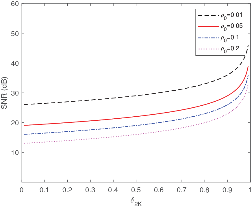
For any constant ρ0∈(0,1)\rho_{0}\in(0,1), if s​n​r≥C1ρ0snr\geq\frac{C_{1}}{\rho_{0}}, where C1=1δ​(1−δ)2C_{1}=\frac{1}{{\delta}(1-\delta)^{2}} is a constant, OMP recovers the support of KK-sparse signal 𝐱\mathbf{x} from its noisy measurements 𝐲=𝚽​𝐱+𝐯\mathbf{y}=\mathbf{\Phi x}+\mathbf{v} with error rate ρerror≤ρ0\rho_{\text{error}}\leq\rho_{0}.

Fig. 1 depicts the functional relationship between the required s​n​rsnr and δ\delta for different ρ0\rho_{0}.

Moreover, we would like to mention two major points of our proof that differ to those in [16].

  1. i)

    We fix τ\tau so that τ​K\tau K is an integer (e.g., τ=1\tau=1 simply meets the condition). By doing so, we can write ⌈τ​K⌉\lceil\tau K\rceil as τ​K\tau K, which can largely simplify the proof. In fact, we can fix τ\tau, θ1\theta_{1} and θ2\theta_{2} to any value in their feasible domain to promote our proof. Since 0<θ1<10<\theta_{1}<1 and θ2>0\theta_{2}>0, for any given δ\delta and fixed τ\tau, we can fix θ1\theta_{1} and θ2\theta_{2} to make sure that C1C_{1} and is bounded. Whereas in [16], δ\delta was set to be δ12\delta^{\frac{1}{2}}, and θ1\theta_{1} was fixed to θ\theta, which are clearly not optimal.

  2. ii)

    Our results are given in terms of m​a​rmar, while having no dependence on xm​a​xx_{max} (i.e., the element of maximum magnitude in the signal 𝐱\mathbf{x}). The key idea that allows to do so is that we replace all ‖𝐯‖22\|\mathbf{v}\|_{2}^{2} with ‖𝚽​𝐱‖22s​n​r\frac{\|\mathbf{\Phi x}\|_{2}^{2}}{snr} and bound ‖𝚽​𝐱‖22\|\mathbf{\Phi x}\|_{2}^{2} with the RIP. While in the [16], ‖𝐯‖22\|\mathbf{v}\|_{2}^{2} is bounded by the inequality

    2τ​‖𝐯‖22⩽2​τ2​(1+τ2)​K​(xm​i​n)2,\displaystyle\frac{2}{\tau}\|\mathbf{v}\|_{2}^{2}\leqslant 2\tau^{2}(1+\tau^{2})K(x_{min})^{2},

    so that some ‖𝚽​𝐱‖22\|\mathbf{\Phi x}\|_{2}^{2} has to be upper bounded by (1+δ)​K​(xm​a​x)2(1+\delta)K(x_{max})^{2}, which inevitably causes loosening in the subsequent analysis.

Refer to caption
Fig. 1: The required s​n​rsnr as a function of δ2​K\delta_{2K}
Refer to caption
Fig. 2: The required s​n​rsnr as a function of δ2​K\delta_{2K}

III-B Best achievable bound

To reach the best achievable result, we minimize C1C_{1} in (13). As C1=1(1−θ1)​(1−δ)​[1θ1+1θ2+(1−τ)​(1+δ)τ2]C_{1}=\frac{1}{(1-\theta_{1})(1-\delta)}[\frac{1}{\theta_{1}}+\frac{1}{\theta_{2}}+\frac{(1-\tau)(1+\delta)}{\tau^{2}}], fix θ1=12\theta_{1}=\frac{1}{2}, τ=1\tau=1, θ2→∞\theta_{2}\rightarrow\infty (1δ⁡(1−δ)\frac{1}{\delta(1-\delta)} takes the minimum value when δ=12\delta=\frac{1}{2}) so that C1=4(1−δ)C_{1}=\frac{4}{(1-\delta)}. In the case that m​a​r=1mar=1, we have the following corollary.

Corollary 3.

For any constant ρ0∈(0,1)\rho_{0}\in(0,1), if s​n​r≥C1ρ0snr\geq\frac{C_{1}}{\rho_{0}}, where C1=4(1−δ)C_{1}=\frac{4}{(1-\delta)} is a constant, OMP recovers the support of KK-sparse signal 𝐱\mathbf{x} from its noisy measurements 𝐲=𝚽​𝐱+𝐯\mathbf{y}=\mathbf{\Phi x}+\mathbf{v} with error rate ρerror≤ρ0\rho_{\text{error}}\leq\rho_{0}.

In Fig. 2, we plot the functional relationship between the required s​n​rsnr and δ\delta for different ρ0\rho_{0}.

III-C Bounds on SNR and Sampling Rate

Fix C1=4(1−δ)C_{1}=\frac{4}{(1-\delta)}. Then, for any small error value ρ0\rho_{0} we wish to achieve (i.e., ρerror=ρ0\rho_{\text{error}}=\rho_{0}), it should satisfy that

s​n​r≥4ρ0​(1−δ)​m​a​r.\displaystyle snr\geq\frac{4}{\rho_{0}(1-\delta)mar}. (15)

From [3, Equation (3)] we have known that for any asymptotically reliable recovery must meet the conditions that:

mn≥h⁡(Kn)−h⁡(Kn,ρ0)+1n​I​(x;y|K)12​log⁡(1+s​n​r)\displaystyle\frac{m}{n}\geq\frac{h(\frac{K}{n})-h(\frac{K}{n},\rho_{0})+\frac{1}{n}I(x;y|K)}{\frac{1}{2}{\log}(1+snr)} (16)

where h⁡(x)=−x​log​(x)−(1−x)​log​(1−x)h(x)=-x\textsl{log}(x)-(1-x)\textsl{log}(1-x) is the binary entropy function with

h⁡(x,y)=x​h​(y)+(1−x)​h​(y1x−1),\displaystyle h(x,y)=xh(y)+(1-x)h\left(\frac{y}{\frac{1}{x}-1}\right), (17)

and I⁡(x;y|K)I(x;y|K) is mutual information between x and y conditioned on KK, mn\frac{m}{n} is the sampling rate. The conditional mutual information I⁡(x;y|K)I(x;y|K) is zero for non-stochastic signals, so the condition becomes

s​n​r≥e2​nm​(h⁡(Kn)−h⁡(Kn,ρ0)CLOSE−1\displaystyle snr\geq e^{\frac{2n}{m}(h(\frac{K}{n})-h(\frac{K}{n},\rho_{0})}-1 (18)

To ensure an asymptotically reliable recovery, ρ0\rho_{0} should obey

4ρ0​(1−δ)​m​a​r≥e2​nm​(h⁡(Kn)−h⁡(Kn,ρ0)CLOSE−1.\displaystyle\frac{4}{\rho_{0}(1-\delta)mar}\geq e^{\frac{2n}{m}(h(\frac{K}{n})-h(\frac{K}{n},\rho_{0})}-1. (19)

Since 4ρ0​(1−δ)⋅MAR>4ρ0,\frac{4}{\rho_{0}(1-\delta)\cdot\text{MAR}}>\frac{4}{\rho_{0}}, which is because δ∈(0,1)\delta\in(0,1) and m​a​r≤1mar\leq 1 and e2​nm​(h⁡(Kn)−h⁡(Kn,ρ0)CLOSE−1≤e2​nm​(h​(Kn)CLOSE−1e^{\frac{2n}{m}(h(\frac{K}{n})-h(\frac{K}{n},\rho_{0})}-1\leq e^{\frac{2n}{m}(h(\frac{K}{n})}-1, (19) can be guaranteed whenever

ρ0≤4e2​nm​h​(Kn)−1.\displaystyle\rho_{0}\leq\frac{4}{e^{\frac{2n}{m}h(\frac{K}{n})}-1}. (20)

As ρ0<1\rho_{0}<1, this can be easily achieved by sparse signals for which Kn\frac{K}{n} is small enough.

On the other hand, from [3, Equation (9)], we have known that an asymptotically reliable recovery is promised when the following inequalities hold:

{s​n​r⋅ρ0≥e,mn>Kn+2​h​(Kn)log​(s​n​r⋅ρ0/e).\begin{cases}snr\cdot\rho_{0}\geq e,\\ \frac{m}{n}>\frac{K}{n}+\frac{2h(\frac{K}{n})}{\textsl{log}(snr\cdot\rho_{0}/e)}.\end{cases} (21)

Since δ∈(0,1)\delta\in(0,1) and m​a​r≤1mar\leq 1, the first inequality in (21) can be ensured by (15). Also, the second inequality of (21) shows that if the sampling rate mn\frac{m}{n} is fixed, it should be obeyed that

s​n​r⋅ρ0>e2​n⋅h⁡(Kn)m−K+1.\displaystyle snr\cdot\rho_{0}>e^{\frac{2n\cdot h(\frac{K}{n})}{m-K}+1}. (22)

To get the second inequality of (21) from (15), we should have

4ρ0​(1−δ)​m​a​r≥1ρ0​e2​n⋅h⁡(Kn)m−K+1\displaystyle\frac{4}{\rho_{0}(1-\delta)mar}\geq\frac{1}{\rho_{0}}e^{\frac{2n\cdot h(\frac{K}{n})}{m-K}+1} (23)

Similarly, it can be guaranteed if 4ρ0≥1ρ0​e2​n⋅h⁡(Kn)m−K+1,\frac{4}{\rho_{0}}\geq\frac{1}{\rho_{0}}e^{\frac{2n\cdot h(\frac{K}{n})}{m-K}+1}, or equivalently,

e2​n⋅h⁡(Kn)m−K+1<4.\displaystyle e^{\frac{2n\cdot h(\frac{K}{n})}{m-K}+1}<4. (24)

Again, this can be easily achieved by sparse signals with Kn\frac{K}{n} being small enough. Therefore, we can safely conclude that our results apply for asymptotically reliable recovery with achievable sampling rate.

IV Conclusion

In this paper, we have derived a new bound on the SNR for approximate support recovery via OMP. Our result improves upon that in [16], while offering an affirmative answer to conjecture of whether one can remove the dependence of xm​a​xx_{max} from the bound of SNR [16]. In practice, our result indicates more stable evaluation about the SNR and error rate, especially when the signal of interest is mixed by impulse-like wave (e.g., a impulse wave mixed by some minute noise) whose maxi,j∈supp​(𝐱)⁡|xi||xj|\max_{i,j\in\text{supp}(\mathbf{x})}\frac{|x_{i}|}{|x_{j}|} is unbounded from above.

References

  • [1] E. J. Candès and T. Tao, “Decoding by linear programming,” IEEE Trans. Inform. Theory, vol. 51, no. 12, pp. 4203–4215, Dec. 2005.
  • [2] D. L. Donoho, “Compressed sensing,” IEEE Trans. Inform. Theory, vol. 52, no. 4, pp. 1289–1306, Apr. 2006.
  • [3] G. Reeves and M. Gastpar, “Sampling bounds for sparse support recovery in the presence of noise,” IEEE International Symposium on Information Theory, pp. 2187-2191, July. 2008.
  • [4] G. Tang and A. Nehorai, “Performance analysis for sparse support recovery,” IEEE Trans. Inform. Theory, vol. 56, no. 3, pp. 1383-1399, 2010.
  • [5] B. K. Natarajan, “Sparse approximate solutions to linear systems,” SIAM journal on computing, vol. 24, no. 2, pp. 227–234, Apr. 1995.
  • [6] Y. C. Pati, R. Rezaiifar, and P. S. Krishnaprasad, “Orthogonal matching pursuit: Recursive function approximation with applications to wavelet decomposition,” in Proc. 27th Annu. Asilomar Conf. Signals, Systems, and Computers. IEEE, Nov. Pacific Grove, CA, Nov. 1993, vol. 1, pp. 40–44.
  • [7] T. Zhang, “On the consistency of feature selection using greedy least squares regression,” J. of Mach. Learn. Res., vol. 10, pp. 555–568, 2009.
  • [8] J. A. Tropp and A. C. Gilbert, “Signal recovery from random measurements via orthogonal matching pursuit,” IEEE Trans. Inform. Theory, vol. 53, no. 12, pp. 4655–4666, Dec. 2007.
  • [9] M. A. Davenport and M. B. Wakin, “Analysis of Orthogonal Matching Pursuit using the restricted isometry property,” IEEE Trans. Inform. Theory, vol. 56, no. 9, pp. 4395–4401, Sep. 2010.
  • [10] E. Liu and V. N. Temlyakov, “The orthogonal super greedy algorithm and applications in compressed sensing,” IEEE Trans. Inform. Theory, vol. 58, no. 4, pp. 2040–2047, Apr. 2012.
  • [11] E. D. Livshits, “On the efficiency of the orthogonal matching pursuit in compressed sensing,” Sbornik: Mathematics, vol. 203, no. 2, pp. 183, 2012.
  • [12] Q. Mo and Y. Shen, “A remark on the restricted isometry property in orthogonal matching pursuit algorithm,” IEEE Trans. Inform. Theory, vol. 58, no. 6, pp. 3654–3656, Jun. 2012.
  • [13] J. Wang and B. Shim, “On the recovery limit of sparse signals using orthogonal matching pursuit,” IEEE Trans. Signal Process., vol. 60, no. 9, pp. 4973–4976, Sep. 2012.
  • [14] C. Soussen, R. Gribonval, J. Idier, and C. Herzet, “Joint kk-step analysis of orthogonal matching pursuit and orthogonal least squares,” IEEE Trans. Inform. Theory, vol. 59, no. 5, pp. 3158–3174, May 2013.
  • [15] L. Chang and J. Wu, “An improved RIP-based performance guarantee for sparse signal recovery via orthogonal matching pursuit,” IEEE Trans. Inform. Theory, vol. 60, no. 9, pp. 5702–5715, Sep. 2014.
  • [16] J. Wang “Support recovery with orthogonal matching pursuit in the presence of noise: A new analysis,” IEEE Transactions on Signal processing, vol. 63, no. 21, pp. 5868–5877, Jan. 2015.
  • [17] R. Wu, W. Huang, and D Chen, “The exact support recovery of sparse signals with noise via orthogonal matching pursuit,” IEEE Signal Processing Letters, vol. 20, no. 4, pp. 403–406, Apr. 2013.
  • [18] J. Wen, Z. Zhou, J. Wang, X. Tang and Q. Mo, “ A sharp condition for exact support recovery with orthogonal matching pursuit,” IEEE Transactions on Signal Processing, vol. 65, no. 6, pp. 1370–1382, 2016.
  • [19] E. D. Livshitz and V. N. Temlyakov, “Sparse approximation and recovery by greedy algorithms,” IEEE Trans. Inform. Theory, vol. 60, no. 7, pp. 3989–4000, Jul. 2014.