Fairness-Oriented Multiple RIS-Aided mmWave Transmission: Stochastic Optimization Methods
Abstract
In millimeter wave (mmWave) systems, it is challenging to ensure the reliable connectivity of communication due to the high sensitivity to the presence of blockages. In order to improve the robustness of mmWave systems under the presence of random blockages, multiple reconfigurable intelligent surfaces (RISs) are deployed to enhance the spatial diversity gain, and robust beamforming is then designed based on a stochastic optimization for minimizing the maximum outage probability among multiple users to ensure fairness. Under the stochastic optimization framework, we adopt the stochastic majorization–minimization (SMM) method and the stochastic successive convex approximation (SSCA) method to construct deterministic surrogate problems at each iteration for new channel realizations, and to obtain closed-form solutions of the precoding matrix at the base station (BS) and the passive beamforming vectors at the RISs. Both stochastic optimization methods are proved to converge to the set of stationary points of the original stochastic problems. Finally, simulation results show that the proposed robust beamforming in RIS-aided systems can effectively compensate for the performance loss caused by the presence of random blockages, especially when the blockage probability is high, compared with benchmark solutions.
Index Terms:
Reconfigurable intelligent surface (RIS), intelligent reflecting surface (IRS), millimeter wave communications, stochastic optimization, robust beamforming design.I Introduction
Millimeter wave (mmWave) communication is expected to be a promising technology to meet the growing demand for data rate in current and future wireless networks due to the abundant spectrum available at high frequencies. High frequency communication inevitably has severe attenuation, but this can be compensated by an array of reasonable size containing a large number of antennas due to the small wavelength [1]. In addition, the high-directional beams of large arrays are capable of mitigating the inter-user interference. However, mmWave communication systems suffer from high penetration loss [2, 3, 4]. Hence, mmWave systems are much more susceptible to the presence of spatial blockages than sub-6 GHz systems, and the reliability of the communication links for the entire network cannot always be guaranteed [2, 3, 4].
In particular, spatial blockages can be divided into static blockages (e.g., buildings and other immobile fixtures), dynamic blockages (e.g., humans, vehicles, or moving obstructions) and self-blockages (e.g., hand blocking of the user itself and blockage from other body parts). Some statistical models are established to characterize the properties of the random dynamic blockages and self-blockages [5, 3, 4]. The authors of [6] have developed a distance-dependent blockage probability model, in which the probability of link blocking increases exponentially with the link length. Furthermore, [7] and [8] proposed a mechanism to predict the blockage probability via machine learning. When the blockage probability is obtained, some robust beamforming design strategies have been proposed in the recent literature [9, 10] to address channel uncertainties caused by the presence of random blockages. Specifically, the authors of [9] proposed a worst-case robust beamforming design for application to coordinated multipoint (CoMP) systems in which all possible combinations of blockage patterns were considered. Due to the high computational complexity of the ergodic method in [9], an outage-minimum strategy based on a stochastic optimization method was proposed for CoMP systems in [10] to improve the robustness of mmWave systems. The idea of adopting multiple base stations (BSs) in CoMP systems is effective to compensate for the performance loss caused by the presence of random blockages by exploiting spatial diversity gains. However, this will incur excessive hardware cost and power consumption. Another promising scheme proposed in [11] is to deploy cost-efficient reconfigurable intelligent surfaces (RISs) in mmWave systems to create an alternative communication link via the RISs.
Due to the promising advantages in terms of providing energy- and spectral-efficient communications, RISs have attracted extensive research attention from both academia and industry [12, 13, 14, 15]. An RIS is a thin surface consisting of nearly-passive and reconfigurable reflecting elements, which reflects the impinging radio waves without adopting radio frequency (RF) chains. The passive elements on the RIS can be tuned to alter their electromagnetic response such that the signals reflected from an RIS can be constructively superimposed to enhance the signal power at the intended receiver or destructively combined to avoid the information leakage to undesired receivers. These characteristics make RISs appealing to be applied in various communication systems as shown in [16]. For instance, RISs can be applied in single-cell multiple-input and multiple-output (MIMO) systems [17, 18, 19, 20, 21], multicell MIMO communications [22], simultaneous wireless information and power transfer (SWIPT) systems [17, 23], secure communications [24], mmWave systems [25, 26, 27, 28] and THz systems [29, 30].
Although the performance advantages of deploying an RIS in mmWave systems have been demonstrated in recent contributions, there still exist major open problems to solve. The authors of [26] only considered the BS-RIS-user channels and assumed that the direct BS-user communication links were completely blocked by obstacles. However, this assumption only applies to the case of static blockages with outage probability of 1, but not to the case of dynamic blockage with outage probability varying between 0 and 1 [2, 3, 4]. The numerical results in [27] showed that the gain from additional reflection channels could compensate for the performance loss caused by the presence of random blockages, but the impact of blockages was not considered in the beamforming design. Most recently, we have considered the robust beamforming design for RIS-aided mmWave communication systems in [11] by taking the random blockages into consideration. However, the objective function therein is to minimize the sum outage probability, which cannot ensure the fairness for all the users.
I-A Novelty and contributions
Against the above background, this paper proposes a robust transmission strategy in an RIS-aided mmWave communication system to deal with the channel uncertainties caused by the random blockages while ensuring the fairness among the users. Some common approaches to handle the imperfect and partial CSI problem are the outage constrained robust optimization and the worst-case robust optimization techniques [31]. However, both of them still need the estimation of the instantaneous CSI, and the worst-case robust method is conservative and hence suboptimal due to the low probability of occurrence for the worst case. An alternative approach is to design the robust beamforming by optimizing the statistical performance under a stochastic optimization framework in which only the long-term CSI is required. In what follows, we propose a maximum outage probability minimization problem to be solved by using the stochastic optimization framework.
Specifically, the main contributions of this work are summarized as follows:
- •
To the best of our knowledge, this is the first work exploring the robust beamforming design for an RIS-aided downlink multiuser mmWave system with the knowledge of long-term CSI and blockage probability. Specifically, our optimization objective in this work is to minimize the maximum outage probability of all the users. Different from the sum outage probability minimization problem in [10, 11], the min-max outage probability objective can ensure the quality of service (QoS) performance for the worst-case user in the downlink multiuser system. Due to the non-differentiable objective function, the stochastic gradient descent (SGD) method adopted in [10, 11] cannot be directly applied. To resolve this problem, two more general and powerful stochastic optimization frameworks are adopted to jointly optimize the active precoding at the BS and the passive beamforming at the RISs.
- •
The single user case is firstly considered to obtain insights for the robust beamforming design by minimizing the outage probability in the presence of long-term CSI and random blockages. Due to the non-deterministic expression of the probability function in the objective function, we replace it with an expectation function over the long-term CSI and blockage probability. Then, the inner step function in the expectation is approximated by a smooth function which is twice differentiable for the precoding at the BS and the passive beamforming at the RISs, respectively. The resulting expectation optimization problem is solved by adopting the stochastic majorization–minimization (SMM) method in which an upper bound surrogate function of the original differentiable function is constructed for a new channel realization at each iteration. The constructed surrogate problem has closed-form solutions and is computationally efficient. We prove that the proposed SMM method is guaranteed to converge to the set of stationary points of the original expectation minimization problem.
- •
The robust beamforming for a more general multiuser case is designed by solving a maximum outage probability minimization problem. To tackle the non-differentiability of the max objective function, we firstly replace it with its log-sum-exp upper bound. The stochastic successive convex approximation (SSCA) method is then adopted, which has more flexibility in the choice of the surrogate function than the SMM method, and generates closed-form solutions at each iteration. Furthermore, we prove that the final solution generated by the iterative algorithm is guaranteed to converge to the stationary point of the original expectation minimization problem.
- •
We demonstrate through numerical results that the proposed robust beamforming algorithm outperforms its non-robust counterpart and the robust beamforming in conventional RIS-free systems both in terms of maximum outage probability and minimum effective rate if the blockage probability is high. Moreover, deploying multiple small-size RISs is shown to be more effective than deploying a single large-size RIS in terms of improving the performance of the worst-case user.
The remainder of this paper is organized as follows. Section II introduces the system model. The outage probability minimization problem is formulated for a single-user case in Section III. Section IV further investigates the min-max outage probability problem for the multiuser system. Finally, Sections VI and VII report the numerical results and conclusions, respectively.
Notations: The following mathematical notations and symbols are used throughout this paper. Vectors and matrices are denoted by boldface lowercase letters and boldface uppercase letters, respectively. The symbols , , , and denote the conjugate, transpose, Hermitian (conjugate transpose), Frobenius norm of matrix , respectively. The symbol denotes 2-norm of vector . The symbols , , , , and denote the trace, real part, modulus, eigenvalue, and angle of a complex number, respectively. is a diagonal matrix with the entries of on its main diagonal. means the -th element of the vector . The Kronecker product between two matrices and is denoted by . means that is positive semidefinite. Additionally, the symbol denotes complex field, represents real field, and is the imaginary unit. The inner product is defined as
II System Model
II-A Signal Model

As shown in Fig. 1, we consider an RIS-aided downlink mmWave communication system. In order to ensure high QoS for the users in the presence of random blockages, RISs, each of which has passive antennas, are deployed to assist the communication from the BS equipped with active antennas to single-antenna users (denoted by ). The RISs are assumed to be connected to controllers that exchange control information with the BS through dedicated channels [17, 22]. The baseband transmitted signal at the BS is , where is the Gaussian data symbol vector and denotes the full-digital beamforming matrix. The baseband transmit power is limited to the total transmit power . Hence, belongs to the set .
Let , and denote the channels of the BS-user , BS-RIS , and RIS -user links, respectively. Then, the received signal intended to the -th user is expressed as
| (1) |
where is the additive white Gaussian noise (AWGN), and is the reflection coefficient matrix (also known as the passive beamforming matrix) of the -th RIS. Element is the unit modulus coefficient of the -th phase shift at the -th RIS, and indicates the reflection efficiency. Here, it is assumed that for investigation of the performance upper bound of RIS.
Furthermore, after defining the compact matrices and , we obtain the equivalent channel between the BS and the -th user. The corresponding equivalent reflection coefficient vector is given by which belongs to the set . Then, (1) can be rewritten into a compact form as
| (2) |
and the corresponding achievable signal-to-interference-plus-noise ratio (SINR) is
| (3) |
II-B Channel Model
It is important to mention that the perfect instantaneous CSI of a mmWave system is difficult to obtain due to the passive implementation of the RIS reflecting elements. More specifically, estimating the full instantaneous CSI for all links would inevitably require a large training overhead. In this work, since the channel modeling of the RIS-related links is the same as the traditional wireless channel modeling [32], we adopt a Saleh-Valenzuela (SV) channel model [33] to characterize the mmWave channels where only the large-scale fading characteristics is required during the transmission design. In particular, it is assumed that the uniform planar array (UPA) is deployed on the BS and each RIS. The steering vector of the UPA is in which denotes the azimuth (elevation) AoD and the angle-of-arrival (AoA) of the transceivers. We assume that there are , and sparse scatterers for the BS-user , the RIS -user and the BS-RIS links, respectively, and each of the scatterers comprises subpaths. Thus, the mmWave channels can be expressed as
| (4) | ||||
| (5) | ||||
| (6) |
where, by denoting an arbitrary element , then is the line-of-sight (LoS) component with fading coefficient following the distribution , where is the power fraction that corresponds to the Rician factor , and is the distance-dependent large-scale fading model. The remaining paths are the line-of-sight (NLoS) components whose fading coefficients follow the distribution with power fraction .
We assume that the user’s locations are quasi-static over milliseconds or even seconds. Therefore, the large-scale fading characteristic parameters, such as the distance-dependent path loss, the numbers of clusters, their power fraction, the cluster central angles and angular beamspreads, change relatively slowly [34] and can be perfectly known by the BS. However, the instantaneous CSI, given by 11 1 With the knowledge of long-term large-scale fading characteristic parameters, each sample of can be obtained by generating , AoDs and AoAs according to their Gaussian distribution., vary during the transmission due to the rapidly varying small-scale fading coefficients , AoDs and AoAs according to an ergodic stationary process. These AoDs and AoAs can be generated according to a Gaussian distribution, whose expectation values are the cluster central angles and variance values are the angular spreads [34].
Based on the fact that the communication links in the mmWave frequency band are sensitive to the presence of blockages, most existing contributions considered a worst-case scenario where the BS-user links are completely blocked by the obstacles during the whole transmission, while the RIS-related links are not affected by blockages since the locations of the RISs can be appropriately chosen to ensure line-of-sight transmission. However, this assumption may be impractical in many scenarios. Traditionally, blockage effects are incorporated into the shadowing model, along with reflections, scattering, and diffraction [5]. In contrast, we adopt a recently proposed probabilistic model [10] to characterize the channel uncertainties caused by the presence of random blockages. In particular, by introducing the blockage parameters , which are random variables following a Bernoulli distribution with a blockage probability of , the channels in (4) for the BS-user links are modified to
| (7) |
Analytical results show that the probability of link blocking increases exponentially with the link length [5], thus we adopt a distance-dependent blockage probability model given by , where physical distance parameter between the BS and user can be extracted from the estimated CSI by the BS, and parameters and are fit from the data [6].
II-C Problem Formulation
To account for the presence of random blockages and to enhance the QoS of the users, we design a robust beamforming by minimizing the maximum outage probability among all users over the random CSI. The formulated optimization problem is given by
| (8a) | ||||
| s.t. | (8b) | |||
| (8c) | ||||
where the outage probability is the probability that the SINR of the user is less than the SINR reliability threshold for all possible realizations of the random channel .
III Single-User System
In this section, we consider a single-user system model in order to obtain some design insights. By setting and dropping the user index, Problem (8) is simplified to
| (9a) | ||||
| s.t. | (9b) | |||
| (9c) | ||||
III-A Problem Reformulation
The probability has no closed-form expression and thus the problem in (9) is prohibitively challenging to be solved directly. An alternative solution is to replace the probability function with an equivalent expectation function, i.e., where is the step function of the event . By doing so, various stochastic programming techniques can be used. However, the step function is discontinuous, and the existing stochastic programming methods cannot be directly applied.
To resolve this issue, we approximate the step function with a smooth approximating function
| (10) |
where and is the smooth parameter controlling the approximation error.
By defining , a convenient approximation of Problem (9) is
| (11) |
III-B Stochastic Majorization-Minimization Method
A simple approach for solving the above problem is the sample average approximation (SAA) method. However, the SAA method is computationally prohibitive since it requires large-sized memory storage due to the fact that the solution obtained at each iteration is calculated by averaging over a large number of channel realizations. To overcome these difficulties, we adopt the widely used SMM [35] (also known as stochastic successive minimization [36]) method in which a well-chosen upper bound approximation of the function for a new channel sample is constructed at each iteration and the solution is obtained on the average of the new channel sample and the others generated in previous iterations.
The standard of constructing the upper bound approximation function of is to make the corresponding surrogate problem easy to solve and even obtain the closed-form solutions. In particular, denote that belongs to }, the surrogate function of around any feasible point needs to satisfy the following assumptions [36].
Assumption A
defines the directional derivative of in the direction and is given by
The Assumptions (A2)-(A3) indicate that the surrogate function is a locally upper bound of the original function around the feasible point . Assumption (A4) is a derivative consistency condition. To ensure the convergence of the SMM algorithm, we further make the following assumptions [36].
Assumption B
| derivatives are uniformly bounded. |
Since the variables and are highly coupled with each other, we adopt an alternating optimization (AO) method to update them. Based on the above assumptions, the variables and are updated by solving the following two SMM subproblems:
| (12) |
and
| (13) |
Here, are some independent samples of the random equivalent channel . is a surrogate function corresponding to when is given, while is the corresponding surrogate function of with given .
III-B1 Optimizing
First, we construct satisfying Assumptions A and B, which is shown in the following lemma.
Lemma 1
For the twice differentiable function , we construct its second-order upper bound approximation around any fixed , which is given by
| (14) |
where
| (15a) | ||||
| (15b) | ||||
| (15c) | ||||
| (15d) | ||||
| (15e) | ||||
Proof: See Appendix A.
By using (14) and ignoring constants, the subproblem in (12) for updating is formulated as
| (16) |
Problem (16) is convex and can be solved by computing its Lagrange function given by
| (17) |
where is a Lagrange multiplier associated with the power constraint. By setting , the globally optimal solution of at the -th iteration is derived as
| (18) |
Also, (18) must satisfy the power constraint, which yields
| (19) |
Based on the fact that the left hand side of (19) is a decreasing function of , we obtain the following closed-form solution
| (20) |
The first option in (20) is based on . The second option is due to the fact that there must exist a that (19) holds with equality.
III-B2 Optimizing
As for the update of with given , we first construct a surrogate function corresponding to in the following lemma.
Lemma 2
For the twice differentiable function , we construct its second-order upper bound approximation around any feasible , which is given by
| (21) |
where
| (22a) | ||||
| (22b) | ||||
| (22c) | ||||
| (22d) | ||||
By substituting (21) into the objective function of subproblem (13) and ignoring constants, we obtain:
| (23) |
The globally optimal solution of the above problem is given by
| (24) |
where means the -th element of vector, is the imaginary unit, denotes the angle of a complex number, and is an element-wise operation.
III-C Algorithm Development
Under the SMM framework, closed-form solutions of in (20) and of in (24) at each iteration are obtained. Such simple closed-form solutions can greatly reduce the computational complexity. Algorithm 1 summarizes the proposed robust beamforming design based on the SMM-based outage probability minimum problem for RIS-aided single-user mmWave systems in which the BS-user links experience random blockages. The proposed algorithm is referred to as SMM-OutMin. Note that the convergence speed of the SMM-based algorithm might be affected by the tightness of the upper bounds in Lemma 1 and Lemma 2, thus SQUAREM [37] is adopted to accelerate the SMM-based algorithm. Denote by and the objective function values of Problem (16) and Problem (23) in the -th iteration, respectively. is an operation mapped to nonlinear constraint set. For the power constraint set , can be . For the unit-modulus constraint set , can be element-wise operation, i.e., . Steps 10 to 13 and steps 21 to 24 are used to maintain the convergence property of the objective function values.
III-C1 Convergence analysis
The convergence of Algorithm 1 is given in the following theorem.
Theorem 1
Proof: See Appendix B.
III-C2 Complexity analysis
IV Multiuser System
In this section, we consider the general multiuser setup and solve Problem (8). Problem (8) is more challenging than problem (9) due to the non-differentiable objective function. Furthermore, the complex objective function complicates the use of the SMM algorithm, thus we extend the SMM method to a general algorithm to solve Problem (8).
IV-A Problem Reformulation
We first approximate the probability function in the original Problem (8) by using the expectation of the smooth function in (10). By defining , in which is a diagonal matrix whose diagonal entry is except in the -th diagonal element that is , the approximate objective function is . However, the obtained function is still intractable since the maximization operation couples and the different channel states due to the expectation operation. This issue motivates us to use the following Jensen inequality
| (25) |
due to the fact that the max function is convex [38].
Furthermore, the non-differentiable max function, , is approximated by adopting a smooth log–sum–exp upper-bound [39]
| (26) |
where is a smoothing parameter satisfying
| (27) |
When is chosen appropriately, the smooth approximation of Problem (8) is approximately reformulated as
| (28) |
IV-B Stochastic Successive Convex Approximation Method
Similar to Problem (11), Problem (28) can still be solved by adopting the SMM method. However, the function in (26) is much more complex and its second-order derivative, which is necessary to construct the upper bound surrogate function of as shown in Appendix A, is not easy to be calculated. Furthermore, the coefficient of the second-order term in the final upper-bound surrogate function of ( in (14)) can be quite loose, resulting in a very slow convergence rate of the SMM algorithm.
Therefore, in this section, we adopt a flexible SSCA method to address the above issues. The surrogate functions employed by the SSCA method do not need to be an upper bound of the original function but they need only to preserve the first-order property of the original function. Accordingly, the surrogate functions need to satisfy Assumption B and the following assumptions [40].
Assumption C
Assumption C cannot ensure that the sequences of the approximate objective values are monotonically decreasing at each iteration. Nevertheless, to guarantee convergence, the variables can be updated by choosing an appropriate step size at each iteration that yields a sufficient decrease of the objective value. Based on the above assumptions, we choose the proximal gradient-like approximation to construct the surrogate function, which is
| (29) |
where can be any positive number.
IV-B1 Optimizing
The parameters in (30) are as follows
| (31a) | ||||
| (31b) | ||||
| (31c) | ||||
| (31d) | ||||
| (31e) | ||||
IV-B2 Optimizing
Furthermore, with fixed , the subproblem of Problem (28) corresponding to at the -th iteration is
| (34) |
where , and
| (35a) | ||||
| (35b) | ||||
| (35c) | ||||
Finally, the minimizer of Problem (34) is
| (36) |
IV-C Algorithm development
The simple closed-form solutions of in (33) and of in (36) can greatly reduce the computational complexity. Algorithm 2 summarizes the proposed SSCA-based robust beamforming design for RIS-aided multiuser mmWave systems in which the BS-user links experience random blockages. The proposed algorithm is referred to as SSCA-OutMin.
IV-C1 Step-size selection
It is worth noting that the approximation in (30) has the same form as that in (14). However, in the SSCA method can be any positive number, and might no longer be a global upper bound of . In this case, the step sizes and need to be carefully chosen to ensure convergence.
As an example, we take to illustrate the update rule, which is a line-search (also called Armijo step-size) rule: Consider and . Let be the largest element in such that
| (37) |
Theorem 2
If is chosen according to the line-search rule, then
Proof: See Theorem 7 in [41].
IV-C2 Convergence analysis
The convergence of Algorithm 2 is given in the following theorem.
Theorem 3
Proof: See Appendix C.
IV-C3 Complexity analysis
IV-C4 Initial point
Problem (28) has, in general, multiple local minima points due to the non-convex unit-modulus constraint and . The accurate selection of the initial points in Algorithm 2 plays an important role for the convergence speed and the quality of the obtained local solution. To that end, we first initialize to maximize the minimum equivalent total channel gain, resulting in the following optimization problem
| (38) |
Problem (38) can be efficiently solved by using the SDR method as follows
| (39a) | ||||
| s.t. | (39b) | |||
| (39c) | ||||
where and is an auxiliary variable.
Furthermore, is initialized by using the maximum-ratio transmission (MRT) method as
| (40) |
V Numerical results and discussion
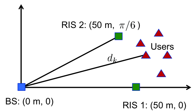
V-A Simulation setup
In this section, we numerically evaluate the performance of the proposed algorithms. All experiments are performed on a PC with a 1.99 GHz i7-8550U CPU and 16 GB RAM. We adopt a polar coordinate to describe the simulated system setup as shown in Fig. 2, where the BS is located at (0 m, 0), and the two RISs are deployed in the locations (50 m, 0) and (50 m, ) which are close to the users. The users are randomly placed in a range with polar diameter [50 m, 80 m] and polar angle , where is used to calculate the distance-dependent blockage probability. The large-scale fading, reported in urban micro (UMi)-street canyon scenario [42], is modeled as in dB with link distance (in meters), path loss exponent , and log-normal shadowing where denotes the log-normal shadowing variance. The mmWave system operates on carrier frequency GHz and bandwidth 20 MHz. Since the macro-scattering environment between the BS and the users are complex, only NLoS clusters are assumed to exist in the BS-user links, i.e., the Rician factor is . The parameter settings in of NLoS are and dB [42]. In practice, the RISs can be installed such that the BS-RIS links and the RIS-user links are blockage-free. Thus, the channels in (5) and (6) contain only LoS cluster with a Rician factor . The parameters in of LoS are and dB according to [42]. Unless stated otherwise, we assume and . The transmit power limit of the BS is dBm and the noise power at each user is dBm. For simplicity, we consider an equal blockage probability, , and an equal target SINR, , which yields the target rate . The smooth parameters are chosen to be and .
To evaluate the performance of the proposed stochastic optimization algorithms, we consider the following benchmark schemes. 1) SMRT: In this scheme, the active precoding is updated by using stochastic maximum-ratio transmission (SMRT), that is . The passive beamforming is still updated by using the SMM or SSCA methods. 2) NoRIS: In this case, no RIS is employed and the optimal active precoding is obtained by using the SMM or SSCA methods. 3) No-robust: In this scheme, the beamforming is designed by using the SMM or SSCA methods by taking into account the random small-scale parameters while assuming . 4) Imperfect CSI: In this scheme, the beamforming is designed by using the SMM or SSCA methods based on the imperfect CSI of cluster central angles. In specific, we assume that the modulus of the cluster central angle estimation error is 0.01. 5) SAA: In this scheme, we generate 300 independent channel realizations in advance, the solutions at each iteration is the average over these 300 channel samples, and the surrogate function used at each iteration is obtained by adopting the MM or SCA methods. We take the beamforming design in the single-user case as an example. By modifying Problems (12) and (13), the beamforming designed by using the SAA-MM method is updated as follows
| (41) |
and
| (42) |
In order to demonstrate the robustness of the proposed algorithms, we consider two performance metrics: the outage probability and the effective rate. In particular, the outage probability of each user is calculated by averaging over 1000 independent channel realizations. The corresponding effective rate of the -th user is defined as if and otherwise.
V-B Convergence
Fig. 3 investigates the convergence behavior of the considered stochastic optimization algorithms. For comparison, we consider a single-user case containing RIS 1 in Fig. 2, and the other parameters are given in Fig. 3. In Fig. 3, the coordinate value on the y-axis is the objective value of Problem (16) or (32), and not the actual outage probability of the original problem. It is observed from Fig. 3 that the SMM and SSCA algorithms are characterized by an oscillatory convergence which depends on the random channel generations at each iteration. On the other hand, using 300 channel realizations for each iteration leads to the monotonic convergence of the SAA algorithm when adopting a monotonically decreasing surrogate function for each channel realization. Although the SAA algorithm requires the least number of iterations to converge, it is much more computationally demanding than the other two algorithms. This fact can be observed in Table I which compares the CPU time consumption of each iteration and total CPU time consumption of iteration convergence for the three considered algorithms. Theoretically, the computational complexity of each iteration of the SAA algorithm is 300 times higher than that of the SMM or SAA algorithms, because at each iteration of the SAA algorithm, each parameter needs to be calculated 300 times for all channel realizations.

| Algorithms | The CPU time (sec) per iteration | The CPU time (sec) |
|---|---|---|
| SMM | 0.0025 | 1.8750 |
| SSCA | 0.0042 | 4.6719 |
| SAA | 0.3557 | 20.9844 |
V-C Single-user system
We consider a single-user system containing RIS 1 in Fig. 2 with the target rate of bps/Hz. Fig. 4 illustrates the performance of different algorithms as a function of the blockage probability. First, it can be seen that SMM-based beamforming in the RIS-aided mmWave system of outperforms the NoRIS scheme when . The main reason is that the direct BS-user channel may be much stronger than the cascaded BS-RIS-user channel as the latter experiences the double path loss effect, which is significant if the path-loss is large. Therefore, when the blockage probability is small (), the BS tends to allocate the transmit power to the stronger direct path, thus reducing the contribution of the RIS to the system performance. However, by increasing the number of reflecting elements at the RIS to , our proposed SMM algorithm outperforms the NoRIS system in the whole blockage probability region (i.e., ). The reason is that the RIS-aided reflecting channels starts to compensate for the performance loss caused by the blockages when . In addition, it can be seen that the performance of the SMM-based beamforming is the same as that of the SAA-based beamforming. Last but not least, compared with the No-robust RIS-aided scenario and the scheme with imperfect CSI, the robust RIS beamforming can significantly compensate for the performance loss caused by the presence of random blockages.

Fig. 5 shows the impact of the size of the RIS and the size of the antenna array at the BS on the outage probability by using the SMM algorithm. It can be observed from Fig. 5(a) that when BS is equipped with antennas, the RIS plays a significant role in guaranteeing the desired user’s QoS and improving the system robustness with increased number of reflection elements (). In other words, a large-size RIS with can still reduce the outage probability to about 0.1, even if the direct channel is completely blocked. Finally in Fig. 5(b) we observe that increasing the number of transmit antennas () has the same ability to reduce the outage probability as increasing the number of reflection elements (), except when the direct channel is completely blocked.

V-D Multiuser system
In this section, we consider a multiuser system with users, in which the target rate is bps/Hz. As we can see from Fig. 6(a), compared with the No-robust RIS-aided scenario, the robust beamforming in the RIS-aided scheme in a multiuser system can efficiently improve the maximum outage probability. In addition, different from the single-user system of , the RIS-aided setup outperforms the NoRIS scheme only when . This fact is consistent with the observation of in Fig. 4 (a), that is, the performance gain of an RIS starts to manifest when . Further increasing the number of RISs and the size of each RIS can reduce the maximum outage probability in the whole blockage probability region (i.e., ). Although the improvement in the performance in terms of the maximum outage probability of the large-size RIS beamforming in Fig. 6(a) is slightly weak, the enhancement of the corresponding minimum effective rate shown in Fig. 6(b) is apparent. Specifically, the minimum effective rate of the robust designs is better than that of the non-robust schemes. Moreover, the contribution of the RIS in improving the minimum effective rate is also apparent for the almost blockage probability region (i.e., ). Finally, we observe that multiple RISs with a relatively small size can improve the worst-case user’s performance, and outperform the performance offered by a single RIS with large size, especially in the multi-user scenario. This is because the optimal deployment of multiple RISs can provide more spatial diversity for users who are far away from the RIS, thus improving the system performance.

Finally, Fig. 7 investigates the performance as a function of the number of users. For a fair comparison, we consider the setup and . Compared with the NoRIS scheme, the contribution of multiple RISs in reducing the maximum outage probability shown in Fig. 7 decreases as the increase of . When , the RIS scheme cannot guarantee the QoS performance of the worst-case user due to the high outage probability.
VI Conclusions
In this work, we have improved the reliability of a mmWave system in the presence of random blockages by employing multiple RISs and designing the corresponding robust beamforming. In order to reduce the system outage, we have formulated and solved a maximum outage probability minimization problem which belongs to the family of stochastic optimization problems . More precisely, we have taken into account the statistical CSI and the blockage probability, and have solved the formulated optimization problem by adopting a stochastic optimization framework. Closed-form solutions have been derived at each iteration by adopting the SMM and SSCA methods. The two proposed stochastic methods are guaranteed to converge to the set of stationary points of the original stochastic problems. Selected numerical results have demonstrated the performance gain in terms of outage probability and effective rate of the RIS-aided mmWave systems in the presence of random blockages.
Appendix A The proof of Lemma 1
In this subsection, is dropped for simplicity, i.e., is replaced by . Since is twice differentiable, we propose a second-order approximation to upper bound at any fixed point :
| (43) |
where and are to be designed to satisfy Assumption A.
Assumptions (A1) and (A2) are readily satisfied. Assumption (A4) is a derivative consistency condition. Denote , then the directional derivative of at with direction is
| (44) |
The corresponding directional derivative of is
| (45) |
where is given in (15c).
In order for Assumption (A3) to hold, it is sufficient to show that is an upper bound for each linear cut in any direction. In particular, let , we need to show
| (47) |
Define and . (47) holds if the second-order derivative of is no more than that of the right hand side of (47). The corresponding sufficient condition can be formulated as
| (48) |
Before deriving the expression of , we calculate the first-order derivative of , as follows
| (49) |
where , , and .
Then, the second-order derivative is derived as
| (50) |
where and .
Furthermore, we also manipulate the right hand side of (48) into the same form as in (A), as follows
Combining (A) and (A), the sufficient condition in (48) is equivalent to
which can be satisfied when satisfies
For convenience, we select . Then, in (43) is designed to be
where , and are defined in Lemma 1. The deterministic expression of is difficult to obtain, therefore we derive the upper bound shown as follows
The above inequalities are due to the following mathematical properties:
(p1): and are Hermitian matrices: [43].
(p2): is rank one: [43].
(p3): , where the equality holds when .
(p4): is positive semidefinite with maximum eigenvalue and is positive semidefinite: [43].
(p5): Power constraint: .
Hence, the proof is completed.
Appendix B The proof of Theorem 1
Define the random functions
| (61) | ||||
| (62) |
To state the convergence result, we need the following lemmas.
Lemma 3
Suppose Assumptions A and B are satisfied and define a limit point of a subsequence , then there exists uniformly continuous functions and such that
| (63) | ||||
| (64) | ||||
| (65) | ||||
| (66) |
Proof: First, it follows that is bounded for and all channel realizations due to the assumption (B2), and therefore, (63) holds by using the strong law of large numbers [44]. Also, the families of functions are equicontinuous and bounded over a compact set due to the assumption (B2) and the use of mean value theorem. Thus, by restricting to a subsequence, we have (64). Furthermore, the families of functions are also equicontinuous and bounded over a compact set due to the assumption (B2) that is bounded. Hence the Arzelà-Ascoli theorem [45] implies that, by restricting to a subsequence, there exists a uniformly continuous function such that (65) and (66) hold.
On the other hand, the update rule of Algorithm 1 leads the following lemma.
Lemma 4
, almost surely.
Proof: The proof of Lemma 4 is the same with that of ([36], Lemma 1) and is omitted for conciseness.
Then, (67) and (68) imply that is a minimizer of function , hence the first-order optimality condition satisfies
| (69) |
Due to the fact that is the limit point of Problem (12) or Problem (13), we have , which implies that
| (70) |
Appendix C The proof of Theorem 1
Define the random functions
| (72) | ||||
| (73) |
To state the convergence result, we need the following lemmas.
Lemma 5
Suppose Assumptions B and C are satisfied and define a limit point of a subsequence , then there exists uniformly continuous functions and such that
| (74) | ||||
| (75) | ||||
| (76) | ||||
| (77) |
On the other hand, is the minimizer of , thus
| (78) |
Assuming , and combining (76) and (77), we obtain , which implies that its first-order optimality condition satisfies
| (79) |
By combining (79) and Assumption (C3), we finally obtain
| (80) |
Since that , we define the limit points , (80) is then equivalent to
References
- [1] T. S. Rappaport et al., “Millimeter wave mobile communications for 5G cellular: it will work!” IEEE Access, vol. 1, pp. 335–349, 2013.
- [2] V. Raghavan et al., “Spatio-temporal impact of hand and body blockage for millimeter-wave user equipment design at 28 GHz,” IEEE Commun. Mag., vol. 56, no. 12, pp. 46–52, Dec. 2018.
- [3] V. Raghavan, M.-L. Chi, M. A. Tassoudji, O. H. Koymen, and J. Li, “Antenna placement and performance tradeoffs with hand blockage in millimeter wave systems,” IEEE Trans. Commun., vol. 67, no. 4, pp. 3082–3096, Apr. 2019.
- [4] V. Raghavan et al., “Statistical blockage modeling and robustness of beamforming in millimeter-wave systems,” IEEE Trans. Microwave Theory Tech., vol. 67, no. 7, pp. 3010–3024, Jul. 2019.
- [5] T. Bai, R. Vaze, and R. W. Heath, “Analysis of blockage effects on urban cellular networks,” IEEE Trans. Wireless Commun., vol. 13, no. 9, pp. 5070–5083, Sept. 2014.
- [6] M. R. Akdeniz, Y. Liu, M. K. Samimi, S. Sun, S. Rangan, T. S. Rappaport, and E. Erkip, “Millimeter wave channel modeling and cellular capacity evaluation,” IEEE J. Sel. Areas Commun., vol. 32, no. 6, pp. 1164–1179, Jun. 2014.
- [7] T. Nishio et al., “Proactive received power prediction using machine learning and depth images for mmWave networks,” IEEE J. Sel. Areas Commun., vol. 37, no. 11, pp. 2413–2427, Nov. 2019.
- [8] M. Alrabeiah and A. Alkhateeb, “Deep learning for mmWave beam and blockage prediction using sub-6 GHz channels,” IEEE Trans. Commun., vol. 68, no. 9, pp. 5504–5518, Sept. 2020.
- [9] D. Kumar, J. Kaleva, and A. Tolli, “Rate and reliability trade-Off for mmWave communication via multi-point connectivity,” in IEEE GLOBECOM, 2019, pp. 1–6.
- [10] H. Iimori et al., “Stochastic learning robust beamforming for millimeter-wave systems with path blockage,” IEEE Wireless Commun. Lett., vol. 9, no. 9, pp. 1557–1561, Sept. 2020.
- [11] G. Zhou, C. Pan, H. Ren, K. Wang, M. Elkashlan, and M. Di Renzo, “Stochastic learning-based robust beamforming design for RIS-aided millimeter-wave systems in the presence of random blockages,” IEEE Trans. Veh. Technol., vol. 70, no. 1, pp. 1057–1061, Jan. 2021.
- [12] M. Di Renzo et al., “Smart radio environments empowered by reconfigurable AI meta-surfaces: An idea whose time has come,” J. Wireless Commun. Netw., 2019,129(2019).
- [13] ——, “Smart radio environments empowered by reconfigurable intelligent surfaces: How it works, state of research, and the road ahead,” IEEE J. Sel. Areas Commun., vol. 38, no. 11, pp. 2450–2525, Nov. 2020.
- [14] Q. Wu and R. Zhang, “Intelligent reflecting surface enhanced wireless network via joint active and passive beamforming,” IEEE Trans. Wireless Commun., vol. 18, no. 11, pp. 5394–5409, Nov. 2019.
- [15] X. Yu, D. Xu, D. W. K. Ng, and R. Schober, “IRS-assisted green communication systems: Provable convergence and robust optimization,” IEEE Trans. Commun., Early Access, 2021.
- [16] C. Pan, H. Ren, K. Wang et al., “Reconfigurable intelligent surface for 6G and beyond: Motivations, principles, applications, and research directions,” IEEE Commun. Mag., 2021 (to appear).
- [17] C. Pan, H. Ren, K. Wang et al., “Intelligent reflecting surface aided MIMO broadcasting for simultaneous wireless information and power transfer,” IEEE J. Sel. Areas Commun., vol. 38, no. 8, pp. 1719–1734, Aug. 2020.
- [18] T. Bai, C. Pan, Y. Deng et al., “Latency minimization for intelligent reflecting surface aided mobile edge computing,” IEEE J. Sel. Areas Commun., vol. 38, no. 11, pp. 2666–2682, Nov. 2020.
- [19] A. Abrardo, D. Dardari, and M. Di Renzo, “Intelligent reflecting surfaces: Sum-rate optimization based on statistical CSI,” IEEE Trans. Commun., Early Access, pp. 1–1, 2021.
- [20] G. Zhou, C. Pan, H. Ren et al., “Robust beamforming design for intelligent reflecting surface aided MISO communication systems,” IEEE Wireless Commun. Lett., vol. 9, no. 10, pp. 1658–1662, Oct. 2020.
- [21] K. Zhi, C. Pan, H. Ren, and K. Wang, “Power scaling law analysis and phase shift optimization of RIS-aided massive MIMO systems with statistical CSI,” Oct. 2020. [Online]. Available: https://arxiv.org/abs/2010.13525
- [22] C. Pan, H. Ren, K. Wang et al., “Multicell MIMO communications relying on intelligent reflecting surfaces,” IEEE Trans. Wireless Commun., vol. 19, no. 8, pp. 5218–5233, Aug. 2020.
- [23] Q. Wu and R. Zhang, “Joint active and passive beamforming optimization for intelligent reflecting surface assisted SWIPT under QoS constraints,” IEEE J. Sel. Areas Commun., vol. 38, no. 8, pp. 1735–1748, Aug. 2020.
- [24] S. Hong, C. Pan, H. Ren, K. Wang, and A. Nallanathan, “Artificial-noise-aided secure mimo wireless communications via intelligent reflecting surface,” IEEE Trans. Commun., vol. 68, no. 12, pp. 7851–7866, Dec. 2020.
- [25] P. Mursia, V. Sciancalepore, A. Garcia-Saavedra, L. Cottatellucci, X. Costa-Pérez, and D. Gesbert, “RISMA: Reconfigurable intelligent surfaces enabling beamforming for IoT massive access,” IEEE J. Sel. Areas Commun., vol. 39, no. 4, pp. 1072–1085, Apr. 2021.
- [26] B. Di, H. Zhang, L. Li, L. Song, Y. Li, and Z. Han, “Practical hybrid beamforming with finite-resolution phase shifters for reconfigurable intelligent surface based multi-user communications,” IEEE Trans. Veh. Technol., vol. 69, no. 4, pp. 4565–4570, Apr. 2020.
- [27] P. Wang, J. Fang, X. Yuan, Z. Chen, and H. Li, “Intelligent reflecting surface-assisted millimeter wave communications: Joint active and passive precoding design,” IEEE Trans. Veh. Technol., vol. 69, no. 12, pp. 14 960–14 973, Dec. 2020.
- [28] N. S. Perović, M. Di Renzo, and M. F. Flanagan, “Channel capacity optimization using reconfigurable intelligent surfaces in indoor mmWave environments,” in IEEE ICC 2020, pp. 1–7.
- [29] Y. Pan, K. Wang, C. Pan, H. Zhu, and J. Wang, “Sum rate maximization for intelligent reflecting surface assisted terahertz communications,” 2020. [Online]. Available: https://arxiv.org/abs/2008.12246
- [30] B. Ning, Z. Chen, W. Chen, and Y. Du, “Channel estimation and transmission for intelligent reflecting surface assisted THz communications,” in IEEE ICC 2020, pp. 1–7.
- [31] G. Zhou, C. Pan, H. Ren, K. Wang, and A. Nallanathan, “A framework of robust transmission design for IRS-aided MISO communications with imperfect cascaded channels,” IEEE Trans. Signal Process., vol. 68, pp. 5092–5106, Aug. 2020.
- [32] S. Shen, B. Clerckx, and R. Murch, “Modeling and architecture design of intelligent reflecting surfaces using scattering parameter network analysis,” IEEE Trans. Wireless Commun., early access, 2021.
- [33] A. Saleh and R. Valenzuela, “A statistical model for indoor multipath propagation,” IEEE J. Sel. Areas Commun., vol. 5, no. 2, pp. 128–137, Feb. 1987.
- [34] D. Tse and P. Viswanath, Fundamentals of Wireless Communication. Wireless Communications. Cambridge, U.K.: Cambridge Univ. Press, 2005.
- [35] J. Mairal, “Stochastic majorization-minimization algorithms for largescale optimization,” Advances in Neural Information Processing Systems, pp. 2283–2291, 2013.
- [36] M. Razaviyayn, M. Sanjabi, and Z.-Q. Luo, “A stochastic successive minimization method for nonsmooth nonconvex optimization with applications to transceiver design in wireless communication networks,” Springer Verlag New York, pp. 515–545, 2016.
- [37] R. Varadhan and C. Roland, “Simple and globally convergent methods for accelerating the convergence of any EM algorithm,” Scand. J. Statist., vol. 35, no. 2, pp. 335–353, 2008.
- [38] S. Boyd and L. Vandenberghe, Convex optimization. Cambridge Univ. Press, 2004.
- [39] S. Xu, “Smoothing method for minimax problems,” Comput. Optim. Appl., vol. 20, no. 3, pp. 267–279, 2001.
- [40] M. Razaviyayn, Successive convex approximation: Analysis and applications. Ph.D. dissertation, Univ. Minnesota, Minneapolis, MN, USA, 2014.
- [41] N. Dunford and J. Schwartz, Successive convex approximation: Analysis and applications. Ph.D. dissertation, Univ. Minnesota, Minneapolis, MN, USA, 2014.
- [42] Technical Specification Group Radio Access Network; Study on Channel Model for Frequencies from 0.5 to 100 GHz (Release 16). document 3GPP TR 38.901 V16.1.0, Dec. 2019.
- [43] P. Maher and H. Luthepohl, “Handbook of matrices,” The Math. Gaz., vol. 83, no. 498, p. 557, 1999.
- [44] B. Fristedt and L. Gray, A Modern Approach to Probability Theory. Birkhuser, Boston, 1996.
- [45] N. Dunford and J. Schwartz, Linear operators. Part 1: General theory. Interscience Publications, New York, 1958.