跳到论文正文
W Papers独立论文阅读器 arXiv:2012.06100 论文正文 计算阅读时间 · 0%
引用这篇论文根据当前论文元数据生成,正式投稿前建议核对。


License: CC BY-NC-ND 4.0
arXiv:2012.06100v2 [astro-ph.SR] 22 Mar 2021

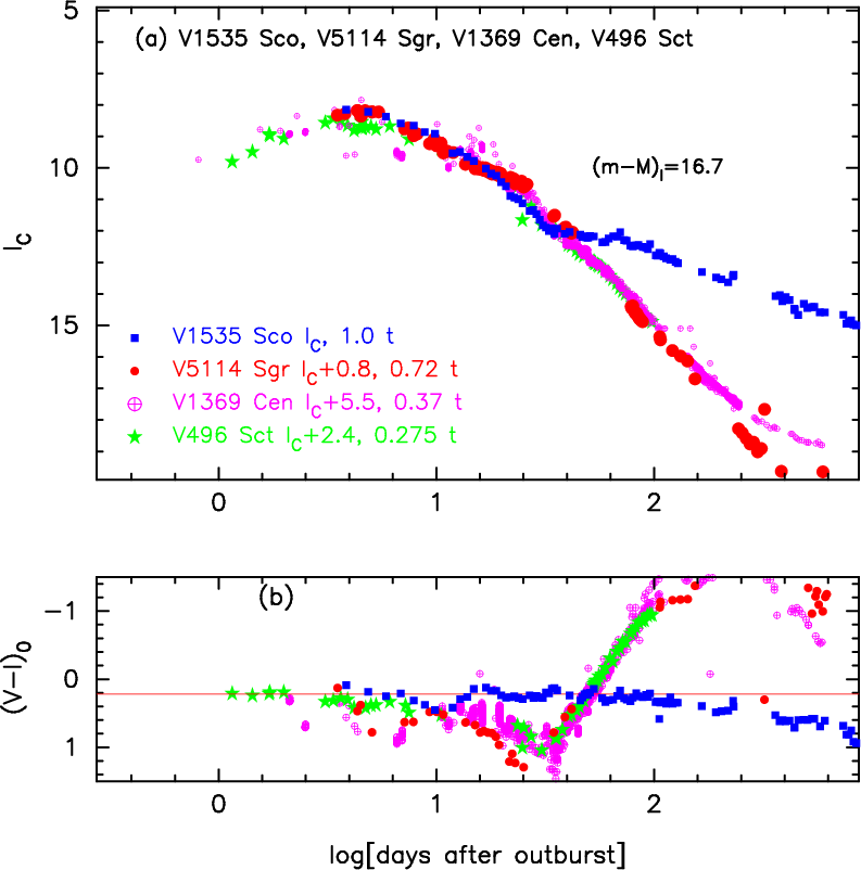
The U​B​VUBV Color Evolution of Classical Novae. IV. Time-Stretched (U−B)0(U-B)_{0}-(MB−2.5​log⁡fs)(M_{B}-2.5\log f_{\rm s}) and (V−I)0(V-I)_{0}-(MI−2.5​log⁡fs)(M_{I}-2.5\log f_{\rm s}) Color-Magnitude Diagrams of Novae in Outburst

Izumi Hachisu OrcID: 0000-0002-0884-7404 Affiliation: Department of Earth Science and Astronomy, College of Arts and Sciences, The University of Tokyo, 3-8-1 Komaba, Meguro-ku, Tokyo 153-8902, Japan Email: izumi.hachisu@outlook.jp Corresponding author: Izumi Hachisu    Mariko Kato OrcID: 0000-0002-8522-8033 Affiliation: Department of Astronomy, Keio University, Hiyoshi, Kouhoku-ku, Yokohama 223-8521, Japan
Abstract

Light curves and color evolutions of two classical novae can be largely overlapped if we properly squeeze or stretch the timescale of a target nova against that of a template nova by t′=t/fst^{\prime}=t/f_{\rm s}. Then the brightness of the target nova is related to the brightness of the template nova by (M⁡[t])template=(M⁡[t/fs]−2.5​log⁡fs)target(M[t])_{\rm template}=(M[t/f_{\rm s}]-2.5\log f_{\rm s})_{\rm target}, where M⁡[t]M[t] is the absolute magnitude and a function of time tt, and fsf_{\rm s} is the ratio of timescales between the target and template novae. In the previous papers of this series, we show that many novae broadly overlap in the time-stretched (B−V)0(B-V)_{0}-(MV−2.5​log⁡fs)(M_{V}-2.5\log f_{\rm s}) color-magnitude diagram. In the present paper, we propose two other (U−B)0(U-B)_{0}-(MB−2.5​log⁡fs)(M_{B}-2.5\log f_{\rm s}) and (V−I)0(V-I)_{0}-(MI−2.5​log⁡fs)(M_{I}-2.5\log f_{\rm s}) diagrams, and show that their tracks overlap for 16 novae and for 52 novae, respectively. Here, (U−B)0(U-B)_{0}, (B−V)0(B-V)_{0}, and (V−I)0(V-I)_{0} are the intrinsic U−BU-B, B−VB-V, and V−IV-I colors and not changed by the time-stretch, and MBM_{B}, MVM_{V}, and MIM_{I} are the absolute BB, VV, and II magnitudes. Using these properties, we considerably refine the previous estimates of their distance and reddening. The obtained distances are in reasonable agreement with those of Gaia Data Release 2 catalogue.

Keywords: 
novae, cataclysmic variables — stars: individual (V2659 Cyg, V496 Sct, V5114 Sgr, V959 Mon) — stars: winds

I Introduction

A nova is a thermonuclear runaway event on a mass-accreting white dwarf (WD). Hydrogen burning explosion releases nuclear energy that results in an expansion of a hydrogen-rich envelope to a giant size. Strong winds are accelerated deep inside the photosphere owing to the iron peak of the opacity. They are called optically thick winds (Kato & Hachisu 1994, e.g.,). The wind mass-loss rate increases as the photosphere is expanding. The nova brightness also increases, if we assume that free-free emission dominates the spectra of novae (Ennis et al. 1977; Gallagher & Ney 1976; Krautter et al. 1984; Naik et al. 2009, e.g.,), because the brightness of free-free emission depends mainly on the wind mass-loss rate (Hachisu & Kato 2006; Hachisu & Kato 2015, e.g.,). The nova brightness begins to decline after the maximum wind mass-loss rate is attained (Hachisu & Kato 2017, e.g.,). After a significant part of the hydrogen-rich envelope is blown in the wind, the winds stop. The nova enters the supersoft X-ray source (SSS) phase. The hydrogen nuclear burning extinguishes and the nova ends (Kato et al. 2014; Kato & Hachisu 2020, e.g.,).

Kato & Hachisu 1994 calculated optically thick winds to follow nova evolutions in the decay phase and obtained the photospheric radius RphR_{\rm ph}, photospheric temperature TphT_{\rm ph}, photospheric luminosity LphL_{\rm ph}, photospheric velocity vphv_{\rm ph}, and wind mass-loss rate M˙wind\dot{M}_{\rm wind}, for hydrogen-rich envelopes of various WD masses and chemical compositions. Using these physical quantities, Hachisu & Kato 2006 calculated many free-free emission model light curves with Fν∝M˙wind2/(vph2​Rph)F_{\nu}\propto\dot{M}_{\rm wind}^{2}/(v_{\rm ph}^{2}R_{\rm ph}), where FνF_{\nu} is the flux at the frequency ν\nu. The free-free flux is almost independent of the frequency, so the light curve shapes are almost the same among broad band light curves such as MBM_{B}, MVM_{V}, and MIM_{I}, where MBM_{B}, MVM_{V}, and MIM_{I} are the absolute magnitudes for BB, VV, and II bands, respectively.

The theoretical light curves also show a homologous shape independent of the WD mass and chemical composition. They called this property of nova model light curves “the universal decline law.” These properties, i.e., homologous and frequency independent shapes of light curves, are extremely useful for analysis of novae. For the light curve shapes, Hachisu & Kato 2010 found that the time-stretched absolute VV brightnesses of the model light curves, MV−2.5​log⁡fsM_{V}-2.5\log f_{\rm s}, overlap each other in the (t/fs)(t/f_{\rm s})-(MV−2.5​log⁡fs)(M_{V}-2.5\log f_{\rm s}) light curve (Hachisu & Kato 2018b, see, e.g., Figures 48 and 49 of). They explained this property in more detail in Appendix B of Hachisu & Kato 2019b, that is, if the VV light curve of a template nova overlaps with that of a target nova by squeezing its timescale as t′=t/fst^{\prime}=t/f_{\rm s}, we have the relation

(MV​[t])template\displaystyle\left(M_{V}[t]\right)_{\rm template} =\displaystyle= (MV′​[t′])target\displaystyle\left(M^{\prime}_{V}[t^{\prime}]\right)_{\rm target} (1)
=\displaystyle= (MV​[t/fs]−2.5​log⁡fs)target,\displaystyle\left(M_{V}[t/f_{\rm s}]-2.5\log f_{\rm s}\right)_{\rm target}, (2)

where MV​[t]M_{V}[t] is the original absolute VV brightness and MV′​[t′]M^{\prime}_{V}[t^{\prime}] is the time-stretched brightness after time-stretch of t′=t/fst^{\prime}=t/f_{\rm s} (Hachisu et al. 2020, see also ).

The similarity among different broad band light curves such as MUM_{U}, MBM_{B}, MVM_{V}, and MIM_{I} strongly suggests a common path (or track) of nova outburst evolutions in the color-magnitude diagram. In the first paper of this series (Hachisu & Kato 2014, hereafter Paper I), they found that many nova outbursts follow a part of the common path in the (B−V)0(B-V)_{0}-(U−B)0(U-B)_{0} color-color diagram. Here, (B−V)0(B-V)_{0} and (U−B)0(U-B)_{0} are the intrinsic B−VB-V and U−BU-B colors, respectively. They called this common path “the nova-giant sequence.” In the second paper of this series (Hachisu & Kato 2016b, hereafter Paper II), they studied 40 novae in outburst in the (B−V)0(B-V)_{0}-MVM_{V} color-magnitude diagram. They proposed six different types of tracks in the (B−V)0(B-V)_{0}-MVM_{V} diagram (Hachisu & Kato 2016b, see Figure 12 of).

In the third paper of this series (Hachisu & Kato 2019a, hereafter Paper III), they revised Hachisu & Kato’s (2016b) naive method and studied 20 novae in outburst in the time-stretched color-magnitude diagram, (B−V)0(B-V)_{0}-(MV−2.5​log⁡fs)(M_{V}-2.5\log f_{\rm s}). They found that many novae follow one of the two template paths in the (B−V)0(B-V)_{0}-(MV−2.5​log⁡fs)(M_{V}-2.5\log f_{\rm s}) diagram. Hachisu & Kato 2019b further applied this new method to 32 recent novae. This paper, the fourth of this series, extends our time-stretched color-magnitude diagram method to U​B​V​IUBVI bands, i.e., the (U−B)0(U-B)_{0}-(MB−2.5​log⁡fs)(M_{B}-2.5\log f_{\rm s}) and (V−I)0(V-I)_{0}-(MI−2.5​log⁡fs)(M_{I}-2.5\log f_{\rm s}) diagrams. We try to find similar common tracks even in these time-stretched color-magnitude diagrams. Moreover, we show that, newly including the UU, BB, and II data in our analysis, we can determine the color excess E⁡(B−V)E(B-V), distance moduli (m−M)U(m-M)_{U}, (m−M)B(m-M)_{B}, (m−M)V(m-M)_{V}, (m−M)I(m-M)_{I}, and timescaling factor fsf_{\rm s}, more precisely.

Our paper is organized as follows. First we propose the time-stretched (U−B)0(U-B)_{0}-(MB−2.5​log⁡fs)(M_{B}-2.5\log f_{\rm s}) diagrams for 16 novae in Section II and then the time-stretched (V−I)0(V-I)_{0}-(MI−2.5​log⁡fs)(M_{I}-2.5\log f_{\rm s}) diagrams for 52 novae in Sections III, IV, V, and VI. Our conclusions are given in Section VII. Appendix A introduces our time-stretching method to obtain the distances and extinctions of each nova. Here, we reanalyzed four novae newly including II magnitude data. Other 44 novae, which are once analyzed in our previous papers, are reanalyzed in Appendix B.

It should be noted that our theoretical model light curves are calculated from free-free emission and do not include the effects of bound-bound and free-bound emissions. Therefore, if such effects contribute significantly to the spectra of novae, our model light curves deviate from the observation. Such an example is the VV band light curve in the nebular phase, in which strong emission lines such as [O III] contribute to the VV band. We already discussed such deviations in our previous papers (Hachisu & Kato 2006; Hachisu & Kato 2010; Hachisu & Kato 2014; Hachisu & Kato 2015; Hachisu & Kato 2016a; Hachisu & Kato 2018b; Hachisu & Kato 2019a; Hachisu & Kato 2019b, e.g.). Our model light curves reproduce reasonably well such nova VV light curves except for the nebular phase as already shown in our previous papers and also in Appendixes A and B of the present paper. As concerns to the free-bound emission in the continuum, this can affect mainly the UU magnitude due to the Balmer jump in emission (Skopal 2019, see, e.g., Figure 3 of).

To formulate the time-stretched color-magnitude diagram, we use the nature of nova light curves described by Equation (2), that is, time-stretched nova light curves overlap each other with the time-scaling factor of fsf_{\rm s}. This nature can be derived from the universal decline law of novae. The universal decline law was derived from the nova model light curves based on optically thick wind and free-free emission. This relation has been calibrated on many novae (Hachisu & Kato 2016a; Hachisu & Kato 2016b; Hachisu & Kato 2018b; Hachisu & Kato 2019a; Hachisu & Kato 2019b, e.g.,). Once we accept Equation (2), we do not use the universal decline law or nova model light curves, but directly compare template novae with target novae. In this circumstance, it is obvious that each template or target nova includes all effects that are significant in the spectra.

Refer to caption
Figure 1: Time-stretched (U−B)0(U-B)_{0}-(MB−2.5​log⁡fs)(M_{B}-2.5\log f_{\rm s}) color-magnitude diagrams for (a) LV Vul, (b) V1500 Cyg, (c) V1668 Cyg, and (d) V1974 Cyg. We obtain template tracks for LV Vul (thick orange line), V1500 Cyg (thick green line), V1668 Cyg (thick cyan-blue line), and V1974 Cyg (thick magenta line), all from the observed data. The large unfilled red squares denote the positions at the start of nebular phase. The large unfilled blue square indicates the start of dust shell formation. In panel (d), the black arrow labeled “SSS on” indicates the start of the supersoft X-ray source (SSS) phase. Each smaller symbol shows the source of data. See the text for more details.
Refer to caption
Figure 2: Same as Figure 1, but for (a) V446 Her, (b) V533 Her, (c) FH Ser, and (d) IV Cep. The thick light-green lines denote the template track of V446 Her. In panel (c), we add the template track of V1974 Cyg (thick cyan line). In panel (d), the thick cyan-blue line denotes the template track of IV Cep.

II Time-Stretched (U−B)0(U-B)_{0}-(MB−2.5​log⁡fs)(M_{B}-2.5\log f_{\rm s}) Color-Magnitude Diagram

We examine (U−B)0(U-B)_{0}-(MB−2.5​log⁡fs)(M_{B}-2.5\log f_{\rm s}) diagram in the first time of this series of papers. In recent CCD photometric observations, UU band filters are not frequently used. We adopt 16 novae having rich UU data. Most of them are already examined in our previous papers (Hachisu & Kato 2016b; Hachisu & Kato 2018b; Hachisu & Kato 2019a; Hachisu & Kato 2019b), but without information of the (U−B)0(U-B)_{0}-(MB−2.5​log⁡fs)(M_{B}-2.5\log f_{\rm s}) diagram. Their timescaling factors, distances, color excesses, and absolute VV magnitudes are well determined. In what follows, we obtain (U−B)0(U-B)_{0}-(MB−2.5​log⁡fs)(M_{B}-2.5\log f_{\rm s}) diagrams of 16 novae and plot their color-magnitude diagram in Figures 1-5. Among them, LV Vul, V1500 Cyg, V1668 Cyg, V1974 Cyg, FH Ser, and PU Vul are the six template novae proposed by Hachisu & Kato 2016b.

We obtain the intrinsic colors via

(B−V)0=(B−V)−E⁡(B−V),(B-V)_{0}=(B-V)-E(B-V), (3)

and

(U−B)0=(U−B)−0.64​E​(B−V),(U-B)_{0}=(U-B)-0.64E(B-V), (4)

where the factor of 0.640.64 is taken from Rieke & Lebofsky 1985. The distance modulus in BB band, (m−M)B(m-M)_{B}, is usually taken from Hachisu & Kato 2019a; Hachisu & Kato 2019b, Appendix A, or Appendix B. Then, its time-stretched value is calculated from

(m−M′)B≡(m−(M−2.5​log⁡fs))B.(m-M^{\prime})_{B}\equiv(m-(M-2.5\log f_{\rm s}))_{B}. (5)

We adopt the relations between the distance moduli in VV, BB, and UU, distance, and color excess to a nova, i.e.,

(m−M)V=3.1​E​(B−V)+5​log⁡(d/10​pc),\displaystyle(m-M)_{V}=3.1E(B-V)+5\log(d/10~{\rm pc}), (6)
(m−M)B=4.1​E​(B−V)+5​log⁡(d/10​pc),\displaystyle(m-M)_{B}=4.1E(B-V)+5\log(d/10~{\rm pc}), (7)

and

(m−M)U=4.75​E​(B−V)+5​log⁡(d/10​pc),\displaystyle(m-M)_{U}=4.75E(B-V)+5\log(d/10~{\rm pc}), (8)

where the factor RV=AV/E⁡(B−V)=3.1R_{V}=A_{V}/E(B-V)=3.1, AB/E⁡(B−V)=4.1A_{B}/E(B-V)=4.1, and AU/E⁡(B−V)=4.75A_{U}/E(B-V)=4.75 are the ratios of total to selective extinctions (Rieke & Lebofsky 1985).

II.1 LV Vul 1968#1

LV Vul is a typical classical nova and its various properties were discussed in Hachisu & Kato 2014; Hachisu & Kato 2016b. The peak VV brightness is MV=−7.15M_{V}=-7.15. Hachisu & Kato 2019a; Hachisu & Kato 2019b adopted LV Vul as a template nova, against which they measured the timescaling factor fsf_{\rm s} of a target nova. Based on the time-stretching method (Hachisu & Kato 2010), Hachisu & Kato 2019a obtained E⁡(B−V)=0.60E(B-V)=0.60, (m−M)V=11.85(m-M)_{V}=11.85, d=1.0d=1.0 kpc, and log⁡fs=0.0\log f_{\rm s}=0.0 for LV Vul. Recent distance determination based on Gaia Data Release2 (Gaia DR2) trigonometric parallax shows similar values of d=0.91±0.12d=0.91\pm 0.12 kpc (Tappert et al. 2020). These values are summarized in Table 1 of Hachisu & Kato 2019b. We have (m−M)B=12.45(m-M)_{B}=12.45 and (m−M′)B=12.45+0.0=12.45(m-M^{\prime})_{B}=12.45+0.0=12.45 from Hachisu & Kato 2019a. We plot the (U−B)0(U-B)_{0}-(MB−2.5​log⁡fs)(M_{B}-2.5\log f_{\rm s}) diagram in Figure 1(a). Here, we adopt the U​B​VUBV data from Abuladze 1969, Dorschner et al. 1969, and Fernie 1969. We have the peak BB brightness of MB′≡MB−2.5​log⁡fs=−7.0−0.0=−7.0M^{\prime}_{B}\equiv M_{B}-2.5\log f_{\rm s}=-7.0-0.0=-7.0. In Figure 1(a), the text “(m-M’)B=12.45(+0.0)” means that (m−M′)B=12.45(m-M^{\prime})_{B}=12.45 and (m−M)B=12.45+0.0=12.45(m-M)_{B}=12.45+0.0=12.45.

We define the template track of LV Vul by the thick solid orange line. In the rising phase of BB magnitude, the (U−B)0(U-B)_{0} color goes toward the red (right) until (U−B)0∼−0.2(U-B)_{0}\sim-0.2 and then turns back to the blue (left). It horizontally moves blueward near the peak and then goes down. After the start of the nebular phase (large unfilled red square), it turns to the red. This is because strong emission lines contribute much more to the BB band than to the UU band in the nebular phase.

II.2 V1500 Cyg 1975

V1500 Cyg is also a well-examined nova in this series of papers. Hachisu & Kato 2019a proposed V1500 Cyg as another template nova. We have reanalyzed this nova including the (V−I)0(V-I)_{0} color curves in Appendix B.1 and revised the timescaling factor from log⁡fs=−0.22\log f_{\rm s}=-0.22 (Hachisu & Kato 2019a) to the present log⁡fs=−0.28\log f_{\rm s}=-0.28 to overlap the (V−I)0(V-I)_{0} color curves. Correspondingly, the distance modulus in VV band, (m−M)V(m-M)_{V}, is slightly changed from the old value of (m−M)V=12.3(m-M)_{V}=12.3 (Hachisu & Kato 2019a) to a new value of (m−M)V=12.15(m-M)_{V}=12.15. We finally obtain E⁡(B−V)=0.45E(B-V)=0.45 and d=1.4d=1.4 kpc (see Figure 54(b) in Appendix B). Recent distance determination based on Gaia DR2 trigonometric parallaxes shows a similar value of d=1.29±0.31d=1.29\pm 0.31 kpc (della Valle & Izzo 2020). These new parameters are listed in Tables 1 and 2. Then, we plot the (U−B)0(U-B)_{0}-(MB−2.5​log⁡fs)(M_{B}-2.5\log f_{\rm s}) diagram in Figure 1(b). Here, we adopt the U​B​VUBV data from Kiselev & Narizhnaia 1977, Lindgren 1979, Pfau 1976, and Williamon 1977.

V1500 Cyg is a super-bright nova and its peak magnitudes are MV=−10.3M_{V}=-10.3 and MB=−10.1M_{B}=-10.1. Here, we adopt the distance modulus in BB band, (m−M)B=12.6(m-M)_{B}=12.6 from Appendix B.1. We have (m−M′)B=12.6−0.7=11.9(m-M^{\prime})_{B}=12.6-0.7=11.9. In Figure 1(b), the time-stretched peak BB brightness is MB′≡MB−2.5​log⁡fs=−10.1+0.7=−9.4M^{\prime}_{B}\equiv M_{B}-2.5\log f_{\rm s}=-10.1+0.7=-9.4.

We define the template track of V1500 Cyg by the thick solid green line. It moves redward until (U−B)0∼−0.35(U-B)_{0}\sim-0.35 before the peak and comes back toward the blue. After the peak it goes down almost straight. The track overlaps with that of LV Vul between MB′=MB−2.5​log⁡fs∼−6M^{\prime}_{B}=M_{B}-2.5\log f_{\rm s}\sim-6 and −4-4. After the nebular phase starts, the track departs from LV Vul. This is because strong [Ne III] and [Ne V] lines contribute to the UU band in the nebular phase. The two tracks of V1500 Cyg and LV Vul are closely located only in their middle phases, because their peak brightnesses are very different in the early phase and strong emission line contributions are different in the later nebular phase.

II.3 V1668 Cyg 1978

V1668 Cyg is a well-observed nova and its peak VV brightness is MV=−8.6M_{V}=-8.6. Hachisu & Kato 2019a obtained E⁡(B−V)=0.30E(B-V)=0.30, (m−M)V=14.6(m-M)_{V}=14.6, d=5.4d=5.4 kpc, and log⁡fs=0.0\log f_{\rm s}=0.0. We plot the (U−B)0(U-B)_{0}-(MB−2.5​log⁡fs)(M_{B}-2.5\log f_{\rm s}) diagram in Figure 1(c). Here, the U​B​VUBV data are taken from Duerbeck et al. 1980 and Mallama & Skillman 1979.

The distance modulus in BB band, (m−M)B=14.9(m-M)_{B}=14.9, is taken from Hachisu & Kato 2019a. Then, we have (m−M′)B=14.9+0.0=14.9(m-M^{\prime})_{B}=14.9+0.0=14.9. The time-stretched peak BB brightness is MB′=MB−2.5​log⁡fs=−8.3+0.0=−8.3M^{\prime}_{B}=M_{B}-2.5\log f_{\rm s}=-8.3+0.0=-8.3 as shown in Figure 1(c). We define the template track of V1668 Cyg by the thick cyan-blue line. It moves blueward near the peak, goes down almost straight, and then turns to the red after the start of nebular phase. The shape of the track is very similar to that of LV Vul except for the early phase because of the brighter peak by −1.3-1.3 mag than that of LV Vul.

II.4 V1974 Cyg 1992

V1974 Cyg is a well-observed neon nova and its peak VV brightness is MV=−8.0M_{V}=-8.0. Hachisu & Kato 2019a obtained E⁡(B−V)=0.30E(B-V)=0.30, (m−M)V=12.2(m-M)_{V}=12.2, d=1.8d=1.8 kpc, and log⁡fs=+0.03\log f_{\rm s}=+0.03 for V1974 Cyg. Recent distance determination based on Gaia DR2 shows a similar value of d=1631−131+261d=1631^{+261}_{-131} pc (Schaefer 2018). We plot the (U−B)0(U-B)_{0}-(MB−2.5​log⁡fs)(M_{B}-2.5\log f_{\rm s}) diagram in Figure 1(d). Here, the U​B​VUBV data are taken from Chochol et al. 1993.

The distance modulus in BB band, (m−M)B=12.5(m-M)_{B}=12.5, is taken from Hachisu & Kato 2019a. Then, we have (m−M′)B=12.5+0.075=12.6(m-M^{\prime})_{B}=12.5+0.075=12.6. The time-stretched peak BB brightness is MB′=MB−2.5​log⁡fs=−7.3−0.075=−7.4M^{\prime}_{B}=M_{B}-2.5\log f_{\rm s}=-7.3-0.075=-7.4 as shown in Figure 1(d). We define the template track of V1974 Cyg by the thick solid magenta line. It moves blueward near the peak, goes down almost straight, and then splits into two branches after the start of nebular phase. This is because there are small differences between the BB filters at their blue edges and strong emission lines such as [Ne III] contribute differently to their BB magnitudes. The shape of the right track is similar to that of LV Vul or V1668 Cyg except for the peak BB brightness, while the left branch moves greatly to the blue due to the strong contributions of [Ne III] and [Ne V] emission lines to the UU band than the contribution of [Ne III] emission to the BB band.

The difference in the inclinations of tracks after the start of SSS phase in Figure 1(d) could partly originate from the following effects: Just prior to and during the SSS phase, a rise of the WD temperature increases also electron temperature of the ionized ejecta, which makes the nebular continuum steeper, and thus bluer indices. Following the SSS phase, the situation can be opposite, although the effect of emission lines is probably dominant (see, Figures 38, 39, 43, 46, 49, etc.).

II.5 V446 Her 1960

Hachisu & Kato 2019a obtained E⁡(B−V)=0.40E(B-V)=0.40, (m−M)V=11.95(m-M)_{V}=11.95, d=1.38d=1.38 kpc, and log⁡fs=0.0\log f_{\rm s}=0.0 for V446 Her. Recent distance determination based on Gaia DR2 shows similar values of d=1361−100+185d=1361^{+185}_{-100} pc (Schaefer 2018) and d=1308±130d=1308\pm 130 pc (Selvelli & Gilmozzi 2019). We plot the (U−B)0(U-B)_{0}-(MB−2.5​log⁡fs)(M_{B}-2.5\log f_{\rm s}) diagram in Figure 2(a). Here, we adopt the U​B​VUBV data from IAU Circular No. 7176, 7179, 7196, 7209, 7216, 7226, 7232, 7238, 7277, and Ross 1960 and Bronkalla & Notni 1961. From Equation (7), we have (m−M)B=12.35(m-M)_{B}=12.35. Then, we have (m−M′)B=12.35+0.0=12.35(m-M^{\prime})_{B}=12.35+0.0=12.35 as shown in Figure 2(a).

We define the template track of V446 Her by the thick solid light-green line. The peak BB brightness was probably missed. The track goes down almost straight and splits into two branches near MB′=MB−2.5​log⁡fs≈−6M^{\prime}_{B}=M_{B}-2.5\log f_{\rm s}\approx-6. The left branch (light-green) follows the data of Ross 1960 and Bronkalla & Notni 1961 while the right branch (green) follows the data of IAU Circular. This split is caused by small differences at blue edges of the BB filters together with strong emission lines such as [Ne III] that contribute differently to their BB magnitudes. We define the track of V446 Her by the left branch (light-green line). Comparing with V1500 Cyg (green line), the middle part of the track is Δ⁡(U−B)∼0.3\Delta(U-B)\sim 0.3 mag bluer whereas the early and late parts overlap with the V1500 Cyg track.

II.6 V533 Her 1963

Hachisu & Kato 2019a obtained E⁡(B−V)=0.038E(B-V)=0.038, (m−M)V=10.65(m-M)_{V}=10.65, d=1.28d=1.28 kpc, and log⁡fs=+0.08\log f_{\rm s}=+0.08 for V533 Her. Recent distance determination based on Gaia DR2 shows similar values of d=1202−42+51d=1202^{+51}_{-42} pc (Schaefer 2018) and d=1165±44d=1165\pm 44 pc (Selvelli & Gilmozzi 2019). From Equation (7), we have (m−M)B=10.7(m-M)_{B}=10.7 and (m−M′)B=10.7+0.2=10.9(m-M^{\prime})_{B}=10.7+0.2=10.9. We plot the (U−B)0(U-B)_{0}-(MB−2.5​log⁡fs)(M_{B}-2.5\log f_{\rm s}) diagram in Figure 2(b). The U​B​VUBV data are taken from van Genderen 1963, Chincarini 1964, and Shen et al. 1964.

The peak BB brightness was missed. The data points are so scattered among the three observers, but broadly follow the LV Vul track (orange line).

Refer to captionRefer to caption

Figure 3: Time-stretched (B−V)0(B-V)_{0}-(MV−2.5​log⁡fs)(M_{V}-2.5\log f_{\rm s}) color-magnitude diagram of FH Ser (a) and various distance-reddening relations toward FH Ser (b). In panel (a), the solid black line represents the template track of FH Ser while the thick solid green, orange, and magenta lines denote the template tracks of V1500 Cyg, LV Vul, and V1974 Cyg, respectively. The points A, B, C, and D on the black line correspond to the same points in Figure 2 of Hachisu & Kato 2014. In panel (b), the three thin solid lines of green, cyan, and blue denote the distance-reddening relations given by (m−M)U=12.9(m-M)_{U}=12.9, (m−M)B=12.5(m-M)_{B}=12.5, and (m−M)V=11.9(m-M)_{V}=11.9, respectively. We add four distance-reddening relations (thick cyan-blue lines) of Chen et al. 2019, which correspond to four nearby directions toward FH Ser, i.e., the galactic coordinates of (ℓ,b)=(32​.∘​85,+5​.∘​75)(\ell,b)=(32\fdg 85,+5\fdg 75), (32​.∘​85,+5​.∘​85)(32\fdg 85,+5\fdg 85), (32​.∘​95,+5​.∘​85)(32\fdg 95,+5\fdg 85), and (32​.∘​95,+5​.∘​75)(32\fdg 95,+5\fdg 75). We also add the distance-reddening relation (thick solid yellow line) toward FH Ser given by Green et al. 2019. Other symbols and lines are the same as those in Figure 41.
Refer to caption
Figure 4: Same as Figure 1, but for (a) PW Vul, (b) V1419 Aql, (c) V382 Vel, and (d) V5114 Sgr. In panel (b), we add the track of FH Ser (filled cyan stars). In panels (c) and (d), the vertical solid red lines show the intrinsic U−BU-B color of optically-thick free-free emission, that is, (U−B)0=−0.97(U-B)_{0}=-0.97 (Hachisu & Kato 2014). In panel (c), we add the tracks of V1974 Cyg (thick solid cyan lines) and V1668 Cyg (cyan-blue lines). In panel (d), we add the track of IV Cep (cyan-blue line).
Refer to caption
Figure 5: Same as Figure 1, but for (a) U Sco, (b) T Pyx, (c) V2659 Cyg, and (d) PU Vul. In panel (c), we add the template track of IV Cep (cyan-blue line). In panel (d), the thick solid magenta line denotes the template track of V1974 Cyg.
Refer to caption
Figure 6: Color-color diagrams of (a) PW Vul, (b) V382 Vel, (c) V5114 Sgr, and (d) U Sco. The thick solid green lines denote the track of nova-giant sequence defined by Hachisu & Kato 2014. We also show the three other sequences, i.e., blackbody, main-sequence, and supergiant sequences (Hachisu & Kato 2014, see, e.g.,). The unfilled black diamond denotes the position of optically thick free-free emission (Wright & Barlow 1975, Fν∝ν2/3F_{\nu}\propto\nu^{2/3}, ), whose colors are (B−V)0=−0.03(B-V)_{0}=-0.03 and (U−B)0=−0.97(U-B)_{0}=-0.97 (Hachisu & Kato 2014). See the text for the sources of observational data.
Refer to caption
Figure 7: Same as Figure 6, but for (a) T Pyx, (b) V2659 Cyg, (c) Pre-maximum phase of PU Vul, and (d) Post-maximum phase of PU Vul. In panels (c) and (d), the attached numbers (1-5) to the unfilled triangles denote the epochs of light curve of PU Vul in Figure 15 of Hachisu & Kato 2014, and the attached alphabets (A-D) to the filled purple circles represent the epochs of light curve of FH Ser in Figure 2 of Hachisu & Kato 2014 (see also Figure 3(a)). The solid purple line corresponds to the track of FH Ser, which is designated the nova-giant sequence by Hachisu & Kato 2014. The points labeled “F” (open black diamond) and “O” (open black square) are the positions of optically-thick and optically-thin free-free emission, respectively.

II.7 FH Ser 1970

Hachisu & Kato 2016b obtained E⁡(B−V)=0.60E(B-V)=0.60, (m−M)V=11.7(m-M)_{V}=11.7, and d=0.93d=0.93 kpc. Recent distance determination based on Gaia DR2 shows a similar value of d=1060−68+112d=1060^{+112}_{-68} pc (Schaefer 2018). We have determined the timescaling factor of log⁡fs=+0.40\log f_{\rm s}=+0.40 as well as (m−M)U=12.9(m-M)_{U}=12.9, (m−M)B=12.5(m-M)_{B}=12.5, (m−M)V=11.9(m-M)_{V}=11.9, and d=1.0d=1.0 kpc from Figures 106, 163, and 166(a) in Appendix B. These new parameters are listed in Tables 1 and 2. Then, we have (m−M′)B=12.5+1.0=13.5(m-M^{\prime})_{B}=12.5+1.0=13.5. The time-stretched peak BB brightness is MB′=MB−2.5​log⁡fs=−7.0−1.0=−8.0M^{\prime}_{B}=M_{B}-2.5\log f_{\rm s}=-7.0-1.0=-8.0. We plot the (U−B)0(U-B)_{0}-(MB−2.5​log⁡fs)(M_{B}-2.5\log f_{\rm s}) diagram in Figure 2(c). The U​B​VUBV data are taken from Borra & Andersen 1970, Osawa 1970, and Burkhead et al. 1971. The track almost horizontally moves blueward near the peak. Then, it almost vertically goes down up to the formation of an optically-thick dust shell, which clouds the following evolution. The track is located close to the track of V1974 Cyg (cyan line) in the early phase.

We also plot the (B−V)0(B-V)_{0}-(MV−2.5​log⁡fs)(M_{V}-2.5\log f_{\rm s}) diagram in Figure 3(a). The track of FH Ser is located close to the track of V1974 Cyg (magenta line) until the dust blackout started. The solid black line represents the template track of FH Ser and four points, A, B, C, and D are the same points as those in Figure 2 of Hachisu & Kato 2014. We obtain (m−M)U=12.9(m-M)_{U}=12.9, (m−M)B=12.5(m-M)_{B}=12.5, and (m−M)V=11.9(m-M)_{V}=11.9 from our time-stretching method in Figures 166(a), 163, and 106, respectively. We plot their distance-reddening relations, i.e., Equations (8), (7), and (6), respectively, in Figure 3(b). These three lines broadly cross at d=1.0d=1.0 kpc and E⁡(B−V)=0.60E(B-V)=0.60. This crossing point is consistent with the distance-reddening relations given by Green et al. 2018, Green et al. 2019, Özdörmez et al. 2018, and Marshall et al. 2006.

II.8 IV Cep 1971

Hachisu & Kato 2018a obtained E⁡(B−V)=0.65E(B-V)=0.65, (m−M)V=14.5(m-M)_{V}=14.5, d=3.1d=3.1 kpc, and log⁡fs=0.0\log f_{\rm s}=0.0 for IV Cep. From Equation (7), we have (m−M)B=15.15(m-M)_{B}=15.15 and then have (m−M′)B=15.15+0.0=15.15(m-M^{\prime})_{B}=15.15+0.0=15.15. We plot the (U−B)0(U-B)_{0}-(MB−2.5​log⁡fs)(M_{B}-2.5\log f_{\rm s}) diagram in Figure 2(d). The U​B​VUBV data are taken from MacConnell & Thomas 1972 and Kohoutek & Klawitter 1973.

The peak in the BB band was missed. The track goes down almost straight and then turns to the right (redward) just after the start of nebular phase. It almost follows the track of LV Vul (orange line).

II.9 PW Vul 1984#1

Hachisu & Kato 2019a obtained E⁡(B−V)=0.57E(B-V)=0.57, (m−M)V=13.0(m-M)_{V}=13.0, d=1.8d=1.8 kpc, and log⁡fs=+0.35\log f_{\rm s}=+0.35 for PW Vul. Recent distance determination based on Gaia DR2 shows a slightly larger value of d=2420−277+1337d=2420^{+1337}_{-277} pc (Schaefer 2018). We have reanalyzed the U​B​V​IUBVI data of PW Vul based on the time-stretching method in Appendix B.2, including the (t/fs)(t/f_{\rm s})-(MI−2.5​log⁡fs)(M_{I}-2.5\log f_{\rm s}) light curve and (t/fs)(t/f_{\rm s})-(V−I)0(V-I)_{0} color curve fitting. We have obtained a new parameter set of E⁡(B−V)=0.40E(B-V)=0.40, (m−M)U=13.88(m-M)_{U}=13.88, (m−M)B=13.6(m-M)_{B}=13.6, (m−M)V=13.2(m-M)_{V}=13.2, (m−M)I=12.55(m-M)_{I}=12.55, d=2.46d=2.46 kpc, and log⁡fs=+0.30\log f_{\rm s}=+0.30. These new parameters are listed in Tables 1 and 2. The new distance estimate is consistent with the distance of Gaia DR2. The main difference is the color excess. The new color excess of E⁡(B−V)=0.40E(B-V)=0.40 is consistent with several distance-reddening relations as shown in Figure 58(b) of Appendix B.2. We plot the (B−V)0(B-V)_{0}-(U−B)0(U-B)_{0} color-color diagram of PW Vul in Figure 6(a). The new track of PW Vul (filled red circles) is quite consistent with the template tracks of nova-giant sequence (green lines) defined by Hachisu & Kato 2014.

In the (B−V)0(B-V)_{0}-(U−B)0(U-B)_{0} diagram, we denote the position of optically-thick free-free emission (unfilled black diamond). This position is accidentally coincident with the cross of blackbody sequence (black line) and nova-giant sequence (green line). It should be noted that the color indices (U−B)0=−0.97(U-B)_{0}=-0.97, (B−V)0=−0.03(B-V)_{0}=-0.03, and (V−I)0=+0.22(V-I)_{0}=+0.22 of free-free emission are derived from the continuum flux of Fν∝ν2/3F_{\nu}\propto\nu^{2/3} for the radio and infrared domains. This approximation corresponds to h​ν≪k​Teh\nu\ll kT_{\rm e} and is, strictly speaking, not valid in the optical region. Here, hh, ν\nu, kk, and TeT_{\rm e} are the Planck constant, frequency, Boltzmann constant, and electron temperature (Hachisu & Kato 2014, see, e.g., Equation (7) of). In the optical region, these three color indices can be a result of different contributions from different sources of radiation to the continuum during some stages of the nova evolution. Usually, the optical continuum is given by superposition of the blackbody (or atmospheric model) and the nebular radiation (or free-free emission). Hachisu & Kato 2014 showed that the continuum flux Fν∝ν2/3F_{\nu}\propto\nu^{2/3} in the optical region of PW Vul is well reproduced with the summation of the blackbody and optically-thick free-free emissions at this epoch (see their Figure 9). In this sense, the color indices (U−B)0=−0.97(U-B)_{0}=-0.97, (B−V)0=−0.03(B-V)_{0}=-0.03, and (V−I)0=+0.22(V-I)_{0}=+0.22 need not to represent the pure optically-thick free-free emission in the optical region.

We have (m−M′)B=13.6+0.75=14.35(m-M^{\prime})_{B}=13.6+0.75=14.35. The time-stretched peak BB brightness is MB′=MB−2.5​log⁡fs=−6.64−0.75=−7.39M^{\prime}_{B}=M_{B}-2.5\log f_{\rm s}=-6.64-0.75=-7.39. We plot the (U−B)0(U-B)_{0}-(MB−2.5​log⁡fs)(M_{B}-2.5\log f_{\rm s}) diagram in Figure 4(a). Here, we adopt the U​B​VUBV data from Noskova et al. 1985, Kolotilov & Noskova 1986, and Robb & Scarfe 1995. The track almost follows the LV Vul template track (orange line) until the nebular phase started. The overlapping of PW Vul and LV Vul suggests a reasonable value of the color excess, E⁡(B−V)=0.40E(B-V)=0.40, because the horizontal shift of U−BU-B color determines the color excess of E⁡(U−B)=0.64​E​(B−V)E(U-B)=0.64E(B-V). The overlapping of PW Vul and LV Vul in the time-stretched color-magnitude diagram also supports the vertical fit with (m−M)B=13.6(m-M)_{B}=13.6, d=2.46d=2.46 kpc, and log⁡fs=+0.30\log f_{\rm s}=+0.30.

II.10 V1419 Aql 1993

Hachisu & Kato 2019a obtained E⁡(B−V)=0.52E(B-V)=0.52, (m−M)V=15.0(m-M)_{V}=15.0, d=4.7d=4.7 kpc, and log⁡fs=+0.15\log f_{\rm s}=+0.15 for V1419 Aql. The distance modulus in BB band, (m−M)B=15.5(m-M)_{B}=15.5, is calculated from Equation (7). Then, we have (m−M′)B=15.5+0.35=15.85(m-M^{\prime})_{B}=15.5+0.35=15.85. The time-stretched peak BB brightness is MB′=MB−2.5​log⁡fs=−7.1−0.35=−7.45M^{\prime}_{B}=M_{B}-2.5\log f_{\rm s}=-7.1-0.35=-7.45. We plot the (U−B)0(U-B)_{0}-(MB−2.5​log⁡fs)(M_{B}-2.5\log f_{\rm s}) diagram in Figure 4(b). Here, we adopt the U​B​VUBV data from IAU Circular No. 5794, 5802, 5807, 5829, and Munari et al. 1994. The track broadly follows LV Vul (orange line) until an optically thick dust shell formed. We also add the track of FH Ser (filled cyan stars). The V1419 Aql track almost overlaps with the track of FH Ser until the dust blackout of FH Ser.

II.11 V382 Vel 1999

Hachisu & Kato 2019a obtained E⁡(B−V)=0.25E(B-V)=0.25, (m−M)V=11.5(m-M)_{V}=11.5, d=1.4d=1.4 kpc, and log⁡fs=−0.29\log f_{\rm s}=-0.29 for V382 Vel. Recent distance determination based on Gaia DR2 shows a slightly larger value of d=1800−133+243d=1800^{+243}_{-133} pc (Schaefer 2018). We have reanalyzed the U​B​V​IUBVI data of V382 Vel based on the time-stretching method in Appendix B.4, including the (t/fs)(t/f_{\rm s})-(MI−2.5​log⁡fs)(M_{I}-2.5\log f_{\rm s}) light curve and (t/fs)(t/f_{\rm s})-(V−I)0(V-I)_{0} color curve fitting. We have obtained a new parameter set of E⁡(B−V)=0.12E(B-V)=0.12, (m−M)U=11.78(m-M)_{U}=11.78, (m−M)B=11.71(m-M)_{B}=11.71, (m−M)V=11.6(m-M)_{V}=11.6, (m−M)I=11.41(m-M)_{I}=11.41, d=1.76±0.2d=1.76\pm 0.2 kpc, and log⁡fs=−0.29\log f_{\rm s}=-0.29. These new parameters are listed in Tables 1 and 2. The new distance estimate is consistent with the distance of Gaia DR2. The main difference is the color excess. With the UU, BB, and II data being newly included in our analysis, we can determine the color excess more precisely. The new color excess of E⁡(B−V)=0.12E(B-V)=0.12 is consistent with the (B−V)0(B-V)_{0}-(U−B)0(U-B)_{0} color-color diagram of nova-giant sequence as shown in Figure 6(b) and the distance-reddening relation given by Chen et al. 2019 as shown in Figure 64(b) of Appendix B.4.

The distance modulus in BB band is (m−M)B=11.71(m-M)_{B}=11.71. Then, we have (m−M′)B=11.71−0.725=10.99(m-M^{\prime})_{B}=11.71-0.725=10.99. The peak BB brightness is MB′=MB−2.5​log⁡fs=−8.75+0.725=−8.0M^{\prime}_{B}=M_{B}-2.5\log f_{\rm s}=-8.75+0.725=-8.0. We plot the (U−B)0(U-B)_{0}-(MB−2.5​log⁡fs)(M_{B}-2.5\log f_{\rm s}) diagram in Figure 4(c). Here, we adopt the U​B​VUBV data from IAU Circular No. 7176, 7179, 7196, 7209, 7216, 7226, 7232, 7238, and 7277. The track almost follows V1668 Cyg (blue line) in the very early phase. Then, it follows the template track of V446 Her (light-green line). The overlapping of V382 Vel and V446 Her in the middle phase suggests that the color excess, E⁡(B−V)=0.12E(B-V)=0.12, is reasonable because the horizontal shift of U−BU-B color determines the color excess of E⁡(U−B)=0.64​E​(B−V)E(U-B)=0.64E(B-V).

The V382 Vel track also overlaps with that of the LV Vul template track in the (B−V)0(B-V)_{0}-(MV−2.5​log⁡fs)(M_{V}-2.5\log f_{\rm s}) diagram, that is, Figure 12(b). The V382 Vel track also overlaps with the V496 Sct/V959 Mon template tracks (orange lines) in the (V−I)0(V-I)_{0}-(MI−2.5​log⁡fs)(M_{I}-2.5\log f_{\rm s}) diagram, that is, Figure 13(b). These overlappings also support the reddening value of E⁡(B−V)=0.12E(B-V)=0.12, the distance moduli of (m−M)B=11.71(m-M)_{B}=11.71, (m−M)V=11.6(m-M)_{V}=11.6, and (m−M)I=11.41(m-M)_{I}=11.41, and the timescaling factor of log⁡fs=−0.29\log f_{\rm s}=-0.29.

II.12 V5114 Sgr 2004

Hachisu & Kato 2019a obtained E⁡(B−V)=0.47E(B-V)=0.47, (m−M)V=16.65(m-M)_{V}=16.65, d=10.9d=10.9 kpc, and log⁡fs=−0.12\log f_{\rm s}=-0.12 for V5114 Sgr. We have reanalyzed the U​B​V​ICUBVI_{\rm C} data of V5114 Sgr in Appendix A.1 and obtained a slightly different set of parameters, that is, E⁡(B−V)=0.5E(B-V)=0.5, (m−M)V=16.35(m-M)_{V}=16.35, d=9.1d=9.1 kpc, and log⁡fs=−0.12\log f_{\rm s}=-0.12. The track of V5114 Sgr with the new color-excess E⁡(B−V)=0.5E(B-V)=0.5 is quite consistent with the nova-giant sequence in the (B−V)0(B-V)_{0}-(U−B)0(U-B)_{0} color-color diagram, as shown in Figure 6(c). These new parameters are listed in Tables 1 and 2.

We adopt the distance modulus in BB band, (m−M)B=16.85(m-M)_{B}=16.85, from Appendix A.1. Then, we have (m−M′)B=16.85−0.3=16.55(m-M^{\prime})_{B}=16.85-0.3=16.55. The peak BB brightness is MB′=MB−2.5​log⁡fs=−7.65+0.3=−7.35M^{\prime}_{B}=M_{B}-2.5\log f_{\rm s}=-7.65+0.3=-7.35. We plot the (U−B)0(U-B)_{0}-(MB−2.5​log⁡fs)(M_{B}-2.5\log f_{\rm s}) diagram in Figure 4(d). Here, we adopt the U​B​VUBV data from Ederoclite et al. 2006. The track almost follows the LV Vul (orange line) or IV Cep (cyan-blue line). The overlapping of V5114 Sgr and LV Vul (or IV Cep) in the time-stretched color-magnitude diagram may support the results of E⁡(B−V)=0.50E(B-V)=0.50, (m−M)B=16.85(m-M)_{B}=16.85, d=9.1d=9.1 kpc, and log⁡fs=−0.12\log f_{\rm s}=-0.12 for V5114 Sgr.

II.13 U Sco 2010

We have reanalyzed the U​B​V​ICUBVI_{\rm C} data of U Sco (2010) in Appendix B.27 and obtained a new parameter set of E⁡(B−V)=0.26E(B-V)=0.26, (m−M)U=17.3(m-M)_{U}=17.3, (m−M)B=17.1(m-M)_{B}=17.1, (m−M)V=16.85(m-M)_{V}=16.85, (m−M)I=16.45(m-M)_{I}=16.45, d=16.2d=16.2 kpc, and log⁡fs=−1.22\log f_{\rm s}=-1.22. The color excess of E⁡(B−V)=0.26E(B-V)=0.26 is consistent with the (B−V)0(B-V)_{0}-(U−B)0(U-B)_{0} color-color diagram of nova-giant sequence, as shown in Figure 6(d). These new parameters are listed in Tables 1 and 2. We plot the (U−B)0(U-B)_{0}-(MB−2.5​log⁡fs)(M_{B}-2.5\log f_{\rm s}) diagram in Figure 5(a). The track of U Sco broadly follows the LV Vul track (orange line) in the early phase and then transfers to the V1500 Cyg track (green line) in the middle and later phases.

II.14 T Pyx 2011

We have reanalyzed the U​B​V​IUBVI data of T Pyx and obtained a new parameter set of E⁡(B−V)=0.25E(B-V)=0.25, (m−M)B=13.70(m-M)_{B}=13.70, (m−M)V=13.45(m-M)_{V}=13.45, (m−M)I=13.05(m-M)_{I}=13.05, d=3.4d=3.4 kpc, and log⁡fs=−0.10\log f_{\rm s}=-0.10 in Appendix B.28. Recent distance determination based on Gaia DR2 shows a similar value of d=3185−283+607d=3185^{+607}_{-283} pc (Schaefer 2018). The color excess of E⁡(B−V)=0.25E(B-V)=0.25 is consistent with the (B−V)0(B-V)_{0}-(U−B)0(U-B)_{0} color-color diagram of nova-giant sequence, as shown in Figure 7(a). These new parameters are listed in Tables 1 and 2. This value of E⁡(B−V)=0.25E(B-V)=0.25 is the same as that estimated with the color-color diagram method by Hachisu & Kato 2014.

We plot the (U−B)0(U-B)_{0}-(MB−2.5​log⁡fs)(M_{B}-2.5\log f_{\rm s}) diagram in Figure 5(b). The (U−B)0(U-B)_{0}-(MB−2.5​log⁡fs)(M_{B}-2.5\log f_{\rm s}) track almost follows the LV Vul track (orange lines) in the early and middle phases. The overlappings of T Pyx with the LV Vul track suggests that the new values of E⁡(B−V)=0.25E(B-V)=0.25, (m−M)B=13.70(m-M)_{B}=13.70, d=3.4d=3.4 kpc, and log⁡fs=−0.10\log f_{\rm s}=-0.10 are reasonable.

II.15 V2659 Cyg 2014

Hachisu & Kato 2019b obtained E⁡(B−V)=0.80E(B-V)=0.80, (m−M)V=15.7(m-M)_{V}=15.7, d=4.4d=4.4 kpc, and log⁡fs=+0.52\log f_{\rm s}=+0.52 for V2659 Cyg based on the B​V​ICBVI_{\rm C} light curves. The U​B​VUBV data are now available in Burlak et al. 2015. Therefore, we have reanalyzed the U​B​V​ICUBVI_{\rm C} light curves and obtained new parameters of E⁡(B−V)=0.75E(B-V)=0.75, (m−M)V=15.1(m-M)_{V}=15.1, d=3.6d=3.6 kpc, and log⁡fs=+0.37\log f_{\rm s}=+0.37 for V2659 Cyg in Appendix B.40. The main difference is the timescaling factor of log⁡fs=+0.37\log f_{\rm s}=+0.37 and, as a result, the distance modulus in VV band of (m−M)V=15.1(m-M)_{V}=15.1. These new parameters are listed in Tables 1 and 2. We first plot the (B−V)0(B-V)_{0}-(U−B)0(U-B)_{0} color-color diagram in Figure 7(b). The data (filled red circles) are located on the thick solid green lines, which represent the typical tracks of the nova-giant sequence (Hachisu & Kato 2014). This overlapping of the V2659 Cyg track and the nova-giant sequence supports the color excess of E⁡(B−V)=0.75E(B-V)=0.75 (see Figure 8 of Hachisu & Kato 2014, for more details).

We adopt the distance modulus in BB band of (m−M)B=15.85(m-M)_{B}=15.85 from Appendix B.40. Then, we have (m−M′)B=15.85+0.95=16.8(m-M^{\prime})_{B}=15.85+0.95=16.8. The peak BB brightness is MB′=MB−2.5​log⁡fs=−5.4−0.95=−6.35M^{\prime}_{B}=M_{B}-2.5\log f_{\rm s}=-5.4-0.95=-6.35.

We next plot the (U−B)0(U-B)_{0}-(MB−2.5​log⁡fs)(M_{B}-2.5\log f_{\rm s}) diagram in Figure 5(c). The U​B​VUBV data are taken from Burlak et al. 2015. The track almost follows the template track (cyan-blue line) of IV Cep as well as the template track of LV Vul (orange line). This overlapping of V2659 Cyg and IV Cep (or LV Vul) supports the new values of E⁡(B−V)=0.75E(B-V)=0.75, (m−M)B=15.85(m-M)_{B}=15.85, d=3.6d=3.6 kpc, and log⁡fs=+0.37\log f_{\rm s}=+0.37 for V2659 Cyg.

II.16 PU Vul 1979

We adopt E⁡(B−V)=0.30E(B-V)=0.30 and d=4.7d=4.7 kpc after Kato et al. 2012. PU Vul shows no signature of wind mass-loss in the early phase. Therefore, we do not determine the timescaling factor by comparing the PU Vul light curve with those of other normal novae. Instead, we determine a common value of fsf_{\rm s} by fitting the PU Vul track with those of other template novae in the three time-stretched color-magnitude diagrams. We obtain log⁡fs=+0.40\log f_{\rm s}=+0.40 against that of LV Vul, and plot the (U−B)0(U-B)_{0}-(MB−2.5​log⁡fs)(M_{B}-2.5\log f_{\rm s}) track in Figure 5(d), (B−V)0(B-V)_{0}-(MV−2.5​log⁡fs)(M_{V}-2.5\log f_{\rm s}) track in Figure 15(b), and (V−I)0(V-I)_{0}-(MI−2.5​log⁡fs)(M_{I}-2.5\log f_{\rm s}) track in Figure 16(b). These parameters are listed in Tables 1 and 2. The U​B​V​ICUBVI_{\rm C} data of PU Vul are taken from Henden & Munari 2008 and Shugarov et al. 2012.

The U−BU-B color evolution of PU Vul was summarized in Hachisu & Kato 2014. Before the BB maximum, the BB brightness goes up almost vertically along (U−B)0∼+0.3(U-B)_{0}\sim+0.3 in Figure 5(d). Then, it horizontally moves blueward near the BB peak and then goes down vertically along (U−B)0∼−0.97(U-B)_{0}\sim-0.97 (vertical solid red line), which is the intrinsic color of free-free emission. When the track goes down to MB′=MB−2.5​log⁡fs∼−4M^{\prime}_{B}=M_{B}-2.5\log f_{\rm s}\sim-4, it turns to the blue. This is because strong emission lines contribute much more to the UU band than to the BB band in the nebular phase like in V1974 Cyg (magenta line).

During the early phase of flat peak, PU Vul shows pure absorption spectra for F-type supergiants (Kanamitsu 1991), which Hachisu & Kato 2014 attributed to the photospheric emission of PU Vul. These spectra showed no signature of wind mass-loss. The U−BU-B color becomes bluer with the photospheric temperature increasing like in normal supergiants. The track of PU Vul in the (B−V)0(B-V)_{0}-(U−B)0(U-B)_{0} color-color diagram is parallel to, but Δ⁡(U−B)≈−0.2\Delta(U-B)\approx-0.2 mag bluer than, the supergiant sequence as shown in Figure 7(c) and (d). This part of the track coincides perfectly with the nova-giant sequence (solid purple line) defined by Hachisu & Kato 2014.

This bluer position in the (B−V)0(B-V)_{0}-(U−B)0(U-B)_{0} diagram can be seen in the spectra of PU Vul obtained by Belyakina et al. 1989, who reported, “There is a good agreement of the energy distribution of PU Vul and normal supergiants in the spectrum region from 3000Å to 7000Å. In the region from 3200Å to 3800Å, the UV excess is clearly seen. The amount of this excess in 1983 agrees well with the photometric estimate Δ⁡(U−B)=−0.2\Delta(U-B)=-0.2 mag.” (See the spectrum in Figure 6 of Belyakina et al. 1989 for more details.)

The reddest (U−B)0∼+0.4(U-B)_{0}\sim+0.4 color in PU Vul comes from the faintness of UU band brightness in the Balmer jump, the depth of which is shallower than that of normal supergiants. This depth becomes shallower and shallower and finally disappears along the flat BB peak in Figure 5(d) and, at the same time, along the nova-giant sequence in the (B−V)0(B-V)_{0}-(U−B)0(U-B)_{0} diagram (Figure 7(d)). The evolution of (U−B)0(U-B)_{0} color from +0.4+0.4 to −0.97-0.97 originates significantly from this change in the depth of Balmer jump (Belyakina et al. 1989, e.g.,).

Finally, we obtain a parameter set of E⁡(B−V)=0.30E(B-V)=0.30, (m−M)U=14.8(m-M)_{U}=14.8, (m−M)B=14.6(m-M)_{B}=14.6, (m−M)V=14.3(m-M)_{V}=14.3, (m−M)I=13.82(m-M)_{I}=13.82, d=4.7d=4.7 kpc, and log⁡fs=+0.40\log f_{\rm s}=+0.40 for PU Vul. The (U−B)0(U-B)_{0}-(MB−2.5​log⁡fs)(M_{B}-2.5\log f_{\rm s}) track in Figure 5(d) almost follows the V1974 Cyg track (magenta lines). The (B−V)0(B-V)_{0}-(MV−2.5​log⁡fs)(M_{V}-2.5\log f_{\rm s}) track broadly follows the LV Vul track (orange lines) in Figure 15(b). The (V−I)0(V-I)_{0}-(MI−2.5​log⁡fs)(M_{I}-2.5\log f_{\rm s}) track follows the V5114 Sgr track (green line) in Figure 16(b). These overlappings suggests that the values of E⁡(B−V)=0.30E(B-V)=0.30, d=4.7d=4.7 kpc, and log⁡fs=+0.40\log f_{\rm s}=+0.40 are reasonable.

II.17 Summary of (U−B)0(U-B)_{0}-(MB−2.5​log⁡fs)(M_{B}-2.5\log f_{\rm s}) Diagram

We plot the 16 novae in outburst in the (U−B)0(U-B)_{0}-(MB−2.5​log⁡fs)(M_{B}-2.5\log f_{\rm s}) diagram (Figures 1, 2, 4, and 5). From these figures, we deduce the following properties:

  • (1)

    In the rising phase of BB magnitude, (U−B)0(U-B)_{0} color moves redward (rightward) as shown in LV Vul, V1500 Cyg, and PU Vul. Before the BB peak, it turns toward the blue (left) and goes almost horizontally up to (U−B)0∼−0.7(U-B)_{0}\sim-0.7. This turning point from toward the red to toward the blue in the (U−B)0(U-B)_{0} color before the BB peak is different from nova to nova, i.e., (U−B)0∼+0.4(U-B)_{0}\sim+0.4 in PU Vul, (U−B)0∼−0.2(U-B)_{0}\sim-0.2 in LV Vul, and (U−B)0∼−0.4(U-B)_{0}\sim-0.4 in V1500 Cyg.

  • (2)

    The tracks begin to go down at/around (U−B)0∼−0.7(U-B)_{0}\sim-0.7. We observe that the tracks split into two paths; one is redder than the other by Δ​(U−B)0∼0.3\Delta(U-B)_{0}\sim 0.3. For example, the tracks of LV Vul and V1500 Cyg belong to the redder group. The tracks of V446 Her and V382 Vel belong to the bluer group.

  • (3)

    The nebular phase starts at/around MB′=MB−2.5​log⁡fs∼−4M^{\prime}_{B}=M_{B}-2.5\log f_{\rm s}\sim-4 except for PU Vul. PU Vul entered the nebular phase at MB′=MB−2.5​log⁡fs∼−5.5M^{\prime}_{B}=M_{B}-2.5\log f_{\rm s}\sim-5.5. The tracks further split into three paths. For example, the tracks of V1974 Cyg and PU Vul turn to the blue (leftward). The track of V1500 Cyg goes almost straight down. The tracks of LV Vul, IV Cep, and V2659 Cyg turn to the red (rightward).

  • (4)

    The reason of split into two or three (possibly more) paths in the nebular phase is the effect of strong emission lines near the edges of UU and BB filters. For example, one of the V1974 Cyg tracks turns to the blue (leftward) just after the nebular phase starts. This is because strong emission lines such as [Ne V] contribute to the UU band. Moreover, there are small differences among the BB filters at their blue edges and strong emission lines such as [Ne III] contribute differently to their BB magnitudes. The shape of the rightside track of V1974 Cyg is similar to that of LV Vul or V1668 Cyg except for the peak BB brightness, while the leftside branch moves greatly to the blue.

The most important property is that each track undergoes a similar path at (U−B)0∼−0.8(U-B)_{0}\sim-0.8 between MB′=MB−2.5​log⁡fs=−6M^{\prime}_{B}=M_{B}-2.5\log f_{\rm s}=-6 and −4-4, and then splits into several paths after the nebular phase starts. These tracks almost overlap with each other, one of the template tracks. If we adopt a different color excess E⁡(B−V)E(B-V) or timescaling factor fsf_{\rm s}, we cannot obtain such overlappings. In other words, the overlappings of many novae in the time-stretched color-magnitude diagram may support our results of the color excess E⁡(B−V)E(B-V), distance modulus in BB band (m−M)B(m-M)_{B}, and timescaling factor fsf_{\rm s}.

Table 1: Extinctions, distance moduli, and distances for revised novae
Object Outburst E⁡(B−V)E(B-V) (m−M)V(m-M)_{V} dd d𝐺𝑎𝑖𝑎d_{\rm{\it Gaia}}aaThe Gaia DR2 distances except for V1500 Cyg are taken from Schaefer 2018 and that of V1500 Cyg is taken from della Valle & Izzo 2020. log⁡fs\log f_{\rm s}bbfsf_{\rm s} is the timescale against that of LV Vul, that is, fs=1f_{\rm s}=1 for LV Vul. (m−M′)V(m-M^{\prime})_{V} Referencescc(1) Kato et al. 2012, (2) Hachisu & Kato 2016b, (3) Hachisu & Kato 2018a, (4) Hachisu & Kato 2018b, (5) Hachisu & Kato 2019a, (6) Hachisu & Kato 2019b, (7) present paper.
(year) (kpc) (kpc)
OS And 1986 0.15 14.8 7.3 −0.15-0.15 14.4 2
V1663 Aql 2005 1.88 18.6 3.6 −0.10-0.10 18.35 6,7
V679 Car 2008 0.59 16.05 7.0 −0.10-0.10 15.8 5,7
V834 Car 2012 0.50 17.25 14 −0.02-0.02 17.2 6,7
V1065 Cen 2007 0.48 15.0 5.0 0.00.0 15.0 3,7
V1213 Cen 2009 0.68 16.8 8.6 0.05 16.9 6,7
V1368 Cen 2012 0.98 17.6 8.2 0.070.07 17.8 6,7
V962 Cep 2014 1.10 18.6 10.9 0.120.12 18.9 6,7
V1500 Cyg 1975 0.45 12.15 1.4 1.29±0.311.29\pm 0.31 −0.28-0.28 11.45 5,7
V2362 Cyg 2006 0.56 15.4 5.4 0.250.25 16.0 5,7
V2468 Cyg 2008 0.80 15.55 4.1 −0.06-0.06 15.4 5,7
V2491 Cyg 2008 0.40 16.65 12.1 −0.40-0.40 15.65 5,7
V2659 Cyg 2014 0.75 15.1 3.6 0.370.37 16.05 6,7
PR Lup 2011 0.70 16.4 7.0 0.200.20 16.9 6,7
V959 Mon 2012 0.38 13.15 2.5 0.180.18 13.6 3,7
V390 Nor 2007 1.0 15.6 3.2 0.140.14 15.95 6,7
V2575 Oph 2006#1 1.43 17.9 4.9 0.180.18 18.35 6,7
V2615 Oph 2007 1.05 15.9 3.4 0.040.04 16.0 5,7
V2670 Oph 2008#1 0.90 16.15 4.7 0.59 17.65 6,7
V2677 Oph 2012#2 1.40 19.2 9.4 −0.17-0.17 18.75 6
V2944 Oph 2015 0.62 15.8 6.0 0.140.14 16.15 6,7
V574 Pup 2004 0.40 14.7 5.0 0.00.0 14.7 5,7
V597 Pup 2007 0.24 16.5 14.2 −0.18-0.18 16.05 6,7
T Pyx 2011 0.25 13.45 3.4 3.185−0.283+0.6073.185^{+0.607}_{-0.283} −0.10-0.10 13.2 2,7
V5114 Sgr 2004 0.50 16.35 9.1 −0.12-0.12 16.05 5,7
V5116 Sgr 2005#2 0.28 15.45 8.2 −0.14-0.14 15.1 6,7
V5117 Sgr 2006 0.35 16.05 9.8 0.100.10 16.3 6,7
V5579 Sgr 2008 0.56 14.55 3.6 0.240.24 15.15 6,7
V5584 Sgr 2009#4 0.75 16.9 8.2 0.100.10 17.15 6,7
V5585 Sgr 2010 0.47 16.8 11.6 0.00.0 16.8 6,7
V5589 Sgr 2012#1 0.80 17.7 11.0 −0.67-0.67 16.0 6,7
V5666 Sgr 2014 0.50 15.5 6.2 0.200.20 16.0 5,7
V5667 Sgr 2015#1 0.63 15.1 4.3 0.360.36 16.0 6,7
V5668 Sgr 2015#2 0.20 10.8 1.1 0.270.27 11.45 6,7
U Sco 2010 0.26 16.85 16.2 −1.22-1.22 13.8 4,7
V1281 Sco 2007#2 0.76 17.4 10.1 −0.07-0.07 17.2 6,7
V1313 Sco 2011#2 1.1 18.65 11.2 −0.22-0.22 18.1 6,7
V1324 Sco 2012 1.32 16.95 3.7 0.320.32 17.75 6,7
V1535 Sco 2015 0.78 17.95 12.8 −0.26-0.26 17.3 6,7
V496 Sct 2009 0.45 13.6 2.8 0.30 14.35 5,7
FH Ser 1970 0.60 11.9 1.0 1.06−0.068+0.1121.06^{+0.112}_{-0.068} 0.400.40 12.9 2,7
NR TrA 2008 0.19 14.25 5.4 0.550.55 15.6 6,7
V382 Vel 1999 0.12 11.6 1.76 1.8−0.133+0.2431.8^{+0.243}_{-0.133} −0.29-0.29 10.85 3,5,7
PU Vul 1979 0.30 14.3 4.7 0.400.40 15.3 1,7
PW Vul 1984#1 0.40 13.2 2.5 2.42−0.277+1.3372.42^{+1.337}_{-0.277} 0.300.30 13.95 5,7
QU Vul 1984#2 0.40 12.55 1.83 1.786−0.196+3.4951.786^{+3.495}_{-0.196} 0.59 14.0 2,7
V459 Vul 2007#2 0.85 15.55 3.8 −0.04-0.04 15.45 6,7
Table 2: White dwarf masses of revised novae
Object log⁡fs\log f_{\rm s} MWDM_{\rm WD} MWDM_{\rm WD} MWDM_{\rm WD} MWDM_{\rm WD} Chem. Comp.
fsf_{\rm s}aaWD mass estimated from the fsf_{\rm s} timescale. UV 1455 ÅbbWD mass estimated from the UV 1455 Å fit. tSSS−ont_{\rm SSS-on}ccWD mass estimated from the tSSS−ont_{\rm SSS-on} fit. tSSS−offt_{\rm SSS-off}ddWD mass estimated from the tSSS−offt_{\rm SSS-off} fit. (X,Y,Z)(X,Y,Z) or
(M☉M_{\sun}) (M☉M_{\sun}) (M☉M_{\sun}) (M☉M_{\sun}) template
V1663 Aql −0.10-0.10 1.05 — — — CO3
V679 Car −0.10-0.10 1.05 — — — CO3
V834 Car −0.02-0.02 1.0 — — — CO3
V1065 Cen +0.0+0.0 0.98 — — — CO3
V1213 Cen +0.05+0.05 1.0 — — — Ne2
V1368 Cen +0.07+0.07 0.95 — — — CO3
V962 Cep +0.12+0.12 0.95 — — — CO3
V1500 Cyg −0.28-0.28 1.23 — — — Ne2
V2362 Cyg +0.25+0.25 0.85 — — — interp.eeWD mass estimated from the linear interpolation of the log⁡fs\log f_{\rm s} versus WD mass relation (Hachisu & Kato 2018b, see).
V2468 Cyg −0.06-0.06 1.0 — — — CO3
V2491 Cyg −0.40-0.40 1.35 — 1.35 1.35 Ne2
V2659 Cyg +0.37+0.37 0.75 — — — CO4
PR Lup +0.20+0.20 0.90 — — — CO3
V959 Mon +0.18+0.18 0.95 — 0.95 — CO3
V959 Mon +0.18+0.18 1.05 — 1.05 — Ne2
V959 Mon +0.18+0.18 1.1 — 1.10 — Ne3
V390 Nor +0.14+0.14 0.90 — — — CO3
V2575 Oph +0.18+0.18 0.90 — — — CO3
V2615 Oph +0.04+0.04 0.90 — — — CO3
V2670 Oph +0.59+0.59 0.70 — — — CO3
V2677 Oph −0.17-0.17 1.15 — — — Ne2
V2944 Oph +0.14+0.14 0.85 — — — CO3
V574 Pup +0.0+0.0 1.05 — 1.05 1.05 Ne2
V597 Pup −0.18-0.18 1.2 — 1.2 1.2 Ne3
T Pyx −0.10-0.10 1.15 — 1.15 1.15 CO4
V5114 Sgr −0.12-0.12 1.15 — — — Ne2
V5116 Sgr −0.14-0.14 1.1 — — — Ne3
V5117 Sgr +0.10+0.10 0.90 — — — CO3
V5579 Sgr +0.24+0.24 0.85 — — — CO3
V5584 Sgr +0.10+0.10 0.90 — — — CO3
V5585 Sgr +0.0+0.0 0.98 — — — CO3
V5589 Sgr −0.67-0.67 1.33 — — — Ne2
V5666 Sgr +0.20+0.20 0.85 — — — CO3
V5667 Sgr +0.36+0.36 0.78 — — — CO4
V5668 Sgr +0.27+0.27 0.85 — — — CO3
U Sco −1.22-1.22 1.37 — 1.37 1.37 evol.ffWD mass estimated from the time-evolution calculation with a Henyey type code (Hachisu & Kato 2018b, see, e.g.,).
V1281 Sco −0.07-0.07 1.13 — — — Ne2
V1313 Sco −0.22-0.22 1.20 — — — Ne2
V1324 Sco +0.32+0.32 0.80 — — — CO2
V1535 Sco −0.26-0.26 1.20 — — — Ne2
V496 Sct +0.30+0.30 0.85 — — — CO3
FH Ser +0.40+0.40 0.75 — — — CO3
NR TrA +0.55+0.55 0.75 — — — CO3
V382 Vel −0.29-0.29 1.23 — — 1.23 Ne2
PU Vul +0.40+0.40 0.70 0.70 — — (0.7,0.29,0.01)(0.7,0.29,0.01)
PW Vul +0.30+0.30 0.85 0.85 — — CO4
QU Vul +0.59+0.59 0.70 — — — CO3
V459 Vul −0.04-0.04 1.15 — — — Ne2
Refer to caption
Figure 8: Time-stretched (B−V)0(B-V)_{0}-(MV−2.5​log⁡fs)(M_{V}-2.5\log f_{\rm s}) color-magnitude diagram for (a) V496 Sct, (b) V959 Mon, (c) V834 Car, and (d) V1369 Cen. The vertical solid red line labeled “(B−V)0=−0.03(B-V)_{0}=-0.03” is the intrinsic B−VB-V color of optically thick free-free emission (Hachisu & Kato 2014). The thick solid orange lines represent the template track of LV Vul while the thick solid green lines denote that of V1500 Cyg.
Refer to caption
Figure 9: Time-stretched (V−I)0(V-I)_{0}-(MI−2.5​log⁡fs)(M_{I}-2.5\log f_{\rm s}) color-magnitude diagram for (a) V496 Sct, (b) V959 Mon, (c) V834 Car, and (d) V1369 Cen. In panel (a), the thick solid orange lines represent the template track of V496 Sct. The vertical solid red line of (V−I)0=+0.22(V-I)_{0}=+0.22 denotes the intrinsic V−IV-I color of optically thick free-free emission. In panel (b), the lower thick solid cyan line represents the template track of V959 Mon. In panel (c), the track of V834 Car almost overlaps with the template track of V496 Sct (orange line) in the early phase but overlaps with the track of V959 Mon (cyan line) in the later phase. In panel (d), the track of V1369 Cen almost overlaps with the track of V496 Sct (orange line).

III Time-Stretched (V−I)0(V-I)_{0}-(MI−2.5​log⁡fs)(M_{I}-2.5\log f_{\rm s}) Color-Magnitude Diagram of the LV Vul Type

In this paper, we analyze 52 novae in the (V−I)0(V-I)_{0}-(MI−2.5​log⁡fs)(M_{I}-2.5\log f_{\rm s}) diagram, where (V−I)0(V-I)_{0} is the intrinsic V−IV-I color, MIM_{I} is the absolute II magnitude, and fsf_{\rm s} is the timescaling factor of a target nova against the timescale of LV Vul. We obtain the (V−I)0(V-I)_{0} via

(V−I)0=(V−I)−1.6​E​(B−V),(V-I)_{0}=(V-I)-1.6E(B-V), (9)

where the factor of 1.61.6 is taken from Rieke & Lebofsky 1985. We adopt the relation between the distance modulus in II band, distance, and color excess to a nova, i.e.,

(m−M)I=1.5​E​(B−V)+5​log⁡(d/10​pc),(m-M)_{I}=1.5E(B-V)+5\log(d/10~{\rm pc}), (10)

where the factor AI/E⁡(B−V)=1.5A_{I}/E(B-V)=1.5 is taken from Rieke & Lebofsky 1985. In this series of papers (Hachisu & Kato 2019b, e.g.,), we have already divided many novae into two types, LV Vul type and V1500 Cyg type, depending on their shape and position of tracks in the (B−V)0(B-V)_{0}-(MV−2.5​log⁡fs)(M_{V}-2.5\log f_{\rm s}) diagram. In this section, we analyze 12 novae of the LV Vul type in the order of V496 Sct, V959 Mon, V834 Car, V1369 Cen, V1663 Aql, V2615 Oph, V5666 Sgr, V2659 Cyg, PW Vul, V382 Vel, V5117 Sgr, and V2362 Cyg.

Unfortunately, no II/ICI_{\rm C} data are available for LV Vul, which is a template nova in this series of papers. Therefore, we adopt the tracks of V496 Sct and V959 Mon as a template in the (V−I)0(V-I)_{0}-(MI−2.5​log⁡fs)(M_{I}-2.5\log f_{\rm s}) diagram. This is because the tracks of V496 Sct and V959 Mon almost overlap with that of LV Vul in the (B−V)0(B-V)_{0}-(MV−2.5​log⁡fs)(M_{V}-2.5\log f_{\rm s}) diagram. To confirm the similarity, we first show the track in the (B−V)0(B-V)_{0}-(MV−2.5​log⁡fs)(M_{V}-2.5\log f_{\rm s}) diagram, and then show the track in the (V−I)0(V-I)_{0}-(MI−2.5​log⁡fs)(M_{I}-2.5\log f_{\rm s}) diagram.

III.1 V496 Sct 2009

Hachisu & Kato 2019a obtained E⁡(B−V)=0.45E(B-V)=0.45, (m−M)V=13.7(m-M)_{V}=13.7, d=2.9d=2.9 kpc, and log⁡fs=+0.30\log f_{\rm s}=+0.30 for V496 Sct. We reanalyzed the B​V​ICBVI_{\rm C} light/color curves of V496 Sct in Appendix B.25 and obtained similar parameters as those of Hachisu & Kato 2019a except for (m−M)V=13.6(m-M)_{V}=13.6 and d=2.76d=2.76 kpc. Then, we have (m−M′)V=13.6+0.75=14.35(m-M^{\prime})_{V}=13.6+0.75=14.35 and plot the (B−V)0(B-V)_{0}-(MV−2.5​log⁡fs)(M_{V}-2.5\log f_{\rm s}) diagram in Figure 8(a). This time-stretched color-magnitude diagram is essentially the same as Figure 15(d) of Hachisu & Kato 2019a. V496 Sct almost overlaps with the upper branch of LV Vul. Therefore, we expect that these two nova tracks overlap each other also in the (V−I)0(V-I)_{0}-(MI−2.5​log⁡fs)(M_{I}-2.5\log f_{\rm s}) diagram.

The distance modulus in ICI_{\rm C} band, (m−M)I=12.9(m-M)_{I}=12.9, is taken from Appendix B.25. Then, its time-stretched value of

(m−M′)I≡(m−(M−2.5​log⁡fs))I(m-M^{\prime})_{I}\equiv(m-(M-2.5\log f_{\rm s}))_{I} (11)

is (m−M′)I=12.9+0.75=13.65(m-M^{\prime})_{I}=12.9+0.75=13.65. The peak ICI_{\rm C} brightness is MI′=MI−2.5​log⁡fs=−6.9−0.75=−7.65M^{\prime}_{I}=M_{I}-2.5\log f_{\rm s}=-6.9-0.75=-7.65 from the data of Raj et al. 2012.

We plot the (V−I)0(V-I)_{0}-(MI−2.5​log⁡fs)(M_{I}-2.5\log f_{\rm s}) diagram in Figure 9(a). Here, we adopt the B​V​ICBVI_{\rm C} data from the Small and Medium Aperture Telescope System (Walter et al. 2012, SMARTS,) and Raj et al. 2012. We define the template track of V496 Sct by the thick solid orange line mainly from the data of Raj et al. 2012.

In the rising phase of the ICI_{\rm C} magnitude, the track is close to the vertical solid red line of (V−I)0=+0.22(V-I)_{0}=+0.22, which is the intrinsic V−IV-I color of optically thick free-free emission, i.e., Fν∝ν2/3F_{\nu}\propto\nu^{2/3} (Wright & Barlow 1975). Then the track goes to the redder side after the ICI_{\rm C} peak because the emission lines such as O I λ​λ​7774\lambda\lambda 7774, 8446, and Ca II λ​λ​8498\lambda\lambda 8498, 8542 contribute to the ICI_{\rm C} band and make the V−IV-I color redder. After the nova entered the nebular phase, strong emission lines such as [O III] λ​λ​4959\lambda\lambda 4959, 5007, and [N II] λ​5755\lambda 5755 contribute much to the VV band and make V−IV-I color bluer (see Figures 6 and 7 of Raj et al. 2012, for the spectral evolution of V496 Sct).

III.2 V959 Mon 2012

Hachisu & Kato 2018a examined this nova in detail and obtained E⁡(B−V)=0.38E(B-V)=0.38, (m−M)V=13.15(m-M)_{V}=13.15, d=2.5d=2.5 kpc, and log⁡fs=+0.14\log f_{\rm s}=+0.14. We reanalyze the B​V​ICBVI_{\rm C} light/color curves of V959 Mon in Appendix A.4 and obtained the similar results of E⁡(B−V)=0.38E(B-V)=0.38, (m−M)V=13.15(m-M)_{V}=13.15, d=2.5d=2.5 kpc, and log⁡fs=+0.18\log f_{\rm s}=+0.18. Then, we have (m−M′)V=13.15+0.45=13.6(m-M^{\prime})_{V}=13.15+0.45=13.6 and plot the (B−V)0(B-V)_{0}-(MV−2.5​log⁡fs)(M_{V}-2.5\log f_{\rm s}) diagram in Figure 8(b). This time-stretched color-magnitude diagram is similar to Figure 5(b) of Hachisu & Kato 2018a. The track of V959 Mon almost overlaps with the lower branch of LV Vul (orange line). No early phase light curve of V959 Mon is available because of the proximity to the Sun. We suppose that these two nova tracks overlap each other also in the (V−I)0(V-I)_{0}-(MI−2.5​log⁡fs)(M_{I}-2.5\log f_{\rm s}) diagram, although no II/ICI_{\rm C} band data are available for LV Vul.

The distance modulus in ICI_{\rm C} band, (m−M)I=12.55(m-M)_{I}=12.55, is taken from the result in Appendix A.4. Then, we have (m−M′)I=12.55+0.45=13.0(m-M^{\prime})_{I}=12.55+0.45=13.0. We plot the (V−I)0(V-I)_{0}-(MI−2.5​log⁡fs)(M_{I}-2.5\log f_{\rm s}) diagram in Figure 9(b). Here, we adopt the B​V​ICBVI_{\rm C} data from Munari et al. 2013, the archives of the Variable Star Observers League of Japan (VSOLJ), the American Association of Variable Star Observers (AAVSO), and SMARTS. We define the template track of V959 Mon by the thick solid cyan line mainly from the data of Munari et al. 2013. Assuming that the early phase data are similar to those of V496 Sct, we construct the data of V959 Mon (solid cyan line) in the early phase. Here, we further assumed that the template track of V496 Sct should be located on or above the V959 Mon track because a part of the V496 Sct track is below the line of V959 Mon and this part is owing to the dust blackout effect. If no dust blackout occurs, the original V496 Sct track should be located on or above the V959 Mon track.

In the (B−V)0(B-V)_{0}-(MV−2.5​log⁡fs)(M_{V}-2.5\log f_{\rm s}) diagram of Figure 8(b), V959 Mon follows the lower branch of LV Vul track. Thus, we expect that the LV Vul type novae have two branches also in the (V−I)0(V-I)_{0}-(MI−2.5​log⁡fs)(M_{I}-2.5\log f_{\rm s}) diagram and V959 Mon follows the lower branch as shown in Figure 9(b). This expectation is further examined in the next subsections.

III.3 V834 Car 2012

Hachisu & Kato 2019b obtained E⁡(B−V)=0.50E(B-V)=0.50, (m−M)V=17.25(m-M)_{V}=17.25, d=14d=14 kpc, and log⁡fs=−0.19\log f_{\rm s}=-0.19. We reanalyzed the B​V​ICBVI_{\rm C} light/color curves of V834 Car and obtained E⁡(B−V)=0.50E(B-V)=0.50, (m−M)V=17.25(m-M)_{V}=17.25, d=14d=14 kpc, and log⁡fs=−0.02\log f_{\rm s}=-0.02 in Appendix B.31. The main difference is the timescaling factor of fsf_{\rm s}. Then, we have (m−M′)V=17.25−0.05=17.2(m-M^{\prime})_{V}=17.25-0.05=17.2 and plot the (B−V)0(B-V)_{0}-(MV−2.5​log⁡fs)(M_{V}-2.5\log f_{\rm s}) diagram in Figure 8(c). This time-stretched color-magnitude diagram is slightly shifted up compared with the previous result (Hachisu & Kato 2019b), but still consistently follows the lower branch of LV Vul (orange line).

The distance modulus in ICI_{\rm C} band, (m−M)I=16.45(m-M)_{I}=16.45, is taken from Appendix B.31. Then, we have (m−M′)I=16.45−0.05=16.4(m-M^{\prime})_{I}=16.45-0.05=16.4. We plot the (V−I)0(V-I)_{0}-(MI−2.5​log⁡fs)(M_{I}-2.5\log f_{\rm s}) diagram in Figure 9(c). Here, we adopt the B​V​ICBVI_{\rm C} data from AAVSO and SMARTS. In this diagram, the SMARTS data of V834 Car (filled red circles) almost follows the track of V959 Mon (cyan line). The overlapping of V834 Car and V959 Mon in both the VV and ICI_{\rm C} color-magnitude diagrams strongly suggests the presence of the lower branch after the nebular phase started. The data of AAVSO (unfilled blue circles) seems to correspond to the (upper) branch (upper orange line) of V496 Sct. In what follows, we assume that LV Vul has two branches in the (V−I)0(V-I)_{0}-(MI−2.5​log⁡fs)(M_{I}-2.5\log f_{\rm s}) diagram after the start of nebular phase. One branch is depicted by V496 Sct and the other is represented by V959 Mon. We denote the both branches by the same orange line as shown in Figures 11 and 14.

III.4 V1369 Cen 2013

Hachisu & Kato 2019a obtained E⁡(B−V)=0.11E(B-V)=0.11, (m−M)V=10.25(m-M)_{V}=10.25, d=0.96d=0.96 kpc, and log⁡fs=+0.17\log f_{\rm s}=+0.17. We reanalyzed the B​V​ICBVI_{\rm C} light/color curves of V1369 Cen in Appendix B.37 and confirmed the same results. Then, we have (m−M′)V=10.25+0.4=10.65(m-M^{\prime})_{V}=10.25+0.4=10.65 and plot the (B−V)0(B-V)_{0}-(MV−2.5​log⁡fs)(M_{V}-2.5\log f_{\rm s}) diagram in Figure 8(d). This time-stretched color-magnitude diagram is essentially the same as Figure 9(c) of Hachisu & Kato 2019a. The track of V1369 Cen overlaps with the upper branch of LV Vul (orange line). Therefore, we expect that these two novae overlap in the (V−I)0(V-I)_{0}-(MI−2.5​log⁡fs)(M_{I}-2.5\log f_{\rm s}) diagram, too.

The distance modulus in ICI_{\rm C} band, (m−M)I=10.1(m-M)_{I}=10.1, is taken from Appendix B.37. Then, we have (m−M′)I=10.1+0.4=10.5(m-M^{\prime})_{I}=10.1+0.4=10.5. The peak ICI_{\rm C} brightness is MI′=MI−2.5​log⁡fs=−6.95−0.4=−7.35M^{\prime}_{I}=M_{I}-2.5\log f_{\rm s}=-6.95-0.4=-7.35. We plot the (V−I)0(V-I)_{0}-(MI−2.5​log⁡fs)(M_{I}-2.5\log f_{\rm s}) diagram in Figure 9(d). Here, we adopt the B​V​ICBVI_{\rm C} data from AAVSO, VSOLJ, and SMARTS. We confirm that the track of V1369 Cen almost overlaps with the template track of V496 Sct (or the upper branch of LV Vul).

Thus, the overlapping of V1369 Cen and V496 Sct in the (V−I)0(V-I)_{0}-(MI−2.5​log⁡fs)(M_{I}-2.5\log f_{\rm s}) diagram supports the results of E⁡(B−V)=0.11E(B-V)=0.11, (m−M)I=10.1(m-M)_{I}=10.1, d=0.96d=0.96 kpc, and log⁡fs=+0.17\log f_{\rm s}=+0.17 for V1369 Cen.

To summarize the results of the four novae, (1) we confirm that the track splits into the two branches also in the (V−I)0(V-I)_{0}-(MI−2.5​log⁡fs)(M_{I}-2.5\log f_{\rm s}) diagram and (2) the overlapping in both the (B−V)0(B-V)_{0}-(MV−2.5​log⁡fs)(M_{V}-2.5\log f_{\rm s}) and (V−I)0(V-I)_{0}-(MI−2.5​log⁡fs)(M_{I}-2.5\log f_{\rm s}) diagrams strongly supports that the adopted values of E⁡(B−V)E(B-V), (m−M)V(m-M)_{V}, (m−M)I(m-M)_{I}, dd, and log⁡fs\log f_{\rm s} are reasonable.

Refer to caption
Figure 10: Same as Figure 8, but for (a) V1663 Aql, (b) V2615 Oph, (c) V5666 Sgr, and (d) V2659 Cyg.
Refer to caption
Figure 11: Same as Figure 9, but for (a) V1663 Aql, (b) V2615 Oph, (c) V5666 Sgr, and (d) V2659 Cyg. The thick solid magenta lines in panels (a) and (c) represent the tracks of V1663 Aql and V5666 Sgr, respectively. In panel (d), the thick solid blue line indicates the track of V2659 Cyg. The thick solid cyan lines in panels (a), (c), and (d) depict the reconstructed template track of V1663 Aql/V5666 Sgr while the thick solid cyan line in panel (b) denotes the reconstructed template track of V2615 Oph. The thick solid green line in panel (a) represents the template track of V1500 Cyg in Section IV.1. See the text for more details.

III.5 V1663 Aql 2005

Hachisu & Kato 2019b obtained E⁡(B−V)=1.88E(B-V)=1.88, (m−M)V=18.15(m-M)_{V}=18.15, d=2.9d=2.9 kpc, and log⁡fs=−0.08\log f_{\rm s}=-0.08. We have reanalyzed the B​V​ICBVI_{\rm C} light/color curves of V1663 Aql in Appendix B.6 and obtained E⁡(B−V)=1.88E(B-V)=1.88, (m−M)V=18.6(m-M)_{V}=18.6, d=3.6d=3.6 kpc, and log⁡fs=−0.10\log f_{\rm s}=-0.10. Then, we have (m−M′)V=18.6−0.25=18.35(m-M^{\prime})_{V}=18.6-0.25=18.35 and plot the (B−V)0(B-V)_{0}-(MV−2.5​log⁡fs)(M_{V}-2.5\log f_{\rm s}) diagram in Figure 10(a). The track is slightly shifted up than the previous result. The several data points of SMARTS (filled magenta stars) almost follows the LV Vul track (orange line) in the early and middle phases and then transfers from the LV Vul to the V1500 Cyg track (green line) in the later phase.

The distance modulus in ICI_{\rm C} band is (m−M)I=15.6(m-M)_{I}=15.6 in Appendix B.6. Then, we have (m−M′)I=15.6−0.25=15.35(m-M^{\prime})_{I}=15.6-0.25=15.35. We plot the (V−I)0(V-I)_{0}-(MI−2.5​log⁡fs)(M_{I}-2.5\log f_{\rm s}) diagram in Figure 11(a). Here, we adopt the B​V​ICBVI_{\rm C} data from AAVSO and SMARTS. In the early phase, the track of V1663 Aql (blue open circles connected by the thick magenta line: AAVSO data) goes down along the vertical solid red line of (V−I)0=+0.22(V-I)_{0}=+0.22. In the later phase, it transfers from (V−I)0=+0.22(V-I)_{0}=+0.22 to the track of V1500 Cyg (green line).

We define the template track of V1663 Aql by the thick solid magenta line from the data of AAVSO. In the early phase, i.e., before the nebular phase started, the track follows (V−I)0=+0.22(V-I)_{0}=+0.22, whereas the track of V496 Sct (orange line) goes toward the red. This is because strong emission lines such as O I and Ca II triplet contribute to the ICI_{\rm C} band and make the V−IV-I color redder in V496 Sct (Raj et al. 2012). We also plot the template track of V5666 Sgr by the thick cyan line (see Section III.7). The track of V1663 Aql almost follows the track of V5666 Sgr.

III.6 V2615 Oph 2007

Hachisu & Kato 2019a obtained E⁡(B−V)=0.90E(B-V)=0.90, (m−M)V=15.95(m-M)_{V}=15.95, d=4.3d=4.3 kpc, and log⁡fs=+0.20\log f_{\rm s}=+0.20. We have reanalyzed the B​V​ICBVI_{\rm C} multi-band light/color curves of V2615 Oph in Appendix B.11 and obtained E⁡(B−V)=1.05E(B-V)=1.05, (m−M)V=15.9(m-M)_{V}=15.9, d=3.4d=3.4 kpc, and log⁡fs=+0.04\log f_{\rm s}=+0.04. The main differences are the color excess of E⁡(B−V)=1.05E(B-V)=1.05 and the timescaling factor of log⁡fs=+0.04\log f_{\rm s}=+0.04. Then, we have (m−M′)V=15.9+0.1=16.0(m-M^{\prime})_{V}=15.9+0.1=16.0 and plot the (B−V)0(B-V)_{0}-(MV−2.5​log⁡fs)(M_{V}-2.5\log f_{\rm s}) diagram in Figure 10(b). This time-stretched color-magnitude diagram is slightly shifted down than that in Figure 15(a) of Hachisu & Kato 2019a. The data of Munari et al. 2008a almost follows the lower branch of LV Vul (orange line), although an optically-thick dust shell forms at MV′≡MV−2.5​log⁡fs=−4.0−0.1=−4.1M^{\prime}_{V}\equiv M_{V}-2.5\log f_{\rm s}=-4.0-0.1=-4.1. Here, we plot separately the B−VB-V data of group “a” (filled red circles) and groups “b” and “c” (filled blue circles) of Munari et al. 2008a. The group “a” data follows the LV Vul track (orange line) while the groups “bc” data are located on the V1500 Cyg track (green line).

The distance modulus in ICI_{\rm C} band, (m−M)I=14.2(m-M)_{I}=14.2, is taken from Appendix B.11. Then, we have (m−M′)I=14.2+0.1=14.3(m-M^{\prime})_{I}=14.2+0.1=14.3. The peak ICI_{\rm C} brightness is MI′≡MI−2.5​log⁡fs=−7.0−0.1=−7.1M^{\prime}_{I}\equiv M_{I}-2.5\log f_{\rm s}=-7.0-0.1=-7.1. We plot the (V−I)0(V-I)_{0}-(MI−2.5​log⁡fs)(M_{I}-2.5\log f_{\rm s}) diagram in Figure 11(b). Here, we adopt the B​V​ICBVI_{\rm C} data from the group “a” of Munari et al. 2008a. In the early phase, V2615 Oph goes down along the line of (V−I)0=+0.22(V-I)_{0}=+0.22. In the middle and later phases, the brightness drops due to the dust blackout.

For later use, we recover the brightness from the dust blackout and locate it on the intrinsic position (thick cyan line) of the V2615 Oph track in Figure 11(b), assuming that the (V−IC)0(V-I_{\rm C})_{0} color is not affected by the dust shell and the time-stretched ICI_{\rm C} light curve follows the other novae in Figure 84(a) of Appendix B.11. In what follows, we adopt this cyan line as a template nova track of V2615 Oph. We plot this template track of V2615 Oph also in Figure 14(c).

III.7 V5666 Sgr 2014

Hachisu & Kato 2019a obtained E⁡(B−V)=0.50E(B-V)=0.50, (m−M)V=15.4(m-M)_{V}=15.4, d=5.8d=5.8 kpc, and log⁡fs=+0.25\log f_{\rm s}=+0.25. We have reanalyzed the B​V​ICBVI_{\rm C} multi-band light/color curves of V5666 Sgr in Appendix B.38 and obtained E⁡(B−V)=0.50E(B-V)=0.50, (m−M)V=15.5(m-M)_{V}=15.5, d=6.2d=6.2 kpc, and log⁡fs=+0.20\log f_{\rm s}=+0.20. The main difference is the timescaling factor of log⁡fs=+0.20\log f_{\rm s}=+0.20. Then, we have (m−M′)V=15.5+0.5=16.0(m-M^{\prime})_{V}=15.5+0.5=16.0, which is almost the same as our previous value of (m−M′)V=15.4+0.625=16.05(m-M^{\prime})_{V}=15.4+0.625=16.05, and plot the (B−V)0(B-V)_{0}-(MV−2.5​log⁡fs)(M_{V}-2.5\log f_{\rm s}) diagram in Figure 10(c). This time-stretched color-magnitude diagram is similar to Figure 9(d) of Hachisu & Kato 2019a. The track of V5666 Sgr almost follows the upper branch of LV Vul (orange line).

The distance modulus in ICI_{\rm C} band, (m−M)I=14.7(m-M)_{I}=14.7, is taken from Appendix B.38. Then, we have (m−M′)I=14.7+0.5=15.2(m-M^{\prime})_{I}=14.7+0.5=15.2. The peak ICI_{\rm C} brightness is MI′≡MI−2.5​log⁡fs=−5.5−0.5=−6.0M^{\prime}_{I}\equiv M_{I}-2.5\log f_{\rm s}=-5.5-0.5=-6.0. We plot the (V−I)0(V-I)_{0}-(MI−2.5​log⁡fs)(M_{I}-2.5\log f_{\rm s}) diagram in Figure 11(c). Here, we adopt the B​V​ICBVI_{\rm C} data from AAVSO, VSOLJ, and SMARTS. In the early phase, the track of V5666 Sgr almost follows the track of V1663 Aql/V2615 Oph (cyan line), i.e., (V−I)0=+0.22(V-I)_{0}=+0.22. In the later phase, it follows the track of V496 Sct (upper orange line).

We define the track of V5666 Sgr by the thick solid magenta line from the data of SMARTS as shown in Figure 11(c). We can see two overlappings: one is in the (B−V)0(B-V)_{0}-(MV−2.5​log⁡fs)(M_{V}-2.5\log f_{\rm s}) and the other is in the (V−I)0(V-I)_{0}-(MI−2.5​log⁡fs)(M_{I}-2.5\log f_{\rm s}). Both the overlappings strongly support the results of E⁡(B−V)=0.50E(B-V)=0.50, (m−M)I=14.7(m-M)_{I}=14.7, d=6.2d=6.2 kpc, and log⁡fs=+0.20\log f_{\rm s}=+0.20 for V5666 Sgr.

We make a template track of V5666 Sgr both from the early phases of V1663 Aql and V2615 Oph and from the middle and later phases of V5666 Sgr and plot the template track (cyan line), as shown in Figure 14(d).

Refer to caption
Figure 12: Same as Figure 8, but for (a) PW Vul, (b) V382 Vel, (c) V5117 Sgr, and (d) V2362 Cyg.
Refer to caption
Figure 13: Same as Figure 9, but for (a) PW Vul, (b) V382 Vel, (c) V5117 Sgr, and (d) V2362 Cyg. The thick solid orange lines depict the reconstructed template track of V496 Sct/V959 Mon. In panel (a), the thick solid cyan line denotes the reconstructed template track of V2615 Oph and the solid red line represents the template track of V1500 Cyg in Section IV.1. In panel (b), the thick solid light-green line depicts the template track of V834 Car while the solid blue line denotes the track of V382 Vel. In panel (c), the cyan-blue line connects the V5117 Sgr data obtained by SMARTS. In panel (d), the solid blue line indicates the template track of V382 Vel while the thick solid yellow line represents the reconstructed template track of V2362 Cyg. The thin light-green line connects the original V2362 Cyg data obtained by Munari et al. 2008b and AAVSO.
Refer to caption
Figure 14: Template tracks of the LV Vul type in the (V−I)0(V-I)_{0}-(MI−2.5​log⁡fs)(M_{I}-2.5\log f_{\rm s}) diagram for (a) V496 Sct/V959 Mon subtype (thick solid orange line), (b) V834 Car/V382 Vel subtype (thick solid light-green line and blue line), and (c) V2615 Oph subtype (thick solid cyan line), (d) V5666 Sgr subtype (thick solid cyan line). In panel (a), the track split into two branches in the later phase after the nebular phase starts. In panel (b), we add the V2362 Cyg track (thin magenta line), which shows a prominent secondary maximum. The evolution direction is indicated by arrows. The vertical solid red line of (V−I)0=+0.22(V-I)_{0}=+0.22 denotes the intrinsic V−IV-I color of optically thick free-free emission.

III.8 V2659 Cyg 2014

Hachisu & Kato 2019b obtained E⁡(B−V)=0.80E(B-V)=0.80, (m−M)V=15.7(m-M)_{V}=15.7, d=4.4d=4.4 kpc, and log⁡fs=+0.52\log f_{\rm s}=+0.52 based on the B​VBV data. We have reanalyzed the multi-band U​B​V​ICUBVI_{\rm C} light curves in Appendix B.40 and obtained the new parameters of E⁡(B−V)=0.75E(B-V)=0.75, (m−M)V=15.1(m-M)_{V}=15.1, d=3.6d=3.6 kpc, and log⁡fs=+0.37\log f_{\rm s}=+0.37. The main differences are the distance modulus in VV band and the timescaling factor. We have (m−M′)V=15.1+0.925=16.05(m-M^{\prime})_{V}=15.1+0.925=16.05 and plot the (B−V)0(B-V)_{0}-(MV−2.5​log⁡fs)(M_{V}-2.5\log f_{\rm s}) diagram in Figure 10(d). We adopt only the data of Burlak et al. 2015. The track of V2659 Cyg almost follows the upper branch of LV Vul (orange line).

The distance modulus in ICI_{\rm C} band, (m−M)I=13.9(m-M)_{I}=13.9, is taken from Appendix B.40. Then, we have (m−M′)I=13.9+0.925=14.85(m-M^{\prime})_{I}=13.9+0.925=14.85. The peak ICI_{\rm C} brightness is MI′≡MI−2.5​log⁡fs=−5.98−0.925=−6.9M^{\prime}_{I}\equiv M_{I}-2.5\log f_{\rm s}=-5.98-0.925=-6.9 form the VSOLJ data. We plot the (V−I)0(V-I)_{0}-(MI−2.5​log⁡fs)(M_{I}-2.5\log f_{\rm s}) diagram in Figure 11(d). Here, we adopt the B​V​ICBVI_{\rm C} data from AAVSO and VSOLJ. The track of V2659 Cyg (solid blue line) is between the track of V1663 Aql/V5666 Sgr (thick solid cyan line) and V496 Sct (upper thick solid orange line). The overlapping of V2659 Cyg and V1663 Aql/V5666 Sgr (or V496 Sct) in the (V−I)0(V-I)_{0}-(MI−2.5​log⁡fs)(M_{I}-2.5\log f_{\rm s}) diagram as well as the overlappings of V2659 Cyg and LV Vul both in the (B−V)0(B-V)_{0}-(MV−2.5​log⁡fs)(M_{V}-2.5\log f_{\rm s}) and (U−B)0(U-B)_{0}-(MB−2.5​log⁡fs)(M_{B}-2.5\log f_{\rm s}) diagrams may support the results of E⁡(B−V)=0.75E(B-V)=0.75, (m−M)I=13.9(m-M)_{I}=13.9, d=3.6d=3.6 kpc, and log⁡fs=+0.37\log f_{\rm s}=+0.37 for V2659 Cyg.

III.9 PW Vul 1984#1

We have already reanalyzed the U​B​V​IUBVI data of PW Vul and obtained a new parameter set of E⁡(B−V)=0.40E(B-V)=0.40, (m−M)U=11.7(m-M)_{U}=11.7, (m−M)B=11.6(m-M)_{B}=11.6, (m−M)V=13.2(m-M)_{V}=13.2, (m−M)I=11.3(m-M)_{I}=11.3, d=2.5d=2.5 kpc, and log⁡fs=+0.30\log f_{\rm s}=+0.30 in Section II.9 and Appendix B.2. We plot the (B−V)0(B-V)_{0}-(MV−2.5​log⁡fs)(M_{V}-2.5\log f_{\rm s}) diagram in Figure 12(a) and the (V−I)0(V-I)_{0}-(MI−2.5​log⁡fs)(M_{I}-2.5\log f_{\rm s}) diagram in Figure 13(a). The (B−V)0(B-V)_{0}-(MV−2.5​log⁡fs)(M_{V}-2.5\log f_{\rm s}) track almost follows the LV Vul track (orange lines) in the early and middle phases. After the nebular phase started, the track goes along the track of V1500 Cyg (green line).

In the (V−I)0(V-I)_{0}-(MI−2.5​log⁡fs)(M_{I}-2.5\log f_{\rm s}) diagram of Figure 13(a), we add the track of V1500 Cyg (red line) in Section IV.1. The (V−I)0(V-I)_{0}-(MI−2.5​log⁡fs)(M_{I}-2.5\log f_{\rm s}) track of PW Vul follows the reconstructed template track of V2615 Oph (cyan line) until the nebular phase started. We cannot obtain the track after the nebular phase started because no II data are available. However, it could follow the track of V1500 Cyg (solid red line) because the track of PW Vul follows the V1500 Cyg track in the (B−V)0(B-V)_{0}-(MV−2.5​log⁡fs)(M_{V}-2.5\log f_{\rm s}) diagram. The overlapping of PW Vul and V2615 Oph in the (V−I)0(V-I)_{0}-(MI−2.5​log⁡fs)(M_{I}-2.5\log f_{\rm s}) diagram supports the values of E⁡(B−V)=0.40E(B-V)=0.40, (m−M)I=11.3(m-M)_{I}=11.3, d=2.5d=2.5 kpc, and log⁡fs=+0.30\log f_{\rm s}=+0.30.

III.10 V382 Vel 1999

We have already reanalyzed the U​B​V​IUBVI data of V382 Vel and obtained a new parameter set of E⁡(B−V)=0.12E(B-V)=0.12, (m−M)U=11.78(m-M)_{U}=11.78, (m−M)B=11.71(m-M)_{B}=11.71, (m−M)V=11.6(m-M)_{V}=11.6, (m−M)I=11.41(m-M)_{I}=11.41, d=1.76d=1.76 kpc, and log⁡fs=−0.29\log f_{\rm s}=-0.29 in Section II.11 and Appendix B.4. We plot the (B−V)0(B-V)_{0}-(MV−2.5​log⁡fs)(M_{V}-2.5\log f_{\rm s}) diagram in Figure 12(b) and the (V−I)0(V-I)_{0}-(MI−2.5​log⁡fs)(M_{I}-2.5\log f_{\rm s}) diagram in Figure 13(b). The (B−V)0(B-V)_{0}-(MV−2.5​log⁡fs)(M_{V}-2.5\log f_{\rm s}) track almost follows the LV Vul track (orange lines) in the middle phase. The (V−I)0(V-I)_{0}-(MI−2.5​log⁡fs)(M_{I}-2.5\log f_{\rm s}) track follows the template track of V834 Car (light-green line) in the middle and later phases. The overlappings of the V382 Vel track with the LV Vul track in the (B−V)0(B-V)_{0}-(MV−2.5​log⁡fs)(M_{V}-2.5\log f_{\rm s}) and with the V834 Car track in the (V−I)0(V-I)_{0}-(MI−2.5​log⁡fs)(M_{I}-2.5\log f_{\rm s}) suggests that the new values of E⁡(B−V)=0.12E(B-V)=0.12, d=1.76d=1.76 kpc, and log⁡fs=−0.29\log f_{\rm s}=-0.29 are reasonable.

III.11 V5117 Sgr 2006

Hachisu & Kato 2019b obtained E⁡(B−V)=0.53E(B-V)=0.53, (m−M)V=16.0(m-M)_{V}=16.0, d=7.5d=7.5 kpc, and log⁡fs=+0.05\log f_{\rm s}=+0.05. We have reanalyzed the B​V​ICBVI_{\rm C} data of V5117 Sgr in Appendix B.9 and obtained a new parameter set of E⁡(B−V)=0.35E(B-V)=0.35, (m−M)B=16.4(m-M)_{B}=16.4, (m−M)V=16.05(m-M)_{V}=16.05, (m−M)I=15.5(m-M)_{I}=15.5, d=9.8d=9.8 kpc, and log⁡fs=+0.10\log f_{\rm s}=+0.10. Then, we have (m−M′)V=16.05+0.25=16.3(m-M^{\prime})_{V}=16.05+0.25=16.3 and plot the (B−V)0(B-V)_{0}-(MV−2.5​log⁡fs)(M_{V}-2.5\log f_{\rm s}) diagram in Figure 12(c). Hachisu & Kato 2019b concluded that V5117 Sgr belongs to the V1500 Cyg type because the track is located on the template track of V1500 Cyg (green line). However, the new track of V5117 Sgr in the (B−V)0(B-V)_{0}-(MV−2.5​log⁡fs)(M_{V}-2.5\log f_{\rm s}) diagram is located on the template track of LV Vul (orange line). Therefore, we recategorized V5117 Sgr as the LV Vul type in the (B−V)0(B-V)_{0}-(MV−2.5​log⁡fs)(M_{V}-2.5\log f_{\rm s}) diagram.

The distance modulus in ICI_{\rm C} band, (m−M)I=15.5(m-M)_{I}=15.5, is taken from Appendix B.9. Then, we have (m−M′)I=15.5+0.25=15.75(m-M^{\prime})_{I}=15.5+0.25=15.75. The peak ICI_{\rm C} brightness is MI′=MI−2.5​log⁡fs=−7.72−0.25=−7.97M^{\prime}_{I}=M_{I}-2.5\log f_{\rm s}=-7.72-0.25=-7.97. We plot the (V−I)0(V-I)_{0}-(MI−2.5​log⁡fs)(M_{I}-2.5\log f_{\rm s}) diagram in Figure 13(c). Here, we adopt the B​V​ICBVI_{\rm C} data from VSOLJ and SMARTS. The track of V5117 Sgr closely follows the template track of V496 Sct (upper orange line).

We define the template track of V5117 Sgr by the cyan-blue line from the data of SMARTS as shown in Figure 13(c). The overlapping of V5117 Sgr and V496 Sct in the (V−I)0(V-I)_{0}-(MI−2.5​log⁡fs)(M_{I}-2.5\log f_{\rm s}) diagram may support the results of E⁡(B−V)=0.35E(B-V)=0.35, (m−M)I=15.5(m-M)_{I}=15.5, d=9.8d=9.8 kpc, and log⁡fs=+0.10\log f_{\rm s}=+0.10 for V5117 Sgr.

III.12 V2362 Cyg 2006

Hachisu & Kato 2019a obtained E⁡(B−V)=0.60E(B-V)=0.60, (m−M)V=15.4(m-M)_{V}=15.4, d=5.1d=5.1 kpc, and log⁡fs=+0.25\log f_{\rm s}=+0.25. We have reanalyzed the B​V​ICBVI_{\rm C} multi-band light/color curves of V2362 Cyg in Appendix A.2 and obtained a new set of parameters, E⁡(B−V)=0.56E(B-V)=0.56, (m−M)V=15.4(m-M)_{V}=15.4, d=5.4d=5.4 kpc, and log⁡fs=+0.25\log f_{\rm s}=+0.25. The main difference is the color excess. We have (m−M′)V=15.4+0.625=16.0(m-M^{\prime})_{V}=15.4+0.625=16.0 and plot the (B−V)0(B-V)_{0}-(MV−2.5​log⁡fs)(M_{V}-2.5\log f_{\rm s}) diagram in Figure 12(d). This diagram is essentially the same as Figure 13(d) of Hachisu & Kato 2019a, but is shifted slightly toward the red. This nova shows a prominent secondary peak and makes a large loop in the color-magnitude diagram. The track of V2362 Cyg almost follows the track of LV Vul (orange line) in the early decline phase. The nova brightens up (secondary maximum) and follows the track of V1500 Cyg in the middle phase. In the final decline phase from the secondary maximum, it follows again the track of LV Vul (upper orange line). Thus, we conclude that V2362 Cyg belongs to the LV Vul type except for the secondary maximum phase.

The distance modulus in ICI_{\rm C} band, (m−M)I=14.5(m-M)_{I}=14.5, is taken from Appendix A.2. Then, we have (m−M′)I=14.5+0.625=15.1(m-M^{\prime})_{I}=14.5+0.625=15.1. The peak ICI_{\rm C} brightness is MI′=MI−2.5​log⁡fs=−7.53−0.625=−8.15M^{\prime}_{I}=M_{I}-2.5\log f_{\rm s}=-7.53-0.625=-8.15 from the data of AAVSO. We plot the (V−I)0(V-I)_{0}-(MI−2.5​log⁡fs)(M_{I}-2.5\log f_{\rm s}) diagram in Figure 13(d). Here, we adopt the B​V​ICBVI_{\rm C} data from Munari et al. 2008b, AAVSO, and VSOLJ. In the early phase, the track of V2362 Cyg roughly follows the track of V382 Vel (solid blue line). Then, it brightens up, reaches a secondary maximum, and then goes down along the thin solid red line of (V−I)0=+0.22(V-I)_{0}=+0.22. The nova formed an optically thin dust shell (Arai et al. 2010; Lynch et al. 2008a; Munari et al. 2008b, e.g.,). The brightness slightly drops and the V−IV-I color becomes redder as shown in Figure 13(d). In the later phase, it approaches the tracks of V496 Sct/V959 Mon (lower orange line). The data line of Munari et al. 2008b is parallel to the upper branch of V496 Sct/M959 Mon track after an optically thin dust shell formed. Therefore, our reconstructed template track follows the upper branch of orange lines. This is because the V2362 Cyg track almost follow the upper branch of LV Vul track in the (B−V)(B-V)-(MV−2.5​log⁡fs)(M_{V}-2.5\log f_{\rm s}) diagram and the ICI_{\rm C} brightness could be affected by the dust shell even in the later phase.

To summarize, the V2362 Cyg track first follows the track of V382 Vel (blue line), then undergoes a secondary maximum, and finally approaches the track of V496 Sct/V959 Mon (lower orange line). We have reconstructed the template track of V2362 Cyg (yellow line) by recovering the ICI_{\rm C} brightness and V−ICV-I_{\rm C} color from the optically thin dust blackout (see also Figure 14(b)).

The path is very complicated but these paths roughly overlap with the other template novae in the (V−I)0(V-I)_{0}-(MI−2.5​log⁡fs)(M_{I}-2.5\log f_{\rm s}) diagram. This may support the results of E⁡(B−V)=0.56E(B-V)=0.56, (m−M)I=14.5(m-M)_{I}=14.5, d=5.4d=5.4 kpc, and log⁡fs=+0.25\log f_{\rm s}=+0.25 for V2362 Cyg.

III.13 Summary of the LV Vul type

We have classified nova tracks into two types on the (B−V)0(B-V)_{0}-(MV−2.5​log⁡fs)(M_{V}-2.5\log f_{\rm s}) diagram, that is, LV Vul type and V1500 Cyg type (Hachisu & Kato 2019a; Hachisu & Kato 2019b). We further divide the LV Vul type into four subtypes on the (V−I)0(V-I)_{0}-(MI−2.5​log⁡fs)(M_{I}-2.5\log f_{\rm s}) diagram, that is, V496 Sct/V959 Mon subtype, V834 Car/V382 Vel subtype, V2615 Oph subtype, and V5666 Sgr subtype, as shown in Figure 14.

No II or ICI_{\rm C} data are available for LV Vul. Therefore, we first define the template track of the LV Vul type novae with the combination of V496 Sct and V959 Mon as shown in Figure 14(a). The upper branch of the orange lines corresponds to the V496 Sct and the lower branch represents the V959 Mon in the (V−I)0(V-I)_{0}-(MI−2.5​log⁡fs)(M_{I}-2.5\log f_{\rm s}) diagram. In the template track of V496 Sct/V959 Mon, we omit the part of the V496 Sct track below the line (track) of V959 Mon, because this part is owing to the dust blackout effect. If no dust blackout occurs, the ordinary V496 Sct track should be located on or above the V959 Mon track.

The track splits into two branches just after the nebular phase starts. This is because there are small differences between the VV filters at their blue edges and strong emission lines such as [O III] contribute differently to their VV magnitudes as already discussed in Hachisu & Kato 2014; Hachisu & Kato 2015; Hachisu & Kato 2016a; Hachisu & Kato 2016b. The V1369 Cen track almost overlaps with that of V496 Sct in the (V−I)0(V-I)_{0}-(MI−2.5​log⁡fs)(M_{I}-2.5\log f_{\rm s}) diagram as shown in Figure 9(d). This overlapping supports the template track of V496 Sct.

We also define the template track of V834 Car and V382 Vel by the light-green and blue lines, respectively, as shown in Figure 14(b). This track shows a smooth turn from toward the red to toward the blue compared with the sharp cusp turn of V496 Sct/V959 Mon subtypes. It is interesting that the V2362 Cyg track almost follows the track of V382 Vel (blue line) before the secondary maximum phase and then it follows the V496 Sct/V959 Mon track after the optically thin dust blackout started. We have reconstructed the template track of V2362 Cyg (magenta line) by recovering the ICI_{\rm C} brightness from the optically thin dust blackout.

The intrinsic V−IV-I color of optically thick free-free emission is (V−I)0=+0.22(V-I)_{0}=+0.22. In the early phase of nova outbursts, if no strong emission lines such as O I and Ca II triplet contribute to the ICI_{\rm C} band and free-free emission dominates the spectra of the novae, its V−IV-I color should be (V−I)0=+0.22(V-I)_{0}=+0.22. The V1663 Aql, V2615 Oph, V5666 Sgr, and V2659 Cyg tracks almost follow the vertical red line of (V−I)0=+0.22(V-I)_{0}=+0.22 in the early phase of the nova outbursts, as shown in Figure 11. We define the template track of V2615 Oph by the cyan line as shown in Figure 14(c). This track has a sharp cusp at/near the turning points of the start of nebular phase. We finally define the template track of V5666 Sgr by the cyan line as shown in Figure 14(d).

Refer to caption
Figure 15: Same as Figure 8, but for (a) V1500 Cyg, (b) PU Vul, (c) V5114 Sgr, and (d) V574 Pup. See the text for the sources of observational data.
Refer to caption
Figure 16: Same as Figure 9, but for (a) V1500 Cyg, (b) PU Vul, (c) V5114 Sgr, and (d) V574 Pup. The thick solid cyan lines depict the template track of V1500 Cyg. The thin solid orange lines represent the template track of V496 Sct/V959 Mon. The thick solid green lines denote the template track of V5114 Sgr. In panel (d), the blue-magenta line shows the template track of V574 Pup. See the text for the sources of observational data.

IV Time-Stretched (V−I)0(V-I)_{0}-(MI−2.5​log⁡fs)(M_{I}-2.5\log f_{\rm s}) Color-Magnitude Diagram of the V1500 Cyg Type

IV.1 V1500 Cyg 1975

We have revised the parameters of V1500 Cyg in Section II.2 and Appendix B.1 and discussed the (U−B)0(U-B)_{0}-(MB−2.5​log⁡fs)(M_{B}-2.5\log f_{\rm s}) diagram in Section II.2. Using the new set of E⁡(B−V)=0.45E(B-V)=0.45, (m−M)U=12.9(m-M)_{U}=12.9, (m−M)B=12.6(m-M)_{B}=12.6, (m−M)V=12.15(m-M)_{V}=12.15, (m−M)I=11.42(m-M)_{I}=11.42, d=1.41d=1.41 kpc, and log⁡fs=−0.28\log f_{\rm s}=-0.28, we plot the (B−V)0(B-V)_{0}-(MV−2.5​log⁡fs)(M_{V}-2.5\log f_{\rm s}) diagram in Figure 15(a). Here, we adopt the U​B​VUBV data from Arkhipova & Zaitseva 1976, Kiselev & Narizhnaia 1977, Pfau 1976, and Williamon 1977. We have already defined the template track of V1500 Cyg by the thick solid green line. It moves redward before the peak and comes back toward the blue. After the peak it goes down almost straight. After the nebular phase starts, the track turns to the red. This is because strong [O III] lines contribute to the VV band in the nebular phase.

Using (m−M′)I=11.45−0.7=10.75(m-M^{\prime})_{I}=11.45-0.7=10.75 and E⁡(V−I)=1.6​E​(B−V)=0.72E(V-I)=1.6E(B-V)=0.72, we also plot the (V−I)0(V-I)_{0}-(MI−2.5​log⁡fs)(M_{I}-2.5\log f_{\rm s}) diagram in Figure 16(a). Here, we adopt the V​IVI data from Belokon & Larionov 1977 and Marcocci et al. 1977. We define the template track of V1500 Cyg by the thick solid cyan line both from the data of Belokon & Larionov 1977 and Marcocci et al. 1977. Here, we shift Belokon & Larionov’s data toward blue by 0.75 mag and overlap them with those of Marcocci et al. 1977, because the V−IV-I colors of Belokon & Larionov 1977 are systematically redder by 0.75 mag than those of Marcocci et al. 1977. We plot two other template tracks, one is the V5114 Sgr (green line) in Section IV.3 and the other is the V496 Sct/V959 Mon (thin orange line) in Sections III.1 and III.2. V5114 Sgr belongs to the V1500 Cyg type while V496 Sct/V959 Mon belong to the LV Vul type in the (B−V)0(B-V)_{0}-(MV−2.5​log⁡fs)(M_{V}-2.5\log f_{\rm s}) diagram. The V1500 Cyg track deviates largely from the V496 Sct/V959 Mon template track (orange line) in the early and middle phases in Figure 16(a). However, these three template tracks merge into one in the later phase.

IV.2 PU Vul 1979

We have reanalyzed the U​B​V​ICUBVI_{\rm C} data of PU Vul in the (U−B)0(U-B)_{0}-(MB−2.5​log⁡fs)(M_{B}-2.5\log f_{\rm s}) diagram in Figure 5(d), (B−V)0(B-V)_{0}-(MV−2.5​log⁡fs)(M_{V}-2.5\log f_{\rm s}) diagram in Figure 15(b), and (V−I)0(V-I)_{0}-(MI−2.5​log⁡fs)(M_{I}-2.5\log f_{\rm s}) diagram in Figure 16(b). The U​B​V​ICUBVI_{\rm C} data of PU Vul are taken from Henden & Munari 2008 and Shugarov et al. 2012. As already explained in Section II.16, we have obtained log⁡fs=+0.40\log f_{\rm s}=+0.40 common in all the three color-magnitude diagrams, taking d=4.7d=4.7 kpc and E⁡(B−V)=0.30E(B-V)=0.30 from Kato et al. 2012. The (B−V)0(B-V)_{0}-(MV−2.5​log⁡fs)(M_{V}-2.5\log f_{\rm s}) track almost follows the LV Vul track (orange lines) while the (V−I)0(V-I)_{0}-(MI−2.5​log⁡fs)(M_{I}-2.5\log f_{\rm s}) track almost follows the V5114 Sgr track (green line) in Section IV.3. The overlappings of PU Vul with the V5114 Sgr tracks in the (V−I)0(V-I)_{0}-(MI−2.5​log⁡fs)(M_{I}-2.5\log f_{\rm s}) diagram suggests that the set of E⁡(B−V)=0.30E(B-V)=0.30, d=4.7d=4.7 kpc, and log⁡fs=+0.40\log f_{\rm s}=+0.40 are reasonable.

The PU Vul track is close to the LV Vul track in the (B−V)0(B-V)_{0}-(MV−2.5​log⁡fs)(M_{V}-2.5\log f_{\rm s}) diagram. On the other hand, it is close to the V1974 Cyg track in the (U−B)0(U-B)_{0}-(MB−2.5​log⁡fs)(M_{B}-2.5\log f_{\rm s}) diagram (Figure 5(d)) and is close to the V5114 Sgr track in the (V−I)0(V-I)_{0}-(MI−2.5​log⁡fs)(M_{I}-2.5\log f_{\rm s}) diagram. Because V1974 Cyg and V5114 Cyg belong to the V1500 Cyg type in the (B−V)0(B-V)_{0}-(MV−2.5​log⁡fs)(M_{V}-2.5\log f_{\rm s}) diagram, we may conclude that PU Vul belongs to the V1500 Cyg type in the (V−I)0(V-I)_{0}-(MI−2.5​log⁡fs)(M_{I}-2.5\log f_{\rm s}) diagram.

IV.3 V5114 Sgr 2004

Hachisu & Kato 2019a obtained E⁡(B−V)=0.47E(B-V)=0.47, (m−M)V=16.65(m-M)_{V}=16.65, d=10.9d=10.9 kpc, and log⁡fs=−0.12\log f_{\rm s}=-0.12 based on the U​B​VUBV light/color curves. We have reanalyzed the U​B​V​ICUBVI_{\rm C} data of V5114 Sgr in Appendix A.1 and obtain E⁡(B−V)=0.50E(B-V)=0.50, (m−M)U=17.17(m-M)_{U}=17.17, (m−M)B=16.85(m-M)_{B}=16.85, (m−M)V=16.35(m-M)_{V}=16.35, (m−M)I=15.55(m-M)_{I}=15.55, d=9.1d=9.1 kpc, and log⁡fs=−0.12\log f_{\rm s}=-0.12. Then, we have (m−M′)V=16.35−0.3=16.05(m-M^{\prime})_{V}=16.35-0.3=16.05 and plot the (B−V)0(B-V)_{0}-(MV−2.5​log⁡fs)(M_{V}-2.5\log f_{\rm s}) diagram in Figure 15(c). The track of V5114 Sgr almost follows the track of V1974 Cyg (magenta line). Therefore, V5114 Sgr belongs to the V1500 Cyg type because V1974 Cyg is a member of the V1500 Cyg type (Hachisu & Kato 2019a; Hachisu & Kato 2019b). We expect that the V5114 Sgr track overlaps with the V1974 Cyg track in the (V−I)0(V-I)_{0}-(MI−2.5​log⁡fs)(M_{I}-2.5\log f_{\rm s}) diagram. However, no sufficient I/ICI/I_{\rm C} data of V1974 Cyg are available.

The distance modulus in ICI_{\rm C} band, (m−M)I=15.55(m-M)_{I}=15.55, is taken from Appendix A.1. Then, we have (m−M′)I=15.55−0.3=15.25(m-M^{\prime})_{I}=15.55-0.3=15.25. The peak ICI_{\rm C} brightness is MI′=MI−2.5​log⁡fs=−8.19+0.3=−7.9M^{\prime}_{I}=M_{I}-2.5\log f_{\rm s}=-8.19+0.3=-7.9. We plot the (V−I)0(V-I)_{0}-(MI−2.5​log⁡fs)(M_{I}-2.5\log f_{\rm s}) diagram in Figure 16(c). Here, we adopt the U​B​V​ICUBVI_{\rm C} data from Ederoclite et al. 2006 and SMARTS. In the early phase, the track of V5114 Sgr is located on a slightly redder and brighter position than the V496 Sct/V959 Mon template track (orange line). In the later phase, it approaches and almost overlaps with the tracks of V496 Sct (upper orange line) and V1500 Cyg (cyan line).

We define the template track of V5114 Sgr by the thick solid green line from the data of Ederoclite et al. 2006 and SMARTS as shown in Figure 16(c). We adopt this green line as one of the template tracks for the V1500 Cyg type in the (V−I)0(V-I)_{0}-(MI−2.5​log⁡fs)(M_{I}-2.5\log f_{\rm s}) diagram.

IV.4 V574 Pup 2004

Hachisu & Kato 2019a obtained E⁡(B−V)=0.45E(B-V)=0.45, (m−M)V=15.0(m-M)_{V}=15.0, d=5.3d=5.3 kpc, and log⁡fs=+0.10\log f_{\rm s}=+0.10. We have reanalyzed the B​V​IC​KsBVI_{\rm C}K_{\rm s} multi-band light/color curves in Appendix B.5 and obtained the new parameters of E⁡(B−V)=0.40E(B-V)=0.40, (m−M)V=14.7(m-M)_{V}=14.7, d=5.7d=5.7 kpc, and log⁡fs=+0.0\log f_{\rm s}=+0.0. The main differences are the color excess and the timescaling factor. We have (m−M′)V=14.7+0.0=14.7(m-M^{\prime})_{V}=14.7+0.0=14.7 and plot the (B−V)0(B-V)_{0}-(MV−2.5​log⁡fs)(M_{V}-2.5\log f_{\rm s}) diagram in Figure 15(d). The AAVSO data (unfilled open blue circles) of V574 Pup almost follows the track of V1974 Cyg (magenta line) while the SMARTS data follows the LV Vul track (orange line). The (B−V)0(B-V)_{0} colors of SMARTS stays at (B−V)0∼+0.2(B-V)_{0}\sim+0.2 after the SSS phase starts (Ness et al. 2007). This could be the color of an irradiated accretion disk.

The distance modulus in ICI_{\rm C} band, (m−M)I=14.1(m-M)_{I}=14.1, is obtained in Appendix B.5. Then, we have (m−M′)I=14.1+0.0=14.1(m-M^{\prime})_{I}=14.1+0.0=14.1. The peak ICI_{\rm C} brightness is MI′=MI−2.5​log⁡fs=−8.0−0.0=−8.0M^{\prime}_{I}=M_{I}-2.5\log f_{\rm s}=-8.0-0.0=-8.0. We plot the (V−I)0(V-I)_{0}-(MI−2.5​log⁡fs)(M_{I}-2.5\log f_{\rm s}) diagram in Figure 16(d). Here, we adopt the B​V​ICBVI_{\rm C} data from AAVSO, VSOLJ, and SMARTS. In the early phase, the track of V574 Pup is located on a slightly redder position than those of V5114 Sgr (green line) and V1500 Cyg (cyan line). In the middle phase, it overlaps with the track of V5114 Sgr and then slightly drops than that of V5114 Sgr. In the later phase, it overlaps with the lower branch of V496 Sct/V959 Mon and then slightly drops than that of V496 Sct/V959 Mon after the SSS phase started. This is also an effect of the accretion disk irradiated by a hot WD.

Therefore, we define the template track of V574 Pup by the thick solid blue-magenta line as shown in Figure 16(d).

Refer to caption
Figure 17: Same as Figure 8, but for (a) V597 Pup, (b) V2468 Cyg, (c) V5579 Sgr, and (d) V5589 Sgr. In panel (a), we add the track of V533 Her (filled cyan squares) and another track of V1500 Cyg (thin solid blue line) obtained by Pfau 1976. In panel (c), we add the tracks of V1668 Cyg (thin solid cyan-blue lines) and PU Vul (small unfilled cyan circles). In panel (d), we add the track of V1974 Cyg (solid magenta lines).
Refer to caption
Figure 18: Same as Figure 9, but for (a) V597 Pup, (b) V2468 Cyg, (c) V5579 Sgr, and (d) V5589 Sgr. The thick solid cyan, green, magenta, and red lines denote the template tracks of V1500 Cyg, V5114 Sgr, V2468 Cyg, and V597 Pup, respectively.
Refer to caption
Figure 19: Template tracks of the V1500 Cyg type novae in the (V−I)0(V-I)_{0}-(MI−2.5​log⁡fs)(M_{I}-2.5\log f_{\rm s}) diagram; (a) V1500 Cyg subtype (thick solid cyan line), (b) V5114 Sgr subtype (thick solid green line), (c) V574 Pup subtype (thick solid blue-magenta line), and (d) V597 Pup subtype (thick solid red line). We add the vertical solid red line of (V−I)0=+0.22(V-I)_{0}=+0.22. In panel (a), we add the reconstructed template track of V496 Sct/V959 Mon subtype (thin solid orange lines) for comparison, which is an LV Vul type nova. The redder (V−I)0(V-I)_{0} colors of V574 Pup and V597 Pup in the later phase (MI′≡MI−2.5​log⁡fs>−2M^{\prime}_{I}\equiv M_{I}-2.5\log f_{\rm s}>-2) originate from a large contribution of an irradiated accretion disk or companion star.

IV.5 V597 Pup 2007

Hachisu & Kato 2019b obtained E⁡(B−V)=0.24E(B-V)=0.24, (m−M)V=16.4(m-M)_{V}=16.4, d=13.5d=13.5 kpc, and log⁡fs=−0.18\log f_{\rm s}=-0.18 for V597 Pup. We have reanalyzed the multi-band light/color curves of V597 Pup in Appendix B.13 and obtained a similar set of E⁡(B−V)=0.24E(B-V)=0.24, (m−M)I=16.1(m-M)_{I}=16.1, (m−M)V=16.5(m-M)_{V}=16.5, (m−M)B=16.75(m-M)_{B}=16.75, d=14.2d=14.2 kpc, and log⁡fs=−0.18\log f_{\rm s}=-0.18. Then, we have (m−M′)V=16.5−0.45=16.05(m-M^{\prime})_{V}=16.5-0.45=16.05 and plot the (B−V)0(B-V)_{0}-(MV−2.5​log⁡fs)(M_{V}-2.5\log f_{\rm s}) diagram in Figure 17(a). This nova shows a super-bright peak like V1500 Cyg as already discussed in Figure 45 of Hachisu & Kato 2019b. The peak VV brightness reaches MV∼−9.7M_{V}\sim-9.7. The data of VSOLJ are so scattered that we cannot precisely specify a track. We adopt the SMARTS data (filled blue stars) that almost follows the tracks of V1500 Cyg (green line) and regard that V597 Pup belongs to the V1500 Cyg type.

We add another V1500 Cyg track (thin blue line) from the data of Pfau 1976 and the V533 Her data (filled cyan squares) for comparison. We think that the data of VSOLJ (filled red circles) almost follow this blue line and the V533 Her track. These two also suggest that the V597 Pup belongs to the V1500 Cyg type, because V533 Her also belongs to the V1500 Cyg type.

The distance modulus in ICI_{\rm C} band, (m−M)I=16.1(m-M)_{I}=16.1, is taken from Appendix B.13. Then, we have (m−M′)I=16.1−0.45=15.65(m-M^{\prime})_{I}=16.1-0.45=15.65. The peak ICI_{\rm C} brightness is MI′=MI−2.5​log⁡fs=−9.7+0.45=−9.25M^{\prime}_{I}=M_{I}-2.5\log f_{\rm s}=-9.7+0.45=-9.25. We plot the (V−I)0(V-I)_{0}-(MI−2.5​log⁡fs)(M_{I}-2.5\log f_{\rm s}) diagram in Figure 18(a). Here, we adopt the B​V​ICBVI_{\rm C} data from VSOLJ and SMARTS. In the early phase, the track of V597 Pup is close to the track of V1500 Cyg (solid cyan line). Then, it deviates from and is located slightly above the V1500 Cyg track in the middle phase. Finally, it drops sharply near (V−I)0∼0.0(V-I)_{0}\sim 0.0. We suppose that this almost constant color of (V−I)0∼0.0(V-I)_{0}\sim 0.0 is due to the effect of an irradiated accretion disk (or a companion star). We construct the template track of V597 Pup (solid red line) from the data of VSOLJ in the early phase and then from the data of SMARTS in the later phase, as shown in Figures 18(a) and 19(d).

IV.6 V2468 Cyg 2008

Hachisu & Kato 2019a obtained E⁡(B−V)=0.65E(B-V)=0.65, (m−M)V=16.2(m-M)_{V}=16.2, d=6.9d=6.9 kpc, and log⁡fs=+0.38\log f_{\rm s}=+0.38. We have reanalyzed the B​V​ICBVI_{\rm C} multi-band light/color curves of V2468 Cyg in Appendix B.15 and obtained a new set of E⁡(B−V)=0.80E(B-V)=0.80, (m−M)V=15.55(m-M)_{V}=15.55, d=4.1d=4.1 kpc, and log⁡fs=−0.06\log f_{\rm s}=-0.06 for V2468 Cyg. The main difference is the timescaling factor of log⁡fs=−0.06\log f_{\rm s}=-0.06. This is because we overlap the V−ICV-I_{\rm C} and B−VB-V color curves of V2468 Cyg with other novae as much as possible.

Then, we have (m−M′)V=15.55−0.15=15.4(m-M^{\prime})_{V}=15.55-0.15=15.4 and plot the (B−V)0(B-V)_{0}-(MV−2.5​log⁡fs)(M_{V}-2.5\log f_{\rm s}) diagram in Figure 17(b). The peak VV brightness reaches MV′=MV−2.5​log⁡fs∼−7.95+0.15=−7.8M^{\prime}_{V}=M_{V}-2.5\log f_{\rm s}\sim-7.95+0.15=-7.8 from the data of AAVSO. The track almost follow the track of V1500 Cyg (green line) or V1974 Cyg (magenta line), although the AAVSO data are rather scattered.

The distance modulus in ICI_{\rm C} band, (m−M)I=14.25(m-M)_{I}=14.25, is taken from Appendix B.15. Then, we have (m−M′)I=14.25−0.15=14.1(m-M^{\prime})_{I}=14.25-0.15=14.1. The peak ICI_{\rm C} brightness is MI′=MI−2.5​log⁡fs=−7.9+0.15=−7.75M^{\prime}_{I}=M_{I}-2.5\log f_{\rm s}=-7.9+0.15=-7.75. We plot the (V−I)0(V-I)_{0}-(MI−2.5​log⁡fs)(M_{I}-2.5\log f_{\rm s}) diagram in Figure 18(b). Here, we adopt the B​V​ICBVI_{\rm C} data from AAVSO and VSOLJ. The track of V2468 Cyg almost follows the template track of V5114 Sgr (solid green line). We define the template track of V2468 Cyg by the thick solid magenta line from the data of VSOLJ as shown in Figure 18(b). The overlapping of V2468 Cyg and V5114 Sgr tracks may support our new set of parameters, i.e., E⁡(B−V)=0.80E(B-V)=0.80, (m−M)I=14.25(m-M)_{I}=14.25, d=4.1d=4.1 kpc, and log⁡fs=−0.06\log f_{\rm s}=-0.06.

IV.7 V5579 Sgr 2008

This nova shows a deep dust blackout about 20 days after the outburst. Hachisu & Kato 2019b obtained E⁡(B−V)=0.82E(B-V)=0.82, (m−M)V=15.95(m-M)_{V}=15.95, d=4.8d=4.8 kpc, and log⁡fs=+0.28\log f_{\rm s}=+0.28. We have reanalyzed the B​V​ICBVI_{\rm C} light/color curves in Appendix B.18 and obtained a new set of parameters, i.e., E⁡(B−V)=0.56E(B-V)=0.56, (m−M)V=14.55(m-M)_{V}=14.55, d=3.6d=3.6 kpc, and log⁡fs=+0.24\log f_{\rm s}=+0.24. Then, we have (m−M′)V=14.55+0.6=15.15(m-M^{\prime})_{V}=14.55+0.6=15.15 and plot the (B−V)0(B-V)_{0}-(MV−2.5​log⁡fs)(M_{V}-2.5\log f_{\rm s}) diagram in Figure 17(c). The peak VV brightness reaches MV=−7.94M_{V}=-7.94 from the data of AAVSO. Then, we have MV′=MV−2.5​log⁡fs=−8.54M^{\prime}_{V}=M_{V}-2.5\log f_{\rm s}=-8.54. Soon after the VV peak, the nova entered the dust blackout phase. Therefore, we do not correctly determine the type of the track.

The distance modulus in ICI_{\rm C} band, (m−M)I=13.65(m-M)_{I}=13.65, is taken from Appendix B.18. Then, we have (m−M′)I=13.65+0.6=14.25(m-M^{\prime})_{I}=13.65+0.6=14.25. The peak ICI_{\rm C} brightness is MI′=MI−2.5​log⁡fs=−7.9−0.6=−8.5M^{\prime}_{I}=M_{I}-2.5\log f_{\rm s}=-7.9-0.6=-8.5 from the data of VSOLJ. We plot the (V−I)0(V-I)_{0}-(MI−2.5​log⁡fs)(M_{I}-2.5\log f_{\rm s}) diagram in Figure 18(c). Here, we adopt the B​V​ICBVI_{\rm C} data from AAVSO, VSOLJ, and IAU Circular. We define the track of V5579 Sgr by the thick solid blue line connecting the data of AAVSO and VSOLJ. We also plot the track of PU Vul by the small filled cyan circles. In the very early phase, the track of V5579 Sgr starts near the position of PU Vul and goes up near the line of (V−I)0=+0.22(V-I)_{0}=+0.22 (vertical solid red line). Then it almost follows the track of V5114 Sgr (green line) and then V1500 Cyg (cyan line) and PU Vul (small filled cyan circles) until the dust blackout phase started.

The rough overlapping of V5579 Sgr and V5114 Sgr in the early phase on the (V−I)0(V-I)_{0}-(MI−2.5​log⁡fs)(M_{I}-2.5\log f_{\rm s}) diagram may support the results of E⁡(B−V)=0.56E(B-V)=0.56, (m−M)I=13.65(m-M)_{I}=13.65, d=3.6d=3.6 kpc, and log⁡fs=+0.24\log f_{\rm s}=+0.24 for V5579 Sgr.

IV.8 V5589 Sgr 2012#1

Hachisu & Kato 2019b obtained E⁡(B−V)=0.84E(B-V)=0.84, (m−M)V=17.6(m-M)_{V}=17.6, d=10.0d=10.0 kpc, and log⁡fs=−0.67\log f_{\rm s}=-0.67. We have reanalyzed the B​V​ICBVI_{\rm C} light/color curves of V5589 Sgr in Appendix B.33 and obtained a new set of parameters, i.e., E⁡(B−V)=0.80E(B-V)=0.80, (m−M)V=17.7(m-M)_{V}=17.7, d=11.0d=11.0 kpc, and log⁡fs=−0.67\log f_{\rm s}=-0.67. Then, we have (m−M′)V=17.7−1.675=16.0(m-M^{\prime})_{V}=17.7-1.675=16.0 and plot the (B−V)0(B-V)_{0}-(MV−2.5​log⁡fs)(M_{V}-2.5\log f_{\rm s}) diagram in Figure 17(d). This nova belongs to the very fast nova (Payne-Gaposchkin 1957), because t2=5t_{2}=5 days and t3=10.9t_{3}=10.9 days (Thompson et al. 2017). Mróz et al. 2015 obtained the orbital period of 1.5923 days. Therefore, the nova has a donor star that has already evolved off the main-sequence like the recurrent nova U Sco. The nova has a large accretion disk, which is irradiated by the central WD, during the SSS phase. This effect makes the B−VB-V color bluer as shown in Figure 17(d). U Sco also shows this kind of bluer nature in the color-magnitude diagram as already shown in Figure 94 of Hachisu & Kato 2019b. The peak VV brightness reaches MV=−8.7M_{V}=-8.7 from the data of Mróz et al. 2015. Then, we have MV′=MV−2.5​log⁡fs=−8.7+1.675=−7.0M^{\prime}_{V}=M_{V}-2.5\log f_{\rm s}=-8.7+1.675=-7.0. The track of V5589 Sgr almost follows the track of V1500 Cyg (green line). Therefore, we may conclude that V5589 Sgr belongs to the V1500 Cyg type.

The distance modulus in ICI_{\rm C} band, (m−M)I=16.42(m-M)_{I}=16.42, is taken from Appendix B.33. Then, we have (m−M′)I=16.42−1.675=14.75(m-M^{\prime})_{I}=16.42-1.675=14.75. The peak ICI_{\rm C} brightness is MI′=MI−2.5​log⁡fs=−8.3+1.675=−6.65M^{\prime}_{I}=M_{I}-2.5\log f_{\rm s}=-8.3+1.675=-6.65 from the data of VSOLJ. We plot the (V−I)0(V-I)_{0}-(MI−2.5​log⁡fs)(M_{I}-2.5\log f_{\rm s}) diagram in Figure 18(d). Here, we adopt the B​V​ICBVI_{\rm C} data from AAVSO, VSOLJ, and SMARTS. We plot the template tracks of V597 Pup (red line: V1500 Cyg type). The track of V5589 Sgr almost follows the track of V597 Pup although the data of VSOLJ are rather scattered.

Thus, the redder (V−I)0(V-I)_{0} colors of V597 Pup and V5589 Sgr than those of V1500 Cyg and V5114 Sgr in the later phase (MI′≡MI−2.5​log⁡fs>−2M^{\prime}_{I}\equiv M_{I}-2.5\log f_{\rm s}>-2) originate from a large contribution of an irradiated accretion disk or companion star. The rough overlapping of V5589 Sgr and the template track of V597 Pup may support the results of E⁡(B−V)=0.80E(B-V)=0.80, (m−M)I=16.42(m-M)_{I}=16.42, d=11.0d=11.0 kpc, and log⁡fs=−0.67\log f_{\rm s}=-0.67 for V5589 Sgr.

IV.9 Summary of the V1500 Cyg type

In this section, we examined the V1500 Cyg type novae (Figure 19). Comparing with the LV Vul type novae (Figure 14), the tracks in the (V−I)0(V-I)_{0}-(MI−2.5​log⁡fs)(M_{I}-2.5\log f_{\rm s}) diagram show a brighter and redder excursion at MI′=MI−2.5​log⁡fs<−6M^{\prime}_{I}=M_{I}-2.5\log f_{\rm s}<-6. Figure 19(a) compares the track of V1500 Cyg with the track of V496 Sct (LV Vul type). The (V−I)0(V-I)_{0} color of V1500 Cyg (cyan line) is rather redder than that of V496 Sct (thin solid orange line) because strong emission lines such as O I λ​λ​7774\lambda\lambda 7774, 8446, and Ca II λ​λ​8498\lambda\lambda 8498, 8542 contribute much to the ICI_{\rm C} band and make the V−IV-I color redder.

We divide the V1500 Cyg type into four subtypes on the (V−I)0(V-I)_{0}-(MI−2.5​log⁡fs)(M_{I}-2.5\log f_{\rm s}) diagram, that is, V1500 Cyg subtype, V5114 Sgr subtype, V574 Pup subtype, and V597 Pup subtype, as summarized in Figure 19. The (V−I)0(V-I)_{0} color of V5114 Sgr (green line) is also redder than that of V496 Sct (thin orange line). The V574 Pup track is located much redder than those of V1500 Cyg and V5114 Sgr in the early phase, but in the middle and later phase it overlaps with that of V5114 Sgr and the lower branch of V496 Sct/V959 Mon as shown in Figure 19(c). Then, it deviates from them in the very later phase (MI′≡MI−2.5​log⁡fs>−2M^{\prime}_{I}\equiv M_{I}-2.5\log f_{\rm s}>-2). This is partly because an irradiated accretion disk or companion star contributes to the V−ICV-I_{\rm C} color of V574 Pup. The V597 Pup track (red line) is closely located to that of V1500 Cyg (cyan line) in the early phase as shown in Figure 19(d), but it drops and stays at (V−IC)0∼−0.2(V-I_{\rm C})_{0}\sim-0.2 in the later phase of MI′≡MI−2.5​log⁡fs>−2M^{\prime}_{I}\equiv M_{I}-2.5\log f_{\rm s}>-2. This is again because an irradiated accretion disk and companion star contribute much to the V−ICV-I_{\rm C} color than those of the V574 Pup type.

It should be noted that the intrinsic V−IV-I color of optically thick free-free emission is (V−I)0=+0.22(V-I)_{0}=+0.22. If no strong emission lines such as O I and Ca II triplet contribute to the ICI_{\rm C} band and free-free emission dominates spectra of novae in the early phase of nova outbursts, its (V−I)0(V-I)_{0} color should be (V−I)0=+0.22(V-I)_{0}=+0.22.

Refer to caption
Figure 20: Nova VV light curves for V407 Cyg, RS Oph, V745 Sco, and U Sco on logarithmic timescales. We add the ICI_{\rm C} light curves of V407 Cyg and the SMEI magnitudes (Hounsell et al. 2010) of RS Oph for comparison. We also add the time-stretched absolute magnitude, MV−2.5​log⁡fsM_{V}-2.5\log f_{\rm s}, against V745 Sco (fs=1f_{\rm s}=1 for V745 Sco), in the right ordinate. We depict the four decline trends of Fν∝t−1.0F_{\nu}\propto t^{-1.0}, t−1.55t^{-1.55}, t−1.75t^{-1.75}, and t−3.5t^{-3.5} by the solid red, blue, green, and orange lines, respectively. The sources of the light curve data are all the same as those in Hachisu & Kato 2018b.
Refer to caption
Figure 21: Color-magnitude diagram in outburst for (a) V407 Cyg, (b) RS Oph, (c) V745 Sco, and (d) V1534 Sco.
Refer to caption
Figure 22: Same as Figure 9, but for (a) V407 Cyg, (b) RS Oph, (c) V745 Sco, and (d) V1534 Sco. The vertical thin solid lines show the intrinsic color of (V−I)0=+0.49(V-I)_{0}=+0.49 for optically thin free-free emission.

V Exceptional Type of Novae

Hachisu & Kato 2019a; Hachisu & Kato 2019b divided many classical novae into two types in the (B−V)0(B-V)_{0}-(MV−2.5​log⁡fs)(M_{V}-2.5\log f_{\rm s}) diagram, that is, LV Vul and V1500 Cyg types. However, several exceptional novae cannot be clearly classified into the two classes. In this section, we study the reasons for their exceptionalities.

Hachisu & Kato 2018b analyzed light curves of many fast and recurrent novae. Some of them deviate from the universal decline law. We show such examples in Figure 20. The decay trend of V407 Cyg is Fν∝t−1.0F_{\nu}\propto t^{-1.0} (solid red line) in the early phase, being different from that of the universal decline law, Fν∝t−1.75F_{\nu}\propto t^{-1.75}, where tt is the time after the outburst. V745 Sco barely shows the slope of Fν∝t−1.75F_{\nu}\propto t^{-1.75} (solid green line), which is soon followed by a much steeper decline of Fν∝t−3.5F_{\nu}\propto t^{-3.5} (solid orange line).

We first explain the reason for Fν∝t−1.0F_{\nu}\propto t^{-1.0}. V407 Cyg is a symbiotic star consisting of a WD and a Mira (Munari et al. 1990). The Mira companion emits massive cool winds that form circumstellar matter (CSM) around the binary. Just after the nova explosion, ejecta plunge into the CSM and create a strong shock. Such a CSM shock, which is frequently observed in Type IIn supernovae, shows a slope of Fν∝t−1F_{\nu}\propto t^{-1} (see, e.g., Moriya et al. 2013, for SN 2005ip). Therefore, we regard the Fν∝t−1F_{\nu}\propto t^{-1} slope to be a result of a strong CSM shock. The shock had broken out of the CSM on day ∼45\sim 45 in Figure 20. Then the continuum flux drops and decays as Fν∝t−1.55F_{\nu}\propto t^{-1.55} (solid blue line) like RS Oph.

RS Oph decays as Fν∝t−1.55F_{\nu}\propto t^{-1.55} in the VV band but as Fν∝t−1.0F_{\nu}\propto t^{-1.0} in the Solar Mass Ejection Imager (SMEI) light curve (Hounsell et al. 2010). The SMEI band has a peak quantum efficiency at 7000Å with an FWHM of 3000Å. RS Oph is a binary consisting of a WD and a red giant (not a Mira). Cool winds from the red giant are much less massive than in V407 Cyg. Even if ejecta created a CSM shock, it was much weaker than in V407 Cyg. As a result, the continuum flux by the CSM shock is too small to emit a slope of Fν∝t−1.0F_{\nu}\propto t^{-1.0}. On the other hand, the CSM shock increases the Hα\alpha flux. It contributes to the SMEI band and could make a slope of Fν∝t−1.0F_{\nu}\propto t^{-1.0} in the SMEI band.

V745 Sco, T CrB, and V1534 Sco show no evidence of a CSM shock in their VV light curves although they have a red-giant companion. Their decay trends in the VV band almost overlap with the decay of V838 Her VV (Hachisu & Kato 2018b, see, e.g.,). This clearly shows that their CSM is extremely less massive because V838 Her has a main-sequence companion (Ingram et al. 1992; Leibowitz et al. 1992, e.g., ).

Next, we explain the reason for the rapid decline of Fν∝t−3.5F_{\nu}\propto t^{-3.5} in U Sco and V745 Sco. In general, the nova decay trend transfers from Fν∝t−1.75F_{\nu}\propto t^{-1.75} (universal decline) to Fν∝t−3.5F_{\nu}\propto t^{-3.5} (rapid decline) in model light curves of novae calculated by Hachisu & Kato 2006. This change corresponds to the quick drop in the wind mass-loss rate together with the rapid shrinking of the photosphere. Hachisu & Kato 2006 called this transition “the break.” We suppose that this occurs on day ∼8\sim 8 in U Sco (upward black arrow labeled “break U Sco” in Figure 20).

The break in V745 Sco comes slightly earlier than, but roughly coincides with, that of U Sco. This is also close to the epoch when the ejecta of V745 Sco became optically thin (upward black arrow labeled “optically thin V745 Sco”). We suppose that the break occurs when the ejecta become optically thick to thin. The break comes very early in U Sco and V745 Sco because are very little the ejecta masses in these very high mass WDs (Hachisu & Kato 2018b, 1.37−1.38​M☉1.37-1.38~M_{\sun}, see).

In what follows, we examine the (V−I)0(V-I)_{0}-(MI−2.5​log⁡fs)(M_{I}-2.5\log f_{\rm s}) diagrams for exceptional novae, in the order of more massive CSM interaction, that is, in the order of V407 Cyg, RS Oph, V745 Sco, and V1534 Sco.

V.1 V407 Cyg 2010

Hachisu & Kato 2018b obtained E⁡(B−V)=1.0E(B-V)=1.0, (m−M)V=16.1(m-M)_{V}=16.1, d=3.9d=3.9 kpc, and log⁡fs=−0.37\log f_{\rm s}=-0.37 for V407 Cyg. We have (m−M′)V=16.1−0.925=15.2(m-M^{\prime})_{V}=16.1-0.925=15.2. However, we plot the usual (B−V)0(B-V)_{0}-MVM_{V} diagram for V407 Cyg in Figure 21(a). This diagram is essentially the same as Figure 6(d) of Hachisu & Kato 2018b. The track almost goes down along the vertical line of (B−V)0=−0.03(B-V)_{0}=-0.03. The color of (B−V)0=−0.03(B-V)_{0}=-0.03 is the intrinsic color of optically thick free-free emission (Hachisu & Kato 2014). We cannot compare the track with the V1500 Cyg or LV Vul type because the track goes almost straight down.

The distance modulus in ICI_{\rm C} band of (m−M)I=14.45(m-M)_{I}=14.45 is calculated from Equation (10) and the results of Hachisu & Kato 2018b. Then, we have (m−M′)I=14.45−0.925=13.5(m-M^{\prime})_{I}=14.45-0.925=13.5. The peak ICI_{\rm C} brightness is MI′=MI−2.5​log⁡fs=−9.15+0.925=−8.2M^{\prime}_{I}=M_{I}-2.5\log f_{\rm s}=-9.15+0.925=-8.2 from the data of VSOLJ. We plot the (V−I)0(V-I)_{0}-(MI−2.5​log⁡fs)(M_{I}-2.5\log f_{\rm s}) diagram in Figure 22(a). Here, we adopt the B​V​ICBVI_{\rm C} data from Munari et al. 2011b, AAVSO, and VSOLJ. The track of V407 Cyg is located by Δ⁡(V−I)=1−2\Delta(V-I)=1-2 mag redder than that of V496 Sct/V959 Mon (LV Vul) subtype. This is because the CSM shock interaction contributes much to the ICI_{\rm C} magnitude and makes the V−IV-I color redder.

V.2 RS Oph 2006

Hachisu & Kato 2018b obtained E⁡(B−V)=0.65E(B-V)=0.65, (m−M)V=12.8(m-M)_{V}=12.8, d=1.4d=1.4 kpc, and log⁡fs=−1.02\log f_{\rm s}=-1.02 for RS Oph. We have (m−M′)V=12.8−2.55=10.25(m-M^{\prime})_{V}=12.8-2.55=10.25. We plot the usual (B−V)0(B-V)_{0}-MVM_{V} diagram for RS Oph in Figure 21(b). This diagram is essentially the same as Figure 6(c) of Hachisu & Kato 2018b. The track almost follows the upper branch of LV Vul (upper thick solid orange line). Then, it goes down along the vertical line of (B−V)0=+0.13(B-V)_{0}=+0.13. The early decline along the color of (B−V)0=−0.03(B-V)_{0}=-0.03 is consistent with the intrinsic color of optically thick free-free emission (Hachisu & Kato 2014). The later change to (B−V)0=+0.13(B-V)_{0}=+0.13 is also consistent with the intrinsic color of optically thin free-free emission (Hachisu & Kato 2014). This change might occur from the ejecta being optically thick to being optically thin.

The distance modulus in ICI_{\rm C} band of (m−M)I=11.7(m-M)_{I}=11.7 is calculated from Equation (10) and the results of Hachisu & Kato 2018b. Then, we have (m−M′)I=11.7−2.55=9.15(m-M^{\prime})_{I}=11.7-2.55=9.15. The peak ICI_{\rm C} brightness is MI′=MI−2.5​log⁡fs=−7.96+2.55=−5.4M^{\prime}_{I}=M_{I}-2.5\log f_{\rm s}=-7.96+2.55=-5.4 from the data of VSOLJ. We plot the (V−I)0(V-I)_{0}-(MI−2.5​log⁡fs)(M_{I}-2.5\log f_{\rm s}) diagram in Figure 22(b). Here, we adopt the B​V​ICBVI_{\rm C} data from VSOLJ and SMARTS. The track of RS Oph is located at (V−I)0∼+0.7(V-I)_{0}\sim+0.7 until MI′=MI−2.5​log⁡fs≲+0.0M^{\prime}_{I}=M_{I}-2.5\log f_{\rm s}\lesssim+0.0. This color is about +0.2+0.2 mag redder than the vertical thin solid red line of (V−I)0=+0.49(V-I)_{0}=+0.49, which is the intrinsic V−IV-I color of optically thin free-free emission.

V.3 V745 Sco 2014

Hachisu & Kato 2018b obtained E⁡(B−V)=0.70E(B-V)=0.70, (m−M)V=16.6(m-M)_{V}=16.6, d=7.8d=7.8 kpc, and log⁡fs=−1.32\log f_{\rm s}=-1.32 for V745 Sco. We have (m−M′)V=16.6−3.3=13.3(m-M^{\prime})_{V}=16.6-3.3=13.3. We plot the usual (B−V)0(B-V)_{0}-MVM_{V} diagram for V745 Sco in Figure 21(c). This diagram is essentially the same as Figure 6(a) of Hachisu & Kato 2018b. The track almost goes down along the vertical red line of (B−V)0=−0.03(B-V)_{0}=-0.03 until MV∼−5.5M_{V}\sim-5.5. It moves to the redder line of (B−V)0=+0.13(B-V)_{0}=+0.13 and goes down along this line. Then, the track gradually moves to the bluer region over the line of (B−V)0=−0.03(B-V)_{0}=-0.03. The jump from (B−V)0=−0.03(B-V)_{0}=-0.03 to (B−V)0=+0.13(B-V)_{0}=+0.13 at MV=−5.5M_{V}=-5.5 corresponds to the transition of the ejecta from being optically thick to thin as denoted by the red arrow labeled “SSS on.”

The distance modulus in ICI_{\rm C} band of (m−M)I=15.5(m-M)_{I}=15.5 is calculated from Equation (10) and the results of Hachisu & Kato 2018b. Then, we have (m−M′)I=15.5−3.3=12.2(m-M^{\prime})_{I}=15.5-3.3=12.2. The peak ICI_{\rm C} brightness is MI′=MI−2.5​log⁡fs=−7.35+3.3=−4.05M^{\prime}_{I}=M_{I}-2.5\log f_{\rm s}=-7.35+3.3=-4.05 from Page et al. 2015. We plot the (V−I)0(V-I)_{0}-(MI−2.5​log⁡fs)(M_{I}-2.5\log f_{\rm s}) diagram in Figure 22(c). Here, we adopt the B​V​ICBVI_{\rm C} data from AAVSO and Page et al. 2015. The track of V745 Sco in the early phase is located close to the vertical thin solid red line of (V−I)0=+0.49(V-I)_{0}=+0.49.

V.4 V1534 Sco 2014

Hachisu & Kato 2018b obtained E⁡(B−V)=0.93E(B-V)=0.93, (m−M)V=17.6(m-M)_{V}=17.6, d=8.8d=8.8 kpc, and log⁡fs=−1.22\log f_{\rm s}=-1.22 for V1534 Sco. We have (m−M′)V=17.6−3.05=14.55(m-M^{\prime})_{V}=17.6-3.05=14.55. We plot the usual (B−V)0(B-V)_{0}-MVM_{V} diagram for V1534 Sco in Figure 21(d). This diagram is essentially the same as Figure 6(b) of Hachisu & Kato 2018b. The track almost overlaps with that of V745 Sco.

The distance modulus in ICI_{\rm C} band of (m−M)I=16.1(m-M)_{I}=16.1 taken from the results of Hachisu & Kato 2018b. Then, we have (m−M′)I=16.1−3.05=13.05(m-M^{\prime})_{I}=16.1-3.05=13.05. The peak ICI_{\rm C} brightness is MI′=MI−2.5​log⁡fs=−6.27+3.05=−3.22M^{\prime}_{I}=M_{I}-2.5\log f_{\rm s}=-6.27+3.05=-3.22 from the data of AAVSO. We plot the (V−I)0(V-I)_{0}-(MI−2.5​log⁡fs)(M_{I}-2.5\log f_{\rm s}) diagram in Figure 22(d). Here, we adopt the B​V​ICBVI_{\rm C} data from AAVSO and SMARTS. The track of V1534 Sco in the early phase is located close to the vertical thin solid red line of (V−I)0=+0.49(V-I)_{0}=+0.49.

Refer to caption
Figure 23: Same as Figure 8, but for (a) V5116 Sgr, (b) V2575 Oph, (c) V1065 Cen, and (d) V1281 Sco. In panels (a), (b), and (d), we add the track of V1974 Cyg (magenta lines). In panels (b) and (d), we add the track of PW Vul (thin solid cyan-blue line). In panel (c), we add the track of V1668 Cyg (thin solid green lines).
Refer to caption
Figure 24: Same as Figure 9, but for (a) V5116 Sgr, (b) V2575 Oph, (c) V1065 Cen, and (d) V1281 Sco. In panel (a), we add the track of V574 Pup (blue-magenta line) in Section IV.4. In panels (a) and (d), we add the track of V1500 Cyg (solid red line) in Section IV.1. In panels (b) and (d), we add the track of PW Vul (filled cyan circles) in Section III.9 and the track of V5666 Sgr (cyan line) in Section III.7. In panel (c), we add the track of V382 Vel (magenta line) in Section III.10.

VI Time-Stretched (V−I)0(V-I)_{0}-(MI−2.5​log⁡fs)(M_{I}-2.5\log f_{\rm s}) Color-Magnitude Diagram of Other Novae

We have examined 20 novae that belong to the typical LV Vul or V1500 Cyg type. We have also examined four exceptional novae that do not show a universal decline law. In what follows, we select other 28 novae that have enough B​V​ICBVI_{\rm C} data and analyze their light and color curves based on the (V−I)0(V-I)_{0}-(MI−2.5​log⁡fs)(M_{I}-2.5\log f_{\rm s}) diagram method in the order of discovery date.

VI.1 V5116 Sgr 2005#2

Hachisu & Kato 2019b obtained E⁡(B−V)=0.23E(B-V)=0.23, (m−M)V=16.05(m-M)_{V}=16.05, d=12d=12 kpc, and log⁡fs=+0.20\log f_{\rm s}=+0.20. We have reanalyzed the B​V​ICBVI_{\rm C} multi-band light/color curves of V5116 Sgr in Appendix B.7 and obtained the new parameter set of E⁡(B−V)=0.28E(B-V)=0.28, (m−M)V=15.45(m-M)_{V}=15.45, d=8.2d=8.2 kpc, and log⁡fs=−0.14\log f_{\rm s}=-0.14. The essential difference is the reddening of E⁡(B−V)=0.28E(B-V)=0.28, distance modulus in VV band of (m−M)V=15.45(m-M)_{V}=15.45, and timescaling factor of log⁡fs=−0.14\log f_{\rm s}=-0.14. Therefore, we have (m−M′)V=15.45−0.35=15.1(m-M^{\prime})_{V}=15.45-0.35=15.1 and plot the (B−V)0(B-V)_{0}-(MV−2.5​log⁡fs)(M_{V}-2.5\log f_{\rm s}) diagram in Figure 23(a). The track almost follows the V1500 Cyg/V1974 Cyg tracks (green/magenta lines, respectively). V5116 Sgr belongs to the V1500 Cyg type.

The distance modulus in ICI_{\rm C} band, (m−M)I=15.0(m-M)_{I}=15.0, is taken from Appendix B.7. Then, we have (m−M′)I=15.0−0.35=14.65(m-M^{\prime})_{I}=15.0-0.35=14.65. The peak ICI_{\rm C} brightness is MI′=MI−2.5​log⁡fs=−7.6+0.35=−7.25M^{\prime}_{I}=M_{I}-2.5\log f_{\rm s}=-7.6+0.35=-7.25 from IAU Circular No. 8559. We plot the (V−I)0(V-I)_{0}-(MI−2.5​log⁡fs)(M_{I}-2.5\log f_{\rm s}) diagram in Figure 24(a). Here, we adopt the B​V​ICBVI_{\rm C} data from VSOLJ. The track of V5116 Sgr broadly follows the track of V5114 Sgr (green line) or V574 Pup (blue-magenta line).

This is consistent with the previous result that V5116 Sgr belongs to the V1500 Cyg type in the (B−V)0(B-V)_{0}-(MV−2.5​log⁡fs)(M_{V}-2.5\log f_{\rm s}) diagram. The overlapping of V5116 Sgr with the track of V5114 Sgr or V574 Pup on the (V−I)0(V-I)_{0}-(MI−2.5​log⁡fs)(M_{I}-2.5\log f_{\rm s}) diagram supports our new results of E⁡(B−V)=0.28E(B-V)=0.28, (m−M)I=15.0(m-M)_{I}=15.0, d=8.2d=8.2 kpc, and log⁡fs=−0.14\log f_{\rm s}=-0.14 for V5116 Sgr.

VI.2 V2575 Oph 2006#1

Hachisu & Kato 2019b obtained E⁡(B−V)=1.43E(B-V)=1.43, (m−M)V=17.85(m-M)_{V}=17.85, d=4.9d=4.9 kpc, and log⁡fs=+0.11\log f_{\rm s}=+0.11. We have reanalyzed the B​V​ICBVI_{\rm C} multi-band light/color curves of V2575 Oph in Appendix B.8 and obtained a new parameter set of E⁡(B−V)=1.43E(B-V)=1.43, (m−M)V=17.9(m-M)_{V}=17.9, d=4.9d=4.9 kpc, and log⁡fs=+0.18\log f_{\rm s}=+0.18. Then, we have (m−M′)V=17.9+0.45=18.35(m-M^{\prime})_{V}=17.9+0.45=18.35 and plot the (B−V)0(B-V)_{0}-(MV−2.5​log⁡fs)(M_{V}-2.5\log f_{\rm s}) diagram in Figure 23(b). The track is close to the track of PW Vul (cyan-blue line).

The distance modulus in ICI_{\rm C} band, (m−M)I=15.6(m-M)_{I}=15.6, is taken from Appendix B.8. Then, we have (m−M′)I=15.6+0.45=16.05(m-M^{\prime})_{I}=15.6+0.45=16.05. The peak ICI_{\rm C} brightness is MI′=MI−2.5​log⁡fs=−6.7−0.45=−7.15M^{\prime}_{I}=M_{I}-2.5\log f_{\rm s}=-6.7-0.45=-7.15 from the data of VSOLJ. We plot the (V−I)0(V-I)_{0}-(MI−2.5​log⁡fs)(M_{I}-2.5\log f_{\rm s}) diagram in Figure 24(b). Here, we adopt the B​V​ICBVI_{\rm C} data from SMARTS. We add the track of PW Vul (filled cyan circles). The track of V2575 Oph broadly follows the tracks of PW Vul in the early phase, V496 Sct (upper orange line) in the middle and later phases, also V5666 Sgr (cyan line) in the later phase.

The rough overlapping of V2575 Oph with the tracks of V496 Sct and V5666 Sgr on the (V−I)0(V-I)_{0}-(MI−2.5​log⁡fs)(M_{I}-2.5\log f_{\rm s}) diagram supports the results of E⁡(B−V)=1.43E(B-V)=1.43, (m−M)I=15.6(m-M)_{I}=15.6, d=4.9d=4.9 kpc, and log⁡fs=+0.18\log f_{\rm s}=+0.18 for V2575 Oph.

VI.3 V1065 Cen 2007

Hachisu & Kato 2018a obtained E⁡(B−V)=0.45E(B-V)=0.45, (m−M)V=15.0(m-M)_{V}=15.0, d=5.3d=5.3 kpc, and log⁡fs=+0.0\log f_{\rm s}=+0.0. We have reanalyzed the B​V​ICBVI_{\rm C} multi-band light/color curves of V1065 Cen in Appendix A.3 and obtained a similar set of parameters except E⁡(B−V)=0.48E(B-V)=0.48 and d=5.0d=5.0 kpc. Then, we have (m−M′)V=15.0+0.0=15.0(m-M^{\prime})_{V}=15.0+0.0=15.0. We plot the (B−V)0(B-V)_{0}-(MV−2.5​log⁡fs)(M_{V}-2.5\log f_{\rm s}) diagram in Figure 23(c). The track almost overlaps with the lower branch of LV Vul (orange line). Therefore, V1065 Cen belongs to the LV Vul type. This is consistent with the previous result that V1065 Cen belongs to the LV Vul type and overlaps with the lower branch.

The distance modulus in ICI_{\rm C} band, (m−M)I=14.25(m-M)_{I}=14.25, is taken from Appendix A.3. Then, we have (m−M′)I=14.25+0.0=14.25(m-M^{\prime})_{I}=14.25+0.0=14.25. The peak ICI_{\rm C} brightness is MI′=MI−2.5​log⁡fs=−7.05−0.0=−7.05M^{\prime}_{I}=M_{I}-2.5\log f_{\rm s}=-7.05-0.0=-7.05 from the data of AAVSO. We plot the (V−I)0(V-I)_{0}-(MI−2.5​log⁡fs)(M_{I}-2.5\log f_{\rm s}) diagram in Figure 24(c). Here, we adopt the B​V​ICBVI_{\rm C} data from AAVSO and SMARTS. The track of V1065 Cen broadly follows the lower branch of V496 Sct/V959 Mon subtype (orange lines). We have constructed a template track of V1065 Cen (solid cyan-blue line) by recovering the brightness from the optically thin dust blackout. For comparison, we also plot the V382 Vel (magenta line). The overlapping of V1065 Cen with the track of V496 Sct/V959 Mon on the (V−I)0(V-I)_{0}-(MI−2.5​log⁡fs)(M_{I}-2.5\log f_{\rm s}) diagram supports the results of E⁡(B−V)=0.48E(B-V)=0.48, (m−M)I=14.25(m-M)_{I}=14.25, d=5.0d=5.0 kpc, and log⁡fs=+0.0\log f_{\rm s}=+0.0 for V1065 Cen.

VI.4 V1281 Sco 2007#2

Hachisu & Kato 2019b obtained E⁡(B−V)=0.82E(B-V)=0.82, (m−M)V=17.4(m-M)_{V}=17.4, d=9.4d=9.4 kpc, and log⁡fs=−0.07\log f_{\rm s}=-0.07. We have reanalyzed the B​V​ICBVI_{\rm C} multi-band light/color curves of V1281 Sco in Appendix B.10 and obtained a new set of parameters, i.e., E⁡(B−V)=0.76E(B-V)=0.76, (m−M)V=17.4(m-M)_{V}=17.4, d=10.1d=10.1 kpc, and log⁡fs=−0.07\log f_{\rm s}=-0.07. Then, we have (m−M′)V=17.4−0.175=17.2(m-M^{\prime})_{V}=17.4-0.175=17.2 and plot the (B−V)0(B-V)_{0}-(MV−2.5​log⁡fs)(M_{V}-2.5\log f_{\rm s}) diagram in Figure 23(d). V1281 Sco shows multiple secondary peaks and this feature is similar to that of PW Vul. The track broadly overlaps with that of PW Vul (cyan-blue line) or V1500 Cyg (green line).

The distance modulus in ICI_{\rm C} band, (m−M)I=16.15(m-M)_{I}=16.15, is taken from Appendix B.10. Then, we have (m−M′)I=16.15−0.175=15.95(m-M^{\prime})_{I}=16.15-0.175=15.95. The peak ICI_{\rm C} brightness is MI′=MI−2.5​log⁡fs=−7.88+0.175=−7.7M^{\prime}_{I}=M_{I}-2.5\log f_{\rm s}=-7.88+0.175=-7.7 from the data of VSOLJ. We plot the (V−I)0(V-I)_{0}-(MI−2.5​log⁡fs)(M_{I}-2.5\log f_{\rm s}) diagram in Figure 24(d). Here, we adopt the B​V​ICBVI_{\rm C} data from VSOLJ. We separately plot the VSOLJ data observed by S. Kiyota (labeled “Kis”: red filled circles) and by the other people (filled stars). We add the tracks of PW Vul (filled cyan circles) and V1500 Cyg (red line). The track of V1281 Sco broadly follows the tracks of PW Vul (filled cyan circles). It could follow the V1500 Cyg (red line) or V5666 Sgr (cyan line) track in the later phase. The overlapping of V1281 Sco with PW Vul on the (V−I)0(V-I)_{0}-(MI−2.5​log⁡fs)(M_{I}-2.5\log f_{\rm s}) diagram supports the results of E⁡(B−V)=0.76E(B-V)=0.76, (m−M)I=16.15(m-M)_{I}=16.15, d=10d=10 kpc, and log⁡fs=−0.07\log f_{\rm s}=-0.07 for V1281 Sco.

Refer to caption
Figure 25: Same as Figure 8, but for (a) V390 Nor, (b) V459 Vul, (c) NR TrA, and (d) V2491 Cyg. In panel (b), we add the track of V1668 Cyg (thin solid cyan-blue lines). In panels (c)(d), we add the track of V1974 Cyg (magenta lines). In panel (d), we add the track of V1500 Cyg shifted by Δ⁡(B−V)=−0.25\Delta(B-V)=-0.25 (thick solid cyan line).
Refer to caption
Figure 26: Same as Figure 9, but for (a) V390 Nor, (b) V459 Vul, (c) NR TrA, and (d) V2491 Cyg. The thick solid cyan lines correspond to the template track of V1500 Cyg. In panel (a), we add the template track of V5666 Sgr (magenta line). In panel (d), we add the template track of V574 Pup (thick magenta-blue line).

VI.5 V390 Nor 2007

Hachisu & Kato 2019b obtained E⁡(B−V)=0.89E(B-V)=0.89, (m−M)V=16.6(m-M)_{V}=16.6, d=5.8d=5.8 kpc, and log⁡fs=+0.45\log f_{\rm s}=+0.45. We have reanalyzed the B​V​ICBVI_{\rm C} multi-band light/color curves of V390 Nor in Appendix B.12 and obtained a new set of parameters, i.e., E⁡(B−V)=1.0E(B-V)=1.0, (m−M)V=15.6(m-M)_{V}=15.6, d=3.2d=3.2 kpc, and log⁡fs=+0.14\log f_{\rm s}=+0.14. Then, we have (m−M′)V=15.6+0.35=15.95(m-M^{\prime})_{V}=15.6+0.35=15.95 and plot the (B−V)0(B-V)_{0}-(MV−2.5​log⁡fs)(M_{V}-2.5\log f_{\rm s}) diagram in Figure 25(a). The track of V390 Nor broadly follows the LV Vul track in the early and middle phase, then it transfers to the track of V1500 Cyg (green line) in the later phase.

The distance modulus in ICI_{\rm C} band, (m−M)I=14.0(m-M)_{I}=14.0, is taken from Appendix B.12. Then, we have (m−M′)I=14.0+0.35=14.35(m-M^{\prime})_{I}=14.0+0.35=14.35. The peak ICI_{\rm C} brightness is MI′=MI−2.5​log⁡fs=−6.0−0.35=−6.35M^{\prime}_{I}=M_{I}-2.5\log f_{\rm s}=-6.0-0.35=-6.35 from the data of AAVSO. We plot the (V−I)0(V-I)_{0}-(MI−2.5​log⁡fs)(M_{I}-2.5\log f_{\rm s}) diagram in Figure 26(a). Here, we adopt the B​V​ICBVI_{\rm C} data from AAVSO. We add the tracks of V5666 Sgr (magenta line; V5666 Sgr subtype of LV Vul type) and V1500 Cyg (cyan line; V1500 Cyg subtype of V1500 Cyg type). The track of V390 Nor almost overlaps with the track of V5666 Sgr (magenta line) in the early phase and then transfers from that of V5666 Sgr to V1500 Cyg (cyan line) in the middle and later phases. The overlapping of V390 Nor with V5666 Sgr and V1500 Cyg in the (V−I)0(V-I)_{0}-(MI−2.5​log⁡fs)(M_{I}-2.5\log f_{\rm s}) diagram supports our new results of E⁡(B−V)=1.0E(B-V)=1.0, (m−M)I=15.6(m-M)_{I}=15.6, d=3.2d=3.2 kpc, and log⁡fs=+0.14\log f_{\rm s}=+0.14 for V390 Nor.

VI.6 V459 Vul 2007#2

Hachisu & Kato 2019b obtained E⁡(B−V)=0.90E(B-V)=0.90, (m−M)V=15.45(m-M)_{V}=15.45, d=3.4d=3.4 kpc, and log⁡fs=−0.15\log f_{\rm s}=-0.15. We have reanalyzed the B​V​ICBVI_{\rm C} multi-band light/color curves of V459 Vul in Appendix B.14 and obtained a new parameter set of E⁡(B−V)=0.85E(B-V)=0.85, (m−M)V=15.55(m-M)_{V}=15.55, d=3.8d=3.8 kpc, and log⁡fs=−0.04\log f_{\rm s}=-0.04. Then, we have (m−M′)V=15.55−0.1=15.45(m-M^{\prime})_{V}=15.55-0.1=15.45 and plot the (B−V)0(B-V)_{0}-(MV−2.5​log⁡fs)(M_{V}-2.5\log f_{\rm s}) diagram in Figure 25(b). The track of V459 Vul broadly follows the template track of V1500 Cyg (green line).

The distance modulus in ICI_{\rm C} band, (m−M)I=14.2(m-M)_{I}=14.2, is taken from Appendix B.14. Then, we have (m−M′)I=14.2−0.1=14.1(m-M^{\prime})_{I}=14.2-0.1=14.1. The peak ICI_{\rm C} brightness is MI′=MI−2.5​log⁡fs=−8.7+0.1=−8.6M^{\prime}_{I}=M_{I}-2.5\log f_{\rm s}=-8.7+0.1=-8.6 from the data of AAVSO. We plot the (V−I)0(V-I)_{0}-(MI−2.5​log⁡fs)(M_{I}-2.5\log f_{\rm s}) diagram in Figure 26(b). Here, we adopt the B​V​ICBVI_{\rm C} data from AAVSO and VSOLJ. The track of V459 Vul almost overlaps with the V1500 Cyg subtype (cyan line) or V5114 Sgr subtype (green line). The rough overlapping of V459 Vul with the V1500 Cyg subtype in the (V−I)0(V-I)_{0}-(MI−2.5​log⁡fs)(M_{I}-2.5\log f_{\rm s}) diagram supports our new results of E⁡(B−V)=0.85E(B-V)=0.85, (m−M)I=14.2(m-M)_{I}=14.2, d=3.8d=3.8 kpc, and log⁡fs=−0.04\log f_{\rm s}=-0.04 for V459 Vul.

VI.7 NR TrA 2008

Hachisu & Kato 2019b obtained E⁡(B−V)=0.24E(B-V)=0.24, (m−M)V=15.35(m-M)_{V}=15.35, d=8.3d=8.3 kpc, and log⁡fs=+0.43\log f_{\rm s}=+0.43. We have reanalyzed the B​V​ICBVI_{\rm C} multi-band light/color curves in Appendix B.16 and obtained a new set of parameters, i.e., E⁡(B−V)=0.19E(B-V)=0.19, (m−M)V=14.25(m-M)_{V}=14.25, d=5.4d=5.4 kpc, and log⁡fs=+0.55\log f_{\rm s}=+0.55 for NR TrA. Then, we have (m−M′)V=14.25+1.375=15.6(m-M^{\prime})_{V}=14.25+1.375=15.6 and plot the (B−V)0(B-V)_{0}-(MV−2.5​log⁡fs)(M_{V}-2.5\log f_{\rm s}) diagram in Figure 25(c). In the early phase, the track of NR TrA broadly follows the upper branch of LV Vul (orange line).

The distance modulus in ICI_{\rm C} band, (m−M)I=13.95(m-M)_{I}=13.95, is taken from Appendix B.16. Then, we have (m−M′)I=13.95+1.375=15.3(m-M^{\prime})_{I}=13.95+1.375=15.3. The peak ICI_{\rm C} brightness is MI′=MI−2.5​log⁡fs=−5.07−1.375=−6.45M^{\prime}_{I}=M_{I}-2.5\log f_{\rm s}=-5.07-1.375=-6.45 from the data of VSOLJ. We plot the (V−I)0(V-I)_{0}-(MI−2.5​log⁡fs)(M_{I}-2.5\log f_{\rm s}) diagram in Figure 26(c). Here, we adopt the B​V​ICBVI_{\rm C} data from AAVSO and SMARTS. The track of NR TrA almost overlaps with the V5114 Sgr track (green line). The rough overlapping of NR TrA and V5114 Sgr on the (V−I)0(V-I)_{0}-(MI−2.5​log⁡fs)(M_{I}-2.5\log f_{\rm s}) diagram supports our new results of E⁡(B−V)=0.19E(B-V)=0.19, (m−M)I=13.95(m-M)_{I}=13.95, d=5.4d=5.4 kpc, and log⁡fs=+0.55\log f_{\rm s}=+0.55 for NR TrA.

VI.8 V2491 Cyg 2008#2

V2491 Cyg is characterized by a secondary maximum (Hachisu & Kato 2009, see, e.g., Figure 1 of). Hachisu & Kato 2019a obtained E⁡(B−V)=0.45E(B-V)=0.45, (m−M)V=17.4(m-M)_{V}=17.4, d=15.9d=15.9 kpc, and log⁡fs=−0.34\log f_{\rm s}=-0.34. We have reanalyzed the B​V​ICBVI_{\rm C} multi-band light/color curves of V2491 Cyg in Appendix B.17 and obtained a new set of parameters, i.e., E⁡(B−V)=0.40E(B-V)=0.40, (m−M)V=16.65(m-M)_{V}=16.65, d=12.1d=12.1 kpc, and log⁡fs=−0.40\log f_{\rm s}=-0.40. Then, we have (m−M′)V=16.65−1.0=15.65(m-M^{\prime})_{V}=16.65-1.0=15.65 and plot the (B−V)0(B-V)_{0}-(MV−2.5​log⁡fs)(M_{V}-2.5\log f_{\rm s}) diagram in Figure 25(d). The B​V​ICBVI_{\rm C} data are taken from Munari et al. 2011a. The V2491 Cyg track almost overlaps with the track (cyan line) of V1500 Cyg, which is blue-shifted by Δ⁡(B−V)=−0.25\Delta(B-V)=-0.25. This is because the metallicity of V2491 Cyg is subsolar, i.e., [Fe/H]=−0.25=-0.25 (Munari et al. 2011a). Hachisu & Kato 2019a concluded that V2491 Cyg belongs to the V1500 Cyg type.

The distance modulus in ICI_{\rm C} band, (m−M)I=16.0(m-M)_{I}=16.0, is taken from Appendix B.17. Then, we have (m−M′)I=16.0−1.0=15.0(m-M^{\prime})_{I}=16.0-1.0=15.0. The peak ICI_{\rm C} brightness is MI′=MI−2.5​log⁡fs=−9.28+1.0=−8.3M^{\prime}_{I}=M_{I}-2.5\log f_{\rm s}=-9.28+1.0=-8.3 from the data of VSOLJ. We plot the (V−I)0(V-I)_{0}-(MI−2.5​log⁡fs)(M_{I}-2.5\log f_{\rm s}) diagram in Figure 26(d). Here, we adopt the B​V​ICBVI_{\rm C} data from Munari et al. 2011a. The secondary maximum may cloud the intrinsic color and brightness in the (V−I)0(V-I)_{0}-(MI−2.5​log⁡fs)(M_{I}-2.5\log f_{\rm s}) diagram. However, we think that the track of V2491 Cyg broadly follows the V574 Pup track (magenta-blue line). The rough overlapping of V2491 Cyg with V574 Pup in the (V−I)0(V-I)_{0}-(MI−2.5​log⁡fs)(M_{I}-2.5\log f_{\rm s}) diagram supports our results of E⁡(B−V)=0.40E(B-V)=0.40, (m−M)I=16.0(m-M)_{I}=16.0, d=12.1d=12.1 kpc, and log⁡fs=−0.40\log f_{\rm s}=-0.40 for V2491 Cyg.

Refer to caption
Figure 27: Same as Figure 8, but for (a) V2670 Oph, (b) QY Mus, (c) V679 Car, and (d) V1213 Cen. In panel (a), we add the track of PW Vul (thin solid cyan-blue line). In panels (a), (c), and (d), we add the track of V1974 Cyg (magenta lines).
Refer to caption
Figure 28: Same as Figure 9, but for (a) V2670 Oph, (b) QY Mus, (c) V679 Car, and (d) V1213 Cen.

VI.9 V2670 Oph 2008#1

Hachisu & Kato 2019b obtained E⁡(B−V)=1.05E(B-V)=1.05, (m−M)V=17.6(m-M)_{V}=17.6, d=7.4d=7.4 kpc, and log⁡fs=+0.33\log f_{\rm s}=+0.33. We have reanalyzed the B​V​ICBVI_{\rm C} light/color curves of V2670 Oph in Appendix B.19 and obtained a new set of E⁡(B−V)=0.90E(B-V)=0.90, (m−M)V=16.15(m-M)_{V}=16.15, d=4.7d=4.7 kpc, and log⁡fs=+0.59\log f_{\rm s}=+0.59 for V2670 Oph. Then, we have (m−M′)V=16.15+1.475=17.65(m-M^{\prime})_{V}=16.15+1.475=17.65 and plot the (B−V)0(B-V)_{0}-(MV−2.5​log⁡fs)(M_{V}-2.5\log f_{\rm s}) diagram in Figure 27(a). The B​V​ICBVI_{\rm C} light curves of V2670 Oph show a few to several secondary peaks like those of NR TrA in Section VI.7. This kind of secondary peaks are also observed in PW Vul. We add the track of PW Vul (thin solid cyan-blue line) in Figure 27(a). The PW Vul track shows a loop in the early phase. The data of V2670 Oph are so scattered in the early and middle phases. In the later phase, V2670 Oph follows the track of V1500 Cyg (green line). We regard that V2670 Oph belongs to the V1500 Cyg type.

The distance modulus in ICI_{\rm C} band, (m−M)I=14.7(m-M)_{I}=14.7, is taken from Appendix B.19. Then, we have (m−M′)I=14.7+1.475=16.2(m-M^{\prime})_{I}=14.7+1.475=16.2. The peak ICI_{\rm C} brightness is MI′=MI−2.5​log⁡fs=−6.28−1.475=−7.75M^{\prime}_{I}=M_{I}-2.5\log f_{\rm s}=-6.28-1.475=-7.75 from the data of VSOLJ. We plot the (V−I)0(V-I)_{0}-(MI−2.5​log⁡fs)(M_{I}-2.5\log f_{\rm s}) diagram in Figure 28(a). Here, we adopt the B​V​ICBVI_{\rm C} data from AAVSO, VSOLJ, and SMARTS. The track of V2670 Oph almost overlaps with the V5114 Sgr track (green line). Thus, V2670 Oph belongs to the V1500 Cyg type. The overlapping of V2670 Oph and V5114 Sgr in the (V−I)0(V-I)_{0}-(MI−2.5​log⁡fs)(M_{I}-2.5\log f_{\rm s}) diagram supports the results of E⁡(B−V)=0.90E(B-V)=0.90, (m−M)I=14.7(m-M)_{I}=14.7, d=4.7d=4.7 kpc, and log⁡fs=+0.59\log f_{\rm s}=+0.59 for V2670 Oph.

VI.10 QY Mus 2008

Hachisu & Kato 2019b obtained E⁡(B−V)=0.58E(B-V)=0.58, (m−M)V=14.65(m-M)_{V}=14.65, d=3.7d=3.7 kpc, and log⁡fs=+0.35\log f_{\rm s}=+0.35. We have reanalyzed the B​V​ICBVI_{\rm C} light/color curves of QY Mus in Appendix B.20 and obtained a similar set of parameters for QY Mus. Then, we have (m−M′)V=14.65+0.875=15.55(m-M^{\prime})_{V}=14.65+0.875=15.55 and plot the (B−V)0(B-V)_{0}-(MV−2.5​log⁡fs)(M_{V}-2.5\log f_{\rm s}) diagram in Figure 27(b). The track of QY Mus follows well the upper branch of LV Vul (orange line).

The distance modulus in ICI_{\rm C} band, (m−M)I=13.7(m-M)_{I}=13.7, is taken from Appendix B.20. Then, we have (m−M′)I=13.7+0.875=14.6(m-M^{\prime})_{I}=13.7+0.875=14.6. The peak ICI_{\rm C} brightness is MI′=MI−2.5​log⁡fs=−6.26−0.875=−7.1M^{\prime}_{I}=M_{I}-2.5\log f_{\rm s}=-6.26-0.875=-7.1 from the data of VSOLJ. We plot the (V−I)0(V-I)_{0}-(MI−2.5​log⁡fs)(M_{I}-2.5\log f_{\rm s}) diagram in Figure 28(b). Here, we adopt the B​V​ICBVI_{\rm C} data from VSOLJ. The VSOLJ data (filled green stars) of QY Mus almost overlaps with the upper branch of V496 Sct/V959 Mon subtype (orange line). The overlapping of QY Mus and V496 Sct/V959 Mon on the (V−I)0(V-I)_{0}-(MI−2.5​log⁡fs)(M_{I}-2.5\log f_{\rm s}) diagram supports the results of E⁡(B−V)=0.58E(B-V)=0.58, (m−M)I=13.7(m-M)_{I}=13.7, d=3.7d=3.7 kpc, and log⁡fs=+0.35\log f_{\rm s}=+0.35 for QY Mus.

VI.11 V679 Car 2008

Hachisu & Kato 2019a obtained E⁡(B−V)=0.69E(B-V)=0.69, (m−M)V=16.1(m-M)_{V}=16.1, d=6.2d=6.2 kpc, and log⁡fs=+0.0\log f_{\rm s}=+0.0. We have reanalyzed the B​V​ICBVI_{\rm C} light/color curves of V679 Car in Appendix B.21 and obtained a new set of parameters, i.e., E⁡(B−V)=0.59E(B-V)=0.59, (m−M)V=16.05(m-M)_{V}=16.05, d=7.0d=7.0 kpc, and log⁡fs=−0.10\log f_{\rm s}=-0.10 for V679 Car. Then, we have (m−M′)V=16.05−0.25=15.8(m-M^{\prime})_{V}=16.05-0.25=15.8 and plot the (B−V)0(B-V)_{0}-(MV−2.5​log⁡fs)(M_{V}-2.5\log f_{\rm s}) diagram in Figure 27(c). The track of V679 Car (AAVSO, unfilled blue circles) slightly deviates from, in the early phase, but broadly follows, in the middle and later phases, that of LV Vul while the data of VSOLJ (unfilled black stars) broadly follows the V1500 Cyg track (green line). Therefore, we regard V679 Car to belong to the V1500 Cyg type from the data of VSOLJ.

The distance modulus in ICI_{\rm C} band, (m−M)I=15.1(m-M)_{I}=15.1, is taken from Appendix B.21. Then, we have (m−M′)I=15.1−0.25=14.85(m-M^{\prime})_{I}=15.1-0.25=14.85. The peak ICI_{\rm C} brightness is MI′=MI−2.5​log⁡fs=−7.72+0.25=−7.5M^{\prime}_{I}=M_{I}-2.5\log f_{\rm s}=-7.72+0.25=-7.5 from the data of VSOLJ. We plot the (V−I)0(V-I)_{0}-(MI−2.5​log⁡fs)(M_{I}-2.5\log f_{\rm s}) diagram in Figure 28(c). Here, we adopt the B​V​ICBVI_{\rm C} data from VSOLJ and SMARTS. The track of V679 Car overlaps well with the V5114 Sgr (green line) track. The overlapping of V679 Car with the V5114 Sgr track on the (V−I)0(V-I)_{0}-(MI−2.5​log⁡fs)(M_{I}-2.5\log f_{\rm s}) diagram supports the results of E⁡(B−V)=0.59E(B-V)=0.59, (m−M)I=15.1(m-M)_{I}=15.1, d=7.0d=7.0 kpc, and log⁡fs=−0.10\log f_{\rm s}=-0.10 for V679 Car.

VI.12 V1213 Cen 2009

Hachisu & Kato 2019b obtained E⁡(B−V)=0.78E(B-V)=0.78, (m−M)V=16.95(m-M)_{V}=16.95, d=8.1d=8.1 kpc, and log⁡fs=+0.05\log f_{\rm s}=+0.05. We have reanalyzed the B​V​ICBVI_{\rm C} light/color curves of V1213 Cen in Appendix B.22 and obtained a similar set of parameters, i.e., E⁡(B−V)=0.68E(B-V)=0.68, (m−M)V=16.8(m-M)_{V}=16.8, d=8.6d=8.6 kpc, and log⁡fs=+0.05\log f_{\rm s}=+0.05. Then, we have (m−M′)V=16.8+0.125=16.9(m-M^{\prime})_{V}=16.8+0.125=16.9 and plot the (B−V)0(B-V)_{0}-(MV−2.5​log⁡fs)(M_{V}-2.5\log f_{\rm s}) diagram in Figure 27(d). The data of AAVSO are scattered among the observers. We separately plot the data for the observer code “BIW” (filled blue circles). This V1213 Cen track almost follows the LV Vul track (orange line) until the nebular phase started. The nova entered the SSS phase at MV′=MV−2.5​log⁡fs=−2M^{\prime}_{V}=M_{V}-2.5\log f_{\rm s}=-2 and (B−V)0∼+0.3(B-V)_{0}\sim+0.3. Then the (B−V)0(B-V)_{0} color stays at ∼+0.3\sim+0.3. This could be a color of an accretion disk irradiated by a hot WD like in V574 Pup in Section IV.4. The supersoft X-ray light curve was well reproduced with a 1.0​M☉1.0~M_{\sun} WD (Ne2) model as shown in Figure 116 of Appendix B.22. (See Schwarz et al. 2010; Schwarz et al. 2011, for X-ray observation.)

The distance modulus in ICI_{\rm C} band, (m−M)I=15.7(m-M)_{I}=15.7, is taken from Appendix B.22. Then, we have (m−M′)I=15.7+0.125=15.8(m-M^{\prime})_{I}=15.7+0.125=15.8. The peak ICI_{\rm C} brightness is MI′=MI−2.5​log⁡fs=−7.8−0.125=−7.9M^{\prime}_{I}=M_{I}-2.5\log f_{\rm s}=-7.8-0.125=-7.9 from the data of AAVSO. We plot the (V−I)0(V-I)_{0}-(MI−2.5​log⁡fs)(M_{I}-2.5\log f_{\rm s}) diagram in Figure 28(d). Here, we adopt the B​V​ICBVI_{\rm C} data from AAVSO and SMARTS. The track of V1213 Cen almost follows the track of V1500 Cyg subtype (cyan line) until the SSS phase started at MI′=MI−2.5​log⁡fs=−2M^{\prime}_{I}=M_{I}-2.5\log f_{\rm s}=-2 and (V−I)0=−0.6(V-I)_{0}=-0.6. The overlapping of V1213 Cen and V1500 Cyg on the (V−I)0(V-I)_{0}-(MI−2.5​log⁡fs)(M_{I}-2.5\log f_{\rm s}) diagram supports the results of E⁡(B−V)=0.68E(B-V)=0.68, (m−M)I=15.7(m-M)_{I}=15.7, d=8.6d=8.6 kpc, and log⁡fs=+0.05\log f_{\rm s}=+0.05 for V1213 Cen.

Refer to caption
Figure 29: Same as Figure 8, but for (a) V5583 Sgr, (b) V5584 Sgr, (c) V5585 Sgr, and (d) U Sco. In panels (a), (b), and (c), we add the track of V1974 Cyg (magenta lines). In panel (c), we add the track of V1668 Cyg (thin solid cyan-blue lines).
Refer to caption
Figure 30: Same as Figure 9, but for (a) V5583 Sgr, (b) V5584 Sgr, (c) V5585 Sgr, and (d) U Sco (2010). In panel (a), we add the V1065 Cen track (thin solid blue-magenta line) in Section VI.3.

VI.13 V5583 Sgr 2009#3

Hachisu & Kato 2019b obtained E⁡(B−V)=0.30E(B-V)=0.30, (m−M)V=16.3(m-M)_{V}=16.3, d=12d=12 kpc, and log⁡fs=−0.29\log f_{\rm s}=-0.29. We have reanalyzed the B​V​ICBVI_{\rm C} light/color curves of V5583 Sgr in Appendix B.23 and obtained a similar set of parameters for V5583 Sgr. Then, we have (m−M′)V=16.3−0.725=15.6(m-M^{\prime})_{V}=16.3-0.725=15.6 and plot the (B−V)0(B-V)_{0}-(MV−2.5​log⁡fs)(M_{V}-2.5\log f_{\rm s}) diagram in Figure 29(a). The track of V5583 Sgr broadly follows the track of V1500 Cyg (green line) or V1974 Cyg (magenta line).

The distance modulus in ICI_{\rm C} band, (m−M)I=15.8(m-M)_{I}=15.8, is taken from Appendix B.23. Then, we have (m−M′)I=15.8−0.725=15.1(m-M^{\prime})_{I}=15.8-0.725=15.1. The peak ICI_{\rm C} brightness is MI′=MI−2.5​log⁡fs=−9.36+0.725=−8.6M^{\prime}_{I}=M_{I}-2.5\log f_{\rm s}=-9.36+0.725=-8.6 from the data of VSOLJ. We plot the (V−I)0(V-I)_{0}-(MI−2.5​log⁡fs)(M_{I}-2.5\log f_{\rm s}) diagram in Figure 30(a). Here, we adopt the B​V​ICBVI_{\rm C} data from AAVSO, VSOLJ, and SMARTS. The track of V5583 Sgr almost follows the track of V1065 Cen (solid blue-magenta line). The overlapping of V5583 Sgr with V1065 Cen on the (V−I)0(V-I)_{0}-(MI−2.5​log⁡fs)(M_{I}-2.5\log f_{\rm s}) diagram supports the results of E⁡(B−V)=0.30E(B-V)=0.30, (m−M)I=15.8(m-M)_{I}=15.8, d=12d=12 kpc, and log⁡fs=−0.29\log f_{\rm s}=-0.29 for V5583 Sgr.

VI.14 V5584 Sgr 2009#4

Hachisu & Kato 2019b obtained E⁡(B−V)=0.70E(B-V)=0.70, (m−M)V=16.7(m-M)_{V}=16.7, d=8.0d=8.0 kpc, and log⁡fs=+0.13\log f_{\rm s}=+0.13. We have reanalyzed the B​V​ICBVI_{\rm C} light/color curves of V5584 Sgr in Appendix B.24 and obtained a new set of parameters, i.e., E⁡(B−V)=0.75E(B-V)=0.75, (m−M)V=16.9(m-M)_{V}=16.9, d=8.2d=8.2 kpc, and log⁡fs=+0.10\log f_{\rm s}=+0.10. The main differences are the reddening of E⁡(B−V)=0.75E(B-V)=0.75 and the timescaling factor of log⁡fs=+0.10\log f_{\rm s}=+0.10. Then, we have (m−M′)V=16.9+0.25=17.15(m-M^{\prime})_{V}=16.9+0.25=17.15 and plot the (B−V)0(B-V)_{0}-(MV−2.5​log⁡fs)(M_{V}-2.5\log f_{\rm s}) diagram in Figure 29(b). The track of V5584 Sgr broadly follows the track of V1974 Cyg until the dust blackout occurs.

The distance modulus in ICI_{\rm C} band, (m−M)I=15.7(m-M)_{I}=15.7, is taken from Appendix B.24. Then, we have (m−M′)I=15.7+0.25=15.95(m-M^{\prime})_{I}=15.7+0.25=15.95. The peak ICI_{\rm C} brightness is MI′=MI−2.5​log⁡fs=−8.17−0.25=−8.42M^{\prime}_{I}=M_{I}-2.5\log f_{\rm s}=-8.17-0.25=-8.42 from the data of AAVSO. We plot the (V−I)0(V-I)_{0}-(MI−2.5​log⁡fs)(M_{I}-2.5\log f_{\rm s}) diagram in Figure 30(b). Here, we adopt the B​V​ICBVI_{\rm C} data from AAVSO, VSOLJ, and SMARTS. The track of V5584 Sgr almost follows the track of V496 Sct/V959 Mon (orange line) until the dust blackout occurs. The broad overlapping of V5584 Sgr and V496 Sct/V959 Mon on the (V−I)0(V-I)_{0}-(MI−2.5​log⁡fs)(M_{I}-2.5\log f_{\rm s}) diagram may support the results of E⁡(B−V)=0.75E(B-V)=0.75, (m−M)I=15.7(m-M)_{I}=15.7, d=8.2d=8.2 kpc, and log⁡fs=+0.10\log f_{\rm s}=+0.10 for V5584 Sgr.

VI.15 V5585 Sgr 2010

Hachisu & Kato 2019b obtained E⁡(B−V)=0.47E(B-V)=0.47, (m−M)V=16.7(m-M)_{V}=16.7, d=11d=11 kpc, and log⁡fs=+0.10\log f_{\rm s}=+0.10. We have reanalyzed the B​V​ICBVI_{\rm C} light/color curves of V5585 Sgr in Appendix B.26 and obtained a new set of parameters, i.e., E⁡(B−V)=0.47E(B-V)=0.47, (m−M)V=16.8(m-M)_{V}=16.8, d=11.6d=11.6 kpc, and log⁡fs=+0.0\log f_{\rm s}=+0.0. Then, we have (m−M′)V=16.8+0.0=16.8(m-M^{\prime})_{V}=16.8+0.0=16.8 and plot the (B−V)0(B-V)_{0}-(MV−2.5​log⁡fs)(M_{V}-2.5\log f_{\rm s}) diagram in Figure 29(c). The track of V5585 Sgr broadly follows the track of LV Vul (orange line) or V1668 Cyg (cyan-blue line) in the early and middle phases.

The distance modulus in ICI_{\rm C} band, (m−M)I=16.0(m-M)_{I}=16.0, is taken from Appendix B.26. Then, we have (m−M′)I=16.0+0.0=16.0(m-M^{\prime})_{I}=16.0+0.0=16.0. The peak ICI_{\rm C} brightness is MI′=MI−2.5​log⁡fs=−8.2−0.0=−8.2M^{\prime}_{I}=M_{I}-2.5\log f_{\rm s}=-8.2-0.0=-8.2 from the data of VSOLJ. We plot the (V−I)0(V-I)_{0}-(MI−2.5​log⁡fs)(M_{I}-2.5\log f_{\rm s}) diagram in Figure 30(c). Here, we adopt the B​V​ICBVI_{\rm C} data from VSOLJ. The track of V5585 Sgr almost follows the track of V5114 Sgr (green line) and then V1500 Cyg (cyan line). The rough overlapping of V5585 Sgr and V5114 Sgr on the (V−I)0(V-I)_{0}-(MI−2.5​log⁡fs)(M_{I}-2.5\log f_{\rm s}) diagram may support the results of E⁡(B−V)=0.47E(B-V)=0.47, (m−M)I=16.0(m-M)_{I}=16.0, d=11.6d=11.6 kpc, and log⁡fs=+0.0\log f_{\rm s}=+0.0 for V5585 Sgr.

VI.16 U Sco 2010

U Sco is a recurrent nova with the recurrence time of ∼10\sim 10 yr (Schaefer et al. 2010, e.g.,). As already discussed in Section V, U Sco has a very short period of the universal decline trend of Fν∝t−1.75F_{\nu}\propto t^{-1.75} and quickly shifts to a steeper decline of Fν∝t−3.5F_{\nu}\propto t^{-3.5}. Hachisu & Kato 2018b obtained E⁡(B−V)=0.26E(B-V)=0.26, (m−M)V=16.3(m-M)_{V}=16.3, d=12.6d=12.6 kpc, and log⁡fs=−1.32\log f_{\rm s}=-1.32 for the U Sco 2010 outburst. We have reanalyzed the U​B​V​ICUBVI_{\rm C} light/color curves of U Sco in Appendix B.27 and obtained a new set of parameters, i.e., E⁡(B−V)=0.26E(B-V)=0.26, (m−M)V=16.85(m-M)_{V}=16.85, d=16.2d=16.2 kpc, and log⁡fs=−1.22\log f_{\rm s}=-1.22. Then, we have (m−M′)V=16.85−3.05=13.8(m-M^{\prime})_{V}=16.85-3.05=13.8 and plot the (B−V)0(B-V)_{0}-(MV−2.5​log⁡fs)(M_{V}-2.5\log f_{\rm s}) diagram in Figure 29(d). The track of U Sco broadly follows the track of LV Vul in the early phase on the (B−V)0(B-V)_{0}-(MV−2.5​log⁡fs)(M_{V}-2.5\log f_{\rm s}) diagram.

The distance modulus in ICI_{\rm C} band, (m−M)I=16.45(m-M)_{I}=16.45, is taken from Appendix B.27. Then, we have (m−M′)I=16.45−3.05=13.4(m-M^{\prime})_{I}=16.45-3.05=13.4. The peak ICI_{\rm C} brightness is MI′=MI−2.5​log⁡fs=−9.75+3.05=−6.7M^{\prime}_{I}=M_{I}-2.5\log f_{\rm s}=-9.75+3.05=-6.7 from the data of AAVSO. We plot the (V−I)0(V-I)_{0}-(MI−2.5​log⁡fs)(M_{I}-2.5\log f_{\rm s}) diagram in Figure 30(d). Here, we adopt the B​V​ICBVI_{\rm C} data from Pagnotta et al. 2015. The track of U Sco is located on the track of V496 Sct/V959 Mon (orange line) until MI′=MI−2.5​log⁡fs=−2.5M^{\prime}_{I}=M_{I}-2.5\log f_{\rm s}=-2.5 and (V−I)0=+0.2(V-I)_{0}=+0.2 and then goes down along almost the line of (V−I)0∼+0.2(V-I)_{0}\sim+0.2. Hachisu & Kato 2018b discussed that the constancy in the (B−V)0(B-V)_{0} color originates from an accretion disk irradiated by a central hot WD during the SSS phase (Hachisu & Kato 2018b, see Figure 27(a) of). The constancy in the (V−I)0(V-I)_{0} color should be the same origin as that in the (B−V)0(B-V)_{0} color (Kato et al. 2020, see, e.g.,). The rough overlappings between U Sco and LV Vul on the (U−B)0(U-B)_{0}-(MB−2.5​log⁡fs)(M_{B}-2.5\log f_{\rm s}) and (B−V)0(B-V)_{0}-(MV−2.5​log⁡fs)(M_{V}-2.5\log f_{\rm s}) diagrams and between U Sco and V496 Sct/V959 Mon on the (V−I)0(V-I)_{0}-(MI−2.5​log⁡fs)(M_{I}-2.5\log f_{\rm s}) diagram support our new values of E⁡(B−V)=0.26E(B-V)=0.26, (m−M)V=16.85(m-M)_{V}=16.85, (m−M)I=16.45(m-M)_{I}=16.45, d=16.2d=16.2 kpc, and log⁡fs=−1.22\log f_{\rm s}=-1.22 for U Sco.

Refer to caption
Figure 31: Same as Figure 8, but for (a) T Pyx, (b) PR Lup, (c) V1313 Sco, and (d) V1368 Cen. In panel (a), the thick solid cyan-blue line is the track of V1500 Cyg. In panels (a), (b), and (c), we add the track of V1974 Cyg (magenta lines). In panel (c), we add the track of V2362 Cyg (cyan dots except for the secondary maximum and yellow dots for the secondary maximum duration). In panel (d), we add the track of V1668 Cyg (thin solid cyan-blue lines).
Refer to caption
Figure 32: Same as Figure 9, but for (a) T Pyx, (b) PR Lup, (c) V1313 Sco, and (d) V1368 Cen. In panel (a), we add the template track of V597 Pup (solid red line) in Section IV.5. In panel (c), we add the track of V2362 Cyg (magenta line) in Section III.12.

VI.17 T Pyx 2011

Hachisu & Kato 2014 obtained E⁡(B−V)=0.25E(B-V)=0.25, (m−M)V=13.8(m-M)_{V}=13.8, and d=4.0d=4.0 kpc. We have reanalyzed the U​B​V​ICUBVI_{\rm C} light/color curves of the T Pyx 2011 outburst in Appendix B.28 and obtained a new parameter set of E⁡(B−V)=0.25E(B-V)=0.25, (m−M)V=13.45(m-M)_{V}=13.45, d=3.4d=3.4 kpc, and log⁡fs=−0.10\log f_{\rm s}=-0.10. We have already discussed the distance and reddening of T Pyx on the (U−B)0(U-B)_{0}-(MB−2.5​log⁡fs)(M_{B}-2.5\log f_{\rm s}) diagram in Section II.14. Then, we have (m−M′)V=13.45−0.25=13.2(m-M^{\prime})_{V}=13.45-0.25=13.2 and plot the (B−V)0(B-V)_{0}-(MV−2.5​log⁡fs)(M_{V}-2.5\log f_{\rm s}) diagram in Figure 31(a). The track of T Pyx follows the track of LV Vul in the early phase, then goes down along the tracks of V1500 Cyg/V1974 Cyg in the middle phase, and finally follows again the lower branch of LV Vul in the later phase. Thus, it transfers from the LV Vul to V1500 Cyg, and then from V1500 Cyg to LV Vul type in the (B−V)0(B-V)_{0}-(MV−2.5​log⁡fs)(M_{V}-2.5\log f_{\rm s}) diagram.

The distance modulus in ICI_{\rm C} band, (m−M)I=13.05(m-M)_{I}=13.05, is taken from Appendix B.28. Then, we have (m−M′)I=13.05−0.25=12.8(m-M^{\prime})_{I}=13.05-0.25=12.8. The peak ICI_{\rm C} brightness is MI′=MI−2.5​log⁡fs=−7.45+0.25=−7.2M^{\prime}_{I}=M_{I}-2.5\log f_{\rm s}=-7.45+0.25=-7.2 from the data of AAVSO. We plot the (V−I)0(V-I)_{0}-(MI−2.5​log⁡fs)(M_{I}-2.5\log f_{\rm s}) diagram in Figure 32(a). Here, we adopt the B​V​ICBVI_{\rm C} data from AAVSO, VSOLJ, and SMARTS. We add the track of V597 Pup (solid red line), which belongs to the V1500 Cyg type. The track of T Pyx first follows the track of V496 Sct/V959 Mon (orange line), then that of V597 Pup, and finally that of V496 Sct/V959 Mon again. The data of AAVSO (unfilled blue circles) follows the track of V1500 Cyg (cyan line) in the later phase. This behavior is consistent with that of AAVSO in the (B−V)0(B-V)_{0}-(MV−2.5​log⁡fs)(M_{V}-2.5\log f_{\rm s}) diagram of Figure 31(a). The overlapping of T Pyx with V496 Sct/V959 Mon and V597 Pup on the (V−I)0(V-I)_{0}-(MI−2.5​log⁡fs)(M_{I}-2.5\log f_{\rm s}) diagram may support the results of E⁡(B−V)=0.25E(B-V)=0.25, (m−M)I=13.0(m-M)_{I}=13.0, d=3.4d=3.4 kpc, and log⁡fs=−0.10\log f_{\rm s}=-0.10 for T Pyx.

VI.18 PR Lup 2011

Hachisu & Kato 2019b obtained E⁡(B−V)=0.74E(B-V)=0.74, (m−M)V=16.1(m-M)_{V}=16.1, d=5.8d=5.8 kpc, and log⁡fs=+0.23\log f_{\rm s}=+0.23. We have reanalyzed the B​V​ICBVI_{\rm C} multi-band light/color curves of PR Lup in Appendix B.29 and obtained a new parameter set of E⁡(B−V)=0.70E(B-V)=0.70, (m−M)V=16.4(m-M)_{V}=16.4, d=7.0d=7.0 kpc, and log⁡fs=+0.20\log f_{\rm s}=+0.20. Then, we have (m−M′)V=16.4+0.5=16.9(m-M^{\prime})_{V}=16.4+0.5=16.9 and plot the (B−V)0(B-V)_{0}-(MV−2.5​log⁡fs)(M_{V}-2.5\log f_{\rm s}) diagram in Figure 31(b). The track of PR Lup almost follows the upper branch of LV Vul (orange line).

The distance modulus in ICI_{\rm C} band, (m−M)I=15.3(m-M)_{I}=15.3, is taken from Appendix B.29. Then, we have (m−M′)I=15.3+0.5=15.8(m-M^{\prime})_{I}=15.3+0.5=15.8. The peak ICI_{\rm C} brightness is MI′=MI−2.5​log⁡fs=−7.6−0.5=−8.1M^{\prime}_{I}=M_{I}-2.5\log f_{\rm s}=-7.6-0.5=-8.1 from the data of AAVSO. We plot the (V−I)0(V-I)_{0}-(MI−2.5​log⁡fs)(M_{I}-2.5\log f_{\rm s}) diagram in Figure 32(b). Here, we adopt the B​V​ICBVI_{\rm C} data from AAVSO, VSOLJ, and SMARTS. The track of PR Lup almost follows the track of V496 Sct/V959 Mon (upper branch of orange line). This is consistent with the above result that the track of PR Lup follows the upper branch of LV Vul in the (B−V)0(B-V)_{0}-(MV−2.5​log⁡fs)(M_{V}-2.5\log f_{\rm s}) diagram. The overlapping of PR Lup and V496 Sct on the (V−I)0(V-I)_{0}-(MI−2.5​log⁡fs)(M_{I}-2.5\log f_{\rm s}) diagram supports the results of E⁡(B−V)=0.70E(B-V)=0.70, (m−M)I=15.3(m-M)_{I}=15.3, d=7.0d=7.0 kpc, and log⁡fs=+0.20\log f_{\rm s}=+0.20 for PR Lup.

VI.19 V1313 Sco 2011#2

Hachisu & Kato 2019b obtained E⁡(B−V)=1.30E(B-V)=1.30, (m−M)V=19.0(m-M)_{V}=19.0, d=9.9d=9.9 kpc, and log⁡fs=−0.22\log f_{\rm s}=-0.22. We have reanalyzed the B​V​ICBVI_{\rm C} light/color curves of V1313 Sco in Appendix B.30 and obtained a new set of parameters, i.e., E⁡(B−V)=1.1E(B-V)=1.1, (m−M)V=18.65(m-M)_{V}=18.65, d=11.2d=11.2 kpc, and log⁡fs=−0.22\log f_{\rm s}=-0.22. The main difference is the color excess of E⁡(B−V)=1.1E(B-V)=1.1. Then, we have (m−M′)V=18.65−0.55=18.1(m-M^{\prime})_{V}=18.65-0.55=18.1 and plot the (B−V)0(B-V)_{0}-(MV−2.5​log⁡fs)(M_{V}-2.5\log f_{\rm s}) diagram in Figure 31(c). We add the track of V2362 Cyg (cyan dots except for the secondary maximum and yellow dots during the secondary maximum phase). The track of V1313 Sco follows well the track of V2362 Cyg except for the duration of secondary maximum. We regard V1313 Sco to belong to the LV Vul type because V2362 Cyg is a member of the LV Vul type.

The distance modulus in ICI_{\rm C} band, (m−M)I=16.9(m-M)_{I}=16.9, is taken from Appendix B.30. Then, we have (m−M′)I=16.9−0.55=16.35(m-M^{\prime})_{I}=16.9-0.55=16.35. The peak ICI_{\rm C} brightness is MI′=MI−2.5​log⁡fs=−8.7+0.55=−8.15M^{\prime}_{I}=M_{I}-2.5\log f_{\rm s}=-8.7+0.55=-8.15 from the data of AAVSO. We plot the (V−I)0(V-I)_{0}-(MI−2.5​log⁡fs)(M_{I}-2.5\log f_{\rm s}) diagram in Figure 32(c). Here, we adopt the B​V​ICBVI_{\rm C} data from AAVSO, VSOLJ, and SMARTS. The VSOLJ data (filled green stars) of V1313 Sco almost follows the track of V496 Sct/V959 Mon (orange line) while the AAVSO and SMARTS data (unfilled blue circles and filled red circles) broadly follow the V2362 Cyg track (magenta line) until the nebular phase started. After the nebular phase started, the (V−IC)0(V-I_{\rm C})_{0} color turned to the red (rightward). Walter et al. 2012 suggested that V1313 Sco is a symbiotic nova, of which the companion star is a red giant. The redward excursion in the later phase is owing to the red color of the companion star both in the (B−V)0(B-V)_{0}-(MV−2.5​log⁡fs)(M_{V}-2.5\log f_{\rm s}) and (V−I)0(V-I)_{0}-(MI−2.5​log⁡fs)(M_{I}-2.5\log f_{\rm s}) diagrams. The rough overlapping of V1313 Sco and V496 Sct or V2362 Cyg on the (V−I)0(V-I)_{0}-(MI−2.5​log⁡fs)(M_{I}-2.5\log f_{\rm s}) diagram supports the new results of E⁡(B−V)=1.1E(B-V)=1.1, (m−M)I=16.9(m-M)_{I}=16.9, d=11.2d=11.2 kpc, and log⁡fs=−0.22\log f_{\rm s}=-0.22 for V1313 Sco.

VI.20 V1368 Cen 2012

Hachisu & Kato 2019b obtained E⁡(B−V)=0.93E(B-V)=0.93, (m−M)V=17.6(m-M)_{V}=17.6, d=8.8d=8.8 kpc, and log⁡fs=+0.10\log f_{\rm s}=+0.10. We have reanalyzed the B​V​ICBVI_{\rm C} multi-band light/color curves of V1368 Cen in Appendix B.32 and obtained a slightly different results from those in Hachisu & Kato 2019b, that is, E⁡(B−V)=0.98E(B-V)=0.98, (m−M)B=18.6(m-M)_{B}=18.6, (m−M)V=17.6(m-M)_{V}=17.6, (m−M)I=16.04(m-M)_{I}=16.04, d=8.2d=8.2 kpc, and log⁡fs=+0.07\log f_{\rm s}=+0.07. Then, we have (m−M′)V=17.6+0.175=17.8(m-M^{\prime})_{V}=17.6+0.175=17.8 and plot the (B−V)0(B-V)_{0}-(MV−2.5​log⁡fs)(M_{V}-2.5\log f_{\rm s}) diagram in Figure 31(d). The track of V1368 Cen follows the upper branch of LV Vul except for the dust blackout phase. This is consistent with the previous result that the track of V1368 Cen follows the upper branch of LV Vul in the (B−V)0(B-V)_{0}-(MV−2.5​log⁡fs)(M_{V}-2.5\log f_{\rm s}) diagram (Hachisu & Kato 2019b).

The distance modulus in ICI_{\rm C} band, (m−M)I=16.04(m-M)_{I}=16.04, is taken from Appendix B.32. Then, we have (m−M′)I=16.04+0.175=16.2(m-M^{\prime})_{I}=16.04+0.175=16.2. The peak ICI_{\rm C} brightness is MI′=MI−2.5​log⁡fs=−8.28−0.2=−8.5M^{\prime}_{I}=M_{I}-2.5\log f_{\rm s}=-8.28-0.2=-8.5 from the data of SMARTS. We plot the (V−I)0(V-I)_{0}-(MI−2.5​log⁡fs)(M_{I}-2.5\log f_{\rm s}) diagram in Figure 32(d). Here, we adopt the B​V​ICBVI_{\rm C} data from AAVSO and SMARTS. The track of V1368 Cen almost follows the track of V496 Sct/V959 Mon (upper branch of orange line). The overlapping of V1368 Cen and V496 Sct on the (V−I)0(V-I)_{0}-(MI−2.5​log⁡fs)(M_{I}-2.5\log f_{\rm s}) diagram supports the results of E⁡(B−V)=0.98E(B-V)=0.98, (m−M)I=16.04(m-M)_{I}=16.04, d=8.2d=8.2 kpc, and log⁡fs=+0.07\log f_{\rm s}=+0.07 for V1368 Cen.

Refer to caption
Figure 33: Same as Figure 8, but for (a) V2677 Oph, (b) V1324 Sco, (c) V5592 Sgr, and (d) V962 Cep. In panels (a) and (d), we add the track of V1974 Cyg (thin solid magenta lines). In panel (c), we add the track of V1668 Cyg (thin solid cyan-blue lines).
Refer to caption
Figure 34: Same as Figure 9, but for (a) V2677 Oph, (b) V1324 Sco, (c) V5592 Sgr, and (d) V962 Cep. In panel (a), we add the template track of V1065 Cen (solid blue-magenta line).

VI.21 V2677 Oph 2012#2

Hachisu & Kato 2019b obtained E⁡(B−V)=1.30E(B-V)=1.30, (m−M)V=19.2(m-M)_{V}=19.2, d=10.7d=10.7 kpc, and log⁡fs=−0.17\log f_{\rm s}=-0.17. We have reanalyzed the B​V​ICBVI_{\rm C} light/color curves of V2677 Oph in Appendix B.34 and obtained a new set of parameters, i.e., E⁡(B−V)=1.40E(B-V)=1.40, (m−M)V=19.2(m-M)_{V}=19.2, d=9.4d=9.4 kpc, and log⁡fs=−0.17\log f_{\rm s}=-0.17. The main difference is the reddening of E⁡(B−V)=1.40E(B-V)=1.40. Then, we have (m−M′)V=19.2−0.425=18.75(m-M^{\prime})_{V}=19.2-0.425=18.75 and plot the (B−V)0(B-V)_{0}-(MV−2.5​log⁡fs)(M_{V}-2.5\log f_{\rm s}) diagram in Figure 33(a). The track of V2677 Oph broadly follows the V1500 Cyg/V1974 Cyg (green/magenta lines) until the nebular phase started. Then, it transfers from the track of V1500 Cyg to the lower branch of LV Vul (orange line).

The distance modulus in ICI_{\rm C} band, (m−M)I=16.95(m-M)_{I}=16.95, is taken from Appendix B.34. Then, we have (m−M′)I=16.95−0.425=16.5(m-M^{\prime})_{I}=16.95-0.425=16.5. The peak ICI_{\rm C} brightness is MI′=MI−2.5​log⁡fs=−8.45+0.425=−8.0M^{\prime}_{I}=M_{I}-2.5\log f_{\rm s}=-8.45+0.425=-8.0 from the data of AAVSO. We plot the (V−I)0(V-I)_{0}-(MI−2.5​log⁡fs)(M_{I}-2.5\log f_{\rm s}) diagram in Figure 34(a). Here, we adopt the B​V​ICBVI_{\rm C} data from AAVSO and SMARTS. The track of V2677 Oph almost follows the track of V1065 Cen (blue-magenta line) in the early phase and then goes along the lower branch of V496 Sct/V959 Mon (orange line). The rough overlapping of V2677 Oph and V1065 Cen and V496 Sct/V959 Mon on the (V−I)0(V-I)_{0}-(MI−2.5​log⁡fs)(M_{I}-2.5\log f_{\rm s}) diagram may support the new results of E⁡(B−V)=1.40E(B-V)=1.40, (m−M)I=16.95(m-M)_{I}=16.95, d=9.4d=9.4 kpc, and log⁡fs=−0.17\log f_{\rm s}=-0.17 for V2677 Oph.

VI.22 V1324 Sco 2012

Hachisu & Kato 2019b obtained E⁡(B−V)=1.32E(B-V)=1.32, (m−M)V=16.95(m-M)_{V}=16.95, d=3.7d=3.7 kpc, and log⁡fs=+0.32\log f_{\rm s}=+0.32. We have reanalyzed the B​V​ICBVI_{\rm C} light/color curves of V1324 Sco in Appendix B.35 and obtained the same parameters as those obtained by Hachisu & Kato 2019b; note that log⁡fs=+0.28\log f_{\rm s}=+0.28 in their Table 1 is a typographical error of log⁡fs=log⁡2.1=+0.32\log f_{\rm s}=\log 2.1=+0.32. We have (m−M′)V=16.95+0.8=17.75(m-M^{\prime})_{V}=16.95+0.8=17.75 and plot the (B−V)0(B-V)_{0}-(MV−2.5​log⁡fs)(M_{V}-2.5\log f_{\rm s}) diagram in Figure 33(b). The track of V1324 Sco broadly follows the track of LV Vul (orange line) until the dust blackout starts.

The distance modulus in ICI_{\rm C} band, (m−M)I=14.85(m-M)_{I}=14.85, is taken from Appendix B.35. Then, we have (m−M′)I=14.85+0.8=15.65(m-M^{\prime})_{I}=14.85+0.8=15.65. The peak ICI_{\rm C} brightness is MI′=MI−2.5​log⁡fs=−7.05−0.8=−7.85M^{\prime}_{I}=M_{I}-2.5\log f_{\rm s}=-7.05-0.8=-7.85 from the data of Munari et al. 2015. We plot the (V−I)0(V-I)_{0}-(MI−2.5​log⁡fs)(M_{I}-2.5\log f_{\rm s}) diagram in Figure 34(b). Here, we adopt the B​V​ICBVI_{\rm C} data from SMARTS and Munari et al. 2015. The track of V1324 Sco almost follows the track of V496 Sct/V959 Mon (orange line) until the dust blackout starts. The rough overlapping of V1324 Sco and V496 Sct/V959 Mon on the (V−I)0(V-I)_{0}-(MI−2.5​log⁡fs)(M_{I}-2.5\log f_{\rm s}) diagram may support the results of E⁡(B−V)=1.32E(B-V)=1.32, (m−M)I=14.85(m-M)_{I}=14.85, d=3.7d=3.7 kpc, and log⁡fs=+0.32\log f_{\rm s}=+0.32 for V1324 Sco.

VI.23 V5592 Sgr 2012#4

Hachisu & Kato 2019b obtained E⁡(B−V)=0.33E(B-V)=0.33, (m−M)V=16.05(m-M)_{V}=16.05, d=10d=10 kpc, and log⁡fs=+0.13\log f_{\rm s}=+0.13. We have reanalyzed the B​V​ICBVI_{\rm C} light/color curves of V5592 Sgr in Appendix B.36 and obtained the same parameters as those obtained by Hachisu & Kato 2019b. Then, we have (m−M′)V=16.05+0.325=16.35(m-M^{\prime})_{V}=16.05+0.325=16.35 and plot the (B−V)0(B-V)_{0}-(MV−2.5​log⁡fs)(M_{V}-2.5\log f_{\rm s}) diagram in Figure 33(c). The track of V5592 Sgr follows the track of LV Vul (orange line) until the dust blackout starts.

The distance modulus in ICI_{\rm C} band, (m−M)I=15.55(m-M)_{I}=15.55, is taken from Appendix B.36. Then, we have (m−M′)I=15.55+0.325=15.9(m-M^{\prime})_{I}=15.55+0.325=15.9. The peak ICI_{\rm C} brightness is MI′=MI−2.5​log⁡fs=−8.75−0.325=−9.1M^{\prime}_{I}=M_{I}-2.5\log f_{\rm s}=-8.75-0.325=-9.1 from the data of CBET No.3177. We plot the (V−I)0(V-I)_{0}-(MI−2.5​log⁡fs)(M_{I}-2.5\log f_{\rm s}) diagram in Figure 34(c). Here, we adopt the B​V​ICBVI_{\rm C} data from CBET No.3177, AAVSO, and SMARTS. The track of V5592 Sgr (unfilled blue circles; AAVSO data) almost follows the track of V496 Sct/V959 Mon (orange line) until the dust blackout starts. The rough overlapping of V5592 Sgr and V496 Sct/V959 Mon until the dust blackout on the (V−I)0(V-I)_{0}-(MI−2.5​log⁡fs)(M_{I}-2.5\log f_{\rm s}) diagram may support the results of E⁡(B−V)=0.33E(B-V)=0.33, (m−M)I=15.55(m-M)_{I}=15.55, d=10d=10 kpc, and log⁡fs=+0.13\log f_{\rm s}=+0.13 for V5592 Sgr.

VI.24 V962 Cep 2014

Hachisu & Kato 2019b obtained E⁡(B−V)=1.10E(B-V)=1.10, (m−M)V=18.45(m-M)_{V}=18.45, d=10.2d=10.2 kpc, and log⁡fs=+0.12\log f_{\rm s}=+0.12. We have reanalyzed the B​V​ICBVI_{\rm C} light/color curves of V962 Cep in Appendix B.39 and obtained a new parameter set of E⁡(B−V)=1.10E(B-V)=1.10, (m−M)V=18.6(m-M)_{V}=18.6, d=10.9d=10.9 kpc, and log⁡fs=+0.12\log f_{\rm s}=+0.12. Then, we have (m−M′)V=18.6+0.3=18.9(m-M^{\prime})_{V}=18.6+0.3=18.9 and plot the (B−V)0(B-V)_{0}-(MV−2.5​log⁡fs)(M_{V}-2.5\log f_{\rm s}) diagram in Figure 33(d). Hachisu & Kato 2019b concluded that V962 Cep belongs to the LV Vul type because the track of V962 Cep almost follows the lower branch of LV Vul. In Figure 33(d), however, V962 Cep follows the V1500 Cyg or V1974 Cyg track rather than the LV Vul track. Therefore, we regard that V962 Cep belongs to the V1500 Cyg type.

The distance modulus in ICI_{\rm C} band, (m−M)I=16.8(m-M)_{I}=16.8, is taken from Appendix B.39. Then, we have (m−M′)I=16.8+0.3=17.1(m-M^{\prime})_{I}=16.8+0.3=17.1. The peak ICI_{\rm C} brightness is MI′=MI−2.5​log⁡fs=−7.8−0.3=−8.1M^{\prime}_{I}=M_{I}-2.5\log f_{\rm s}=-7.8-0.3=-8.1 from the data of AAVSO. We plot the (V−I)0(V-I)_{0}-(MI−2.5​log⁡fs)(M_{I}-2.5\log f_{\rm s}) diagram in Figure 34(d). Here, we adopt the B​V​ICBVI_{\rm C} data from AAVSO and VSOLJ. The track of V962 Cep follows the track of V5114 Sgr (green line). The overlapping of V962 Cep with V5114 Sgr (V1500 Cyg type) on the (V−I)0(V-I)_{0}-(MI−2.5​log⁡fs)(M_{I}-2.5\log f_{\rm s}) diagram supports the results of E⁡(B−V)=1.10E(B-V)=1.10, (m−M)I=16.8(m-M)_{I}=16.8, d=10.9d=10.9 kpc, and log⁡fs=+0.12\log f_{\rm s}=+0.12 for V962 Cep.

Refer to caption
Figure 35: Same as Figure 8, but for (a) V1535 Sco, (b) V5667 Sgr, (c) V5668 Sgr, and (d) V2944 Oph. In panel (b), we add the track of V1974 Cyg (thin solid magenta lines). In panel (d), we add the track of PW Vul (thin solid cyan-blue line).
Refer to caption
Figure 36: Same as Figure 9, but for (a) V1535 Sco, (b) V5667 Sgr, (c) V5668 Sgr, and (d) V2944 Oph. In panel (a), we add the template track of V5666 Sgr (thin solid magenta line). In panel (b), we add the template track of V1500 Cyg (thick solid cyan line). In panel (d), we add the template track of V597 Pup (thin solid red line).

VI.25 V1535 Sco 2015

Hachisu & Kato 2019b obtained E⁡(B−V)=0.78E(B-V)=0.78, (m−M)V=18.3(m-M)_{V}=18.3, d=15d=15 kpc, and log⁡fs=+0.38\log f_{\rm s}=+0.38. We have reanalyzed the B​V​ICBVI_{\rm C} light/color curves of V1535 Sco in Appendix B.41 and obtained a new set of parameters, i.e., E⁡(B−V)=0.78E(B-V)=0.78, (m−M)V=17.95(m-M)_{V}=17.95, d=12.8d=12.8 kpc, and log⁡fs=−0.26\log f_{\rm s}=-0.26. The main difference is the timescaling factor of log⁡fs=−0.26\log f_{\rm s}=-0.26. Then, we have (m−M′)V=17.95−0.65=17.3(m-M^{\prime})_{V}=17.95-0.65=17.3 and plot the (B−V)0(B-V)_{0}-(MV−2.5​log⁡fs)(M_{V}-2.5\log f_{\rm s}) diagram in Figure 35(a). The companion star to the WD of V1535 Sco is a K3III or K4III giant (Srivastava et al. 2015; Munari et al. 2017, e.g.,). The shape of the V1535 Sco track is almost straight and similar to that of V407 Cyg in Figure 21(a). The companion star could substantially contribute to the B−VB-V color in the later phase.

The distance modulus in ICI_{\rm C} band, (m−M)I=16.7(m-M)_{I}=16.7, is taken from Appendix B.41. Then, we have (m−M′)I=16.7−0.65=16.05(m-M^{\prime})_{I}=16.7-0.65=16.05. The peak ICI_{\rm C} brightness is MI′=MI−2.5​log⁡fs=−8.55+0.65=−7.9M^{\prime}_{I}=M_{I}-2.5\log f_{\rm s}=-8.55+0.65=-7.9 from the data of SMARTS. We plot the (V−I)0(V-I)_{0}-(MI−2.5​log⁡fs)(M_{I}-2.5\log f_{\rm s}) diagram in Figure 36(a). Here, we adopt the B​V​ICBVI_{\rm C} data from SMARTS. The track of V1535 Sco goes down straight almost along the track of V5666 Sgr (magenta lines) in the early and middle phases. Then it turns to the red (rightward). This is because the companion star contributes to the (V−IC)0(V-I_{\rm C})_{0} color as shown in V1313 Sco of Figure 32(c). The overlapping of V1535 Sco and V5666 Sgr on the (V−I)0(V-I)_{0}-(MI−2.5​log⁡fs)(M_{I}-2.5\log f_{\rm s}) diagram may support the results of E⁡(B−V)=0.78E(B-V)=0.78, (m−M)I=16.7(m-M)_{I}=16.7, d=12.8d=12.8 kpc, and log⁡fs=−0.26\log f_{\rm s}=-0.26 for V1535 Sco.

VI.26 V5667 Sgr 2015#1

Hachisu & Kato 2019b obtained E⁡(B−V)=0.63E(B-V)=0.63, (m−M)V=15.4(m-M)_{V}=15.4, d=4.9d=4.9 kpc, and log⁡fs=+0.57\log f_{\rm s}=+0.57. We have reanalyzed the B​V​ICBVI_{\rm C} light/color curves of V5667 Sgr in Appendix B.42 and obtained a new parameter set of E⁡(B−V)=0.63E(B-V)=0.63, (m−M)V=15.1(m-M)_{V}=15.1, d=4.3d=4.3 kpc, and log⁡fs=+0.36\log f_{\rm s}=+0.36. Then, we have (m−M′)V=15.1+0.9=16.0(m-M^{\prime})_{V}=15.1+0.9=16.0 and plot the (B−V)0(B-V)_{0}-(MV−2.5​log⁡fs)(M_{V}-2.5\log f_{\rm s}) diagram in Figure 35(b). The track of V5667 Sgr follows LV Vul (orange line) until the nebular phase started. After that, it seems to follow the track of V1500 Cyg (green line).

The distance modulus in ICI_{\rm C} band, (m−M)I=14.1(m-M)_{I}=14.1, is taken from Appendix B.42. Then, we have (m−M′)I=14.1+0.9=15.0(m-M^{\prime})_{I}=14.1+0.9=15.0. The peak ICI_{\rm C} brightness is MI′=MI−2.5​log⁡fs=−5.85−0.9=−6.75M^{\prime}_{I}=M_{I}-2.5\log f_{\rm s}=-5.85-0.9=-6.75 from the data of SMARTS. We plot the (V−I)0(V-I)_{0}-(MI−2.5​log⁡fs)(M_{I}-2.5\log f_{\rm s}) diagram in Figure 36(b). Here, we adopt the B​V​ICBVI_{\rm C} data from VSOLJ and SMARTS. V5667 Sgr shows multiple peaks and the (V−IC)0(V-I_{\rm C})_{0} color goes back and forth at/near MI′≡MI−2.5​log⁡fs∼−5M^{\prime}_{I}\equiv M_{I}-2.5\log f_{\rm s}\sim-5. The track of V5667 Sgr broadly follows the track of V496 Sct/V959 Mon (orange line) in the early and middle phases. Then it goes along the track of V1500 Cyg (cyan line). Thus, the rough overlapping of V5667 Sgr with V496 Sct in the early and middle phases and with V1500 Cyg in the later phase on the (V−I)0(V-I)_{0}-(MI−2.5​log⁡fs)(M_{I}-2.5\log f_{\rm s}) diagram supports the results of E⁡(B−V)=0.63E(B-V)=0.63, (m−M)I=14.1(m-M)_{I}=14.1, d=4.3d=4.3 kpc, and log⁡fs=+0.36\log f_{\rm s}=+0.36 for V5667 Sgr.

VI.27 V5668 Sgr 2015#2

Hachisu & Kato 2019b obtained E⁡(B−V)=0.20E(B-V)=0.20, (m−M)V=11.0(m-M)_{V}=11.0, d=1.2d=1.2 kpc, and log⁡fs=+0.27\log f_{\rm s}=+0.27. We have reanalyzed the B​V​ICBVI_{\rm C} light/color curves of V5668 Sgr in Appendix B.43 and obtained a new parameter set of E⁡(B−V)=0.20E(B-V)=0.20, (m−M)V=10.8(m-M)_{V}=10.8, d=1.1d=1.1 kpc, and log⁡fs=+0.27\log f_{\rm s}=+0.27. Then, we have (m−M′)V=10.8+0.675=11.45(m-M^{\prime})_{V}=10.8+0.675=11.45 and plot the (B−V)0(B-V)_{0}-(MV−2.5​log⁡fs)(M_{V}-2.5\log f_{\rm s}) diagram in Figure 35(c). The track of V5668 Sgr almost follows the upper branch of LV Vul except for the dust blackout phase.

The distance modulus in ICI_{\rm C} band, (m−M)I=10.45(m-M)_{I}=10.45, is taken from Appendix B.43. Then, we have (m−M′)I=10.45+0.675=11.1(m-M^{\prime})_{I}=10.45+0.675=11.1. The peak ICI_{\rm C} brightness is MI′=MI−2.5​log⁡fs=−6.8−0.675=−7.5M^{\prime}_{I}=M_{I}-2.5\log f_{\rm s}=-6.8-0.675=-7.5 from the data of VSOLJ. We plot the (V−I)0(V-I)_{0}-(MI−2.5​log⁡fs)(M_{I}-2.5\log f_{\rm s}) diagram in Figure 36(c). Here, we adopt the B​V​ICBVI_{\rm C} data from AAVSO, VSOLJ, and SMARTS. The track of V5668 Sgr overlaps with the track of V496 Sct (upper branch of orange line) except for the dust blackout phase. The overlapping of V5668 Sgr and V496 Sct except for the dust blackout phase on the (V−I)0(V-I)_{0}-(MI−2.5​log⁡fs)(M_{I}-2.5\log f_{\rm s}) diagram supports the results of E⁡(B−V)=0.20E(B-V)=0.20, (m−M)I=10.45(m-M)_{I}=10.45, d=1.1d=1.1 kpc, and log⁡fs=+0.27\log f_{\rm s}=+0.27 for V5668 Sgr.

VI.28 V2944 Oph 2015

Hachisu & Kato 2019b obtained E⁡(B−V)=0.62E(B-V)=0.62, (m−M)V=16.5(m-M)_{V}=16.5, d=8.2d=8.2 kpc, and log⁡fs=+0.25\log f_{\rm s}=+0.25. We have reanalyzed the B​V​ICBVI_{\rm C} light/color curves of V2944 Oph in Appendix B.44 and obtained a new parameter set of E⁡(B−V)=0.62E(B-V)=0.62, (m−M)V=15.8(m-M)_{V}=15.8, d=6.0d=6.0 kpc, and log⁡fs=+0.14\log f_{\rm s}=+0.14. Then, we have (m−M′)V=15.8+0.35=16.15(m-M^{\prime})_{V}=15.8+0.35=16.15 and plot the (B−V)0(B-V)_{0}-(MV−2.5​log⁡fs)(M_{V}-2.5\log f_{\rm s}) diagram in Figure 35(d). The track of V2944 Oph overlaps with the track of LV Vul in the early phase, then follows the track of V1500 Cyg in the middle phase, and finally again goes along the lower branch of LV Vul (orange line) in the very later phase. This behavior is similar to T Pyx.

The distance modulus in ICI_{\rm C} band, (m−M)I=14.8(m-M)_{I}=14.8, is taken from Appendix B.44. Then, we have (m−M′)I=14.8+0.35=15.15(m-M^{\prime})_{I}=14.8+0.35=15.15. The peak ICI_{\rm C} brightness is MI′=MI−2.5​log⁡fs=−7.3−0.35=−7.65M^{\prime}_{I}=M_{I}-2.5\log f_{\rm s}=-7.3-0.35=-7.65 from the data of AAVSO. We plot the (V−I)0(V-I)_{0}-(MI−2.5​log⁡fs)(M_{I}-2.5\log f_{\rm s}) diagram in Figure 36(d). Here, we adopt the B​V​ICBVI_{\rm C} data from AAVSO, VSOLJ, and SMARTS. We add the track of V597 Pup (solid red line). The track of V2944 Oph is close to the track of V496 Sct/V959 Mon (orange line) in the early phase. Then, it goes along the track of V597 Pup (red line) in the middle phase, and then finally follows the track of V959 Mon (SMARTS: lower branch of orange line). The overlapping of V2944 Oph with V496 Sct/V959 Mon in the early phase, with V597 Pup in the middle phase, and with V959 Mon in the later phase on the (V−I)0(V-I)_{0}-(MI−2.5​log⁡fs)(M_{I}-2.5\log f_{\rm s}) diagram may support the results of E⁡(B−V)=0.62E(B-V)=0.62, (m−M)I=14.8(m-M)_{I}=14.8, d=6.0d=6.0 kpc, and log⁡fs=+0.14\log f_{\rm s}=+0.14 for V2944 Oph.

VII Conclusions

Based on the time-stretching method of nova light curves together with our experience of the (B−V)0(B-V)_{0}-(MV−2.5​log⁡fs)(M_{V}-2.5\log f_{\rm s}) diagram (Hachisu & Kato 2018a; Hachisu & Kato 2018b; Hachisu & Kato 2019a; Hachisu & Kato 2019b), we newly construct (U−B)0(U-B)_{0}-(MB−2.5​log⁡fs)(M_{B}-2.5\log f_{\rm s}) diagrams for 16 classical novae and (V−I)0(V-I)_{0}-(MI−2.5​log⁡fs)(M_{I}-2.5\log f_{\rm s}) diagrams for 52 classical novae. Our results are summarized as follows:

1. We made the (U−B)0(U-B)_{0}-(MB−2.5​log⁡fs)(M_{B}-2.5\log f_{\rm s}) diagrams of 16 novae and classified them into two types, LV Vul and V1500 Cyg types, which are consistent with the classification in the (B−V)0(B-V)_{0}-(MV−2.5​log⁡fs)(M_{V}-2.5\log f_{\rm s}) diagram. The overlapping of the tracks between the target and template novae substantially refined the distance, reddening, distance modulus, and timescaling factor of each nova, which are already derived from the time-stretching method of nova light curves together with the (B−V)0(B-V)_{0}-(MV−2.5​log⁡fs)(M_{V}-2.5\log f_{\rm s}) diagram.

2. Many novae basically follow the universal decline law (Hachisu & Kato 2006). We classified the (V−I)0(V-I)_{0}-(MI−2.5​log⁡fs)(M_{I}-2.5\log f_{\rm s}) diagrams of such 52 novae into two types, LV Vul and V1500 Cyg types, depending on the classification in the (B−V)0(B-V)_{0}-(MV−2.5​log⁡fs)(M_{V}-2.5\log f_{\rm s}) diagram. We further subclassify the LV Vul type into four subtypes, V496 Sct/V959 Mon subtype, V834 Car/V382 Vel subtype, V2615 Oph subtype, and V5666 Sgr subtype, and the V1500 Cyg type into four subtypes, V1500 Cyg subtype, V5114 Sgr subtype, V574 Pup subtype, and V597 Pup subtype, on the (V−I)0(V-I)_{0}-(MI−2.5​log⁡fs)(M_{I}-2.5\log f_{\rm s}) diagram. Each track roughly overlaps with the template track. This overlapping of the tracks between the target and template novae refined the distance, reddening, distance modulus, and timescaling factor of each nova, which are already derived from the time-stretching method of nova light curves together with the (B−V)0(B-V)_{0}-(MV−2.5​log⁡fs)(M_{V}-2.5\log f_{\rm s}) diagram.

3. There are exceptional novae that do not exactly follow the universal decline law. We construct the (V−I)0(V-I)_{0}-(MI−2.5​log⁡fs)(M_{I}-2.5\log f_{\rm s}) diagrams for such five novae, i.e., V407 Cyg, RS Oph, V745 Sco, V1534 Sco, and U Sco. Their tracks are different from those of the normal novae that follow the universal decline law. We discussed the reasons of the deviations in each nova.

4. After the MBM_{B} peak, many novae typically go down in the (U−B)0(U-B)_{0}-(MB−2.5​log⁡fs)(M_{B}-2.5\log f_{\rm s}) diagram along the vertical line of (U−B)0=−0.97(U-B)_{0}=-0.97, which is the intrinsic U−BU-B color of optically thick free-free emission. We showed that many tracks of novae overlap with that of LV Vul or V1500 Cyg between MB′=MB−2.5​log⁡fs∼−6M^{\prime}_{B}=M_{B}-2.5\log f_{\rm s}\sim-6 and −4-4. After the nebular phase starts near MB′=MB−2.5​log⁡fs∼−4M^{\prime}_{B}=M_{B}-2.5\log f_{\rm s}\sim-4, the tracks of LV Vul type turn to the red. This is because strong emission lines contribute much more to the BB band than to the UU band in the nebular phase. The tracks of V1500 Cyg type depart from that of LV Vul. This is because strong [Ne III] and [Ne V] lines contribute to the UU band in the nebular phase.

5. In the early phase of the V2615 Oph and V5666 Sgr subtypes (LV Vul type), the tracks go up or down along the vertical line of (V−I)0=+0.22(V-I)_{0}=+0.22 in the (V−I)0(V-I)_{0}-(MI−2.5​log⁡fs)(M_{I}-2.5\log f_{\rm s}) diagram, where (V−I)0=+0.22(V-I)_{0}=+0.22 is the intrinsic V−IV-I color of optically thick free-free emission. After the nova entered the nebular phase, strong emission lines such as [O III] λ​λ​4959\lambda\lambda 4959, 5007, and [N II] λ​5755\lambda 5755 contribute much to the VV band and make V−IV-I color bluer. Then the track turns to the blue.

6. For the other subtypes, the track usually goes toward the red, much redder than (V−I)0=+0.22(V-I)_{0}=+0.22 in the (V−I)0(V-I)_{0}-(MI−2.5​log⁡fs)(M_{I}-2.5\log f_{\rm s}) diagram. This is because the emission lines of O I λ​λ​7774\lambda\lambda 7774, 8446, and Ca II λ​λ​8498\lambda\lambda 8498, 8542 contribute to the ICI_{\rm C} band and make the V−IV-I color redder. After the nova entered the nebular phase, strong emission lines such as [O III] and [N II] contribute much to the VV band and make V−IV-I color bluer. Then the track turns to the blue.

7. We determined the color excesses, distances, and timescaling factors of total 60 novae. We also estimate their WD masses. The results are summarized in Tables 1 and 2. We obtained a more accurate parameter set with (two or) three time-stretched color-magnitude diagrams rather than only one (B−V)0(B-V)_{0}-(MV−2.5​log⁡fs)(M_{V}-2.5\log f_{\rm s}) diagram. Finally, we emphasize that the three (U−B)0(U-B)_{0}-(MB−2.5​log⁡fs)(M_{B}-2.5\log f_{\rm s}), (B−V)0(B-V)_{0}-(MV−2.5​log⁡fs)(M_{V}-2.5\log f_{\rm s}), and (V−I)0(V-I)_{0}-(MI−2.5​log⁡fs)(M_{I}-2.5\log f_{\rm s}) diagrams are useful to understand the physical nature of each nova as well as to confirm the distance, reddening, distance moduli, and timescaling factor of each target nova.

We are grateful to the American Association of Variable Star Observers (AAVSO) and the Variable Star Observers League of Japan (VSOLJ) for the archival data of various novae. We also thank the anonymous referee for useful comments that improved the manuscript.

Appendix A Time-Stretched Multi-band Light Curves of Novae

Many classical novae follow the universal decline law (Hachisu & Kato 2006). Hachisu & Kato 2010; Hachisu & Kato 2014; Hachisu & Kato 2015; Hachisu & Kato 2016a; Hachisu & Kato 2016b established the time-stretching method based on the universal decline law. Using this time-stretching method, Hachisu & Kato 2019a; Hachisu & Kato 2019b obtained the distance moduli in U​B​V​ICUBVI_{\rm C} bands for many classical novae. However, they did not examine simultaneous overlaps both in the log⁡(t/fs)\log(t/f_{\rm s})-(MI−2.5​log⁡fs)(M_{I}-2.5\log f_{\rm s}) light curves and log⁡(t/fs)\log(t/f_{\rm s})-(V−I)0(V-I)_{0} color curves. In this Appendix, using simultaneous overlaps both in the time-stretched II light curves and V−IV-I color curves, we obtain more precisely the distance moduli in U​B​V​ICUBVI_{\rm C} bands for selected classical novae that are not well studied yet in our previous papers. We reanalyzed four novae, in the order of V5114 Sgr, V2362 Cyg, V1065 Cen, and V959 Mon.

Refer to caption
Figure 37: The (a) ICI_{\rm C} light curve and (b) (V−IC)0(V-I_{\rm C})_{0} color curve of V5114 Sgr on a logarithmic timescale. We add the ICI_{\rm C} light and (V−IC)0(V-I_{\rm C})_{0} color curves of V1065 Cen, V1369 Cen, and V496 Sct. Each light curve is horizontally moved by Δ​log⁡t=log⁡fs\Delta\log t=\log f_{\rm s} and vertically shifted by Δ​IC\Delta I_{\rm C} with respect to that of V5114 Sgr, as indicated in the figure by, for example, “V1369 Cen IC+4.75{}_{C}+4.75, 0.51 t,” where Δ​IC=+4.75\Delta I_{\rm C}=+4.75 and fs=0.51f_{\rm s}=0.51. In panel (b), the horizontal thin solid red line shows the intrinsic V−IV-I color of optically thick free-free emission, that is, (V−I)0=+0.22(V-I)_{0}=+0.22.
Refer to caption
Figure 38: The (a) VV light curve, (b) (B−V)0(B-V)_{0}, and (c) (U−B)0(U-B)_{0} color curves of V5114 Sgr as well as those of LV Vul, V1668 Cyg, and IV Cep. In panel (a), small blue and green dots represent the visual magnitudes of LV Vul and IV Cep, respectively. The straight solid blue line labeled “t−3t^{-3}” indicates the flux from homologously expanding ejecta (Woodward et al. 1997; Hachisu & Kato 2006, see, e.g.,). We add a 1.15​M☉1.15~M_{\sun} WD model VV light curve (solid red lines) with the chemical composition of Ne2 (Hachisu & Kato 2010) for V5114 Sgr. The left lower solid red line denotes the UV 1455Å flux and the right solid red line corresponds to the soft X-ray flux (0.2−1.00.2-1.0 keV). In panel (b), the horizontal thin solid red line shows the intrinsic B−VB-V color of optically thick free-free emission, that is, (B−V)0=−0.03(B-V)_{0}=-0.03 (Hachisu & Kato 2014). In panel (c), the thin solid red line shows the intrinsic U−BU-B color of optically thick free-free emission, that is, (U−B)0=−0.97(U-B)_{0}=-0.97 (Hachisu & Kato 2014).
Refer to caption
Figure 39: The (a) BB light and (b) (U−B)0(U-B)_{0} color curves of V5114 Sgr as well as those of LV Vul, V1668 Cyg, and IV Cep. The U​B​V​ICUBVI_{\rm C} data of V5114 Sgr are taken from Ederoclite et al. 2006 and SMARTS (Walter et al. 2012). The U​B​VUBV data of LV Vul, V1668 Cyg, and IV Cep are the same as those in Hachisu & Kato 2019a. In panel (b), the thin solid red line shows the intrinsic U−BU-B color of optically thick free-free emission, that is, (U−B)0=−0.97(U-B)_{0}=-0.97 (Hachisu & Kato 2014).
Refer to caption
Figure 40: The time-stretched UU light curves of V5114 Sgr as well as LV Vul and V1668 Cyg. The data of V5114 Sgr are taken from Ederoclite et al. 2006 and SMARTS (Walter et al. 2012). The solid blue line shows the trend of Fν∝t−1.75F_{\nu}\propto t^{-1.75} for the universal decline law (Hachisu & Kato 2006).
Refer to caption
Figure 41: Various distance-reddening relations toward (a) V5114 Sgr, (b) V2362 Cyg, (c) V1065 Cen, and (d) V959 Mon. In panel (a), we plot (m−M)U=17.15(m-M)_{U}=17.15 and Equation (8), (m−M)B=16.85(m-M)_{B}=16.85 and Equation (7), (m−M)V=16.35(m-M)_{V}=16.35 and Equation (6), and (m−M)I=15.55(m-M)_{I}=15.55 and Equation (10) with the magenta, green, blue, and cyan lines, respectively. These four lines cross at d=9.1d=9.1 kpc and E⁡(B−V)=0.50E(B-V)=0.50. The vertical solid red line indicates the reddening of E⁡(B−V)=0.50E(B-V)=0.50. The unfilled red squares, filled green squares, blue asterisks, and unfilled magenta circles, each with error bars, represent the relation given by Marshall et al. 2006. The thick solid black line depicts the relation given by Green et al. 2015 while the orange one denotes their revised version (Green et al. 2018). They have again revised their distance-reddening relations (Green et al. 2019, thick solid yellow lines). The unfilled cyan-blue diamonds with error bars represent the relation of Özdörmez et al. 2018. We also add the thick solid cyan-blue line given by Chen et al. 2019. We plot four relations given by Schultheis et al. 2014 by the very thin cyan lines. In panels (b) and (d), the thick solid green lines denote the distance-reddening relation given by Sale et al. 2014. In panels (c) and (d), we add four thick cyan-blue lines of Chen et al. 2019, which correspond to four nearby directions toward V1065 Cen, the galactic coordinates of (ℓ,b)=(293​.∘​95,+3​.∘​55)(\ell,b)=(293\fdg 95,+3\fdg 55), (293​.∘​95,+3​.∘​65)(293\fdg 95,+3\fdg 65), (294​.∘​05,+3​.∘​55)(294\fdg 05,+3\fdg 55), and (294​.∘​05,+3​.∘​65)(294\fdg 05,+3\fdg 65), and toward V959 Mon, the galactic coordinates of (ℓ,b)=(206​.∘​25,+0​.∘​05)(\ell,b)=(206\fdg 25,+0\fdg 05), (206​.∘​35,+0​.∘​05)(206\fdg 35,+0\fdg 05), (206​.∘​25,+0​.∘​15)(206\fdg 25,+0\fdg 15), and (206​.∘​35,+0​.∘​15)(206\fdg 35,+0\fdg 15). See Section 2.2 of Hachisu & Kato 2019a for more details of various distance-reddening relations.

A.1 V5114 Sgr 2004

We obtain the reddening and distance toward V5114 Sgr with the time-stretching method. Hachisu & Kato 2019a analyzed the VV light and B−VB-V color curves and obtained the color excess, distance modulus in VV band, distance, and timescaling factor based on the U​B​VUBV data. Here, we reanalyze the U​B​V​ICUBVI_{\rm C} light curves and examine the above various parameters. Figure 37 shows the (a) ICI_{\rm C} light and (b) (V−I)0(V-I)_{0} color curves of V5114 Sgr, V1065 Cen, V1369 Cen, and V496 Sct. Each light curve is horizontally moved by Δ​log⁡t=log⁡fs\Delta\log t=\log f_{\rm s} and vertically shifted by Δ​V\Delta V with respect to that of V5114 Sgr, as indicated in the figure. For example, “V496 Sct IC+1.6{}_{\rm C}+1.6, 0.38 t” means that Δ​IC=+1.6\Delta I_{\rm C}=+1.6 and fs=0.38f_{\rm s}=0.38. These four ICI_{\rm C} light and (V−IC)0(V-I_{\rm C})_{0} color curves broadly overlap with each other. Applying Equation (8) of Hachisu & Kato 2019a for the II band to Figure 37(a), we obtain

(mCLOSE\displaystyle(m −\displaystyle- OPENM)I,V5114​Sgr\displaystyle M)_{I,\rm V5114~Sgr} (A1)
=\displaystyle= ((m−M)I+Δ​IC)V1065​Cen−2.5​log⁡0.76\displaystyle((m-M)_{I}+\Delta I_{\rm C})_{\rm V1065~Cen}-2.5\log 0.76 (A2)
=\displaystyle= 14.26+1.0±0.2+0.3=15.56±0.2\displaystyle 14.26+1.0\pm 0.2+0.3=15.56\pm 0.2 (A3)
=\displaystyle= ((m−M)I+Δ​IC)V1369​Cen−2.5​log⁡0.51\displaystyle((m-M)_{I}+\Delta I_{\rm C})_{\rm V1369~Cen}-2.5\log 0.51 (A4)
=\displaystyle= 10.11+4.75±0.2+0.725=15.58±0.2\displaystyle 10.11+4.75\pm 0.2+0.725=15.58\pm 0.2 (A5)
=\displaystyle= ((m−M)I+Δ​IC)V496​Sct−2.5​log⁡0.38\displaystyle((m-M)_{I}+\Delta I_{\rm C})_{\rm V496~Sct}-2.5\log 0.38 (A6)
=\displaystyle= 12.9+1.6±0.2+1.05=15.55±0.2,\displaystyle 12.9+1.6\pm 0.2+1.05=15.55\pm 0.2, (A7)

where we adopt (m−M)I,V1065​Cen=14.26(m-M)_{I,\rm V1065~Cen}=14.26 in Appendix A.3, (m−M)I,V1369​Cen=10.11(m-M)_{I,\rm V1369~Cen}=10.11 from Hachisu & Kato 2019a, and (m−M)I,V496​Sct=12.9(m-M)_{I,\rm V496~Sct}=12.9 in Appendix B.25. Thus, we obtain (m−M)I,V5114​Sgr=15.56±0.2(m-M)_{I,\rm V5114~Sgr}=15.56\pm 0.2

Figure 38 shows the (a) VV light, (b) (B−V)0(B-V)_{0}, and (c) (U−B)0(U-B)_{0} color curves of V5114 Sgr as well as those of LV Vul, V1668 Cyg, and IV Cep. Applying Equation (4) of Hachisu & Kato 2019a for the VV band to Figure 38(a), we obtain

(mCLOSE\displaystyle(m −\displaystyle- OPENM)V,V5114​Sgr\displaystyle M)_{V,\rm V5114~Sgr} (A8)
=\displaystyle= ((m−M)V+Δ​V)LV​Vul−2.5​log⁡0.76\displaystyle((m-M)_{V}+\Delta V)_{\rm LV~Vul}-2.5\log 0.76 (A9)
=\displaystyle= 11.85+4.2±0.2+0.30=16.35±0.2\displaystyle 11.85+4.2\pm 0.2+0.30=16.35\pm 0.2 (A10)
=\displaystyle= ((m−M)V+Δ​V)V1668​Cyg−2.5​log⁡0.76\displaystyle((m-M)_{V}+\Delta V)_{\rm V1668~Cyg}-2.5\log 0.76 (A11)
=\displaystyle= 14.6+1.45±0.2+0.30=16.35±0.2\displaystyle 14.6+1.45\pm 0.2+0.30=16.35\pm 0.2 (A12)
=\displaystyle= ((m−M)V+Δ​V)IV​Cep−2.5​log⁡0.76\displaystyle((m-M)_{V}+\Delta V)_{\rm IV~Cep}-2.5\log 0.76 (A13)
=\displaystyle= 14.5+1.55±0.2+0.30=16.35±0.2.\displaystyle 14.5+1.55\pm 0.2+0.30=16.35\pm 0.2. (A14)

Thus, we obtain (m−M)V,V5114​Sgr=16.35±0.2(m-M)_{V,\rm V5114~Sgr}=16.35\pm 0.2.

Figure 39 shows the (a) BB light and (b) (U−B)0(U-B)_{0} color curves of V5114 Sgr as well as those of LV Vul, V1668 Cyg, and IV Cep. Applying Equation (7) of Hachisu & Kato 2019a for the BB band to Figure 39(a), we obtain

(mCLOSE\displaystyle(m −\displaystyle- OPENM)B,V5114​Sgr\displaystyle M)_{B,\rm V5114~Sgr} (A15)
=\displaystyle= ((m−M)B+Δ​B)LV​Vul−2.5​log⁡0.76\displaystyle((m-M)_{B}+\Delta B)_{\rm LV~Vul}-2.5\log 0.76 (A16)
=\displaystyle= 12.45+4.1±0.2+0.30=16.85±0.2\displaystyle 12.45+4.1\pm 0.2+0.30=16.85\pm 0.2 (A17)
=\displaystyle= ((m−M)B+Δ​B)V1668​Cyg−2.5​log⁡0.76\displaystyle((m-M)_{B}+\Delta B)_{\rm V1668~Cyg}-2.5\log 0.76 (A18)
=\displaystyle= 14.9+1.65±0.2+0.30=16.85±0.2\displaystyle 14.9+1.65\pm 0.2+0.30=16.85\pm 0.2 (A19)
=\displaystyle= ((m−M)B+Δ​B)IV​Cep−2.5​log⁡0.76\displaystyle((m-M)_{B}+\Delta B)_{\rm IV~Cep}-2.5\log 0.76 (A20)
=\displaystyle= 15.15+1.4±0.2+0.30=16.85±0.2,\displaystyle 15.15+1.4\pm 0.2+0.30=16.85\pm 0.2, (A21)

where we adopt (m−M)B,LV​Vul=11.85+1.0×0.6=12.45(m-M)_{B,\rm LV~Vul}=11.85+1.0\times 0.6=12.45, (m−M)B,V1668​Cyg=14.6+1.0×0.3=14.9(m-M)_{B,\rm V1668~Cyg}=14.6+1.0\times 0.3=14.9. and (m−M)B,IV​Cep=14.5+1.0×0.65=15.15(m-M)_{B,\rm IV~Cep}=14.5+1.0\times 0.65=15.15 all from Hachisu & Kato 2019a; Hachisu & Kato 2019b. Thus, we obtain (m−M)B,V5114​Sgr=16.85±0.2(m-M)_{B,\rm V5114~Sgr}=16.85\pm 0.2.

Figure 40 shows the UU light curves of V5114 Sgr together with those of LV Vul and V1668 Cyg. It should be noted that the timescaling factor fsf_{\rm s} of each nova is well determined by the three overlaps of (V−I)0(V-I)_{0}, (B−V)0(B-V)_{0}, and (U−B)0(U-B)_{0} color curves. Applying Equation (6) of Hachisu & Kato 2019a for the UU band to Figure 40, we obtain

(mCLOSE\displaystyle(m −\displaystyle- OPENM)U,V5114​Sgr\displaystyle M)_{U,\rm V5114~Sgr} (A22)
=\displaystyle= ((m−M)U+Δ​U)LV​Vul−2.5​log⁡0.76\displaystyle((m-M)_{U}+\Delta U)_{\rm LV~Vul}-2.5\log 0.76 (A23)
=\displaystyle= 12.85+4.0±0.2+0.30=17.15±0.2\displaystyle 12.85+4.0\pm 0.2+0.30=17.15\pm 0.2 (A24)
=\displaystyle= ((m−M)U+Δ​U)V1668​Cyg−2.5​log⁡0.76\displaystyle((m-M)_{U}+\Delta U)_{\rm V1668~Cyg}-2.5\log 0.76 (A25)
=\displaystyle= 15.1+1.75±0.2+0.30=17.15±0.2,\displaystyle 15.1+1.75\pm 0.2+0.30=17.15\pm 0.2, (A26)

where we adopt (m−M)U,LV​Vul=11.85+(4.75−3.1)×0.60=12.85(m-M)_{U,\rm LV~Vul}=11.85+(4.75-3.1)\times 0.60=12.85, and (m−M)U,V1668​Cyg=14.6+(4.75−3.1)×0.30=15.10(m-M)_{U,\rm V1668~Cyg}=14.6+(4.75-3.1)\times 0.30=15.10. Thus, we obtain (m−M)U,V5114​Sgr=17.15±0.2(m-M)_{U,\rm V5114~Sgr}=17.15\pm 0.2.

We plot the distance moduli in UU, BB, VV, and ICI_{\rm C} bands in Figure 41(a) by the magenta, green, blue, and cyan lines, that is, (m−M)U=17.15(m-M)_{U}=17.15, (m−M)B=16.85(m-M)_{B}=16.85, (m−M)V=16.35(m-M)_{V}=16.35, and (m−M)I=15.55(m-M)_{I}=15.55 together with Equations (8), (7), (6), and (10), respectively. These four lines cross at d=9.1d=9.1 kpc and E⁡(B−V)=0.50E(B-V)=0.50. The reddening of E⁡(B−V)=0.50E(B-V)=0.50 is between those of Özdörmez et al. 2018 and Marshall et al. 2006 and those of Green et al. 2015; Green et al. 2018; Green et al. 2019. See Section 2.2 of Hachisu & Kato 2019a for more details of various distance-reddening relations in Figure 41. We also obtained the timescaling factor of log⁡fs=log⁡0.76=−0.12\log f_{\rm s}=\log 0.76=-0.12 against that of LV Vul. The new results are summarized in Tables 1 and 2.

Refer to caption
Figure 42: The (a) ICI_{\rm C} light curve and (b) (V−IC)0(V-I_{\rm C})_{0} color curve of V2362 Cyg as well as those of V5114 Sgr, V1369 Cen, and V496 Sct.
Refer to caption
Figure 43: The (a) VV light, (b) (B−V)0(B-V)_{0}, and (c) (U−B)0(U-B)_{0} color curves of V2362 Cyg as well as those of LV Vul and V1500 Cyg.
Refer to caption
Figure 44: The (a) BB, (b) VV, and (c) ICI_{\rm C} light curves of V2362 Cyg together with those of V496 Sct, YY Dor, and LMC N 2009a. The data of V2362 Cyg are taken from Munari et al. 2008b, AAVSO, and VSOLJ. The B​V​ICBVI_{\rm C} data of YY Dor and LMC N 2009a are taken from SMARTS.

A.2 V2362 Cyg 2006

Hachisu & Kato 2019a analyzed the VV light and B−VB-V color curves and obtained the color excess, distance modulus in VV band, distance, and timescaling factor. Here, we reanalyze the B​V​ICBVI_{\rm C} multi-band light/color curves and examine the various parameters. Figure 42 shows the ICI_{\rm C} light and (V−IC)0(V-I_{\rm C})_{0} color curves of V2362 Cyg as well as V5114 Sgr, V1369 Cen, and V496 Sct. The U​B​V​ICUBVI_{\rm C} data of V2362 Cyg are taken from AAVSO, VSOLJ, and Munari et al. 2008b. Here, we adopt the color excess of E⁡(B−V)=0.56E(B-V)=0.56 as mentioned below. We adopt the timescaling factor log⁡fs=+0.25\log f_{\rm s}=+0.25 after Hachisu & Kato 2019a. We apply Equation (8) of Hachisu & Kato 2019a for the II band to Figure 42(a) and obtain

(mCLOSE\displaystyle(m −\displaystyle- OPENM)I,V2362​Cyg\displaystyle M)_{I,\rm V2362~Cyg} (A27)
=\displaystyle= ((m−M)I+Δ​IC)V5114​Sgr−2.5​log⁡2.34\displaystyle((m-M)_{I}+\Delta I_{\rm C})_{\rm V5114~Sgr}-2.5\log 2.34 (A28)
=\displaystyle= 15.55−0.15±0.2−0.925=14.48±0.2\displaystyle 15.55-0.15\pm 0.2-0.925=14.48\pm 0.2 (A29)
=\displaystyle= ((m−M)I+Δ​IC)V1369​Cen−2.5​log⁡1.20\displaystyle((m-M)_{I}+\Delta I_{\rm C})_{\rm V1369~Cen}-2.5\log 1.20 (A30)
=\displaystyle= 10.11+4.6±0.2−0.2=14.51±0.2\displaystyle 10.11+4.6\pm 0.2-0.2=14.51\pm 0.2 (A31)
=\displaystyle= ((m−M)I+Δ​IC)V496​Sct−2.5​log⁡0.89\displaystyle((m-M)_{I}+\Delta I_{\rm C})_{\rm V496~Sct}-2.5\log 0.89 (A32)
=\displaystyle= 12.9+1.5±0.2+0.125=14.52±0.2,\displaystyle 12.9+1.5\pm 0.2+0.125=14.52\pm 0.2, (A33)

where we adopt (m−M)I,V5114​Sgr=15.55(m-M)_{I,\rm V5114~Sgr}=15.55 from Appendix A.1, (m−M)I,V1369​Cen=10.11(m-M)_{I,\rm V1369~Cen}=10.11 from Hachisu & Kato 2019a, and (m−M)I,V496​Sct=12.9(m-M)_{I,\rm V496~Sct}=12.9 in Appendix B.25. Thus, we obtain (m−M)I,V2362​Cyg=14.5±0.2(m-M)_{I,\rm V2362~Cyg}=14.5\pm 0.2.

Figure 43 shows the (a) VV, (b) (B−V)0(B-V)_{0}, and (c) (U−B)0(U-B)_{0} evolutions of V2362 Cyg as well as LV Vul and V1500 Cyg. Applying Equation (4) of Hachisu & Kato 2019a for the VV band to them, we have the relation

(mCLOSE\displaystyle(m −\displaystyle- OPENM)V,V2362​Cyg\displaystyle M)_{V,\rm V2362~Cyg} (A34)
=\displaystyle= ((m−M)V+Δ​V)LV​Vul−2.5​log⁡1.78\displaystyle((m-M)_{V}+\Delta V)_{\rm LV~Vul}-2.5\log 1.78 (A35)
=\displaystyle= 11.85+4.2±0.2−0.625=15.42±0.2\displaystyle 11.85+4.2\pm 0.2-0.625=15.42\pm 0.2 (A36)
=\displaystyle= ((m−M)V+Δ​V)V1500​Cyg−2.5​log⁡3.39\displaystyle((m-M)_{V}+\Delta V)_{\rm V1500~Cyg}-2.5\log 3.39 (A37)
=\displaystyle= 12.15+4.6±0.2−1.325=15.42±0.2,\displaystyle 12.15+4.6\pm 0.2-1.325=15.42\pm 0.2, (A38)

where we adopt (m−M)V,LV​Vul=11.85(m-M)_{V,\rm LV~Vul}=11.85 from Hachisu & Kato 2019a, and (m−M)V,V1500​Cyg=12.15(m-M)_{V,\rm V1500~Cyg}=12.15 in Appendix B.1. Thus, we obtain (m−M)V=15.42±0.1(m-M)_{V}=15.42\pm 0.1 for V2362 Cyg, being consistent with Hachisu & Kato’s (2019a) results.

Figure 44 shows the three band light curves of V2362 Cyg as well as V496 Sct and the Large Magellanic Cloud (LMC) novae, YY Dor and LMC N 2009a. For the BB band, we apply Equation (7) of Hachisu & Kato 2019a to Figure 44(a) and obtain

(mCLOSE\displaystyle(m −\displaystyle- OPENM)B,V2362​Cyg\displaystyle M)_{B,\rm V2362~Cyg} (A39)
=\displaystyle= ((m−M)B+Δ​B)V496​Sct−2.5​log⁡0.89\displaystyle((m-M)_{B}+\Delta B)_{\rm V496~Sct}-2.5\log 0.89 (A40)
=\displaystyle= 14.05+1.8±0.2+0.125=15.98±0.2\displaystyle 14.05+1.8\pm 0.2+0.125=15.98\pm 0.2 (A41)
=\displaystyle= ((m−M)B+Δ​B)YY​Dor−2.5​log⁡9.3\displaystyle((m-M)_{B}+\Delta B)_{\rm YY~Dor}-2.5\log 9.3 (A42)
=\displaystyle= 18.98−0.6±0.2−2.425=15.96±0.2\displaystyle 18.98-0.6\pm 0.2-2.425=15.96\pm 0.2 (A43)
=\displaystyle= ((m−M)B+Δ​B)LMC​N​2009​a−2.5​log⁡5.9\displaystyle((m-M)_{B}+\Delta B)_{\rm LMC~N~2009a}-2.5\log 5.9 (A44)
=\displaystyle= 18.98−1.1±0.2−1.925=15.96±0.2,\displaystyle 18.98-1.1\pm 0.2-1.925=15.96\pm 0.2, (A45)

where we adopt (m−M)B,V496​Sct=14.05(m-M)_{B,\rm V496~Sct}=14.05 in Appendix B.25, and (m−M)B,YY​Dor=18.49+4.1×0.12=18.98(m-M)_{B,\rm YY~Dor}=18.49+4.1\times 0.12=18.98 and (m−M)B,LMC​N​2009​a=18.49+4.1×0.12=18.98(m-M)_{B,\rm LMC~N~2009a}=18.49+4.1\times 0.12=18.98 both from Hachisu & Kato 2018b. Hachisu & Kato 2018b adopted the distance modulus of μ0≡(m−M)0=18.49\mu_{0}\equiv(m-M)_{0}=18.49 and reddening of E⁡(B−V)=0.12E(B-V)=0.12 toward the LMC novae. Thus, we obtain (m−M)B,V2362​Cyg=15.97±0.2(m-M)_{B,\rm V2362~Cyg}=15.97\pm 0.2.

For the VV light curves, we apply Equation (4) of Hachisu & Kato 2019a to Figure 44(b) and obtain

(mCLOSE\displaystyle(m −\displaystyle- OPENM)V,V2362​Cyg\displaystyle M)_{V,\rm V2362~Cyg} (A46)
=\displaystyle= ((m−M)V+Δ​V)V496​Sct−2.5​log⁡0.89\displaystyle((m-M)_{V}+\Delta V)_{\rm V496~Sct}-2.5\log 0.89 (A47)
=\displaystyle= 13.6+1.7±0.2+0.125=15.42±0.2\displaystyle 13.6+1.7\pm 0.2+0.125=15.42\pm 0.2 (A48)
=\displaystyle= ((m−M)V+Δ​V)YY​Dor−2.5​log⁡9.3\displaystyle((m-M)_{V}+\Delta V)_{\rm YY~Dor}-2.5\log 9.3 (A49)
=\displaystyle= 18.86−1.05±0.2−2.425=15.39±0.2\displaystyle 18.86-1.05\pm 0.2-2.425=15.39\pm 0.2 (A50)
=\displaystyle= ((m−M)V+Δ​V)LMC​N​2009​a−2.5​log⁡5.9\displaystyle((m-M)_{V}+\Delta V)_{\rm LMC~N~2009a}-2.5\log 5.9 (A51)
=\displaystyle= 18.86−1.55±0.2−1.925=15.39±0.2,\displaystyle 18.86-1.55\pm 0.2-1.925=15.39\pm 0.2, (A52)

where we adopt (m−M)V,V496​Sct=13.6(m-M)_{V,\rm V496~Sct}=13.6 in Appendix B.25, and (m−M)V,YY​Dor=18.49+3.1×0.12=18.86(m-M)_{V,\rm YY~Dor}=18.49+3.1\times 0.12=18.86 and (m−M)V,LMC​N​2009​a=18.49+3.1×0.12=18.86(m-M)_{V,\rm LMC~N~2009a}=18.49+3.1\times 0.12=18.86 both from Hachisu & Kato 2018b. Thus, we obtain (m−M)V,V2362​Cyg=15.4±0.1(m-M)_{V,\rm V2362~Cyg}=15.4\pm 0.1.

We apply Equation (8) of Hachisu & Kato 2019a for the II band to Figure 44(c) and obtain

(mCLOSE\displaystyle(m −\displaystyle- OPENM)I,V2362​Cyg\displaystyle M)_{I,\rm V2362~Cyg} (A53)
=\displaystyle= ((m−M)I+Δ​IC)V496​Sct−2.5​log⁡0.89\displaystyle((m-M)_{I}+\Delta I_{C})_{\rm V496~Sct}-2.5\log 0.89 (A54)
=\displaystyle= 12.9+1.5±0.3+0.125=14.52±0.3\displaystyle 12.9+1.5\pm 0.3+0.125=14.52\pm 0.3 (A55)
=\displaystyle= ((m−M)I+Δ​IC)YY​Dor−2.5​log⁡9.3\displaystyle((m-M)_{I}+\Delta I_{C})_{\rm YY~Dor}-2.5\log 9.3 (A56)
=\displaystyle= 18.67−1.75±0.3−2.425=14.49±0.3\displaystyle 18.67-1.75\pm 0.3-2.425=14.49\pm 0.3 (A57)
=\displaystyle= ((m−M)I+Δ​IC)LMC​N​2009​a−2.5​log⁡5.9\displaystyle((m-M)_{I}+\Delta I_{C})_{\rm LMC~N~2009a}-2.5\log 5.9 (A58)
=\displaystyle= 18.67−2.25±0.3−1.925=14.49±0.3,\displaystyle 18.67-2.25\pm 0.3-1.925=14.49\pm 0.3, (A59)

where we adopt (m−M)I,V496​Sct=12.9(m-M)_{I,\rm V496~Sct}=12.9 in Appendix B.25, and (m−M)I,YY​Dor=18.49+1.5×0.12=18.67(m-M)_{I,\rm YY~Dor}=18.49+1.5\times 0.12=18.67 and (m−M)I,LMC​N​2009​a=18.49+1.5×0.12=18.67(m-M)_{I,\rm LMC~N~2009a}=18.49+1.5\times 0.12=18.67 both from Hachisu & Kato 2018b. Thus, we obtain (m−M)I,V2362​Cyg=14.5±0.2(m-M)_{I,\rm V2362~Cyg}=14.5\pm 0.2.

We plot these three distance moduli in Figure 41(b). The three lines cross at d=5.4d=5.4 kpc and E⁡(B−V)=0.56E(B-V)=0.56. The crossing point is consistent with the distance-reddening relation given by Green et al. 2019. Thus, we obtain a parameter set of E⁡(B−V)=0.56±0.05E(B-V)=0.56\pm 0.05, (m−M)V=15.4±0.1(m-M)_{V}=15.4\pm 0.1, (m−M)I=14.5±0.2(m-M)_{I}=14.5\pm 0.2, d=5.4±0.5d=5.4\pm 0.5 kpc, and log⁡fs=+0.25\log f_{\rm s}=+0.25 against that of LV Vul.

Refer to caption
Figure 45: The (a) ICI_{\rm C} light curve and (b) (V−IC)0(V-I_{\rm C})_{0} color curve of V1065 Cen as well as those of V5114 Sgr, V1369 Cen, and V496 Sct.
Refer to caption
Figure 46: The (a) VV light curve and (b) (B−V)0(B-V)_{0} color curve of V1065 Cen as well as those of V1419 Aql, V1668 Cyg, and LV Vul.

A.3 V1065 Cen 2007

We have reanalyzed the B​V​ICBVI_{\rm C} multi-band light/color curves of V1065 Cen based on the time-stretching method. We obtained a new parameter set of E⁡(B−V)=0.48E(B-V)=0.48, (m−M)V=15.0(m-M)_{V}=15.0, d=5.0d=5.0 kpc, and log⁡fs=+0.0\log f_{\rm s}=+0.0 against that of LV Vul, as mentioned below. Figure 45 shows the ICI_{\rm C} light and (V−IC)0(V-I_{\rm C})_{0} color curves of V1065 Cen as well as V5114 Sgr, V1369 Cen, and V496 Sct. Here, we adopt log⁡fs=+0.0\log f_{\rm s}=+0.0 after Hachisu & Kato 2018a. The B​V​ICBVI_{\rm C} data of V1065 Cen are taken from AAVSO, VSOLJ and SMARTS. We apply Equation (8) of Hachisu & Kato 2019a for the II band to Figure 45(a) and obtain

(mCLOSE\displaystyle(m −\displaystyle- OPENM)I,V1065​Cen\displaystyle M)_{I,\rm V1065~Cen} (A60)
=\displaystyle= ((m−M)I+Δ​IC)V5114​Sgr−2.5​log⁡1.32\displaystyle((m-M)_{I}+\Delta I_{\rm C})_{\rm V5114~Sgr}-2.5\log 1.32 (A61)
=\displaystyle= 15.55−1.0±0.2−0.3=14.25±0.2\displaystyle 15.55-1.0\pm 0.2-0.3=14.25\pm 0.2 (A62)
=\displaystyle= ((m−M)I+Δ​IC)V1369​Cen−2.5​log⁡0.68\displaystyle((m-M)_{I}+\Delta I_{\rm C})_{\rm V1369~Cen}-2.5\log 0.68 (A63)
=\displaystyle= 10.11+3.7±0.2+0.425=14.24±0.2\displaystyle 10.11+3.7\pm 0.2+0.425=14.24\pm 0.2 (A64)
=\displaystyle= ((m−M)I+Δ​IC)V496​Sct−2.5​log⁡0.5\displaystyle((m-M)_{I}+\Delta I_{\rm C})_{\rm V496~Sct}-2.5\log 0.5 (A65)
=\displaystyle= 12.9+0.65±0.2+0.75=14.3±0.2,\displaystyle 12.9+0.65\pm 0.2+0.75=14.3\pm 0.2, (A66)

where we adopt (m−M)I,V5114​Sgr=15.55(m-M)_{I,\rm V5114~Sgr}=15.55 from Appendix A.1, (m−M)I,V1369​Cen=10.11(m-M)_{I,\rm V1369~Cen}=10.11 from Hachisu & Kato 2019a, and (m−M)I,V496​Sct=12.9(m-M)_{I,\rm V496~Sct}=12.9 in Appendix B.25. Thus, we obtain (m−M)I,V1065​Cen=14.26±0.2(m-M)_{I,\rm V1065~Cen}=14.26\pm 0.2.

Figure 46 shows the (a) visual and VV, and (b) (B−V)0(B-V)_{0} evolutions of V1065 Cen as well as V1419 Aql, V1668 Cyg, and LV Vul. Applying Equation (4) of Hachisu & Kato 2019a for the VV band to them, we have the relation

(mCLOSE\displaystyle(m −\displaystyle- OPENM)V,V1065​Cen\displaystyle M)_{V,\rm V1065~Cen} (A67)
=\displaystyle= ((m−M)V+Δ​V)LV​Vul−2.5​log⁡1.0\displaystyle((m-M)_{V}+\Delta V)_{\rm LV~Vul}-2.5\log 1.0 (A68)
=\displaystyle= 11.85+3.15±0.2−0.0=15.0±0.2\displaystyle 11.85+3.15\pm 0.2-0.0=15.0\pm 0.2 (A69)
=\displaystyle= ((m−M)V+Δ​V)V1668​Cyg−2.5​log⁡1.0\displaystyle((m-M)_{V}+\Delta V)_{\rm V1668~Cyg}-2.5\log 1.0 (A70)
=\displaystyle= 14.6+0.4±0.2−0.0=15.0±0.2\displaystyle 14.6+0.4\pm 0.2-0.0=15.0\pm 0.2 (A71)
=\displaystyle= ((m−M)V+Δ​V)V1419​Aql−2.5​log⁡0.71\displaystyle((m-M)_{V}+\Delta V)_{\rm V1419~Aql}-2.5\log 0.71 (A72)
=\displaystyle= 15.0−0.4±0.2+0.375=15.0±0.2,\displaystyle 15.0-0.4\pm 0.2+0.375=15.0\pm 0.2, (A73)

where we adopt (m−M)V,LV​Vul=11.85(m-M)_{V,\rm LV~Vul}=11.85, (m−M)V,V1668​Cyg=14.6(m-M)_{V,\rm V1668~Cyg}=14.6, and (m−M)V,V1419​Aql=15.0(m-M)_{V,\rm V1419~Aql}=15.0, all from Hachisu & Kato 2019a. Thus, we obtain (m−M)V=15.0±0.1(m-M)_{V}=15.0\pm 0.1 for V1065 Cen, which is consistent with Hachisu & Kato’s (2018a) results.

Refer to caption
Figure 47: Same as Figure 44, but for V1065 Cen (filled blue stars). The data of V1065 Cen are taken from AAVSO and SMARTS.

Figure 47 shows the B​V​ICBVI_{\rm C} light curves of V1065 Cen as well as V959 Mon, V834 Car, YY Dor, and LMC N 2009a. We apply Equation (7) of Hachisu & Kato 2019a for the BB band to Figure 47(a) and obtain

(mCLOSE\displaystyle(m −\displaystyle- OPENM)B,V1065​Cen\displaystyle M)_{B,\rm V1065~Cen} (A74)
=\displaystyle= ((m−M)B+Δ​B)V959​Mon−2.5​log⁡0.55\displaystyle((m-M)_{B}+\Delta B)_{\rm V959~Mon}-2.5\log 0.55 (A75)
=\displaystyle= 13.53+1.5±0.2+0.45=15.48±0.2\displaystyle 13.53+1.5\pm 0.2+0.45=15.48\pm 0.2 (A76)
=\displaystyle= ((m−M)B+Δ​B)V834​Car−2.5​log⁡1.05\displaystyle((m-M)_{B}+\Delta B)_{\rm V834~Car}-2.5\log 1.05 (A77)
=\displaystyle= 17.75−2.2±0.2−0.05=15.5±0.2\displaystyle 17.75-2.2\pm 0.2-0.05=15.5\pm 0.2 (A78)
=\displaystyle= ((m−M)B+Δ​B)YY​Dor−2.5​log⁡5.2\displaystyle((m-M)_{B}+\Delta B)_{\rm YY~Dor}-2.5\log 5.2 (A79)
=\displaystyle= 18.98−1.7±0.2−1.8=15.48±0.2\displaystyle 18.98-1.7\pm 0.2-1.8=15.48\pm 0.2 (A80)
=\displaystyle= ((m−M)B+Δ​B)LMC​N​2009​a−2.5​log⁡3.3\displaystyle((m-M)_{B}+\Delta B)_{\rm LMC~N~2009a}-2.5\log 3.3 (A81)
=\displaystyle= 18.98−2.2±0.2−1.3=15.48±0.2.\displaystyle 18.98-2.2\pm 0.2-1.3=15.48\pm 0.2. (A82)

Thus, we have (m−M)B,V1065​Cen=15.48±0.1(m-M)_{B,\rm V1065~Cen}=15.48\pm 0.1.

For the VV light curves in Figure 47(b), we similarly obtain

(mCLOSE\displaystyle(m −\displaystyle- OPENM)V,V1065​Cen\displaystyle M)_{V,\rm V1065~Cen} (A83)
=\displaystyle= ((m−M)V+Δ​V)V959​Mon−2.5​log⁡0.55\displaystyle((m-M)_{V}+\Delta V)_{\rm V959~Mon}-2.5\log 0.55 (A84)
=\displaystyle= 13.15+1.4±0.2+0.45=15.0±0.2\displaystyle 13.15+1.4\pm 0.2+0.45=15.0\pm 0.2 (A85)
=\displaystyle= ((m−M)V+Δ​V)V834​Car−2.5​log⁡1.05\displaystyle((m-M)_{V}+\Delta V)_{\rm V834~Car}-2.5\log 1.05 (A86)
=\displaystyle= 17.25−2.2±0.2−0.05=15.0±0.2\displaystyle 17.25-2.2\pm 0.2-0.05=15.0\pm 0.2 (A87)
=\displaystyle= ((m−M)V+Δ​V)YY​Dor−2.5​log⁡5.2\displaystyle((m-M)_{V}+\Delta V)_{\rm YY~Dor}-2.5\log 5.2 (A88)
=\displaystyle= 18.86−2.05±0.2−1.8=15.01±0.2\displaystyle 18.86-2.05\pm 0.2-1.8=15.01\pm 0.2 (A89)
=\displaystyle= ((m−M)V+Δ​V)LMC​N​2009​a−2.5​log⁡3.3\displaystyle((m-M)_{V}+\Delta V)_{\rm LMC~N~2009a}-2.5\log 3.3 (A90)
=\displaystyle= 18.86−2.55±0.2−1.3=15.01±0.2.\displaystyle 18.86-2.55\pm 0.2-1.3=15.01\pm 0.2. (A91)

We have (m−M)V,V1065​Cen=15.0±0.1(m-M)_{V,\rm V1065~Cen}=15.0\pm 0.1.

We apply Equation (8) of Hachisu & Kato 2019a for the II band to Figure 47(c) and obtain

(mCLOSE\displaystyle(m −\displaystyle- OPENM)I,V1065​Cen\displaystyle M)_{I,\rm V1065~Cen} (A92)
=\displaystyle= ((m−M)I+Δ​IC)V959​Mon−2.5​log⁡0.55\displaystyle((m-M)_{I}+\Delta I_{C})_{\rm V959~Mon}-2.5\log 0.55 (A93)
=\displaystyle= 12.54+1.25±0.2+0.45=14.24±0.2\displaystyle 12.54+1.25\pm 0.2+0.45=14.24\pm 0.2 (A94)
=\displaystyle= ((m−M)I+Δ​IC)V834​Car−2.5​log⁡1.05\displaystyle((m-M)_{I}+\Delta I_{C})_{\rm V834~Car}-2.5\log 1.05 (A95)
=\displaystyle= 16.44−2.15±0.2−0.05=14.24±0.2\displaystyle 16.44-2.15\pm 0.2-0.05=14.24\pm 0.2 (A96)
=\displaystyle= ((m−M)I+Δ​IC)YY​Dor−2.5​log⁡5.2\displaystyle((m-M)_{I}+\Delta I_{C})_{\rm YY~Dor}-2.5\log 5.2 (A97)
=\displaystyle= 18.67−2.6±0.2−1.8=14.27±0.2\displaystyle 18.67-2.6\pm 0.2-1.8=14.27\pm 0.2 (A98)
=\displaystyle= ((m−M)I+Δ​IC)LMC​N​2009​a−2.5​log⁡3.3\displaystyle((m-M)_{I}+\Delta I_{C})_{\rm LMC~N~2009a}-2.5\log 3.3 (A99)
=\displaystyle= 18.67−3.1±0.2−1.3=14.27±0.2.\displaystyle 18.67-3.1\pm 0.2-1.3=14.27\pm 0.2. (A100)

Thus, we have (m−M)I,V1065​Cen=14.25±0.1(m-M)_{I,\rm V1065~Cen}=14.25\pm 0.1,

We plot the three distance moduli in Figure 41(c). The three lines cross at d=5.0d=5.0 kpc and E⁡(B−V)=0.48E(B-V)=0.48. Here, we add the four thick cyan-blue lines of Chen et al. 2019, which correspond to four nearby directions toward V1065 Cen, i.e., the galactic coordinates of (ℓ,b)=(293​.∘​95,+3​.∘​55)(\ell,b)=(293\fdg 95,+3\fdg 55), (293​.∘​95,+3​.∘​65)(293\fdg 95,+3\fdg 65), (294​.∘​05,+3​.∘​55)(294\fdg 05,+3\fdg 55), and (294​.∘​05,+3​.∘​65)(294\fdg 05,+3\fdg 65). The crossing point is broadly consistent with the distance-reddening relations given by Marshall et al. 2006. The reddening value of E⁡(B−V)=0.48E(B-V)=0.48 at d=5d=5 kpc is larger than those of Chen et al. 2019 but slightly smaller than that of Özdörmez et al. 2018.

Refer to caption
Figure 48: The (a) ICI_{\rm C} light curve and (b) (V−IC)0(V-I_{\rm C})_{0} color curve of V959 Mon as well as those of V5114 Sgr, V1369 Cen, and V496 Sct.
Refer to caption
Figure 49: The (a) VV light curve and (b) (B−V)0(B-V)_{0} color curve of V959 Mon as well as those of LV Vul and V1668 Cyg. In panel (a), we add a 1.1​M☉1.1~M_{\sun} WD model (Hachisu & Kato 2016a, Ne3, solid red lines,) for V959 Mon. The solid black lines denote a 0.98​M☉0.98~M_{\sun} WD model (Hachisu & Kato 2016a, CO3,) for V1668 Cyg.
Refer to caption
Figure 50: Same as Figure 44, but for V959 Mon (filled red circles). The data of V959 Mon are taken from Munari et al. 2013, AAVSO, VSOLJ, and SMARTS.

A.4 V959 Mon 2012

We have reanalyzed the B​V​ICBVI_{\rm C} multi-band light/color curves of V959 Mon based on the time-stretching method. The main differences are the timescaling factor of log⁡fs=+0.18\log f_{\rm s}=+0.18 (the previous value of +0.14+0.14) against that of LV Vul, although the distance modulus in VV band of (m−M)V=13.15(m-M)_{V}=13.15 is the same as the previous value of 13.1513.15. Figure 48 shows the ICI_{\rm C} light and (V−IC)0(V-I_{\rm C})_{0} color curves of V959 Mon as well as V5114 Sgr, V1369 Cen, and V496 Sct. The B​V​ICBVI_{\rm C} data of V959 Mon are taken from Munari et al. 2013. Using the color excess of E⁡(B−V)=0.38E(B-V)=0.38 after Munari et al. 2013, we adopt the timescaling factor of log⁡fs=+0.18\log f_{\rm s}=+0.18 in order to overlap the (V−IC)0(V-I_{\rm C})_{0} color curve of V959 Mon with the other novae, as shown in Figure 48(b). We apply Equation (8) of Hachisu & Kato 2019a for the II band to Figure 48(a) and obtain

(mCLOSE\displaystyle(m −\displaystyle- OPENM)I,V959​Mon\displaystyle M)_{I,\rm V959~Mon} (A101)
=\displaystyle= ((m−M)I+Δ​IC)V5114​Sgr−2.5​log⁡2.0\displaystyle((m-M)_{I}+\Delta I_{\rm C})_{\rm V5114~Sgr}-2.5\log 2.0 (A102)
=\displaystyle= 15.55−2.25±0.2−0.75=12.55±0.2\displaystyle 15.55-2.25\pm 0.2-0.75=12.55\pm 0.2 (A103)
=\displaystyle= ((m−M)I+Δ​IC)V1369​Cen−2.5​log⁡1.02\displaystyle((m-M)_{I}+\Delta I_{\rm C})_{\rm V1369~Cen}-2.5\log 1.02 (A104)
=\displaystyle= 10.11+2.45±0.2−0.025=12.54±0.2\displaystyle 10.11+2.45\pm 0.2-0.025=12.54\pm 0.2 (A105)
=\displaystyle= ((m−M)I+Δ​IC)V496​Sct−2.5​log⁡0.76\displaystyle((m-M)_{I}+\Delta I_{\rm C})_{\rm V496~Sct}-2.5\log 0.76 (A106)
=\displaystyle= 12.9−0.65±0.2+0.3=12.55±0.2,\displaystyle 12.9-0.65\pm 0.2+0.3=12.55\pm 0.2, (A107)

where we adopt (m−M)I,V5114​Sgr=15.55(m-M)_{I,\rm V5114~Sgr}=15.55 from Appendix A.1, (m−M)I,V1369​Cen=10.11(m-M)_{I,\rm V1369~Cen}=10.11 from Hachisu & Kato 2019a, and (m−M)I,V496​Sct=12.9(m-M)_{I,\rm V496~Sct}=12.9 in Appendix B.25. Thus, we obtain (m−M)I,V959​Mon=12.55±0.2(m-M)_{I,\rm V959~Mon}=12.55\pm 0.2.

We plot the VV and B−VB-V data of V959 Mon in Figure 49 as well as LV Vul and V1668 Cyg. Applying Equation (4) of Hachisu & Kato 2019a for the VV band to Figure 49(a), we have the relation of

(mCLOSE\displaystyle(m −\displaystyle- OPENM)V,V959​Mon\displaystyle M)_{V,\rm V959~Mon} (A108)
=\displaystyle= ((m−M)V+Δ​V)LV​Vul−2.5​log⁡1.51\displaystyle((m-M)_{V}+\Delta V)_{\rm LV~Vul}-2.5\log 1.51 (A109)
=\displaystyle= 11.85+1.75±0.2−0.45=13.15±0.2\displaystyle 11.85+1.75\pm 0.2-0.45=13.15\pm 0.2 (A110)
=\displaystyle= ((m−M)V+Δ​V)V1668​Cyg−2.5​log⁡1.51\displaystyle((m-M)_{V}+\Delta V)_{\rm V1668~Cyg}-2.5\log 1.51 (A111)
=\displaystyle= 14.6−1.0±0.2−0.45=13.15±0.2.\displaystyle 14.6-1.0\pm 0.2-0.45=13.15\pm 0.2. (A112)

Thus, we obtain (m−M)V=13.15±0.2(m-M)_{V}=13.15\pm 0.2 and log⁡fs=log⁡1.51=+0.18\log f_{\rm s}=\log 1.51=+0.18 against the template nova LV Vul.

Figure 50 shows the BB light curves of V959 Mon together with those of LV Vul, V1668 Cyg, V679 Car, and V5584 Sgr. We apply Equation (7) of Hachisu & Kato 2019a for the BB band to Figure 50 and obtain

(mCLOSE\displaystyle(m −\displaystyle- OPENM)B,V959​Mon\displaystyle M)_{B,\rm V959~Mon} (A113)
=\displaystyle= ((m−M)B+Δ​B)LV​Vul−2.5​log⁡1.51\displaystyle((m-M)_{B}+\Delta B)_{\rm LV~Vul}-2.5\log 1.51 (A114)
=\displaystyle= 12.45+1.55±0.2−0.45=13.55±0.2\displaystyle 12.45+1.55\pm 0.2-0.45=13.55\pm 0.2 (A115)
=\displaystyle= ((m−M)B+Δ​B)V1668​Cyg−2.5​log⁡1.51\displaystyle((m-M)_{B}+\Delta B)_{\rm V1668~Cyg}-2.5\log 1.51 (A116)
=\displaystyle= 14.9−0.9±0.2−0.45=13.55±0.2\displaystyle 14.9-0.9\pm 0.2-0.45=13.55\pm 0.2 (A117)
=\displaystyle= ((m−M)B+Δ​B)V679​Car−2.5​log⁡1.91\displaystyle((m-M)_{B}+\Delta B)_{\rm V679~Car}-2.5\log 1.91 (A118)
=\displaystyle= 16.64−2.4±0.2−0.7=13.54±0.2\displaystyle 16.64-2.4\pm 0.2-0.7=13.54\pm 0.2 (A119)
=\displaystyle= ((m−M)B+Δ​B)V5584​Sgr−2.5​log⁡1.2\displaystyle((m-M)_{B}+\Delta B)_{\rm V5584~Sgr}-2.5\log 1.2 (A120)
=\displaystyle= 17.65−3.9±0.2−0.20=13.55±0.2,\displaystyle 17.65-3.9\pm 0.2-0.20=13.55\pm 0.2, (A121)

where we adopt (m−M)B,LV​Vul=12.45(m-M)_{B,\rm LV~Vul}=12.45, (m−M)B,V1668​Cyg=14.9(m-M)_{B,\rm V1668~Cyg}=14.9, both from Hachisu & Kato 2019a, (m−M)B,V679​Car=16.05+0.59=16.64(m-M)_{B,\rm V679~Car}=16.05+0.59=16.64 from Appendix B.21, and (m−M)B,V5584​Sgr=16.9+0.75=17.65(m-M)_{B,\rm V5584~Sgr}=16.9+0.75=17.65 from Appendix B.24. We have (m−M)B,V959​Mon=13.55±0.2(m-M)_{B,\rm V959~Mon}=13.55\pm 0.2.

The three distance moduli of (m−M)B=13.55(m-M)_{B}=13.55, (m−M)V=13.15(m-M)_{V}=13.15, and (m−M)I=12.55(m-M)_{I}=12.55, are similar to those obtained by Hachisu & Kato 2018a. We plot these three relations in Figure 41(d), which cross at the distance of d=2.5d=2.5 kpc and the extinction of E⁡(B−V)=0.38E(B-V)=0.38. The crossing point is consistent with the distance-reddening relation (unfilled cyan-blue diamonds) given by Özdörmez et al. 2018 and Chen et al. 2019. Here, we add the four thick cyan-blue lines of Chen et al. 2019, which correspond to four nearby directions toward V959 Mon, i.e., the galactic coordinates of (ℓ,b)=(206​.∘​25,+0​.∘​05)(\ell,b)=(206\fdg 25,+0\fdg 05), (206​.∘​35,+0​.∘​05)(206\fdg 35,+0\fdg 05), (206​.∘​25,+0​.∘​15)(206\fdg 25,+0\fdg 15), and (206​.∘​35,+0​.∘​15)(206\fdg 35,+0\fdg 15). The new results are summarized in Tables 1 and 2.

Appendix B Revised Analysis of Nova Light Curves

We are able to obtain a more accurate parameter set of color excess E⁡(B−V)E(B-V), distance moduli (m−M)U(m-M)_{U}, (m−M)B(m-M)_{B}, (m−M)V(m-M)_{V}, (m−M)I(m-M)_{I}, distance dd, and timescaling factor log⁡fs\log f_{\rm s} by using multi-band U​B​V​IUBVI light/color curves and (U−B)0(U-B)_{0}-(MB−2.5​log⁡fs)(M_{B}-2.5\log f_{\rm s}), (B−V)0(B-V)_{0}-(MV−2.5​log⁡fs)(M_{V}-2.5\log f_{\rm s}), (V−I)0(V-I)_{0}-(MI−2.5​log⁡fs)(M_{I}-2.5\log f_{\rm s}) diagrams rather than by using only B​VBV light/color curves and (B−V)0(B-V)_{0}-(MV−2.5​log⁡fs)(M_{V}-2.5\log f_{\rm s}) diagram in the previous analysis (Hachisu & Kato 2019b). Here, we reanalyze 44 novae that were studied in our previous works (Hachisu & Kato 2019a; Hachisu & Kato 2019b) and update their parameter sets by using U​B​V​IUBVI multi-band light/color curves. The new results are much more consistent with the other observations like the distances of Gaia DR2. We present 44 novae in the order of discovery date of the outburst.

Refer to caption
Figure 51: The (a) II light curve and (b) (V−I)0(V-I)_{0} color curve of V1500 Cyg as well as those of V5114 Sgr, V1369 Cen, and V496 Sct. The U​B​V​IUBVI data of V1500 Cyg are taken from Marcocci et al. 1977, Belokon & Larionov 1977, Williamon 1977, Tempesti 1979, Pfau 1976, and Arkhipova & Zaitseva 1976.
Refer to caption
Figure 52: The (a) VV light and (b) (B−V)0(B-V)_{0} color curves of V1500 Cyg as well as those of LV Vul and V1668 Cyg. In panel (a), we show the V1500 Cyg model light curve (thin solid red lines) of a 1.23​M☉1.23~M_{\sun} WD (Hachisu & Kato 2010, Ne2,). We also add a 0.98​M☉0.98~M_{\sun} WD model (CO3, solid green lines) for V1668 Cyg.
Refer to caption
Figure 53: The (a) BB light and (b) (U−B)0(U-B)_{0} color curves of V1500 Cyg as well as those of LV Vul and V1668 Cyg.

Refer to captionRefer to caption

Figure 54: (a) The UU light curves of V1500 Cyg as well as those of LV Vul and V1668 Cyg. (b) Various distance-reddening relations toward V1500 Cyg. The four thin lines of magenta, cyan, blue, and green denote the distance-reddening relations given by (m−M)U=12.9(m-M)_{U}=12.9, (m−M)B=12.6(m-M)_{B}=12.6, (m−M)V=12.15(m-M)_{V}=12.15, and (m−M)I=11.42(m-M)_{I}=11.42, respectively. The filled red circles denote the distance and reddening of nearby stars given by Young et al. 1976. Other symbols and lines are the same as those in Figure 41.

B.1 V1500 Cyg 1975

V1500 Cyg is an important template nova, so we first reanalyze the U​B​V​IUBVI multi-band light/color curves of V1500 Cyg based on the time-stretching method. We obtain the distance moduli in U​B​V​IUBVI bands and examine the timescaling factor, distance, and reddening toward V1500 Cyg. Figure 51 shows the (a) II light and (b) (V−I)0(V-I)_{0} color curves of V1500 Cyg as well as V5114 Sgr, V1369 Cen, and V496 Sct. The V​IVI data of V1500 Cyg are taken from Marcocci et al. 1977 and Belokon & Larionov 1977. The V−IV-I colors of Belokon & Larionov 1977 are systematically redder by 0.75 mag than those of Marcocci et al. 1977. We shift them up by 0.75 mag and overlap them with those of Marcocci et al. 1977. Adopting the color excess of E⁡(B−V)=0.45E(B-V)=0.45, we redefine the timescaling factor log⁡fs=−0.28\log f_{\rm s}=-0.28 of V1500 Cyg against that of LV Vul. This is because the (V−I)0(V-I)_{0} color evolution of V1500 Cyg overlaps with the other novae as much as possible, as shown in Figure 51(b). Then, we apply Equation (8) of Hachisu & Kato 2019a for the II band to Figure 51(a) and obtain

(mCLOSE\displaystyle(m −\displaystyle- OPENM)I,V1500​Cyg\displaystyle M)_{I,\rm V1500~Cyg} (B1)
=\displaystyle= ((m−M)I+Δ​IC)V5114​Sgr−2.5​log⁡0.69\displaystyle((m-M)_{I}+\Delta I_{\rm C})_{\rm V5114~Sgr}-2.5\log 0.69 (B2)
=\displaystyle= 15.55−4.55±0.2+0.4=11.4±0.2\displaystyle 15.55-4.55\pm 0.2+0.4=11.4\pm 0.2 (B3)
=\displaystyle= ((m−M)I+Δ​IC)V1369​Cen−2.5​log⁡0.35\displaystyle((m-M)_{I}+\Delta I_{\rm C})_{\rm V1369~Cen}-2.5\log 0.35 (B4)
=\displaystyle= 10.11+0.2±0.2+1.125=11.43±0.2\displaystyle 10.11+0.2\pm 0.2+1.125=11.43\pm 0.2 (B5)
=\displaystyle= ((m−M)I+Δ​IC)V496​Sct−2.5​log⁡0.26\displaystyle((m-M)_{I}+\Delta I_{\rm C})_{\rm V496~Sct}-2.5\log 0.26 (B6)
=\displaystyle= 12.9−2.9±0.2+1.45=11.45±0.2,\displaystyle 12.9-2.9\pm 0.2+1.45=11.45\pm 0.2, (B7)

where we adopt (m−M)I,V5114​Sgr=15.55(m-M)_{I,\rm V5114~Sgr}=15.55 from Appendix A.1, (m−M)I,V1369​Cen=10.11(m-M)_{I,\rm V1369~Cen}=10.11 from Hachisu & Kato 2019a, and (m−M)I,V496​Sct=12.9(m-M)_{I,\rm V496~Sct}=12.9 in Appendix B.25. Thus, we obtain (m−M)I,V1500​Cyg=11.43±0.2(m-M)_{I,\rm V1500~Cyg}=11.43\pm 0.2.

Figure 52 shows the (a) VV light and (b) (B−V)0(B-V)_{0} color curves of V1500 Cyg as well as LV Vul and V1668 Cyg. Here, we adopt the set of E⁡(B−V)=0.45E(B-V)=0.45 and log⁡fs=−0.28\log f_{\rm s}=-0.28 after the II light and (V−I)0(V-I)_{0} color curves analysis mentioned above. We apply Equation (4) of Hachisu & Kato 2019a to Figure 52(a) and obtain

(mCLOSE\displaystyle(m −\displaystyle- OPENM)V,V1500​Cyg\displaystyle M)_{V,\rm V1500~Cyg} (B8)
=\displaystyle= ((m−M)V+Δ​V)LV​Vul−2.5​log⁡0.52\displaystyle((m-M)_{V}+\Delta V)_{\rm LV~Vul}-2.5\log 0.52 (B9)
=\displaystyle= 11.85−0.4±0.2+0.7=12.15±0.2\displaystyle 11.85-0.4\pm 0.2+0.7=12.15\pm 0.2 (B10)
=\displaystyle= ((m−M)V+Δ​V)V1668​Cyg−2.5​log⁡0.52\displaystyle((m-M)_{V}+\Delta V)_{\rm V1668~Cyg}-2.5\log 0.52 (B11)
=\displaystyle= 14.6−3.15±0.2+0.7=12.15±0.2,\displaystyle 14.6-3.15\pm 0.2+0.7=12.15\pm 0.2, (B12)

where we adopt (m−M)V,LV​Vul=11.85(m-M)_{V,\rm LV~Vul}=11.85 and (m−M)V,V1668​Cyg=14.6(m-M)_{V,\rm V1668~Cyg}=14.6 both from Hachisu & Kato 2019a. Thus, we obtain (m−M)V,V1500​Cyg=12.15±0.1(m-M)_{V,\rm V1500~Cyg}=12.15\pm 0.1.

Figure 53 shows the (a) BB light and (b) (U−B)0(U-B)_{0} color curves of V1500 Cyg as well as V1668 Cyg and LV Vul. For the BB band, we apply Equation (7) of Hachisu & Kato 2019a to Figure 53(a) and obtain

(mCLOSE\displaystyle(m −\displaystyle- OPENM)B,V1500​Cyg\displaystyle M)_{B,\rm V1500~Cyg} (B13)
=\displaystyle= ((m−M)B+Δ​B)LV​Vul−2.5​log⁡0.52\displaystyle((m-M)_{B}+\Delta B)_{\rm LV~Vul}-2.5\log 0.52 (B14)
=\displaystyle= 12.45−0.55±0.2+0.7=12.6±0.2\displaystyle 12.45-0.55\pm 0.2+0.7=12.6\pm 0.2 (B15)
=\displaystyle= ((m−M)B+Δ​B)V1668​Cyg−2.5​log⁡0.52\displaystyle((m-M)_{B}+\Delta B)_{\rm V1668~Cyg}-2.5\log 0.52 (B16)
=\displaystyle= 14.9−3.0±0.2+0.7=12.6±0.2,\displaystyle 14.9-3.0\pm 0.2+0.7=12.6\pm 0.2, (B17)

where we adopt and (m−M)B,LV​Vul=12.45(m-M)_{B,\rm LV~Vul}=12.45 and (m−M)B,V1668​Cyg=14.9(m-M)_{B,\rm V1668~Cyg}=14.9 both from Hachisu & Kato 2019a. Thus, we obtain (m−M)B,V1500​Cyg=12.6±0.2(m-M)_{B,\rm V1500~Cyg}=12.6\pm 0.2.

Using the timescaling factor of log⁡fs=−0.28\log f_{\rm s}=-0.28, we plot the UU band light curve of V1500 Cyg as well as LV Vul and V1668 Cyg in Figure 54(a). We apply Equation (6) of Hachisu & Kato 2019a for the UU band to Figure 54(a) and obtain

(mCLOSE\displaystyle(m −\displaystyle- OPENM)U,V1500​Cyg\displaystyle M)_{U,\rm V1500~Cyg} (B18)
=\displaystyle= ((m−M)U+Δ​U)LV​Vul−2.5​log⁡0.52\displaystyle((m-M)_{U}+\Delta U)_{\rm LV~Vul}-2.5\log 0.52 (B19)
=\displaystyle= 12.85−0.65±0.2+0.7=12.9±0.2\displaystyle 12.85-0.65\pm 0.2+0.7=12.9\pm 0.2 (B20)
=\displaystyle= ((m−M)U+Δ​U)V1668​Cyg−2.5​log⁡0.52\displaystyle((m-M)_{U}+\Delta U)_{\rm V1668~Cyg}-2.5\log 0.52 (B21)
=\displaystyle= 15.1−2.9±0.2+0.7=12.9±0.2,\displaystyle 15.1-2.9\pm 0.2+0.7=12.9\pm 0.2, (B22)

where we adopt (m−M)U,LV​Vul=12.85(m-M)_{U,\rm LV~Vul}=12.85, and (m−M)U,V1668​Cyg=15.10(m-M)_{U,\rm V1668~Cyg}=15.10 both from Hachisu & Kato 2019a. Thus, we obtain (m−M)U,V1500​Cyg=12.9±0.2(m-M)_{U,\rm V1500~Cyg}=12.9\pm 0.2.

We plot the four distance moduli in Figure 54(b). These four lines cross at d=1.41±0.2d=1.41\pm 0.2 kpc and E⁡(B−V)=0.45±0.05E(B-V)=0.45\pm 0.05. The crossing point is close to the distance-reddening relations given by Sale et al. 2014, Green et al. 2015; Green et al. 2018, and Özdörmez et al. 2016.

Refer to caption
Figure 55: The (a) BB light curve and (b) (U−B)0(U-B)_{0} color curve of PW Vul as well as those of LV Vul, V1668 Cyg, V5114 Sgr, and V2659 Cyg. The U​B​VUBV data of PW Vul are taken from Noskova et al. 1985, Kolotilov & Noskova 1986, and Robb & Scarfe 1995.
Refer to caption
Figure 56: The (a) VV light curve and (b) (B−V)0(B-V)_{0} color curves of PW Vul as well as those of LV Vul, V1500 Cyg, and V1668 Cyg. In panel (a), we show the PW Vul model light curve (thin solid red lines) of a 0.85​M☉0.85~M_{\sun} WD (Hachisu & Kato 2015, CO4,). We also add a 0.98​M☉0.98~M_{\sun} WD model (CO3, thin solid blue lines) for V1668 Cyg.
Refer to caption
Figure 57: The (a) II light curve and (b) (V−I)0(V-I)_{0} color curve of PW Vul as well as those of V5666 Sgr, V1369 Cen, V496 Sct, and V2659 Cyg. The U​B​V​IUBVI data of PW Vul are taken from Robb & Scarfe 1995.

Refer to captionRefer to caption

Figure 58: (a) The UU light curve of PW Vul is plotted together with those of LV Vul, V1668 Cyg, and V5114 Sgr. (b) Various distance-reddening relations toward PW Vul. The four thin lines of green, cyan, blue, and blue-magenta denote the distance-reddening relations given by (m−M)U=13.88(m-M)_{U}=13.88, (m−M)B=13.58(m-M)_{B}=13.58, (m−M)V=13.2(m-M)_{V}=13.2, and (m−M)I=12.56(m-M)_{I}=12.56, respectively.

B.2 PW Vul 1984#1

We have reanalyzed the U​B​V​IUBVI multi-band light/color curves of PW Vul based on the time-stretching method. We first obtain the distance moduli in B​V​IBVI bands. Figure 55 shows the (a) BB light and (b) (U−B)0(U-B)_{0} color curves of PW Vul as well as LV Vul, V1668 Cyg, V5114 Sgr, and V2659 Cyg. For the BB band, we apply Equation (7) of Hachisu & Kato 2019a to Figure 55(a) and obtain

(mCLOSE\displaystyle(m −\displaystyle- OPENM)B,PW​Vul\displaystyle M)_{B,\rm PW~Vul} (B23)
=\displaystyle= ((m−M)B+Δ​B)LV​Vul−2.5​log⁡2.0\displaystyle((m-M)_{B}+\Delta B)_{\rm LV~Vul}-2.5\log 2.0 (B24)
=\displaystyle= 12.45+1.9±0.2−0.75=13.6±0.2\displaystyle 12.45+1.9\pm 0.2-0.75=13.6\pm 0.2 (B25)
=\displaystyle= ((m−M)B+Δ​B)V1668​Cyg−2.5​log⁡2.0\displaystyle((m-M)_{B}+\Delta B)_{\rm V1668~Cyg}-2.5\log 2.0 (B26)
=\displaystyle= 14.9−0.55±0.2−0.75=13.6±0.2\displaystyle 14.9-0.55\pm 0.2-0.75=13.6\pm 0.2 (B27)
=\displaystyle= ((m−M)B+Δ​B)V5114​Sgr−2.5​log⁡2.6\displaystyle((m-M)_{B}+\Delta B)_{\rm V5114~Sgr}-2.5\log 2.6 (B28)
=\displaystyle= 16.85−2.2±0.2−1.05=13.6±0.2\displaystyle 16.85-2.2\pm 0.2-1.05=13.6\pm 0.2 (B29)
=\displaystyle= ((m−M)B+Δ​B)V2659​Cyg−2.5​log⁡0.85\displaystyle((m-M)_{B}+\Delta B)_{\rm V2659~Cyg}-2.5\log 0.85 (B30)
=\displaystyle= 15.85−2.45±0.2+0.175=13.58±0.2,\displaystyle 15.85-2.45\pm 0.2+0.175=13.58\pm 0.2, (B31)

where we adopt (m−M)B,LV​Vul=12.45(m-M)_{B,\rm LV~Vul}=12.45 and (m−M)B,V1668​Cyg=14.9(m-M)_{B,\rm V1668~Cyg}=14.9 both from Hachisu & Kato 2019a, (m−M)B,V5114​Sgr=16.85(m-M)_{B,\rm V5114~Sgr}=16.85 in Appendix A.1, (m−M)B,V2659​Cyg=15.85(m-M)_{B,\rm V2659~Cyg}=15.85 in Appendix B.40. Here, we adopt E⁡(B−V)=0.40E(B-V)=0.40 in order to overlap the (U−B)0(U-B)_{0} color of PW Vul with those of LV Vul, V1668 Cyg, V5114 Sgr, and V2659 Cyg, and obtain log⁡fs=+0.30\log f_{\rm s}=+0.30 against the timescale of LV Vul in oder to overlap the BB light and U−BU-B color curves with these five novae as much as possible by eye. We will check the set of E⁡(B−V)=0.40E(B-V)=0.40 and log⁡fs=+0.30\log f_{\rm s}=+0.30 below. Thus, we obtain (m−M)B,PW​Vul=13.60±0.2(m-M)_{B,\rm PW~Vul}=13.60\pm 0.2.

Figure 56 shows the (a) VV light and (b) (B−V)0(B-V)_{0} color curves of PW Vul as well as LV Vul, V1500 Cyg, and V1668 Cyg. Here, we adopt the set of E⁡(B−V)=0.40E(B-V)=0.40 and log⁡fs=+0.30\log f_{\rm s}=+0.30 after the BB light and (U−B)0(U-B)_{0} color curve analysis mentioned above. We apply Equation (4) of Hachisu & Kato 2019a to Figure 56(a) and obtain

(mCLOSE\displaystyle(m −\displaystyle- OPENM)V,PW​Vul\displaystyle M)_{V,\rm PW~Vul} (B32)
=\displaystyle= ((m−M)V+Δ​V)LV​Vul−2.5​log⁡2.0\displaystyle((m-M)_{V}+\Delta V)_{\rm LV~Vul}-2.5\log 2.0 (B33)
=\displaystyle= 11.85+2.1±0.2−0.75=13.2±0.2\displaystyle 11.85+2.1\pm 0.2-0.75=13.2\pm 0.2 (B34)
=\displaystyle= ((m−M)V+Δ​V)V1500​Cyg−2.5​log⁡3.8\displaystyle((m-M)_{V}+\Delta V)_{\rm V1500~Cyg}-2.5\log 3.8 (B35)
=\displaystyle= 12.15+2.5±0.2−1.45=13.2±0.2\displaystyle 12.15+2.5\pm 0.2-1.45=13.2\pm 0.2 (B36)
=\displaystyle= ((m−M)V+Δ​V)V1668​Cyg−2.5​log⁡2.0\displaystyle((m-M)_{V}+\Delta V)_{\rm V1668~Cyg}-2.5\log 2.0 (B37)
=\displaystyle= 14.6−0.65±0.2−0.75=13.2±0.2,\displaystyle 14.6-0.65\pm 0.2-0.75=13.2\pm 0.2, (B38)

where we adopt (m−M)V,LV​Vul=11.85(m-M)_{V,\rm LV~Vul}=11.85 and (m−M)V,V1668​Cyg=14.6(m-M)_{V,\rm V1668~Cyg}=14.6 both from Hachisu & Kato 2019a, and (m−M)V,V1500​Cyg=12.15(m-M)_{V,\rm V1500~Cyg}=12.15 in Appendix B.1. Thus, we obtain (m−M)V,PW​Vul=13.2±0.1(m-M)_{V,\rm PW~Vul}=13.2\pm 0.1.

Figure 57 shows the (a) II light and (b) (V−I)0(V-I)_{0} color curves of PW Vul as well as V5666 Sgr, V1369 Cen, V496 Sct, and V2659 Cyg. We apply Equation (8) of Hachisu & Kato 2019a for the II band to Figure 57(a) and obtain

(mCLOSE\displaystyle(m −\displaystyle- OPENM)I,PW​Vul\displaystyle M)_{I,\rm PW~Vul} (B39)
=\displaystyle= ((m−M)I+Δ​IC)V5666​Sgr−2.5​log⁡1.12\displaystyle((m-M)_{I}+\Delta I_{\rm C})_{\rm V5666~Sgr}-2.5\log 1.12 (B40)
=\displaystyle= 14.7−2.0±0.3−0.13=12.57±0.3\displaystyle 14.7-2.0\pm 0.3-0.13=12.57\pm 0.3 (B41)
=\displaystyle= ((m−M)I+Δ​IC)V1369​Cen−2.5​log⁡1.35\displaystyle((m-M)_{I}+\Delta I_{\rm C})_{\rm V1369~Cen}-2.5\log 1.35 (B42)
=\displaystyle= 10.11+2.8±0.3−0.33=12.58±0.3\displaystyle 10.11+2.8\pm 0.3-0.33=12.58\pm 0.3 (B43)
=\displaystyle= ((m−M)I+Δ​IC)V496​Sct−2.5​log⁡1.0\displaystyle((m-M)_{I}+\Delta I_{\rm C})_{\rm V496~Sct}-2.5\log 1.0 (B44)
=\displaystyle= 12.9−0.35±0.3−0.0=12.55±0.3\displaystyle 12.9-0.35\pm 0.3-0.0=12.55\pm 0.3 (B45)
=\displaystyle= ((m−M)I+Δ​IC)V2659​Cyg−2.5​log⁡0.85\displaystyle((m-M)_{I}+\Delta I_{\rm C})_{\rm V2659~Cyg}-2.5\log 0.85 (B46)
=\displaystyle= 13.9−1.5±0.3+0.18=12.58±0.3,\displaystyle 13.9-1.5\pm 0.3+0.18=12.58\pm 0.3, (B47)

where we adopt (m−M)I,V5666​Sgr=14.7(m-M)_{I,\rm V5666~Sgr}=14.7 in Appendix B.38, (m−M)I,V1369​Cen=10.11(m-M)_{I,\rm V1369~Cen}=10.11 from Hachisu & Kato 2019a and (m−M)I,V496​Sct=12.9(m-M)_{I,\rm V496~Sct}=12.9 in Appendix B.25. (m−M)I,V2659​Cyg=13.9(m-M)_{I,\rm V2659~Cyg}=13.9 in Appendix B.40. Thus, we obtain (m−M)I,PW​Vul=12.57±0.2(m-M)_{I,\rm PW~Vul}=12.57\pm 0.2.

Using the timescaling factor of log⁡fs=+0.30\log f_{\rm s}=+0.30, we plot the UU band light curves of PW Vul as well as LV Vul, V1668 Cyg, and V5114 Sgr in Figure 58(a). We apply Equation (6) of Hachisu & Kato 2019a for the UU band to Figure 58(a) and obtain

(mCLOSE\displaystyle(m −\displaystyle- OPENM)U,PW​Vul\displaystyle M)_{U,\rm PW~Vul} (B48)
=\displaystyle= ((m−M)U+Δ​U)LV​Vul−2.5​log⁡2.0\displaystyle((m-M)_{U}+\Delta U)_{\rm LV~Vul}-2.5\log 2.0 (B49)
=\displaystyle= 12.85+1.8±0.2−0.75=13.9±0.2\displaystyle 12.85+1.8\pm 0.2-0.75=13.9\pm 0.2 (B50)
=\displaystyle= ((m−M)U+Δ​U)V1668​Cyg−2.5​log⁡2.0\displaystyle((m-M)_{U}+\Delta U)_{\rm V1668~Cyg}-2.5\log 2.0 (B51)
=\displaystyle= 15.1−0.5±0.2−0.75=13.85±0.2\displaystyle 15.1-0.5\pm 0.2-0.75=13.85\pm 0.2 (B52)
=\displaystyle= ((m−M)U+Δ​U)V5114​Sgr−2.5​log⁡2.6\displaystyle((m-M)_{U}+\Delta U)_{\rm V5114~Sgr}-2.5\log 2.6 (B53)
=\displaystyle= 17.15−2.2±0.2−1.05=13.9±0.2,\displaystyle 17.15-2.2\pm 0.2-1.05=13.9\pm 0.2, (B54)

where we adopt (m−M)U,LV​Vul=12.85(m-M)_{U,\rm LV~Vul}=12.85 and (m−M)U,V1668​Cyg=15.10(m-M)_{U,\rm V1668~Cyg}=15.10 both from Hachisu & Kato 2019a, and (m−M)U,V5114​Sgr=17.15(m-M)_{U,\rm V5114~Sgr}=17.15 in Appendix A.1. Thus, we obtain (m−M)U,PW​Vul=13.88±0.2(m-M)_{U,\rm PW~Vul}=13.88\pm 0.2.

Figure 58(b) depicts various distance-reddening relations. We plot the four distance moduli in UU, BB, VV, and II bands by the thin solid lines of green, cyan, blue, and blue-magenta, respectively. These four lines cross at d=2.46±0.2d=2.46\pm 0.2 kpc and E⁡(B−V)=0.40±0.05E(B-V)=0.40\pm 0.05. The crossing point is close to the distance-reddening relation (thick black line) of Green et al. 2015, that (blue asterisks) of Marshall et al. 2006, and those (thick solid cyan-blue lines) given by Chen et al. 2019. Here, we add the four thick cyan-blue lines of Chen et al. 2019, which correspond to four nearby directions toward PW Vul, i.e., the galactic coordinates of (ℓ,b)=(61​.∘​05,+5​.∘​15)(\ell,b)=(61\fdg 05,+5\fdg 15), (61​.∘​05,+5​.∘​25)(61\fdg 05,+5\fdg 25), (61​.∘​15,+5​.∘​15)(61\fdg 15,+5\fdg 15), and (61​.∘​15,+5​.∘​25)(61\fdg 15,+5\fdg 25).

We finally examine our set of E⁡(B−V)=0.40E(B-V)=0.40, (m−M)B=13.6(m-M)_{B}=13.6, (m−M)V=13.2(m-M)_{V}=13.2, (m−M)I=12.55(m-M)_{I}=12.55, and log⁡fs=+0.30\log f_{\rm s}=+0.30 in the three time-stretched color-magnitude diagrams of Figures 4(a), 12(a) and 13(a). The track of PW Vul overlaps well with that of the LV Vul template track (orange line) in the (U−B)0(U-B)_{0}-(MB−2.5​log⁡fs)(M_{B}-2.5\log f_{\rm s}) diagram, that is, Figures 4(a), in the (B−V)0(B-V)_{0}-(MV−2.5​log⁡fs)(M_{V}-2.5\log f_{\rm s}) diagram, that is, Figure 12(a). This supports the above set of values. The (V−I)0(V-I)_{0}-(MI−2.5​log⁡fs)(M_{I}-2.5\log f_{\rm s}) diagram of PW Vul is already discussed in Section III.9. The track of PW Vul almost follows the reconstructed template track of V2615 Oph (cyan line) in Figure 13(a), that is, in the (V−I)0(V-I)_{0}-(MI−2.5​log⁡fs)(M_{I}-2.5\log f_{\rm s}) diagram. This may also support the reddening value of E⁡(B−V)=0.40E(B-V)=0.40, the distance modulus of (m−M)I=12.55(m-M)_{I}=12.55, and the timescaling factor of log⁡fs=+0.30\log f_{\rm s}=+0.30.

Refer to caption
Figure 59: The (a) ICI_{\rm C} light curve and (b) (V−IC)0(V-I_{\rm C})_{0} color curve of QU Vul as well as those of V5114 Sgr, V1369 Cen, and V496 Sct. The U​B​V​ICUBVI_{\rm C} data of QU Vul are taken from Bergner et al. 1988.
Figure 60: The (a) (B−V)0(B-V)_{0}-(U−B)0(U-B)_{0} color-color diagram, (b) time-stretched (U−B)0(U-B)_{0}-(MB−2.5​log⁡fs)(M_{B}-2.5\log f_{\rm s}) color-magnitude diagram, (c) (B−V)0(B-V)_{0}-(MV−2.5​log⁡fs)(M_{V}-2.5\log f_{\rm s}) diagram, and (d) (V−I)0(V-I)_{0}-(MI−2.5​log⁡fs)(M_{I}-2.5\log f_{\rm s}) diagram of QU Vul.

B.3 QU Vul 1984#2

The VV light and B−VB-V color curves of QU Vul were studied in Hachisu & Kato 2016a, but we do not discuss the time-stretched color-magnitude diagrams in the main text of the present work. This nova shows a peculiar behavior in the color-magnitude diagram so that we analyze the U​B​V​ICUBVI_{\rm C} multi-band light/color curves of QU Vul in this Appendix. Figure 59 shows the ICI_{\rm C} light and V−ICV-I_{\rm C} color curves of QU Vul as well as V5114 Sgr, V1369 Cen, and V496 Sct. The U​B​V​ICUBVI_{\rm C} data of QU Vul are taken from Bergner et al. 1988. Adopting the color excess of E⁡(B−V)=0.40E(B-V)=0.40 as mentioned below, we confirm the timescaling factor log⁡fs=+0.59\log f_{\rm s}=+0.59 for QU Vul as shown in Figure 59(b). We apply Equation (8) of Hachisu & Kato 2019a for the II band to Figure 59(a) and obtain

(mCLOSE\displaystyle(m −\displaystyle- OPENM)I,QU​Vul\displaystyle M)_{I,\rm QU~Vul} (B55)
=\displaystyle= ((m−M)I+Δ​IC)V5114​Sgr−2.5​log⁡5.1\displaystyle((m-M)_{I}+\Delta I_{\rm C})_{\rm V5114~Sgr}-2.5\log 5.1 (B56)
=\displaystyle= 15.55−1.85±0.2−1.78=11.92±0.2\displaystyle 15.55-1.85\pm 0.2-1.78=11.92\pm 0.2 (B57)
=\displaystyle= ((m−M)I+Δ​IC)V1369​Cen−2.5​log⁡2.6\displaystyle((m-M)_{I}+\Delta I_{\rm C})_{\rm V1369~Cen}-2.5\log 2.6 (B58)
=\displaystyle= 10.11+2.85±0.2−1.05=11.91±0.2\displaystyle 10.11+2.85\pm 0.2-1.05=11.91\pm 0.2 (B59)
=\displaystyle= ((m−M)I+Δ​IC)V496​Sct−2.5​log⁡1.95\displaystyle((m-M)_{I}+\Delta I_{\rm C})_{\rm V496~Sct}-2.5\log 1.95 (B60)
=\displaystyle= 12.9−0.25±0.2−0.725=11.92±0.2,\displaystyle 12.9-0.25\pm 0.2-0.725=11.92\pm 0.2, (B61)

where we adopt (m−M)I,V5114​Sgr=15.55(m-M)_{I,\rm V5114~Sgr}=15.55 from Appendix A.1, (m−M)I,V1369​Cen=10.11(m-M)_{I,\rm V1369~Cen}=10.11 from Hachisu & Kato 2019a, and (m−M)I,V496​Sct=12.9(m-M)_{I,\rm V496~Sct}=12.9 in Appendix B.25. Thus, we obtain (m−M)I,QU​Vul=11.92±0.2(m-M)_{I,\rm QU~Vul}=11.92\pm 0.2.

Hachisu & Kato 2016a obtained E⁡(B−V)=0.55E(B-V)=0.55, (m−M)V=13.6(m-M)_{V}=13.6, d=2.4d=2.4 kpc, and log⁡fs=+0.33\log f_{\rm s}=+0.33. We reanalyzed the VV light and B−VB-V color curves and obtained a new set of parameters, that is, E⁡(B−V)=0.40E(B-V)=0.40, (m−M)V=12.55(m-M)_{V}=12.55, d=1.83d=1.83 kpc, and log⁡fs=+0.59\log f_{\rm s}=+0.59. We plot the (B−V)0(B-V)_{0}-(U−B)0(U-B)_{0} color-color diagram in Figure 60(a). We have (m−M′)B=12.55+0.40+2.5×0.59=14.4(m-M^{\prime})_{B}=12.55+0.40+2.5\times 0.59=14.4, (m−M′)V=12.55+2.5×0.59=14.0(m-M^{\prime})_{V}=12.55+2.5\times 0.59=14.0, and (m−M′)I=11.9+2.5×0.59=13.35(m-M^{\prime})_{I}=11.9+2.5\times 0.59=13.35, and plot the (U−B)0(U-B)_{0}-(MB−2.5​log⁡fs)(M_{B}-2.5\log f_{\rm s}), (B−V)0(B-V)_{0}-(MV−2.5​log⁡fs)(M_{V}-2.5\log f_{\rm s}), (V−I)0(V-I)_{0}-(MI−2.5​log⁡fs)(M_{I}-2.5\log f_{\rm s}) diagrams in Figure 60(b)(c)(d). The U​B​VUBV data of QU Vul are taken from IAU Circular No.4033, Bergner et al. 1988, Kolotilov & Shenavrin 1988, and Rosino et al. 1992. In the (B−V)0(B-V)_{0}-(U−B)0(U-B)_{0} diagram of Figure 60(a), color-color data are rather different among various observers. Only the data of Rosino et al. 1992 almost follow the template track of nova-giant sequence (Hachisu & Kato 2014, green lines with an arrow;). In the (U−B)0(U-B)_{0}-(MB−2.5​log⁡fs)(M_{B}-2.5\log f_{\rm s}) diagram of Figure 60(b), various data broadly follow the template tracks of LV Vul (orange line) and V1500 Cyg (green line). Also in the (B−V)0(B-V)_{0}-(MV−2.5​log⁡fs)(M_{V}-2.5\log f_{\rm s}) diagram of Figure 60(c), the data points broadly follow the template tracks of V1500 Cyg (green line) or V1974 Cyg (magenta line). In the (V−I)0(V-I)_{0}-(MI−2.5​log⁡fs)(M_{I}-2.5\log f_{\rm s}) diagram of Figure 60(d), the data of Bergner et al. 1988 are located slightly below but broadly follow the template track of V496 Sct/V959 Mon (orange line) or V5114 Sgr (green line).

The three distance-reddening lines of (m−M)B=12.95(m-M)_{B}=12.95, (m−M)V=12.55(m-M)_{V}=12.55, and (m−M)I=11.91(m-M)_{I}=11.91 consistently cross at E⁡(B−V)=0.40E(B-V)=0.40 and d=1.83d=1.83 kpc, although they are not shown. The Gaia DR2 distance determination suggests a distance of 1.786−0.196+3.4951.786^{+3.495}_{-0.196} kpc in the “Bronze sample” of Schaefer 2018. This is consistent with our distance estimate of d=1.83±0.2d=1.83\pm 0.2 kpc. Thus, we consistently obtain E⁡(B−V)=0.40E(B-V)=0.40, (m−M)V=12.55(m-M)_{V}=12.55, d=1.83d=1.83 kpc, (m−M)I=11.9(m-M)_{I}=11.9, and log⁡fs=+0.59\log f_{\rm s}=+0.59 for QU Vul.

Refer to caption
Figure 61: The (a) BB light curve and (b) (U−B)0(U-B)_{0} color curve of V382 Vel as well as those of LV Vul, V1668 Cyg, V5114 Sgr, and V2659 Cyg. The U​B​V​IUBVI data of V382 Vel are taken from IAU Circular No. 7176, 7179, 7196, 7209, 7216, 7226, 7232, 7238, and 7277.
Refer to caption
Figure 62: The (a) VV light and (b) (B−V)0(B-V)_{0} color curves of V382 Vel as well as those of LV Vul, V1500 Cyg, V1668 Cyg, and V1974 Cyg. In panel (a), we show the V382 Vel model light curve (thin solid red lines) of a 1.23​M☉1.23~M_{\sun} WD (Ne2). We also add a 0.98​M☉0.98~M_{\sun} WD model (CO3, thin solid blue lines) for V1668 Cyg.
Refer to caption
Figure 63: The (a) II light curve and (b) (V−I)0(V-I)_{0} color curve of V382 Vel as well as those of V1500 Cyg, V5114 Sgr, V1369 Cen, and V496 Sct.

Refer to captionRefer to caption

Figure 64: (a) The UU light curves of V382 Vel as well as those of LV Vul, V1668 Cyg, and V5114 Sgr. (b) Various distance-reddening relations toward V382 Vel. The thin solid lines of green, cyan, blue, and blue-magenta denote the distance-reddening relations given by (m−M)U=11.78(m-M)_{U}=11.78, (m−M)B=11.71(m-M)_{B}=11.71, (m−M)V=11.58(m-M)_{V}=11.58, and (m−M)I=11.41(m-M)_{I}=11.41, respectively.

B.4 V382 Vel 1999

We reanalyze the U​B​V​IUBVI multi-band light/color curves of V382 Vel based on the time-stretching method. We adopt log⁡fs=−0.29\log f_{\rm s}=-0.29 after Hachisu & Kato 2016a. We first obtain the distance moduli in U​B​V​IUBVI bands. Figure 61 shows the (a) BB light and (b) (U−B)0(U-B)_{0} color curves of V382 Vel as well as LV Vul, V1668 Cyg, V5114 Sgr, and V2659 Cyg, where we use E⁡(B−V)=0.12E(B-V)=0.12 to deredden the U−BU-B color as mentioned below. For the BB band, we apply Equation (7) of Hachisu & Kato 2019a to Figure 61(a) and obtain

(mCLOSE\displaystyle(m −\displaystyle- OPENM)B,V382​Vel\displaystyle M)_{B,\rm V382~Vel} (B62)
=\displaystyle= ((m−M)B+Δ​B)LV​Vul−2.5​log⁡0.51\displaystyle((m-M)_{B}+\Delta B)_{\rm LV~Vul}-2.5\log 0.51 (B63)
=\displaystyle= 12.45−1.45±0.2+0.725=11.72±0.2\displaystyle 12.45-1.45\pm 0.2+0.725=11.72\pm 0.2 (B64)
=\displaystyle= ((m−M)B+Δ​B)V1668​Cyg−2.5​log⁡0.51\displaystyle((m-M)_{B}+\Delta B)_{\rm V1668~Cyg}-2.5\log 0.51 (B65)
=\displaystyle= 14.9−3.9±0.2+0.725=11.72±0.2\displaystyle 14.9-3.9\pm 0.2+0.725=11.72\pm 0.2 (B66)
=\displaystyle= ((m−M)B+Δ​B)V5114​Sgr−2.5​log⁡0.68\displaystyle((m-M)_{B}+\Delta B)_{\rm V5114~Sgr}-2.5\log 0.68 (B67)
=\displaystyle= 16.85−5.45±0.2+0.3=11.7±0.2\displaystyle 16.85-5.45\pm 0.2+0.3=11.7\pm 0.2 (B68)
=\displaystyle= ((m−M)B+Δ​B)V2659​Cyg−2.5​log⁡0.22\displaystyle((m-M)_{B}+\Delta B)_{\rm V2659~Cyg}-2.5\log 0.22 (B69)
=\displaystyle= 15.85−5.8±0.2+1.65=11.7±0.2,\displaystyle 15.85-5.8\pm 0.2+1.65=11.7\pm 0.2, (B70)

where we adopt (m−M)B,LV​Vul=12.45(m-M)_{B,\rm LV~Vul}=12.45 and (m−M)B,V1668​Cyg=14.9(m-M)_{B,\rm V1668~Cyg}=14.9 both from Hachisu & Kato 2019a, (m−M)B,V5114​Sgr=16.85(m-M)_{B,\rm V5114~Sgr}=16.85 from Appendix A.1, and (m−M)B,V2659​Cyg=15.85(m-M)_{B,\rm V2659~Cyg}=15.85 from Appendix B.40. Here, we adopt E⁡(B−V)=0.12E(B-V)=0.12 in order to overlap the (U−B)0(U-B)_{0} color of V382 Vel to those of LV Vul, V1668 Cyg, V5114 Sgr, and V2659 Cyg, and log⁡fs=−0.29\log f_{\rm s}=-0.29 against the timescale of LV Vul after Hachisu & Kato 2019a. We will check the set of E⁡(B−V)=0.12E(B-V)=0.12 and log⁡fs=−0.29\log f_{\rm s}=-0.29 below. Thus, we obtain (m−M)B,V382​Vel=11.71±0.2(m-M)_{B,\rm V382~Vel}=11.71\pm 0.2.

Figure 62 shows the (a) VV light and (b) (B−V)0(B-V)_{0} color curves of V382 Vel as well as LV Vul, V1500 Cyg, V1668 Cyg, and V1974 Cyg. Here, we adopt the set of E⁡(B−V)=0.12E(B-V)=0.12 and log⁡fs=−0.29\log f_{\rm s}=-0.29 after the BB light and U−BU-B color curves analysis mentioned above. We apply Equation (4) of Hachisu & Kato 2019a to Figure 62(a) and obtain

(mCLOSE\displaystyle(m −\displaystyle- OPENM)V,V382​Vel\displaystyle M)_{V,\rm V382~Vel} (B71)
=\displaystyle= ((m−M)V+Δ​V)LV​Vul−2.5​log⁡0.51\displaystyle((m-M)_{V}+\Delta V)_{\rm LV~Vul}-2.5\log 0.51 (B72)
=\displaystyle= 11.85−1.0±0.2+0.725=11.58±0.2\displaystyle 11.85-1.0\pm 0.2+0.725=11.58\pm 0.2 (B73)
=\displaystyle= ((m−M)V+Δ​V)V1500​Cyg−2.5​log⁡0.98\displaystyle((m-M)_{V}+\Delta V)_{\rm V1500~Cyg}-2.5\log 0.98 (B74)
=\displaystyle= 12.15−0.6±0.2+0.025=11.58±0.2\displaystyle 12.15-0.6\pm 0.2+0.025=11.58\pm 0.2 (B75)
=\displaystyle= ((m−M)V+Δ​V)V1668​Cyg−2.5​log⁡0.51\displaystyle((m-M)_{V}+\Delta V)_{\rm V1668~Cyg}-2.5\log 0.51 (B76)
=\displaystyle= 14.6−3.75±0.2+0.725=11.58±0.2\displaystyle 14.6-3.75\pm 0.2+0.725=11.58\pm 0.2 (B77)
=\displaystyle= ((m−M)V+Δ​V)V1974​Cyg−2.5​log⁡0.48\displaystyle((m-M)_{V}+\Delta V)_{\rm V1974~Cyg}-2.5\log 0.48 (B78)
=\displaystyle= 12.2−1.4±0.2+0.8=11.6±0.2,\displaystyle 12.2-1.4\pm 0.2+0.8=11.6\pm 0.2, (B79)

where we adopt (m−M)V,V1500​Cyg=12.15(m-M)_{V,\rm V1500~Cyg}=12.15 in Section B.1, and (m−M)V,LV​Vul=11.85(m-M)_{V,\rm LV~Vul}=11.85, (m−M)V,V1668​Cyg=14.6(m-M)_{V,\rm V1668~Cyg}=14.6, (m−M)V,V1974​Cyg=12.2(m-M)_{V,\rm V1974~Cyg}=12.2 from Hachisu & Kato 2019a. Thus, we obtain (m−M)V,V382​Vel=11.58±0.1(m-M)_{V,\rm V382~Vel}=11.58\pm 0.1.

Figure 63 shows the II light and (V−I)0(V-I)_{0} color curves of V382 Vel as well as V1500 Cyg, V5114 Sgr, V1369 Cen, and V496 Sct. We apply Equation (8) of Hachisu & Kato 2019a for the II band to Figure 63(a) and obtain

(mCLOSE\displaystyle(m −\displaystyle- OPENM)I,V382​Vel\displaystyle M)_{I,\rm V382~Vel} (B80)
=\displaystyle= ((m−M)I+Δ​I)V1500​Cyg−2.5​log⁡0.98\displaystyle((m-M)_{I}+\Delta I)_{\rm V1500~Cyg}-2.5\log 0.98 (B81)
=\displaystyle= 11.42−0.05±0.2+0.025=11.4±0.2\displaystyle 11.42-0.05\pm 0.2+0.025=11.4\pm 0.2 (B82)
=\displaystyle= ((m−M)I+Δ​IC)V5114​Sgr−2.5​log⁡0.68\displaystyle((m-M)_{I}+\Delta I_{C})_{\rm V5114~Sgr}-2.5\log 0.68 (B83)
=\displaystyle= 15.55−4.55±0.2+0.425=11.42±0.2\displaystyle 15.55-4.55\pm 0.2+0.425=11.42\pm 0.2 (B84)
=\displaystyle= ((m−M)I+Δ​IC)V1369​Cen−2.5​log⁡0.35\displaystyle((m-M)_{I}+\Delta I_{C})_{\rm V1369~Cen}-2.5\log 0.35 (B85)
=\displaystyle= 10.11+0.15±0.2+1.15=11.41±0.2\displaystyle 10.11+0.15\pm 0.2+1.15=11.41\pm 0.2 (B86)
=\displaystyle= ((m−M)I+Δ​IC)V496​Sct−2.5​log⁡0.26\displaystyle((m-M)_{I}+\Delta I_{C})_{\rm V496~Sct}-2.5\log 0.26 (B87)
=\displaystyle= 12.9−2.95±0.2+1.475=11.42±0.2,\displaystyle 12.9-2.95\pm 0.2+1.475=11.42\pm 0.2, (B88)

where we adopt (m−M)I,V1500​Cyg=11.42(m-M)_{I,\rm V1500~Cyg}=11.42 from Appendix B.1, (m−M)I,V5114​Sgr=15.55(m-M)_{I,\rm V5114~Sgr}=15.55 from Appendix A.1, (m−M)I,V1369​Cen=10.11(m-M)_{I,\rm V1369~Cen}=10.11 from Hachisu & Kato 2019a, and (m−M)I,V496​Sct=12.9(m-M)_{I,\rm V496~Sct}=12.9 in Appendix B.25. Thus, we obtain (m−M)I,V382​Vel=11.41±0.2(m-M)_{I,\rm V382~Vel}=11.41\pm 0.2.

Using the timescaling factor of log⁡fs=−0.29\log f_{\rm s}=-0.29, we plot the UU band light curves of V382 Vel as well as LV Vul, V1668 Cyg, and V5114 Sgr in Figure 64(a). We apply Equation (6) of Hachisu & Kato 2019a for the UU band to Figure 64(a) and obtain

(mCLOSE\displaystyle(m −\displaystyle- OPENM)U,V382​Vel\displaystyle M)_{U,\rm V382~Vel} (B89)
=\displaystyle= ((m−M)U+Δ​U)LV​Vul−2.5​log⁡0.51\displaystyle((m-M)_{U}+\Delta U)_{\rm LV~Vul}-2.5\log 0.51 (B90)
=\displaystyle= 12.85−1.8±0.2+0.725=11.78±0.2\displaystyle 12.85-1.8\pm 0.2+0.725=11.78\pm 0.2 (B91)
=\displaystyle= ((m−M)U+Δ​U)V1668​Cyg−2.5​log⁡0.51\displaystyle((m-M)_{U}+\Delta U)_{\rm V1668~Cyg}-2.5\log 0.51 (B92)
=\displaystyle= 15.1−4.05±0.2+0.725=11.78±0.2\displaystyle 15.1-4.05\pm 0.2+0.725=11.78\pm 0.2 (B93)
=\displaystyle= ((m−M)U+Δ​U)V5114​Sgr−2.5​log⁡0.68\displaystyle((m-M)_{U}+\Delta U)_{\rm V5114~Sgr}-2.5\log 0.68 (B94)
=\displaystyle= 17.15−5.8±0.2+0.425=11.78±0.2,\displaystyle 17.15-5.8\pm 0.2+0.425=11.78\pm 0.2, (B95)

where we adopt (m−M)U,LV​Vul=12.85(m-M)_{U,\rm LV~Vul}=12.85 and (m−M)U,V1668​Cyg=15.10(m-M)_{U,\rm V1668~Cyg}=15.10 from Hachisu & Kato 2019a, and (m−M)U,V5114​Sgr=17.15(m-M)_{U,\rm V5114~Sgr}=17.15 from Appendix A.1. Thus, we obtain (m−M)U,V382​Vel=11.78±0.2(m-M)_{U,\rm V382~Vel}=11.78\pm 0.2.

Figure 64(b) depicts various distance-reddening relations toward V382 Vel. We plot the four distance moduli in UU, BB, VV, and II bands by the four thin solid lines of green, cyan, blue, and blue-magenta, respectively. These four lines cross at d=1.76±0.2d=1.76\pm 0.2 kpc and E⁡(B−V)=0.12±0.05E(B-V)=0.12\pm 0.05. The crossing point is close to the distance-reddening relation (thick solid cyan-blue line) given by Chen et al. 2019. Here, we add the four thick cyan-blue lines of Chen et al. 2019, which correspond to four nearby directions toward V382 Vel, i.e., the galactic coordinates of (ℓ,b)=(284​.∘​15,+5​.∘​75)(\ell,b)=(284\fdg 15,+5\fdg 75), (284​.∘​15,+5​.∘​85)(284\fdg 15,+5\fdg 85), (284​.∘​25,+5​.∘​75)(284\fdg 25,+5\fdg 75), and (284​.∘​25,+5​.∘​85)(284\fdg 25,+5\fdg 85).

Refer to caption
Figure 65: The (a) ICI_{\rm C} light curve and (b) (V−IC)0(V-I_{\rm C})_{0} color curve of V574 Pup as well as those of V5114 Sgr, V1369 Cen, and V496 Sct. The B​V​ICBVI_{\rm C} data of V574 Pup are taken from AAVSO, VSOLJ, and SMARTS.
Refer to caption
Figure 66: The (a) VV light and (b) (B−V)0(B-V)_{0} color curves of V574 Pup together with those of V1974 Cyg. We also add a 1.05​M☉1.05~M_{\sun} WD (Ne3, solid black/red lines) model for V574 Pup as well as a 0.98​M☉0.98~M_{\sun} WD (CO3, solid green lines) model for V1974 Cyg.

Refer to captionRefer to caption

Figure 67: The (a) BB, (b) VV, (c) ICI_{\rm C}, and (d) KsK_{\rm s} light curves of V574 Pup, YY Dor, and LMC N 2009a. The B​V​IC​KsBVI_{\rm C}K_{\rm s} data of V574 Pup are taken from AAVSO, VSOLJ, and SMARTS. The B​V​IC​KsBVI_{\rm C}K_{\rm s} data of YY Dor and LMC N 2009a are taken from SMARTS.
Refer to caption
Figure 68: (a) Various distance-reddening relations toward V574 Pup. The four thin lines of magenta, blue, cyan, and green denote the distance-reddening relations given by (m−M)B=15.1(m-M)_{B}=15.1, (m−M)V=14.7(m-M)_{V}=14.7, (m−M)I=14.08(m-M)_{I}=14.08, and (m−M)K=13.63(m-M)_{K}=13.63, respectively.

B.5 V574 Pup 2004

We have reanalyzed the B​V​IC​KsBVI_{\rm C}K_{\rm s} multi-band light/color curves of V574 Pup based on the time-stretching method. Figure 65 shows the (a) ICI_{\rm C} light and (b) (V−IC)0(V-I_{\rm C})_{0} color curves of V574 Pup as well as V5114 Sgr, V1369 Cen, and V496 Sct. The B​V​ICBVI_{\rm C} data of V574 Pup are taken from AAVSO, VSOLJ, and SMARTS. We adopt the color excess of E⁡(B−V)=0.30E(B-V)=0.30 as mentioned below. We apply Equation (8) of Hachisu & Kato 2019a for the II band to Figure 65(a) and obtain

(mCLOSE\displaystyle(m −\displaystyle- OPENM)I,V574​Pup\displaystyle M)_{I,\rm V574~Pup} (B96)
=\displaystyle= ((m−M)I+Δ​IC)V5114​Sgr−2.5​log⁡1.32\displaystyle((m-M)_{I}+\Delta I_{\rm C})_{\rm V5114~Sgr}-2.5\log 1.32 (B97)
=\displaystyle= 15.55−1.15±0.2−0.3=14.1±0.2\displaystyle 15.55-1.15\pm 0.2-0.3=14.1\pm 0.2 (B98)
=\displaystyle= ((m−M)I+Δ​IC)V1369​Cen−2.5​log⁡0.68\displaystyle((m-M)_{I}+\Delta I_{\rm C})_{\rm V1369~Cen}-2.5\log 0.68 (B99)
=\displaystyle= 10.11+3.55±0.2+0.425=14.08±0.2\displaystyle 10.11+3.55\pm 0.2+0.425=14.08\pm 0.2 (B100)
=\displaystyle= ((m−M)I+Δ​IC)V496​Sct−2.5​log⁡0.50\displaystyle((m-M)_{I}+\Delta I_{\rm C})_{\rm V496~Sct}-2.5\log 0.50 (B101)
=\displaystyle= 12.9+0.45±0.2+0.75=14.1±0.2,\displaystyle 12.9+0.45\pm 0.2+0.75=14.1\pm 0.2, (B102)

where we adopt (m−M)I,V5114​Sgr=15.55(m-M)_{I,\rm V5114~Sgr}=15.55 from Appendix A.1, (m−M)I,V1369​Cen=10.11(m-M)_{I,\rm V1369~Cen}=10.11 from Hachisu & Kato 2019a, and (m−M)I,V496​Sct=12.9(m-M)_{I,\rm V496~Sct}=12.9 in Appendix B.25. Thus, we obtain (m−M)I,V574​Pup=14.1±0.2(m-M)_{I,\rm V574~Pup}=14.1\pm 0.2.

Figure 66 shows the (a) VV light and (b) (B−V)0(B-V)_{0} color curves together with those of V1974 Cyg. Applying Equation (4) of Hachisu & Kato 2019a to them, we have the relation

(mCLOSE\displaystyle(m −\displaystyle- OPENM)V,V574​Pup\displaystyle M)_{V,\rm V574~Pup} (B103)
=\displaystyle= ((m−M)V+Δ​V)V1974​Cyg−2.5​log⁡0.93\displaystyle((m-M)_{V}+\Delta V)_{\rm V1974~Cyg}-2.5\log 0.93 (B104)
=\displaystyle= 12.2+2.45±0.2+0.075=14.72±0.2,\displaystyle 12.2+2.45\pm 0.2+0.075=14.72\pm 0.2, (B105)

where we adopt (m−M)V,V1974​Cyg=12.2(m-M)_{V,\rm V1974~Cyg}=12.2 from Hachisu & Kato 2019a. Thus, we obtain (m−M)V=14.7±0.2(m-M)_{V}=14.7\pm 0.2 for V574 Pup and log⁡fs=log⁡1.0=0.0\log f_{\rm s}=\log 1.0=0.0 against that of LV Vul.

We further study the distance and reddening with a different set of novae. Figure 67 shows the (a) BB, (b) VV, (c) ICI_{\rm C}, and (d) KsK_{\rm s} light curves of V574 Pup together with those of YY Dor and LMC N 2009a. The KsK_{\rm s} data of V574 Pup are taken from SMARTS. We apply Equation (7) of Hachisu & Kato 2019a for the BB band to Figure 67(a) and obtain

(mCLOSE\displaystyle(m −\displaystyle- OPENM)B,V574​Pup\displaystyle M)_{B,\rm V574~Pup} (B106)
=\displaystyle= ((m−M)B+Δ​B)YY​Dor−2.5​log⁡5.25\displaystyle((m-M)_{B}+\Delta B)_{\rm YY~Dor}-2.5\log 5.25 (B107)
=\displaystyle= 18.98−2.1±0.2−1.8=15.08±0.2\displaystyle 18.98-2.1\pm 0.2-1.8=15.08\pm 0.2 (B108)
=\displaystyle= ((m−M)B+Δ​B)LMC​N​2009​a−2.5​log⁡3.3\displaystyle((m-M)_{B}+\Delta B)_{\rm LMC~N~2009a}-2.5\log 3.3 (B109)
=\displaystyle= 18.98−2.6±0.2−1.3=15.08±0.2.\displaystyle 18.98-2.6\pm 0.2-1.3=15.08\pm 0.2. (B110)

Thus, we obtain (m−M)B,V574​Pup=15.1±0.1(m-M)_{B,\rm V574~Pup}=15.1\pm 0.1.

For the VV light curves in Figure 67(b), we similarly obtain

(mCLOSE\displaystyle(m −\displaystyle- OPENM)V,V574​Pup\displaystyle M)_{V,\rm V574~Pup} (B111)
=\displaystyle= ((m−M)V+Δ​V)YY​Dor−2.5​log⁡5.25\displaystyle((m-M)_{V}+\Delta V)_{\rm YY~Dor}-2.5\log 5.25 (B112)
=\displaystyle= 18.86−2.35±0.2−1.8=14.71±0.2\displaystyle 18.86-2.35\pm 0.2-1.8=14.71\pm 0.2 (B113)
=\displaystyle= ((m−M)V+Δ​V)LMC​N​2009​a−2.5​log⁡3.3\displaystyle((m-M)_{V}+\Delta V)_{\rm LMC~N~2009a}-2.5\log 3.3 (B114)
=\displaystyle= 18.86−2.85±0.2−1.3=14.71±0.2.\displaystyle 18.86-2.85\pm 0.2-1.3=14.71\pm 0.2. (B115)

Thus, we obtain (m−M)V,V574​Pup=14.71±0.1(m-M)_{V,\rm V574~Pup}=14.71\pm 0.1, which is consistent with Equation (B105).

We apply Equation (8) of Hachisu & Kato 2019a for the II-band to Figure 67(c) and obtain

(mCLOSE\displaystyle(m −\displaystyle- OPENM)I,V574​Pup\displaystyle M)_{I,\rm V574~Pup} (B116)
=\displaystyle= ((m−M)I+Δ​IC)YY​Dor−2.5​log⁡5.25\displaystyle((m-M)_{I}+\Delta I_{\rm C})_{\rm YY~Dor}-2.5\log 5.25 (B117)
=\displaystyle= 18.67−2.8±0.3−1.8=14.07±0.3\displaystyle 18.67-2.8\pm 0.3-1.8=14.07\pm 0.3 (B118)
=\displaystyle= ((m−M)I+Δ​IC)LMC​N​2009​a−2.5​log⁡3.3\displaystyle((m-M)_{I}+\Delta I_{\rm C})_{\rm LMC~N~2009a}-2.5\log 3.3 (B119)
=\displaystyle= 18.67−3.3±0.3−1.3=14.07±0.3.\displaystyle 18.67-3.3\pm 0.3-1.3=14.07\pm 0.3. (B120)

Thus, we obtain (m−M)I,V574​Pup=14.07±0.2(m-M)_{I,\rm V574~Pup}=14.07\pm 0.2.

We apply Equation (9) of Hachisu & Kato 2019a for the KK-band to Figure 67(d) and obtain

(mCLOSE\displaystyle(m −\displaystyle- OPENM)K,V574​Pup\displaystyle M)_{K,\rm V574~Pup} (B121)
=\displaystyle= ((m−M)K+Δ​Ks)YY​Dor−2.5​log⁡5.25\displaystyle((m-M)_{K}+\Delta K_{\rm s})_{\rm YY~Dor}-2.5\log 5.25 (B122)
=\displaystyle= 18.53−3.1±0.3−1.8=13.63±0.3\displaystyle 18.53-3.1\pm 0.3-1.8=13.63\pm 0.3 (B123)
=\displaystyle= ((m−M)K+Δ​Ks)LMC​N​2009​a−2.5​log⁡3.3\displaystyle((m-M)_{K}+\Delta K_{\rm s})_{\rm LMC~N~2009a}-2.5\log 3.3 (B124)
=\displaystyle= 18.53−3.6±0.3−1.3=13.63±0.3.\displaystyle 18.53-3.6\pm 0.3-1.3=13.63\pm 0.3. (B125)

Thus, we obtain (m−M)K,V574​Pup=13.63±0.2(m-M)_{K,\rm V574~Pup}=13.63\pm 0.2.

Figure 68 shows various distance-reddening relations toward V574 Pup. The four thin lines of (m−M)B=15.1(m-M)_{B}=15.1, (m−M)V=14.7(m-M)_{V}=14.7, (m−M)I=14.08(m-M)_{I}=14.08, and (m−M)K=13.63(m-M)_{K}=13.63, cross at d=5.0d=5.0 kpc and E⁡(B−V)=0.40E(B-V)=0.40. The crossing point is broadly consistent with the distance-reddening relation (cyan-blue diamonds) given by Özdörmez et al. 2018. Thus, we obtain E⁡(B−V)=0.40±0.05E(B-V)=0.40\pm 0.05 and d=5.0±0.5d=5.0\pm 0.5 kpc.

Refer to caption
Figure 69: The (a) ICI_{\rm C} light curve and (b) (V−IC)0(V-I_{\rm C})_{0} color curve of V1663 Aql as well as those of V5114 Sgr, V1369 Cen, and V496 Sct. The B​V​ICBVI_{\rm C} data of V1663 Aql are taken from AAVSO, VSOLJ, and SMARTS.
Refer to caption
Figure 70: The (a) VV light and (b) (B−V)0(B-V)_{0} color curves of V1663 Aql as well as those of LV Vul and V1668 Cyg. In panel (a), we add a 1.05​M☉1.05~M_{\sun} WD model (CO3, solid black lines) for V1663 Aql as well as a 0.98​M☉0.98~M_{\sun} WD model (CO3, solid green lines) for V1668 Cyg.

Refer to captionRefer to caption

Figure 71: (a) The BB light curves of V1663 Aql, LV Vul, V1668 Cyg, V533 Her, and V2576 Oph. The BB data of V1663 Aql are taken from AAVSO, VSOLJ, and SMARTS. (b) Various distance-reddening relations toward V1663 Aql. The three thin solid lines of magenta, blue, and cyan denote the distance-reddening relations given by (m−M)B=20.49(m-M)_{B}=20.49, (m−M)V=18.6(m-M)_{V}=18.6, and (m−M)I=15.6(m-M)_{I}=15.6, respectively.

B.6 V1663 Aql 2005

We have reanalyzed the B​V​ICBVI_{\rm C} multi-band light/color curves of V1663 Aql based on the time-stretching method. Figure 69 shows the (a) ICI_{\rm C} light and (b) (V−IC)0(V-I_{\rm C})_{0} color curves of V1663 Aql as well as V5114 Sgr, V1369 Cen, and V496 Sct. The B​V​ICBVI_{\rm C} data of V1663 Aql are taken from AAVSO, VSOLJ, and SMARTS. We adopt the color excess of E⁡(B−V)=1.88E(B-V)=1.88 in order to overlap the (V−I)0(V-I)_{0} color curve of V1663 Aql with the other novae, as shown in Figure 69(b). We apply Equation (8) of Hachisu & Kato 2019a for the II band to Figure 69(a) and obtain

(mCLOSE\displaystyle(m −\displaystyle- OPENM)I,V1663​Aql\displaystyle M)_{I,\rm V1663~Aql} (B126)
=\displaystyle= ((m−M)I+Δ​IC)V5114​Sgr−2.5​log⁡1.05\displaystyle((m-M)_{I}+\Delta I_{\rm C})_{\rm V5114~Sgr}-2.5\log 1.05 (B127)
=\displaystyle= 15.55+0.1±0.2−0.05=15.6±0.2\displaystyle 15.55+0.1\pm 0.2-0.05=15.6\pm 0.2 (B128)
=\displaystyle= ((m−M)I+Δ​IC)V1369​Cen−2.5​log⁡0.53\displaystyle((m-M)_{I}+\Delta I_{\rm C})_{\rm V1369~Cen}-2.5\log 0.53 (B129)
=\displaystyle= 10.11+4.8±0.2+0.675=15.58±0.2\displaystyle 10.11+4.8\pm 0.2+0.675=15.58\pm 0.2 (B130)
=\displaystyle= ((m−M)I+Δ​IC)V496​Sct−2.5​log⁡0.40\displaystyle((m-M)_{I}+\Delta I_{\rm C})_{\rm V496~Sct}-2.5\log 0.40 (B131)
=\displaystyle= 12.9+1.75±0.2+1.0=15.65±0.2,\displaystyle 12.9+1.75\pm 0.2+1.0=15.65\pm 0.2, (B132)

where we adopt (m−M)I,V5114​Sgr=15.55(m-M)_{I,\rm V5114~Sgr}=15.55 from Appendix A.1, (m−M)I,V1369​Cen=10.11(m-M)_{I,\rm V1369~Cen}=10.11 from Hachisu & Kato 2019a, and (m−M)I,V496​Sct=12.9(m-M)_{I,\rm V496~Sct}=12.9 in Appendix B.25. Thus, we obtain (m−M)I,V1663​Aql=15.61±0.2(m-M)_{I,\rm V1663~Aql}=15.61\pm 0.2.

Figure 70 shows the (a) VV light and (b) (B−V)0(B-V)_{0} color curves as well as those of LV Vul and V1668 Cyg. Applying Equation (4) of Hachisu & Kato 2019a to them, we have the relation

(mCLOSE\displaystyle(m −\displaystyle- OPENM)V,V1663​Aql\displaystyle M)_{V,\rm V1663~Aql} (B133)
=\displaystyle= ((m−M)V+Δ​V)LV​Vul−2.5​log⁡0.79\displaystyle((m-M)_{V}+\Delta V)_{\rm LV~Vul}-2.5\log 0.79 (B134)
=\displaystyle= 11.85+6.5±0.2+0.25=18.6±0.2\displaystyle 11.85+6.5\pm 0.2+0.25=18.6\pm 0.2 (B135)
=\displaystyle= ((m−M)V+Δ​V)V1668​Cyg−2.5​log⁡0.79\displaystyle((m-M)_{V}+\Delta V)_{\rm V1668~Cyg}-2.5\log 0.79 (B136)
=\displaystyle= 14.6+3.75±0.2+0.25=18.6±0.2,\displaystyle 14.6+3.75\pm 0.2+0.25=18.6\pm 0.2, (B137)

where we adopt (m−M)V,LV​Vul=11.85(m-M)_{V,\rm LV~Vul}=11.85 and (m−M)V,V1668​Cyg=14.6(m-M)_{V,\rm V1668~Cyg}=14.6, both from Hachisu & Kato 2019a. Thus, we obtain (m−M)V=18.6±0.1(m-M)_{V}=18.6\pm 0.1 for V1663 Aql and log⁡fs=log⁡0.79=−0.10\log f_{\rm s}=\log 0.79=-0.10 against that of LV Vul.

Figure 71(a) shows the BB light curves of V1663 Aql together with those of LV Vul, V1668 Cyg, V533 Her, and V2576 Oph. We apply Equation (7) of Hachisu & Kato 2019a for the BB band to Figure 71(a) and obtain

(mCLOSE\displaystyle(m −\displaystyle- OPENM)B,V1663​Aql\displaystyle M)_{B,\rm V1663~Aql} (B138)
=\displaystyle= ((m−M)B+Δ​B)LV​Vul−2.5​log⁡0.79\displaystyle((m-M)_{B}+\Delta B)_{\rm LV~Vul}-2.5\log 0.79 (B139)
=\displaystyle= 12.45+7.8±0.2+0.25=20.5±0.2\displaystyle 12.45+7.8\pm 0.2+0.25=20.5\pm 0.2 (B140)
=\displaystyle= ((m−M)B+Δ​B)V1668​Cyg−2.5​log⁡0.79\displaystyle((m-M)_{B}+\Delta B)_{\rm V1668~Cyg}-2.5\log 0.79 (B141)
=\displaystyle= 14.9+5.35±0.2+0.25=20.5±0.2\displaystyle 14.9+5.35\pm 0.2+0.25=20.5\pm 0.2 (B142)
=\displaystyle= ((m−M)B+Δ​B)V533​Her−2.5​log⁡0.66\displaystyle((m-M)_{B}+\Delta B)_{\rm V533~Her}-2.5\log 0.66 (B143)
=\displaystyle= 10.69+9.35±0.2+0.45=20.49±0.2\displaystyle 10.69+9.35\pm 0.2+0.45=20.49\pm 0.2 (B144)
=\displaystyle= ((m−M)B+Δ​B)V2576​Oph−2.5​log⁡1.12\displaystyle((m-M)_{B}+\Delta B)_{\rm V2576~Oph}-2.5\log 1.12 (B145)
=\displaystyle= 17.25+3.35±0.2−0.125=20.48±0.2.\displaystyle 17.25+3.35\pm 0.2-0.125=20.48\pm 0.2. (B146)

We have (m−M)B,V1663​Aql=20.49±0.2(m-M)_{B,\rm V1663~Aql}=20.49\pm 0.2.

We plot the distance-reddening relations of (m−M)B=20.49(m-M)_{B}=20.49, (m−M)V=18.6(m-M)_{V}=18.6, and (m−M)I=15.6(m-M)_{I}=15.6 in Figure 71(b). The three thin solid lines of magenta, blue, and cyan consistently cross at d=3.6d=3.6 kpc and E⁡(B−V)=1.88E(B-V)=1.88. This point is also consistent with the distance-reddening relations (orange and yellow lines) given by Green et al. 2018; Green et al. 2019 as well as those of Sale et al. 2014 and Özdörmez et al. 2018.

Refer to caption
Figure 72: The (a) ICI_{\rm C} light curve and (b) (V−IC)0(V-I_{\rm C})_{0} color curve of V5116 Sgr as well as those of V5114 Sgr, V1369 Cen, and V496 Sct.
Refer to caption
Figure 73: The (a) VV light curve and (b) (B−V)0(B-V)_{0} color curve of V5116 Sgr as well as those of LV Vul and V1974 Cyg. In panel (a), we show a 1.1​M☉1.1~M_{\sun} WD model (Ne3, solid black line for VV and solid red line for X-ray) for V5116 Sgr as well as a 0.98​M☉0.98~M_{\sun} WD model (CO3, solid cyan line) for V1974 Cyg.

Refer to captionRefer to caption

Figure 74: (a) The BB light curves of V5116 Sgr as well as V2677 Oph, V834 Car, YY Dor, and LMC N 2009a. The B​V​ICBVI_{\rm C} data of V5116 Sgr are taken from AAVSO, VSOLJ, SMARTS, and IAU Circular. (b) Various distance-reddening relations toward V5116 Sgr. The thin solid lines of magenta, blue, and cyan denote the distance-reddening relations given by (m−M)B=15.74(m-M)_{B}=15.74, (m−M)V=15.45(m-M)_{V}=15.45, and (m−M)I=14.99(m-M)_{I}=14.99, respectively.

B.7 V5116 Sgr 2005

We have reanalyzed the B​V​ICBVI_{\rm C} multi-band light/color curves of V5116 Sgr based on the time-stretching method. The important revised point is the timescaling factor of fsf_{\rm s}, which is changed from the previous log⁡fs=+0.20\log f_{\rm s}=+0.20 to the present fs=−0.14f_{\rm s}=-0.14 in order to overlap the V−ICV-I_{\rm C} color curve of V5116 Sgr with other novae as shown in Figure 72(b). Figure 72 shows the (a) ICI_{\rm C} light and (b) (V−IC)0(V-I_{\rm C})_{0} color curves of V5116 Sgr as well as V5114 Sgr, V1369 Cen, and V496 Sct. The B​V​ICBVI_{\rm C} data of V5116 Sgr are taken from AAVSO, VSOLJ, SMARTS, and IAU Circular No.8559. Adopting the color excess of E⁡(B−V)=0.28E(B-V)=0.28 mentioned below, we redetermine the timescaling factor log⁡fs=−0.14\log f_{\rm s}=-0.14 for V5116 Sgr. This is because the (V−I)0(V-I)_{0} color evolution of V5116 Sgr overlaps with the other novae as much as possible, as shown in Figure 72(b). Then, we apply Equation (8) of Hachisu & Kato 2019a for the II band to Figure 72(a) and obtain

(mCLOSE\displaystyle(m −\displaystyle- OPENM)I,V5116​Sgr\displaystyle M)_{I,\rm V5116~Sgr} (B147)
=\displaystyle= ((m−M)I+Δ​IC)V5114​Sgr−2.5​log⁡0.95\displaystyle((m-M)_{I}+\Delta I_{\rm C})_{\rm V5114~Sgr}-2.5\log 0.95 (B148)
=\displaystyle= 15.55−0.6±0.2+0.05=15.0±0.2\displaystyle 15.55-0.6\pm 0.2+0.05=15.0\pm 0.2 (B149)
=\displaystyle= ((m−M)I+Δ​IC)V1369​Cen−2.5​log⁡0.49\displaystyle((m-M)_{I}+\Delta I_{\rm C})_{\rm V1369~Cen}-2.5\log 0.49 (B150)
=\displaystyle= 10.11+4.1±0.2+0.775=14.99±0.2\displaystyle 10.11+4.1\pm 0.2+0.775=14.99\pm 0.2 (B151)
=\displaystyle= ((m−M)I+Δ​IC)V496​Sct−2.5​log⁡0.36\displaystyle((m-M)_{I}+\Delta I_{\rm C})_{\rm V496~Sct}-2.5\log 0.36 (B152)
=\displaystyle= 12.9+1.0±0.2+1.1=15.0±0.2,\displaystyle 12.9+1.0\pm 0.2+1.1=15.0\pm 0.2, (B153)

where we adopt (m−M)I,V5114​Sgr=15.55(m-M)_{I,\rm V5114~Sgr}=15.55 from Appendix A.1, (m−M)I,V1369​Cen=10.11(m-M)_{I,\rm V1369~Cen}=10.11 from Hachisu & Kato 2019a, and (m−M)I,V496​Sct=12.9(m-M)_{I,\rm V496~Sct}=12.9 in Appendix B.25. Thus, we obtain (m−M)I,V5116​Sgr=15.0±0.2(m-M)_{I,\rm V5116~Sgr}=15.0\pm 0.2.

Figure 73 shows the (a) VV and (b) (B−V)0(B-V)_{0} evolutions of V5116 Sgr as well as LV Vul and V1974 Cyg. Applying Equation (4) of Hachisu & Kato 2019a for the VV band to them, we have the relation

(mCLOSE\displaystyle(m −\displaystyle- OPENM)V,V5116​Sgr\displaystyle M)_{V,\rm V5116~Sgr} (B154)
=\displaystyle= ((m−M)V+Δ​V)LV​Vul−2.5​log⁡0.72\displaystyle((m-M)_{V}+\Delta V)_{\rm LV~Vul}-2.5\log 0.72 (B155)
=\displaystyle= 11.85+3.25±0.2+0.35=15.45±0.2\displaystyle 11.85+3.25\pm 0.2+0.35=15.45\pm 0.2 (B156)
=\displaystyle= ((m−M)V+Δ​V)V1974​Cyg−2.5​log⁡0.69\displaystyle((m-M)_{V}+\Delta V)_{\rm V1974~Cyg}-2.5\log 0.69 (B157)
=\displaystyle= 12.2+2.85±0.2+0.4=15.45±0.2,\displaystyle 12.2+2.85\pm 0.2+0.4=15.45\pm 0.2, (B158)

where we adopt (m−M)V,LV​Vul=11.85(m-M)_{V,\rm LV~Vul}=11.85 and (m−M)V,V1974​Cyg=12.2(m-M)_{V,\rm V1974~Cyg}=12.2, both from Hachisu & Kato 2019a. Thus, we obtain (m−M)V=15.45±0.1(m-M)_{V}=15.45\pm 0.1 for V5116 Sgr.

Figure 74(a) shows the BB light curve of V5116 Sgr together with those of V2677 Oph, V834 Car, and the LMC novae YY Dor and LMC N 2009a. We apply Equation (7) of Hachisu & Kato 2019a for the BB band to Figure 74(a) and obtain

(mCLOSE\displaystyle(m −\displaystyle- OPENM)B,V5116​Sgr\displaystyle M)_{B,\rm V5116~Sgr} (B159)
=\displaystyle= ((m−M)B+Δ​B)V2677​Oph−2.5​log⁡1.07\displaystyle((m-M)_{B}+\Delta B)_{\rm V2677~Oph}-2.5\log 1.07 (B160)
=\displaystyle= 20.6−4.8±0.2−0.075=15.73±0.2\displaystyle 20.6-4.8\pm 0.2-0.075=15.73\pm 0.2 (B161)
=\displaystyle= ((m−M)B+Δ​B)V834​Car−2.5​log⁡0.76\displaystyle((m-M)_{B}+\Delta B)_{\rm V834~Car}-2.5\log 0.76 (B162)
=\displaystyle= 17.75−2.3±0.2+0.3=15.75±0.2\displaystyle 17.75-2.3\pm 0.2+0.3=15.75\pm 0.2 (B163)
=\displaystyle= ((m−M)B+Δ​B)YY​Dor−2.5​log⁡3.8\displaystyle((m-M)_{B}+\Delta B)_{\rm YY~Dor}-2.5\log 3.8 (B164)
=\displaystyle= 18.98−1.8±0.2−1.45=15.73±0.2\displaystyle 18.98-1.8\pm 0.2-1.45=15.73\pm 0.2 (B165)
=\displaystyle= ((m−M)B+Δ​B)LMC​N​2009​a−2.5​log⁡2.4\displaystyle((m-M)_{B}+\Delta B)_{\rm LMC~N~2009a}-2.5\log 2.4 (B166)
=\displaystyle= 18.98−2.3±0.2−0.95=15.73±0.2,\displaystyle 18.98-2.3\pm 0.2-0.95=15.73\pm 0.2, (B167)

where we adopt (m−M)B,V2677​Oph=20.6(m-M)_{B,\rm V2677~Oph}=20.6 in Appendix B.34 and (m−M)B,V834​Car=17.75(m-M)_{B,\rm V834~Car}=17.75 from Hachisu & Kato 2019b. Thus, we have (m−M)B,V5116​Sgr=15.74±0.1(m-M)_{B,\rm V5116~Sgr}=15.74\pm 0.1.

We plot (m−M)B=15.74(m-M)_{B}=15.74, (m−M)V=15.45(m-M)_{V}=15.45, and (m−M)I=14.99(m-M)_{I}=14.99, in Figure 74(b), which cross at d=8.2d=8.2 kpc and E⁡(B−V)=0.28E(B-V)=0.28. The crossing point is broadly consistent with the distance-reddening relations given by Marshall et al. 2006 and Chen et al. 2019. Thus, we have E⁡(B−V)=0.28±0.05E(B-V)=0.28\pm 0.05 and d=8.2±1d=8.2\pm 1 kpc.

Refer to caption
Figure 75: The (a) ICI_{\rm C} light curve and (b) (V−IC)0(V-I_{\rm C})_{0} color curve of V2575 Oph as well as those of V5114 Sgr, V1369 Cen, and V496 Sct.
Refer to caption
Figure 76: The (a) VV light curve and (b) (B−V)0(B-V)_{0} color curve of V2575 Oph as well as those of LV Vul and V1668 Cyg. In panel (a), we plot a 0.9​M☉0.9~M_{\sun} WD model (CO3, solid black lines) for V2575 Oph as well as a 0.98​M☉0.98~M_{\sun} WD model (CO3, solid green lines) for V1668 Cyg.

Refer to captionRefer to caption

Figure 77: (a) The BB light curves of V2575 Oph as well as the LMC novae YY Dor and LMC N 2009a. The B​V​ICBVI_{\rm C} data of V2575 Oph are taken from AAVSO, VSOLJ and SMARTS. (b) Various distance-reddening relations toward V2575 Oph. The thin solid lines of magenta, blue, and cyan denote the distance-reddening relations given by (m−M)B=19.33(m-M)_{B}=19.33, (m−M)V=17.9(m-M)_{V}=17.9, and (m−M)I=15.62(m-M)_{I}=15.62, respectively.

B.8 V2575 Oph 2006#1

We have reanalyzed the B​V​ICBVI_{\rm C} multi-band light/color curves of V2575 Oph based on the time-stretching method. The important revised point is the timescaling factor of fsf_{\rm s}, which is changed from the previous log⁡fs=+0.11\log f_{\rm s}=+0.11 to the present log⁡fs=+0.18\log f_{\rm s}=+0.18 in order to overlap the V−ICV-I_{\rm C} color curves of V2575 Oph and other novae as shown in Figure 75(b). Figure 75 shows the (a) ICI_{\rm C} light and (b) V−ICV-I_{\rm C} color curves of V2575 Oph as well as V5114 Sgr, V1369 Cen, and V496 Sct. The B​V​ICBVI_{\rm C} data of V2575 Oph are taken from VSOLJ and SMARTS. Adopting the color excess of E⁡(B−V)=1.43E(B-V)=1.43 after Hachisu & Kato 2019b, we obtain the timescaling factor log⁡fs=+0.18\log f_{\rm s}=+0.18 of V2575 Oph. We apply Equation (8) of Hachisu & Kato 2019a for the II band to Figure 75(a) and obtain

(mCLOSE\displaystyle(m −\displaystyle- OPENM)I,V2575​Oph\displaystyle M)_{I,\rm V2575~Oph} (B168)
=\displaystyle= ((m−M)I+Δ​IC)V5114​Sgr−2.5​log⁡2.0\displaystyle((m-M)_{I}+\Delta I_{\rm C})_{\rm V5114~Sgr}-2.5\log 2.0 (B169)
=\displaystyle= 15.55+0.8±0.2−0.75=15.6±0.2\displaystyle 15.55+0.8\pm 0.2-0.75=15.6\pm 0.2 (B170)
=\displaystyle= ((m−M)I+Δ​IC)V1369​Cen−2.5​log⁡1.02\displaystyle((m-M)_{I}+\Delta I_{\rm C})_{\rm V1369~Cen}-2.5\log 1.02 (B171)
=\displaystyle= 10.11+5.55±0.2−0.025=15.64±0.2\displaystyle 10.11+5.55\pm 0.2-0.025=15.64\pm 0.2 (B172)
=\displaystyle= ((m−M)I+Δ​IC)V496​Sct−2.5​log⁡0.76\displaystyle((m-M)_{I}+\Delta I_{\rm C})_{\rm V496~Sct}-2.5\log 0.76 (B173)
=\displaystyle= 12.9+2.4±0.2+0.3=15.65±0.2,\displaystyle 12.9+2.4\pm 0.2+0.3=15.65\pm 0.2, (B174)

where we adopt (m−M)I,V5114​Sgr=15.55(m-M)_{I,\rm V5114~Sgr}=15.55 from Appendix A.1, (m−M)I,V1369​Cen=10.11(m-M)_{I,\rm V1369~Cen}=10.11 from Hachisu & Kato 2019a, and (m−M)I,V496​Sct=12.9(m-M)_{I,\rm V496~Sct}=12.9 in Appendix B.25. Thus, we obtain (m−M)I,V2575​Oph=15.61±0.2(m-M)_{I,\rm V2575~Oph}=15.61\pm 0.2.

Figure 76 shows the (a) VV and (b) (B−V)0(B-V)_{0} evolutions of V2575 Oph as well as LV Vul and V1668 Cyg. Applying Equation (4) of Hachisu & Kato 2019a for the VV band to them, we have the relation

(mCLOSE\displaystyle(m −\displaystyle- OPENM)V,V2575​Oph\displaystyle M)_{V,\rm V2575~Oph} (B175)
=\displaystyle= ((m−M)V+Δ​V)LV​Vul−2.5​log⁡1.51\displaystyle((m-M)_{V}+\Delta V)_{\rm LV~Vul}-2.5\log 1.51 (B176)
=\displaystyle= 11.85+6.5±0.2−0.45=17.9±0.2\displaystyle 11.85+6.5\pm 0.2-0.45=17.9\pm 0.2 (B177)
=\displaystyle= ((m−M)V+Δ​V)V1668​Cyg−2.5​log⁡1.51\displaystyle((m-M)_{V}+\Delta V)_{\rm V1668~Cyg}-2.5\log 1.51 (B178)
=\displaystyle= 14.6+3.75±0.2−0.45=17.9±0.2,\displaystyle 14.6+3.75\pm 0.2-0.45=17.9\pm 0.2, (B179)

where we adopt (m−M)V,LV​Vul=11.85(m-M)_{V,\rm LV~Vul}=11.85 and (m−M)V,V1668​Cyg=14.6(m-M)_{V,\rm V1668~Cyg}=14.6, both from Hachisu & Kato 2019a. Thus, we obtain (m−M)V=17.9±0.1(m-M)_{V}=17.9\pm 0.1 for V2575 Oph.

Figure 77(a) shows the BB light curves of V2575 Oph together with those of YY Dor and LMC N 2009a. We apply Equation (7) of Hachisu & Kato 2019a for the BB band to Figure 77(a) and obtain

(mCLOSE\displaystyle(m −\displaystyle- OPENM)B,V2575​Oph\displaystyle M)_{B,\rm V2575~Oph} (B180)
=\displaystyle= ((m−M)B+Δ​B)YY​Dor−2.5​log⁡7.9\displaystyle((m-M)_{B}+\Delta B)_{\rm YY~Dor}-2.5\log 7.9 (B181)
=\displaystyle= 18.98+2.6±0.2−2.25=19.33±0.2\displaystyle 18.98+2.6\pm 0.2-2.25=19.33\pm 0.2 (B182)
=\displaystyle= ((m−M)B+Δ​B)LMC​N​2009​a−2.5​log⁡5.0\displaystyle((m-M)_{B}+\Delta B)_{\rm LMC~N~2009a}-2.5\log 5.0 (B183)
=\displaystyle= 18.98+2.1±0.2−1.75=19.33±0.2.\displaystyle 18.98+2.1\pm 0.2-1.75=19.33\pm 0.2. (B184)

Thus, we obtain (m−M)B,V2575​Oph=19.33±0.1(m-M)_{B,\rm V2575~Oph}=19.33\pm 0.1.

We plot the three distance moduli in Figure 77(b), which cross at d=4.9d=4.9 kpc and E⁡(B−V)=1.43E(B-V)=1.43. The crossing point is consistent with the distance-reddening relation (unfilled cyan-blue diamonds) given by Özdörmez et al. 2018. Thus, we obtain E⁡(B−V)=1.43±0.05E(B-V)=1.43\pm 0.05 and d=4.9±0.5d=4.9\pm 0.5 kpc.

Refer to caption
Figure 78: The (a) ICI_{\rm C} light and (b) (V−IC)0(V-I_{\rm C})_{0} color curve of V5117 Sgr as well as those of V5114 Sgr, V1369 Cen, and V496 Sct.
Refer to caption
Figure 79: The (a) VV light and (b) (B−V)0(B-V)_{0} color curves of V5117 Sgr as well as those of LV Vul, V1500 Cyg, and V1668 Cyg. In panel (a), we show a 0.90​M☉0.90~M_{\sun} WD model (CO3, thin solid black lines) for V5117 Sgr as well as a 0.98​M☉0.98~M_{\sun} WD model (CO3, thin solid green lines) for V1668 Cyg.

Refer to captionRefer to caption

Figure 80: (a) The BB light curves of V5117 Sgr as well as LV Vul, V1500 Cyg, and V1668 Cyg. (b) Various distance-reddening relations toward V5117 Sgr. The thin solid lines of magenta, blue, and cyan denote the distance-reddening relations given by (m−M)B=16.4(m-M)_{B}=16.4, (m−M)V=16.05(m-M)_{V}=16.05, and (m−M)I=15.49(m-M)_{I}=15.49, respectively.

B.9 V5117 Sgr 2006

We have reanalyzed the B​V​ICBVI_{\rm C} multi-band light/color curves of V5117 Sgr and obtained the new parameters. Figure 78 shows the (a) ICI_{\rm C} light and (b) (V−IC)0(V-I_{\rm C})_{0} color curves of V5117 Sgr as well as V5114 Sgr, V1369 Cen, and V496 Sct. The B​V​ICBVI_{\rm C} data of V5117 Sgr are taken from VSOLJ and SMARTS. Adopting the color excess of E⁡(B−V)=0.35E(B-V)=0.35 as mentioned below, we obtain the timescaling factor log⁡fs=+0.10\log f_{\rm s}=+0.10 for V5117 Sgr. This is because the (V−I)0(V-I)_{0} color evolution of V5117 Sgr overlaps with the other novae as much as possible, as shown in Figure 78(b). Then, we apply Equation (8) of Hachisu & Kato 2019a for the II band to Figure 78(a) and obtain

(mCLOSE\displaystyle(m −\displaystyle- OPENM)I,V5117​Sgr\displaystyle M)_{I,\rm V5117~Sgr} (B185)
=\displaystyle= ((m−M)I+Δ​IC)V5114​Sgr−2.5​log⁡1.66\displaystyle((m-M)_{I}+\Delta I_{\rm C})_{\rm V5114~Sgr}-2.5\log 1.66 (B186)
=\displaystyle= 15.55+0.5±0.2−0.55=15.5±0.2\displaystyle 15.55+0.5\pm 0.2-0.55=15.5\pm 0.2 (B187)
=\displaystyle= ((m−M)I+Δ​IC)V1369​Cen−2.5​log⁡0.85\displaystyle((m-M)_{I}+\Delta I_{\rm C})_{\rm V1369~Cen}-2.5\log 0.85 (B188)
=\displaystyle= 10.11+5.2±0.2+0.175=15.49±0.2\displaystyle 10.11+5.2\pm 0.2+0.175=15.49\pm 0.2 (B189)
=\displaystyle= ((m−M)I+Δ​IC)V496​Sct−2.5​log⁡0.63\displaystyle((m-M)_{I}+\Delta I_{\rm C})_{\rm V496~Sct}-2.5\log 0.63 (B190)
=\displaystyle= 12.9+2.1±0.2+0.5=15.5±0.2,\displaystyle 12.9+2.1\pm 0.2+0.5=15.5\pm 0.2, (B191)

where we adopt (m−M)I,V5114​Sgr=15.55(m-M)_{I,\rm V5114~Sgr}=15.55 from Appendix A.1, (m−M)I,V1369​Cen=10.11(m-M)_{I,\rm V1369~Cen}=10.11 from Hachisu & Kato 2019a, and (m−M)I,V496​Sct=12.9(m-M)_{I,\rm V496~Sct}=12.9 in Appendix B.25. Thus, we obtain (m−M)I,V5117​Sgr=15.5±0.2(m-M)_{I,\rm V5117~Sgr}=15.5\pm 0.2.

Figure 79 shows the (a) VV light and (b) (B−V)0(B-V)_{0} color curves of V5117 Sgr as well as LV Vul, V1500 Cyg, and V1668 Cyg. We apply Equation (4) of Hachisu & Kato 2019a to Figure 79(a) and obtain

(mCLOSE\displaystyle(m −\displaystyle- OPENM)V,V5117​Sgr\displaystyle M)_{V,\rm V5117~Sgr} (B192)
=\displaystyle= ((m−M)V+Δ​V)LV​Vul−2.5​log⁡1.26\displaystyle((m-M)_{V}+\Delta V)_{\rm LV~Vul}-2.5\log 1.26 (B193)
=\displaystyle= 11.85+4.45±0.2−0.25=16.05±0.2\displaystyle 11.85+4.45\pm 0.2-0.25=16.05\pm 0.2 (B194)
=\displaystyle= ((m−M)V+Δ​V)V1500​Cyg−2.5​log⁡2.4\displaystyle((m-M)_{V}+\Delta V)_{\rm V1500~Cyg}-2.5\log 2.4 (B195)
=\displaystyle= 12.15+4.85±0.2−0.95=16.05±0.2\displaystyle 12.15+4.85\pm 0.2-0.95=16.05\pm 0.2 (B196)
=\displaystyle= ((m−M)V+Δ​V)V1668​Cyg−2.5​log⁡1.26\displaystyle((m-M)_{V}+\Delta V)_{\rm V1668~Cyg}-2.5\log 1.26 (B197)
=\displaystyle= 14.6+1.7±0.2−0.25=16.05±0.2,\displaystyle 14.6+1.7\pm 0.2-0.25=16.05\pm 0.2, (B198)

where we adopt (m−M)V,LV​Vul=11.85(m-M)_{V,\rm LV~Vul}=11.85 and (m−M)V,V1668​Cyg=14.6(m-M)_{V,\rm V1668~Cyg}=14.6 both from Hachisu & Kato 2019a, and (m−M)V,V1500​Cyg=12.15(m-M)_{V,\rm V1500~Cyg}=12.15 from Appendix B.1. Thus, we obtain (m−M)V,V5117​Sgr=16.05±0.1(m-M)_{V,\rm V5117~Sgr}=16.05\pm 0.1.

Figure 80(a) shows the BB light curves of V5117 Sgr as well as LV Vul, V1500 Cyg, and V1668 Cyg. We apply Equation (7) of Hachisu & Kato 2019a to Figure 80(a) and obtain

(mCLOSE\displaystyle(m −\displaystyle- OPENM)B,V5117​Sgr\displaystyle M)_{B,\rm V5117~Sgr} (B199)
=\displaystyle= ((m−M)B+Δ​B)LV​Vul−2.5​log⁡1.26\displaystyle((m-M)_{B}+\Delta B)_{\rm LV~Vul}-2.5\log 1.26 (B200)
=\displaystyle= 12.45+4.2±0.2−0.25=16.4±0.2\displaystyle 12.45+4.2\pm 0.2-0.25=16.4\pm 0.2 (B201)
=\displaystyle= ((m−M)B+Δ​B)V1500​Cyg−2.5​log⁡2.4\displaystyle((m-M)_{B}+\Delta B)_{\rm V1500~Cyg}-2.5\log 2.4 (B202)
=\displaystyle= 12.6+4.75±0.2−0.95=16.4±0.2\displaystyle 12.6+4.75\pm 0.2-0.95=16.4\pm 0.2 (B203)
=\displaystyle= ((m−M)B+Δ​B)V1668​Cyg−2.5​log⁡1.26\displaystyle((m-M)_{B}+\Delta B)_{\rm V1668~Cyg}-2.5\log 1.26 (B204)
=\displaystyle= 14.9+1.75±0.2−0.25=16.4±0.2,\displaystyle 14.9+1.75\pm 0.2-0.25=16.4\pm 0.2, (B205)

where we adopt (m−M)B,LV​Vul=12.45(m-M)_{B,\rm LV~Vul}=12.45 and (m−M)B,V1668​Cyg=14.9(m-M)_{B,\rm V1668~Cyg}=14.9 both from Hachisu & Kato 2019a, and (m−M)B,V1500​Cyg=12.15+0.45=12.6(m-M)_{B,\rm V1500~Cyg}=12.15+0.45=12.6 from Appendix B.1. Thus, we obtain (m−M)B,V5117​Sgr=16.4±0.1(m-M)_{B,\rm V5117~Sgr}=16.4\pm 0.1.

We plot (m−M)B=16.4(m-M)_{B}=16.4, (m−M)V=16.05(m-M)_{V}=16.05, and (m−M)I=15.49(m-M)_{I}=15.49, which cross at d=9.8d=9.8 kpc and E⁡(B−V)=0.35E(B-V)=0.35, in Figure 80(b). The crossing point is consistent with the distance-reddening relations given by Marshall et al. 2006 and Chen et al. 2019. Thus, we obtain E⁡(B−V)=0.35±0.05E(B-V)=0.35\pm 0.05 and d=9.8±1d=9.8\pm 1 kpc.

Refer to caption
Figure 81: The (a) ICI_{\rm C} light curve and (b) (V−IC)0(V-I_{\rm C})_{0} color curve of V1281 Sco as well as those of V5114 Sgr, V1369 Cen, and V496 Sct.
Refer to caption
Figure 82: The (a) VV light curve and (b) (B−V)0(B-V)_{0} color curve of V1281 Sco as well as those of LV Vul and V1500 Cyg. In panel (a), we show a 1.13​M☉1.13~M_{\sun} WD model (Ne2, solid red and black lines) for V1281 Sco.

Refer to captionRefer to caption

Figure 83: (a) The BB light curves of V1281 Sco, YY Dor, and LMC N 2009a. The BB data of V1281 Sco are taken from VSOLJ. (b) Various distance-reddening relations toward V1281 Sco. The thin solid lines of magenta, blue, and cyan denote the distance-reddening relations given by (m−M)B=18.15(m-M)_{B}=18.15, (m−M)V=17.38(m-M)_{V}=17.38, and (m−M)I=16.15(m-M)_{I}=16.15, respectively.

B.10 V1281 Sco 2007

We have reanalyzed the B​V​ICBVI_{\rm C} multi-band light/color curves of V1281 Sco based on the time-stretching method. Figure 81 shows the (a) ICI_{\rm C} light and (b) (V−IC)0(V-I_{\rm C})_{0} color curves of V1281 Sco as well as V5114 Sgr, V1369 Cen, and V496 Sct. The B​V​ICBVI_{\rm C} data of V1281 Sco are taken from VSOLJ. Adopting the color excess of E⁡(B−V)=0.76E(B-V)=0.76 as mentioned below, we obtain the timescaling factor log⁡fs=−0.07\log f_{\rm s}=-0.07 for V1281 Sco. We apply Equation (8) of Hachisu & Kato 2019a for the II band to Figure 81(a) and obtain

(mCLOSE\displaystyle(m −\displaystyle- OPENM)I,V1281​Sco\displaystyle M)_{I,\rm V1281~Sco} (B206)
=\displaystyle= ((m−M)I+Δ​IC)V5114​Sgr−2.5​log⁡1.12\displaystyle((m-M)_{I}+\Delta I_{\rm C})_{\rm V5114~Sgr}-2.5\log 1.12 (B207)
=\displaystyle= 15.55+0.7±0.2−0.125=16.13±0.2\displaystyle 15.55+0.7\pm 0.2-0.125=16.13\pm 0.2 (B208)
=\displaystyle= ((m−M)I+Δ​IC)V1369​Cen−2.5​log⁡0.57\displaystyle((m-M)_{I}+\Delta I_{\rm C})_{\rm V1369~Cen}-2.5\log 0.57 (B209)
=\displaystyle= 10.11+5.45±0.2+0.6=16.16±0.2\displaystyle 10.11+5.45\pm 0.2+0.6=16.16\pm 0.2 (B210)
=\displaystyle= ((m−M)I+Δ​IC)V496​Sct−2.5​log⁡0.43\displaystyle((m-M)_{I}+\Delta I_{\rm C})_{\rm V496~Sct}-2.5\log 0.43 (B211)
=\displaystyle= 12.9+2.35±0.2+0.925=16.17±0.2,\displaystyle 12.9+2.35\pm 0.2+0.925=16.17\pm 0.2, (B212)

where we adopt (m−M)I,V5114​Sgr=15.55(m-M)_{I,\rm V5114~Sgr}=15.55 from Appendix A.1, (m−M)I,V1369​Cen=10.11(m-M)_{I,\rm V1369~Cen}=10.11 from Hachisu & Kato 2019a, and (m−M)I,V496​Sct=12.9(m-M)_{I,\rm V496~Sct}=12.9 in Appendix B.25. Thus, we obtain (m−M)I,V1281​Sco=16.15±0.2(m-M)_{I,\rm V1281~Sco}=16.15\pm 0.2.

Figure 82 shows the (a) VV and (b) (B−V)0(B-V)_{0} evolutions of V1281 Sco as well as LV Vul and V1500 Cyg. Applying Equation (4) of Hachisu & Kato 2019a for the VV band to them, we have the relation

(mCLOSE\displaystyle(m −\displaystyle- OPENM)V,V1281​Sco\displaystyle M)_{V,\rm V1281~Sco} (B213)
=\displaystyle= ((m−M)V+Δ​V)LV​Vul−2.5​log⁡0.85\displaystyle((m-M)_{V}+\Delta V)_{\rm LV~Vul}-2.5\log 0.85 (B214)
=\displaystyle= 11.85+5.35±0.2+0.175=17.38±0.2\displaystyle 11.85+5.35\pm 0.2+0.175=17.38\pm 0.2 (B215)
=\displaystyle= ((m−M)V+Δ​V)V1500​Cyg−2.5​log⁡1.62\displaystyle((m-M)_{V}+\Delta V)_{\rm V1500~Cyg}-2.5\log 1.62 (B216)
=\displaystyle= 12.15+5.8±0.2−0.525=17.38±0.2,\displaystyle 12.15+5.8\pm 0.2-0.525=17.38\pm 0.2, (B217)

where we adopt (m−M)V,LV​Vul=11.85(m-M)_{V,\rm LV~Vul}=11.85 from Hachisu & Kato 2019a and (m−M)V,V1500​Cyg=12.15(m-M)_{V,\rm V1500~Cyg}=12.15 in Section B.1. Thus, we obtain (m−M)V=17.38±0.1(m-M)_{V}=17.38\pm 0.1 for V1281 Sco, which is consistent with Hachisu & Kato’s (2019b) results.

Figure 83(a) shows the BB light curves of V1281 Sco together with those of YY Dor and LMC N 2009a. We apply Equation (7) of Hachisu & Kato 2019a for the BB band to Figure 83(a) and obtain

(mCLOSE\displaystyle(m −\displaystyle- OPENM)B,V1281​Sco\displaystyle M)_{B,\rm V1281~Sco} (B218)
=\displaystyle= ((m−M)B+Δ​B)YY​Dor−2.5​log⁡4.5\displaystyle((m-M)_{B}+\Delta B)_{\rm YY~Dor}-2.5\log 4.5 (B219)
=\displaystyle= 18.98+0.8±0.2−1.63=18.15±0.2\displaystyle 18.98+0.8\pm 0.2-1.63=18.15\pm 0.2 (B220)
=\displaystyle= ((m−M)B+Δ​B)LMC​N​2009​a−2.5​log⁡2.8\displaystyle((m-M)_{B}+\Delta B)_{\rm LMC~N~2009a}-2.5\log 2.8 (B221)
=\displaystyle= 18.98+0.3±0.2−1.13=18.15±0.2.\displaystyle 18.98+0.3\pm 0.2-1.13=18.15\pm 0.2. (B222)

Thus, we have (m−M)B,V1281​Sco=18.15±0.1(m-M)_{B,\rm V1281~Sco}=18.15\pm 0.1.

We plot (m−M)B=18.15(m-M)_{B}=18.15, (m−M)V=17.38(m-M)_{V}=17.38, and (m−M)I=16.15(m-M)_{I}=16.15, which broadly cross at d=10d=10 kpc and E⁡(B−V)=0.76E(B-V)=0.76, in Figure 83(b). The crossing point is consistent with the distance-reddening relations given by Marshall et al. 2006 and Chen et al. 2019. Thus, we have E⁡(B−V)=0.76±0.05E(B-V)=0.76\pm 0.05 and d=10±1d=10\pm 1 kpc.

Refer to caption
Figure 84: The (a) ICI_{\rm C} light curve and (b) (V−IC)0(V-I_{\rm C})_{0} color curve of V2615 Oph as well as those of V5114 Sgr, V1369 Cen, and V496 Sct. The B​V​ICBVI_{\rm C} data of V2615 Oph are taken from Munari et al. 2008a.
Refer to caption
Figure 85: The (a) VV light and (b) (B−V)0(B-V)_{0} color curves of V2615 Oph as well as those of LV Vul and V1419 Aql. In panel (a), we plot a 0.90​M☉0.90~M_{\sun} WD model (CO3, solid red lines) for V2615 Oph.

Refer to captionRefer to caption

Figure 86: (a) The BB light curves of V2615 Oph, LV Vul, V1668 Cyg, V533 Her, and V2576 Oph. The BB data of V2615 Oph are taken from AAVSO, VSOLJ, SMARTS, and Munari et al. 2008a. (b) Various distance-reddening relations toward V2615 Oph. The thin solid lines of magenta, blue, and cyan denote the distance-reddening relations given by (m−M)B=16.94(m-M)_{B}=16.94, (m−M)V=15.89(m-M)_{V}=15.89, and (m−M)I=14.22(m-M)_{I}=14.22, respectively.

B.11 V2615 Oph 2007

We have reanalyzed the B​V​ICBVI_{\rm C} multi-band light/color curves of V2615 Oph based on the time-stretching method. Figure 84 shows the (a) ICI_{\rm C} light and (b) (V−IC)0(V-I_{\rm C})_{0} color curves of V2615 Oph as well as V5114 Sgr, V1369 Cen, and V496 Sct. The B​V​ICBVI_{\rm C} data of V2615 Oph are taken from Munari et al. 2008a. We adopt the color excess of E⁡(B−V)=1.05E(B-V)=1.05 as mentioned below and overlap the (V−I)0(V-I)_{0} color curve of V2615 Oph with the other novae for the timescaling factor of log⁡fs=+0.04\log f_{\rm s}=+0.04, as shown in Figure 84(b). We apply Equation (8) of Hachisu & Kato 2019a for the II band to Figure 84(a) and obtain

(mCLOSE\displaystyle(m −\displaystyle- OPENM)I,V2615​Oph\displaystyle M)_{I,\rm V2615~Oph} (B223)
=\displaystyle= ((m−M)I+Δ​IC)V5114​Sgr−2.5​log⁡1.45\displaystyle((m-M)_{I}+\Delta I_{\rm C})_{\rm V5114~Sgr}-2.5\log 1.45 (B224)
=\displaystyle= 15.55−0.95±0.2−0.4=14.2±0.2\displaystyle 15.55-0.95\pm 0.2-0.4=14.2\pm 0.2 (B225)
=\displaystyle= ((m−M)I+Δ​IC)V1369​Cen−2.5​log⁡0.74\displaystyle((m-M)_{I}+\Delta I_{\rm C})_{\rm V1369~Cen}-2.5\log 0.74 (B226)
=\displaystyle= 10.11+3.8±0.2+0.325=14.23±0.2\displaystyle 10.11+3.8\pm 0.2+0.325=14.23\pm 0.2 (B227)
=\displaystyle= ((m−M)I+Δ​IC)V496​Sct−2.5​log⁡0.55\displaystyle((m-M)_{I}+\Delta I_{\rm C})_{\rm V496~Sct}-2.5\log 0.55 (B228)
=\displaystyle= 12.9+0.7±0.2+0.65=14.25±0.2,\displaystyle 12.9+0.7\pm 0.2+0.65=14.25\pm 0.2, (B229)

where we adopt (m−M)I,V5114​Sgr=15.55(m-M)_{I,\rm V5114~Sgr}=15.55 from Appendix A.1, (m−M)I,V1369​Cen=10.11(m-M)_{I,\rm V1369~Cen}=10.11 from Hachisu & Kato 2019a, and (m−M)I,V496​Sct=12.9(m-M)_{I,\rm V496~Sct}=12.9 in Appendix B.25. Thus, we obtain (m−M)I,V2615​Oph=14.23±0.2(m-M)_{I,\rm V2615~Oph}=14.23\pm 0.2.

Figure 85 shows the (a) VV light and (b) (B−V)0(B-V)_{0} color curves of V2615 Oph as well as LV Vul and V1419 Aql. The B​VBV data are taken from Munari et al. 2008a. We also add the VV data taken from SMARTS (Walter et al. 2012). Based on the time-stretching method, we have the relation of

(mCLOSE\displaystyle(m −\displaystyle- OPENM)V,V2615​Oph\displaystyle M)_{V,\rm V2615~Oph} (B230)
=\displaystyle= ((m−M)V+Δ​V)LV​Vul−2.5​log⁡1.10\displaystyle((m-M)_{V}+\Delta V)_{\rm LV~Vul}-2.5\log 1.10 (B231)
=\displaystyle= 11.85+4.15±0.2−0.10=15.9±0.2\displaystyle 11.85+4.15\pm 0.2-0.10=15.9\pm 0.2 (B232)
=\displaystyle= ((m−M)V+Δ​V)V1419​Aql−2.5​log⁡0.78\displaystyle((m-M)_{V}+\Delta V)_{\rm V1419~Aql}-2.5\log 0.78 (B233)
=\displaystyle= 15.0+0.6±0.2+0.275=15.88±0.2.\displaystyle 15.0+0.6\pm 0.2+0.275=15.88\pm 0.2. (B234)

Thus, we obtain log⁡fs=log⁡1.10=+0.04\log f_{\rm s}=\log 1.10=+0.04 against the template nova LV Vul and (m−M)V,V2615​Oph=15.89±0.2(m-M)_{V,\rm V2615~Oph}=15.89\pm 0.2.

Figure 86(a) shows the BB light curves of V2615 Oph together with those of LV Vul, V1668 Cyg, V533 Her, and V2576 Oph. We apply Equation (7) of Hachisu & Kato 2019a for the BB band to Figure 86(a) and obtain

(mCLOSE\displaystyle(m −\displaystyle- OPENM)B,V2615​Oph\displaystyle M)_{B,\rm V2615~Oph} (B235)
=\displaystyle= ((m−M)B+Δ​B)LV​Vul−2.5​log⁡1.10\displaystyle((m-M)_{B}+\Delta B)_{\rm LV~Vul}-2.5\log 1.10 (B236)
=\displaystyle= 12.45+4.6±0.2−0.10=16.95±0.2\displaystyle 12.45+4.6\pm 0.2-0.10=16.95\pm 0.2 (B237)
=\displaystyle= ((m−M)B+Δ​B)V1668​Cyg−2.5​log⁡1.10\displaystyle((m-M)_{B}+\Delta B)_{\rm V1668~Cyg}-2.5\log 1.10 (B238)
=\displaystyle= 14.9+2.15±0.2−0.10=16.95±0.2\displaystyle 14.9+2.15\pm 0.2-0.10=16.95\pm 0.2 (B239)
=\displaystyle= ((m−M)B+Δ​B)V533​Her−2.5​log⁡0.91\displaystyle((m-M)_{B}+\Delta B)_{\rm V533~Her}-2.5\log 0.91 (B240)
=\displaystyle= 10.69+6.15±0.2+0.10=16.94±0.2\displaystyle 10.69+6.15\pm 0.2+0.10=16.94\pm 0.2 (B241)
=\displaystyle= ((m−M)B+Δ​B)V2576​Oph−2.5​log⁡1.55\displaystyle((m-M)_{B}+\Delta B)_{\rm V2576~Oph}-2.5\log 1.55 (B242)
=\displaystyle= 17.25+0.15±0.2−0.475=16.93±0.2.\displaystyle 17.25+0.15\pm 0.2-0.475=16.93\pm 0.2. (B243)

We have (m−M)B,V2615​Oph=16.94±0.2(m-M)_{B,\rm V2615~Oph}=16.94\pm 0.2.

The three distance moduli of (m−M)B=16.94(m-M)_{B}=16.94, (m−M)V=15.89(m-M)_{V}=15.89, and (m−M)I=14.22(m-M)_{I}=14.22, are plotted in Figure 86(b). These three relations cross at the distance of d=3.4d=3.4 kpc and the extinction of E⁡(B−V)=1.05E(B-V)=1.05. The crossing point is consistent with the distance-reddening relations given by Marshall et al. 2006 and Chen et al. 2019. Thus, we confirm again that the color excess is E⁡(B−V)=1.05E(B-V)=1.05 and the distance is d=3.4d=3.4 kpc.

Refer to caption
Figure 87: The (a) ICI_{\rm C} light curve and (b) (V−IC)0(V-I_{\rm C})_{0} color curve of V390 Nor as well as those of V5114 Sgr, V1369 Cen, and V496 Sct.
Refer to caption
Figure 88: The (a) VV light curve and (b) (B−V)0(B-V)_{0} color curve of V390 Nor as well as those of LV Vul, V1668 Cyg, and V5666 Sgr. In panel (a), we plot a 0.90​M☉0.90~M_{\sun} WD model (CO3, solid red line) for V390 Nor as well as a 0.98​M☉0.98~M_{\sun} WD model (CO3, solid green line) for V1668 Cyg.

Refer to captionRefer to caption

Figure 89: (a) The BB light curves of V390 Nor as well as V1369 Cen, V496 Sct, and V5666 Sgr. The B​V​ICBVI_{\rm C} data of V390 Nor are taken from AAVSO. (b) Various distance-reddening relations toward V390 Nor. The thin solid lines of magenta, blue, and cyan denote the distance-reddening relations given by (m−M)B=16.6(m-M)_{B}=16.6, (m−M)V=15.6(m-M)_{V}=15.6, and (m−M)I=14.0(m-M)_{I}=14.0, respectively.

B.12 V390 Nor 2007

We have reanalyzed the B​V​ICBVI_{\rm C} multi-band light/color curves of V390 Nor based on the time-stretching method. The important revised point is the timescaling factor of fsf_{\rm s}, which is changed from the previous log⁡fs=+0.45\log f_{\rm s}=+0.45 (Hachisu & Kato 2019b) to the present fs=+0.14f_{\rm s}=+0.14 in order to overlap the (V−IC)0(V-I_{\rm C})_{0} color curve of V390 Nor and other novae as shown in Figure 87(b). Figure 87 shows the (a) ICI_{\rm C} light and (b) (V−IC)0(V-I_{\rm C})_{0} color curves of V390 Nor as well as V5114 Sgr, V1369 Cen, and V496 Sct. The B​V​ICBVI_{\rm C} data of V390 Nor are taken from AAVSO. Adopting the color excess of E⁡(B−V)=1.0E(B-V)=1.0 as mentioned below, we have obtained the timescaling factor log⁡fs=+0.14\log f_{\rm s}=+0.14 for V390 Nor. We apply Equation (8) of Hachisu & Kato 2019a for the II band to Figure 87(a) and obtain

(mCLOSE\displaystyle(m −\displaystyle- OPENM)I,V390​Nor\displaystyle M)_{I,\rm V390~Nor} (B244)
=\displaystyle= ((m−M)I+Δ​IC)V5114​Sgr−2.5​log⁡1.82\displaystyle((m-M)_{I}+\Delta I_{\rm C})_{\rm V5114~Sgr}-2.5\log 1.82 (B245)
=\displaystyle= 15.55−0.9±0.2−0.65=14.0±0.2\displaystyle 15.55-0.9\pm 0.2-0.65=14.0\pm 0.2 (B246)
=\displaystyle= ((m−M)I+Δ​IC)V1369​Cen−2.5​log⁡0.93\displaystyle((m-M)_{I}+\Delta I_{\rm C})_{\rm V1369~Cen}-2.5\log 0.93 (B247)
=\displaystyle= 10.11+3.8±0.2+0.075=13.99±0.2\displaystyle 10.11+3.8\pm 0.2+0.075=13.99\pm 0.2 (B248)
=\displaystyle= ((m−M)I+Δ​IC)V496​Sct−2.5​log⁡0.69\displaystyle((m-M)_{I}+\Delta I_{\rm C})_{\rm V496~Sct}-2.5\log 0.69 (B249)
=\displaystyle= 12.9+0.7±0.2+0.4=14.0±0.2,\displaystyle 12.9+0.7\pm 0.2+0.4=14.0\pm 0.2, (B250)

where we adopt (m−M)I,V5114​Sgr=15.55(m-M)_{I,\rm V5114~Sgr}=15.55 from Appendix A.1, (m−M)I,V1369​Cen=10.11(m-M)_{I,\rm V1369~Cen}=10.11 from Hachisu & Kato 2019a, and (m−M)I,V496​Sct=12.9(m-M)_{I,\rm V496~Sct}=12.9 in Appendix B.25. Thus, we obtain (m−M)I,V390​Nor=14.0±0.2(m-M)_{I,\rm V390~Nor}=14.0\pm 0.2.

Figure 88 shows the (a) VV and (b) (B−V)0(B-V)_{0} evolutions of V390 Nor as well as LV Vul, V1668 Cyg, and V5666 Sgr. Applying Equation (4) of Hachisu & Kato 2019a for the VV band to them, we have the relation

(mCLOSE\displaystyle(m −\displaystyle- OPENM)V,V390​Nor\displaystyle M)_{V,\rm V390~Nor} (B251)
=\displaystyle= ((m−M)V+Δ​V)LV​Vul−2.5​log⁡1.38\displaystyle((m-M)_{V}+\Delta V)_{\rm LV~Vul}-2.5\log 1.38 (B252)
=\displaystyle= 11.85+4.1±0.2−0.35=15.6±0.2\displaystyle 11.85+4.1\pm 0.2-0.35=15.6\pm 0.2 (B253)
=\displaystyle= ((m−M)V+Δ​V)V1668​Cyg−2.5​log⁡1.38\displaystyle((m-M)_{V}+\Delta V)_{\rm V1668~Cyg}-2.5\log 1.38 (B254)
=\displaystyle= 14.6+1.35±0.2−0.35=15.6±0.2\displaystyle 14.6+1.35\pm 0.2-0.35=15.6\pm 0.2 (B255)
=\displaystyle= ((m−M)V+Δ​V)V5666​Sgr−2.5​log⁡0.87\displaystyle((m-M)_{V}+\Delta V)_{\rm V5666~Sgr}-2.5\log 0.87 (B256)
=\displaystyle= 15.5−0.05±0.2+0.15=15.6±0.2,\displaystyle 15.5-0.05\pm 0.2+0.15=15.6\pm 0.2, (B257)

where we adopt (m−M)V,LV​Vul=11.85(m-M)_{V,\rm LV~Vul}=11.85 and (m−M)V,V1668​Cyg=14.6(m-M)_{V,\rm V1668~Cyg}=14.6 both from Hachisu & Kato 2019a, and (m−M)V,V5666​Sgr=15.5(m-M)_{V,\rm V5666~Sgr}=15.5 in Appendix B.38. Thus, we obtain (m−M)V,V390​Nor=15.6±0.1(m-M)_{V,\rm V390~Nor}=15.6\pm 0.1.

Figure 89(a) shows the BB light curves of V390 Nor together with those of V1369 Cen, V496 Sct, and V5666 Sgr. Applying Equation (7) for the BB band to Figure 89(a), we have the relation

(mCLOSE\displaystyle(m −\displaystyle- OPENM)B,V390​Nor\displaystyle M)_{B,\rm V390~Nor} (B258)
=\displaystyle= ((m−M)B+Δ​B)V1369​Cen−2.5​log⁡0.93\displaystyle\left((m-M)_{B}+\Delta B\right)_{\rm V1369~Cen}-2.5\log 0.93 (B259)
=\displaystyle= 10.36+6.15±0.3+0.075=16.59±0.3\displaystyle 10.36+6.15\pm 0.3+0.075=16.59\pm 0.3 (B260)
=\displaystyle= ((m−M)B+Δ​B)V496​Sct−2.5​log⁡0.69\displaystyle\left((m-M)_{B}+\Delta B\right)_{\rm V496~Sct}-2.5\log 0.69 (B261)
=\displaystyle= 14.05+2.15±0.3+0.4=16.6±0.3\displaystyle 14.05+2.15\pm 0.3+0.4=16.6\pm 0.3 (B262)
=\displaystyle= ((m−M)B+Δ​B)V5666​Sgr−2.5​log⁡0.87\displaystyle\left((m-M)_{B}+\Delta B\right)_{\rm V5666~Sgr}-2.5\log 0.87 (B263)
=\displaystyle= 16.0+0.45±0.3+0.15=16.6±0.3,\displaystyle 16.0+0.45\pm 0.3+0.15=16.6\pm 0.3, (B264)

where we adopt (m−M)B,V1369​Cen=10.36(m-M)_{B,\rm V1369~Cen}=10.36 from Hachisu & Kato 2019a, (m−M)B,V496​Sct=14.05(m-M)_{B,\rm V496~Sct}=14.05 in Appendix B.25, and (m−M)B,V5666​Sgr=16.0(m-M)_{B,\rm V5666~Sgr}=16.0 in Appendix B.38. Thus, we obtain (m−M)B,V390​Nor=16.6±0.2(m-M)_{B,\rm V390~Nor}=16.6\pm 0.2.

We plot (m−M)B=16.6(m-M)_{B}=16.6, (m−M)V=15.6(m-M)_{V}=15.6, and (m−M)I=14.0(m-M)_{I}=14.0, which cross at d=3.2d=3.2 kpc and E⁡(B−V)=1.0E(B-V)=1.0, in Figure 89(b). The crossing point is consistent with the distance-reddening relations given by Marshall et al. 2006, Özdörmez et al. 2018, and Chen et al. 2019. Thus, we obtain E⁡(B−V)=1.0±0.05E(B-V)=1.0\pm 0.05 and d=3.2±0.4d=3.2\pm 0.4 kpc.

Refer to caption
Figure 90: The (a) ICI_{\rm C} light curve and (b) (V−IC)0(V-I_{\rm C})_{0} color curve of V597 Pup as well as those of V5114 Sgr, V1369 Cen, and V496 Sct.
Refer to caption
Figure 91: The (a) VV light curve and (b) (B−V)0(B-V)_{0} color curve of V597 Pup as well as those of LV Vul, V1500 Cyg, and V1974 Cyg. In panel (a), we show a 1.2​M☉1.2~M_{\sun} WD model (Ne3, solid red and black lines) for V597 Pup as well as a 0.98​M☉0.98~M_{\sun} WD model (CO3, green lines) for V1974 Cyg and a 1.2​M☉1.2~M_{\sun} WD model (Ne2, blue line) for V1500 Cyg.

Refer to captionRefer to caption

Figure 92: (a) The BB light curves of V597 Pup as well as LV Vul, V1500 Cyg, and V1974 Cyg. We add the SMEI magnitudes of V597 Pup, which are taken from Hounsell et al. 2016. The BB data of V597 Pup are taken from AAVSO, VSOLJ, and SMARTS. (b) Various distance-reddening relations toward V597 Pup. The magenta, blue, and cyan lines denote the distance-reddening relations given by (m−M)B=16.75(m-M)_{B}=16.75, (m−M)V=16.5(m-M)_{V}=16.5, and (m−M)I=16.11(m-M)_{I}=16.11, respectively.

B.13 V597 Pup 2007

We have reanalyzed the B​V​ICBVI_{\rm C} multi-band light/color curves of V597 Pup based on the time-stretching method. Figure 90 shows the (a) ICI_{\rm C} light and (b) (V−IC)0(V-I_{\rm C})_{0} color curves of V597 Pup as well as V5114 Sgr, V1369 Cen, and V496 Sct. The B​V​ICBVI_{\rm C} data of V597 Pup are taken from VSOLJ and SMARTS. Then, we apply Equation (8) of Hachisu & Kato 2019a for the II band to Figure 90(a) and obtain

(mCLOSE\displaystyle(m −\displaystyle- OPENM)I,V597​Pup\displaystyle M)_{I,\rm V597~Pup} (B265)
=\displaystyle= ((m−M)I+Δ​IC)V5114​Sgr−2.5​log⁡0.87\displaystyle((m-M)_{I}+\Delta I_{\rm C})_{\rm V5114~Sgr}-2.5\log 0.87 (B266)
=\displaystyle= 15.55+0.4±0.2+0.15=16.1±0.2\displaystyle 15.55+0.4\pm 0.2+0.15=16.1\pm 0.2 (B267)
=\displaystyle= ((m−M)I+Δ​IC)V1369​Cen−2.5​log⁡0.45\displaystyle((m-M)_{I}+\Delta I_{\rm C})_{\rm V1369~Cen}-2.5\log 0.45 (B268)
=\displaystyle= 10.11+5.1±0.2+0.875=16.09±0.2\displaystyle 10.11+5.1\pm 0.2+0.875=16.09\pm 0.2 (B269)
=\displaystyle= ((m−M)I+Δ​IC)V496​Sct−2.5​log⁡0.33\displaystyle((m-M)_{I}+\Delta I_{\rm C})_{\rm V496~Sct}-2.5\log 0.33 (B270)
=\displaystyle= 12.9+2.0±0.2+1.2=16.1±0.2,\displaystyle 12.9+2.0\pm 0.2+1.2=16.1\pm 0.2, (B271)

where we adopt (m−M)I,V5114​Sgr=15.55(m-M)_{I,\rm V5114~Sgr}=15.55 from Appendix A.1, (m−M)I,V1369​Cen=10.11(m-M)_{I,\rm V1369~Cen}=10.11 from Hachisu & Kato 2019a, and (m−M)I,V496​Sct=12.9(m-M)_{I,\rm V496~Sct}=12.9 in Appendix B.25. Thus, we obtain (m−M)I,V597​Pup=16.1±0.2(m-M)_{I,\rm V597~Pup}=16.1\pm 0.2.

Figure 91 shows the (a) VV light and (b) (B−V)0(B-V)_{0} color curves of V597 Pup as well as LV Vul, V1500 Cyg, and V1974 Cyg. The timescaling factor of log⁡fs=−0.18\log f_{\rm s}=-0.18 is mainly determined from the supersoft X-ray light curve fitting. We apply Equation (4) of Hachisu & Kato 2019a to Figure 91(a) and obtain

(mCLOSE\displaystyle(m −\displaystyle- OPENM)V,V597​Pup\displaystyle M)_{V,\rm V597~Pup} (B272)
=\displaystyle= ((m−M)V+Δ​V)LV​Vul−2.5​log⁡0.66\displaystyle((m-M)_{V}+\Delta V)_{\rm LV~Vul}-2.5\log 0.66 (B273)
=\displaystyle= 11.85+4.2±0.2+0.45=16.5±0.2\displaystyle 11.85+4.2\pm 0.2+0.45=16.5\pm 0.2 (B274)
=\displaystyle= ((m−M)V+Δ​V)V1500​Cyg−2.5​log⁡1.26\displaystyle((m-M)_{V}+\Delta V)_{\rm V1500~Cyg}-2.5\log 1.26 (B275)
=\displaystyle= 12.15+4.6±0.2−0.25=16.5±0.2\displaystyle 12.15+4.6\pm 0.2-0.25=16.5\pm 0.2 (B276)
=\displaystyle= ((m−M)V+Δ​V)V1974​Cyg−2.5​log⁡0.62\displaystyle((m-M)_{V}+\Delta V)_{\rm V1974~Cyg}-2.5\log 0.62 (B277)
=\displaystyle= 12.2+3.8±0.2+0.525=16.52±0.2,\displaystyle 12.2+3.8\pm 0.2+0.525=16.52\pm 0.2, (B278)

where we adopt (m−M)V,LV​Vul=11.85(m-M)_{V,\rm LV~Vul}=11.85 and (m−M)V,V1974​Cyg=12.2(m-M)_{V,\rm V1974~Cyg}=12.2 both from Hachisu & Kato 2019a, and (m−M)V,V1500​Cyg=12.15(m-M)_{V,\rm V1500~Cyg}=12.15 from Appendix B.1. Thus, we obtain (m−M)V,V597​Pup=16.5±0.1(m-M)_{V,\rm V597~Pup}=16.5\pm 0.1.

We also plot the BB light curves of V597 Pup together with LV Vul, V1500 Cyg, and V1974 Cyg, in Figure 92(a). We apply Equation (7) of Hachisu & Kato 2019a for the BB band to Figure 92(a) and obtain

(mCLOSE\displaystyle(m −\displaystyle- OPENM)B,V597​Pup\displaystyle M)_{B,\rm V597~Pup} (B279)
=\displaystyle= ((m−M)B+Δ​B)LV​Vul−2.5​log⁡0.66\displaystyle((m-M)_{B}+\Delta B)_{\rm LV~Vul}-2.5\log 0.66 (B280)
=\displaystyle= 12.45+3.85±0.2+0.45=16.75±0.2\displaystyle 12.45+3.85\pm 0.2+0.45=16.75\pm 0.2 (B281)
=\displaystyle= ((m−M)B+Δ​B)V1500​Cyg−2.5​log⁡1.26\displaystyle((m-M)_{B}+\Delta B)_{\rm V1500~Cyg}-2.5\log 1.26 (B282)
=\displaystyle= 12.6+4.4±0.2−0.25=16.75±0.2\displaystyle 12.6+4.4\pm 0.2-0.25=16.75\pm 0.2 (B283)
=\displaystyle= ((m−M)B+Δ​B)V1974​Cyg−2.5​log⁡0.62\displaystyle((m-M)_{B}+\Delta B)_{\rm V1974~Cyg}-2.5\log 0.62 (B284)
=\displaystyle= 12.5+3.75±0.2+0.525=16.77±0.2,\displaystyle 12.5+3.75\pm 0.2+0.525=16.77\pm 0.2, (B285)

where we adopt (m−M)B,LV​Vul=11.85+0.6=12.45(m-M)_{B,\rm LV~Vul}=11.85+0.6=12.45 and (m−M)B,V1974​Vul=12.2+0.3=12.5(m-M)_{B,\rm V1974~Vul}=12.2+0.3=12.5 both from Hachisu & Kato 2019a, and (m−M)B,V1500​Cyg=12.15+0.45=12.6(m-M)_{B,\rm V1500~Cyg}=12.15+0.45=12.6 from Appendix B.1. Thus, we obtain (m−M)B,V597​Pup=16.75±0.2(m-M)_{B,\rm V597~Pup}=16.75\pm 0.2.

We obtain the three distance moduli in BB, VV, and ICI_{\rm C} bands and plot them in Figure 92(b). These three lines cross at d=14.2d=14.2 kpc and E⁡(B−V)=0.24E(B-V)=0.24. The crossing point is consistent with the distance-reddening relation given by Özdörmez et al. 2018.

Refer to caption
Figure 93: The (a) ICI_{\rm C} light curve and (b) (V−IC)0(V-I_{\rm C})_{0} color curve of V459 Vul as well as those of V5114 Sgr, V1369 Cen, and V496 Sct.
Refer to caption
Figure 94: The (a) VV light curve and (b) (B−V)0(B-V)_{0} color curve of V459 Vul as well as those of LV Vul, V1668 Cyg, and V533 Her. In panel (a), we show a 1.15​M☉1.15~M_{\sun} WD (Ne2, solid orange line) for V459 Vul as well as a 0.98​M☉0.98~M_{\sun} WD model (CO3, green lines) for V1668 Cyg.

Refer to captionRefer to caption

Figure 95: (a) The BB light curves of V459 Vul as well as LV Vul, V1668 Cyg, V533 Her, and V2615 Oph. The BB data of V459 Vul are taken from AAVSO and VSOLJ. (b) Various distance-reddening relations toward V459 Vul. The thin solid lines of magenta, blue, and cyan denote the distance-reddening relations given by (m−M)B=16.4(m-M)_{B}=16.4, (m−M)V=15.55(m-M)_{V}=15.55, and (m−M)I=14.2(m-M)_{I}=14.2, respectively.

B.14 V459 Vul 2007#2

We have reanalyzed the B​V​ICBVI_{\rm C} multi-band light/color curves of V459 Vul based on the time-stretching method. The important revised point is the timescaling factor of fsf_{\rm s}, which is changed from the previous log⁡fs=−0.15\log f_{\rm s}=-0.15 to the present fs=−0.04f_{\rm s}=-0.04 in order to overlap the (V−IC)0(V-I_{\rm C})_{0} color curve of V459 Vul with other novae as shown in Figure 93(b). Figure 93 shows the (a) ICI_{\rm C} light and (b) (V−IC)0(V-I_{\rm C})_{0} color curves of V459 Vul as well as V5114 Sgr, V1369 Cen, and V496 Sct. The B​V​ICBVI_{\rm C} data of V459 Vul are taken from AAVSO and VSOLJ. Adopting the color excess of E⁡(B−V)=0.85E(B-V)=0.85 mentioned below, we obtained the timescaling factor log⁡fs=−0.04\log f_{\rm s}=-0.04 for V459 Vul. We apply Equation (8) of Hachisu & Kato 2019a for the II band to Figure 93(a) and obtain

(mCLOSE\displaystyle(m −\displaystyle- OPENM)I,V459​Vul\displaystyle M)_{I,\rm V459~Vul} (B286)
=\displaystyle= ((m−M)I+Δ​IC)V5114​Sgr−2.5​log⁡1.20\displaystyle((m-M)_{I}+\Delta I_{\rm C})_{\rm V5114~Sgr}-2.5\log 1.20 (B287)
=\displaystyle= 15.55−1.15±0.2−0.2=14.2±0.2\displaystyle 15.55-1.15\pm 0.2-0.2=14.2\pm 0.2 (B288)
=\displaystyle= ((m−M)I+Δ​IC)V1369​Cen−2.5​log⁡0.61\displaystyle((m-M)_{I}+\Delta I_{\rm C})_{\rm V1369~Cen}-2.5\log 0.61 (B289)
=\displaystyle= 10.11+3.55±0.2+0.525=14.19±0.2\displaystyle 10.11+3.55\pm 0.2+0.525=14.19\pm 0.2 (B290)
=\displaystyle= ((m−M)I+Δ​IC)V496​Sct−2.5​log⁡0.46\displaystyle((m-M)_{I}+\Delta I_{\rm C})_{\rm V496~Sct}-2.5\log 0.46 (B291)
=\displaystyle= 12.9+0.45±0.2+0.85=14.2±0.2,\displaystyle 12.9+0.45\pm 0.2+0.85=14.2\pm 0.2, (B292)

where we adopt (m−M)I,V5114​Sgr=15.55(m-M)_{I,\rm V5114~Sgr}=15.55 from Appendix A.1, (m−M)I,V1369​Cen=10.11(m-M)_{I,\rm V1369~Cen}=10.11 from Hachisu & Kato 2019a, and (m−M)I,V496​Sct=12.9(m-M)_{I,\rm V496~Sct}=12.9 in Appendix B.25. Thus, we obtain (m−M)I,V459​Vul=14.2±0.2(m-M)_{I,\rm V459~Vul}=14.2\pm 0.2.

Figure 94 shows the (a) VV light and (b) (B−V)0(B-V)_{0} color curves of V459 Vul as well as those of LV Vul, V1668 Cyg, and V533 Her. Applying Equation (4) of Hachisu & Kato 2019a to them, we have the relation

(mCLOSE\displaystyle(m −\displaystyle- OPENM)V,V459​Vul\displaystyle M)_{V,\rm V459~Vul} (B293)
=\displaystyle= ((m−M)V+Δ​V)LV​Vul−2.5​log⁡0.91\displaystyle((m-M)_{V}+\Delta V)_{\rm LV~Vul}-2.5\log 0.91 (B294)
=\displaystyle= 11.85+3.6±0.2+0.1=15.55±0.2\displaystyle 11.85+3.6\pm 0.2+0.1=15.55\pm 0.2 (B295)
=\displaystyle= ((m−M)V+Δ​V)V1668​Cyg−2.5​log⁡0.91\displaystyle((m-M)_{V}+\Delta V)_{\rm V1668~Cyg}-2.5\log 0.91 (B296)
=\displaystyle= 14.6+0.85±0.2+0.1=15.55±0.2\displaystyle 14.6+0.85\pm 0.2+0.1=15.55\pm 0.2 (B297)
=\displaystyle= ((m−M)V+Δ​V)V533​Her−2.5​log⁡0.76\displaystyle((m-M)_{V}+\Delta V)_{\rm V533~Her}-2.5\log 0.76 (B298)
=\displaystyle= 10.65+4.6±0.2+0.3=15.55±0.2,\displaystyle 10.65+4.6\pm 0.2+0.3=15.55\pm 0.2, (B299)

where we adopt (m−M)V,LV​Vul=11.85(m-M)_{V,\rm LV~Vul}=11.85, (m−M)V,V1668​Cyg=14.6(m-M)_{V,\rm V1668~Cyg}=14.6, and (m−M)V,V533​Her=10.65(m-M)_{V,\rm V533~Her}=10.65, all from Hachisu & Kato 2019a. Thus, we obtain (m−M)V,V459​Vul=15.55±0.1(m-M)_{V,\rm V459~Vul}=15.55\pm 0.1 and fs=0.91f_{\rm s}=0.91 against LV Vul.

Figure 95(a) shows the BB light curves of V459 Vul together with those of LV Vul, V1668 Cyg, V533 Her, and V2615 Oph. We apply Equation (7) of Hachisu & Kato 2019a for the BB band to Figure 95(a) and obtain

(mCLOSE\displaystyle(m −\displaystyle- OPENM)B,V459​Vul\displaystyle M)_{B,\rm V459~Vul} (B300)
=\displaystyle= ((m−M)B+Δ​B)LV​Vul−2.5​log⁡0.91\displaystyle((m-M)_{B}+\Delta B)_{\rm LV~Vul}-2.5\log 0.91 (B301)
=\displaystyle= 12.45+3.85±0.2+0.1=16.4±0.2\displaystyle 12.45+3.85\pm 0.2+0.1=16.4\pm 0.2 (B302)
=\displaystyle= ((m−M)B+Δ​B)V1668​Cyg−2.5​log⁡0.91\displaystyle((m-M)_{B}+\Delta B)_{\rm V1668~Cyg}-2.5\log 0.91 (B303)
=\displaystyle= 14.9+1.4±0.2+0.1=16.4±0.2\displaystyle 14.9+1.4\pm 0.2+0.1=16.4\pm 0.2 (B304)
=\displaystyle= ((m−M)B+Δ​B)V533​Her−2.5​log⁡0.76\displaystyle((m-M)_{B}+\Delta B)_{\rm V533~Her}-2.5\log 0.76 (B305)
=\displaystyle= 10.69+5.4±0.2+0.3=16.39±0.2\displaystyle 10.69+5.4\pm 0.2+0.3=16.39\pm 0.2 (B306)
=\displaystyle= ((m−M)B+Δ​B)V2615​Oph−2.5​log⁡0.83\displaystyle((m-M)_{B}+\Delta B)_{\rm V2615~Oph}-2.5\log 0.83 (B307)
=\displaystyle= 16.94−0.75±0.2+0.2=16.39±0.2.\displaystyle 16.94-0.75\pm 0.2+0.2=16.39\pm 0.2. (B308)

We have (m−M)B,V459​Vul=16.4±0.2(m-M)_{B,\rm V459~Vul}=16.4\pm 0.2.

We plot (m−M)B=16.4(m-M)_{B}=16.4, (m−M)V=15.55(m-M)_{V}=15.55, and (m−M)I=14.21(m-M)_{I}=14.21, which broadly cross at d=3.8d=3.8 kpc and E⁡(B−V)=0.85E(B-V)=0.85, as shown in Figure 95(b). The crossing point is consistent with the distance-reddening relations (thick solid orange and yellow lines) given by Green et al. 2018; Green et al. 2019. Thus, we have obtained E⁡(B−V)=0.85±0.05E(B-V)=0.85\pm 0.05 and d=3.8±0.4d=3.8\pm 0.4 kpc for V459 Vul.

Refer to caption
Figure 96: The (a) ICI_{\rm C} light curve and (b) (V−IC)0(V-I_{\rm C})_{0} color curve of V2468 Cyg as well as those of V5114 Sgr, V1369 Cen, and V496 Sct.
Refer to caption
Figure 97: The (a) VV light curve and (b) (B−V)0(B-V)_{0} color curve of V2468 Cyg as well as those of LV Vul and V1500 Cyg. In panel (a), we show a 1.0​M☉1.0~M_{\sun} WD model (CO3, solid red lines) for V2468 Cyg.

Refer to captionRefer to caption

Figure 98: (a) The BB light curve of V2468 Cyg as well as V1535 Sco, YY Dor, and LMC N 2009a. The B​V​ICBVI_{\rm C} data of V2468 Cyg are taken from AAVSO and VSOLJ. (b) Various distance-reddening relations toward V2468 Cyg. The thin solid lines of magenta, blue, and cyan denote the distance-reddening relations given by (m−M)B=16.38(m-M)_{B}=16.38, (m−M)V=15.55(m-M)_{V}=15.55, and (m−M)I=14.25(m-M)_{I}=14.25, respectively.

B.15 V2468 Cyg 2008

We have reanalyzed the B​V​ICBVI_{\rm C} multi-band light/color curves of V2468 Cyg based on the time-stretching method. The important revised point is the timescaling factor of fsf_{\rm s}, which is changed from the previous log⁡fs=+0.38\log f_{\rm s}=+0.38 to the present fs=−0.06f_{\rm s}=-0.06 in order to overlap the V−ICV-I_{\rm C} and B−VB-V color curves of V2468 Cyg with other novae as shown in Figure 96(b) and 97(b). This large change in the timescaling factor does not affect much the VV light curve fitting partly because the VV data are scattered. As a result, we have good overlapping in the B−VB-V color curves as shown in Figure 97(b). This demonstrates an importance of multi-band light/color curves analysis.

Figure 96 shows the (a) ICI_{\rm C} light and (b) (V−IC)0(V-I_{\rm C})_{0} color curve of V2468 Cyg as well as V5114 Sgr, V1369 Cen, and V496 Sct. The B​V​ICBVI_{\rm C} data of V2468 Cyg are taken from AAVSO and VSOLJ. Adopting a new color excess of E⁡(B−V)=0.80E(B-V)=0.80 as mentioned below, we redefine the timescaling factor log⁡fs=−0.06\log f_{\rm s}=-0.06 of V2468 Cyg. This is because the (V−I)0(V-I)_{0} and (B−V)0(B-V)_{0} color evolutions of V2468 Cyg overlaps with the other novae as much as possible, as shown in Figure 96(b) and 97(b). Then, we apply Equation (8) of Hachisu & Kato 2019a for the II band to Figure 96(a) and obtain

(mCLOSE\displaystyle(m −\displaystyle- OPENM)I,V2468​Cyg\displaystyle M)_{I,\rm V2468~Cyg} (B309)
=\displaystyle= ((m−M)I+Δ​IC)V5114​Sgr−2.5​log⁡1.15\displaystyle((m-M)_{I}+\Delta I_{\rm C})_{\rm V5114~Sgr}-2.5\log 1.15 (B310)
=\displaystyle= 15.55−1.15±0.2−0.15=14.25±0.2\displaystyle 15.55-1.15\pm 0.2-0.15=14.25\pm 0.2 (B311)
=\displaystyle= ((m−M)I+Δ​IC)V1369​Cen−2.5​log⁡0.59\displaystyle((m-M)_{I}+\Delta I_{\rm C})_{\rm V1369~Cen}-2.5\log 0.59 (B312)
=\displaystyle= 10.11+3.6±0.2+0.575=14.28±0.2\displaystyle 10.11+3.6\pm 0.2+0.575=14.28\pm 0.2 (B313)
=\displaystyle= ((m−M)I+Δ​IC)V496​Sct−2.5​log⁡0.44\displaystyle((m-M)_{I}+\Delta I_{\rm C})_{\rm V496~Sct}-2.5\log 0.44 (B314)
=\displaystyle= 12.9+0.45±0.2+0.9=14.25±0.2,\displaystyle 12.9+0.45\pm 0.2+0.9=14.25\pm 0.2, (B315)

where we adopt (m−M)I,V5114​Sgr=15.55(m-M)_{I,\rm V5114~Sgr}=15.55 from Appendix A.1, and (m−M)I,V1369​Cen=10.11(m-M)_{I,\rm V1369~Cen}=10.11 from Hachisu & Kato 2019a, and (m−M)I,V496​Sct=12.9(m-M)_{I,\rm V496~Sct}=12.9 in Appendix B.25. Thus, we obtain (m−M)I,V2468​Cyg=14.26±0.2(m-M)_{I,\rm V2468~Cyg}=14.26\pm 0.2.

Figure 97 shows the (a) VV light and (b) (B−V)0(B-V)_{0} color curves of V2468 Cyg as well as LV Vul and V1500 Cyg. Here, we adopt E⁡(B−V)=0.80E(B-V)=0.80 and log⁡fs=−0.06\log f_{\rm s}=-0.06 after the ICI_{\rm C} light and (V−IC)0(V-I_{\rm C})_{0} color curves analysis mentioned above. We apply Equation (4) of Hachisu & Kato 2019a to Figure 97(a) and obtain

(mCLOSE\displaystyle(m −\displaystyle- OPENM)V,V2468​Cyg\displaystyle M)_{V,\rm V2468~Cyg} (B316)
=\displaystyle= ((m−M)V+Δ​V)LV​Vul−2.5​log⁡0.87\displaystyle((m-M)_{V}+\Delta V)_{\rm LV~Vul}-2.5\log 0.87 (B317)
=\displaystyle= 11.85+3.55±0.2+0.15=15.55±0.2\displaystyle 11.85+3.55\pm 0.2+0.15=15.55\pm 0.2 (B318)
=\displaystyle= ((m−M)V+Δ​V)V1500​Cyg−2.5​log⁡1.66\displaystyle((m-M)_{V}+\Delta V)_{\rm V1500~Cyg}-2.5\log 1.66 (B319)
=\displaystyle= 12.15+3.95±0.2−0.55=15.55±0.2,\displaystyle 12.15+3.95\pm 0.2-0.55=15.55\pm 0.2, (B320)

where we adopt (m−M)V,LV​Vul=11.85(m-M)_{V,\rm LV~Vul}=11.85 from Hachisu & Kato 2019a, and (m−M)V,V1500​Cyg=12.15(m-M)_{V,\rm V1500~Cyg}=12.15 from Appendix B.1. Thus, we obtain (m−M)V,V2468​Cyg=15.55±0.1(m-M)_{V,\rm V2468~Cyg}=15.55\pm 0.1.

We also plot the BB light curve of V2468 Cyg together with V1535 Sco, YY Dor, and LMC N 2009a, in Figure 98(a). We apply Equation (7) of Hachisu & Kato 2019a for the BB band to Figure 98(a) and obtain

(mCLOSE\displaystyle(m −\displaystyle- OPENM)B,V2468​Cyg\displaystyle M)_{B,\rm V2468~Cyg} (B321)
=\displaystyle= ((m−M)B+Δ​B)V1535​Sco−2.5​log⁡1.58\displaystyle((m-M)_{B}+\Delta B)_{\rm V1535~Sco}-2.5\log 1.58 (B322)
=\displaystyle= 18.73−1.85±0.3−0.50=16.38±0.3\displaystyle 18.73-1.85\pm 0.3-0.50=16.38\pm 0.3 (B323)
=\displaystyle= ((m−M)B+Δ​B)YY​Dor−2.5​log⁡4.6\displaystyle((m-M)_{B}+\Delta B)_{\rm YY~Dor}-2.5\log 4.6 (B324)
=\displaystyle= 18.98−0.95±0.3−1.65=16.38±0.3\displaystyle 18.98-0.95\pm 0.3-1.65=16.38\pm 0.3 (B325)
=\displaystyle= ((m−M)B+Δ​B)LMC​N​2009​a−2.5​log⁡2.9\displaystyle((m-M)_{B}+\Delta B)_{\rm LMC~N~2009a}-2.5\log 2.9 (B326)
=\displaystyle= 18.98−1.45±0.3−1.15=16.38±0.3,\displaystyle 18.98-1.45\pm 0.3-1.15=16.38\pm 0.3, (B327)

where we adopt (m−M)B,V1535​Sco=17.95+0.78=18.73(m-M)_{B,\rm V1535~Sco}=17.95+0.78=18.73 in Appendix B.41. Thus, we obtain (m−M)B,V2468​Cyg=16.38±0.2(m-M)_{B,\rm V2468~Cyg}=16.38\pm 0.2.

We obtain the three distance moduli in BB, VV, and ICI_{\rm C} bands and plot them in Figure 98(b). These three lines cross at d=4.1d=4.1 kpc and E⁡(B−V)=0.80E(B-V)=0.80. The crossing point is consistent with the distance-reddening relations given by Marshall et al. 2006 and Green et al. 2019.

Refer to caption
Figure 99: The (a) ICI_{\rm C} light curve and (b) (V−IC)0(V-I_{\rm C})_{0} color curve of NR TrA as well as those of V5114 Sgr, V1369 Cen, and V496 Sct.
Refer to caption
Figure 100: The (a) VV light curve and (b) (B−V)0(B-V)_{0} color curve of NR TrA together with QU Vul and V2670 Oph. The data of NR TrA are taken from AAVSO, VSOLJ, and SMARTS. In panel (a), we plot a 0.75​M☉0.75~M_{\sun} WD model (CO3, solid green lines) for NR TrA as well as a 0.70​M☉0.70~M_{\sun} WD model (CO3, solid blue lines) both for V2670 Oph and QU Vul.

Refer to captionRefer to caption

Figure 101: (a) The BB light curve of NR TrA as well as QU Vul and V2670 Oph. The B​V​ICBVI_{\rm C} data of NR TrA are taken from AAVSO, VSOLJ, and SMARTS. (b) Various distance-reddening relations toward NR TrA. The thin solid lines of magenta, blue, and cyan denote the distance-reddening relations given by (m−M)B=14.45(m-M)_{B}=14.45, (m−M)V=14.25(m-M)_{V}=14.25, and (m−M)I=13.95(m-M)_{I}=13.95, respectively.

B.16 NR TrA 2008

We have reanalyzed the B​V​ICBVI_{\rm C} multi-band light/color curves of NR TrA based on the time-stretching method. Figure 99 shows the (a) ICI_{\rm C} light and (b) (V−IC)0(V-I_{\rm C})_{0} color curves of NR TrA as well as V5114 Sgr, V1369 Cen, and V496 Sct. The B​V​ICBVI_{\rm C} data of NR TrA are taken from AAVSO, VSOLJ, and SMARTS. Adopting the color excess of E⁡(B−V)=0.19E(B-V)=0.19 as mentioned below, we obtain a slightly larger factor of log⁡fs=+0.55\log f_{\rm s}=+0.55 than that of Hachisu & Kato 2019b. We apply Equation (8) of Hachisu & Kato 2019a for the II band to Figure 99(a) and obtain

(mCLOSE\displaystyle(m −\displaystyle- OPENM)I,NR​TrA\displaystyle M)_{I,\rm NR~TrA} (B328)
=\displaystyle= ((m−M)I+Δ​IC)V5114​Sgr−2.5​log⁡4.6\displaystyle((m-M)_{I}+\Delta I_{\rm C})_{\rm V5114~Sgr}-2.5\log 4.6 (B329)
=\displaystyle= 15.55+0.05±0.2−1.675=13.93±0.2\displaystyle 15.55+0.05\pm 0.2-1.675=13.93\pm 0.2 (B330)
=\displaystyle= ((m−M)I+Δ​IC)V1369​Cen−2.5​log⁡2.4\displaystyle((m-M)_{I}+\Delta I_{\rm C})_{\rm V1369~Cen}-2.5\log 2.4 (B331)
=\displaystyle= 10.11+4.8±0.2−0.95=13.96±0.2\displaystyle 10.11+4.8\pm 0.2-0.95=13.96\pm 0.2 (B332)
=\displaystyle= ((m−M)I+Δ​IC)V496​Sct−2.5​log⁡1.78\displaystyle((m-M)_{I}+\Delta I_{\rm C})_{\rm V496~Sct}-2.5\log 1.78 (B333)
=\displaystyle= 12.9+1.7±0.2−0.625=13.97±0.2,\displaystyle 12.9+1.7\pm 0.2-0.625=13.97\pm 0.2, (B334)

where we adopt (m−M)I,V5114​Sgr=15.55(m-M)_{I,\rm V5114~Sgr}=15.55 from Appendix A.1, (m−M)I,V1369​Cen=10.11(m-M)_{I,\rm V1369~Cen}=10.11 from Hachisu & Kato 2019a, and (m−M)I,V496​Sct=12.9(m-M)_{I,\rm V496~Sct}=12.9 in Appendix B.25. Thus, we obtain (m−M)I,NR​TrA=13.95±0.2(m-M)_{I,\rm NR~TrA}=13.95\pm 0.2.

Figure 100 shows the (a) visual and VV light curves and (b) (B−V)0(B-V)_{0} color curves of NR TrA together with QU Vul and V2670 Oph. Applying Equation (4) of Hachisu & Kato 2019a to them, we have the relation

(mCLOSE\displaystyle(m −\displaystyle- OPENM)V,NR​TrA\displaystyle M)_{V,\rm NR~TrA} (B335)
=\displaystyle= ((m−M)V+Δ​V)QU​Vul−2.5​log⁡0.91\displaystyle((m-M)_{V}+\Delta V)_{\rm QU~Vul}-2.5\log 0.91 (B336)
=\displaystyle= 12.55+1.6±0.2+0.1=14.25±0.2\displaystyle 12.55+1.6\pm 0.2+0.1=14.25\pm 0.2 (B337)
=\displaystyle= ((m−M)V+Δ​V)V2670​Oph−2.5​log⁡0.91\displaystyle((m-M)_{V}+\Delta V)_{\rm V2670~Oph}-2.5\log 0.91 (B338)
=\displaystyle= 16.15−2.0±0.2+0.1=14.25±0.2,\displaystyle 16.15-2.0\pm 0.2+0.1=14.25\pm 0.2, (B339)

where we adopt (m−M)V,QU​Vul=12.55(m-M)_{V,\rm QU~Vul}=12.55 from Appendix B.3 and (m−M)V,V2670​Oph=16.15(m-M)_{V,\rm V2670~Oph}=16.15 from Appendix B.19. Thus, we adopt (m−M)V,NR​TrA=14.25±0.2(m-M)_{V,\rm NR~TrA}=14.25\pm 0.2.

Figure 101(a) shows the BB light curves of NR TrA together with those of QU Vul and V2670 Oph. We apply Equation (7) for the BB band to Figure 101(a) and obtain

(mCLOSE\displaystyle(m −\displaystyle- OPENM)B,NR​TrA\displaystyle M)_{B,\rm NR~TrA} (B340)
=\displaystyle= ((m−M)B+Δ​B)QU​Vul−2.5​log⁡0.91\displaystyle((m-M)_{B}+\Delta B)_{\rm QU~Vul}-2.5\log 0.91 (B341)
=\displaystyle= 12.95+1.4±0.3+0.1=14.45±0.3\displaystyle 12.95+1.4\pm 0.3+0.1=14.45\pm 0.3 (B342)
=\displaystyle= ((m−M)B+Δ​B)V2670​Oph−2.5​log⁡0.91\displaystyle((m-M)_{B}+\Delta B)_{\rm V2670~Oph}-2.5\log 0.91 (B343)
=\displaystyle= 17.05−2.7±0.3+0.1=14.45±0.3,\displaystyle 17.05-2.7\pm 0.3+0.1=14.45\pm 0.3, (B344)

where we adopt (m−M)B,QU​Vul=12.55+0.4=12.95(m-M)_{B,\rm QU~Vul}=12.55+0.4=12.95 from Appendix B.3 and (m−M)B,V2670​Oph=16.15+0.90=17.05(m-M)_{B,\rm V2670~Oph}=16.15+0.90=17.05 from Appendix B.19. We have (m−M)B,NR​TrA=14.45±0.3(m-M)_{B,\rm NR~TrA}=14.45\pm 0.3.

We plot (m−M)B=14.45(m-M)_{B}=14.45, (m−M)V=14.25(m-M)_{V}=14.25, and (m−M)I=13.95(m-M)_{I}=13.95, which cross at d=5.4d=5.4 kpc and E⁡(B−V)=0.19E(B-V)=0.19, in Figure 101(b). The crossing point is consistent with the distance-reddening relation (unfilled magenta circles) given by Marshall et al. 2006. Thus, we obtain d=5.4±0.6d=5.4\pm 0.6 kpc and E⁡(B−V)=0.19±0.05E(B-V)=0.19\pm 0.05 for NR TrA.

Refer to caption
Figure 102: The (a) ICI_{\rm C} light curve and (b) (V−IC)0(V-I_{\rm C})_{0} color curve of V2491 Cyg as well as those of V5114 Sgr, V1369 Cen, and V496 Sct.
Refer to caption
Figure 103: The (a) VV light and (b) (B−V)0(B-V)_{0} color curves of V2491 Cyg as well as those of LV Vul and V1500 Cyg. The data of V2491 Cyg are the same as those in Figure 48 of Hachisu & Kato 2019a. We plot a 1.35​M☉1.35~M_{\sun} WD model (Ne2, solid red lines) for V2491 Cyg.

Refer to captionRefer to caption

Figure 104: (a) The BB light curve of V2491 Cyg as well as LV Vul, V1500 Cyg, and V1668 Cyg. The B​V​ICBVI_{\rm C} data of V2491 Cyg are taken from Munari et al. 2011a. (b) Various distance-reddening relations toward V2491 Cyg. The thin solid lines of magenta, blue, and cyan denote the distance-reddening relations given by (m−M)B=17.05(m-M)_{B}=17.05, (m−M)V=16.65(m-M)_{V}=16.65, and (m−M)I=16.0(m-M)_{I}=16.0, respectively.

B.17 V2491 Cyg 2008

We have reanalyzed the B​V​ICBVI_{\rm C} multi-band light/color curves of V2491 Cyg based on the time-stretching method. Figure 102 shows the (a) ICI_{\rm C} light and (b) (V−IC)0(V-I_{\rm C})_{0} color curves of V2491 Cyg as well as V5114 Sgr, V1369 Cen, and V496 Sct. The B​V​ICBVI_{\rm C} data of V2491 Cyg are taken from Munari et al. 2011a. Adopting the color excess of E⁡(B−V)=0.40E(B-V)=0.40 as mentioned below, we redetermine the timescaling factor log⁡fs=−0.40\log f_{\rm s}=-0.40 for V2491 Cyg from Figure 102(b) and Figure 103(b). We apply Equation (8) of Hachisu & Kato 2019a for the II band to Figure 102(a) and obtain

(mCLOSE\displaystyle(m −\displaystyle- OPENM)I,V2491​Cyg\displaystyle M)_{I,\rm V2491~Cyg} (B345)
=\displaystyle= ((m−M)I+Δ​IC)V5114​Sgr−2.5​log⁡0.52\displaystyle((m-M)_{I}+\Delta I_{\rm C})_{\rm V5114~Sgr}-2.5\log 0.52 (B346)
=\displaystyle= 15.55−0.25±0.2+0.7=16.0±0.2\displaystyle 15.55-0.25\pm 0.2+0.7=16.0\pm 0.2 (B347)
=\displaystyle= ((m−M)I+Δ​IC)V1369​Cen−2.5​log⁡0.27\displaystyle((m-M)_{I}+\Delta I_{\rm C})_{\rm V1369~Cen}-2.5\log 0.27 (B348)
=\displaystyle= 10.11+4.45±0.2+1.425=15.99±0.2\displaystyle 10.11+4.45\pm 0.2+1.425=15.99\pm 0.2 (B349)
=\displaystyle= ((m−M)I+Δ​IC)V496​Sct−2.5​log⁡0.20\displaystyle((m-M)_{I}+\Delta I_{\rm C})_{\rm V496~Sct}-2.5\log 0.20 (B350)
=\displaystyle= 12.9+1.35±0.2+1.75=16.0±0.2,\displaystyle 12.9+1.35\pm 0.2+1.75=16.0\pm 0.2, (B351)

where we adopt (m−M)I,V5114​Sgr=15.55(m-M)_{I,\rm V5114~Sgr}=15.55 from Appendix A.1, (m−M)I,V1369​Cen=10.11(m-M)_{I,\rm V1369~Cen}=10.11 from Hachisu & Kato 2019a, and (m−M)I,V496​Sct=12.9(m-M)_{I,\rm V496~Sct}=12.9 in Appendix B.25. Thus, we obtain (m−M)I,V2491​Cyg=16.0±0.2(m-M)_{I,\rm V2491~Cyg}=16.0\pm 0.2.

Figure 103 shows the (a) VV light and (b) (B−V)0(B-V)_{0} color curves of V2491 Cyg as well as LV Vul and V1500 Cyg. Applying Equation (4) of Hachisu & Kato 2019a to Figure 103(a), we have the relation of

(mCLOSE\displaystyle(m −\displaystyle- OPENM)V,V2491​Cyg\displaystyle M)_{V,\rm V2491~Cyg} (B352)
=\displaystyle= ((m−M)V+Δ​V)LV​Vul−2.5​log⁡0.40\displaystyle((m-M)_{V}+\Delta V)_{\rm LV~Vul}-2.5\log 0.40 (B353)
=\displaystyle= 11.85+3.8±0.3+1.0=16.65±0.3\displaystyle 11.85+3.8\pm 0.3+1.0=16.65\pm 0.3 (B354)
=\displaystyle= ((m−M)V+Δ​V)V1500​Cyg−2.5​log⁡0.76\displaystyle((m-M)_{V}+\Delta V)_{\rm V1500~Cyg}-2.5\log 0.76 (B355)
=\displaystyle= 12.15+4.2±0.3+0.3=16.65±0.3.\displaystyle 12.15+4.2\pm 0.3+0.3=16.65\pm 0.3. (B356)

Thus, we obtain log⁡fs=log⁡0.40=−0.40\log f_{\rm s}=\log 0.40=-0.40 against the template nova LV Vul and (m−M)V,V2491​Cyg=16.65±0.3(m-M)_{V,\rm V2491~Cyg}=16.65\pm 0.3.

We plot the BB light curves of V2491 Cyg together with those of LV Vul, V1500 Cyg, and V1668 Cyg in Figure 104(a). We apply Equation (7) of Hachisu & Kato 2019a for the BB band to Figure 104(a) and obtain

(mCLOSE\displaystyle(m −\displaystyle- OPENM)B,V2491​Cyg\displaystyle M)_{B,\rm V2491~Cyg} (B357)
=\displaystyle= ((m−M)B+Δ​B)LV​Vul−2.5​log⁡0.40\displaystyle((m-M)_{B}+\Delta B)_{\rm LV~Vul}-2.5\log 0.40 (B358)
=\displaystyle= 12.45+3.6±0.3+1.0=17.05±0.3\displaystyle 12.45+3.6\pm 0.3+1.0=17.05\pm 0.3 (B359)
=\displaystyle= ((m−M)B+Δ​B)V1500​Cyg−2.5​log⁡0.76\displaystyle((m-M)_{B}+\Delta B)_{\rm V1500~Cyg}-2.5\log 0.76 (B360)
=\displaystyle= 12.6+4.15±0.3+0.3=17.05±0.3\displaystyle 12.6+4.15\pm 0.3+0.3=17.05\pm 0.3 (B361)
=\displaystyle= ((m−M)B+Δ​B)V1668​Cyg−2.5​log⁡0.40\displaystyle((m-M)_{B}+\Delta B)_{\rm V1668~Cyg}-2.5\log 0.40 (B362)
=\displaystyle= 14.9+1.15±0.3+1.0=17.05±0.3.\displaystyle 14.9+1.15\pm 0.3+1.0=17.05\pm 0.3. (B363)

Thus, we obtain (m−M)B,V2491​Cyg=17.05±0.2(m-M)_{B,\rm V2491~Cyg}=17.05\pm 0.2.

We plot the three distance moduli in Figure 104(b). These three lines broadly cross at d=12.1d=12.1 kpc and E⁡(B−V)=0.4E(B-V)=0.4. The crossing point is located between the distance-reddening relations given by Marshall et al. 2006 and by Green et al. 2019.

Refer to caption
Figure 105: The (a) ICI_{\rm C} light curve and (b) (V−IC)0(V-I_{\rm C})_{0} color curve of V5579 Sgr as well as those of V5114 Sgr, V1369 Cen, and V496 Sct.
Refer to caption
Figure 106: The (a) VV light curve and (b) (B−V)0(B-V)_{0} color curve of V5579 Sgr as well as those of FH Ser, LV Vul, V1668 Cyg, and V1535 Sco. In panel (a), we show a 0.85​M☉0.85~M_{\sun} WD VV model (CO3, solid black line) for V5579 Sgr as well as a 0.98​M☉0.98~M_{\sun} WD model (CO3, solid green line) for V1668 Cyg and 1.20​M☉1.20~M_{\sun} WD model (Ne2, solid red line) for V1535 Sco.
Figure 107: The (a) BB, (b) VV, and (c) ICI_{\rm C} light curves of V5579 Sgr as well as FH Ser, V1368 Cen, YY Dor, and LMC N 2009a. The B​V​ICBVI_{\rm C} data of V5579 Sgr are taken from AAVSO, VSOLJ, SMARTS, and IAU Circular. (d) Various distance-reddening relations toward V5579 Sgr. The thin solid lines of magenta, blue, and cyan denote the distance-reddening relations given by (m−M)B=15.12(m-M)_{B}=15.12, (m−M)V=14.55(m-M)_{V}=14.55, and (m−M)I=13.67(m-M)_{I}=13.67, respectively.

B.18 V5579 Sgr 2008

We have reanalyzed the B​V​ICBVI_{\rm C} multi-band light/color curves of V5579 Sgr based on the time-stretching method. The important revised point is the color excess of E⁡(B−V)E(B-V), which is changed from the previous E⁡(B−V)=0.82E(B-V)=0.82 to the present E⁡(B−V)=0.56E(B-V)=0.56 in order to overlap the (V−IC)0(V-I_{\rm C})_{0} color curves of V5579 Sgr with other novae as shown in Figure 105(b). Figure 105 shows the (a) ICI_{\rm C} light and (b) (V−IC)0(V-I_{\rm C})_{0} color curves of V5579 Sgr as well as V5114 Sgr, V1369 Cen, and V496 Sct. The B​V​ICBVI_{\rm C} data of V5579 Sgr are taken from AAVSO, VSOLJ, SMARTS, and IAU Circular No.8937, 8930, and 8930. Adopting the color excess of E⁡(B−V)=0.56E(B-V)=0.56 as mentioned below, we redetermine the timescaling factor log⁡fs=+0.24\log f_{\rm s}=+0.24 against that of LV Vul. This is because the (V−I)0(V-I)_{0} color evolution of V5579 Sgr overlaps with the other novae as much as possible. Then, we apply Equation (8) of Hachisu & Kato 2019a for the II band to Figure 105(a) and obtain

(mCLOSE\displaystyle(m −\displaystyle- OPENM)I,V5579​Sgr\displaystyle M)_{I,\rm V5579~Sgr} (B364)
=\displaystyle= ((m−M)I+Δ​IC)V5114​Sgr−2.5​log⁡2.3\displaystyle((m-M)_{I}+\Delta I_{\rm C})_{\rm V5114~Sgr}-2.5\log 2.3 (B365)
=\displaystyle= 15.55−1.0±0.2−0.9=13.65±0.2\displaystyle 15.55-1.0\pm 0.2-0.9=13.65\pm 0.2 (B366)
=\displaystyle= ((m−M)I+Δ​IC)V1369​Cen−2.5​log⁡1.17\displaystyle((m-M)_{I}+\Delta I_{\rm C})_{\rm V1369~Cen}-2.5\log 1.17 (B367)
=\displaystyle= 10.11+3.7±0.2−0.175=13.64±0.2\displaystyle 10.11+3.7\pm 0.2-0.175=13.64\pm 0.2 (B368)
=\displaystyle= ((m−M)I+Δ​IC)V496​Sct−2.5​log⁡0.87\displaystyle((m-M)_{I}+\Delta I_{\rm C})_{\rm V496~Sct}-2.5\log 0.87 (B369)
=\displaystyle= 12.9+0.9±0.2−0.15=13.65±0.2,\displaystyle 12.9+0.9\pm 0.2-0.15=13.65\pm 0.2, (B370)

where we adopt (m−M)I,V5114​Sgr=15.55(m-M)_{I,\rm V5114~Sgr}=15.55 in Appendix A.1, (m−M)I,V1369​Cen=10.11(m-M)_{I,\rm V1369~Cen}=10.11 from Hachisu & Kato 2019a, and (m−M)I,V496​Sct=12.9(m-M)_{I,\rm V496~Sct}=12.9 in Appendix B.25. Thus, we obtain (m−M)I,V5579​Sgr=13.65±0.2(m-M)_{I,\rm V5579~Sgr}=13.65\pm 0.2.

Figure 106 shows the (a) VV and (b) (B−V)0(B-V)_{0} evolutions of V5579 Sgr as well as those of FH Ser, LV Vul, V1668 Cyg, and V1535 Sco. The data of V1535 Sco are the same as those in Section VI.25 and Appendix B.41. Applying Equation (4) of Hachisu & Kato 2019a for the VV band to them, we have the relation

(mCLOSE\displaystyle(m −\displaystyle- OPENM)V,V5579​Sgr\displaystyle M)_{V,\rm V5579~Sgr} (B371)
=\displaystyle= ((m−M)V+Δ​V)FH​Ser−2.5​log⁡0.69\displaystyle((m-M)_{V}+\Delta V)_{\rm FH~Ser}-2.5\log 0.69 (B372)
=\displaystyle= 11.9+2.25±0.2+0.4=14.55±0.2\displaystyle 11.9+2.25\pm 0.2+0.4=14.55\pm 0.2 (B373)
=\displaystyle= ((m−M)V+Δ​V)LV​Vul−2.5​log⁡1.74\displaystyle((m-M)_{V}+\Delta V)_{\rm LV~Vul}-2.5\log 1.74 (B374)
=\displaystyle= 11.85+3.3±0.2−0.6=14.55±0.2\displaystyle 11.85+3.3\pm 0.2-0.6=14.55\pm 0.2 (B375)
=\displaystyle= ((m−M)V+Δ​V)V1668​Cyg−2.5​log⁡1.74\displaystyle((m-M)_{V}+\Delta V)_{\rm V1668~Cyg}-2.5\log 1.74 (B376)
=\displaystyle= 14.6+0.55±0.2−0.6=14.55±0.2\displaystyle 14.6+0.55\pm 0.2-0.6=14.55\pm 0.2 (B377)
=\displaystyle= ((m−M)V+Δ​V)V1535​Sco−2.5​log⁡3.2\displaystyle((m-M)_{V}+\Delta V)_{\rm V1535~Sco}-2.5\log 3.2 (B378)
=\displaystyle= 17.95−2.15±0.2−1.25=14.55±0.2,\displaystyle 17.95-2.15\pm 0.2-1.25=14.55\pm 0.2, (B379)

where we adopt (m−M)V,LV​Vul=11.85(m-M)_{V,\rm LV~Vul}=11.85 and (m−M)V,V1668​Cyg=14.6(m-M)_{V,\rm V1668~Cyg}=14.6 both from Hachisu & Kato 2019a, and (m−M)V,V1535​Sco=17.95(m-M)_{V,\rm V1535~Sco}=17.95 in Appendix B.41. Here, we have redetermined (m−M)V,FH​Ser=11.9(m-M)_{V,\rm FH~Ser}=11.9 and log⁡fs=+0.40\log f_{\rm s}=+0.40 against LV Vul from the fittings in Figure 106. Thus, we obtain (m−M)V,V5579​Sgr=14.55±0.1(m-M)_{V,\rm V5579~Sgr}=14.55\pm 0.1 and log⁡fs=log⁡1.74=+0.24\log f_{\rm s}=\log 1.74=+0.24 against LV Vul.

We also plot the BB, VV, and ICI_{\rm C} light curves of V5579 Sgr together with FH Ser, V1368 Cen, and the LMC novae, YY Dor and LMC N 2009a, in Figure 107(a)(b)(c). We apply Equation (7) of Hachisu & Kato 2019a for the BB band to Figure 107(a) and obtain

(mCLOSE\displaystyle(m −\displaystyle- OPENM)B,V5579​Sgr\displaystyle M)_{B,\rm V5579~Sgr} (B380)
=\displaystyle= ((m−M)B+Δ​B)FH​Ser−2.5​log⁡0.69\displaystyle((m-M)_{B}+\Delta B)_{\rm FH~Ser}-2.5\log 0.69 (B381)
=\displaystyle= 12.5+2.2±0.2+0.4=15.1±0.2\displaystyle 12.5+2.2\pm 0.2+0.4=15.1\pm 0.2 (B382)
=\displaystyle= ((m−M)B+Δ​B)V1368​Cen−2.5​log⁡1.48\displaystyle((m-M)_{B}+\Delta B)_{\rm V1368~Cen}-2.5\log 1.48 (B383)
=\displaystyle= 18.58−3.0±0.2−0.425=15.15±0.2\displaystyle 18.58-3.0\pm 0.2-0.425=15.15\pm 0.2 (B384)
=\displaystyle= ((m−M)B+Δ​B)YY​Dor−2.5​log⁡9.1\displaystyle((m-M)_{B}+\Delta B)_{\rm YY~Dor}-2.5\log 9.1 (B385)
=\displaystyle= 18.98−1.45±0.2−2.4=15.13±0.2\displaystyle 18.98-1.45\pm 0.2-2.4=15.13\pm 0.2 (B386)
=\displaystyle= ((m−M)B+Δ​B)LMC​N​2009​a−2.5​log⁡5.75\displaystyle((m-M)_{B}+\Delta B)_{\rm LMC~N~2009a}-2.5\log 5.75 (B387)
=\displaystyle= 18.98−1.95±0.2−1.9=15.13±0.2.\displaystyle 18.98-1.95\pm 0.2-1.9=15.13\pm 0.2. (B388)

Thus, we have (m−M)B,V5579​Sgr=15.12±0.1(m-M)_{B,\rm V5579~Sgr}=15.12\pm 0.1.

For the VV light curves in Figure 107(b), we similarly obtain

(mCLOSE\displaystyle(m −\displaystyle- OPENM)V,V5579​Sgr\displaystyle M)_{V,\rm V5579~Sgr} (B389)
=\displaystyle= ((m−M)V+Δ​V)FH​Ser−2.5​log⁡0.69\displaystyle((m-M)_{V}+\Delta V)_{\rm FH~Ser}-2.5\log 0.69 (B390)
=\displaystyle= 11.9+2.25±0.2+0.4=14.55±0.2\displaystyle 11.9+2.25\pm 0.2+0.4=14.55\pm 0.2 (B391)
=\displaystyle= ((m−M)V+Δ​V)V1368​Cen−2.5​log⁡1.48\displaystyle((m-M)_{V}+\Delta V)_{\rm V1368~Cen}-2.5\log 1.48 (B392)
=\displaystyle= 17.6−2.6±0.2−0.425=14.58±0.2\displaystyle 17.6-2.6\pm 0.2-0.425=14.58\pm 0.2 (B393)
=\displaystyle= ((m−M)V+Δ​V)YY​Dor−2.5​log⁡9.1\displaystyle((m-M)_{V}+\Delta V)_{\rm YY~Dor}-2.5\log 9.1 (B394)
=\displaystyle= 18.86−1.9±0.2−2.4=14.56±0.2\displaystyle 18.86-1.9\pm 0.2-2.4=14.56\pm 0.2 (B395)
=\displaystyle= ((m−M)V+Δ​V)LMC​N​2009​a−2.5​log⁡5.75\displaystyle((m-M)_{V}+\Delta V)_{\rm LMC~N~2009a}-2.5\log 5.75 (B396)
=\displaystyle= 18.86−2.4±0.2−1.9=14.56±0.2.\displaystyle 18.86-2.4\pm 0.2-1.9=14.56\pm 0.2. (B397)

We have (m−M)V,V5579​Sgr=14.56±0.1(m-M)_{V,\rm V5579~Sgr}=14.56\pm 0.1, which is consistent with Equation (B379).

We apply Equation (8) of Hachisu & Kato 2019a for the ICI_{\rm C} band to Figure 107(c) and obtain

(mCLOSE\displaystyle(m −\displaystyle- OPENM)I,V5579​Sgr\displaystyle M)_{I,\rm V5579~Sgr} (B398)
=\displaystyle= ((m−M)I+Δ​IC)V1368​Cen−2.5​log⁡1.48\displaystyle((m-M)_{I}+\Delta I_{C})_{\rm V1368~Cen}-2.5\log 1.48 (B399)
=\displaystyle= 16.1−2.0±0.2−0.425=13.67±0.2\displaystyle 16.1-2.0\pm 0.2-0.425=13.67\pm 0.2 (B400)
=\displaystyle= ((m−M)I+Δ​IC)YY​Dor−2.5​log⁡9.1\displaystyle((m-M)_{I}+\Delta I_{C})_{\rm YY~Dor}-2.5\log 9.1 (B401)
=\displaystyle= 18.67−2.6±0.2−2.4=13.67±0.2\displaystyle 18.67-2.6\pm 0.2-2.4=13.67\pm 0.2 (B402)
=\displaystyle= ((m−M)I+Δ​IC)LMC​N​2009​a−2.5​log⁡5.75\displaystyle((m-M)_{I}+\Delta I_{C})_{\rm LMC~N~2009a}-2.5\log 5.75 (B403)
=\displaystyle= 18.67−3.1±0.2−1.9=13.67±0.2.\displaystyle 18.67-3.1\pm 0.2-1.9=13.67\pm 0.2. (B404)

Thus, we have (m−M)I,V5579​Sgr=13.67±0.1(m-M)_{I,\rm V5579~Sgr}=13.67\pm 0.1.

Figure 107(d) depicts the three distance moduli in BB, VV, and ICI_{\rm C} bands. These three lines cross at d=3.6d=3.6 kpc and E⁡(B−V)=0.56E(B-V)=0.56. The crossing point is consistent with the distance-reddening relations given by Green et al. 2018, Chen et al. 2019, and Özdörmez et al. 2018.

Refer to caption
Figure 108: The (a) ICI_{\rm C} light curve and (b) (V−IC)0(V-I_{\rm C})_{0} color curve of V2670 Oph as well as those of V5114 Sgr, V1369 Cen, and V496 Sct.
Refer to caption
Figure 109: The (a) VV light and (b) (B−V)0(B-V)_{0} color curves of V2670 Oph (red symbols) as well as those of LV Vul and V1668 Cyg. The data of V2670 Oph are taken from IAU Circular, AAVSO, VSOLJ, and SMARTS. In panel (a), we add a 0.70​M☉0.70~M_{\sun} WD model (CO3, solid red lines) for V2670 Oph as well as a 0.98​M☉0.98~M_{\sun} WD model (CO3, solid green lines) for V1668 Cyg.
Figure 110: The (a) BB, (b) VV, and (c) ICI_{\rm C} light curves of V2670 Oph as well as QU Vul and NR TrA. The B​V​ICBVI_{\rm C} data of V2670 Oph are taken from AAVSO, VSOLJ, and SMARTS. (d) Various distance-reddening relations toward V2670 Oph. The thin solid lines of magenta, blue, and cyan denote the distance-reddening relations given by (m−M)B=17.05(m-M)_{B}=17.05, (m−M)V=16.15(m-M)_{V}=16.15, and (m−M)I=14.68(m-M)_{I}=14.68, respectively.

B.19 V2670 Oph 2008

We have reanalyzed the B​V​ICBVI_{\rm C} multi-band light/color curves of V2670 Oph based on the time-stretching method. The important revised points are the reddening of E⁡(B−V)=0.90E(B-V)=0.90, distance modulus in VV band of (m−M)V=16.15(m-M)_{V}=16.15, and timescaling factor of log⁡fs=+0.59\log f_{\rm s}=+0.59, which are changed from the previous E⁡(B−V)=1.05E(B-V)=1.05, (m−M)V=17.6(m-M)_{V}=17.6, and log⁡fs=+0.33\log f_{\rm s}=+0.33. Figure 108 shows the (a) ICI_{\rm C} light and (b) (V−IC)0(V-I_{\rm C})_{0} color curves of V2670 Oph as well as V5114 Sgr, V1369 Cen, and V496 Sct. The B​V​ICBVI_{\rm C} data of V2670 Oph are taken from AAVSO, VSOLJ, and SMARTS. Adopting the color excess of E⁡(B−V)=0.90E(B-V)=0.90 as mentioned below, we determine the timescaling factor log⁡fs=+0.59\log f_{\rm s}=+0.59 against that of LV Vul from Figure 108(b). This value is larger than that determined by Hachisu & Kato 2019b. We apply Equation (8) of Hachisu & Kato 2019a for the II band to Figure 108(a) and obtain

(mCLOSE\displaystyle(m −\displaystyle- OPENM)I,V2670​Oph\displaystyle M)_{I,\rm V2670~Oph} (B405)
=\displaystyle= ((m−M)I+Δ​IC)V5114​Sgr−2.5​log⁡5.1\displaystyle((m-M)_{I}+\Delta I_{\rm C})_{\rm V5114~Sgr}-2.5\log 5.1 (B406)
=\displaystyle= 15.55+0.9±0.2−1.78=14.67±0.2\displaystyle 15.55+0.9\pm 0.2-1.78=14.67\pm 0.2 (B407)
=\displaystyle= ((m−M)I+Δ​IC)V1369​Cen−2.5​log⁡2.6\displaystyle((m-M)_{I}+\Delta I_{\rm C})_{\rm V1369~Cen}-2.5\log 2.6 (B408)
=\displaystyle= 10.11+5.6±0.2−1.05=14.66±0.2\displaystyle 10.11+5.6\pm 0.2-1.05=14.66\pm 0.2 (B409)
=\displaystyle= ((m−M)I+Δ​IC)V496​Sct−2.5​log⁡1.95\displaystyle((m-M)_{I}+\Delta I_{\rm C})_{\rm V496~Sct}-2.5\log 1.95 (B410)
=\displaystyle= 12.9+2.5±0.2−0.725=14.68±0.2,\displaystyle 12.9+2.5\pm 0.2-0.725=14.68\pm 0.2, (B411)

where we adopt (m−M)I,V5114​Sgr=15.55(m-M)_{I,\rm V5114~Sgr}=15.55 from Appendix A.1, (m−M)I,V1369​Cen=10.11(m-M)_{I,\rm V1369~Cen}=10.11 from Hachisu & Kato 2019a, and (m−M)I,V496​Sct=12.9(m-M)_{I,\rm V496~Sct}=12.9 in Appendix B.25. Thus, we obtain (m−M)I,V2670​Oph=14.67±0.2(m-M)_{I,\rm V2670~Oph}=14.67\pm 0.2.

Figure 109 shows the (a) VV light and (b) (B−V)0(B-V)_{0} color curves for V2670 Oph, LV Vul, and V1668 Cyg. Applying Equation (4) of Hachisu & Kato 2019a to them, we have the relation

(m−M)V,V2670​Oph\displaystyle(m-M)_{V,\rm V2670~Oph} =\displaystyle= ((m−M)V+Δ​V)LV​Vul−2.5​log⁡3.9\displaystyle((m-M)_{V}+\Delta V)_{\rm LV~Vul}-2.5\log 3.9 (B412)
=\displaystyle= 11.85+5.8±0.3−1.48=16.17±0.3\displaystyle 11.85+5.8\pm 0.3-1.48=16.17\pm 0.3 (B413)
=\displaystyle= ((m−M)V+Δ​V)V1668​Cyg−2.5​log⁡3.9\displaystyle((m-M)_{V}+\Delta V)_{\rm V1668~Cyg}-2.5\log 3.9 (B414)
=\displaystyle= 14.6+3.0±0.3−1.48=16.12±0.3,\displaystyle 14.6+3.0\pm 0.3-1.48=16.12\pm 0.3, (B415)

where we adopt (m−M)V,LV​Vul=11.85(m-M)_{V,\rm LV~Vul}=11.85 and (m−M)V,V1668​Cyg=14.6(m-M)_{V,\rm V1668~Cyg}=14.6, both from Hachisu & Kato 2019a. Thus, we have (m−M)V,V2670​Oph=16.15(m-M)_{V,\rm V2670~Oph}=16.15.

Figure 110(a)(b)(c) shows the BB, VV, and ICI_{\rm C} light curves of V2670 Oph together with those of QU Vul and NR TrA. We apply Equation (7) for the BB band to Figure 110(a) and obtain

(mCLOSE\displaystyle(m −\displaystyle- OPENM)B,V2670​Oph\displaystyle M)_{B,\rm V2670~Oph} (B416)
=\displaystyle= ((m−M)B+Δ​B)QU​Vul−2.5​log⁡1.0\displaystyle((m-M)_{B}+\Delta B)_{\rm QU~Vul}-2.5\log 1.0 (B417)
=\displaystyle= 12.95+4.1±0.3−0.0=17.05±0.3\displaystyle 12.95+4.1\pm 0.3-0.0=17.05\pm 0.3 (B418)
=\displaystyle= ((m−M)B+Δ​B)NR​TrA−2.5​log⁡1.10\displaystyle((m-M)_{B}+\Delta B)_{\rm NR~TrA}-2.5\log 1.10 (B419)
=\displaystyle= 14.45+2.7±0.3−0.1=17.05±0.3,\displaystyle 14.45+2.7\pm 0.3-0.1=17.05\pm 0.3, (B420)

where we adopt (m−M)B,QU​Vul=12.55+0.4=12.95(m-M)_{B,\rm QU~Vul}=12.55+0.4=12.95 from Appendix B.3 and (m−M)B,NR​TrA=14.45(m-M)_{B,\rm NR~TrA}=14.45 in Appendix B.16. We obtain (m−M)B,V2670​Oph=17.05±0.2(m-M)_{B,\rm V2670~Oph}=17.05\pm 0.2.

For the VV light curves in Figure 110(b), we obtain

(mCLOSE\displaystyle(m −\displaystyle- OPENM)V,V2670​Oph\displaystyle M)_{V,\rm V2670~Oph} (B421)
=\displaystyle= ((m−M)V+Δ​V)QU​Vul−2.5​log⁡1.0\displaystyle((m-M)_{V}+\Delta V)_{\rm QU~Vul}-2.5\log 1.0 (B422)
=\displaystyle= 12.55+3.6±0.3−0.0=16.15±0.3\displaystyle 12.55+3.6\pm 0.3-0.0=16.15\pm 0.3 (B423)
=\displaystyle= ((m−M)V+Δ​V)NR​TrA−2.5​log⁡1.10\displaystyle((m-M)_{V}+\Delta V)_{\rm NR~TrA}-2.5\log 1.10 (B424)
=\displaystyle= 14.25+2.0±0.3−0.1=16.15±0.3,\displaystyle 14.25+2.0\pm 0.3-0.1=16.15\pm 0.3, (B425)

where we adopt (m−M)V,QU​Vul=12.55(m-M)_{V,\rm QU~Vul}=12.55 in Appendix B.3 and (m−M)V,NR​TrA=14.25(m-M)_{V,\rm NR~TrA}=14.25 in Appendix B.16. We obtain (m−M)V,V2670​Oph=16.15±0.2(m-M)_{V,\rm V2670~Oph}=16.15\pm 0.2, which is consistent with Equation (B415).

From the ICI_{\rm C} data in Figure 110(c), we obtain

(mCLOSE\displaystyle(m −\displaystyle- OPENM)I,V2670​Oph\displaystyle M)_{I,\rm V2670~Oph} (B426)
=\displaystyle= ((m−M)I+Δ​IC)QU​Vul−2.5​log⁡1.0\displaystyle((m-M)_{I}+\Delta I_{C})_{\rm QU~Vul}-2.5\log 1.0 (B427)
=\displaystyle= 11.91+2.8±0.3−0.0=14.71±0.3\displaystyle 11.91+2.8\pm 0.3-0.0=14.71\pm 0.3 (B428)
=\displaystyle= ((m−M)I+Δ​IC)NR​TrA−2.5​log⁡1.10\displaystyle((m-M)_{I}+\Delta I_{C})_{\rm NR~TrA}-2.5\log 1.10 (B429)
=\displaystyle= 13.95+0.85±0.3−0.1=14.68±0.3,\displaystyle 13.95+0.85\pm 0.3-0.1=14.68\pm 0.3, (B430)

where we adopt (m−M)I,QU​Vul=11.91(m-M)_{I,\rm QU~Vul}=11.91 in Appendix B.3 and (m−M)I,NR​TrA=13.95(m-M)_{I,\rm NR~TrA}=13.95 in Appendix B.16. We obtain (m−M)I,V2670​Oph=14.7±0.2(m-M)_{I,\rm V2670~Oph}=14.7\pm 0.2.

We plot (m−M)B=17.05(m-M)_{B}=17.05, (m−M)V=16.15(m-M)_{V}=16.15, and (m−M)I=14.7(m-M)_{I}=14.7, which broadly cross at d=4.7d=4.7 kpc and E⁡(B−V)=0.90E(B-V)=0.90, in Figure 110(d). The crossing point is consistent with the distance-reddening relations given by Chen et al. 2019 and Marshall et al. 2006. Thus, we have d=4.7±0.6d=4.7\pm 0.6 kpc and E⁡(B−V)=0.90±0.1E(B-V)=0.90\pm 0.1.

Refer to caption
Figure 111: The (a) ICI_{\rm C} light curve and (b) (V−IC)0(V-I_{\rm C})_{0} color curve of QY Mus as well as those of V5114 Sgr, V1369 Cen, and V496 Sct.

B.20 QY Mus 2008

We have reanalyzed the B​V​ICBVI_{\rm C} multi-band light/color curves of QY Mus based on the time-stretching method. Figure 111 shows the (a) ICI_{\rm C} light and (b) (V−IC)0(V-I_{\rm C})_{0} color curves of QY Mus as well as V5114 Sgr, V1369 Cen, and V496 Sct. The B​V​ICBVI_{\rm C} data of QY Mus are taken from VSOLJ. We adopt the color excess of E⁡(B−V)=0.58E(B-V)=0.58 after Hachisu & Kato 2019b. We apply Equation (8) of Hachisu & Kato 2019a for the II band to Figure 111(a) and obtain

(mCLOSE\displaystyle(m −\displaystyle- OPENM)I,QY​Mus\displaystyle M)_{I,\rm QY~Mus} (B431)
=\displaystyle= ((m−M)I+Δ​IC)V5114​Sgr−2.5​log⁡2.95\displaystyle((m-M)_{I}+\Delta I_{\rm C})_{\rm V5114~Sgr}-2.5\log 2.95 (B432)
=\displaystyle= 15.55−0.7±0.2−1.175=13.68±0.2\displaystyle 15.55-0.7\pm 0.2-1.175=13.68\pm 0.2 (B433)
=\displaystyle= ((m−M)I+Δ​IC)V1369​Cen−2.5​log⁡1.51\displaystyle((m-M)_{I}+\Delta I_{\rm C})_{\rm V1369~Cen}-2.5\log 1.51 (B434)
=\displaystyle= 10.11+4.0±0.2−0.45=13.66±0.2\displaystyle 10.11+4.0\pm 0.2-0.45=13.66\pm 0.2 (B435)
=\displaystyle= ((m−M)I+Δ​IC)V496​Sct−2.5​log⁡1.12\displaystyle((m-M)_{I}+\Delta I_{\rm C})_{\rm V496~Sct}-2.5\log 1.12 (B436)
=\displaystyle= 12.9+0.9±0.2−0.125=13.67±0.2,\displaystyle 12.9+0.9\pm 0.2-0.125=13.67\pm 0.2, (B437)

where we adopt (m−M)I,V5114​Sgr=15.55(m-M)_{I,\rm V5114~Sgr}=15.55 from Appendix A.1, (m−M)I,V1369​Cen=10.11(m-M)_{I,\rm V1369~Cen}=10.11 from Hachisu & Kato 2019a, and (m−M)I,V496​Sct=12.9(m-M)_{I,\rm V496~Sct}=12.9 in Appendix B.25. Thus, we obtain (m−M)I,QY​Mus=13.67±0.2(m-M)_{I,\rm QY~Mus}=13.67\pm 0.2. This result is consistent with the parameter set of E⁡(B−V)=0.58E(B-V)=0.58, (m−M)V=14.65(m-M)_{V}=14.65, d=3.7d=3.7 kpc, and log⁡fs=+0.35\log f_{\rm s}=+0.35 obtained by Hachisu & Kato 2019b.

Refer to caption
Figure 112: The (a) ICI_{\rm C} light curve and (b) (V−IC)0(V-I_{\rm C})_{0} color curve of V679 Car as well as those of V5114 Sgr, V1369 Cen, and V496 Sct.
Refer to caption
Figure 113: The (a) VV light and (b) (B−V)0(B-V)_{0} color curves of V679 Car as well as those of LV Vul and V1668 Cyg. No supersoft X-rays of V679 Car were detected with Swift, the epochs of which were indicated by downward magenta arrows (Schwarz et al. 2011). We add a 1.05​M☉1.05~M_{\sun} WD model (CO3, solid red lines) for V679 Car as well as a 0.98​M☉0.98~M_{\sun} WD model (CO3, solid green lines) for V1668 Cyg.

Refer to captionRefer to caption

Figure 114: (a) The BB light curve of V679 Car as well as LV Vul, V1668 Cyg, YY Dor, and LMC N 2009a. (b) Various distance-reddening relations toward V679 Car. The thin solid lines of magenta, blue, and cyan denote the distance-reddening relations given by (m−M)B=16.64(m-M)_{B}=16.64, (m−M)V=16.05(m-M)_{V}=16.05, and (m−M)I=15.11(m-M)_{I}=15.11, respectively.

B.21 V679 Car 2008

We have reanalyzed the B​V​ICBVI_{\rm C} multi-band light/color curves of V679 Car based on the time-stretching method. Figure 112 shows the (a) ICI_{\rm C} light and (b) (V−IC)0(V-I_{\rm C})_{0} color curves of V679 Car as well as V5114 Sgr, V1369 Cen, and V496 Sct. The B​V​ICBVI_{\rm C} data of V679 Car are taken from VSOLJ and SMARTS. We adopt the color excess of E⁡(B−V)=0.59E(B-V)=0.59 in order to overlap the (V−I)0(V-I)_{0} color curve of V679 Car with the other novae, as shown in Figure 112(b). We apply Equation (8) of Hachisu & Kato 2019a for the II band to Figure 112(a) and obtain

(mCLOSE\displaystyle(m −\displaystyle- OPENM)I,V679​Car\displaystyle M)_{I,\rm V679~Car} (B438)
=\displaystyle= ((m−M)I+Δ​IC)V5114​Sgr−2.5​log⁡1.05\displaystyle((m-M)_{I}+\Delta I_{\rm C})_{\rm V5114~Sgr}-2.5\log 1.05 (B439)
=\displaystyle= 15.55−0.4±0.2−0.05=15.1±0.2\displaystyle 15.55-0.4\pm 0.2-0.05=15.1\pm 0.2 (B440)
=\displaystyle= ((m−M)I+Δ​IC)V1369​Cen−2.5​log⁡0.54\displaystyle((m-M)_{I}+\Delta I_{\rm C})_{\rm V1369~Cen}-2.5\log 0.54 (B441)
=\displaystyle= 10.11+4.3±0.2+0.675=15.08±0.2\displaystyle 10.11+4.3\pm 0.2+0.675=15.08\pm 0.2 (B442)
=\displaystyle= ((m−M)I+Δ​IC)V496​Sct−2.5​log⁡0.39\displaystyle((m-M)_{I}+\Delta I_{\rm C})_{\rm V496~Sct}-2.5\log 0.39 (B443)
=\displaystyle= 12.9+1.2±0.2+1.0=15.1±0.2,\displaystyle 12.9+1.2\pm 0.2+1.0=15.1\pm 0.2, (B444)

where we adopt (m−M)I,V5114​Sgr=15.55(m-M)_{I,\rm V5114~Sgr}=15.55 from Appendix A.1, (m−M)I,V1369​Cen=10.11(m-M)_{I,\rm V1369~Cen}=10.11 from Hachisu & Kato 2019a, and (m−M)I,V496​Sct=12.9(m-M)_{I,\rm V496~Sct}=12.9 in Appendix B.25. Thus, we obtain (m−M)I,V679​Car=15.1±0.2(m-M)_{I,\rm V679~Car}=15.1\pm 0.2.

Figure 113 shows the (a) VV light and (b) (B−V)0(B-V)_{0} color curves of V679 Car together with those of LV Vul and V1668 Cyg. Applying Equation (4) of Hachisu & Kato 2019a to Figure 113(a), we have the relation of

(mCLOSE\displaystyle(m −\displaystyle- OPENM)V,V679​Car\displaystyle M)_{V,\rm V679~Car} (B445)
=\displaystyle= (m−M)V,LV​Vul+Δ​V−2.5​log⁡0.79\displaystyle(m-M)_{V,\rm LV~Vul}+\Delta V-2.5\log 0.79 (B446)
=\displaystyle= 11.85+3.95±0.2+0.25=16.05±0.2\displaystyle 11.85+3.95\pm 0.2+0.25=16.05\pm 0.2 (B447)
=\displaystyle= (m−M)V,V1668​Cyg+Δ​V−2.5​log⁡0.79\displaystyle(m-M)_{V,\rm V1668~Cyg}+\Delta V-2.5\log 0.79 (B448)
=\displaystyle= 14.6+1.2±0.2+0.25=16.05±0.2.\displaystyle 14.6+1.2\pm 0.2+0.25=16.05\pm 0.2. (B449)

where we adopt (m−M)V,LV​Vul=11.85(m-M)_{V,\rm LV~Vul}=11.85 and (m−M)V,V1668​Cyg=14.6(m-M)_{V,\rm V1668~Cyg}=14.6 both from Hachisu & Kato 2019a. Thus, we obtain log⁡fs=log⁡0.79=−0.10\log f_{\rm s}=\log 0.79=-0.10 against LV Vul and (m−M)V=16.05±0.1(m-M)_{V}=16.05\pm 0.1 for V679 Car.

Figure 114(a) shows the BB light curve of V679 Car as well as LV Vul, V1668 Cyg, and the LMC novae YY Dor and LMC N 2009a. We apply Equation (7) of Hachisu & Kato 2019a for the BB band to Figure 114(a) and obtain

(mCLOSE\displaystyle(m −\displaystyle- OPENM)B,V679​Car\displaystyle M)_{B,\rm V679~Car} (B450)
=\displaystyle= ((m−M)B+Δ​B)LV​Vul−2.5​log⁡0.79\displaystyle((m-M)_{B}+\Delta B)_{\rm LV~Vul}-2.5\log 0.79 (B451)
=\displaystyle= 12.45+3.9±0.2+0.25=16.6±0.2\displaystyle 12.45+3.9\pm 0.2+0.25=16.6\pm 0.2 (B452)
=\displaystyle= ((m−M)B+Δ​B)V1668​Cyg−2.5​log⁡0.79\displaystyle((m-M)_{B}+\Delta B)_{\rm V1668~Cyg}-2.5\log 0.79 (B453)
=\displaystyle= 14.9+1.5±0.2+0.25=16.65±0.2\displaystyle 14.9+1.5\pm 0.2+0.25=16.65\pm 0.2 (B454)
=\displaystyle= ((m−M)B+Δ​B)YY​Dor−2.5​log⁡4.2\displaystyle((m-M)_{B}+\Delta B)_{\rm YY~Dor}-2.5\log 4.2 (B455)
=\displaystyle= 18.98−0.8±0.2−1.55=16.63±0.2\displaystyle 18.98-0.8\pm 0.2-1.55=16.63\pm 0.2 (B456)
=\displaystyle= ((m−M)B+Δ​B)LMC​N​2009​a−2.5​log⁡2.6\displaystyle((m-M)_{B}+\Delta B)_{\rm LMC~N~2009a}-2.5\log 2.6 (B457)
=\displaystyle= 18.98−1.3±0.2−1.05=16.63±0.2,\displaystyle 18.98-1.3\pm 0.2-1.05=16.63\pm 0.2, (B458)

Thus, we obtain (m−M)B,V679​Car=16.63±0.1(m-M)_{B,\rm V679~Car}=16.63\pm 0.1.

We plot the three distance moduli in Figure 114(b). These three lines cross at E⁡(B−V)=0.59E(B-V)=0.59 and d=7.0d=7.0 kpc. Thus, we confirm the color excess of E⁡(B−V)=0.59E(B-V)=0.59 mentioned above.

Refer to caption
Figure 115: The (a) ICI_{\rm C} light curve and (b) (V−IC)0(V-I_{\rm C})_{0} color curve of V1213 Cen as well as those of V5114 Sgr, V1369 Cen, and V496 Sct.
Refer to caption
Figure 116: The (a) VV light and (b) (B−V)0(B-V)_{0} color curves of V1213 Cen as well as those of LV Vul and V4743 Sgr. The data of V1213 Cen are taken from AAVSO, VSOLJ, and SMARTS. The data of V4743 Sgr are the same as those in Figures 18 of Hachisu & Kato 2010. In panel (a), we add model light curves (solid blue lines) of a 1.0​M☉1.0~M_{\sun} WD (Hachisu & Kato 2010, Ne2;) both for the VV and X-ray (0.2–2.0 keV), assuming that (m−M)V=16.8(m-M)_{V}=16.8 for V1213 Cen. The solid red lines denote the model light curves of a 1.15​M☉1.15~M_{\sun} WD (Ne2), assuming (m−M)V=13.7(m-M)_{V}=13.7 for V4743 Sgr (Hachisu & Kato 2010).

Refer to captionRefer to caption

Figure 117: (a) The BB light curve of V1213 Cen as well as V382 Vel, YY Dor, and LMC N 2009a. The B​V​ICBVI_{\rm C} data of V1213 Cen are taken from AAVSO, VSOLJ, and SMARTS. (b) Various distance-reddening relations toward V1213 Cen. The thin solid lines of magenta, blue, and cyan denote the distance-reddening relations given by (m−M)B=17.47(m-M)_{B}=17.47, (m−M)V=16.8(m-M)_{V}=16.8, and (m−M)I=15.71(m-M)_{I}=15.71, respectively.

B.22 V1213 Cen 2009

We have reanalyzed the B​V​ICBVI_{\rm C} multi-band light/color curves of V1213 Cen based on the time-stretching method. Figure 115 shows the (a) ICI_{\rm C} light and (b) (V−IC)0(V-I_{\rm C})_{0} color curves of V1213 Cen as well as V5114 Sgr, V1369 Cen, and V496 Sct. The B​V​ICBVI_{\rm C} data of V1213 Cen are taken from AAVSO, VSOLJ, and SMARTS. We adopt the color excess of E⁡(B−V)=0.68E(B-V)=0.68 as mentioned below. We apply Equation (8) of Hachisu & Kato 2019a for the II band to Figure 115(a) and obtain

(mCLOSE\displaystyle(m −\displaystyle- OPENM)I,V1213​Cen\displaystyle M)_{I,\rm V1213~Cen} (B459)
=\displaystyle= ((m−M)I+Δ​IC)V5114​Sgr−2.5​log⁡1.48\displaystyle((m-M)_{I}+\Delta I_{\rm C})_{\rm V5114~Sgr}-2.5\log 1.48 (B460)
=\displaystyle= 15.55+0.55±0.2−0.425=15.68±0.2\displaystyle 15.55+0.55\pm 0.2-0.425=15.68\pm 0.2 (B461)
=\displaystyle= ((m−M)I+Δ​IC)V1369​Cen−2.5​log⁡0.76\displaystyle((m-M)_{I}+\Delta I_{\rm C})_{\rm V1369~Cen}-2.5\log 0.76 (B462)
=\displaystyle= 10.11+5.3±0.2+0.3=15.71±0.2\displaystyle 10.11+5.3\pm 0.2+0.3=15.71\pm 0.2 (B463)
=\displaystyle= ((m−M)I+Δ​IC)V496​Sct−2.5​log⁡0.56\displaystyle((m-M)_{I}+\Delta I_{\rm C})_{\rm V496~Sct}-2.5\log 0.56 (B464)
=\displaystyle= 12.9+2.2±0.2+0.625=15.72±0.2,\displaystyle 12.9+2.2\pm 0.2+0.625=15.72\pm 0.2, (B465)

where we adopt (m−M)I,V5114​Sgr=15.55(m-M)_{I,\rm V5114~Sgr}=15.55 from Appendix A.1, (m−M)I,V1369​Cen=10.11(m-M)_{I,\rm V1369~Cen}=10.11 from Hachisu & Kato 2019a, and (m−M)I,V496​Sct=12.9(m-M)_{I,\rm V496~Sct}=12.9 in Appendix B.25. Thus, we obtain (m−M)I,V1213​Cen=15.71±0.2(m-M)_{I,\rm V1213~Cen}=15.71\pm 0.2.

Figure 116 shows the (a) VV light and (b) (B−V)0(B-V)_{0} color curves of V1213 Cen as well as those of LV Vul and V4743 Sgr. Applying Equation (4) of Hachisu & Kato 2019a to Figure 116(a), we have

(mCLOSE\displaystyle(m −\displaystyle- OPENM)V,V1213​Cen\displaystyle M)_{V,\rm V1213~Cen} (B466)
=\displaystyle= (m−M+Δ​V)V,LV​Vul−2.5​log⁡1.12\displaystyle(m-M+\Delta V)_{V,\rm LV~Vul}-2.5\log 1.12 (B467)
=\displaystyle= 11.85+5.1±0.3−0.13=16.82±0.3\displaystyle 11.85+5.1\pm 0.3-0.13=16.82\pm 0.3 (B468)
=\displaystyle= (m−M+Δ​V)V,V4743​Sgr−2.5​log⁡2.0\displaystyle(m-M+\Delta V)_{V,\rm V4743~Sgr}-2.5\log 2.0 (B469)
=\displaystyle= 13.7+3.85±0.3−0.75=16.8±0.3,\displaystyle 13.7+3.85\pm 0.3-0.75=16.8\pm 0.3, (B470)

where we adopt (m−M)V,LV​Vul=11.85(m-M)_{V,\rm LV~Vul}=11.85 from Hachisu & Kato 2019a and (m−M)V,V4743​Sgr=13.7(m-M)_{V,\rm V4743~Sgr}=13.7 from Hachisu & Kato 2010. Thus, we obtain (m−M)V=16.81±0.2(m-M)_{V}=16.81\pm 0.2 and fs=1.12f_{\rm s}=1.12 against LV Vul.

Figure 117(a) shows the BB light curves of V1213 Cen as well as those of V382 Vel, YY Dor, and LMC N 2009a. We apply Equation (7) of Hachisu & Kato 2019a for the BB band to them and obtain

(mCLOSE\displaystyle(m −\displaystyle- OPENM)B,V1213​Cen\displaystyle M)_{B,\rm V1213~Cen} (B471)
=\displaystyle= ((m−M)B+Δ​B)V382​Vel−2.5​log⁡2.2\displaystyle((m-M)_{B}+\Delta B)_{\rm V382~Vel}-2.5\log 2.2 (B472)
=\displaystyle= 11.72+6.6±0.2−0.85=17.47±0.2\displaystyle 11.72+6.6\pm 0.2-0.85=17.47\pm 0.2 (B473)
=\displaystyle= ((m−M)B+Δ​B)YY​Dor−2.5​log⁡5.9\displaystyle((m-M)_{B}+\Delta B)_{\rm YY~Dor}-2.5\log 5.9 (B474)
=\displaystyle= 18.98+0.4±0.2−1.92=17.46±0.2\displaystyle 18.98+0.4\pm 0.2-1.92=17.46\pm 0.2 (B475)
=\displaystyle= ((m−M)B+Δ​B)LMC​N​2009​a−2.5​log⁡3.7\displaystyle((m-M)_{B}+\Delta B)_{\rm LMC~N~2009a}-2.5\log 3.7 (B476)
=\displaystyle= 18.98−0.1±0.2−1.42=17.46±0.2,\displaystyle 18.98-0.1\pm 0.2-1.42=17.46\pm 0.2, (B477)

where we adopt (m−M)B,V382​Vel=11.6+0.12=11.72(m-M)_{B,\rm V382~Vel}=11.6+0.12=11.72 and log⁡fs=−0.29\log f_{\rm s}=-0.29 against LV Vul for V382 Vel in Appendix B.4. Thus, we have (m−M)B,V1213​Cen=17.47±0.1(m-M)_{B,\rm V1213~Cen}=17.47\pm 0.1.

We plot (m−M)B=17.47(m-M)_{B}=17.47, (m−M)V=16.8(m-M)_{V}=16.8, and (m−M)I=15.7(m-M)_{I}=15.7, which broadly cross at d=8.6d=8.6 kpc and E⁡(B−V)=0.68E(B-V)=0.68, in Figure 117(b). Thus, we have E⁡(B−V)=0.68±0.05E(B-V)=0.68\pm 0.05 and d=8.6±1d=8.6\pm 1 kpc.

Refer to caption
Figure 118: The (a) ICI_{\rm C} light curve and (b) (V−IC)0(V-I_{\rm C})_{0} color curve of V5583 Sgr as well as those of V5114 Sgr, V1369 Cen, and V496 Sct.

B.23 V5583 Sgr 2009#3

We have reanalyzed the B​V​ICBVI_{\rm C} multi-band light/color curves of V5583 Sgr based on the time-stretching method. Figure 118 shows the (a) ICI_{\rm C} light and (b) (V−IC)0(V-I_{\rm C})_{0} color curves of V5583 Sgr as well as V5114 Sgr, V1369 Cen, and V496 Sct. The B​V​ICBVI_{\rm C} data of V5583 Sgr are taken from AAVSO, VSOLJ, and SMARTS. We adopt the color excess of E⁡(B−V)=0.30E(B-V)=0.30 after Hachisu & Kato 2019b. We apply Equation (8) of Hachisu & Kato 2019a for the II band to Figure 118(a) and obtain

(mCLOSE\displaystyle(m −\displaystyle- OPENM)I,V5583​Sgr\displaystyle M)_{I,\rm V5583~Sgr} (B478)
=\displaystyle= ((m−M)I+Δ​IC)V5114​Sgr−2.5​log⁡0.68\displaystyle((m-M)_{I}+\Delta I_{\rm C})_{\rm V5114~Sgr}-2.5\log 0.68 (B479)
=\displaystyle= 15.55−0.15±0.2+0.425=15.82±0.2\displaystyle 15.55-0.15\pm 0.2+0.425=15.82\pm 0.2 (B480)
=\displaystyle= ((m−M)I+Δ​IC)V1369​Cen−2.5​log⁡0.35\displaystyle((m-M)_{I}+\Delta I_{\rm C})_{\rm V1369~Cen}-2.5\log 0.35 (B481)
=\displaystyle= 10.11+4.55±0.2+1.15=15.81±0.2\displaystyle 10.11+4.55\pm 0.2+1.15=15.81\pm 0.2 (B482)
=\displaystyle= ((m−M)I+Δ​IC)V496​Sct−2.5​log⁡0.26\displaystyle((m-M)_{I}+\Delta I_{\rm C})_{\rm V496~Sct}-2.5\log 0.26 (B483)
=\displaystyle= 12.9+1.45±0.2+1.475=15.82±0.2,\displaystyle 12.9+1.45\pm 0.2+1.475=15.82\pm 0.2, (B484)

where we adopt (m−M)I,V5114​Sgr=15.55(m-M)_{I,\rm V5114~Sgr}=15.55 from Appendix A.1, (m−M)I,V1369​Cen=10.11(m-M)_{I,\rm V1369~Cen}=10.11 from Hachisu & Kato 2019a, and (m−M)I,V496​Sct=12.9(m-M)_{I,\rm V496~Sct}=12.9 in Appendix B.25. Thus, we obtain (m−M)I,V5583​Sgr=15.82±0.2(m-M)_{I,\rm V5583~Sgr}=15.82\pm 0.2. This result is consistent with the parameter set of E⁡(B−V)=0.30E(B-V)=0.30, (m−M)V=16.3(m-M)_{V}=16.3, d=12d=12 kpc, and log⁡fs=−0.29\log f_{\rm s}=-0.29 obtained by Hachisu & Kato 2019b.

Refer to caption
Figure 119: The (a) ICI_{\rm C} light curve and (b) (V−IC)0(V-I_{\rm C})_{0} color curve of V5584 Sgr as well as those of V5114 Sgr, V1369 Cen, and V496 Sct.
Refer to caption
Figure 120: The (a) VV light and (b) (B−V)0(B-V)_{0} color curves of V5584 Sgr as well as those of LV Vul, V533 Her, V2615 Oph, and V496 Sct. In panel (a), we add a 0.90​M☉0.90~M_{\sun} WD model (CO3, solid red lines) for V5584 Sgr.

Refer to captionRefer to caption

Figure 121: (a) The BB light curves of V5584 Sgr as well as those of LV Vul, V1668 Cyg, and V679 Car. (b) Various distance-reddening relations toward V5584 Sgr. The thin solid lines of magenta, blue, and cyan denote the distance-reddening relations given by (m−M)B=17.65(m-M)_{B}=17.65, (m−M)V=16.9(m-M)_{V}=16.9, and (m−M)I=15.7(m-M)_{I}=15.7, respectively.

B.24 V5584 Sgr 2009#4

We have reanalyzed the B​V​ICBVI_{\rm C} multi-band light/color curves of V5584 Sgr based on the time-stretching method. Figure 119 shows the (a) ICI_{\rm C} light and (b) (V−IC)0(V-I_{\rm C})_{0} color curves of V5584 Sgr as well as V5114 Sgr, V1369 Cen, and V496 Sct. The B​V​ICBVI_{\rm C} data of V5584 Sgr are taken from Munari et al. 2009, AAVSO, VSOLJ, and SMARTS. We adopt the color excess of E⁡(B−V)=0.75E(B-V)=0.75 as mentioned below. We apply Equation (8) of Hachisu & Kato 2019a for the II band to Figure 119(a) and obtain

(mCLOSE\displaystyle(m −\displaystyle- OPENM)I,V5584​Sgr\displaystyle M)_{I,\rm V5584~Sgr} (B485)
=\displaystyle= ((m−M)I+Δ​IC)V5114​Sgr−2.5​log⁡1.66\displaystyle((m-M)_{I}+\Delta I_{\rm C})_{\rm V5114~Sgr}-2.5\log 1.66 (B486)
=\displaystyle= 15.55+0.7±0.2−0.55=15.7±0.2\displaystyle 15.55+0.7\pm 0.2-0.55=15.7\pm 0.2 (B487)
=\displaystyle= ((m−M)I+Δ​IC)V1369​Cen−2.5​log⁡0.85\displaystyle((m-M)_{I}+\Delta I_{\rm C})_{\rm V1369~Cen}-2.5\log 0.85 (B488)
=\displaystyle= 10.11+5.4±0.2+0.175=15.68±0.2\displaystyle 10.11+5.4\pm 0.2+0.175=15.68\pm 0.2 (B489)
=\displaystyle= ((m−M)I+Δ​IC)V496​Sct−2.5​log⁡0.63\displaystyle((m-M)_{I}+\Delta I_{\rm C})_{\rm V496~Sct}-2.5\log 0.63 (B490)
=\displaystyle= 12.9+2.3±0.2+0.5=15.7±0.2,\displaystyle 12.9+2.3\pm 0.2+0.5=15.7\pm 0.2, (B491)

where we adopt (m−M)I,V5114​Sgr=15.55(m-M)_{I,\rm V5114~Sgr}=15.55 from Appendix A.1, (m−M)I,V1369​Cen=10.11(m-M)_{I,\rm V1369~Cen}=10.11 from Hachisu & Kato 2019a, and (m−M)I,V496​Sct=12.9(m-M)_{I,\rm V496~Sct}=12.9 in Appendix B.25. Thus, we obtain (m−M)I,V5584​Sgr=15.7±0.2(m-M)_{I,\rm V5584~Sgr}=15.7\pm 0.2.

Figure 120 shows (a) the VV and (b) (B−V)0(B-V)_{0} evolutions of V5584 Sgr. Figure 120 also shows the light/color curves of LV Vul, V533 Her, V2615 Oph, and V496 Sct. Applying Equation (4) of Hachisu & Kato 2019a to them, we have the relation

(mCLOSE\displaystyle(m −\displaystyle- OPENM)V,V5584​Sgr\displaystyle M)_{V,\rm V5584~Sgr} (B492)
=\displaystyle= ((m−M)V+Δ​V)LV​Vul−2.5​log⁡1.26\displaystyle((m-M)_{V}+\Delta V)_{\rm LV~Vul}-2.5\log 1.26 (B493)
=\displaystyle= 11.85+5.3±0.2−0.25=16.9±0.2\displaystyle 11.85+5.3\pm 0.2-0.25=16.9\pm 0.2 (B494)
=\displaystyle= ((m−M)V+Δ​V)V533​Her−2.5​log⁡1.05\displaystyle((m-M)_{V}+\Delta V)_{\rm V533~Her}-2.5\log 1.05 (B495)
=\displaystyle= 10.65+6.3±0.2−0.05=16.9±0.2\displaystyle 10.65+6.3\pm 0.2-0.05=16.9\pm 0.2 (B496)
=\displaystyle= (m−M)V,V2615​Oph+Δ​V−2.5​log⁡1.15\displaystyle(m-M)_{V,\rm V2615~Oph}+\Delta V-2.5\log 1.15 (B497)
=\displaystyle= 15.9+1.15±0.2−0.15=16.9±0.2\displaystyle 15.9+1.15\pm 0.2-0.15=16.9\pm 0.2 (B498)
=\displaystyle= ((m−M)V+Δ​V)V496​Sct−2.5​log⁡0.63\displaystyle((m-M)_{V}+\Delta V)_{\rm V496~Sct}-2.5\log 0.63 (B499)
=\displaystyle= 13.6+2.8±0.2+0.5=16.9±0.2,\displaystyle 13.6+2.8\pm 0.2+0.5=16.9\pm 0.2, (B500)

where we adopt (m−M)V,LV​Vul=11.85(m-M)_{V,\rm LV~Vul}=11.85 and (m−M)V,V533​Her=10.65(m-M)_{V,\rm V533~Her}=10.65 both from Hachisu & Kato 2019a, and (m−M)V,V496​Sct=13.6(m-M)_{V,\rm V496~Sct}=13.6 in Appendix B.25, and (m−M)V,V2615​Oph=15.9(m-M)_{V,\rm V2615~Oph}=15.9 in Section III.6 and Appendix B.11. Thus, we obtain (m−M)V,V5584​Sgr=16.9±0.1(m-M)_{V,\rm V5584~Sgr}=16.9\pm 0.1 and log⁡fs=log⁡1.26=+0.10\log f_{\rm s}=\log 1.26=+0.10 against LV Vul.

Figure 121(a) shows the BB light curve of V5584 Sgr together with those of LV Vul, V1668 Cyg, and V679 Car. We apply Equation (7) of Hachisu & Kato 2019a for the BB band to Figure 121(a) and obtain

(mCLOSE\displaystyle(m −\displaystyle- OPENM)B,V5584​Sgr\displaystyle M)_{B,\rm V5584~Sgr} (B501)
=\displaystyle= ((m−M)B+Δ​B)LV​Vul−2.5​log⁡1.26\displaystyle((m-M)_{B}+\Delta B)_{\rm LV~Vul}-2.5\log 1.26 (B502)
=\displaystyle= 12.45+5.45±0.2−0.25=17.65±0.2\displaystyle 12.45+5.45\pm 0.2-0.25=17.65\pm 0.2 (B503)
=\displaystyle= ((m−M)B+Δ​B)V1668​Cyg−2.5​log⁡1.26\displaystyle((m-M)_{B}+\Delta B)_{\rm V1668~Cyg}-2.5\log 1.26 (B504)
=\displaystyle= 14.9+3.0±0.2−0.25=17.65±0.2\displaystyle 14.9+3.0\pm 0.2-0.25=17.65\pm 0.2 (B505)
=\displaystyle= ((m−M)B+Δ​B)V679​Car−2.5​log⁡1.58\displaystyle((m-M)_{B}+\Delta B)_{\rm V679~Car}-2.5\log 1.58 (B506)
=\displaystyle= 16.64+1.5±0.2−0.50=17.64±0.2,\displaystyle 16.64+1.5\pm 0.2-0.50=17.64\pm 0.2, (B507)

where we adopt (m−M)B,LV​Vul=11.85+0.60=12.45(m-M)_{B,\rm LV~Vul}=11.85+0.60=12.45, (m−M)B,V1668​Cyg=14.6+0.30=14.9(m-M)_{B,\rm V1668~Cyg}=14.6+0.30=14.9, both from Hachisu & Kato 2019a, and (m−M)B,V679​Car=16.05+0.59=16.64(m-M)_{B,\rm V679~Car}=16.05+0.59=16.64 from Appendix B.21. We have (m−M)B,V5584​Sgr=17.65±0.1(m-M)_{B,\rm V5584~Sgr}=17.65\pm 0.1.

We plot (m−M)B=17.65(m-M)_{B}=17.65, (m−M)V=16.9(m-M)_{V}=16.9, and (m−M)I=15.7(m-M)_{I}=15.7, which cross at d=8.2d=8.2 kpc and E⁡(B−V)=0.75E(B-V)=0.75, in Figure 121(b). The crossing point is consistent with the distance-reddening relations given by Green et al. 2018; Green et al. 2019, Chen et al. 2019 and Özdörmez et al. 2018. Thus, we obtain E⁡(B−V)=0.75±0.05E(B-V)=0.75\pm 0.05 and d=8.2±1d=8.2\pm 1 kpc.

Refer to caption
Figure 122: The (a) ICI_{\rm C} light curve and (b) (V−IC)0(V-I_{\rm C})_{0} color curve of V496 Sct as well as those of V5114 Sgr, V1369 Cen, and V1500 Cyg.
Refer to caption
Figure 123: The (a) VV light curve and (b) (B−V)0(B-V)_{0} color curve of V496 Sct (filled red circles for VV and small red dots for visual). as well as LV Vul and V1668 Cyg. The data of V496 Sct are the same as those in Figure 73 of Hachisu & Kato 2016b. We plot a 0.85​M☉0.85~M_{\sun} WD model (solid red lines) with the chemical composition of CO nova 3 (Hachisu & Kato 2016a), taking (m−M)V=13.6(m-M)_{V}=13.6 for V496 Sct. We add the UV 1455Å flux (left thin solid red line) and supersoft X-ray flux (right thin solid red line) of the 0.85​M☉0.85~M_{\sun} WD model. See the text for more details.

Refer to captionRefer to caption

Figure 124: (a) The BB light curve of V496 Sct as well as those of V382 Vel, YY Dor, and LMC N 2009a. The BB data of V496 Sct are taken from Raj et al. 2012, AAVSO, VSOLJ, and SMARTS. (b) Various distance-reddening relations toward V496 Sct. The thin solid lines of magenta, blue, and cyan denote the distance-reddening relations given by (m−M)B=14.05(m-M)_{B}=14.05, (m−M)V=13.6(m-M)_{V}=13.6, and (m−M)I=12.9(m-M)_{I}=12.9, respectively.

B.25 V496 Sct 2009

We have reanalyzed the B​V​ICBVI_{\rm C} multi-band light/color curves of V496 Sct based on the time-stretching method. We plot the time-stretched (a) ICI_{\rm C} light and (b) (V−IC)0(V-I_{\rm C})_{0} color curves of V496 Sct as well as V5114 Sgr, V1369 Cen, and V1500 Cyg in Figure 122. The B​V​ICBVI_{\rm C} data of V496 Sct are taken from Raj et al. 2012, AAVSO, VSOLJ, and SMARTS. Using the color excess E⁡(B−V)=0.45E(B-V)=0.45 and the timescaling factor log⁡fs=+0.30\log f_{\rm s}=+0.30 taken from Hachisu & Kato 2019a, we are able to overlap the (V−I)0(V-I)_{0} color curve of V496 Sct with the other novae, as shown in Figure 122(b). We apply Equation (8) of Hachisu & Kato 2019a for the II band to Figure 122(a) and obtain

(mCLOSE\displaystyle(m −\displaystyle- OPENM)I,V496​Sct\displaystyle M)_{I,\rm V496~Sct} (B508)
=\displaystyle= ((m−M)I+Δ​IC)V5114​Sgr−2.5​log⁡2.63\displaystyle((m-M)_{I}+\Delta I_{\rm C})_{\rm V5114~Sgr}-2.5\log 2.63 (B509)
=\displaystyle= 15.55−1.6±0.2−1.05=12.9±0.2\displaystyle 15.55-1.6\pm 0.2-1.05=12.9\pm 0.2 (B510)
=\displaystyle= ((m−M)I+Δ​IC)V1369​Cen−2.5​log⁡1.35\displaystyle((m-M)_{I}+\Delta I_{\rm C})_{\rm V1369~Cen}-2.5\log 1.35 (B511)
=\displaystyle= 10.11+3.1±0.2−0.325=12.89±0.2\displaystyle 10.11+3.1\pm 0.2-0.325=12.89\pm 0.2 (B512)
=\displaystyle= ((m−M)I+Δ​IC)V1500​Cyg−2.5​log⁡3.8\displaystyle((m-M)_{I}+\Delta I_{\rm C})_{\rm V1500~Cyg}-2.5\log 3.8 (B513)
=\displaystyle= 11.45+2.9±0.2−1.45=12.9±0.2,\displaystyle 11.45+2.9\pm 0.2-1.45=12.9\pm 0.2, (B514)

where we adopt (m−M)I,V5114​Sgr=15.55(m-M)_{I,\rm V5114~Sgr}=15.55 from Appendix A.1, (m−M)I,V1369​Cen=10.11(m-M)_{I,\rm V1369~Cen}=10.11 from Hachisu & Kato 2019a, and (m−M)I,V1500​Cyg=11.45(m-M)_{I,\rm V1500~Cyg}=11.45 from Appendix B.1. Thus, we obtain (m−M)I,V496​Sct=12.9±0.2(m-M)_{I,\rm V496~Sct}=12.9\pm 0.2 and the timescaling factor of log⁡fs=+0.30\log f_{\rm s}=+0.30. These parameters are all consistent with the previous values of (m−M)I=13.0±0.2(m-M)_{I}=13.0\pm 0.2 and log⁡fs=+0.30\log f_{\rm s}=+0.30 obtained by Hachisu & Kato 2019a.

Figure 123 shows the VV light and (B−V)0(B-V)_{0} color curves of V496 Sct as well as those of LV Vul and V1668 Cyg. Based on the time-stretching method, we have the relation of

(mCLOSE\displaystyle(m −\displaystyle- OPENM)V,V496​Sct\displaystyle M)_{V,\rm V496~Sct} (B515)
=\displaystyle= (m−M+Δ​V)V,LV​Vul−2.5​log⁡2.0\displaystyle(m-M+\Delta V)_{V,\rm LV~Vul}-2.5\log 2.0 (B516)
=\displaystyle= 11.85+2.5±0.3−0.75=13.6±0.3\displaystyle 11.85+2.5\pm 0.3-0.75=13.6\pm 0.3 (B517)
=\displaystyle= (m−M+Δ​V)V,V1668​Cyg−2.5​log⁡2.0\displaystyle(m-M+\Delta V)_{V,\rm V1668~Cyg}-2.5\log 2.0 (B518)
=\displaystyle= 14.6−0.25±0.3−0.75=13.6±0.3.\displaystyle 14.6-0.25\pm 0.3-0.75=13.6\pm 0.3. (B519)

Thus, we obtain fs=2.0f_{\rm s}=2.0 against the template nova LV Vul and (m−M)V=13.6±0.2(m-M)_{V}=13.6\pm 0.2.

Figure 124(a) shows the BB light curve of V496 Sct as well as those of V382 Vel, YY Dor, and LMC N 2009a. We apply Equation (7) of Hachisu & Kato 2019a for the BB band to 124(a) and obtain

(mCLOSE\displaystyle(m −\displaystyle- OPENM)B,V496​Sct\displaystyle M)_{B,\rm V496~Sct} (B520)
=\displaystyle= ((m−M)B+Δ​B)YY​Dor−2.5​log⁡10.5\displaystyle((m-M)_{B}+\Delta B)_{\rm YY~Dor}-2.5\log 10.5 (B521)
=\displaystyle= 18.98−2.4±0.2−2.55=14.03±0.2\displaystyle 18.98-2.4\pm 0.2-2.55=14.03\pm 0.2 (B522)
=\displaystyle= ((m−M)B+Δ​B)LMC​N​2009​a−2.5​log⁡6.6\displaystyle((m-M)_{B}+\Delta B)_{\rm LMC~N~2009a}-2.5\log 6.6 (B523)
=\displaystyle= 18.98−2.9±0.2−2.05=14.03±0.2\displaystyle 18.98-2.9\pm 0.2-2.05=14.03\pm 0.2 (B524)
=\displaystyle= ((m−M)B+Δ​B)V382​Vel−2.5​log⁡3.9\displaystyle((m-M)_{B}+\Delta B)_{\rm V382~Vel}-2.5\log 3.9 (B525)
=\displaystyle= 11.72+3.8±0.2−1.47=14.05±0.2.\displaystyle 11.72+3.8\pm 0.2-1.47=14.05\pm 0.2. (B526)

Thus, we obtain (m−M)B,V496​Sct=14.05±0.1(m-M)_{B,\rm V496~Sct}=14.05\pm 0.1,

We plot (m−M)B=14.05(m-M)_{B}=14.05, (m−M)V=13.6(m-M)_{V}=13.6, and (m−M)I=12.9(m-M)_{I}=12.9, which broadly cross at d=2.76d=2.76 kpc and E⁡(B−V)=0.45E(B-V)=0.45, in Figure 124(b). The crossing point is consistent with the distance-reddening relations given by Green et al. 2018; Green et al. 2019, Chen et al. 2019. Thus, we have E⁡(B−V)=0.45±0.05E(B-V)=0.45\pm 0.05 and d=2.76±0.2d=2.76\pm 0.2 kpc.

Refer to caption
Figure 125: The (a) ICI_{\rm C} light curve and (b) (V−IC)0(V-I_{\rm C})_{0} color curve of V5585 Sgr as well as those of V5114 Sgr, V1369 Cen, and V496 Sct.
Refer to caption
Figure 126: The (a) VV light curve and (b) (B−V)0(B-V)_{0} color curve of V5585 Sgr as well as LV Vul, V1668 Cyg, and V2576 Oph. In panel (a), we add a 0.98​M☉0.98~M_{\sun} WD model (CO3, solid red line) for V5585 Sgr as well as the same 0.98​M☉0.98~M_{\sun} WD model (CO3, solid green lines) for V1668 Cyg.

Refer to captionRefer to caption

Figure 127: (a) The BB light curve of V5585 Sgr as well as those of V2677 Oph, V834 Car, YY Dor, and LMC N 2009a. The BB data of V5585 Sgr are taken from VSOLJ. (b) Various distance-reddening relations toward V5585 Sgr. The thin solid lines of magenta, blue, and cyan denote the distance-reddening relations given by (m−M)B=17.25(m-M)_{B}=17.25, (m−M)V=16.78(m-M)_{V}=16.78, and (m−M)I=16.01(m-M)_{I}=16.01, respectively.

B.26 V5585 Sgr 2010

We have reanalyzed the B​V​ICBVI_{\rm C} multi-band light/color curves of V5585 Sgr based on the time-stretching method. The main differences are the timescaling factor of log⁡fs=+0.0\log f_{\rm s}=+0.0 (the previous value of +0.10+0.10). Figure 125 shows the (a) ICI_{\rm C} light and (b) (V−IC)0(V-I_{\rm C})_{0} color curves of V5585 Sgr as well as V5114 Sgr, V1369 Cen, and V496 Sct. The B​V​ICBVI_{\rm C} data of V5585 Sgr are taken from VSOLJ. We adopt the color excess of E⁡(B−V)=0.47E(B-V)=0.47 as mentioned below. We apply Equation (8) of Hachisu & Kato 2019a for the II band to Figure 125(a) and obtain

(mCLOSE\displaystyle(m −\displaystyle- OPENM)I,V5585​Sgr\displaystyle M)_{I,\rm V5585~Sgr} (B527)
=\displaystyle= ((m−M)I+Δ​IC)V5114​Sgr−2.5​log⁡1.31\displaystyle((m-M)_{I}+\Delta I_{\rm C})_{\rm V5114~Sgr}-2.5\log 1.31 (B528)
=\displaystyle= 15.55+0.75±0.2−0.3=16.0±0.2\displaystyle 15.55+0.75\pm 0.2-0.3=16.0\pm 0.2 (B529)
=\displaystyle= ((m−M)I+Δ​IC)V1369​Cen−2.5​log⁡0.68\displaystyle((m-M)_{I}+\Delta I_{\rm C})_{\rm V1369~Cen}-2.5\log 0.68 (B530)
=\displaystyle= 10.11+5.45±0.2+0.425=15.99±0.2\displaystyle 10.11+5.45\pm 0.2+0.425=15.99\pm 0.2 (B531)
=\displaystyle= ((m−M)I+Δ​IC)V496​Sct−2.5​log⁡0.50\displaystyle((m-M)_{I}+\Delta I_{\rm C})_{\rm V496~Sct}-2.5\log 0.50 (B532)
=\displaystyle= 12.9+2.35±0.2+0.75=16.0±0.2,\displaystyle 12.9+2.35\pm 0.2+0.75=16.0\pm 0.2, (B533)

where we adopt (m−M)I,V5114​Sgr=15.55(m-M)_{I,\rm V5114~Sgr}=15.55 from Appendix A.1, (m−M)I,V1369​Cen=10.11(m-M)_{I,\rm V1369~Cen}=10.11 from Hachisu & Kato 2019a, and (m−M)I,V496​Sct=12.9(m-M)_{I,\rm V496~Sct}=12.9 in Appendix B.25. Thus, we obtain (m−M)I,V5585​Sgr=16.0±0.2(m-M)_{I,\rm V5585~Sgr}=16.0\pm 0.2.

Figure 126 shows the light/color curves of V5585 Sgr, LV Vul, V1668 Cyg, and V2576 Oph. Applying Equation (4) of Hachisu & Kato 2019a to them, we have the relation

(mCLOSE\displaystyle(m −\displaystyle- OPENM)V,V5585​Sgr\displaystyle M)_{V,\rm V5585~Sgr} (B534)
=\displaystyle= ((m−M)V+Δ​V)LV​Vul−2.5​log⁡1.0\displaystyle((m-M)_{V}+\Delta V)_{\rm LV~Vul}-2.5\log 1.0 (B535)
=\displaystyle= 11.85+4.9±0.3−0.0=16.75±0.3\displaystyle 11.85+4.9\pm 0.3-0.0=16.75\pm 0.3 (B536)
=\displaystyle= ((m−M)V+Δ​V)V1668​Cyg−2.5​log⁡1.0\displaystyle((m-M)_{V}+\Delta V)_{\rm V1668~Cyg}-2.5\log 1.0 (B537)
=\displaystyle= 14.6+2.2±0.3−0.0=16.8±0.3\displaystyle 14.6+2.2\pm 0.3-0.0=16.8\pm 0.3 (B538)
=\displaystyle= ((m−M)V+Δ​V)V2576​Oph−2.5​log⁡1.41\displaystyle((m-M)_{V}+\Delta V)_{\rm V2576~Oph}-2.5\log 1.41 (B539)
=\displaystyle= 16.65+0.5±0.2−0.375=16.78±0.2,\displaystyle 16.65+0.5\pm 0.2-0.375=16.78\pm 0.2, (B540)

where we adopt (m−M)V,LV​Vul=11.85(m-M)_{V,\rm LV~Vul}=11.85 and (m−M)V,V1668​Cyg=14.6(m-M)_{V,\rm V1668~Cyg}=14.6, both from Hachisu & Kato 2019a, and (m−M)V,V2576​Oph=16.65(m-M)_{V,\rm V2576~Oph}=16.65 from Hachisu & Kato 2019b. Thus, we obtain (m−M)V,V5585​Sgr=16.78±0.2(m-M)_{V,\rm V5585~Sgr}=16.78\pm 0.2 and log⁡fs=log⁡1.0=+0.0\log f_{\rm s}=\log 1.0=+0.0 against LV Vul.

Figure 127(a) shows the BB light curve of V5585 Sgr together with those of V2677 Oph, V834 Car, YY Dor, and LMC N 2009a. We apply Equation (7) of Hachisu & Kato 2019a for the BB band to Figure 127(a) and obtain

(mCLOSE\displaystyle(m −\displaystyle- OPENM)B,V5585​Sgr\displaystyle M)_{B,\rm V5585~Sgr} (B541)
=\displaystyle= ((m−M)B+Δ​B)V2677​Oph−2.5​log⁡1.62\displaystyle((m-M)_{B}+\Delta B)_{\rm V2677~Oph}-2.5\log 1.62 (B542)
=\displaystyle= 20.6−2.8±0.2−0.525=17.27±0.2\displaystyle 20.6-2.8\pm 0.2-0.525=17.27\pm 0.2 (B543)
=\displaystyle= ((m−M)B+Δ​B)V834​Car−2.5​log⁡1.05\displaystyle((m-M)_{B}+\Delta B)_{\rm V834~Car}-2.5\log 1.05 (B544)
=\displaystyle= 17.75−0.45±0.2−0.05=17.25±0.2\displaystyle 17.75-0.45\pm 0.2-0.05=17.25\pm 0.2 (B545)
=\displaystyle= ((m−M)B+Δ​B)YY​Dor−2.5​log⁡5.25\displaystyle((m-M)_{B}+\Delta B)_{\rm YY~Dor}-2.5\log 5.25 (B546)
=\displaystyle= 18.98+0.05±0.2−1.8=17.23±0.2\displaystyle 18.98+0.05\pm 0.2-1.8=17.23\pm 0.2 (B547)
=\displaystyle= ((m−M)B+Δ​B)LMC​N​2009​a−2.5​log⁡3.3\displaystyle((m-M)_{B}+\Delta B)_{\rm LMC~N~2009a}-2.5\log 3.3 (B548)
=\displaystyle= 18.98−0.45±0.2−1.3=17.23±0.2,\displaystyle 18.98-0.45\pm 0.2-1.3=17.23\pm 0.2, (B549)

where we adopt (m−M)B,V2677​Oph=19.2+1.4=20.6(m-M)_{B,\rm V2677~Oph}=19.2+1.4=20.6 in Appendix B.34, and (m−M)B,V834​Car=17.25+0.50=17.75(m-M)_{B,\rm V834~Car}=17.25+0.50=17.75 in Appendix B.31. We have (m−M)B,V5585​Sgr=17.25±0.1(m-M)_{B,\rm V5585~Sgr}=17.25\pm 0.1.

We plot (m−M)B=17.25(m-M)_{B}=17.25, (m−M)V=16.78(m-M)_{V}=16.78, and (m−M)I=16.01(m-M)_{I}=16.01, which broadly cross at d=11.6d=11.6 kpc and E⁡(B−V)=0.47E(B-V)=0.47, in Figure 127(b). The crossing point is consistent with the distance-reddening relations given by Marshall et al. 2006 and Chen et al. 2019. Thus, we have E⁡(B−V)=0.47±0.05E(B-V)=0.47\pm 0.05 and d=11.6±2d=11.6\pm 2 kpc.

Refer to caption
Figure 128: The (a) ICI_{\rm C} light curve and (b) (V−IC)0(V-I_{\rm C})_{0} color curve of U Sco as well as those of V5114 Sgr, V1369 Cen, and V496 Sct.
Refer to caption
Figure 129: The (a) VV light curve and (b) (B−V)0(B-V)_{0} color curves of U Sco 2010 outburst as well as LV Vul and V1668 Cyg.
Refer to caption
Figure 130: The (a) BB light curve and (b) (U−B)0(U-B)_{0} color curves of U Sco 2010 outburst as well as LV Vul and V1668 Cyg.

Refer to captionRefer to caption

Figure 131: (a) The UU light curve of the U Sco 2010 outburst as well as LV Vul and V1668 Cyg. (b) Various distance-reddening relations toward U Sco. The solid blue, cyan, magenta, and green lines denote the distance-reddening relations given by (m−M)U=17.3(m-M)_{U}=17.3, (m−M)B=17.1(m-M)_{B}=17.1, (m−M)V=16.85(m-M)_{V}=16.85, and (m−M)I=16.45(m-M)_{I}=16.45, respectively.

B.27 U Sco 2010

We have reanalyzed the U​B​V​ICUBVI_{\rm C} multi-band light/color curves of U Sco based on the time-stretching method. The ICI_{\rm C} and (V−IC)(V-I_{\rm C}) data are not included in our previous work. Figure 128 shows the (a) ICI_{\rm C} light and (b) (V−IC)0(V-I_{\rm C})_{0} color curves of U Sco as well as V5114 Sgr, V1369 Cen, and V496 Sct. The U​B​V​ICUBVI_{\rm C} data of U Sco are taken from Pagnotta et al. 2015. We adopt the color excess of E⁡(B−V)=0.26E(B-V)=0.26 as mentioned below. We apply Equation (8) of Hachisu & Kato 2019a for the II band to Figure 128(a) and obtain

(mCLOSE\displaystyle(m −\displaystyle- OPENM)I,U​Sco\displaystyle M)_{I,\rm U~Sco} (B550)
=\displaystyle= ((m−M)I+Δ​IC)V5114​Sgr−2.5​log⁡0.079\displaystyle((m-M)_{I}+\Delta I_{\rm C})_{\rm V5114~Sgr}-2.5\log 0.079 (B551)
=\displaystyle= 15.55−1.9±0.2+2.75=16.4±0.2\displaystyle 15.55-1.9\pm 0.2+2.75=16.4\pm 0.2 (B552)
=\displaystyle= ((m−M)I+Δ​IC)V1369​Cen−2.5​log⁡0.041\displaystyle((m-M)_{I}+\Delta I_{\rm C})_{\rm V1369~Cen}-2.5\log 0.041 (B553)
=\displaystyle= 10.11+2.85±0.2+3.475=16.44±0.2\displaystyle 10.11+2.85\pm 0.2+3.475=16.44\pm 0.2 (B554)
=\displaystyle= ((m−M)I+Δ​IC)V496​Sct−2.5​log⁡0.030\displaystyle((m-M)_{I}+\Delta I_{\rm C})_{\rm V496~Sct}-2.5\log 0.030 (B555)
=\displaystyle= 12.9−0.25±0.2+3.8=16.45±0.2,\displaystyle 12.9-0.25\pm 0.2+3.8=16.45\pm 0.2, (B556)

where we adopt (m−M)I,V5114​Sgr=15.55(m-M)_{I,\rm V5114~Sgr}=15.55 from Appendix A.1, (m−M)I,V1369​Cen=10.11(m-M)_{I,\rm V1369~Cen}=10.11 from Hachisu & Kato 2019a, and (m−M)I,V496​Sct=12.9(m-M)_{I,\rm V496~Sct}=12.9 in Appendix B.25. Thus, we obtain (m−M)I,U​Sco=16.43±0.2(m-M)_{I,\rm U~Sco}=16.43\pm 0.2.

We plot the (a) VV light and (b) (B−V)0(B-V)_{0} color curves of three novae, U Sco, LV Vul, and V1668 Cyg, in Figure 129, to obtain the distance modulus of U Sco. Applying Equation (4) of Hachisu & Kato 2019a to them, we have the relation

(m−M)V,U​Sco\displaystyle(m-M)_{V,\rm U~Sco} =\displaystyle= ((m−M)V+Δ​V)LV​Vul−2.5​log⁡0.060\displaystyle((m-M)_{V}+\Delta V)_{\rm LV~Vul}-2.5\log 0.060 (B557)
=\displaystyle= 11.85+1.95±0.2+3.05=16.85±0.2\displaystyle 11.85+1.95\pm 0.2+3.05=16.85\pm 0.2 (B558)
=\displaystyle= ((m−M)V+Δ​V)V1668​Cyg−2.5​log⁡0.060\displaystyle((m-M)_{V}+\Delta V)_{\rm V1668~Cyg}-2.5\log 0.060 (B559)
=\displaystyle= 14.6−0.8±0.2+3.05=16.85±0.2,\displaystyle 14.6-0.8\pm 0.2+3.05=16.85\pm 0.2, (B560)

where we adopt (m−M)V,LV​Vul=11.85(m-M)_{V,\rm LV~Vul}=11.85 and (m−M)V,V1668​Cyg=14.6(m-M)_{V,\rm V1668~Cyg}=14.6 both from Hachisu & Kato 2019a. Thus, we adopt (m−M)V,U​Sco=16.85±0.2(m-M)_{V,\rm U~Sco}=16.85\pm 0.2.

In Figure 130, we plot the (a) BB light and (b) (U−B)0(U-B)_{0} color curves of three novae, U Sco, LV Vul, and V1668 Cyg, to obtain the distance modulus of U Sco. Applying Equation (7) of Hachisu & Kato 2019a to them, we have the relation

(m−M)B,U​Sco\displaystyle(m-M)_{B,\rm U~Sco} =\displaystyle= ((m−M)B+Δ​B)LV​Vul−2.5​log⁡0.060\displaystyle((m-M)_{B}+\Delta B)_{\rm LV~Vul}-2.5\log 0.060 (B561)
=\displaystyle= 12.45+1.6±0.2+3.05=17.1±0.2\displaystyle 12.45+1.6\pm 0.2+3.05=17.1\pm 0.2 (B562)
=\displaystyle= ((m−M)B+Δ​B)V1668​Cyg−2.5​log⁡0.060\displaystyle((m-M)_{B}+\Delta B)_{\rm V1668~Cyg}-2.5\log 0.060 (B563)
=\displaystyle= 14.9−0.85±0.2+3.05=17.1±0.2,\displaystyle 14.9-0.85\pm 0.2+3.05=17.1\pm 0.2, (B564)

where we adopt (m−M)B,LV​Vul=12.45(m-M)_{B,\rm LV~Vul}=12.45 and (m−M)B,V1668​Cyg=14.9(m-M)_{B,\rm V1668~Cyg}=14.9 both from Hachisu & Kato 2019a. Thus, we adopt (m−M)B,U​Sco=17.1±0.2(m-M)_{B,\rm U~Sco}=17.1\pm 0.2.

We plot the UU light curves of three novae, U Sco, LV Vul, and V1668 Cyg in Figure 131(a), to obtain the distance modulus of U Sco. Applying Equation (6) of Hachisu & Kato 2019a to them, we have the relation

(m−M)U,U​Sco\displaystyle(m-M)_{U,\rm U~Sco} =\displaystyle= (m−M+Δ​U)U,LV​Vul−2.5​log⁡0.060\displaystyle(m-M+\Delta U)_{U,\rm LV~Vul}-2.5\log 0.060 (B565)
=\displaystyle= 12.85+1.4±0.2+3.05=17.3±0.2\displaystyle 12.85+1.4\pm 0.2+3.05=17.3\pm 0.2 (B566)
=\displaystyle= (m−M+Δ​U)U,V1668​Cyg−2.5​log⁡0.060\displaystyle(m-M+\Delta U)_{U,\rm V1668~Cyg}-2.5\log 0.060 (B567)
=\displaystyle= 15.10−0.85±0.2+3.05=17.3±0.2,\displaystyle 15.10-0.85\pm 0.2+3.05=17.3\pm 0.2, (B568)

where we adopt (m−M)U,LV​Vul=12.85(m-M)_{U,\rm LV~Vul}=12.85 and (m−M)U,V1668​Cyg=15.10(m-M)_{U,\rm V1668~Cyg}=15.10 both from Hachisu & Kato 2019a. Thus, we adopt (m−M)U,U​Sco=17.3±0.2(m-M)_{U,\rm U~Sco}=17.3\pm 0.2.

In Figure 131(b), we plot (m−M)U=17.3(m-M)_{U}=17.3, (m−M)B=17.1(m-M)_{B}=17.1, (m−M)V=16.85(m-M)_{V}=16.85, and (m−M)I=16.45(m-M)_{I}=16.45, which broadly cross at d=16.2d=16.2 kpc and E⁡(B−V)=0.26E(B-V)=0.26. The crossing point is consistent with the distance-reddening relations given by Green et al. 2018; Green et al. 2019. Thus, we have E⁡(B−V)=0.26±0.05E(B-V)=0.26\pm 0.05 and d=16.2±2d=16.2\pm 2 kpc for U Sco.

Refer to caption
Figure 132: The (a) ICI_{\rm C} light curve and (b) (V−IC)0(V-I_{\rm C})_{0} color curve of T Pyx (2011) as well as those of V5114 Sgr, V1369 Cen, and V496 Sct.
Refer to caption
Figure 133: The (a) VV light and (b) (B−V)0(B-V)_{0} color curves of the T Pyx 2011 outburst as well as LV Vul and V1668 Cyg. We add the data of the T Pyx 1966 outburst. In panel (a), we add a 1.15​M☉1.15~M_{\sun} WD model (CO4, thin solid black lines) for T Pyx. The filled magenta squares depict the soft X-ray count rate taken from the Swift website (Evans et al. 2009).
Refer to caption
Figure 134: The (a) BB light curve and (b) (U−B)0(U-B)_{0} color curve of the T Pyx 2011 outburst as well as LV Vul and V1668 Cyg. We also add the data of the T Pyx 1966 outburst.

Refer to captionRefer to caption

Figure 135: (a) The UU light curve of the T Pyx 2011 outburst as well as LV Vul and V1668 Cyg. (b) Various distance-reddening relations toward T Pyx. The four thin lines of magenta, cyan, blue, and green denote the distance-reddening relations given by (m−M)U=13.85(m-M)_{U}=13.85, (m−M)B=13.70(m-M)_{B}=13.70, (m−M)V=13.45(m-M)_{V}=13.45, and (m−M)I=13.05(m-M)_{I}=13.05, respectively.

B.28 T Pyx 2011

We have reanalyzed the U​B​V​ICUBVI_{\rm C} multi-band light/color curves of T Pyx based on the time-stretching method. Figure 132 shows the (a) ICI_{\rm C} light and (b) (V−IC)0(V-I_{\rm C})_{0} color curves of the T Pyx 2011 outburst as well as V5114 Sgr, V1369 Cen, and V496 Sct. The U​B​V​ICUBVI_{\rm C} data of T Pyx are taken from AAVSO, VSOLJ, and SMARTS. We adopt the color excess of E⁡(B−V)=0.25E(B-V)=0.25 in order to overlap the (V−I)0(V-I)_{0} color curve of T Pyx with the other novae, as shown in Figure 132(b). We apply Equation (8) of Hachisu & Kato 2019a for the II band to Figure 132(a) and obtain

(mCLOSE\displaystyle(m −\displaystyle- OPENM)I,T​Pyx\displaystyle M)_{I,\rm T~Pyx} (B569)
=\displaystyle= ((m−M)I+Δ​IC)V5114​Sgr−2.5​log⁡1.05\displaystyle((m-M)_{I}+\Delta I_{\rm C})_{\rm V5114~Sgr}-2.5\log 1.05 (B570)
=\displaystyle= 15.55−2.45±0.2−0.05=13.05±0.2\displaystyle 15.55-2.45\pm 0.2-0.05=13.05\pm 0.2 (B571)
=\displaystyle= ((m−M)I+Δ​IC)V1369​Cen−2.5​log⁡0.54\displaystyle((m-M)_{I}+\Delta I_{\rm C})_{\rm V1369~Cen}-2.5\log 0.54 (B572)
=\displaystyle= 10.11+2.25±0.2+0.675=13.04±0.2\displaystyle 10.11+2.25\pm 0.2+0.675=13.04\pm 0.2 (B573)
=\displaystyle= ((m−M)I+Δ​IC)V496​Sct−2.5​log⁡0.40\displaystyle((m-M)_{I}+\Delta I_{\rm C})_{\rm V496~Sct}-2.5\log 0.40 (B574)
=\displaystyle= 12.9−0.85±0.2+1.0=13.05±0.2,\displaystyle 12.9-0.85\pm 0.2+1.0=13.05\pm 0.2, (B575)

where we adopt (m−M)I,V5114​Sgr=15.55(m-M)_{I,\rm V5114~Sgr}=15.55 from Appendix A.1, (m−M)I,V1369​Cen=10.11(m-M)_{I,\rm V1369~Cen}=10.11 from Hachisu & Kato 2019a, and (m−M)I,V496​Sct=12.9(m-M)_{I,\rm V496~Sct}=12.9 in Appendix B.25. Thus, we obtain (m−M)I,T​Pyx=13.05±0.2(m-M)_{I,\rm T~Pyx}=13.05\pm 0.2.

We plot the (a) VV light and (b) (B−V)0(B-V)_{0} color curves of three novae, T Pyx, LV Vul, and V1668 Cyg, in Figure 133, to obtain the distance modulus of T Pyx. Applying Equation (4) of Hachisu & Kato 2019a to them, we have the relation

(m−M)V,T​Pyx\displaystyle(m-M)_{V,\rm T~Pyx} =\displaystyle= ((m−M)V+Δ​V)LV​Vul−2.5​log⁡0.79\displaystyle((m-M)_{V}+\Delta V)_{\rm LV~Vul}-2.5\log 0.79 (B576)
=\displaystyle= 11.85+1.35±0.2+0.25=13.45±0.2\displaystyle 11.85+1.35\pm 0.2+0.25=13.45\pm 0.2 (B577)
=\displaystyle= ((m−M)V+Δ​V)V1668​Cyg−2.5​log⁡0.79\displaystyle((m-M)_{V}+\Delta V)_{\rm V1668~Cyg}-2.5\log 0.79 (B578)
=\displaystyle= 14.6−1.4±0.2+0.25=13.45±0.2,\displaystyle 14.6-1.4\pm 0.2+0.25=13.45\pm 0.2, (B579)

where we adopt (m−M)V,LV​Vul=11.85(m-M)_{V,\rm LV~Vul}=11.85 and (m−M)V,V1668​Cyg=14.6(m-M)_{V,\rm V1668~Cyg}=14.6 both from Hachisu & Kato 2019a. Thus, we adopt (m−M)V,T​Pyx=13.45±0.2(m-M)_{V,\rm T~Pyx}=13.45\pm 0.2.

We plot the (a) BB light and (b) (U−B)0(U-B)_{0} color curves of three novae, T Pyx, LV Vul, and V1668 Cyg, in Figure 134, to obtain the distance modulus in BB band of T Pyx. Applying Equation (7) of Hachisu & Kato 2019a to them, we have the relation

(m−M)B,T​Pyx\displaystyle(m-M)_{B,\rm T~Pyx} =\displaystyle= ((m−M)B+Δ​B)LV​Vul−2.5​log⁡0.79\displaystyle((m-M)_{B}+\Delta B)_{\rm LV~Vul}-2.5\log 0.79 (B580)
=\displaystyle= 12.45+1.0±0.2+0.25=13.70±0.2\displaystyle 12.45+1.0\pm 0.2+0.25=13.70\pm 0.2 (B581)
=\displaystyle= ((m−M)B+Δ​B)V1668​Cyg−2.5​log⁡0.79\displaystyle((m-M)_{B}+\Delta B)_{\rm V1668~Cyg}-2.5\log 0.79 (B582)
=\displaystyle= 14.9−1.45±0.2+0.25=13.70±0.2,\displaystyle 14.9-1.45\pm 0.2+0.25=13.70\pm 0.2, (B583)

where we adopt (m−M)B,LV​Vul=12.45(m-M)_{B,\rm LV~Vul}=12.45 and (m−M)B,V1668​Cyg=14.9(m-M)_{B,\rm V1668~Cyg}=14.9 both from Hachisu & Kato 2019a. Thus, we adopt (m−M)B,T​Pyx=13.70±0.2(m-M)_{B,\rm T~Pyx}=13.70\pm 0.2.

We further plot the UU light curves of three novae, T Pyx, LV Vul, and V1668 Cyg in Figure 135(a). Applying Equation (6) of Hachisu & Kato 2019a to them, we have the relation

(m−M)U,T​Pyx\displaystyle(m-M)_{U,\rm T~Pyx} =\displaystyle= (m−M+Δ​U)U,LV​Vul−2.5​log⁡0.79\displaystyle(m-M+\Delta U)_{U,\rm LV~Vul}-2.5\log 0.79 (B584)
=\displaystyle= 12.85+0.75±0.2+0.25=13.85±0.2\displaystyle 12.85+0.75\pm 0.2+0.25=13.85\pm 0.2 (B585)
=\displaystyle= (m−M+Δ​U)U,V1668​Cyg−2.5​log⁡0.79\displaystyle(m-M+\Delta U)_{U,\rm V1668~Cyg}-2.5\log 0.79 (B586)
=\displaystyle= 15.10−1.5±0.2+0.25=13.85±0.2,\displaystyle 15.10-1.5\pm 0.2+0.25=13.85\pm 0.2, (B587)

where we adopt (m−M)U,LV​Vul=12.85(m-M)_{U,\rm LV~Vul}=12.85 and (m−M)U,V1668​Cyg=15.10(m-M)_{U,\rm V1668~Cyg}=15.10 both from Hachisu & Kato 2019a. Thus, we adopt (m−M)U,T​Pyx=13.85±0.2(m-M)_{U,\rm T~Pyx}=13.85\pm 0.2.

Figure 135(b) shows the distance-reddening relations toward T Pyx. The four thin solid lines of (m−M)U=13.85(m-M)_{U}=13.85, (m−M)B=13.70(m-M)_{B}=13.70, (m−M)V=13.45(m-M)_{V}=13.45, and (m−M)I=13.05(m-M)_{I}=13.05 broadly cross at d=3.4d=3.4 kpc and E⁡(B−V)=0.25E(B-V)=0.25. The crossing point is consistent with the distance-reddening relations given by Marshall et al. 2006 and Chen et al. 2019. Thus, we have E⁡(B−V)=0.25±0.05E(B-V)=0.25\pm 0.05 and d=3.4±0.5d=3.4\pm 0.5 kpc for T Pyx.

Refer to caption
Figure 136: The (a) ICI_{\rm C} light curve and (b) (V−IC)0(V-I_{\rm C})_{0} color curve of PR Lup as well as those of V5114 Sgr, V1369 Cen, and V496 Sct.
Refer to caption
Figure 137: The (a) VV light curve and (b) (B−V)0(B-V)_{0} color curve of PR Lup as well as those of V1369 Cen and V496 Sct. The data of PR Lup are taken from AAVSO, VSOLJ, and SMARTS.

Refer to captionRefer to caption

Figure 138: (a) The BB light curve of PR Lup as well as those of V1369 Cen, V496 Sct, and V5666 Sgr. The B​V​ICBVI_{\rm C} data of PR Lup are taken from AAVSO, VSOLJ, and SMARTS. (b) Various distance-reddening relations toward PR Lup. The thin solid lines of magenta, blue, and cyan denote the distance-reddening relations given by (m−M)B=17.1(m-M)_{B}=17.1, (m−M)V=16.4(m-M)_{V}=16.4, and (m−M)I=15.3(m-M)_{I}=15.3, respectively.

B.29 PR Lup 2011

We have reanalyzed the B​V​ICBVI_{\rm C} multi-band light/color curves of PR Lup based on the time-stretching method. Figure 136 shows the (a) ICI_{\rm C} light and (b) (V−IC)0(V-I_{\rm C})_{0} color curves of PR Lup as well as V5114 Sgr, V1369 Cen, and V496 Sct. The B​V​ICBVI_{\rm C} data of PR Lup are taken from AAVSO, VSOLJ, and SMARTS. Here we assume that PR Lup outbursted on JD 2,455,766.0 (Day 0). We adopt the color excess of E⁡(B−V)=0.70E(B-V)=0.70 as mentioned below. We apply Equation (8) of Hachisu & Kato 2019a for the II band to Figure 136(a) and obtain

(mCLOSE\displaystyle(m −\displaystyle- OPENM)I,PR​Lup\displaystyle M)_{I,\rm PR~Lup} (B588)
=\displaystyle= ((m−M)I+Δ​IC)V5114​Sgr−2.5​log⁡2.09\displaystyle((m-M)_{I}+\Delta I_{\rm C})_{\rm V5114~Sgr}-2.5\log 2.09 (B589)
=\displaystyle= 15.55+0.55±0.2−0.8=15.3±0.2\displaystyle 15.55+0.55\pm 0.2-0.8=15.3\pm 0.2 (B590)
=\displaystyle= ((m−M)I+Δ​IC)V1369​Cen−2.5​log⁡1.07\displaystyle((m-M)_{I}+\Delta I_{\rm C})_{\rm V1369~Cen}-2.5\log 1.07 (B591)
=\displaystyle= 10.11+5.25±0.2−0.075=15.28±0.2\displaystyle 10.11+5.25\pm 0.2-0.075=15.28\pm 0.2 (B592)
=\displaystyle= ((m−M)I+Δ​IC)V496​Sct−2.5​log⁡0.79\displaystyle((m-M)_{I}+\Delta I_{\rm C})_{\rm V496~Sct}-2.5\log 0.79 (B593)
=\displaystyle= 12.9+2.15±0.2+0.25=15.3±0.2,\displaystyle 12.9+2.15\pm 0.2+0.25=15.3\pm 0.2, (B594)

where we adopt (m−M)I,V5114​Sgr=15.55(m-M)_{I,\rm V5114~Sgr}=15.55 from Appendix A.1, (m−M)I,V1369​Cen=10.11(m-M)_{I,\rm V1369~Cen}=10.11 from Hachisu & Kato 2019a, and (m−M)I,V496​Sct=12.9(m-M)_{I,\rm V496~Sct}=12.9 in Appendix B.25. Thus, we obtain (m−M)I,PR​Lup=15.3±0.2(m-M)_{I,\rm PR~Lup}=15.3\pm 0.2.

Figure 137 shows the (a) VV light and (b) (B−V)0(B-V)_{0} color curves of PR Lup, V1369 Cen, and V496 Sct. These VV light and (B−V)0(B-V)_{0} color curves overlap each other. Applying Equation (4) of Hachisu & Kato 2019a for the VV band to them, we have the relation

(mCLOSE\displaystyle(m −\displaystyle- OPENM)V,PR​Lup\displaystyle M)_{V,\rm PR~Lup} (B595)
=\displaystyle= (m−M+Δ​V)V,V1369​Cen−2.5​log⁡1.07\displaystyle(m-M+\Delta V)_{V,\rm V1369~Cen}-2.5\log 1.07 (B596)
=\displaystyle= 10.25+6.2±0.2−0.075=16.38±0.2\displaystyle 10.25+6.2\pm 0.2-0.075=16.38\pm 0.2 (B597)
=\displaystyle= (m−M+Δ​V)V,V496​Sct−2.5​log⁡0.79\displaystyle(m-M+\Delta V)_{V,\rm V496~Sct}-2.5\log 0.79 (B598)
=\displaystyle= 13.6+2.55±0.2+0.25=16.4±0.2,\displaystyle 13.6+2.55\pm 0.2+0.25=16.4\pm 0.2, (B599)

where we adopt (m−M)V,V1369​Cen=10.25(m-M)_{V,\rm V1369~Cen}=10.25 from Hachisu & Kato 2019a, and (m−M)V,V496​Sct=13.6(m-M)_{V,\rm V496~Sct}=13.6 in Appendix B.25. Thus, we obtain (m−M)V,PR​Lup=16.4±0.1(m-M)_{V,\rm PR~Lup}=16.4\pm 0.1.

Figure 138(a) shows the BB light curves of PR Lup together with those of V1369 Cen, V496 Sct, and V5666 Sgr. Applying Equation (7) of Hachisu & Kato 2019a for the BB band to Figure 138(a), we have the relation

(mCLOSE\displaystyle(m −\displaystyle- OPENM)B,PR​Lup\displaystyle M)_{B,\rm PR~Lup} (B600)
=\displaystyle= ((m−M)B+Δ​B)V1369​Cen−2.5​log⁡1.07\displaystyle\left((m-M)_{B}+\Delta B\right)_{\rm V1369~Cen}-2.5\log 1.07 (B601)
=\displaystyle= 10.36+6.8±0.2−0.075=17.09±0.2\displaystyle 10.36+6.8\pm 0.2-0.075=17.09\pm 0.2 (B602)
=\displaystyle= ((m−M)B+Δ​B)V496​Sct−2.5​log⁡0.79\displaystyle\left((m-M)_{B}+\Delta B\right)_{\rm V496~Sct}-2.5\log 0.79 (B603)
=\displaystyle= 14.05+2.8±0.2+0.25=17.1±0.2\displaystyle 14.05+2.8\pm 0.2+0.25=17.1\pm 0.2 (B604)
=\displaystyle= ((m−M)B+Δ​B)V5666​Sgr−2.5​log⁡0.89\displaystyle\left((m-M)_{B}+\Delta B\right)_{\rm V5666~Sgr}-2.5\log 0.89 (B605)
=\displaystyle= 16.0+1.0±0.2+0.125=17.12±0.2,\displaystyle 16.0+1.0\pm 0.2+0.125=17.12\pm 0.2, (B606)

where we adopt (m−M)B,V1369​Cen=10.36(m-M)_{B,\rm V1369~Cen}=10.36 in Appendix B.37, (m−M)B,V496​Sct=14.05(m-M)_{B,\rm V496~Sct}=14.05 in Appendix B.25, and (m−M)B,V5666​Sgr=16.0(m-M)_{B,\rm V5666~Sgr}=16.0 in Appendix B.38. We have (m−M)B,PR​Lup=17.1±0.1(m-M)_{B,\rm PR~Lup}=17.1\pm 0.1.

We plot (m−M)B=17.1(m-M)_{B}=17.1, (m−M)V=16.4(m-M)_{V}=16.4, and (m−M)I=15.32(m-M)_{I}=15.32, which broadly cross at d=7.0d=7.0 kpc and E⁡(B−V)=0.70E(B-V)=0.70, in Figure 138(b). The crossing point is consistent with the distance-reddening relations given by Marshall et al. 2006 and Chen et al. 2019. Thus, we have E⁡(B−V)=0.70±0.05E(B-V)=0.70\pm 0.05 and d=7.0±0.7d=7.0\pm 0.7 kpc for PR Lup.

Refer to caption
Figure 139: The (a) ICI_{\rm C} light curve and (b) (V−IC)0(V-I_{\rm C})_{0} color curve of V1313 Sco as well as those of V5114 Sgr, V1369 Cen, and V496 Sct.
Refer to caption
Figure 140: The (a) VV light curve and (b) (B−V)0(B-V)_{0} color curve of V1313 Sco as well as those of V533 Her, V1668 Cyg, LV Vul, and V2576 Oph. The data of V1313 Sco are taken from AAVSO, VSOLJ, and SMARTS.

Refer to captionRefer to caption

Figure 141: (a) The BB light curve of V1313 Sco as well as those of LV Vul, V1668 Cyg, V533 Her, and V2576 Oph. The B​V​ICBVI_{\rm C} data of PR Lup are taken from AAVSO, VSOLJ, and SMARTS. (b) Various distance-reddening relations toward V1313 Sco. The thin solid lines of magenta, blue, and cyan denote the distance-reddening relations given by (m−M)B=19.76(m-M)_{B}=19.76, (m−M)V=18.66(m-M)_{V}=18.66, and (m−M)I=16.89(m-M)_{I}=16.89, respectively.

B.30 V1313 Sco 2011#2

We have reanalyzed the B​V​ICBVI_{\rm C} multi-band light/color curves of V1313 Sco based on the time-stretching method. Figure 139 shows the (a) ICI_{\rm C} light and (b) (V−IC)0(V-I_{\rm C})_{0} color curves of V1313 Sco as well as V5114 Sgr, V1369 Cen, and V496 Sct. The B​V​ICBVI_{\rm C} data of V1313 Sco are taken from AAVSO, VSOLJ, and SMARTS. We adopt the color excess of E⁡(B−V)=1.1E(B-V)=1.1 as mentioned below. We apply Equation (8) of Hachisu & Kato 2019a for the II band to Figure 139(a) and obtain

(mCLOSE\displaystyle(m −\displaystyle- OPENM)I,V1313​Sco\displaystyle M)_{I,\rm V1313~Sco} (B607)
=\displaystyle= ((m−M)I+Δ​IC)V5114​Sgr−2.5​log⁡0.79\displaystyle((m-M)_{I}+\Delta I_{\rm C})_{\rm V5114~Sgr}-2.5\log 0.79 (B608)
=\displaystyle= 15.55+1.1±0.2+0.25=16.9±0.2\displaystyle 15.55+1.1\pm 0.2+0.25=16.9\pm 0.2 (B609)
=\displaystyle= ((m−M)I+Δ​IC)V1369​Cen−2.5​log⁡0.41\displaystyle((m-M)_{I}+\Delta I_{\rm C})_{\rm V1369~Cen}-2.5\log 0.41 (B610)
=\displaystyle= 10.11+5.8±0.2+0.975=16.88±0.2\displaystyle 10.11+5.8\pm 0.2+0.975=16.88\pm 0.2 (B611)
=\displaystyle= ((m−M)I+Δ​IC)V496​Sct−2.5​log⁡0.30\displaystyle((m-M)_{I}+\Delta I_{\rm C})_{\rm V496~Sct}-2.5\log 0.30 (B612)
=\displaystyle= 12.9+2.7±0.2+1.3=16.9±0.2,\displaystyle 12.9+2.7\pm 0.2+1.3=16.9\pm 0.2, (B613)

where we adopt (m−M)I,V5114​Sgr=15.55(m-M)_{I,\rm V5114~Sgr}=15.55 from Appendix A.1, (m−M)I,V1369​Cen=10.11(m-M)_{I,\rm V1369~Cen}=10.11 from Hachisu & Kato 2019a, and (m−M)I,V496​Sct=12.9(m-M)_{I,\rm V496~Sct}=12.9 in Appendix B.25. Thus, we obtain (m−M)I,V1313​Sco=16.9±0.2(m-M)_{I,\rm V1313~Sco}=16.9\pm 0.2.

Figure 140 shows the light/color curves of V1313 Sco, LV Vul, V1668 Cyg, V533 Her, and V2576 Oph. Here, (B−V)0(B-V)_{0} are dereddened with E⁡(B−V)=1.1E(B-V)=1.1. We have the relation

(mCLOSE\displaystyle(m −\displaystyle- OPENM)V,V1313​Sco\displaystyle M)_{V,\rm V1313~Sco} (B614)
=\displaystyle= (m−M+Δ​V)V,LV​Vul−2.5​log⁡0.60\displaystyle(m-M+\Delta V)_{V,\rm LV~Vul}-2.5\log 0.60 (B615)
=\displaystyle= 11.85+6.25±0.2+0.55=18.65±0.2\displaystyle 11.85+6.25\pm 0.2+0.55=18.65\pm 0.2 (B616)
=\displaystyle= (m−M+Δ​V)V,V1668​Cyg−2.5​log⁡0.60\displaystyle(m-M+\Delta V)_{V,\rm V1668~Cyg}-2.5\log 0.60 (B617)
=\displaystyle= 14.6+3.5±0.2+0.55=18.65±0.2\displaystyle 14.6+3.5\pm 0.2+0.55=18.65\pm 0.2 (B618)
=\displaystyle= (m−M+Δ​V)V,V533​Her−2.5​log⁡0.50\displaystyle(m-M+\Delta V)_{V,\rm V533~Her}-2.5\log 0.50 (B619)
=\displaystyle= 10.65+7.25±0.2+0.75=18.65±0.2\displaystyle 10.65+7.25\pm 0.2+0.75=18.65\pm 0.2 (B620)
=\displaystyle= (m−M+Δ​V)V,V2576​Oph−2.5​log⁡0.85\displaystyle(m-M+\Delta V)_{V,\rm V2576~Oph}-2.5\log 0.85 (B621)
=\displaystyle= 16.65+1.85±0.2+0.18=18.68±0.2,\displaystyle 16.65+1.85\pm 0.2+0.18=18.68\pm 0.2, (B622)

where we adopt (m−M)V,LV​Vul=11.85(m-M)_{V,\rm LV~Vul}=11.85, (m−M)V,V1668​Cyg=14.6(m-M)_{V,\rm V1668~Cyg}=14.6, and (m−M)V,V533​Her=10.65(m-M)_{V,\rm V533~Her}=10.65 from Hachisu & Kato 2019a, and (m−M)V,V2576​Oph=16.65(m-M)_{V,\rm V2576~Oph}=16.65 from Hachisu & Kato 2019b. Thus, we obtain (m−M)V=18.66±0.1(m-M)_{V}=18.66\pm 0.1 and log⁡fs=log⁡0.60=−0.22\log f_{\rm s}=\log 0.60=-0.22 against LV Vul.

Figure 141(a) shows the BB light curves of V1313 Sco together with those of LV Vul, V1668 Cyg, V533 Her, and V2576 Oph. We obtain

(mCLOSE\displaystyle(m −\displaystyle- OPENM)B,V1313​Sco\displaystyle M)_{B,\rm V1313~Sco} (B623)
=\displaystyle= ((m−M)B+Δ​B)LV​Vul−2.5​log⁡0.60\displaystyle((m-M)_{B}+\Delta B)_{\rm LV~Vul}-2.5\log 0.60 (B624)
=\displaystyle= 12.45+6.75±0.2+0.55=19.75±0.2\displaystyle 12.45+6.75\pm 0.2+0.55=19.75\pm 0.2 (B625)
=\displaystyle= ((m−M)B+Δ​B)V1668​Cyg−2.5​log⁡0.60\displaystyle((m-M)_{B}+\Delta B)_{\rm V1668~Cyg}-2.5\log 0.60 (B626)
=\displaystyle= 14.9+4.3±0.2+0.55=19.75±0.2\displaystyle 14.9+4.3\pm 0.2+0.55=19.75\pm 0.2 (B627)
=\displaystyle= ((m−M)B+Δ​B)V533​Her−2.5​log⁡0.50\displaystyle((m-M)_{B}+\Delta B)_{\rm V533~Her}-2.5\log 0.50 (B628)
=\displaystyle= 10.69+8.3±0.2+0.75=19.74±0.2\displaystyle 10.69+8.3\pm 0.2+0.75=19.74\pm 0.2 (B629)
=\displaystyle= ((m−M)B+Δ​B)V2576​Oph−2.5​log⁡0.85\displaystyle((m-M)_{B}+\Delta B)_{\rm V2576~Oph}-2.5\log 0.85 (B630)
=\displaystyle= 17.25+2.35±0.2+0.18=19.78±0.2.\displaystyle 17.25+2.35\pm 0.2+0.18=19.78\pm 0.2. (B631)

We have (m−M)B,V1313​Sco=19.76±0.2(m-M)_{B,\rm V1313~Sco}=19.76\pm 0.2.

We plot the distance-reddening relations of (m−M)B=19.76(m-M)_{B}=19.76, (m−M)V=18.66(m-M)_{V}=18.66, and (m−M)I=16.89(m-M)_{I}=16.89 in Figure 141(b). The three thin solid lines of magenta, blue, and cyan consistently cross at d=11.2d=11.2 kpc and E⁡(B−V)=1.1E(B-V)=1.1. This point is also consistent with the distance-reddening relation given by Marshall et al. 2006.

Refer to caption
Figure 142: The (a) ICI_{\rm C} light curve and (b) (V−IC)0(V-I_{\rm C})_{0} color curve of V834 Car as well as those of V5114 Sgr, V1369 Cen, and V496 Sct.
Refer to caption
Figure 143: The (a) VV light curve and (b) (B−V)0(B-V)_{0} color curve of V834 Car as well as those of LV Vul, V1668 Cyg, V533 Her, and V2576 Oph. In panel (a), we add a 1.0​M☉1.0~M_{\sun} WD model (CO3, solid red line) for V834 Car as well as a 0.98​M☉0.98~M_{\sun} WD model (CO3, solid green lines) for V1668 Cyg.
Refer to caption
Figure 144: The BB light curve of V834 Car together with LV Vul, V1668 Cyg, V533 Her, and V2576 Oph. The B​V​ICBVI_{\rm C} data of V834 Car are taken from AAVSO, VSOLJ, and SMARTS.

B.31 V834 Car 2012

We have reanalyzed the B​V​ICBVI_{\rm C} multi-band light/color curves of V834 Car based on the time-stretching method. Figure 142 shows the (a) ICI_{\rm C} light and (b) (V−IC)0(V-I_{\rm C})_{0} color curves of V834 Car as well as V5114 Sgr, V1369 Cen, and V496 Sct. The B​V​ICBVI_{\rm C} data of V834 Car are taken from AAVSO, VSOLJ, and SMARTS. We adopt the color excess of E⁡(B−V)=0.50E(B-V)=0.50 after Hachisu & Kato 2019b and determine the timescaling factor of log⁡fs=−0.02\log f_{\rm s}=-0.02 in order to overlap the (V−I)0(V-I)_{0} color curve of V834 Car with the other novae, as shown in Figure 142(b). We apply Equation (8) of Hachisu & Kato 2019a for the II band to Figure 142(a) and obtain

(mCLOSE\displaystyle(m −\displaystyle- OPENM)I,V834​Car\displaystyle M)_{I,\rm V834~Car} (B632)
=\displaystyle= ((m−M)I+Δ​IC)V5114​Sgr−2.5​log⁡1.26\displaystyle((m-M)_{I}+\Delta I_{\rm C})_{\rm V5114~Sgr}-2.5\log 1.26 (B633)
=\displaystyle= 15.55+1.15±0.2−0.25=16.45±0.2\displaystyle 15.55+1.15\pm 0.2-0.25=16.45\pm 0.2 (B634)
=\displaystyle= ((m−M)I+Δ​IC)V1369​Cen−2.5​log⁡0.65\displaystyle((m-M)_{I}+\Delta I_{\rm C})_{\rm V1369~Cen}-2.5\log 0.65 (B635)
=\displaystyle= 10.11+5.85±0.2+0.475=16.44±0.2\displaystyle 10.11+5.85\pm 0.2+0.475=16.44\pm 0.2 (B636)
=\displaystyle= ((m−M)I+Δ​IC)V496​Sct−2.5​log⁡0.48\displaystyle((m-M)_{I}+\Delta I_{\rm C})_{\rm V496~Sct}-2.5\log 0.48 (B637)
=\displaystyle= 12.9+2.75±0.2+0.8=16.45±0.2,\displaystyle 12.9+2.75\pm 0.2+0.8=16.45\pm 0.2, (B638)

where we adopt (m−M)I,V5114​Sgr=15.55(m-M)_{I,\rm V5114~Sgr}=15.55 from Appendix A.1, (m−M)I,V1369​Cen=10.11(m-M)_{I,\rm V1369~Cen}=10.11 from Hachisu & Kato 2019a, and (m−M)I,V496​Sct=12.9(m-M)_{I,\rm V496~Sct}=12.9 in Appendix B.25. Thus, we obtain (m−M)I,V834​Car=16.45±0.2(m-M)_{I,\rm V834~Car}=16.45\pm 0.2.

Figure 143 shows the (a) VV light and (b) (B−V)0(B-V)_{0} color curves of V834 Car, LV Vul, V1668 Cyg, V533 Her, and V2576 Oph. Applying Equation (4) of Hachisu & Kato 2019a to them, we have the relation

(mCLOSE\displaystyle(m −\displaystyle- OPENM)V,V834​Car\displaystyle M)_{V,\rm V834~Car} (B639)
=\displaystyle= ((m−M)V+Δ​V)LV​Vul−2.5​log⁡0.95\displaystyle((m-M)_{V}+\Delta V)_{\rm LV~Vul}-2.5\log 0.95 (B640)
=\displaystyle= 11.85+5.35±0.2+0.05=17.25±0.2\displaystyle 11.85+5.35\pm 0.2+0.05=17.25\pm 0.2 (B641)
=\displaystyle= ((m−M)V+Δ​V)V1668​Cyg−2.5​log⁡0.95\displaystyle((m-M)_{V}+\Delta V)_{\rm V1668~Cyg}-2.5\log 0.95 (B642)
=\displaystyle= 14.6+2.6±0.2+0.05=17.25±0.2\displaystyle 14.6+2.6\pm 0.2+0.05=17.25\pm 0.2 (B643)
=\displaystyle= ((m−M)V+Δ​V)V533​Her−2.5​log⁡0.79\displaystyle((m-M)_{V}+\Delta V)_{\rm V533~Her}-2.5\log 0.79 (B644)
=\displaystyle= 10.65+6.35±0.2+0.25=17.25±0.2\displaystyle 10.65+6.35\pm 0.2+0.25=17.25\pm 0.2 (B645)
=\displaystyle= ((m−M)V+Δ​V)V2576​Oph−2.5​log⁡1.35\displaystyle((m-M)_{V}+\Delta V)_{\rm V2576~Oph}-2.5\log 1.35 (B646)
=\displaystyle= 16.65+0.95±0.2−0.325=17.27±0.2,\displaystyle 16.65+0.95\pm 0.2-0.325=17.27\pm 0.2, (B647)

where we adopt (m−M)V,LV​Vul=11.85(m-M)_{V,\rm LV~Vul}=11.85, (m−M)V,V1668​Cyg=14.6(m-M)_{V,\rm V1668~Cyg}=14.6, and (m−M)V,V533​Her=10.65(m-M)_{V,\rm V533~Her}=10.65 from Hachisu & Kato 2019a, and (m−M)V,V2576​Oph=16.65(m-M)_{V,\rm V2576~Oph}=16.65 from Hachisu & Kato 2019b. Thus, we obtain (m−M)V,V834​Car=17.25±0.1(m-M)_{V,\rm V834~Car}=17.25\pm 0.1 and log⁡fs=log⁡0.95=−0.02\log f_{\rm s}=\log 0.95=-0.02 against LV Vul.

Figure 144 shows the BB light curve of V834 Car together with those of LV Vul, V1668 Cyg, V533 Her, and V2576 Oph. We apply Equation (7) of Hachisu & Kato 2019a for the BB band to Figure 144 and obtain

(mCLOSE\displaystyle(m −\displaystyle- OPENM)B,V834​Car\displaystyle M)_{B,\rm V834~Car} (B648)
=\displaystyle= ((m−M)B+Δ​B)LV​Vul−2.5​log⁡0.95\displaystyle((m-M)_{B}+\Delta B)_{\rm LV~Vul}-2.5\log 0.95 (B649)
=\displaystyle= 12.45+5.25±0.2+0.05=17.75±0.2\displaystyle 12.45+5.25\pm 0.2+0.05=17.75\pm 0.2 (B650)
=\displaystyle= ((m−M)B+Δ​B)V1668​Cyg−2.5​log⁡0.95\displaystyle((m-M)_{B}+\Delta B)_{\rm V1668~Cyg}-2.5\log 0.95 (B651)
=\displaystyle= 14.9+2.8±0.2+0.05=17.75±0.2\displaystyle 14.9+2.8\pm 0.2+0.05=17.75\pm 0.2 (B652)
=\displaystyle= ((m−M)B+Δ​B)V533​Her−2.5​log⁡0.79\displaystyle((m-M)_{B}+\Delta B)_{\rm V533~Her}-2.5\log 0.79 (B653)
=\displaystyle= 10.69+6.8±0.2+0.25=17.74±0.2\displaystyle 10.69+6.8\pm 0.2+0.25=17.74\pm 0.2 (B654)
=\displaystyle= ((m−M)B+Δ​B)V2576​Oph−2.5​log⁡1.35\displaystyle((m-M)_{B}+\Delta B)_{\rm V2576~Oph}-2.5\log 1.35 (B655)
=\displaystyle= 17.25+0.8±0.2−0.325=17.73±0.2.\displaystyle 17.25+0.8\pm 0.2-0.325=17.73\pm 0.2. (B656)

We have (m−M)B,V834​Car=17.75±0.1(m-M)_{B,\rm V834~Car}=17.75\pm 0.1.

We obtained (m−M)B=17.75(m-M)_{B}=17.75, (m−M)V=17.25(m-M)_{V}=17.25, and (m−M)I=16.45(m-M)_{I}=16.45, which cross at d=14d=14 kpc and E⁡(B−V)=0.50E(B-V)=0.50. These three distance moduli are the same as those obtained by Hachisu & Kato 2019b. The three relations were already plotted in Figure 13(d) of Hachisu & Kato 2019b. Only the difference from the previous results is the timescaling factor of log⁡fs=−0.02\log f_{\rm s}=-0.02 (the previous value is log⁡fs=−0.19\log f_{\rm s}=-0.19).

Refer to caption
Figure 145: The (a) ICI_{\rm C} light curve and (b) (V−IC)0(V-I_{\rm C})_{0} color curve of V1368 Cen as well as those of V5114 Sgr, V1369 Cen, and V496 Sct.
Refer to caption
Figure 146: The (a) VV light curve, (b) (B−V)0(B-V)_{0}, and (c) (U−B)0(U-B)_{0} color curves of V1368 Cen as well as those of LV Vul, V1668 Cyg, and OS And. The data of V1368 Cen are taken from AAVSO and SMARTS. In panel (a), we plot a 0.95​M☉0.95~M_{\sun} WD model (CO3, solid green lines) for V1368 Cen as well as a 1.05​M☉1.05~M_{\sun} WD model (CO3, solid red lines) for OS And and 0.98​M☉0.98~M_{\sun} WD model (CO3, solid blue lines) for V1668 Cyg.

Refer to captionRefer to caption

Figure 147: (a) The BB light curve of V1368 Cen as well as V1668 Cyg, YY Dor, and LMC N 2009a. (b) Various distance-reddening relations toward V1368 Cen. The thin solid lines of magenta, blue, and cyan denote the distance-reddening relations given by (m−M)B=18.6(m-M)_{B}=18.6, (m−M)V=17.6(m-M)_{V}=17.6, and (m−M)I=16.04(m-M)_{I}=16.04, respectively.

B.32 V1368 Cen 2012

We have reanalyzed the B​V​ICBVI_{\rm C} multi-band light/color curves of V1368 Cen based on the time-stretching method. Figure 145 shows the (a) ICI_{\rm C} light and (b) (V−IC)0(V-I_{\rm C})_{0} color curves of V1368 Cen as well as V5114 Sgr, V1369 Cen, and V496 Sct. The B​V​ICBVI_{\rm C} data of V1368 Cen are taken from AAVSO, VSOLJ, and SMARTS. We adopt the color excess of E⁡(B−V)=0.98E(B-V)=0.98 as mentioned below. We apply Equation (8) of Hachisu & Kato 2019a for the II band to Figure 145(a) and obtain

(mCLOSE\displaystyle(m −\displaystyle- OPENM)I,V1368​Cen\displaystyle M)_{I,\rm V1368~Cen} (B657)
=\displaystyle= ((m−M)I+Δ​IC)V5114​Sgr−2.5​log⁡1.55\displaystyle((m-M)_{I}+\Delta I_{\rm C})_{\rm V5114~Sgr}-2.5\log 1.55 (B658)
=\displaystyle= 15.55+0.95±0.2−0.475=16.02±0.2\displaystyle 15.55+0.95\pm 0.2-0.475=16.02\pm 0.2 (B659)
=\displaystyle= ((m−M)I+Δ​IC)V1369​Cen−2.5​log⁡0.79\displaystyle((m-M)_{I}+\Delta I_{\rm C})_{\rm V1369~Cen}-2.5\log 0.79 (B660)
=\displaystyle= 10.11+5.7±0.2+0.25=16.06±0.2\displaystyle 10.11+5.7\pm 0.2+0.25=16.06\pm 0.2 (B661)
=\displaystyle= ((m−M)I+Δ​IC)V496​Sct−2.5​log⁡0.59\displaystyle((m-M)_{I}+\Delta I_{\rm C})_{\rm V496~Sct}-2.5\log 0.59 (B662)
=\displaystyle= 12.9+2.55±0.2+0.575=16.02±0.2,\displaystyle 12.9+2.55\pm 0.2+0.575=16.02\pm 0.2, (B663)

where we adopt (m−M)I,V5114​Sgr=15.55(m-M)_{I,\rm V5114~Sgr}=15.55 from Appendix A.1, (m−M)I,V1369​Cen=10.11(m-M)_{I,\rm V1369~Cen}=10.11 from Hachisu & Kato 2019a, and (m−M)I,V496​Sct=12.9(m-M)_{I,\rm V496~Sct}=12.9 in Appendix B.25. Thus, we obtain (m−M)I,V1368​Cen=16.03±0.2(m-M)_{I,\rm V1368~Cen}=16.03\pm 0.2.

Figure 146 shows the light/color curves of V1368 Cen, LV Vul, V1668 Cyg, and OS And. They overlap each other. Applying Equation (4) of Hachisu & Kato 2019a to them, we have the relation

(mCLOSE\displaystyle(m −\displaystyle- OPENM)V,V1368​Cen\displaystyle M)_{V,\rm V1368~Cen} (B664)
=\displaystyle= (m−M+Δ​V)V,LV​Vul−2.5​log⁡1.17\displaystyle(m-M+\Delta V)_{V,\rm LV~Vul}-2.5\log 1.17 (B665)
=\displaystyle= 11.85+5.9±0.2−0.175=17.58±0.2\displaystyle 11.85+5.9\pm 0.2-0.175=17.58\pm 0.2 (B666)
=\displaystyle= (m−M+Δ​V)V,V1668​Cyg−2.5​log⁡1.17\displaystyle(m-M+\Delta V)_{V,\rm V1668~Cyg}-2.5\log 1.17 (B667)
=\displaystyle= 14.6+3.2±0.2−0.175=17.62±0.2\displaystyle 14.6+3.2\pm 0.2-0.175=17.62\pm 0.2 (B668)
=\displaystyle= (m−M+Δ​V)V,OS​And−2.5​log⁡1.82\displaystyle(m-M+\Delta V)_{V,\rm OS~And}-2.5\log 1.82 (B669)
=\displaystyle= 14.8+3.35±0.2−0.55=17.6±0.2,\displaystyle 14.8+3.35\pm 0.2-0.55=17.6\pm 0.2, (B670)

where we adopt (m−M)V,LV​Vul=11.85(m-M)_{V,\rm LV~Vul}=11.85 and (m−M)V,V1668​Cyg=14.6(m-M)_{V,\rm V1668~Cyg}=14.6 from Hachisu & Kato 2019a, and (m−M)V,OS​And=14.8(m-M)_{V,\rm OS~And}=14.8 from Hachisu & Kato 2016b. Thus, we obtain (m−M)V=17.6±0.1(m-M)_{V}=17.6\pm 0.1 and fs=1.17f_{\rm s}=1.17 against LV Vul.

Figure 147(a) shows the BB light curves of V1368 Cen together with those of V1668 Cyg, YY Dor, and LMC N 2009a. We apply Equation (7) of Hachisu & Kato 2019a for the BB band to Figure 147(a) and obtain

(mCLOSE\displaystyle(m −\displaystyle- OPENM)B,V1368​Cen\displaystyle M)_{B,\rm V1368~Cen} (B671)
=\displaystyle= ((m−M)B+Δ​B)V1668​Cyg−2.5​log⁡1.17\displaystyle((m-M)_{B}+\Delta B)_{\rm V1668~Cyg}-2.5\log 1.17 (B672)
=\displaystyle= 14.9+3.85±0.2−0.175=18.58±0.2\displaystyle 14.9+3.85\pm 0.2-0.175=18.58\pm 0.2 (B673)
=\displaystyle= ((m−M)B+Δ​B)YY​Dor−2.5​log⁡6.2\displaystyle((m-M)_{B}+\Delta B)_{\rm YY~Dor}-2.5\log 6.2 (B674)
=\displaystyle= 18.98+1.6±0.2−1.9752.05=18.6±0.2\displaystyle 18.98+1.6\pm 0.2-1.9752.05=18.6\pm 0.2 (B675)
=\displaystyle= ((m−M)B+Δ​B)LMC​N​2009​a−2.5​log⁡3.9\displaystyle((m-M)_{B}+\Delta B)_{\rm LMC~N~2009a}-2.5\log 3.9 (B676)
=\displaystyle= 18.98+1.1±0.2−1.475=18.6±0.2.\displaystyle 18.98+1.1\pm 0.2-1.475=18.6\pm 0.2. (B677)

We have (m−M)B,V1368​Cen=18.6±0.1(m-M)_{B,\rm V1368~Cen}=18.6\pm 0.1.

We plot (m−M)B=18.6(m-M)_{B}=18.6, (m−M)V=17.6(m-M)_{V}=17.6, and (m−M)I=16.04(m-M)_{I}=16.04, which broadly cross at d=8.2d=8.2 kpc and E⁡(B−V)=0.98E(B-V)=0.98, in Figure 147(b). The crossing point is consistent with the distance-reddening relation given by Marshall et al. 2006. Thus, we obtain E⁡(B−V)=0.98±0.05E(B-V)=0.98\pm 0.05 and d=8.2±1d=8.2\pm 1 kpc.

Refer to caption
Figure 148: The (a) ICI_{\rm C} light curve and (b) (V−IC)0(V-I_{\rm C})_{0} color curve of V5589 Sgr as well as those of V5114 Sgr, V1369 Cen, and V496 Sct. The B​V​ICBVI_{\rm C} data of V5589 Sgr are taken from VSOLJ (filled blue squares) and SMARTS (unfilled blue circles).
Refer to caption
Figure 149: The (a) VV light curve and (b) (B−V)0(B-V)_{0} color curve of V5589 Sgr as well as those of LV Vul, V382 Vel, and V5583 Sgr. The data of V5589 Sgr are taken from AAVSO, VSOLJ, and SMARTS. In panel (a), we show a 1.33​M☉1.33~M_{\sun} WD model (Ne2, solid black lines) for V5589 Sgr as well as a 1.23​M☉1.23~M_{\sun} WD model (Ne2, solid blue lines) for V382 Vel.

Refer to captionRefer to caption

Figure 150: (a) The BB light curve of V5589 Sgr as well as LV Vul, V1668 Cyg, V533 Her, V2576 Oph, and V834 Car. (b) Various distance-reddening relations toward V5589 Sgr. The thin solid lines of magenta, blue, and cyan denote the distance-reddening relations given by (m−M)B=18.5(m-M)_{B}=18.5, (m−M)V=17.7(m-M)_{V}=17.7, and (m−M)I=16.42(m-M)_{I}=16.42, respectively.

B.33 V5589 Sgr 2012

We have reanalyzed the B​V​ICBVI_{\rm C} multi-band light/color curves of V5589 Sgr based on the time-stretching method. Figure 148 shows the (a) ICI_{\rm C} light and (b) (V−IC)0(V-I_{\rm C})_{0} color curves of V5589 Sgr as well as V5114 Sgr, V1369 Cen, and V496 Sct. The B​V​ICBVI_{\rm C} data of V5589 Sgr are taken from AAVSO, VSOLJ, SMARTS. We have determined the timescaling factor of log⁡fs=−0.67\log f_{\rm s}=-0.67 to overlap the color evolution of V5589 Sgr with the other novae as much as possible both in the (V−IC)0(V-I_{\rm C})_{0} and (B−V)0(B-V)_{0} colors. Then, we apply Equation (8) of Hachisu & Kato 2019a for the II band to Figure 148(a) and obtain

(mCLOSE\displaystyle(m −\displaystyle- OPENM)I,V5589​Sgr\displaystyle M)_{I,\rm V5589~Sgr} (B678)
=\displaystyle= ((m−M)I+Δ​IC)V5114​Sgr−2.5​log⁡0.28\displaystyle((m-M)_{I}+\Delta I_{\rm C})_{\rm V5114~Sgr}-2.5\log 0.28 (B679)
=\displaystyle= 15.55−0.5±0.2+1.375=16.43±0.2\displaystyle 15.55-0.5\pm 0.2+1.375=16.43\pm 0.2 (B680)
=\displaystyle= ((m−M)I+Δ​IC)V1369​Cen−2.5​log⁡0.145\displaystyle((m-M)_{I}+\Delta I_{\rm C})_{\rm V1369~Cen}-2.5\log 0.145 (B681)
=\displaystyle= 10.11+4.2±0.2+2.1=16.41±0.2\displaystyle 10.11+4.2\pm 0.2+2.1=16.41\pm 0.2 (B682)
=\displaystyle= ((m−M)I+Δ​IC)V496​Sct−2.5​log⁡0.107\displaystyle((m-M)_{I}+\Delta I_{\rm C})_{\rm V496~Sct}-2.5\log 0.107 (B683)
=\displaystyle= 12.9+1.1±0.2+2.425=16.42±0.2,\displaystyle 12.9+1.1\pm 0.2+2.425=16.42\pm 0.2, (B684)

where we adopt (m−M)I,V5114​Sgr=15.55(m-M)_{I,\rm V5114~Sgr}=15.55 from Appendix A.1, (m−M)I,V1369​Cen=10.11(m-M)_{I,\rm V1369~Cen}=10.11 from Hachisu & Kato 2019a, and (m−M)I,V496​Sct=12.9(m-M)_{I,\rm V496~Sct}=12.9 in Appendix B.25. Thus, we obtain (m−M)I,V5589​Sgr=16.42±0.2(m-M)_{I,\rm V5589~Sgr}=16.42\pm 0.2.

Figure 149 shows the (a) visual and VV, and (b) (B−V)0(B-V)_{0} evolutions of V5589 Sgr as well as LV Vul, V382 Vel, and V5583 Sgr. Applying Equation (4) of Hachisu & Kato 2019a for the VV band to Figure 149(a), we have the relation

(mCLOSE\displaystyle(m −\displaystyle- OPENM)V,V5589​Sgr\displaystyle M)_{V,\rm V5589~Sgr} (B685)
=\displaystyle= ((m−M)V+Δ​V)LV​Vul−2.5​log⁡0.21\displaystyle((m-M)_{V}+\Delta V)_{\rm LV~Vul}-2.5\log 0.21 (B686)
=\displaystyle= 11.85+4.15±0.2+1.675=17.68±0.2\displaystyle 11.85+4.15\pm 0.2+1.675=17.68\pm 0.2 (B687)
=\displaystyle= ((m−M)V+Δ​V)V382​Vel−2.5​log⁡0.42\displaystyle((m-M)_{V}+\Delta V)_{\rm V382~Vel}-2.5\log 0.42 (B688)
=\displaystyle= 11.6+5.15±0.2+0.95=17.7±0.2\displaystyle 11.6+5.15\pm 0.2+0.95=17.7\pm 0.2 (B689)
=\displaystyle= ((m−M)V+Δ​V)V5583​Sgr−2.5​log⁡0.42\displaystyle((m-M)_{V}+\Delta V)_{\rm V5583~Sgr}-2.5\log 0.42 (B690)
=\displaystyle= 16.3+0.45±0.2+0.95=17.7±0.2,\displaystyle 16.3+0.45\pm 0.2+0.95=17.7\pm 0.2, (B691)

where we adopt (m−M)V,LV​Vul=11.85(m-M)_{V,\rm LV~Vul}=11.85 from Hachisu & Kato 2019a, (m−M)V,V382​Vel=11.6(m-M)_{V,\rm V382~Vel}=11.6 in Appendix B.4, and (m−M)V,V5583​Sgr=16.3(m-M)_{V,\rm V5583~Sgr}=16.3 in Appendix B.23. Thus, we adopt (m−M)V,V5589​Sgr=17.7±0.1(m-M)_{V,\rm V5589~Sgr}=17.7\pm 0.1.

Figure 150(a) shows the BB light curve of V5589 Sgr together with those of LV Vul, V1668 Cyg, V533 Her, V2576 Oph, and V834 Car. We apply Equation (7) of Hachisu & Kato 2019a for the BB band to Figure 150(a) and obtain

(mCLOSE\displaystyle(m −\displaystyle- OPENM)B,V5589​Sgr\displaystyle M)_{B,\rm V5589~Sgr} (B692)
=\displaystyle= ((m−M)B+Δ​B)LV​Vul−2.5​log⁡0.21\displaystyle((m-M)_{B}+\Delta B)_{\rm LV~Vul}-2.5\log 0.21 (B693)
=\displaystyle= 12.45+4.4±0.2+1.675=18.52±0.2\displaystyle 12.45+4.4\pm 0.2+1.675=18.52\pm 0.2 (B694)
=\displaystyle= ((m−M)B+Δ​B)V1668​Cyg−2.5​log⁡0.21\displaystyle((m-M)_{B}+\Delta B)_{\rm V1668~Cyg}-2.5\log 0.21 (B695)
=\displaystyle= 14.9+1.95±0.2+1.675=18.52±0.2\displaystyle 14.9+1.95\pm 0.2+1.675=18.52\pm 0.2 (B696)
=\displaystyle= ((m−M)B+Δ​B)V533​Her−2.5​log⁡0.178\displaystyle((m-M)_{B}+\Delta B)_{\rm V533~Her}-2.5\log 0.178 (B697)
=\displaystyle= 10.69+5.95±0.2+1.875=18.51±0.2\displaystyle 10.69+5.95\pm 0.2+1.875=18.51\pm 0.2 (B698)
=\displaystyle= ((m−M)B+Δ​B)V2576​Oph−2.5​log⁡0.30\displaystyle((m-M)_{B}+\Delta B)_{\rm V2576~Oph}-2.5\log 0.30 (B699)
=\displaystyle= 17.25−0.05±0.2+1.3=18.5±0.2\displaystyle 17.25-0.05\pm 0.2+1.3=18.5\pm 0.2 (B700)
=\displaystyle= ((m−M)B+Δ​B)V834​Car−2.5​log⁡0.22\displaystyle((m-M)_{B}+\Delta B)_{\rm V834~Car}-2.5\log 0.22 (B701)
=\displaystyle= 17.75−0.9±0.2+1.625=18.48±0.2.\displaystyle 17.75-0.9\pm 0.2+1.625=18.48\pm 0.2. (B702)

We have (m−M)B,V5589​Sgr=18.5±0.2(m-M)_{B,\rm V5589~Sgr}=18.5\pm 0.2.

We plot the three distance moduli in Figure 150(b), which cross at d=11.0d=11.0 kpc and E⁡(B−V)=0.80E(B-V)=0.80. The crossing point is consistent with the distance-reddening relation given by Marshall et al. 2006. Thus, we obtained d=11.0±2d=11.0\pm 2 kpc and E⁡(B−V)=0.80±0.05E(B-V)=0.80\pm 0.05 for V5589 Sgr.

Refer to caption
Figure 151: The (a) ICI_{\rm C} light curve and (b) (V−IC)0(V-I_{\rm C})_{0} color curve of V2677 Oph as well as those of V5114 Sgr, V1369 Cen, and V496 Sct.
Refer to caption
Figure 152: The (a) VV light curve and (b) (B−V)0(B-V)_{0} color curve of V2677 Oph as well as those of LV Vul and V1065 Cen. The data of V2677 Oph are taken from AAVSO and SMARTS. In panel (a), we show a 1.15​M☉1.15~M_{\sun} WD model (Ne2, solid green line) for V2677 Oph.

Refer to captionRefer to caption

Figure 153: (a) The BB light curve of V2677 Oph as well as LV Vul, V1668 Cyg, V533 Her, V2576 Oph, and V834 Car. (b) Various distance-reddening relations toward V2677 Oph. The thin solid lines of magenta, blue, and cyan denote the distance-reddening relations given by (m−M)B=20.6(m-M)_{B}=20.6, (m−M)V=19.2(m-M)_{V}=19.2, and (m−M)I=16.95(m-M)_{I}=16.95, respectively.

B.34 V2677 Oph 2012#2

We have reanalyzed the B​V​ICBVI_{\rm C} multi-band light/color curves of V2677 Oph based on the time-stretching method. Figure 151 shows the (a) ICI_{\rm C} light and (b) (V−IC)0(V-I_{\rm C})_{0} color curves of V2677 Oph as well as V5114 Sgr, V1369 Cen, and V496 Sct. The B​V​ICBVI_{\rm C} data of V2677 Oph are taken from AAVSO and SMARTS. We adopt the color excess of E⁡(B−V)=1.40E(B-V)=1.40 as mentioned below. We apply Equation (8) of Hachisu & Kato 2019a for the II band to Figure 151(a) and obtain

(mCLOSE\displaystyle(m −\displaystyle- OPENM)I,V2677​Oph\displaystyle M)_{I,\rm V2677~Oph} (B703)
=\displaystyle= ((m−M)I+Δ​IC)V5114​Sgr−2.5​log⁡0.89\displaystyle((m-M)_{I}+\Delta I_{\rm C})_{\rm V5114~Sgr}-2.5\log 0.89 (B704)
=\displaystyle= 15.55+1.25±0.2+0.125=16.93±0.2\displaystyle 15.55+1.25\pm 0.2+0.125=16.93\pm 0.2 (B705)
=\displaystyle= ((m−M)I+Δ​IC)V1369​Cen−2.5​log⁡0.46\displaystyle((m-M)_{I}+\Delta I_{\rm C})_{\rm V1369~Cen}-2.5\log 0.46 (B706)
=\displaystyle= 10.11+6.0±0.2+0.85=16.96±0.2\displaystyle 10.11+6.0\pm 0.2+0.85=16.96\pm 0.2 (B707)
=\displaystyle= ((m−M)I+Δ​IC)V496​Sct−2.5​log⁡0.34\displaystyle((m-M)_{I}+\Delta I_{\rm C})_{\rm V496~Sct}-2.5\log 0.34 (B708)
=\displaystyle= 12.9+2.9±0.2+1.175=16.97±0.2,\displaystyle 12.9+2.9\pm 0.2+1.175=16.97\pm 0.2, (B709)

where we adopt (m−M)I,V5114​Sgr=15.55(m-M)_{I,\rm V5114~Sgr}=15.55 from Appendix A.1, (m−M)I,V1369​Cen=10.11(m-M)_{I,\rm V1369~Cen}=10.11 from Hachisu & Kato 2019a, and (m−M)I,V496​Sct=12.9(m-M)_{I,\rm V496~Sct}=12.9 in Appendix B.25. Thus, we obtain (m−M)I,V2677​Oph=16.95±0.2(m-M)_{I,\rm V2677~Oph}=16.95\pm 0.2.

Figure 152 shows the light/color curves of V2677 Oph, LV Vul, and V1065 Cen. We have the relation

(mCLOSE\displaystyle(m −\displaystyle- OPENM)V,V2677​Oph\displaystyle M)_{V,\rm V2677~Oph} (B710)
=\displaystyle= (m−M+Δ​V)V,LV​Vul−2.5​log⁡0.68\displaystyle(m-M+\Delta V)_{V,\rm LV~Vul}-2.5\log 0.68 (B711)
=\displaystyle= 11.85+6.9±0.2+0.425=19.18±0.2\displaystyle 11.85+6.9\pm 0.2+0.425=19.18\pm 0.2 (B712)
=\displaystyle= (m−M+Δ​V)V,V1065​Cen−2.5​log⁡0.68\displaystyle(m-M+\Delta V)_{V,\rm V1065~Cen}-2.5\log 0.68 (B713)
=\displaystyle= 15.0+3.8±0.2+0.425=19.23±0.2,\displaystyle 15.0+3.8\pm 0.2+0.425=19.23\pm 0.2, (B714)

where we adopt (m−M)V,LV​Vul=11.85(m-M)_{V,\rm LV~Vul}=11.85 from Hachisu & Kato 2019a and (m−M)V,V1065​Cen=15.0(m-M)_{V,\rm V1065~Cen}=15.0 from Hachisu & Kato 2018a. Thus, we obtain (m−M)V=19.2±0.1(m-M)_{V}=19.2\pm 0.1 and fs=0.68f_{\rm s}=0.68 against LV Vul.

Figure 153(a) shows the BB light curve of V2677 Oph together with those of LV Vul, V1668 Cyg, V533 Her, V2576 Oph, and V834 Car. We obtain

(mCLOSE\displaystyle(m −\displaystyle- OPENM)B,V2677​Oph\displaystyle M)_{B,\rm V2677~Oph} (B715)
=\displaystyle= ((m−M)B+Δ​B)LV​Vul−2.5​log⁡0.68\displaystyle((m-M)_{B}+\Delta B)_{\rm LV~Vul}-2.5\log 0.68 (B716)
=\displaystyle= 12.45+7.7±0.2+0.425=20.58±0.2\displaystyle 12.45+7.7\pm 0.2+0.425=20.58\pm 0.2 (B717)
=\displaystyle= ((m−M)B+Δ​B)V1668​Cyg−2.5​log⁡0.68\displaystyle((m-M)_{B}+\Delta B)_{\rm V1668~Cyg}-2.5\log 0.68 (B718)
=\displaystyle= 14.9+5.3±0.2+0.425=20.63±0.2\displaystyle 14.9+5.3\pm 0.2+0.425=20.63\pm 0.2 (B719)
=\displaystyle= ((m−M)B+Δ​B)V533​Her−2.5​log⁡0.56\displaystyle((m-M)_{B}+\Delta B)_{\rm V533~Her}-2.5\log 0.56 (B720)
=\displaystyle= 10.69+9.3±0.2+0.625=20.62±0.2\displaystyle 10.69+9.3\pm 0.2+0.625=20.62\pm 0.2 (B721)
=\displaystyle= ((m−M)B+Δ​B)V2576​Oph−2.5​log⁡0.95\displaystyle((m-M)_{B}+\Delta B)_{\rm V2576~Oph}-2.5\log 0.95 (B722)
=\displaystyle= 17.25+3.3±0.2+0.05=20.6±0.2\displaystyle 17.25+3.3\pm 0.2+0.05=20.6\pm 0.2 (B723)
=\displaystyle= ((m−M)B+Δ​B)V834​Car−2.5​log⁡0.71\displaystyle((m-M)_{B}+\Delta B)_{\rm V834~Car}-2.5\log 0.71 (B724)
=\displaystyle= 17.75+2.5±0.2+0.375=20.63±0.2.\displaystyle 17.75+2.5\pm 0.2+0.375=20.63\pm 0.2. (B725)

We have (m−M)B,V2677​Oph=20.6±0.2(m-M)_{B,\rm V2677~Oph}=20.6\pm 0.2.

We plot the three distance moduli in Figure 153(b), which cross at d=9.4d=9.4 kpc and E⁡(B−V)=1.40E(B-V)=1.40. Thus, we obtained d=9.4±1d=9.4\pm 1 kpc and E⁡(B−V)=1.40±0.05E(B-V)=1.40\pm 0.05 for V2677 Oph. This crossing point is consistent with the distance-reddening relations of Marshall et al. 2006, Green et al. 2018; Green et al. 2019, and Chen et al. 2019.

Refer to caption
Figure 154: The (a) ICI_{\rm C} light curve and (b) (V−IC)0(V-I_{\rm C})_{0} color curve of V1324 Sco as well as those of V5114 Sgr, V1369 Cen, and V496 Sct.

B.35 V1324 Sco 2012#2

We have reanalyzed the B​V​ICBVI_{\rm C} multi-band light/color curves of V1324 Sco based on the time-stretching method. Figure 154 shows the (a) ICI_{\rm C} light and (b) (V−IC)0(V-I_{\rm C})_{0} color curves of V1324 Sco as well as V5114 Sgr, V1369 Cen, and V496 Sct. The B​V​ICBVI_{\rm C} data of V1324 Sco are taken from AAVSO, SMARTS, and Munari et al. 2015. We adopt the color excess of E⁡(B−V)=1.32E(B-V)=1.32 after Hachisu & Kato 2019b. We apply Equation (8) of Hachisu & Kato 2019a for the II band to Figure 154(a) and obtain

(mCLOSE\displaystyle(m −\displaystyle- OPENM)I,V1324​Sco\displaystyle M)_{I,\rm V1324~Sco} (B726)
=\displaystyle= ((m−M)I+Δ​IC)V5114​Sgr−2.5​log⁡0.63\displaystyle((m-M)_{I}+\Delta I_{\rm C})_{\rm V5114~Sgr}-2.5\log 0.63 (B727)
=\displaystyle= 15.55−1.2±0.2+0.5=14.85±0.2\displaystyle 15.55-1.2\pm 0.2+0.5=14.85\pm 0.2 (B728)
=\displaystyle= ((m−M)I+Δ​IC)V1369​Cen−2.5​log⁡0.32\displaystyle((m-M)_{I}+\Delta I_{\rm C})_{\rm V1369~Cen}-2.5\log 0.32 (B729)
=\displaystyle= 10.11+3.5±0.2+1.225=14.84±0.2\displaystyle 10.11+3.5\pm 0.2+1.225=14.84\pm 0.2 (B730)
=\displaystyle= ((m−M)I+Δ​IC)V496​Sct−2.5​log⁡0.24\displaystyle((m-M)_{I}+\Delta I_{\rm C})_{\rm V496~Sct}-2.5\log 0.24 (B731)
=\displaystyle= 12.9+0.4±0.2+1.55=14.85±0.2,\displaystyle 12.9+0.4\pm 0.2+1.55=14.85\pm 0.2, (B732)

where we adopt (m−M)I,V5114​Sgr=15.55(m-M)_{I,\rm V5114~Sgr}=15.55 from Appendix A.1, (m−M)I,V1369​Cen=10.11(m-M)_{I,\rm V1369~Cen}=10.11 from Hachisu & Kato 2019a, and (m−M)I,V496​Sct=12.9(m-M)_{I,\rm V496~Sct}=12.9 in Appendix B.25. Thus, we obtain (m−M)I,V1324​Sco=14.85±0.2(m-M)_{I,\rm V1324~Sco}=14.85\pm 0.2. These parameters are all consistent with the previous results of (m−M)I=14.78±0.2(m-M)_{I}=14.78\pm 0.2 obtained by Hachisu & Kato 2019b except the timescaling factor of log⁡fs=+0.32\log f_{\rm s}=+0.32 (the previous value of log⁡fs=+0.28\log f_{\rm s}=+0.28 in Table 1 of Hachisu & Kato 2019b is a typographical error as explained in Section VI.22).

Refer to caption
Figure 155: The (a) ICI_{\rm C} light curve and (b) (V−IC)0(V-I_{\rm C})_{0} color curve of V5592 Sgr as well as those of V5114 Sgr, V1369 Cen, and V496 Sct.

B.36 V5592 Sgr 2012#4

We have reanalyzed the B​V​ICBVI_{\rm C} multi-band light/color curves of V5592 Sgr based on the time-stretching method. Figure 155 shows the (a) ICI_{\rm C} light and (b) (V−IC)0(V-I_{\rm C})_{0} color curves of V5592 Sgr as well as V5114 Sgr, V1369 Cen, and V496 Sct. The B​V​ICBVI_{\rm C} data of V5592 Sgr are taken from AAVSO and SMARTS. We adopt the color excess of E⁡(B−V)=0.33E(B-V)=0.33 after Hachisu & Kato 2019b. We apply Equation (8) of Hachisu & Kato 2019a for the II band to Figure 155(a) and obtain

(mCLOSE\displaystyle(m −\displaystyle- OPENM)I,V5592​Sgr\displaystyle M)_{I,\rm V5592~Sgr} (B733)
=\displaystyle= ((m−M)I+Δ​IC)V5114​Sgr−2.5​log⁡1.78\displaystyle((m-M)_{I}+\Delta I_{\rm C})_{\rm V5114~Sgr}-2.5\log 1.78 (B734)
=\displaystyle= 15.55+0.6±0.2−0.625=15.53±0.2\displaystyle 15.55+0.6\pm 0.2-0.625=15.53\pm 0.2 (B735)
=\displaystyle= ((m−M)I+Δ​IC)V1369​Cen−2.5​log⁡0.91\displaystyle((m-M)_{I}+\Delta I_{\rm C})_{\rm V1369~Cen}-2.5\log 0.91 (B736)
=\displaystyle= 10.11+5.3±0.2+0.1=15.51±0.2\displaystyle 10.11+5.3\pm 0.2+0.1=15.51\pm 0.2 (B737)
=\displaystyle= ((m−M)I+Δ​IC)V496​Sct−2.5​log⁡0.68\displaystyle((m-M)_{I}+\Delta I_{\rm C})_{\rm V496~Sct}-2.5\log 0.68 (B738)
=\displaystyle= 12.9+2.2±0.2+0.425=15.52±0.2,\displaystyle 12.9+2.2\pm 0.2+0.425=15.52\pm 0.2, (B739)

where we adopt (m−M)I,V5114​Sgr=15.55(m-M)_{I,\rm V5114~Sgr}=15.55 from Appendix A.1, (m−M)I,V1369​Cen=10.11(m-M)_{I,\rm V1369~Cen}=10.11 from Hachisu & Kato 2019a, and (m−M)I,V496​Sct=12.9(m-M)_{I,\rm V496~Sct}=12.9 in Appendix B.25. Thus, we obtain (m−M)I,V5592​Sgr=15.52±0.2(m-M)_{I,\rm V5592~Sgr}=15.52\pm 0.2. These parameters are all consistent with the previous results of (m−M)I=15.59±0.2(m-M)_{I}=15.59\pm 0.2 obtained by Hachisu & Kato 2019b.

Refer to caption
Figure 156: The (a) ICI_{\rm C} light curve and (b) (V−IC)0(V-I_{\rm C})_{0} color curve of V1369 Cen as well as those of V1500 Cyg, V5114 Sgr, and V496 Sct.

B.37 V1369 Cen 2013

We have reanalyzed the B​V​ICBVI_{\rm C} multi-band light/color curves of V1369 Cen based on the time-stretching method. Adopting the color excess E⁡(B−V)=0.11E(B-V)=0.11, distance modulus in ICI_{\rm C} band (m−M)I=10.1(m-M)_{I}=10.1, and timescaling factor log⁡fs=+0.17\log f_{\rm s}=+0.17 from Hachisu & Kato 2019a, we plot the time-stretched (a) ICI_{\rm C} light and (b) (V−IC)0(V-I_{\rm C})_{0} color curves of V1369 Cen as well as V1500 Cyg, V5114 Sgr, and V496 Sct in Figure 156. The B​V​ICBVI_{\rm C} data of V1369 Cen are taken from AAVSO, VSOLJ, and SMARTS. Using the color excess E⁡(B−V)=0.11E(B-V)=0.11 and timescaling factor log⁡fs=+0.17\log f_{\rm s}=+0.17, we are able to overlap the (V−I)0(V-I)_{0} color curve of V1369 Cen with the other novae, as shown in Figure 156(b). We apply Equation (8) of Hachisu & Kato 2019a for the II band to Figure 156(a) and obtain

(mCLOSE\displaystyle(m −\displaystyle- OPENM)I,V1369​Cen\displaystyle M)_{I,\rm V1369~Cen} (B740)
=\displaystyle= ((m−M)I+Δ​IC)V1500​Cyg−2.5​log⁡2.8\displaystyle((m-M)_{I}+\Delta I_{\rm C})_{\rm V1500~Cyg}-2.5\log 2.8 (B741)
=\displaystyle= 11.45−0.25±0.2−1.125=10.08±0.2\displaystyle 11.45-0.25\pm 0.2-1.125=10.08\pm 0.2 (B742)
=\displaystyle= ((m−M)I+Δ​IC)V5114​Sgr−2.5​log⁡1.95\displaystyle((m-M)_{I}+\Delta I_{\rm C})_{\rm V5114~Sgr}-2.5\log 1.95 (B743)
=\displaystyle= 15.55−4.75±0.2−0.725=10.08±0.2\displaystyle 15.55-4.75\pm 0.2-0.725=10.08\pm 0.2 (B744)
=\displaystyle= ((m−M)I+Δ​IC)V496​Sct−2.5​log⁡0.74\displaystyle((m-M)_{I}+\Delta I_{\rm C})_{\rm V496~Sct}-2.5\log 0.74 (B745)
=\displaystyle= 12.9−3.15±0.2+0.325=10.08±0.2,\displaystyle 12.9-3.15\pm 0.2+0.325=10.08\pm 0.2, (B746)

where we adopt (m−M)I,V1500​Cyg=11.45(m-M)_{I,\rm V1500~Cyg}=11.45 in Appendix B.1, (m−M)I,V5114​Sgr=15.55(m-M)_{I,\rm V5114~Sgr}=15.55 from Appendix A.1, and (m−M)I,V496​Sct=12.9(m-M)_{I,\rm V496~Sct}=12.9 in Appendix B.25. Thus, we obtain (m−M)I,V1369​Cen=10.08±0.2(m-M)_{I,\rm V1369~Cen}=10.08\pm 0.2 and log⁡fs=+0.17\log f_{\rm s}=+0.17 against LV Vul. These parameters are all consistent with the previous vales of (m−M)I=10.1(m-M)_{I}=10.1 and log⁡fs=+0.17\log f_{\rm s}=+0.17 obtained by Hachisu & Kato 2019a.

Refer to caption
Figure 157: The (a) ICI_{\rm C} light curve and (b) (V−IC)0(V-I_{\rm C})_{0} color curve of V5666 Sgr as well as those of V5114 Sgr, V1369 Cen, and V496 Sct.
Refer to caption
Figure 158: The (a) VV light and (b) (B−V)0(B-V)_{0} color curves of V5666 Sgr as well as those of LV Vul, V1369 Cen, and V496 Sct.

Refer to captionRefer to caption

Figure 159: (a) The time-stretched BB light curves of V5666 Sgr, V1369 Cen, and V496 Sct. (b) Various distance-reddening relations toward V5666 Sgr. The thin solid lines of magenta, blue, and cyan denote the distance-reddening relations given by (m−M)B=16.0(m-M)_{B}=16.0, (m−M)V=15.5(m-M)_{V}=15.5, and (m−M)I=14.7(m-M)_{I}=14.7, respectively.

B.38 V5666 Sgr 2014

We have reanalyzed the B​V​ICBVI_{\rm C} multi-band light/color curves of V5666 Sgr based on the time-stretching method. Figure 157 shows the (a) ICI_{\rm C} light and (b) (V−IC)0(V-I_{\rm C})_{0} color curves of V5666 Sgr as well as V5114 Sgr, V1369 Cen, and V496 Sct. The B​V​ICBVI_{\rm C} data of V5666 Sgr are taken from AAVSO, VSOLJ, and SMARTS. We adopt the color excess of E⁡(B−V)=0.50E(B-V)=0.50 after Hachisu & Kato 2019a in order to overlap the (V−I)0(V-I)_{0} color curve of V5666 Sgr with the other novae, as shown in Figure 157(b). We apply Equation (8) of Hachisu & Kato 2019a for the II band to Figure 157(a) and obtain

(mCLOSE\displaystyle(m −\displaystyle- OPENM)I,V5666​Sgr\displaystyle M)_{I,\rm V5666~Sgr} (B747)
=\displaystyle= ((m−M)I+Δ​IC)V5114​Sgr−2.5​log⁡2.09\displaystyle((m-M)_{I}+\Delta I_{\rm C})_{\rm V5114~Sgr}-2.5\log 2.09 (B748)
=\displaystyle= 15.55−0.05±0.2−0.8=14.7±0.2\displaystyle 15.55-0.05\pm 0.2-0.8=14.7\pm 0.2 (B749)
=\displaystyle= ((m−M)I+Δ​IC)V1369​Cen−2.5​log⁡1.07\displaystyle((m-M)_{I}+\Delta I_{\rm C})_{\rm V1369~Cen}-2.5\log 1.07 (B750)
=\displaystyle= 10.11+4.65±0.2−0.075=14.68±0.2\displaystyle 10.11+4.65\pm 0.2-0.075=14.68\pm 0.2 (B751)
=\displaystyle= ((m−M)I+Δ​IC)V496​Sct−2.5​log⁡0.79\displaystyle((m-M)_{I}+\Delta I_{\rm C})_{\rm V496~Sct}-2.5\log 0.79 (B752)
=\displaystyle= 12.9+1.55±0.2+0.25=14.7±0.2,\displaystyle 12.9+1.55\pm 0.2+0.25=14.7\pm 0.2, (B753)

where we adopt (m−M)I,V5114​Sgr=15.55(m-M)_{I,\rm V5114~Sgr}=15.55 from Appendix A.1, (m−M)I,V1369​Cen=10.11(m-M)_{I,\rm V1369~Cen}=10.11 from Hachisu & Kato 2019a, and (m−M)I,V496​Sct=12.9(m-M)_{I,\rm V496~Sct}=12.9 in Appendix B.25. Thus, we obtain (m−M)I,V5666​Sgr=14.7±0.2(m-M)_{I,\rm V5666~Sgr}=14.7\pm 0.2.

Figure 158 shows (a) the VV light curves of V5666 Sgr, LV Vul, V1369 Cen, and V496 Sct, and (b) their (B−V)0(B-V)_{0} color curves. From Equation (4) of Hachisu & Kato 2019a, we have the relation of

(mCLOSE\displaystyle(m −\displaystyle- OPENM)V,V5666​Sgr\displaystyle M)_{V,\rm V5666~Sgr} (B754)
=\displaystyle= (m−M+Δ​V)V,LV​Vul−2.5​log⁡1.58\displaystyle(m-M+\Delta V)_{V,\rm LV~Vul}-2.5\log 1.58 (B755)
=\displaystyle= 11.85+4.15±0.2−0.5=15.5±0.2\displaystyle 11.85+4.15\pm 0.2-0.5=15.5\pm 0.2 (B756)
=\displaystyle= (m−M+Δ​V)V,V1369​Cen−2.5​log⁡1.07\displaystyle(m-M+\Delta V)_{V,\rm V1369~Cen}-2.5\log 1.07 (B757)
=\displaystyle= 10.25+5.3±0.2−0.075=15.48±0.2\displaystyle 10.25+5.3\pm 0.2-0.075=15.48\pm 0.2 (B758)
=\displaystyle= (m−M+Δ​V)V,V496​Sct−2.5​log⁡0.79\displaystyle(m-M+\Delta V)_{V,\rm V496~Sct}-2.5\log 0.79 (B759)
=\displaystyle= 13.6+1.65±0.2+0.25=15.5±0.2,\displaystyle 13.6+1.65\pm 0.2+0.25=15.5\pm 0.2, (B760)

Thus, we obtained (m−M)V,V5666​Sgr=15.5±0.1(m-M)_{V,\rm V5666~Sgr}=15.5\pm 0.1.

Figure 159(a) shows the time-stretched BB light curves of V5666 Sgr, V1369 Cen, and V496 Sct. Applying Equation (7) of Hachisu & Kato 2019a for the BB band to Figure 159(a), we have the relation of

(mCLOSE\displaystyle(m −\displaystyle- OPENM)B,V5666​Sgr\displaystyle M)_{B,\rm V5666~Sgr} (B761)
=\displaystyle= ((m−M)B+Δ​B)V1369​Cen−2.5​log⁡1.07\displaystyle\left((m-M)_{B}+\Delta B\right)_{\rm V1369~Cen}-2.5\log 1.07 (B762)
=\displaystyle= 10.36+5.7±0.2−0.075=15.98±0.2\displaystyle 10.36+5.7\pm 0.2-0.075=15.98\pm 0.2 (B763)
=\displaystyle= ((m−M)B+Δ​B)V496​Sct−2.5​log⁡0.79\displaystyle\left((m-M)_{B}+\Delta B\right)_{\rm V496~Sct}-2.5\log 0.79 (B764)
=\displaystyle= 14.05+1.7±0.2+0.25=16.0±0.2,\displaystyle 14.05+1.7\pm 0.2+0.25=16.0\pm 0.2, (B765)

where we adopt (m−M)B,V1369​Cen=10.25+1.0×0.11=10.36(m-M)_{B,\rm V1369~Cen}=10.25+1.0\times 0.11=10.36 from Hachisu & Kato 2019a and (m−M)B,V496​Sct=13.6+1.0×0.45=14.05(m-M)_{B,\rm V496~Sct}=13.6+1.0\times 0.45=14.05 from Appendix B.25. Thus, we obtain (m−M)B=15.99±0.1(m-M)_{B}=15.99\pm 0.1 for V5666 Sgr.

Figure 159(b) shows the three distance moduli. These three lines cross at d=6.2d=6.2 kpc and E⁡(B−V)=0.50E(B-V)=0.50. This crossing point is consistent with the distance-reddening relations given by Marshall et al. 2006 and Green et al. 2018.

Refer to caption
Figure 160: The (a) ICI_{\rm C} light curve and (b) (V−IC)0(V-I_{\rm C})_{0} color curve of V962 Cep as well as those of V5114 Sgr, V1369 Cen, and V496 Sct.
Refer to caption
Figure 161: The (a) VV light and (b) (B−V)0(B-V)_{0} color curves of V962 Cep as well as those of LV Vul and V1668 Cyg. In panel (a), we add a 0.95​M☉0.95~M_{\sun} WD model (CO3, solid red line) for V962 Cep as well as a 0.98​M☉0.98~M_{\sun} WD model (CO3, solid green lines) for V1668 Cyg.

Refer to captionRefer to caption

Figure 162: (a) The time-stretched BB light curves of V962 Cep as well as those of V1668 Cyg, YY Dor, and LMC N 2009a. (b) Various distance-reddening relations toward V962 Cep. The thin solid lines of magenta, blue, and cyan denote the distance-reddening relations given by (m−M)B=19.68(m-M)_{B}=19.68, (m−M)V=18.6(m-M)_{V}=18.6, and (m−M)I=16.81(m-M)_{I}=16.81, respectively.

B.39 V962 Cep 2014

We have reanalyzed the B​V​ICBVI_{\rm C} multi-band light/color curves of V962 Cep based on the time-stretching method. Figure 160 shows the (a) ICI_{\rm C} light and (b) (V−IC)0(V-I_{\rm C})_{0} color curves of V962 Cep as well as V5114 Sgr, V1369 Cen, and V496 Sct. The B​V​ICBVI_{\rm C} data of V962 Cep are taken from AAVSO and VSOLJ. We adopt the color excess of E⁡(B−V)=1.10E(B-V)=1.10 after Hachisu & Kato 2019b. We apply Equation (8) of Hachisu & Kato 2019a for the II band to Figure 160(a) and obtain

(mCLOSE\displaystyle(m −\displaystyle- OPENM)I,V962​Cep\displaystyle M)_{I,\rm V962~Cep} (B766)
=\displaystyle= ((m−M)I+Δ​IC)V5114​Sgr−2.5​log⁡1.66\displaystyle((m-M)_{I}+\Delta I_{\rm C})_{\rm V5114~Sgr}-2.5\log 1.66 (B767)
=\displaystyle= 15.55+1.8±0.2−0.55=16.8±0.2\displaystyle 15.55+1.8\pm 0.2-0.55=16.8\pm 0.2 (B768)
=\displaystyle= ((m−M)I+Δ​IC)V1369​Cen−2.5​log⁡0.85\displaystyle((m-M)_{I}+\Delta I_{\rm C})_{\rm V1369~Cen}-2.5\log 0.85 (B769)
=\displaystyle= 10.11+6.5±0.2+0.175=16.79±0.2\displaystyle 10.11+6.5\pm 0.2+0.175=16.79\pm 0.2 (B770)
=\displaystyle= ((m−M)I+Δ​IC)V496​Sct−2.5​log⁡0.63\displaystyle((m-M)_{I}+\Delta I_{\rm C})_{\rm V496~Sct}-2.5\log 0.63 (B771)
=\displaystyle= 12.9+3.4±0.2+0.5=16.8±0.2,\displaystyle 12.9+3.4\pm 0.2+0.5=16.8\pm 0.2, (B772)

where we adopt (m−M)I,V5114​Sgr=15.55(m-M)_{I,\rm V5114~Sgr}=15.55 from Appendix A.1, (m−M)I,V1369​Cen=10.11(m-M)_{I,\rm V1369~Cen}=10.11 from Hachisu & Kato 2019a, and (m−M)I,V496​Sct=12.9(m-M)_{I,\rm V496~Sct}=12.9 in Appendix B.25. Thus, we obtain (m−M)I,V962​Cep=16.8±0.2(m-M)_{I,\rm V962~Cep}=16.8\pm 0.2.

Figure 161 shows the (a) VV light and (b) (B−V)0(B-V)_{0} color curves of V962 Cep as well as those of LV Vul and V1668 Cyg. From Equation (4) of Hachisu & Kato 2019a, we have the relation of

(mCLOSE\displaystyle(m −\displaystyle- OPENM)V,V962​Cep\displaystyle M)_{V,\rm V962~Cep} (B773)
=\displaystyle= (m−M+Δ​V)V,LV​Vul−2.5​log⁡1.32\displaystyle(m-M+\Delta V)_{V,\rm LV~Vul}-2.5\log 1.32 (B774)
=\displaystyle= 11.85+7.05±0.2−0.30=18.6±0.2\displaystyle 11.85+7.05\pm 0.2-0.30=18.6\pm 0.2 (B775)
=\displaystyle= (m−M+Δ​V)V,V1668​Cyg−2.5​log⁡1.32\displaystyle(m-M+\Delta V)_{V,\rm V1668~Cyg}-2.5\log 1.32 (B776)
=\displaystyle= 14.6+4.3±0.2−0.30=18.6±0.2,\displaystyle 14.6+4.3\pm 0.2-0.30=18.6\pm 0.2, (B777)

where we adopt (m−M)V,LV​Vul=11.85(m-M)_{V,\rm LV~Vul}=11.85 and (m−M)V,V1668​Cyg=14.6(m-M)_{V,\rm V1668~Cyg}=14.6 both from Hachisu & Kato 2019a. Thus, we obtain (m−M)V,V962​Cep=18.6±0.1(m-M)_{V,\rm V962~Cep}=18.6\pm 0.1 and log⁡fs=log⁡1.32=+0.12\log f_{\rm s}=\log 1.32=+0.12 against LV Vul.

Figure 162(a) shows the BB light curve of V962 Cep together with those of V1668 Cyg, YY Dor, and LMC N 2009a. We apply Equation (7) of Hachisu & Kato 2019a for the BB band to Figure 162(a) and obtain

(mCLOSE\displaystyle(m −\displaystyle- OPENM)B,V962​Cep\displaystyle M)_{B,\rm V962~Cep} (B778)
=\displaystyle= ((m−M)B+Δ​B)V1668​Cyg−2.5​log⁡1.32\displaystyle((m-M)_{B}+\Delta B)_{\rm V1668~Cyg}-2.5\log 1.32 (B779)
=\displaystyle= 14.9+5.1±0.2−0.3=19.7±0.2\displaystyle 14.9+5.1\pm 0.2-0.3=19.7\pm 0.2 (B780)
=\displaystyle= ((m−M)B+Δ​B)YY​Dor−2.5​log⁡6.9\displaystyle((m-M)_{B}+\Delta B)_{\rm YY~Dor}-2.5\log 6.9 (B781)
=\displaystyle= 18.98+2.8±0.2−2.1=19.68±0.2\displaystyle 18.98+2.8\pm 0.2-2.1=19.68\pm 0.2 (B782)
=\displaystyle= ((m−M)B+Δ​B)LMC​N​2009​a−2.5​log⁡4.4\displaystyle((m-M)_{B}+\Delta B)_{\rm LMC~N~2009a}-2.5\log 4.4 (B783)
=\displaystyle= 18.98+2.3±0.2−1.6=19.68±0.2.\displaystyle 18.98+2.3\pm 0.2-1.6=19.68\pm 0.2. (B784)

We have (m−M)B,V962​Cep=19.68±0.1(m-M)_{B,\rm V962~Cep}=19.68\pm 0.1.

We plot (m−M)B=19.68(m-M)_{B}=19.68, (m−M)V=18.6(m-M)_{V}=18.6, and (m−M)I=16.81(m-M)_{I}=16.81, which cross at d=10.9d=10.9 kpc and E⁡(B−V)=1.10E(B-V)=1.10, in Figure 162(b). This crossing point is consistent with the distance-reddening relations given by Chen et al. 2019. Thus, we obtain E⁡(B−V)=1.10±0.10E(B-V)=1.10\pm 0.10 and d=10.9±2d=10.9\pm 2 kpc.

Refer to caption
Figure 163: The (a) BB light and (b) (U−B)0(U-B)_{0} color curves of V2659 Cyg as well as those of LV Vul, V1668 Cyg, FH Ser, and V5114 Sgr. The U​B​VUBV data of V2659 Cyg are taken from Burlak et al. 2015.
Refer to caption
Figure 164: The (a) VV light and (b) (B−V)0(B-V)_{0} color curves of V2659 Cyg as well as those of LV Vul, V1369 Cen, V496 Sct, and V5666 Sgr. We add a 0.75​M☉0.75~M_{\sun} WD model (CO4, solid red line) for V2659 Cyg.
Refer to caption
Figure 165: The (a) ICI_{\rm C} light and (b) (V−IC)0(V-I_{\rm C})_{0} color curves of V2659 Cyg as well as those of V1369 Cen, V496 Sct, and V5666 Sgr.

B.40 V2659 Cyg 2014

Hachisu & Kato 2019b analyzed the B​V​ICBVI_{\rm C} light curves of V2659 Cyg and obtained the color excess, distance moduli in B​V​ICBVI_{\rm C} bands, distance, and timescaling factor. The U​B​VUBV light curves are now available in Burlak et al. 2015, so we reanalyze the above various parameters based on the U​B​VUBV data. Figure 163 shows the (a) BB light and (b) (U−B)0(U-B)_{0} color curves of V2659 Cyg as well as those of LV Vul, V1668 Cyg, FH Ser, and V5114 Sgr. Applying Equation (7) of Hachisu & Kato 2019a for the BB band to Figure 163(a), we obtain

(mCLOSE\displaystyle(m −\displaystyle- OPENM)B,V2659​Cyg\displaystyle M)_{B,\rm V2659~Cyg} (B785)
=\displaystyle= ((m−M)B+Δ​B)LV​Vul−2.5​log⁡2.3\displaystyle((m-M)_{B}+\Delta B)_{\rm LV~Vul}-2.5\log 2.3 (B786)
=\displaystyle= 12.45+4.35±0.2−0.925=15.87±0.2\displaystyle 12.45+4.35\pm 0.2-0.925=15.87\pm 0.2 (B787)
=\displaystyle= ((m−M)B+Δ​B)V1668​Cyg−2.5​log⁡2.3\displaystyle((m-M)_{B}+\Delta B)_{\rm V1668~Cyg}-2.5\log 2.3 (B788)
=\displaystyle= 14.9+1.85±0.2−0.925=15.82±0.2\displaystyle 14.9+1.85\pm 0.2-0.925=15.82\pm 0.2 (B789)
=\displaystyle= ((m−M)B+Δ​B)FH​Ser−2.5​log⁡0.91\displaystyle((m-M)_{B}+\Delta B)_{\rm FH~Ser}-2.5\log 0.91 (B790)
=\displaystyle= 12.5+3.25±0.2+0.1=15.85±0.2\displaystyle 12.5+3.25\pm 0.2+0.1=15.85\pm 0.2 (B791)
=\displaystyle= ((m−M)B+Δ​B)V5114​Sgr−2.5​log⁡3.1\displaystyle((m-M)_{B}+\Delta B)_{\rm V5114~Sgr}-2.5\log 3.1 (B792)
=\displaystyle= 16.85+0.25±0.2−1.225=15.87±0.2,\displaystyle 16.85+0.25\pm 0.2-1.225=15.87\pm 0.2, (B793)

where we adopt (m−M)B,LV​Vul=12.45(m-M)_{B,\rm LV~Vul}=12.45 and (m−M)B,V1668​Cyg=14.9(m-M)_{B,\rm V1668~Cyg}=14.9 both from Hachisu & Kato 2019a, and (m−M)B,V5114​Sgr=16.85(m-M)_{B,\rm V5114~Sgr}=16.85 in Appendix A.1. Here, we have redetermined (m−M)B,FH​Ser=12.5(m-M)_{B,\rm FH~Ser}=12.5 from the fitting in Figure 163. Thus, we obtain (m−M)B,V2659​Sgr=15.85±0.2(m-M)_{B,\rm V2659~Sgr}=15.85\pm 0.2.

Figure 164 shows the (a) VV light and (b) (B−V)0(B-V)_{0} color curves of V2659 Cyg as well as LV Vul, V1369 Cen, V496 Sct, and V5666 Sgr. From Equation (4) of Hachisu & Kato 2019a, we obtain

(mCLOSE\displaystyle(m −\displaystyle- OPENM)V,V2659​Cyg\displaystyle M)_{V,\rm V2659~Cyg} (B794)
=\displaystyle= ((m−M)V+Δ​V)LV​Vul−2.5​log⁡2.3\displaystyle((m-M)_{V}+\Delta V)_{\rm LV~Vul}-2.5\log 2.3 (B795)
=\displaystyle= 11.85+4.2±0.2−0.925=15.13±0.2\displaystyle 11.85+4.2\pm 0.2-0.925=15.13\pm 0.2 (B796)
=\displaystyle= ((m−M)V+Δ​V)V1369​Cen−2.5​log⁡1.58\displaystyle((m-M)_{V}+\Delta V)_{\rm V1369~Cen}-2.5\log 1.58 (B797)
=\displaystyle= 10.25+5.3±0.2−0.5=15.05±0.2\displaystyle 10.25+5.3\pm 0.2-0.5=15.05\pm 0.2 (B798)
=\displaystyle= ((m−M)V+Δ​V)V496​Sct−2.5​log⁡1.17\displaystyle((m-M)_{V}+\Delta V)_{\rm V496~Sct}-2.5\log 1.17 (B799)
=\displaystyle= 13.6+1.7±0.2−0.175=15.13±0.2\displaystyle 13.6+1.7\pm 0.2-0.175=15.13\pm 0.2 (B800)
=\displaystyle= ((m−M)V+Δ​V)V5666​Sgr−2.5​log⁡1.32\displaystyle((m-M)_{V}+\Delta V)_{\rm V5666~Sgr}-2.5\log 1.32 (B801)
=\displaystyle= 15.5−0.1±0.2−0.3=15.1±0.2.\displaystyle 15.5-0.1\pm 0.2-0.3=15.1\pm 0.2. (B802)

Thus, we obtain (m−M)V,V2659​Cyg=15.1±0.2(m-M)_{V,\rm V2659~Cyg}=15.1\pm 0.2.

Figure 165 shows the (a) ICI_{\rm C} light and (b) (V−I)0(V-I)_{0} color curves of V2659 Cyg as well as V1369 Cen, V496 Sct, and V5666 Sgr. Applying Equation (8) of Hachisu & Kato 2019a for the II band to Figure 165(a), we obtain

(mCLOSE\displaystyle(m −\displaystyle- OPENM)I,V2659​Cyg\displaystyle M)_{I,\rm V2659~Cyg} (B803)
=\displaystyle= ((m−M)I+Δ​V)V1369​Cen−2.5​log⁡1.58\displaystyle((m-M)_{I}+\Delta V)_{\rm V1369~Cen}-2.5\log 1.58 (B804)
=\displaystyle= 10.11+4.3±0.2−0.5=13.91±0.2\displaystyle 10.11+4.3\pm 0.2-0.5=13.91\pm 0.2 (B805)
=\displaystyle= ((m−M)I+Δ​V)V496​Sct−2.5​log⁡1.17\displaystyle((m-M)_{I}+\Delta V)_{\rm V496~Sct}-2.5\log 1.17 (B806)
=\displaystyle= 12.9+1.2±0.2−0.175=13.92±0.2\displaystyle 12.9+1.2\pm 0.2-0.175=13.92\pm 0.2 (B807)
=\displaystyle= ((m−M)I+Δ​V)V5666​Sgr−2.5​log⁡1.32\displaystyle((m-M)_{I}+\Delta V)_{\rm V5666~Sgr}-2.5\log 1.32 (B808)
=\displaystyle= 14.7−0.5±0.2−0.3=13.9±0.2.\displaystyle 14.7-0.5\pm 0.2-0.3=13.9\pm 0.2. (B809)

Thus, we obtain (m−M)I,V2659​Cyg=13.91±0.2(m-M)_{I,\rm V2659~Cyg}=13.91\pm 0.2.

We further plot the UU light curves of V2659 Cyg together with those of LV Vul, V1668 Cyg, FH Ser, and V5114 Sgr in Figure 166(a). We apply Equation (6) of Hachisu & Kato 2019a for the UU band to Figure 166(a) and obtain

(mCLOSE\displaystyle(m −\displaystyle- OPENM)U,V2659​Cyg\displaystyle M)_{U,\rm V2659~Cyg} (B810)
=\displaystyle= ((m−M)U+Δ​U)LV​Vul−2.5​log⁡2.3\displaystyle((m-M)_{U}+\Delta U)_{\rm LV~Vul}-2.5\log 2.3 (B811)
=\displaystyle= 12.85+4.4±0.2−0.925=16.33±0.2\displaystyle 12.85+4.4\pm 0.2-0.925=16.33\pm 0.2 (B812)
=\displaystyle= ((m−M)U+Δ​U)V1668​Cyg−2.5​log⁡2.3\displaystyle((m-M)_{U}+\Delta U)_{\rm V1668~Cyg}-2.5\log 2.3 (B813)
=\displaystyle= 15.1+2.1±0.2−0.925=16.28±0.2\displaystyle 15.1+2.1\pm 0.2-0.925=16.28\pm 0.2 (B814)
=\displaystyle= ((m−M)U+Δ​U)FH​Ser−2.5​log⁡0.91\displaystyle((m-M)_{U}+\Delta U)_{\rm FH~Ser}-2.5\log 0.91 (B815)
=\displaystyle= 12.9+3.3±0.2+0.1=16.3±0.2\displaystyle 12.9+3.3\pm 0.2+0.1=16.3\pm 0.2 (B816)
=\displaystyle= ((m−M)U+Δ​U)V5114​Sgr−2.5​log⁡3.1\displaystyle((m-M)_{U}+\Delta U)_{\rm V5114~Sgr}-2.5\log 3.1 (B817)
=\displaystyle= 17.15+0.4±0.2−1.225=16.33±0.2,\displaystyle 17.15+0.4\pm 0.2-1.225=16.33\pm 0.2, (B818)

where we adopt (m−M)U,LV​Vul=12.85(m-M)_{U,\rm LV~Vul}=12.85 and (m−M)U,V1668​Cyg=15.10(m-M)_{U,\rm V1668~Cyg}=15.10 both from Hachisu & Kato 2019a, and (m−M)U,V5114​Sgr=17.15(m-M)_{U,\rm V5114~Sgr}=17.15 in Appendix A.1. Here, we have redetermined (m−M)U,FH​Ser=12.9(m-M)_{U,\rm FH~Ser}=12.9 from the fitting in Figure 166(a). Thus, we obtain (m−M)U,V2659​Cyg=16.31±0.2(m-M)_{U,\rm V2659~Cyg}=16.31\pm 0.2.

Figure 166(b) shows various distance-reddening relations toward V2659 Cyg. We plot the four distance moduli in UU, BB, VV, and ICI_{\rm C} bands. These four lines cross at d=3.6d=3.6 kpc and E⁡(B−V)=0.75E(B-V)=0.75. This crossing point is between the distance-reddening relations given by Green et al. 2015 and Green et al. 2018; Green et al. 2019.

Refer to captionRefer to caption

Figure 166: (a) The UU light curves of V2659 Cyg as well as those of LV Vul, V1668 Cyg, FH Ser, and V5114 Sgr. The U​B​VUBV data of V2659 Cyg are taken from Burlak et al. 2015. (b) Various distance-reddening relations toward V2659 Cyg. The thin solid lines of magenta, green, blue, and cyan denote the distance-reddening relations given by (m−M)U=16.31(m-M)_{U}=16.31, (m−M)B=15.85(m-M)_{B}=15.85, (m−M)V=15.1(m-M)_{V}=15.1, and (m−M)I=13.9(m-M)_{I}=13.9, respectively.
Refer to caption
Figure 167: The (a) ICI_{\rm C} light curve and (b) (V−IC)0(V-I_{\rm C})_{0} color curve of V1535 Sco as well as those of V5114 Sgr, V1369 Cen, and V496 Sct.
Refer to caption
Figure 168: The (a) VV light curve and (b) (B−V)0(B-V)_{0} color curve of V1535 Sco as well as those of LV Vul, V1668 Cyg, and V2468 Cyg. In panel (a), we add a 1.2​M☉1.2~M_{\sun} WD model (CO4, solid red line) for V1535 Sco as well as a 0.98​M☉0.98~M_{\sun} WD model (CO3, solid green lines) for V1668 Cyg.

Refer to captionRefer to caption

Figure 169: (a) The BB light curves of V1535 Sco as well as those of V2468 Cyg. The BB data of V1535 Sco are taken from SMARTS. (b) Various distance-reddening relations toward V1535 Sco. The thin solid lines of magenta, blue, and cyan denote the distance-reddening relations given by (m−M)B=18.73(m-M)_{B}=18.73, (m−M)V=17.95(m-M)_{V}=17.95, and (m−M)I=16.71(m-M)_{I}=16.71, respectively.

B.41 V1535 Sco 2015

We have reanalyzed the B​V​ICBVI_{\rm C} multi-band light/color curves of V1535 Sco based on the time-stretching method. Figure 167 shows the (a) ICI_{\rm C} light and (b) (V−IC)0(V-I_{\rm C})_{0} color curves of V1535 Sco as well as V5114 Sgr, V1369 Cen, and V496 Sct. The B​V​ICBVI_{\rm C} data of V1535 Sco are taken from SMARTS. We adopt the color excess of E⁡(B−V)=0.78E(B-V)=0.78 after Hachisu & Kato 2019b. We apply Equation (8) of Hachisu & Kato 2019a for the II band to Figure 167(a) and obtain

(mCLOSE\displaystyle(m −\displaystyle- OPENM)I,V1535​Sco\displaystyle M)_{I,\rm V1535~Sco} (B819)
=\displaystyle= ((m−M)I+Δ​IC)V5114​Sgr−2.5​log⁡0.72\displaystyle((m-M)_{I}+\Delta I_{\rm C})_{\rm V5114~Sgr}-2.5\log 0.72 (B820)
=\displaystyle= 15.55+0.8±0.2+0.35=16.7±0.2\displaystyle 15.55+0.8\pm 0.2+0.35=16.7\pm 0.2 (B821)
=\displaystyle= ((m−M)I+Δ​IC)V1369​Cen−2.5​log⁡0.37\displaystyle((m-M)_{I}+\Delta I_{\rm C})_{\rm V1369~Cen}-2.5\log 0.37 (B822)
=\displaystyle= 10.11+5.5±0.2+1.075=16.69±0.2\displaystyle 10.11+5.5\pm 0.2+1.075=16.69\pm 0.2 (B823)
=\displaystyle= ((m−M)I+Δ​IC)V496​Sct−2.5​log⁡0.275\displaystyle((m-M)_{I}+\Delta I_{\rm C})_{\rm V496~Sct}-2.5\log 0.275 (B824)
=\displaystyle= 12.9+2.4±0.2+1.4=16.7±0.2,\displaystyle 12.9+2.4\pm 0.2+1.4=16.7\pm 0.2, (B825)

where we adopt (m−M)I,V5114​Sgr=15.55(m-M)_{I,\rm V5114~Sgr}=15.55 from Appendix A.1, (m−M)I,V1369​Cen=10.11(m-M)_{I,\rm V1369~Cen}=10.11 from Hachisu & Kato 2019a, and (m−M)I,V496​Sct=12.9(m-M)_{I,\rm V496~Sct}=12.9 in Appendix B.25. Thus, we obtain (m−M)I,V1535​Sco=16.7±0.2(m-M)_{I,\rm V1535~Sco}=16.7\pm 0.2.

Figure 168 shows the (a) VV light and (b) (B−V)0(B-V)_{0} color curves of V1535 Sco. Applying Equation (4) of Hachisu & Kato 2019a to them, we have the relation

(mCLOSE\displaystyle(m −\displaystyle- OPENM)V,V1535​Sco\displaystyle M)_{V,\rm V1535~Sco} (B826)
=\displaystyle= ((m−M)V+Δ​V)LV​Vul−2.5​log⁡0.55\displaystyle((m-M)_{V}+\Delta V)_{\rm LV~Vul}-2.5\log 0.55 (B827)
=\displaystyle= 11.85+5.45±0.2+0.65=17.95±0.2\displaystyle 11.85+5.45\pm 0.2+0.65=17.95\pm 0.2 (B828)
=\displaystyle= ((m−M)V+Δ​V)V1668​Cyg−2.5​log⁡0.55\displaystyle((m-M)_{V}+\Delta V)_{\rm V1668~Cyg}-2.5\log 0.55 (B829)
=\displaystyle= 14.6+2.7±0.2+0.65=17.95±0.2\displaystyle 14.6+2.7\pm 0.2+0.65=17.95\pm 0.2 (B830)
=\displaystyle= ((m−M)V+Δ​V)V2468​Cyg−2.5​log⁡0.63\displaystyle((m-M)_{V}+\Delta V)_{\rm V2468~Cyg}-2.5\log 0.63 (B831)
=\displaystyle= 15.55+1.9±0.2+0.5=17.95±0.2,\displaystyle 15.55+1.9\pm 0.2+0.5=17.95\pm 0.2, (B832)

where we adopt (m−M)V,LV​Vul=11.85(m-M)_{V,\rm LV~Vul}=11.85 and (m−M)V,V1668​Cyg=14.6(m-M)_{V,\rm V1668~Cyg}=14.6, both from Hachisu & Kato 2019a, and (m−M)V,V2468​Cyg=15.55(m-M)_{V,\rm V2468~Cyg}=15.55 in Appendix B.15. Thus, we obtain (m−M)V,V1535​Sco=17.95±0.1(m-M)_{V,\rm V1535~Sco}=17.95\pm 0.1 and log⁡fs=log⁡0.55=−0.26\log f_{\rm s}=\log 0.55=-0.26 against LV Vul.

Figure 169(a) shows the BB light curves of V1535 Sco and V2468 Cyg. Applying Equation (7) of Hachisu & Kato 2019a to them, we have the relation

(mCLOSE\displaystyle(m −\displaystyle- OPENM)B,V1535​Sco\displaystyle M)_{B,\rm V1535~Sco} (B833)
=\displaystyle= ((m−M)B+Δ​B)V2468​Cyg−2.5​log⁡0.63\displaystyle((m-M)_{B}+\Delta B)_{\rm V2468~Cyg}-2.5\log 0.63 (B834)
=\displaystyle= 16.38+1.85±0.2+0.5=18.73±0.2,\displaystyle 16.38+1.85\pm 0.2+0.5=18.73\pm 0.2, (B835)

where we adopt (m−M)B,V2468​Cyg=16.38(m-M)_{B,\rm V2468~Cyg}=16.38 in Appendix B.15. Thus, we obtain (m−M)B,V1535​Sco=18.73±0.1(m-M)_{B,\rm V1535~Sco}=18.73\pm 0.1.

We plot (m−M)B=18.73(m-M)_{B}=18.73, (m−M)V=17.95(m-M)_{V}=17.95, and (m−M)I=16.71(m-M)_{I}=16.71, which broadly cross at d=12.8d=12.8 kpc and E⁡(B−V)=0.78E(B-V)=0.78, in Figure 169(b). Thus, we have E⁡(B−V)=0.78±0.05E(B-V)=0.78\pm 0.05 and d=12.8±1d=12.8\pm 1 kpc. This crossing point is consistent with the distance-reddening relations given by Marshall et al. 2006.

Refer to caption
Figure 170: The (a) ICI_{\rm C} light curve and (b) (V−IC)0(V-I_{\rm C})_{0} color curve of V5667 Sgr as well as those of V5114 Sgr, V1369 Cen, and V496 Sct.
Refer to caption
Figure 171: The (a) VV light curve and (b) (B−V)0(B-V)_{0} color curve of V5667 Sgr (filled black triangles) as well as those of LV Vul, V1369 Cen, V496 Sct, and V5666 Sgr. In panel (a), we add a 0.78​M☉0.78~M_{\sun} WD model (CO4, solid red line) for V5667 Sgr.

Refer to captionRefer to caption

Figure 172: (a) The BB light curve of V5667 Sgr as well as those of V1369 Cen, V496 Sct, and V5666 Sgr. (b) Various distance-reddening relations toward V5667 Sgr. The thin solid lines of magenta, blue, and cyan denote the distance-reddening relations given by (m−M)B=15.73(m-M)_{B}=15.73, (m−M)V=15.1(m-M)_{V}=15.1, and (m−M)I=14.09(m-M)_{I}=14.09, respectively.

B.42 V5667 Sgr 2015#1

We have reanalyzed the B​V​ICBVI_{\rm C} multi-band light/color curves of V5667 Sgr based on the time-stretching method. Figure 170 shows the (a) ICI_{\rm C} light and (b) (V−IC)0(V-I_{\rm C})_{0} color curves of V5667 Sgr as well as V5114 Sgr, V1369 Cen, and V496 Sct. The B​V​ICBVI_{\rm C} data of V5667 Sgr are taken from SMARTS. We adopt the color excess of E⁡(B−V)=0.63E(B-V)=0.63 after Hachisu & Kato 2019b. We apply Equation (8) of Hachisu & Kato 2019a for the II band to Figure 170(a) and obtain

(mCLOSE\displaystyle(m −\displaystyle- OPENM)I,V5667​Sgr\displaystyle M)_{I,\rm V5667~Sgr} (B836)
=\displaystyle= ((m−M)I+Δ​IC)V5114​Sgr−2.5​log⁡3.0\displaystyle((m-M)_{I}+\Delta I_{\rm C})_{\rm V5114~Sgr}-2.5\log 3.0 (B837)
=\displaystyle= 15.55−0.25±0.2−1.2=14.1±0.2\displaystyle 15.55-0.25\pm 0.2-1.2=14.1\pm 0.2 (B838)
=\displaystyle= ((m−M)I+Δ​IC)V1369​Cen−2.5​log⁡1.55\displaystyle((m-M)_{I}+\Delta I_{\rm C})_{\rm V1369~Cen}-2.5\log 1.55 (B839)
=\displaystyle= 10.11+4.45±0.2−0.475=14.09±0.2\displaystyle 10.11+4.45\pm 0.2-0.475=14.09\pm 0.2 (B840)
=\displaystyle= ((m−M)I+Δ​IC)V496​Sct−2.5​log⁡1.15\displaystyle((m-M)_{I}+\Delta I_{\rm C})_{\rm V496~Sct}-2.5\log 1.15 (B841)
=\displaystyle= 12.9+1.35±0.2−0.15=14.1±0.2,\displaystyle 12.9+1.35\pm 0.2-0.15=14.1\pm 0.2, (B842)

where we adopt (m−M)I,V5114​Sgr=15.55(m-M)_{I,\rm V5114~Sgr}=15.55 from Appendix A.1, (m−M)I,V1369​Cen=10.11(m-M)_{I,\rm V1369~Cen}=10.11 from Hachisu & Kato 2019a, and (m−M)I,V496​Sct=12.9(m-M)_{I,\rm V496~Sct}=12.9 in Appendix B.25. Thus, we obtain (m−M)I,V5667​Sgr=14.1±0.2(m-M)_{I,\rm V5667~Sgr}=14.1\pm 0.2.

Figure 171 shows the (a) VV light and (b) (B−V)0(B-V)_{0} color curves of V5667 Sgr as well as those of LV Vul, V1369 Cen, V496 Sct, and V5666 Sgr. Applying Equation (4) of Hachisu & Kato 2019a for the VV band to them, we have the relation

(mCLOSE\displaystyle(m −\displaystyle- OPENM)V,V5667​Sgr\displaystyle M)_{V,\rm V5667~Sgr} (B843)
=\displaystyle= (m−M+Δ​V)V,LV​Vul−2.5​log⁡2.29\displaystyle(m-M+\Delta V)_{V,\rm LV~Vul}-2.5\log 2.29 (B844)
=\displaystyle= 11.85+4.15±0.3−0.9=15.1±0.3\displaystyle 11.85+4.15\pm 0.3-0.9=15.1\pm 0.3 (B845)
=\displaystyle= (m−M+Δ​V)V,V1369​Cen−2.5​log⁡1.55\displaystyle(m-M+\Delta V)_{V,\rm V1369~Cen}-2.5\log 1.55 (B846)
=\displaystyle= 10.25+5.35±0.3−0.475=15.125±0.3\displaystyle 10.25+5.35\pm 0.3-0.475=15.125\pm 0.3 (B847)
=\displaystyle= (m−M+Δ​V)V,V496​Sct−2.5​log⁡1.15\displaystyle(m-M+\Delta V)_{V,\rm V496~Sct}-2.5\log 1.15 (B848)
=\displaystyle= 13.6+1.65±0.3−0.15=15.1±0.3\displaystyle 13.6+1.65\pm 0.3-0.15=15.1\pm 0.3 (B849)
=\displaystyle= (m−M+Δ​V)V,V5666​Sgr−2.5​log⁡1.29\displaystyle(m-M+\Delta V)_{V,\rm V5666~Sgr}-2.5\log 1.29 (B850)
=\displaystyle= 15.5−0.1±0.3−0.275=15.125±0.3,\displaystyle 15.5-0.1\pm 0.3-0.275=15.125\pm 0.3, (B851)

where we adopt (m−M)V,LV​Vul=11.85(m-M)_{V,\rm LV~Vul}=11.85 and (m−M)V,V1369​Cen=10.25(m-M)_{V,\rm V1369~Cen}=10.25 both from Hachisu & Kato 2019a, (m−M)V,V5666​Sgr=15.5(m-M)_{V,\rm V5666~Sgr}=15.5 in Appendix B.38, and (m−M)V,V496​Sct=13.6(m-M)_{V,\rm V496~Sct}=13.6 in Appendix B.25. Thus, we obtained log⁡fs=log⁡2.29=+0.36\log f_{\rm s}=\log 2.29=+0.36 against LV Vul and (m−M)V,V5667​Sgr=15.1±0.2(m-M)_{V,\rm V5667~Sgr}=15.1\pm 0.2.

Figure 172(a) shows the BB light curves of V5667 Sgr together with those of V1369 Cen, V496 Sct, and V5666 Sgr. Applying Equation (7) of Hachisu & Kato 2019a for the BB band to Figure 172(a), we have the relation

(mCLOSE\displaystyle(m −\displaystyle- OPENM)B,V5667​Sgr\displaystyle M)_{B,\rm V5667~Sgr} (B852)
=\displaystyle= ((m−M)B+Δ​B)V1369​Cen−2.5​log⁡1.54\displaystyle\left((m-M)_{B}+\Delta B\right)_{\rm V1369~Cen}-2.5\log 1.54 (B853)
=\displaystyle= 10.36+5.85±0.3−0.475=15.73±0.3\displaystyle 10.36+5.85\pm 0.3-0.475=15.73\pm 0.3 (B854)
=\displaystyle= ((m−M)B+Δ​B)V496​Sct−2.5​log⁡1.15\displaystyle\left((m-M)_{B}+\Delta B\right)_{\rm V496~Sct}-2.5\log 1.15 (B855)
=\displaystyle= 14.05+1.85±0.3−0.15=15.75±0.3\displaystyle 14.05+1.85\pm 0.3-0.15=15.75\pm 0.3 (B856)
=\displaystyle= ((m−M)B+Δ​B)V5666​Sgr−2.5​log⁡1.29\displaystyle\left((m-M)_{B}+\Delta B\right)_{\rm V5666~Sgr}-2.5\log 1.29 (B857)
=\displaystyle= 16.0+0.0±0.3−0.275=15.73±0.3,\displaystyle 16.0+0.0\pm 0.3-0.275=15.73\pm 0.3, (B858)

where we adopt (m−M)B,V1369​Cen=10.36(m-M)_{B,\rm V1369~Cen}=10.36 from Hachisu & Kato 2019a, (m−M)B,V496​Sct=14.05(m-M)_{B,\rm V496~Sct}=14.05 in Appendix B.25, and (m−M)B,V5666​Sgr=16.0(m-M)_{B,\rm V5666~Sgr}=16.0 in Appendix B.38. We have (m−M)B,V5667​Sgr=15.73±0.2(m-M)_{B,\rm V5667~Sgr}=15.73\pm 0.2.

We plot (m−M)B=15.73(m-M)_{B}=15.73, (m−M)V=15.1(m-M)_{V}=15.1, and (m−M)I=14.09(m-M)_{I}=14.09, which cross at d=4.3d=4.3 kpc and E⁡(B−V)=0.63E(B-V)=0.63, in Figure 172(b). This crossing point is consistent with the distance-reddening relations given by Marshall et al. 2006, Green et al. 2015; Green et al. 2019, and Chen et al. 2019. Thus, we obtain d=4.3±0.5d=4.3\pm 0.5 kpc and E⁡(B−V)=0.63±0.05E(B-V)=0.63\pm 0.05.

Refer to caption
Figure 173: The (a) ICI_{\rm C} light curve and (b) (V−IC)0(V-I_{\rm C})_{0} color curve of V5668 Sgr as well as those of V5114 Sgr, V1369 Cen, and V496 Sct.
Refer to caption
Figure 174: The (a) VV light curve and (b) (B−V)0(B-V)_{0} color curve of V5668 Sgr as well as those of LV Vul, V1369 Cen, and V496 Sct. The data of V5668 Sgr are taken from SMARTS. In panel (a), we add a 0.85​M☉0.85~M_{\sun} WD model (CO3, solid red line) for V5668 Sgr.

Refer to captionRefer to caption

Figure 175: (a) The BB light curves of V5668 Sgr as well as those of V1369 Cen, V496 Sct, and V5666 Sgr. The B​VBV data of V5668 Sgr are taken from AAVSO, VSOLJ, and SMARTS. (b) Various distance-reddening relations toward V5668 Sgr. The thin solid lines of magenta, blue, and cyan denote the distance-reddening relations given by (m−M)B=11.0(m-M)_{B}=11.0, (m−M)V=10.8(m-M)_{V}=10.8, and (m−M)I=10.48(m-M)_{I}=10.48, respectively.

B.43 V5668 Sgr 2015#2

We have reanalyzed the B​V​ICBVI_{\rm C} multi-band light/color curves of V5668 Sgr based on the time-stretching method. Figure 173 shows the (a) ICI_{\rm C} light and (b) (V−IC)0(V-I_{\rm C})_{0} color curves of V5668 Sgr as well as V5114 Sgr, V1369 Cen, and V496 Sct. The B​V​ICBVI_{\rm C} data of V5668 Sgr are taken from SMARTS. We adopt the color excess of E⁡(B−V)=0.20E(B-V)=0.20 after Hachisu & Kato 2019b. We apply Equation (8) of Hachisu & Kato 2019a for the II band to Figure 173(a) and obtain

(mCLOSE\displaystyle(m −\displaystyle- OPENM)I,V5668​Sgr\displaystyle M)_{I,\rm V5668~Sgr} (B859)
=\displaystyle= ((m−M)I+Δ​IC)V5114​Sgr−2.5​log⁡2.45\displaystyle((m-M)_{I}+\Delta I_{\rm C})_{\rm V5114~Sgr}-2.5\log 2.45 (B860)
=\displaystyle= 15.55−4.1±0.2−0.975=10.48±0.2\displaystyle 15.55-4.1\pm 0.2-0.975=10.48\pm 0.2 (B861)
=\displaystyle= ((m−M)I+Δ​IC)V1369​Cen−2.5​log⁡1.26\displaystyle((m-M)_{I}+\Delta I_{\rm C})_{\rm V1369~Cen}-2.5\log 1.26 (B862)
=\displaystyle= 10.11+0.6±0.2−0.25=10.46±0.2\displaystyle 10.11+0.6\pm 0.2-0.25=10.46\pm 0.2 (B863)
=\displaystyle= ((m−M)I+Δ​IC)V496​Sct−2.5​log⁡0.93\displaystyle((m-M)_{I}+\Delta I_{\rm C})_{\rm V496~Sct}-2.5\log 0.93 (B864)
=\displaystyle= 12.9−2.5±0.2+0.075=10.48±0.2,\displaystyle 12.9-2.5\pm 0.2+0.075=10.48\pm 0.2, (B865)

where we adopt (m−M)I,V5114​Sgr=15.55(m-M)_{I,\rm V5114~Sgr}=15.55 from Appendix A.1, (m−M)I,V1369​Cen=10.11(m-M)_{I,\rm V1369~Cen}=10.11 from Hachisu & Kato 2019a, and (m−M)I,V496​Sct=12.9(m-M)_{I,\rm V496~Sct}=12.9 in Appendix B.25. Thus, we obtain (m−M)I,V5668​Sgr=10.48±0.2(m-M)_{I,\rm V5668~Sgr}=10.48\pm 0.2.

Figure 174 shows the (a) VV light and (b) (B−V)0(B-V)_{0} color curves of V5668 Sgr as well as those of LV Vul, V1369 Cen, and V496 Sct. Applying Equation (4) of Hachisu & Kato 2019a for the VV band to them, we have the relation

(mCLOSE\displaystyle(m −\displaystyle- OPENM)V,V5668​Sgr\displaystyle M)_{V,\rm V5668~Sgr} (B866)
=\displaystyle= ((m−M)V+Δ​V)LV​Vul−2.5​log⁡1.86\displaystyle((m-M)_{V}+\Delta V)_{\rm LV~Vul}-2.5\log 1.86 (B867)
=\displaystyle= 11.85−0.4±0.2−0.68=10.77±0.2\displaystyle 11.85-0.4\pm 0.2-0.68=10.77\pm 0.2 (B868)
=\displaystyle= ((m−M)V+Δ​V)V1369​Cen−2.5​log⁡1.26\displaystyle((m-M)_{V}+\Delta V)_{\rm V1369~Cen}-2.5\log 1.26 (B869)
=\displaystyle= 10.25+0.8±0.2−0.25=10.8±0.2\displaystyle 10.25+0.8\pm 0.2-0.25=10.8\pm 0.2 (B870)
=\displaystyle= ((m−M)V+Δ​V)V496​Sct−2.5​log⁡0.93\displaystyle((m-M)_{V}+\Delta V)_{\rm V496~Sct}-2.5\log 0.93 (B871)
=\displaystyle= 13.6−2.9±0.2+0.08=10.78±0.2,\displaystyle 13.6-2.9\pm 0.2+0.08=10.78\pm 0.2, (B872)

where we adopt (m−M)V,LV​Vul=11.85(m-M)_{V,\rm LV~Vul}=11.85 and (m−M)V,V1369​Cen=10.25(m-M)_{V,\rm V1369~Cen}=10.25 both from Hachisu & Kato 2019a, and (m−M)V,V496​Sct=13.6(m-M)_{V,\rm V496~Sct}=13.6 in Appendix B.25. Thus, we obtain (m−M)V,V5668​Sgr=10.8±0.1(m-M)_{V,\rm V5668~Sgr}=10.8\pm 0.1 and log⁡fs=log⁡1.86=+0.27\log f_{\rm s}=\log 1.86=+0.27 against LV Vul.

Figure 175(a) shows the BB light curves of V5668 Sgr together with those of V1369 Cen, V496 Sct, and V5666 Sgr. Applying Equation (7) of Hachisu & Kato 2019a for the BB band to Figure 175(a), we have the relation

(mCLOSE\displaystyle(m −\displaystyle- OPENM)B,V5668​Sgr\displaystyle M)_{B,\rm V5668~Sgr} (B873)
=\displaystyle= ((m−M)B+Δ​B)V1369​Cen−2.5​log⁡1.26\displaystyle\left((m-M)_{B}+\Delta B\right)_{\rm V1369~Cen}-2.5\log 1.26 (B874)
=\displaystyle= 10.36+0.9±0.3−0.25=11.01±0.3\displaystyle 10.36+0.9\pm 0.3-0.25=11.01\pm 0.3 (B875)
=\displaystyle= ((m−M)B+Δ​B)V496​Sct−2.5​log⁡0.93\displaystyle\left((m-M)_{B}+\Delta B\right)_{\rm V496~Sct}-2.5\log 0.93 (B876)
=\displaystyle= 14.05−3.1±0.3+0.08=11.03±0.3\displaystyle 14.05-3.1\pm 0.3+0.08=11.03\pm 0.3 (B877)
=\displaystyle= ((m−M)B+Δ​B)V5666​Sgr−2.5​log⁡1.05\displaystyle\left((m-M)_{B}+\Delta B\right)_{\rm V5666~Sgr}-2.5\log 1.05 (B878)
=\displaystyle= 16.0−5.0±0.3−0.05=10.95±0.3,\displaystyle 16.0-5.0\pm 0.3-0.05=10.95\pm 0.3, (B879)

where we adopt (m−M)B,V1369​Cen=10.36(m-M)_{B,\rm V1369~Cen}=10.36 from Hachisu & Kato 2019a, (m−M)B,V5666​Sgr=16.0(m-M)_{B,\rm V5666~Sgr}=16.0 in Appendix B.38, and (m−M)B,V496​Sct=14.05(m-M)_{B,\rm V496~Sct}=14.05 in Appendix B.25. We have (m−M)B,V5668​Sgr=11.0±0.2(m-M)_{B,\rm V5668~Sgr}=11.0\pm 0.2.

We plot (m−M)B=11.0(m-M)_{B}=11.0, (m−M)V=10.8(m-M)_{V}=10.8, and (m−M)I=10.48(m-M)_{I}=10.48, which cross at d=1.1d=1.1 kpc and E⁡(B−V)=0.20E(B-V)=0.20, in Figure 175(b). This crossing point is broadly consistent with the distance-reddening relations given by Marshall et al. 2006, Green et al. 2015; Green et al. 2018; Green et al. 2019, and Chen et al. 2019. Thus, we obtain d=1.1±0.1d=1.1\pm 0.1 kpc and E⁡(B−V)=0.20±0.03E(B-V)=0.20\pm 0.03.

Refer to caption
Figure 176: The (a) ICI_{\rm C} light curve and (b) (V−IC)0(V-I_{\rm C})_{0} color curve of V2944 Oph as well as those of V5114 Sgr, V1369 Cen, and V496 Sct.
Refer to caption
Figure 177: The (a) VV light curve and (b) (B−V)0(B-V)_{0} color curve of V2944 Oph as well as those of LV Vul, V1369 Cen, V496 Sct, and V5666 Sgr. The data of V2944 Oph are taken from AAVSO, VSOLJ, and SMARTS. In panel (a), we add a 0.85​M☉0.85~M_{\sun} WD model (CO3, solid red line) for V2944 Oph.

Refer to captionRefer to caption

Figure 178: (a) The BB light curve of V2944 Oph as well as those of V1369 Cen, V496 Sct, and V5666 Sgr. The B​VBV data of V2944 Oph are taken from AAVSO, VSOLJ, and SMARTS. (b) Various distance-reddening relations toward V2944 Oph. The thin solid lines of magenta, blue, and cyan denote the distance-reddening relations given by (m−M)B=16.42(m-M)_{B}=16.42, (m−M)V=15.8(m-M)_{V}=15.8, and (m−M)I=14.81(m-M)_{I}=14.81, respectively.

B.44 V2944 Oph 2015

We have reanalyzed the B​V​ICBVI_{\rm C} multi-band light/color curves of V2944 Oph based on the time-stretching method. Figure 176 shows the (a) ICI_{\rm C} light and (b) (V−IC)0(V-I_{\rm C})_{0} color curves of V2944 Oph as well as V5114 Sgr, V1369 Cen, and V496 Sct. The B​V​ICBVI_{\rm C} data of V2944 Oph are taken from SMARTS. We adopt the color excess of E⁡(B−V)=0.62E(B-V)=0.62 after Hachisu & Kato 2019b. We apply Equation (8) of Hachisu & Kato 2019a for the II band to Figure 176(a) and obtain

(mCLOSE\displaystyle(m −\displaystyle- OPENM)I,V2944​Oph\displaystyle M)_{I,\rm V2944~Oph} (B880)
=\displaystyle= ((m−M)I+Δ​IC)V5114​Sgr−2.5​log⁡1.82\displaystyle((m-M)_{I}+\Delta I_{\rm C})_{\rm V5114~Sgr}-2.5\log 1.82 (B881)
=\displaystyle= 15.55−0.1±0.2−0.65=14.8±0.2\displaystyle 15.55-0.1\pm 0.2-0.65=14.8\pm 0.2 (B882)
=\displaystyle= ((m−M)I+Δ​IC)V1369​Cen−2.5​log⁡0.93\displaystyle((m-M)_{I}+\Delta I_{\rm C})_{\rm V1369~Cen}-2.5\log 0.93 (B883)
=\displaystyle= 10.11+4.6±0.2+0.075=14.79±0.2\displaystyle 10.11+4.6\pm 0.2+0.075=14.79\pm 0.2 (B884)
=\displaystyle= ((m−M)I+Δ​IC)V496​Sct−2.5​log⁡0.69\displaystyle((m-M)_{I}+\Delta I_{\rm C})_{\rm V496~Sct}-2.5\log 0.69 (B885)
=\displaystyle= 12.9+1.5±0.2+0.4=14.8±0.2,\displaystyle 12.9+1.5\pm 0.2+0.4=14.8\pm 0.2, (B886)

where we adopt (m−M)I,V5114​Sgr=15.55(m-M)_{I,\rm V5114~Sgr}=15.55 from Appendix A.1, (m−M)I,V1369​Cen=10.11(m-M)_{I,\rm V1369~Cen}=10.11 from Hachisu & Kato 2019a, and (m−M)I,V496​Sct=12.9(m-M)_{I,\rm V496~Sct}=12.9 in Appendix B.25. Thus, we obtain (m−M)I,V2944​Oph=14.8±0.2(m-M)_{I,\rm V2944~Oph}=14.8\pm 0.2.

Figure 177 shows the (a) VV light and (b) (B−V)0(B-V)_{0} color curves of V2944 Oph, LV Vul, V1369 Cen, V496 Sct, and V5666 Sgr. Applying Equation (4) of Hachisu & Kato 2019a for the VV band to them, we have the relation

(mCLOSE\displaystyle(m −\displaystyle- OPENM)V,V2944​Oph\displaystyle M)_{V,\rm V2944~Oph} (B887)
=\displaystyle= (m−M+Δ​V)V,LV​Vul−2.5​log⁡1.38\displaystyle(m-M+\Delta V)_{V,\rm LV~Vul}-2.5\log 1.38 (B888)
=\displaystyle= 11.85+4.3±0.3−0.35=15.8±0.3\displaystyle 11.85+4.3\pm 0.3-0.35=15.8\pm 0.3 (B889)
=\displaystyle= (m−M+Δ​V)V,V1369​Cen−2.5​log⁡0.93\displaystyle(m-M+\Delta V)_{V,\rm V1369~Cen}-2.5\log 0.93 (B890)
=\displaystyle= 10.25+5.5±0.3+0.075=15.82±0.3\displaystyle 10.25+5.5\pm 0.3+0.075=15.82\pm 0.3 (B891)
=\displaystyle= (m−M+Δ​V)V,V496​Sct−2.5​log⁡0.69\displaystyle(m-M+\Delta V)_{V,\rm V496~Sct}-2.5\log 0.69 (B892)
=\displaystyle= 13.6+1.8±0.3+0.4=15.8±0.3\displaystyle 13.6+1.8\pm 0.3+0.4=15.8\pm 0.3 (B893)
=\displaystyle= (m−M+Δ​V)V,V5666​Sgr−2.5​log⁡0.78\displaystyle(m-M+\Delta V)_{V,\rm V5666~Sgr}-2.5\log 0.78 (B894)
=\displaystyle= 15.5+0.0±0.3+0.275=15.78±0.3,\displaystyle 15.5+0.0\pm 0.3+0.275=15.78\pm 0.3, (B895)

where we adopt (m−M)V,LV​Vul=11.85(m-M)_{V,\rm LV~Vul}=11.85, (m−M)V,V1369​Cen=10.25(m-M)_{V,\rm V1369~Cen}=10.25 from Hachisu & Kato 2019a, and (m−M)V,V5666​Sgr=15.5(m-M)_{V,\rm V5666~Sgr}=15.5 in Appendix B.38, and (m−M)V,V496​Sct=13.6(m-M)_{V,\rm V496~Sct}=13.6 in Appendix B.25. Thus, we obtained log⁡fs=log⁡1.38=+0.14\log f_{\rm s}=\log 1.38=+0.14 against LV Vul and (m−M)V,V2944​Oph=15.8±0.2(m-M)_{V,\rm V2944~Oph}=15.8\pm 0.2.

Figure 178(a) shows the BB light curves of V2944 Oph together with those of V1369 Cen, V496 Sct, and V5666 Sgr. Applying Equation (7) of Hachisu & Kato 2019a for the BB band to Figure 178(a), we have the relation

(mCLOSE\displaystyle(m −\displaystyle- OPENM)B,V2944​Oph\displaystyle M)_{B,\rm V2944~Oph} (B896)
=\displaystyle= ((m−M)B+Δ​B)V1369​Cen−2.5​log⁡0.93\displaystyle\left((m-M)_{B}+\Delta B\right)_{\rm V1369~Cen}-2.5\log 0.93 (B897)
=\displaystyle= 10.36+6.0±0.3+0.075=16.43±0.3\displaystyle 10.36+6.0\pm 0.3+0.075=16.43\pm 0.3 (B898)
=\displaystyle= ((m−M)B+Δ​B)V496​Sct−2.5​log⁡0.69\displaystyle\left((m-M)_{B}+\Delta B\right)_{\rm V496~Sct}-2.5\log 0.69 (B899)
=\displaystyle= 14.05+1.95±0.3+0.4=16.4±0.3\displaystyle 14.05+1.95\pm 0.3+0.4=16.4\pm 0.3 (B900)
=\displaystyle= ((m−M)B+Δ​B)V5666​Sgr−2.5​log⁡0.78\displaystyle\left((m-M)_{B}+\Delta B\right)_{\rm V5666~Sgr}-2.5\log 0.78 (B901)
=\displaystyle= 16.0+0.15±0.3+0.275=17.42±0.3,\displaystyle 16.0+0.15\pm 0.3+0.275=17.42\pm 0.3, (B902)

where we adopt (m−M)B,V1369​Cen=10.36(m-M)_{B,\rm V1369~Cen}=10.36 from Hachisu & Kato 2019a, and (m−M)B,V5666​Sgr=16.0(m-M)_{B,\rm V5666~Sgr}=16.0 in Appendix B.38, and (m−M)B,V496​Sct=14.05(m-M)_{B,\rm V496~Sct}=14.05 in Appendix B.25. We have (m−M)B,V2944​Oph=16.42±0.2(m-M)_{B,\rm V2944~Oph}=16.42\pm 0.2.

We plot (m−M)B=16.42(m-M)_{B}=16.42, (m−M)V=15.8(m-M)_{V}=15.8, and (m−M)I=14.81(m-M)_{I}=14.81, which cross at d=6.0d=6.0 kpc and E⁡(B−V)=0.62E(B-V)=0.62, in Figure 178(b). This crossing point is consistent with the distance-reddening relations given by Marshall et al. 2006 and Chen et al. 2019. Thus, we obtain d=6.0±1d=6.0\pm 1 kpc and E⁡(B−V)=0.62±0.05E(B-V)=0.62\pm 0.05.

References

  • Abuladze (1969) Abuladze, O. P. 1969, Inf. Bull. Variable Stars, 324, 1
  • Arai et al. (2010) Arai, A., Uemura, M., Kawabata, K. S., et al. 2010, PASJ, 62, 1103, 10.1093/pasj/62.4.1103
  • Arkhipova & Zaitseva (1976) Arkhipova, V. P., & Zaitseva, G. V. 1976, Soviet Astron. Lett., 2, 35
  • Belokon & Larionov (1977) Belokon, E. T., & Larionov, V. M. 1977, Soviet Astronomy, 21, 355
  • Belyakina et al. (1989) Belyakina, T. S., Bondar, N. I., Chochol, D., et al., 1989, A&A, 223, 119
  • Bergner et al. (1988) Bergner, Iu. K., Miroshnichenko, A. S., Iudin, R. V., Iutanov, N. Iu., & Dzakusheva, K. G. 1988, Ap&SS, 149, 63, 10.1007/BF00640466
  • Borra & Andersen (1970) Borra, E. F., & Andersen, P. H. 1970, PASP, 82, 1070, 10.1086/129005
  • Bronkalla & Notni (1961) Bronkalla, W., & Notni, P. 1961, Astronomische Nachrichten, 286, 179, 10.1002/asna.19612860406
  • Burkhead et al. (1971) Burkhead, M. S., Penhallow, W. S., & Honeycutt, R. K. 1971, PASP, 83, 338, 10.1086/129132
  • Burlak et al. (2015) Burlak, M. A., Esipov, V. F., & Komissarova, G. V. 2015, Baltic Astronomy, 24, 345, 10.1515/astro-2017-0235
  • Chincarini (1964) Chincarini, G. 1964, PASP, 76, 289, 10.1086/128102
  • Chochol et al. (1993) Chochol, D., Hric, L., Urban, Z., et al. 1993, A&A, 277, 103
  • Chen et al. (2019) Chen, B.-Q., Huang, Y., Liu, X.-W., et al. 2019, MNRAS, 483, 4277, 10.1093/mnras/sty3341
  • della Valle & Izzo (2020) della Valle, M., & Izzo, L. 2020, The Astronomy and Astrophysics Review, 28, 3, 10.1007/s00159-020-0124-6
  • Dorschner et al. (1969) Dorschner, J., Friedemann, C., & Pfau, W. 1969, Astronomische Nachrichten, 291, 217, 10.1002/asna.19682910408
  • Duerbeck et al. (1980) Duerbeck, H. W., Rindermann, R., & Seitter, W. C. 1980, A&A, 81, 157
  • Ederoclite et al. (2006) Ederoclite, A., Mason, E., della Valle, M., et al. 2006, A&A, 459, 875, 10.1051/0004-6361:20065741
  • Ennis et al. (1977) Ennis, D., Becklin, E. E., Beckwith, S., et al. 1977, ApJ, 214, 478, 10.1086/155273
  • Evans et al. (2009) Evans, P. A., Beardmore, A. P., Page, K. L., et al. 2009, MNRAS, 397, 1177, 10.1111/j.1365-2966.2009.14913.x
  • Fernie (1969) Fernie, J. D. 1969, PASP, 81, 374, 10.1086/128790
  • Gallagher & Ney (1976) Gallagher, J. S., & Ney, E. P. 1976, ApJ, 204, L35, 10.1086/182049
  • Green et al. (2015) Green, G. M., Schlafly, E. F., Finkbeiner, D. P., et al. 2015, ApJ, 810, 25, 10.1088/0004-637X/810/1/25
  • Green et al. (2018) Green, G. M., Schlafly, E. F., Finkbeiner, D. P., et al. 2018, MNRAS, 478, 651, 10.1093/mnras/sty1008
  • Green et al. (2019) Green, G. M., Schlafly, E. F., Zucker, C., et al. 2019, ApJ, 887, 93 10.3847/1538-4357/ab5362
  • Hachisu & Kato (2006) Hachisu, I., & Kato, M. 2006, ApJS, 167, 59, 10.1086/508063
  • Hachisu & Kato (2009) Hachisu, I., & Kato, M. 2009, ApJ, 694, L103, 10.1088/0004-637X/694/2/L103
  • Hachisu & Kato (2010) Hachisu, I., & Kato, M. 2010, ApJ, 709, 680, 10.1088/0004-637X/709/2/680
  • Hachisu & Kato (2014) Hachisu, I., & Kato, M. 2014, ApJ, 785, 97 (Paper I), 10.1088/0004-637X/785/2/97
  • Hachisu & Kato (2015) Hachisu, I., & Kato, M. 2015, ApJ, 798, 76, 10.1088/0004-637X/798/2/76
  • Hachisu & Kato (2016a) Hachisu, I., & Kato, M. 2016a, ApJ, 816, 26, 10.3847/0004-637X/816/1/26
  • Hachisu & Kato (2016b) Hachisu, I., & Kato, M. 2016b, ApJS, 223, 21 (Paper II), 10.3847/0067-0049/223/2/21
  • Hachisu & Kato (2017) Hachisu, I., & Kato, M. 2017, in Proceedings of the Palermo Workshop 2017 on “The Golden Age of Cataclysmic Variables and Related Objects - IV”, ed. F. Giovannelli et al. (Trieste: SISSA PoS), 315, 47
  • Hachisu & Kato (2018a) Hachisu, I., & Kato, M. 2018a, ApJ, 858, 108, 10.3847/1538-4357/aabee0
  • Hachisu & Kato (2018b) Hachisu, I., & Kato, M. 2018b, ApJS, 237, 4, 10.3847/1538-4365/aac833
  • Hachisu & Kato (2019a) Hachisu, I., & Kato, M. 2019a, ApJS, 241, 4 (Paper III), 10.3847/1538-4365/ab0202
  • Hachisu & Kato (2019b) Hachisu, I., & Kato, M. 2019b, ApJS, 242, 18, 10.3847/1538-4365/ab1b43
  • Hachisu et al. (2020) Hachisu, I., Saio, H., Kato, M., Henze, M., & Shafter, A. W. 2020, ApJ, 902, 91, 10.3847/1538-4357/abb5fa
  • Henden & Munari (2008) Henden, A., & Munari, U. 2008, Baltic Astronomy, 17, 293
  • Hounsell et al. (2010) Hounsell, R., Bode, M. F., Hick, P. P., et al. 2010, ApJ, 724, 480, 10.1088/0004-637X/724/1/480
  • Hounsell et al. (2016) Hounsell, R., Darnley, M. J., Bode, M., et al. 2016, ApJ, 820, 104, 10.3847/0004-637X/820/2/104
  • Ingram et al. (1992) Ingram, D., Garnavich, P., Green, P., & Szkody, P. 1992, PASP, 104, 402, 10.1086/133012
  • Kanamitsu (1991) Kanamitsu, O., 1991, PASJ, 43, 225
  • Kato & Hachisu (1994) Kato, M., & Hachisu, I., 1994, ApJ, 437, 802, 10.1086/175041
  • Kato & Hachisu (2020) Kato, M., & Hachisu, I., 2020, PASJ, 72, 82, 10.1093/pasj/psaa071
  • Kato et al. (2012) Kato, M., Mikołajewska, J., & Hachisu, I. 2012, ApJ, 750, 5, 10.1088/0004-637X/750/1/5
  • Kato et al. (2014) Kato, M., Saio, H., Hachisu, I., & Nomoto, K. 2014, ApJ, 793, 136, 10.1088/0004-637X/793/2/136
  • Kato et al. (2020) Kato, M., Saio, H., & Hachisu, I. 2020, ApJ, 892, 15, 10.3847/1538-4357/ab7996
  • Kiselev & Narizhnaia (1977) Kiselev, N. N., & Narizhnaia, N. V. 1977, Soviet Astronomy, 21, 344
  • Kohoutek & Klawitter (1973) Kohoutek, L., & Klawitter, P. 1973, A&AS, 11, 347
  • Kolotilov & Noskova (1986) Kolotilov, E. A., & Noskova, R. I. 1986, Soviet Astronomy Letters, 12, 370
  • Kolotilov & Shenavrin (1988) Kolotilov, E. A., & Shenavrin, V. I. 1988, Soviet Astronomy Letters, 14, 29
  • Krautter et al. (1984) Krautter, J., Beuermann, K., Leitherer, C., et al. 1984, A&A, 137, 307
  • Leibowitz et al. (1992) Leibowitz, E., Mendelson, H., Mashal, E., Prialnik, D., & Seitter, W. C. 1992, ApJ, 385, L49, 10.1086/186275
  • Lindgren (1979) Lindgren, H. 1979, Inf. Bull. Variable Stars, 1543, 1
  • Lynch et al. (2008a) Lynch, D. K., Woodward, C. E., Gehrz, R. et al. 2008a, AJ, 136, 1815, 10.1088/0004-6256/136/5/1815
  • MacConnell & Thomas (1972) MacConnell, D. J., & Thomas, J. C. 1972, Inf. Bull. Variable Stars, 706, 1
  • Mallama & Skillman (1979) Mallama, A. D., & Skillman, D. R. 1979, PASP, 91, 99, 10.1086/130449
  • Marcocci et al. (1977) Marcocci, M., Mazzitelli, I., Messi, R., Natali, G., & Rossi, L. 1977, A&A, 55, 171
  • Marshall et al. (2006) Marshall, D. J., Robin, A. C., Reylé, C., Schultheis, M., & Picaud, S. 2006, A&A, 453, 635, 10.1051/0004-6361:20053842
  • Moriya et al. (2013) Moriya, T. J., Maeda, K., Taddia, F., et al. 2013, MNRAS, 435, 1520, 10.1093/mnras/stt1392
  • Mróz et al. (2015) Mróz, P., Udalski, A., Poleski, R., et al. 2015, ApJS, 219, 26, 10.1088/0067-0049/219/2/26
  • Munari et al. (1990) Munari, U., Margoni, R., & Stagni, R. 1990, MNRAS, 242, 653, 10.1093/mnras/242.4.653
  • Munari et al. (1994) Munari, U., Yudin, B. F., Kolotilov, E. A., et al. 1994, A&A, 284, L9
  • Munari et al. (2008a) Munari, U., Henden, A., Valentini, M., et al. 2008a, MNRAS, 387, 344, 10.1111/j.1365-2966.2008.13238.x
  • Munari et al. (2008b) Munari, U., Siviero, A., Henden, A., et al. 2008b, A&A, 492, 145, 10.1051/0004-6361:200809502
  • Munari et al. (2009) Munari, U., Saguner, T., Siviero, A., et al. 2009, CBET, 1999, 1
  • Munari et al. (2011a) Munari, U., Siviero, A., Dallaporta, S., et al. 2011a, New Astronomy, 16, 209, 10.1016/j.newast.2010.08.010
  • Munari et al. (2011b) Munari, U., Joshi, V. H., Ashok, N. M., et al. 2011b, MNRAS, 410, L52, 10.1111/j.1745-3933.2010.00979.x
  • Munari et al. (2013) Munari, U., Dallaporta, S., Castellani, F., et al. 2013, MNRAS, 435, 771, 10.1093/mnras/stt1340
  • Munari et al. (2015) Munari, U., Walter, F. M., Henden, A., et al. 2015, Inf. Bull. Variable Stars, 6139, 1
  • Munari et al. (2017) Munari, U., Hambsch, F.-J., & Frigo, A. 2017, MNRAS, 469, 4341, 10.1093/mnras/stx1116
  • Naik et al. (2009) Naik, S., Banerjee, D. P. K., & Ashok, N. M. 2009, MNRAS, 394, 1551, 10.1111/j.1365-2966.2009.14421.x
  • Ness et al. (2007) Ness, J.-U., Schwarz, G. J., Retter, A., et al. 2007, ApJ, 663, 505, 10.1086/518084
  • Noskova et al. (1985) Noskova, R. I., Zaitseva, G. V., & Kolotilov, E. A. 1985, Soviet Astronomy Letters, 11, 257
  • Osawa (1970) Osawa, K. 1970, Inf. Bull. Variable Stars, 429, 1
  • Özdörmez et al. (2016) Özdörmez, A., Güver, T., Cabrera-Lavers, A., & Ak, T. 2016, MNRAS, 461, 1177, 10.1093/mnras/stw1362
  • Özdörmez et al. (2018) Özdörmez, A., Ege, E., Güver, T., & Ak, T. 2018, MNRAS, 476, 4162, 10.1093/mnras/sty432
  • Page et al. (2015) Page, K. L., Osborne, J. P., Kuin, N. P. M., et al. 2015, MNRAS, 454, 3108, 10.1093/mnras/stv2144
  • Pagnotta et al. (2015) Pagnotta, A., Schaefer, B. E., Clem, J. L., et al. 2015, ApJ, 811, 32, 10.1088/0004-637X/811/1/32
  • Payne-Gaposchkin (1957) Payne-Gaposchkin, C. 1957, The galactic Novae (Amsterdam: North-Holland)
  • Pfau (1976) Pfau, W. 1976, Inf. Bull. Variable Stars, 1106, 1
  • Raj et al. (2012) Raj, A., Ashok, N. M., Banerjee, D. P. K., et al. 2012, MNRAS, 425, 2576, 10.1111/j.1365-2966.2012.21739.x
  • Rieke & Lebofsky (1985) Rieke, G. H., & Lebofsky, M. J. 1985, ApJ, 288, 618, 10.1086/162827
  • Robb & Scarfe (1995) Robb, R. M., & Scarfe, C. D. 1995, MNRAS, 273, 347, 10.1093/mnras/273.2.347
  • Rosino et al. (1992) Rosino, L., Iijima, T., Benetti, S., et al. 1992, A&A, 257, 603
  • Ross (1960) Ross, L. W. 1960, PASP, 72, 413, 10.1086/127566
  • Sale et al. (2014) Sale, S. E., Drew, J. E., Barentsen, G., et al. 2014, MNRAS, 443, 2907, 10.1093/mnras/stu1090
  • Schaefer (2018) Schaefer, B. E. 2018, MNRAS, 481, 3033, 10.1093/mnras/sty2388
  • Schaefer et al. (2010) Schaefer, B. E., Pagnotta, A., Xiao, L., et al. 2010, AJ, 140, 925, 10.1088/0004-6256/140/4/925
  • Schultheis et al. (2014) Schultheis, M., Chen, B. Q., Jiang, B. W., et al. 2014, A&A, 566, A120, 10.1051/0004-6361/201322788
  • Schwarz et al. (2011) Schwarz, G. J., Ness, J.-U., Osborne, J. P., et al. 2011, ApJS, 197, 31, 10.1088/0067-0049/197/2/31
  • Schwarz et al. (2010) Schwarz, G. J., Osborne, J. P., Page, K. L., et al. 2010, ATel, 2904, 1
  • Selvelli & Gilmozzi (2019) Selvelli, P., & Gilmozzi, R. 2019, A&A, 622, A186, 10.1051/0004-6361/201834238
  • Shen et al. (1964) Shen, L.-Z., et al. 1964, Acta Astronomica Sinica, 12, 83
  • Shugarov et al. (2012) Shugarov, S., Chochol, D., & Kolotilov, E. 2012, Baltic Astronomy, 21, 150, 10.1515/astro-2017-0369
  • Skopal (2019) Skopal, A. 2019, ApJ, 878, 28, 10.3847/1538-4357/ab1f07
  • Srivastava et al. (2015) Srivastava, M. K., Ashok, N. M., Banerjee, D. P. K., & Sand, D. 2015, MNRAS, 454, 1297, 10.1093/mnras/stv2094
  • Tappert et al. (2020) Tappert, C., Vogt, N., Ederoclite, A., et al. 2020, A&A, 641, A122, 10.1051/0004-6361/202037913
  • Tempesti (1979) Tempesti, P. 1979, Astronomische Nachrichten, 300, 51, 10.1002/asna.19793000108
  • Thompson et al. (2017) Thompson, W. T. 2017, MNRAS, 470, 4061, 10.1093/mnras/stx1552
  • van Genderen (1963) van Genderen, A. M. 1963, Bull. of the Astr. Inst. of the Netherlands, 17, 293
  • Walter et al. (2012) Walter, F. M., Battisti, A., Towers, S. E., Bond, H. E., & Stringfellow, G. S. 2012, PASP, 124, 1057, 10.1086/668404
  • Williamon (1977) Williamon, R. M. 1977, PASP, 89, 44, 10.1086/130068
  • Woodward et al. (1997) Woodward, C. E., Gehrz, R. D., Jones, T. J., Lawrence, G. F., & Skrutskie, M. F. 1997, ApJ, 477, 817, 10.1086/303739
  • Wright & Barlow (1975) Wright, A. E., & Barlow, M. J. 1975, MNRAS, 170, 41, 10.1093/mnras/170.1.41
  • Young et al. (1976) Young, P. J., Corwin, H. G., Bryan, J., & de Vaucouleurs, G. 1976, ApJ, 209, 882, 10.1086/154787