Diversity of phase transitions and phase separations in active fluids
Abstract
Active matter is not only indispensable to our understanding of diverse biological processes, but also provides a fertile ground for discovering novel physics. Many emergent properties impossible for equilibrium systems have been demonstrated in active systems. These emergent features include motility-induced phase separation, long-ranged ordered (collective motion) phase in two dimensions, and order-disorder phase co-existences (banding and reverse-banding regimes). Here, we unify these diverse phase transitions and phase co-existences into a single formulation based on generic hydrodynamic equations for active fluids. We also reveal a novel co-moving co-existence phase and a putative novel critical point.
Active matter refers to many-body systems in which each volume element can generate its own mechanical stresses Ramaswamy 2010; Marchetti et al. 2013; Bechinger et al. 2016. As the fluctuation-dissipation relation is broken at the microscopic level, active matter can be viewed as an extreme form of far-from-equilibrium systems. Given the relevance of active matter to non-equilibrium physics and biophysics, the subject area has been rapidly expanding and many approaches have been used to study this diverse class of non-equilibrium, many-body systems. Arguably, the most generic way to investigate the emergent properties of an active matter system is to first formulate a model based solely on the underlying symmetries and conservation laws of the system Chaikin and Lubensky 1995.
This is what was done in the case of active fluids – a class of active matter in which translation invariance holds – in the seminal work by Toner and Tu Toner and Tu 1995; Toner and Tu 1998; Toner et al. 2005; Toner 2012. Motivated by the simulation study by Vicsek et al. Vicsek et al. 1995, Toner and Tu provided the generic equations of motion (EOM) for polar active fluids and demonstrated the existence of the polar ordered, or collective motion, phase using a renormalization group analysis. Subsequently, a co-existence regime consisting of the ordered and disordered phases was also found, which generically separates the disordered phase and the ordered phase in typical polar active fluid models Chaté et al. 2008; Grégoire and Chaté 2004; Thüroff et al. 2014; Solon and Tailleur 2013; Solon and Tailleur 2015; Gopinath et al. 2012. Numerous studies have also confirmed the Toner-Tu EOM for polar active fluids using formal coarse-graining strategies that link microscopic models of self-propelled particles and hydrodynamic level equations Baskaran and Marchetti 2008a; Baskaran and Marchetti 2008b; Bertin et al. 2006; Bertin et al. 2009; Peshkov et al. 2012a; Peshkov et al. 2014; Bertin et al. 2015.
Concurrently, dense collections of active particles without aligning interactions were shown to spontaneously phase separate in the presence of purely steric interactions. This phenomenon is now known as motility-induced phase separation (MIPS) Cates and Tailleur 2015; it was first predicted theoretically and simulationally Tailleur and Cates 2008; Fily and Marchetti 2012; Redner et al. 2013, and then experimentally observed Palacci et al. 2013; Buttinoni et al. 2013. Scalar field theories, typically based on the density field of the particles, have also been formulated to describe this process, e.g., the so-called Active Model B Wittkowski et al. 2014; Tjhung et al. 2018. In terms of symmetries and conservation laws, MIPS and polar active fluids are completely identical. It is therefore natural to view the emergence of the ordered phase and MIPS as properties of the same class of active systems. Through scattered efforts, recent studies have attempted to gain insight into the competition between Vicsek-like aligning interactions and steric repulsion in experiments van der Linden et al. 2019 and in models Peruani et al. 2011; Farrell et al. 2012; Martín-Gómez et al. 2018; Sesé-Sansa et al. 2018; Caprini et al. 2020; Jayaram et al. 2020 of active particles. Nevertheless, our understanding of the connections between the emergence of collective motion and phase separation is still crucially lacking. In this Letter, we elucidate the interplay between these phenomena; specifically, we unify these diverse types of phases and phase co-existences in a single formulation based on generic hydrodynamic EOM for active fluids. In the process, we also uncover a new co-existence regime and a putative novel critical point.
Conservation law and symmetries.—Our model EOM are based on the conservation law and symmetries in the system. Specifically, mass conservation leads to the continuity equation:
| (1) |
where the total flux is composed of an active flux and a gradient term (leading to a diffusive term in the continuity equation).
For the EOM of the active flux , following Toner and Tu 1995; Toner and Tu 1998; Toner et al. 2005; Toner 2012, we impose temporal, translation, rotation, and chiral invariances to obtain:
| (2) |
where we have only retained the terms crucial to our discussion here. We have also emphasized the density dependency of the “compressibility” coefficient and that of the “order-disorder” control parameter in the above equations.
Note that our EOM differ from the Toner-Tu EOM in our choice of hydrodynamic variables and the imposition of the diffusive term in the EOM of . Indeed, while describes our active fluid mass density, denotes here an active flux and can only formally be identified with the momentum density when the diffusive term vanishes (), in which case our EOM reduce exactly to the reduced Toner-Tu EOM. The presence of this diffusive term facilitates our numerical analyses of the EOM and was commonly adopted in previous studies Fily and Marchetti 2012; Farrell et al. 2012; Dunkel et al. 2013; Worlitzer et al. 2020. However, since we recover diverse salient features known in polar active fluids, we are confident that the findings in our paper remain valid for generic active fluids as described by the Toner-Tu EOM. In particular, we show in SM that our results are qualitatively unchanged by the presence of the diffusive term.
Diversity of phase separations.— Phase separation occurs in systems with a conserved quantity. Here, the conserved quantity is the total mass and so a phase co-existence consists of one condensed density phase (denoted by c) and one dilute density phase (denoted by d). At the same time, the Toner-Tu model allows for two distinct spatially homogeneous phases: the disordered (D) and the ordered (O) phases, characterized by whether the non-conserved order parameter is zero or not. We therefore generically expect four possible phase co-existences: (i) dD-cD (i.e., a dilute disordered phase co-existing with a condensed disordered phase), (ii) dD-cO, (iii) dO-cD, and (iv) dO-cO (see Fig. 1). Indeed, three out of these four co-existences have already been demonstrated: (i) corresponds to MIPS, (ii) corresponds to the banding regime, and (iii) corresponds to the recently uncovered reverse-banding regime Schnyder et al. 2017; Nesbitt et al. 2021; Geyer et al. 2019. To the best of our knowledge, type (iv) co-existence has never been demonstrated; here, we first predict analytically and then confirm its existence numerically (see Fig. 1) in a particular model. To that end, we will first describe how a generic phase diagram can be constructed approximately following a linear stability analysis.
Linear stability and phase separation.—In thermal phase separation, a linear stability analysis of the dynamical equation of a phase separating system (e.g., Cahn-Hilliard equations) can reveal the spinodal decomposition region of the phase diagram of the system Weber et al. 2019. Furthermore, a signature of phase separation is that the most unstable mode from the linear instability analysis corresponds to the mode where is the wavenumber. We will use these criteria as our guiding principles in constructing an approximate phase diagram for a particular hydrodynamic model. Specifically, we will perform a linear stability analysis on the EOM and focus on the limit. Furthermore, since in the disordered phase, the instability has no direction dependency; while in the ordered phase, the most unstable direction is longitudinal to the direction of the collective motion, the initial perturbation in our stability analysis is therefore taken to be along the direction of the ordered state Bertin et al. 2006; Bertin et al. 2009. We note that all known examples of phases and phase co-existences in polar active fluids can be qualitatively understood in quasi-1D geometries; from long-ranged collective motion in ordered homogeneous phases to the one-dimensional bands observed in phase co-existences. We therefore believe that our one-dimensional analytic treatment of this problem is sufficient to capture the nature of phase co-existences in general polar active fluids, even in higher dimensions.
As an example, in the disordered case (), we expand around the homogeneous disordered state with , , where we have arbitrarily chosen the direction to be the direction of interest. We note that in the Toner-Tu theory, symmetries generically allow all the phenomenological coefficients appearing in Eq. (2) to be functionally dependent on the density , and we now proceed to Taylor expand and in (2) as follows:
| (3) |
To linear order, the EOM read:
| (4) | |||||
Solving for and focusing on the hydrodynamic limit (), we have
| (5) |
The first eigenvalue corresponds to the fast relaxation when the active flux deviates from the mean field value in the absence of spatial variations. The second eigenvalue quantifies when the instability sets in, which happens whenever becomes negative. Since the system is in the disordered regime, within this instability region, the system exhibits dD-cD coexistence as shown in Fig. 1(a).
The analysis in the ordered regime () follows the exact same procedure; the full details of the linear stability analysis can be found in SM. Here, we just recall that when , the homogeneous disordered phase will generically be separated from the homogeneous ordered phase by phase co-existence regions. We will now present a particular model that illustrates the diversity of phase transitions and phase co-existences possible in active fluids.
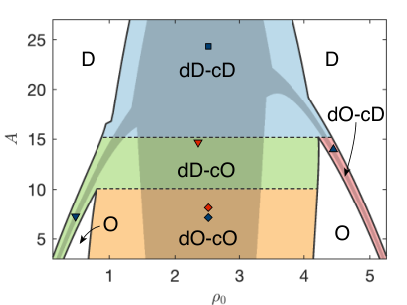
A model with all four phase co-existences.—The linear stability analysis can be applied straightforwardly once and in (2) are explicitly defined. Here, we consider the following model :
| (6) | ||||
| (7) |
with , , and . A microscopic-level (particle based) system that realizes this model could for instance be a polar active fluid with contact inhibition of alignment (e.g., as discussed in Nesbitt et al. 2021) such that its equation of state dictates that it can also phase separates within the homogeneous ordered phase.
For large enough values of , remains negative, and so the system remains in the disordered phase. In this case, instability occurs if , and we expect dD-cD co-existence in this parameter range. On the other hand, as decreases, the range of densities for which the system is in the ordered phase gets wider, and, importantly, is separated from the disordered phase by two instability regions: a dD-cO co-existence to the left and a dO-cD co-existence to the right. Simultaneously, remains negative around . We therefore expect an interesting interplay of distinct phase separations.
In Fig. 2, the instability regions resulting from our linear stability analysis are shown as the shaded area, while the homogeneous disordered (D) and ordered (O) regions are shown in white. We equate the instability region to be within the phase separating region, but to which of the four possible types of phase co-existences?
Since the conserved quantity here is the total mass, can be redistributed as long as the overall density remains the same. Therefore, we can characterize the phases as follows: given any starting point on the phase diagram within the instability region (shaded area in the phase diagram), we extend a horizontal line from that point; the first homogeneous phase encountered to the right (respectively, to the left) will describe the nature of the condensed (respectively, dilute) phase (D or O).
Using the above construction, we see that this particular model contains all four variations of the phase co-existences (Fig. 2). As aforementioned, we report for the first time the existence of a phase co-existence in which both the dilute and condensed phases are ordered. A priori, these two co-moving phases can move either in the same direction or in opposite directions. By directly solving the hydrodynamic EOM numerically SM, this is evidenced in the stationary profiles shown in Fig. 1(b). Besides this particular model, we note that further diversity of phase diagrams are rendered possible by varying the specific definitions of and ; we discuss other interesting cases in SM.
Instability vs. phase separation.—The instability region obtained from a linear stability analysis does not correspond exactly to the whole phase separation region. Indeed, as in thermal phase separation, the instability region in fact corresponds to the spinodal decomposition region, which is always flanked by the so-called nucleation and growth regions on either side Barrat and Hansen 2003; Weber et al. 2019. This is no different here: the actual phase separation boundaries encapsulate the instability regions (Fig. 1). Of course, while the phase separation boundaries (i.e., the binodal lines) for thermal systems in equilibrium can be obtained by analyzing the free energy, e.g., by using the Maxwell tangent method, no free energy exists in our non-equilibrium systems and so the phase separation boundaries will instead be given by the appropriate boundary conditions obtained from the stable steady-state solution of the actual hydrodynamic EOM. This is exactly what we did to obtain the profiles shown in Fig. 1. Specifically, the locations of the binodal lines correspond to the density values of the stationary regions of the condensed and dilute phases (see SM for further details). Finally, we note that both density and active flux profiles obtained numerically display a characteristic fore-rear asymmetry with a steeper fore-front (see Fig. 1). This asymmetry was already observed and discussed in both simulations of microscopic Vicsek-like and active Ising spins models, and their continuum counterparts Solon and Tailleur 2013; Solon et al. 2015a; Solon et al. 2015b.

A multi-critical point.—Besides uncovering the novel dO-cO co-existence regime, our analysis also reveals a potentially novel critical point. To illustrate this (Fig. 3), we consider a polar active fluid system in which there are two generic parameters and that control the phase behavior of the system. Specifically, the system undergoes dD-cD phase separation at high while at small the system is in the ordered phase. In addition, we assume that the second parameter controls the threshold level at which the distinct phase separations happen (Fig. 3). In other words, instead of having additional phase separation due to a negative inside the homogeneous ordered phase as in the previous example, we have here a dD-cD phase co-existence in the homogeneous disordered phase instead.
Now, dD-cD phase separation at criticality belongs to the Ising universality class Partridge and Lee 2019 (but see also Siebert et al. 2018; Caballero et al. 2018). In terms of our hydrodynamic EOM, this critical point corresponds to having in (3). On the other hand, the order-disorder critical point that accompanies critical dD-cO and dO-cD phase separations belongs putatively to a novel universality class () Nesbitt et al. 2021. Therefore, by fine tuning and to zero (indicated by the yellow ball in Fig. 3), these two distinct critical points coincide and the resulting multi-critical point is likely to correspond to yet a distinct universality class for the following reasons: At the linear level around this critical point, the EOM of the active flux is completely decoupled from that of the density field . Specifically, the linear EOM are
| (8) |
where is a Gaussian noise term with a non-zero standard deviation. The fact that does not feature in the linear EOM of is distinct from all known active fluids at the order-disorder critical transition Ginelli and Chaté 2010; Peshkov et al. 2012b; Chen et al. 2015; Großmann et al. 2016; Mahault et al. 2018; Nesbitt et al. 2021; Cairoli and Lee 2019a; Cairoli and Lee 2019b.
Using the linear theory above, we can also identify some interesting novel features of this critical point. To do so, we first perform the following re-scalings:
| (9) | |||||
| (10) |
We can then conclude that the following choice of scaling exponents leave the linear EOM invariant SM:
| (11) |
Applying these linear exponents to the generic nonlinear EOM then indicates that (i) the upper critical dimension is 6 and (ii) the first two nonlinear term that becomes relevant right below are and in the EOM of SM.
Summary & Outlook.—Starting from generic hydrodynamic EOM of polar active fluids, we have unified existing phase transitions and phase separations into a single formulation. In particular, we showed that there are generically four distinct types of phase separations, and illustrated them with a particular model. In doing so, we exhibited a novel co-existence regime: the co-existence of a dilute ordered phase and a condensed ordered phase. We expect that this new phase co-existence will be observed in a microscopic model of active Brownian particles with steric repulsion and velocity-alignment interactions. The numerical study of such a microscopic model and its coarse-graining to link microscopic parameters to the phenomenological coefficients appearing in our EOM is of great interest and will be the subject of further studies. Moreover, we also revealed a putative novel critical behavior. Our work highlights the richness of generic polar active fluid models. The phase behavior can be further enriched by considering variations in other parameters in the EOM. For instance, patterns other than phase separation has been observed when the coefficient in the EOM of the momentum density field (2) becomes negative Wensink et al. 2012. We believe that elucidating these diverse phase behaviors will be a fruitful research direction in the future.
Acknowledgements.
We are grateful to Patrick Jentsch for correcting a mistake regarding the multi-critical point in an earlier version of the paper.References
- Ramaswamy (2010) S. Ramaswamy, Annual Review of Condensed Matter Physics 1, 323 (2010).
- Marchetti et al. (2013) M. C. Marchetti, J. F. Joanny, S. Ramaswamy, T. B. Liverpool, J. Prost, M. Rao, and R. A. Simha, Rev. Mod. Phys. 85, 1143 (2013).
- Bechinger et al. (2016) C. Bechinger, R. Di Leonardo, H. Löwen, C. Reichhardt, G. Volpe, and G. Volpe, Rev. Mod. Phys. 88, 045006 (2016).
- Chaikin and Lubensky (1995) P. M. Chaikin and T. C. Lubensky, Principles of Condensed Matter Physics (Cambridge University Press, 1995).
- Toner and Tu (1995) J. Toner and Y. Tu, Phys. Rev. Lett. 75, 4326 (1995).
- Toner and Tu (1998) J. Toner and Y. Tu, Phys. Rev. E 58, 4828 (1998).
- Toner et al. (2005) J. Toner, Y. Tu, and S. Ramaswamy, Annals of Physics 318, 170 (2005).
- Toner (2012) J. Toner, Phys. Rev. E 86, 031918 (2012).
- Vicsek et al. (1995) T. Vicsek, A. Czirók, E. Ben-Jacob, I. Cohen, and O. Shochet, Phys. Rev. Lett. 75, 1226 (1995).
- Chaté et al. (2008) H. Chaté, F. Ginelli, G. Grégoire, and F. Raynaud, Phys. Rev. E 77, 046113 (2008).
- Grégoire and Chaté (2004) G. Grégoire and H. Chaté, Phys. Rev. Lett. 92, 025702 (2004).
- Thüroff et al. (2014) F. Thüroff, C. A. Weber, and E. Frey, Phys. Rev. X 4, 041030 (2014).
- Solon and Tailleur (2013) A. P. Solon and J. Tailleur, Phys. Rev. Lett. 111, 078101 (2013).
- Solon and Tailleur (2015) A. P. Solon and J. Tailleur, Phys. Rev. E 92, 042119 (2015).
- Gopinath et al. (2012) A. Gopinath, M. F. Hagan, M. C. Marchetti, and A. Baskaran, Phys. Rev. E 85, 061903 (2012).
- Baskaran and Marchetti (2008a) A. Baskaran and M. C. Marchetti, Phys. Rev. E 77, 011920 (2008a).
- Baskaran and Marchetti (2008b) A. Baskaran and M. C. Marchetti, Phys. Rev. Lett. 101, 268101 (2008b).
- Bertin et al. (2006) E. Bertin, M. Droz, and G. Grégoire, Phys. Rev. E 74, 022101 (2006).
- Bertin et al. (2009) E. Bertin, M. Droz, and G. Grégoire, Journal of Physics A: Mathematical and Theoretical 42, 445001 (2009).
- Peshkov et al. (2012a) A. Peshkov, I. S. Aranson, E. Bertin, H. Chaté, and F. Ginelli, Phys. Rev. Lett. 109, 268701 (2012a).
- Peshkov et al. (2014) A. Peshkov, E. Bertin, F. Ginelli, and H. Chaté, The European Physical Journal Special Topics 223, 1315 (2014).
- Bertin et al. (2015) E. Bertin, A. Baskaran, H. Chaté, and M. C. Marchetti, Phys. Rev. E 92, 042141 (2015).
- Cates and Tailleur (2015) M. E. Cates and J. Tailleur, Annual Review of Condensed Matter Physics 6, 219 (2015).
- Tailleur and Cates (2008) J. Tailleur and M. E. Cates, Phys. Rev. Lett. 100, 218103 (2008).
- Fily and Marchetti (2012) Y. Fily and M. C. Marchetti, Phys. Rev. Lett. 108, 235702 (2012).
- Redner et al. (2013) G. S. Redner, M. F. Hagan, and A. Baskaran, Phys. Rev. Lett. 110, 055701 (2013).
- Palacci et al. (2013) J. Palacci, S. Sacanna, A. P. Steinberg, D. J. Pine, and P. M. Chaikin, Science 339, 936 (2013).
- Buttinoni et al. (2013) I. Buttinoni, J. Bialké, F. Kümmel, H. Löwen, C. Bechinger, and T. Speck, Phys. Rev. Lett. 110, 238301 (2013).
- Wittkowski et al. (2014) R. Wittkowski, A. Tiribocchi, J. Stenhammar, R. J. Allen, D. Marenduzzo, and M. E. Cates, Nature Communications 5, 4351 (2014).
- Tjhung et al. (2018) E. Tjhung, C. Nardini, and M. E. Cates, Phys. Rev. X 8, 031080 (2018).
- van der Linden et al. (2019) M. N. van der Linden, L. C. Alexander, D. G. A. L. Aarts, and O. Dauchot, Phys. Rev. Lett. 123, 098001 (2019).
- Peruani et al. (2011) F. Peruani, T. Klauss, A. Deutsch, and A. Voss-Boehme, Phys. Rev. Lett. 106, 128101 (2011).
- Farrell et al. (2012) F. D. C. Farrell, M. C. Marchetti, D. Marenduzzo, and J. Tailleur, Phys. Rev. Lett. 108, 248101 (2012).
- Martín-Gómez et al. (2018) A. Martín-Gómez, D. Levis, A. Díaz-Guilera, and I. Pagonabarraga, Soft Matter 14, 2610 (2018).
- Sesé-Sansa et al. (2018) E. Sesé-Sansa, I. Pagonabarraga, and D. Levis, EPL (Europhysics Letters) 124, 30004 (2018).
- Caprini et al. (2020) L. Caprini, U. Marini Bettolo Marconi, and A. Puglisi, Phys. Rev. Lett. 124, 078001 (2020).
- Jayaram et al. (2020) A. Jayaram, A. Fischer, and T. Speck, Phys. Rev. E 101, 022602 (2020).
- (38) Supplemental Material .
- Dunkel et al. (2013) J. Dunkel, S. Heidenreich, M. Bär, and R. E. Goldstein, New Journal of Physics 15, 045016 (2013).
- Worlitzer et al. (2020) V. M. Worlitzer, G. Ariel, A. Be’er, H. Stark, M. Bär, and S. Heidenreich, “Motility-induced clustering and meso-scale turbulence in active polar fluids,” (2020), arXiv:2011.12219 [cond-mat.soft] .
- Schnyder et al. (2017) S. K. Schnyder, J. J. Molina, Y. Tanaka, and R. Yamamoto, Scientific Reports 7, 5163 (2017).
- Nesbitt et al. (2021) D. Nesbitt, G. Pruessner, and C. F. Lee, New Journal of Physics 23, 043047 (2021).
- Geyer et al. (2019) D. Geyer, D. Martin, J. Tailleur, and D. Bartolo, Phys. Rev. X 9, 031043 (2019).
- Weber et al. (2019) C. A. Weber, D. Zwicker, F. Jülicher, and C. F. Lee, Reports on Progress in Physics 82, 064601 (2019), arXiv:1806.09552 .
- Barrat and Hansen (2003) J.-L. Barrat and J.-P. Hansen, Basic Concepts for Simple and Complex Liquids (Cambridge University Press, 2003).
- Solon et al. (2015a) A. P. Solon, H. Chaté, and J. Tailleur, Phys. Rev. Lett. 114, 068101 (2015a).
- Solon et al. (2015b) A. P. Solon, J.-B. Caussin, D. Bartolo, H. Chaté, and J. Tailleur, Phys. Rev. E 92, 062111 (2015b).
- Partridge and Lee (2019) B. Partridge and C. F. Lee, Phys. Rev. Lett. 123, 068002 (2019).
- Siebert et al. (2018) J. T. Siebert, F. Dittrich, F. Schmid, K. Binder, T. Speck, and P. Virnau, Physical Review E 98, 030601 (2018).
- Caballero et al. (2018) F. Caballero, C. Nardini, and M. E. Cates, Journal of Statistical Mechanics: Theory and Experiment 2018, 123208 (2018).
- Ginelli and Chaté (2010) F. Ginelli and H. Chaté, Physical Review Letters 105, 168103 (2010).
- Peshkov et al. (2012b) A. Peshkov, S. Ngo, E. Bertin, H. Chaté, and F. Ginelli, Physical Review Letters 109, 098101 (2012b).
- Chen et al. (2015) L. Chen, J. Toner, and C. F. Lee, New Journal of Physics 17, 042002 (2015).
- Großmann et al. (2016) R. Großmann, F. Peruani, and M. Bär, Physical Review E 93, 040102 (2016).
- Mahault et al. (2018) B. Mahault, X.-c. Jiang, E. Bertin, Y.-q. Ma, A. Patelli, X.-q. Shi, and H. Chaté, Physical Review Letters 120, 258002 (2018).
- Cairoli and Lee (2019a) A. Cairoli and C. F. Lee, “Hydrodynamics of active lévy matter,” (2019a), arXiv:1903.07565v3.
- Cairoli and Lee (2019b) A. Cairoli and C. F. Lee, “Active lévy matter: Anomalous diffusion, hydrodynamics and linear stability,” (2019b), arXiv:1904.08326v2.
- Wensink et al. (2012) H. H. Wensink, J. Dunkel, S. Heidenreich, K. Drescher, R. E. Goldstein, H. Löwen, and J. M. Yeomans, Proceedings of the National Academy of Sciences 109, 14308 (2012).