Dynamically inflated wind models of classical Wolf-Rayet stars
Abstract
Context. Vigorous mass loss in the classical Wolf-Rayet (WR) phase is important for the late evolution and final fate of massive stars.
Aims. We develop spherically symmetric time-dependent and steady-state hydrodynamical models of the radiation-driven wind outflows and associated mass loss from classical WR stars.
Methods. The simulations are based on combining the opacities typically used in static stellar structure and evolution models with a simple parametrised form for the enhanced line-opacity expected within a supersonic outflow.
Results. Our simulations reveal high mass-loss rates initiated in deep and hot optically thick layers around . The resulting velocity structure is non-monotonic and can be separated into three phases: i) an initial acceleration to supersonic speeds (caused by the static opacity), ii) stagnation and even deceleration, and iii) an outer region of rapid re-acceleration (by line-opacity). The characteristic structures seen in converged steady-state simulations agree well with the outflow properties of our time-dependent models.
Conclusions. By directly comparing our dynamic simulations to corresponding hydrostatic models, we demonstrate explicitly that the need to invoke extra energy transport in convectively inefficient regions of stellar structure and evolution models (in order to prevent drastic inflation of static WR envelopes) is merely an artefact of enforcing a hydrostatic outer boundary. Moreover, the ”dynamically inflated” inner regions of our simulations provide a natural explanation for the often-found mismatch between predicted hydrostatic WR radii and those inferred from spectroscopy; by extrapolating a monotonic -type velocity law from the ”observable” supersonic regions to the invisible hydrostatic core, spectroscopic models likely overestimate the core radius by a factor of a few. Finally, we contrast our simulations with alternative recent WR wind models based on co-moving frame (CMF) radiative transfer for computing the radiation force. Since CMF transfer currently cannot handle non-monotonic velocity fields, the characteristic deceleration regions found here are avoided in such simulations by invoking an ad-hoc very high degree of clumping.
Key Words.
Stars: Wolf-Rayet - Stars: winds, outflows - Stars: mass-loss - Stars: atmospheres1 Introduction
The evolution of stars with initial masses higher than eight times that of the Sun plays an essential role in the chemistry and dynamics of galaxies like our Milky Way (Crowther 2007; Doran et al. 2013; Ramachandran et al. 2018; Prantzos et al. 2018). These massive stars are a vital source of heavy elements and UV radiation, enriching their surroundings through strong radiation-driven winds (Lucy & Solomon 1970; Castor et al. 1975; Puls et al. 2008; Vink et al. 2001; Björklund et al. 2020). In the final evolutionary stages, some of those massive stars become hydrogen-depleted, typically core He-burning progenitors of neutron stars or black holes (Yoon et al. 2012; Groh et al. 2013). Among these are so called classical Wolf-Rayet (WR) stars (Wolf & Rayet 1867), which are characterised by strong spectral emission lines and a high luminosity to mass ratio, , (Crowther 2007). Classical WR stars are distinct from very massive, main-sequence WR stars, which are core H-burning (de Koter et al. 1997; Crowther et al. 2010). Classical WR stars are also different in their composition and evolutionary state from hydrogen-deficient WR central stars of planetary nebula (Todt et al. 2010, e.g.).
As first suggested by Beals 1929, the prominent emission lines visible in WR spectra indicate strong stellar winds with high terminal speeds () and mass-loss rates () (Hamann et al. 2019; Sander et al. 2019). However, while the overall wind properties of massive main-sequence OB-stars (see Puls et al. 2008 for a review) are quite well reproduced by the line-driven wind theory formulated first by Castor et al. 1975 (CAK), this standard theory typically fails to explain the order of magnitude higher mass-loss rates of classical WR stars (Cassinelli 1991; Lamers & Leitherer 1993).
Nonetheless, WR winds are still thought to be radiation-driven, as their high ratio brings them close to the limit at which the acceleration due to radiation balances that of gravity (i.e. close to , for ”Eddington factor” ). In fact, consulting the opacities used in stellar structure calculations which are generally obtained from tabulations computed assuming a static medium (Iglesias & Rogers 1996, e.g.,), the Eddington limit for classical WR stars is already reached in sub-surface layers with temperatures of about . Since convection is highly inefficient in these layers (Gräfener et al. 2012), static models then typically display density inversions and highly inflated stellar envelopes (Ishii et al. 1999; Petrovic et al. 2006; Gräfener et al. 2012; Sanyal et al. 2015). For corresponding stellar evolution calculations, such envelope-inflation is computationally difficult to treat and various numerical ”tricks” are thus typically required to make computations tractable (Paxton et al. 2013; Ekström et al. 2012). This then leads to very hot () and compact () WR stellar surfaces. On the other hand, spectroscopic studies aiming to constrain the WR surface from observationally inferred typically deduce hydrostatic radii that are factors of higher than predicted by such evolution models (Crowther 2007; Sander et al. 2019; Hamann et al. 2019, e.g.,); this mismatch is sometimes referred to as the ”core-radius” problem of classical WR stars.
Rather than retaining a static envelope, breaching the Eddington limit in sub-photospheric layers can initiate an optically thick supersonic outflow. Nugis & Lamers 2002 and Grassitelli et al. 2018 suggested that WR mass-loss rates can be computed simply by considering only the conditions at the point where the sonic speed is reached (at , since gas pressure terms typically are very small in comparison). Using the OPAL tables of Rosseland mean opacity (Iglesias & Rogers 1996), Ro & Matzner 2016 showed that supersonic velocities are indeed found in deep sub-photospheric layers, but that a successful wind solution that could bring the initiated mass flux to infinity could not be found.
However, these models neglect the strong enhancement of the line-opacity expected in a supersonic outflow. Previous modeling attempts including the Doppler effect in the line opacity calculations have either relied on a pre-assumed fixed velocity field to solve for the mass loss (Lucy & Abbott 1993; Springmann 1994; Springmann & Puls 1998; de Koter et al. 1997, e.g., see), or attempted an iterative (assuming time-independence) solution toward a self-consistent velocity field and mass loss (Gräfener & Hamann 2005; Sander et al. 2020; Sander & Vink 2020). The latter models have used comoving-frame (CMF) radiative transfer for the calculation of . Such CMF transfer is a computationally intensive numerical technique that requires the velocity field to remain smooth and monotonic (see, e.g., discussion in Sander et al. 2020). Moreover, all these previous studies of classical WR outflows have been performed in the steady-state limit.
In this paper we present a first attempt to build a model that addresses both (dynamic) envelope-inflation and line-driving, using a ”hybrid” opacity approach based on combining the opacities used for static stellar structure calculations with a simple variant of the standard parameterisation for line-opacities in supersonic flows. This formalism then allows for computation of both steady-state and time-dependent WR wind structures. The organization of the paper is as follows: In Section 2, we describe our basic physical set-up . We present dynamical models in the steady-state limit and compare these to corresponding static calculations in Section 3. Then in Section 4 we compare these steady-state models to full time-dependent radiation-hydrodynamical simulations of ”dynamically inflated” WR outflows. In Section 5 we discuss our results and some open questions regarding WR stellar outflows, and finally we summarise our results and provide an outlook for future work in Section 6.
2 Physical model
We describe the WR wind outflow by the appropriate hydrodynamical equations of mass and momentum conservation assuming spherical symmetry:
| (1) |
| (2) |
Here , and are mass density, velocity and gas pressure, where is gas temperature, is the Boltzmann constant, is the mean molecular weight, and is the mass of the hydrogen atom, is the gravitation acceleration for a constant stellar mass and
| (3) |
is the acceleration due to stellar radiation, for radiation flux and flux weighted opacity (”mass absorption coefficient”) in . Using the Eddington factor we can also write the equation of motion (e.o.m) as:
| (4) |
The Eddington ratio can be expressed as:
| (5) |
for a stellar luminosity . In this paper, we assume that the radiative luminosity remains constant throughout the outflow. This means that, we neglect a term corresponding to the work of the radiation field against gravity. We can estimate the corresponding expected luminosity variation by computing the photon-tiring parameter (Owocki et al. 2017), which is the ratio of the stellar mass loss to the maximum amount of mass loss that the stellar luminosity can drive, , where is the ”core radius” defined at the fixed lower boundary. Taking the stellar parameters used throughout this paper, , , and a typical order of magnitude mass loss, , one gets
| (6) |
which demonstrates that the luminosity variation is only a marginal effect for the cases considered in this paper.
In practice, especially for time-dependent dynamical computations (with possibly non-monotonic velocity fields) it is not computationally feasible to derive the temperature structure, e.g., from radiative equilibrium by means of full solutions to the frequency dependent radiative transfer equations. To simplify, we therefore follow the common approach of replacing the full energy equation by the Lucy 1971 analytic radiative equilibrium model for a grey, spherically symmetric, diluted atmosphere, however, replacing the grey opacity by the actual flux weighted (Lucy & Abbott 1993, e.g., see). This allows us to write the temperature structure as:
| (7) |
where is a ”core effective temperature”, defined here from the lower boundary set at , is the Stefan-Boltzmann constant, is the dilution factor, and is the spherically modified optical depth
| (8) |
Here again the radius of our fixed lower boundary is used as a scaling radius for the spherically modified optical depth scale. This is similar to the WR models by Sander et al. 2020 who also define their stellar radius from the hydrostatic lower boundary. It is different, however, than, e.g., Sundqvist et al. 2019 who set the reference radius for the temperature structure in their O-star models at a photospheric radius . An argument against using as a scaling radius for optically thick WR winds is, however, that , such that the geometric dilution of the radiation field would be neglected for large parts of the outflow (Nugis & Lamers 2002, see also discussion in ). In principle, the explicit choice of the reference radius will affect the temperature structure throughout our models. However, test-calculations have shown that this is a quite marginal effect for the resulting mass loss and velocities of the simulations considered in this paper. In any case, to facilitate comparison with other models we also introduce a ”stellar photospheric effective temperature” at this photospheric radius . Since the definition of a stellar photosphere in a spherically diluted stellar envelope is non-trivial11 1 For example, in Section 3.6 the stellar photoshere is located at the surface in the radiation diffusion approximation, rather than the typically assumed photoshere location at the surface. and depends on the specific computation of the temperature structure, we here simply approximate
| (9) |
such that the photospheric and core effective temperatures and radii are related through
| (10) |
For given stellar parameters , , and , and a known variation of , Eqs. 1-8 form the basic system of coupled differential equations under investigation in this paper. In general, is a complicated function that depends on chemical composition, density, temperature, velocity and redial position of the absorbing and emitting gas. In this study, we focus on two cases. First, we consider static opacities such as those used for stellar structure and evolution computations (Ro & Matzner 2016, see). Due to the high continuum optical depth of WR outflows, conditions in the wind launching regions resemble those of radiation diffusion, allowing us to replace the flux-weighted opacity with a Rosseland mean, and so to utilise standard OPAL tables for the opacity-mapping as a function of and (Iglesias & Rogers 1996). However, since these tabulations ignore the influence of Doppler shifts on the line-opacity (Sander et al. 2020, which are critical for WR wind driving, e.g.,) we will also consider a ”hybrid-model” accounting at least approximately for this effect. More specifically, we will use a CAK-like parametrisation to add the cumulative force from an ensemble of spectral lines to the OPAL tables (see, Section 3.3).
3 Steady-state approximation
To build physical insight we first examine a simplified steady-state case. Equations 1 and 4 are then written as:
| (11) |
| (12) |
for an isothermal sound speed . Equation 11 defines the spherically symmetric mass loss rate . Here we assume corresponding to a fully ionised helium plasma.
It is commonly believed that the winds of WR stars are initiated in the deep sub-photospheric layers where the gas temperature is . In this temperature region, due to iron recombination, a significant increase of the Rosseland mean opacity is observed, sometimes called the ”iron opacity bump”. A simple comparison of scales reveals that throughout the supersonic wind outflow the first two terms of the r.h.s. in Eq. 12 are much smaller than the radiation and gravitation terms, so that we can approximate the e.o.m with
| (13) |
Here, the sound-speed term on the l.h.s. is retained in order to enable a mapping of the supersonic solution onto the subsonic part.
3.1 Boundary conditions
Equations 7-13 impose a two-point boundary value problem, with boundaries at and at22 2 for numerical computations the outer formal boundary is simply replaced by a maximum radius .
The inner boundary at is defined to be a sonic-point, with , where is defined to be the sound-speed at this sonic-point. As can be seen from Eq. 13, this implies . Below the sonic point as the velocity rapidly diminishes from its sonic point value inwards, the density structure is well approximated by the hydrostatic solution (Ro & Matzner 2016; Grassitelli et al. 2018, e.g. see). In contrast, in the super-sonic part, the density structure diverges from the structure given by the hydrostatic solution. As such, we initiate the calculation at the sonic-point and only consider the super-sonic part of the outflow, assuming that the sub-sonic region still can be described by hydrostatic equilibrium. The tabulated OPAL opacities can then be used to locate points for which , constraining the lower boundary density as a function of temperature. In this way, the range of possible mass-loss rates is set as a function of the lower boundary temperature.
The outer boundary is set by requiring that the wind temperature decreases sufficiently at large radii. Replacing density with the mass-loss rate using Eq. 11, the spherically modified optical depth (Eq. 8) is used to compute the temperature structure according to Eq. 7. We compute the optical depth at the outer boundary by radially integrating Eq. 8 in , assuming a terminal velocity and , where is the Thompson scattering mass absorption coefficient. The outer boundary temperature is then set by the maximum between applying in Eq. 8 and a floor value, which is typically set to a few tenths of the stellar effective temperature (Puls et al. 2005; Sundqvist et al. 2019, see). By matching the inner and outer boundary constraints, we uniquely constrain the wind structure. In turn this then sets the unique mass-loss rate of the model from the range of possible solutions at the lower boundary.
3.2 Energy requirement
Additionally, for wind material to escape the stellar potential, the global energy requirement must be satisfied, which means that the integrated mechanical energy of the wind has to be positive. Taking the supersonic limit in Eq. 13 yields:
| (14) |
Here is the initial velocity and is the escape velocity from . The first term on the r.h.s. corresponds to the work done by the stellar radiation and the second term is the work done by gravity. We can then introduce as the net energy change in units of :
| (15) |
For the wind to escape to , this net energy change has to be positive, i.e. . Alternatively, we can also introduce the ratio of kinetic to core potential energy as a square of the velocity to core escape velocity ratio:
| (16) |
which goes to as so that by construction we require in order to escape.
3.3 Failed Winds in the static opacity limit
Let us first investigate the possibility of driving the stellar outflow in the static opacity limit, i.e. the limit in which we only consider OPAL opacities, thus neglecting the Doppler effect; (Ro & Matzner 2016, see also). To set up the problem, we choose the stellar mass and the core radius (as given in Table 1) such that they roughly represent the average value of the mass-to-radius ratio of the observationally inferred WR stellar population from Hamann et al. 2019 and Sander et al. 2019. The luminosity is then set such that the resulting Thompson scattering Eddington ratio , which also corresponds approximately to the observationally inferred average (Hamann et al. 2019; Sander et al. 2019). All models presented in Sections 3 and 4 of this paper use these stellar parameters, and also the OPAL tables for solar metallicity and composition by Grevesse & Noels 1993. This set-up then gives a range of possible sonic-point values of such that the condition is fulfilled (see Fig. 1(a)). These points are used as a single point boundary condition, after which forward integration from the sonic-point is carried out. The results of these integrations for various fixed mass-loss rates are shown in Fig. 1(a). The figure displays a colour map of with the temperature on the abscissa and the ratio between the radiation pressure
| (17) |
and gas pressure on the ordinate (the ratio is a proxy for the density). The integration-curves show the density and temperature structure for the different cases, starting from various positions on the curve at the inner boundary and extending outwards. Figure 1(b) then shows the corresponding net gain of kinetic energy (Eq. 16), demonstrating that after an initial acceleration and increasing velocities, all of the curves start to decelerate until eventually reaching zero velocity and so terminating the outward integration (some solutions had to be formally terminated before actually reaching zero velocity, due to numerical difficulties in the steep deceleration region). This indicates that none of the potential solutions starting from the curve are able to escape the stellar gravitation potential. These results are consistent with Ro & Matzner 2016, who also found that OPAL opacities were not able to sustain a radiation-driven mass loss initiated in the deep layers around the iron-bump, and indicates that an additional source of opacity is required, raising the question of a ”missing force”.


3.4 Missing force
The natural candidate for the missing opacity source discussed above comes from the cumulative effect of spectral lines due to the Doppler effect. To estimate this we use the CAK parametrisation for a distribution of spectral lines, using here a simple approximation of taking the absolute value of the velocity gradient:
| (18) |
where is an effective strength of the line ensemble (Gayley 1995), and sets the CAK line distribution power index. In reality, once regions where arise, it is possible for a photon proceeding from the stellar core to be Doppler shifted into resonance with the same spectral line at multiple locations in the outflow, thereby requiring a fully non-local computation of the line acceleration. As discussed further below, this could (in principle) be handled in a more self-consistent manner by e.g. Monte-Carlo (MC) line-force calculations. In this initial study, however, we opt for a simpler approach, in order to make time-dependent simulations feasible as well. Two possible approximations that can be taken then are to either take the absolute value of the velocity gradient or use . The first approach estimates (approximately) an upper limit to the CAK-like force in regions with negative velocity gradients, whereas the second approach would correspond to a lower limit. As most previous studies of line-driven dynamical flows have used (e.g., in investigations of line-driven winds from rapidly rotating stars, Petrenz & Puls 2000, and around discs, Proga et al. 1998; Kee et al. 2016), we follow this standard approach in this paper. However, test computations using instead the lower limit show that although some details of the radiation force profile then are changed, none of our conclusions are affected. With this approximation, using Eq. 18 for then accounts for the force from spectral lines in supersonic regions, while handles the force from the continuum and spectral lines in the static limit. As such, the total radiative acceleration can be simply estimated by the sum of the CAK-like contribution and the static OPAL opacities, .
Let us note here directly that the CAK line-force is originally derived for application in winds that are optically thin for continuum radiation. In the lower layers of the dense WR outflows considered here, this will typically not be the case. A more rigorous treatment would then need to take into account also the change in continuum intensity by solving the transfer equation for line+continuum opacities. While approximations for the diffusion limit exist (Gayley et al. 1995) no general formalism has been developed. As such, in this first study of WR wind dynamics we opt for the simple radial streaming CAK-form above.
Furthermore, due to the explicit dependency of the CAK line-force on the sonic-point is now formally not a critical point (see Castor et al. 1975). However, our iteration scheme circumvents this issue by always applying the velocity gradient from the previous iteration, meaning that technically is no longer an explicit function of . Nevertheless, since we require to be converged between iterations the corresponding feedback upon is still (implicitly) accounted for. The agreement between the converged structures of these steady-state models and the time-dependent simulations presented in the next section brings further support to this method.
A key question then becomes whether also has a significant impact on the conditions at the optically thick lower boundary at the sonic point. Assuming typical O-star values , (Puls et al. 2000, e.g.,), approximating the velocity gradient33 3 We define as the maximum velocity found for the given fixed mass loss in the static opacity limit. as , and using the mass density and velocity computed in the static opacity limit for , we find the Eddington ratio for the CAK force at the lower boundary to be . Such a small contribution from the CAK force is not surprising due to the high density at the lower boundary44 4 The numerical simulations presented in Section 3-4 a posteriori confirm the simple order of magnitude estimate made here, showing explicitly that the force contribution from the CAK-like opacities near the lower boundary indeed is very small for our considered cases (see e.g. Fig. 3(c)). This thus resolves some potential issues of our basic approach (simple summation of OPAL and CAK-like opacities) regarding ’double-counting’ the effect of spectral lines in the static limit. (, with ). However, from test-calculations it turns out that although the CAK contribution indeed increases as we move outwards in the wind, a simple model with constant , is still not able to provide the force necessary to achieve a positive total wind energy and so drive the wind to infinity (see previous section).
There are, however, several indications that the line-force in the outer winds of classical WR stars indeed might be significantly enhanced as compared to O-type stars. For example, the independent MC line-force calculations by Lucy & Abbott 1993 and Springmann & Puls 1998 both find global momentum rates for WR stars that exceed those of O-stars by an order of magnitude or more. In these MC computations, the outer-wind enhancement of the line-force stems from the decreasing level of ionisation with increasing distance from the star in the optically thick WR outflows. Due to this shift from high-to-low ionisation stages as photons move outwards in the wind, ”new” spectral lines become available for photons to interact with. As these new lines have different interaction frequencies than those previously available in the inner wind parts, this means that the line-frequency gaps typically observed for the nearly constant (”frozen-in”) ionisation conditions of optically thin O-star winds are effectively closed. This then leads to ”photon-trapping” (Lucy & Abbott 1993) and efficient multi-line scattering, which significantly increases the line force.
To mimic the effect of an outer wind line-force enhancement, we introduce here a simple spatial variation , which increases the CAK force away from the star by a modest decrease of . To this end, we assume as a piecewise linear function with a constant from the lower bounder to and a constant from to the outer boundary, interpolating between the two values in the range . This then allows the wind outflow initiated at the lower boundary to achieve positive total energy, and so be sustained until the upper boundary. While the specific treatment of is done here in an ad-hoc manner, the overall assumed form is quite consistent with the multi-scattering line-force enhancement found in the MC line-force computations for a CAK-like spectral line distribution by Springmann 1994. The approximate values of that correspond to the line-force computed by Springmann 1994 are given in Fig. 2 as black asterisks, with the as adapted in the standard model of this paper over-plotted as a solid line.
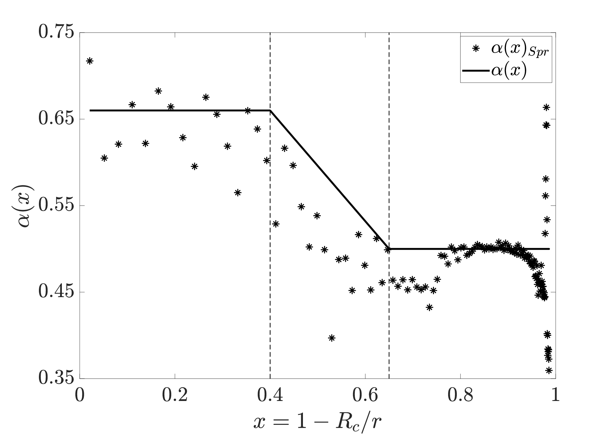
The figure shows that the order of magnitude outer-wind line-force enhancement applied here indeed is on the same order as that found in these MC calculations.
We note, however, that the Springmann 1994 calculations were performed only for parameterised (monotonic) -type velocity laws. As such, there is not a complete one-to-one correspondence between the spatial and velocity scales in these MC calculations and those of the present paper. Nonetheless, the overall similarity with the very simple radial dependence of the parameter adopted here is encouraging. In a follow-up work, we plan to couple the hydrodynamic simulations presented here directly to such MC computations, building on the method developed by Puls et al. 2000 for proper estimation of occupation numbers, and accounting fully for multi-scattering effects as well as non-monotonic velocity fields.
As outlined in details in the following sections (for our standard values listed in Table 2) the formalism outlined above gives rise to ”dynamically inflated” wind solutions, where the structure in the optically thick deep layers near the iron bump is primarily governed by but where takes over the driving in the diluted outer regions. This then causes a typical wind structure that is characterised by a high mass-loss rate ignited from the lower boundary, a slow (end even partially negative) acceleration of the deeper layers, and a rapid re-acceleration of the outer wind. As such, the typical velocity laws we find not only drastically deviate from the standard -type laws assumed by most atmospheric models, but they also contain a significant region of negative acceleration (Pauldrach et al. 1993, see also fig. 14 in).
3.5 Dynamically inflated steady-state model
Based on the ”hybrid” formalism introduced above we can now numerically solve Eqs. 7-13, iterating toward convergence using a simple scheme based on Runge-Kutta integrations. As discussed in Section 3.1, to constrain the mass-loss rate it is critical to here take into account the two-pointed boundary value nature of the problem. At a basic level, every iteration is performed using two steps: i) an inside-out integration , where the velocity, density, and temperature structure are computed, followed by ii) an outside-in integration updating the temperature structure using the correct boundary condition from the optical depth found in the first step. The mass-loss rate is then updated for the next iteration by finding the correct location on the curve at the lower boundary, using the updated temperature structure from the outside-in integration.
Using this scheme, Figure 3(a) shows the final, converged temperature profile for our standard stellar parameters (Table 1) and choice of line-force parameters (Table 2). The final (also converged) mass-loss rate for the model is .
In addition to a high predicted mass-loss rate, the solution displays a non-monotonic velocity field. The resulting velocity profile shown in Fig. 3(b) can be split into three basic regions: 1) an initial acceleration from the core followed by 2) stagnation and even a deceleration part (and so a negative velocity gradient, marked with crosses in the figure), and 3) an outer region of fast re-acceleration to outflow velocities . The distinct behaviour of these three regions can be understood via the different contributing parts of the total radiation force.


Figure 3(c) illustrates this, plotting the individual contributions of OPAL and CAK-like opacities to the total radiative acceleration. From the figure, on one hand, it is clear that in the inner regions the radiation force is dominated by OPAL opacities and the CAK-like contribution is small; indeed, the sonic point conditions at the lower boundary can here be quite well approximated using only OPAL opacities (i.e., neglecting any influence from the Doppler-shift enhancement of line-opacities). On the other hand, in the outer regions becomes the dominant part, causing a re-acceleration of the flow and setting a high terminal wind velocity. This re-acceleration ensures that the energy requirement of Eq. 15 is satisfied. As such, it is this part that ultimately allows the wind to be sustained all the way to the outer boundary, in contrast to the ”failed outflow” and fallback seen in the previous section.
To explore the influence of different opacity contributions on the mass loss of the model, we explore the logarithm of the spherically modified optical depth (Eq. 8) as a function of radius in Fig. 3(d). The dashed vertical line marks the location of the stellar photosphere defined by Eq. 9. (Note, however, that at the photosphere as is used as a scaling radius in Eq. 8.) For most stars, this photospheric radius serves as the hydrostatic stellar radius; by contrast, for the WR stars examined in this paper, the photosphere is located well in the outflowing regions. Inspection of Fig. 3(d) shows that the majority of is accumulated within few stellar radii in the regions dominated by OPAL-opacities, thus the converged lower boundary temperature (and thus the mass-loss rate) is primarily controlled by .
Inspection of the density distribution in Fig. 3(e) further clarifies the terminology ”dynamic inflation”. In this figure, we have again identified the location with a vertical dashed line. The figure shows a relatively slow decline of the density in the sub-photospheric parts, which is somewhat reminiscent of the profiles seen in hydrostatic stellar models near the Eddington limit that undergo envelope inflation (see further below). But unlike such static inflation models, the simulations here allow for a velocity field to develop; the low-density envelope now represents a ”dynamically inflated” star.
3.6 Comparison to static inflation
For the same lower boundary conditions as adopted above, we can also compute static models. This can then serve as a direct comparison between the dynamic inflation found in the models above, and the static inflation that often occurs in stellar structure models neglecting the term in the e.o.m. (and so assuming a hydrostatic stellar envelope throughout, e.g., Petrovic et al. 2006; Gräfener et al. 2012).
To construct such static models, we simply set in our steady-state e.o.m. above. Introducing a column mass
| (19) |
we write the resulting equation of hydrostatic equilibrium as:
| (20) |
We further simplify the temperature calculation by assuming radiative diffusion in these optically thick hydrostatic layers:
| (21) |
for a radiation pressure according to Eq. 17. Combining the equations for gas and radiation pressure, one obtains
| (22) |
where now throughout the complete model.
This set-up imposes a similar two-point boundary value problem as previously analysed. To provide a fair comparison with those dynamical simulations, we assume the same lower boundary radius as before and re-use the lower boundary temperature found from the converged hydrodynamic steady-state model presented above. However, at this inner boundary we now impose as would lead to non-zero gas pressure at (Gräfener et al. 2012, see also Section 2.2 in). The outer boundary conditions for gas and radiation pressure (i.e., density and temperature) are also set up in the same way as before. Assuming for the region , we may integrate the hydrostatic equations to estimate the temperature and the density at the outer boundary . This fixes the ”effective temperature” and the spherically modified optical depth scale of these hydrostatic (HS) models, requiring that the outer boundary always satisfies . Thus in this model, the ”stellar photospheric radius” is defined as
| (23) |
for the corresponding ”hydrostatic effective temperature”
| (24) |
quite analogous to how these quantities typically are defined in static stellar structure and evolution models.
These boundary conditions are used to numerically solve the new set of equations from the outer boundary inwards. A consistent solution is obtained by shooting for the fixed inner boundary temperature and radius, varying the stellar photospheric radius and assuming inner-boundary values as discussed above. In this way we obtain static envelopes corresponding directly to our previous dynamic models. The right panel of Fig. 4 shows the predicted densities for static models with different assumed55 5 For the fixed stellar mass and electron scattering mass absorption coefficient the variation of is equivalent to the variation of (Gräfener et al. 2012, for comparison see Fig. 1 in). These densities are then compared to those of the steady-state computation in Section 3, for which .


We note directly that in the static case an extended region of low density is formed. The photospheric radius of this ”inflated envelope” is extremely sensitive to , with growing notably as is increased . For the static model with highest assumed , we already find a large accompanied by a relatively cool effective temperature ; further increasing causes the inferred photospheric radius to inflate to increasingly unrealistic, extremely large values. For the that we use in our dynamic models we find and . The reason for the inflation here is the same as in the models by Petrovic et al. 2006 and Gräfener et al. 2012. Basically, it is related to the fact that for high values of the integration moves along a curve, forcing the density to remain low and almost constant over a large radial extent. Since enough column mass (or equivalently optical depth) still has to be accumulated in order to meet the lower boundary condition, the only way the star can react is by expanding in radius (Owocki 2014, see also discussion in). Comparing this now to our dynamic solutions shows that, for the same , inclusion of the dynamical terms reduces the inflation somewhat. Nonetheless, still lies very far away from the core in such outflow models of dynamically inflated envelopes; indeed, for our standard we obtain and . Such a close agreement of photospheric radii in dynamic and static models is however not generally found. Namely, a very small increase to in the static model leads to an order of magnitude increase of the star’s photospheric radius (see Fig . 4), in contrast to the dynamic model where this barely affects the location of .
The analysis above assumes that all luminosity is carried by radiation. In stellar models, the strong increase in opacity around the iron-bump will typically lead to an onset of convection, such that . In principle, this may alleviate the inflation by allowing a portion of the luminosity to be carried by convection, lowering the effective . However, for the conditions prevailing in WR stars convection in these near-surface layers should be very inefficient. Following Gräfener et al. 2012, an upper limit to the fraction of the total stellar flux that can be carried by convection is:
| (25) |
This means that for the considered in this paper, less than a percent of the total luminosity will be carried by convection.
This convective inefficiency is confirmed by the computation of WR stars using the stellar structure and evolution code package MESA (Paxton et al. 2019). Namely, using the standard mixing-length theory (MLT) prescription for convection shows that such stellar structure and evolution computations66 6 Detailed description of these models as well as Input files to reproduce our MESA simulations are provided at https://doi.org/10.5281/zenodo.4054811 indeed undergo similar inflation in the WR stage as seen here in Fig. 4. However, in these stellar evolution simulations envelope inflation and the associated density inversions often imply prohibitively short time-steps within the model-calculations. To prevent this from happening, such stellar models often invoke an additional energy transport that is far greater than that implied by the upper-limit estimate of above (Paxton et al. 2013, see, for example, the so-called MLT++ prescription in MESA, Section 7.2 in). This then forces to always be low enough such that the calculation can proceed.
To mimic these ”tricks”, in the next step we artificially reduce by introducing . Then using in Eq. 20, while computing the radiation pressure from the total luminosity in Eq. 21, we solve the differential equations exactly as above. By then assuming different ratios for the same fixed total luminosity, we can directly compare dynamic and static inflation models with and without such a reduction in radiative luminosity. Analogous to the left panel, the right panel of Fig. 4 shows the radial density structure of a case with reduced radiative luminosity (solid black line), comparing this to the original case (solid-marked line). The ratio of here is chosen such that the stellar envelope no longer experiences a density inversion. The figure demonstrates clearly that the two solutions have vastly different radial scales; while the original model had and , the model with reduced radiative luminosity has a very hot and a photospheric radius that lies less than a percent above the core .
The reason for these drastically different stellar photospheric radii is the same as described earlier; including an additional (artificial) energy transport reduces the effective , so that a dense exponential atmosphere with small scale-height is formed. This then avoids inflation and density inversions, and the upshot is a hot and compact WR stellar surface. This is a good example of how envelope inflation and density inversions are often avoided in stellar structure computations by reducing well beyond the limits implied by standard convective energy transport.
A key result of our analysis here is thus that such ”tricks” of the near-surface regions in WR stars are necessary only because of enforcing a hydrostatic solution. As shown above, when including the dynamical terms the stellar envelope will instead quite naturally develop a ”dynamically inflated” outflow region.
4 Time-dependent numerical hydrodynamic simulations
The previous section presented calculations in the steady-state limit, using various degrees of approximations for solving the dynamical (and static) equations. Building on the same basic formalism, this section now presents full time-dependent numerical hydrodynamics simulations for spherically symmetric WR wind outflows. A key objective is to examine whether such time-dependent simulations relax to similar solutions as the simplified steady models of Section 3.
The hydrodynamic simulations are performed using the finite volume code MPI-AMRVAC (Xia et al. 2018) to solve Eqs. 1, 4, and 7. We use the HLL solver (Harten 1983) with a MINMOD flux limiter (van Leer 1979). The radiative acceleration is computed as in Section 3.3 by summing up the contributions from OPAL and CAK-like opacities, . Here the OPAL contribution is trivially obtained from the local density and temperature, and the CAK contribution from a simple central finite difference scheme applied to Eq. 18. To avoid information propagating over multiple cells in a single integration we further limit the integration time-step by:
where is the time-step set by the standard Courant-Friedrichs-Lewy condition (Courant et al. 1928), and the width of one numerical cell.
As Eq. 7 is not the standard way of computing the energy balance in MPI-AMRVAC we have implemented an additional routine to handle this. In this subroutine the optical depth Eq. 8 is first computed by trapezoid integration starting from the outer boundary , setting as before, inwards to . The radial temperature structure is then updated at each hydrodynamical time step according to Eq. 7. For simplicity, we here define to always be at the lower boundary of the simulation.
4.1 Initial and boundary conditions
Analogous to our steady-state simulations, we define the outer boundary to be located at some radius and use the same optical depth and temperature conditions as described in the previous section, Eq. 7 and the pre-specified minimum temperature (see above). As in e.g., Driessen et al. 2019, the numerical outer boundary conditions on the velocity and density are set by simple extrapolation from the outer most points of the simulation grid. To properly resolve the sonic-point we set the inner boundary to a lower radius than the expected sonic-point , i.e. now . At this we then fix the lower boundary density and allow the velocity to adjust to the overlying wind conditions (Owocki et al. 1988, see, e.g., ). is initially estimated from our corresponding steady-state models by simply assuming hydrostatic equilibrium below the sonic-point. The stellar mass and luminosity still are as in Table 1.
The initial wind condition is an analytic outflow structure, in the form of a simple ”-law”:
| (26) |
where the terminal velocity , and are derived from a simple assumed . The parameter sets the minimum initial velocity at , here chosen such that . The equation of continuity then directly provides the initial density structure. Finally, the initial temperature structure is computed from Eq. 7 with the opacity set according to the assumed input from above. Using these initial and boundary conditions, numerical time integration is carried out until the wind relaxes to a (quasi) steady state. We, however, note that the results of our simulations are not sensitive to these assumed initial conditions.
4.2 Time dependent dynamic inflation model
Starting from the initially assumed structure the wind outflow gradually relaxes to a hydrodynamically consistent structure. The velocity-relaxation is displayed in Fig. 5 as a surface plot, where along one horizontal axis the physical time of the simulation is shown and along the other the radius in . The vertical axis then measures velocity (in ). At the initial velocity structure, , is visible, however as time increases this -type structure gradually evolves toward the three-phased velocity profile discussed in Section 3.5. Around at the simulation has relaxed to a state very similar to that found in our corresponding steady-state model (Section 3.5).

Running the simulation for in total , figures 6(a) and 6(b) show the Eddington ratio and the velocity profile of the final time-step. From Figure 6(a) we observe that, just as in the steady-state model, the CAK-like force near the lower boundary on average only has a small contribution to the total force; contrarily, near the outer boundary, it is dominant. The radiation force from the OPAL contribution has the opposite behaviour, dominating at the sonic-point and in the inner regions, but becoming secondary in the outer parts. This then again leads to a velocity profile (solid line in Fig. 6(b)) with a non-monotonic behaviour, which clearly can not be fit with the simple -type velocity law assumed in the initial conditions (dotted line).
This velocity profile can be directly compared to that found in our corresponding steady-state model, illustrated by the dashed line in Fig. 6(b), which shows close agreement between the two. The mass loss of the time-dependent model is , which also agrees well with the mass-loss rate of from our steady-state model (see Section 3). In this way, our time-dependent models demonstrate that the ’dynamically inflated’ solution discussed in the previous section indeed works as a stable attractor for the stellar wind envelope, confirming our basic conclusions regarding a wind outflow controlled primarily by OPAL opacities in the inner regions, and by the CAK-like force in the outer. The small differences in velocity magnitude and mass loss between steady-state and time-dependent models are mainly related to differences in setting the lower boundary. In steady-state computations we define the sonic-point to be exactly at the lower boundary, whereas in time-dependent computations it is allowed to self-adjust so that the sub-sonic part is also resolved.


4.3 dependency on CAK
A general finding of our baseline simulations in Sections 3 and 4 is that (as long as the wind can escape), the mass-loss rate is primarily controlled by the conditions in the lower wind; in contrast, the terminal wind speed is controlled mainly by the outer wind conditions. Moreover, while it has turned out that a steady-state model, such as the one presented in Section 3, is quite difficult to converge, the time-dependent simulations of this section are computationally somewhat easier to handle.
Therefore, we have used our time-dependent set-up to further explore the impact of the CAK-like force parameters on the predictions of and . We investigate the impact of these parameters by varying only and , however we point out that comparable effects could also be achieved by instead introducing corresponding radial variations of the second line-force parameter . To this end, we test a range of values and , corresponding roughly to the scatter of observed in the MC simulations displayed in Fig. 2. The results of these tests are summarised in Tables 3 and 4, along with the mass-loss rates and terminal velocities found for the different model-runs. In addition, we also tested variations in the spatial position of the to transition for the standard CAK force parameters in the range . However, for these tests, no significant influence on the mass-loss rates of the models have been observed. Therefore, the following subsections focus exclusively on varying the values of and .
4.3.1 Dependency on
As is the prevalent driver in the outer wind, one might initially expect a similar dependence of the mass-loss rate on as given by the standard CAK model. The CAK expression for the mass-loss rate , typically derived from critical-point analyses for in the radial streaming limit, is:
| (27) |
From this expression, it directly follows that increases steeply if is decreased while keeping all other parameters constant. However, it can be seen from Table 3 that in our models varies only marginally across the range of considered values. This distinguishes these optically thick WR simulations from standard CAK-type models applied to the optically thin winds of O-type stars. We further confirm the finding from the steady models that if is increased too much, the line force becomes insufficient to sustain the outflow. This happens because the line acceleration in the outer wind must be sufficient to prevent fall-back of the mass-loss initiated at the Fe-opacity bump. That is, the line acceleration must provide enough additional energy such that the previously introduced condition is fulfilled. As alluded to above, the CAK mass-loss rate formula cannot be directly used to predict the mass loss of this hybrid model. Nevertheless, the limiting value of that can sustain the wind can be estimated by inverting the above equation, solving for the at which the CAK mass-loss rate equals that of our actual model. For the given model with , one finds . The results of our numerical simulations, summarised in Table 3, indeed suggest that this provides a reasonable estimate for the limiting value.
This is also supported by closer inspection of the simulations with , which results in a flattening of the wind velocity profile as . With a further increase to , we find that the CAK-like force is unable to keep up with the mass flux initiated at the lower boundary. In the 1D simulations presented here, this then leads to a similar ”failed wind” situation as discussed in the previous section; we discuss potential implications of this behaviour for multi-dimensional versions of our simulations at the end of the next section.
Finally, as summarised in Table 3 the terminal velocity indeed is very sensitive to small changes of . Overall, this thus suggests that within this formalism, and are determined quite independently. As discussed further in Section 5.2, such a basic decoupling of and indeed seems to be supported by observational data of WR winds (Hamann et al. 2019; Sander et al. 2019, e.g. see). On the other hand, this result also seems to contradict that of the most recent study from Sander & Vink 2020, who find a correlation between and . We further discuss possible reasons for this in Section 5.4.
| 0.48 | 0.66 | 1.59 | 4.60 | 2765 |
| 0.50 | 1.64 | 2.70 | 2063 | |
| 0.52 | 1.68 | 1.66 | 1279 | |
| 0.53 | — | 1.33 | — | |
4.3.2 Dependency on
In contrast to , has little to no effect on determining the terminal velocity of the outflow. Nevertheless, it can affect . This is illustrated in Table 4, where a modest increase in is found for decreasing values of . We note, however, that again the magnitude of the mass loss variation is small in comparison to that seen in CAK-type wind models of optically thin O-stars.
This rather weak dependence on the CAK force stems from the fact that the dominant contribution to the total radiation force comes from the OPAL opacities in the regions near the stellar core (see also Section 3). At the sonic point for , we find and for the we find , which is much lower even than our initial order of magnitude estimate in Section 3.4. This further supports that the CAK force has a negligible contribution at the sonic point. Moreover, since those inner parts accumulate the majority of the integrated wind optical depth, they also primarily control the lower-boundary temperature to which the overlying wind adjusts, and thereby also the mass-loss rate.
| 0.50 | 0.60 | 2.13 | 1787 |
| 0.63 | 1.84 | 1937 | |
| 0.66 | 1.64 | 2063 |
5 Discussion
5.1 Implication for core radius problem
The dynamic models presented in Sections 3 and 4 provide a natural explanation to the so-called ”core radius problem” of classical WR stars (see Section 1). To understand this, we introduce the standard Rosseland mean optical depth scale
| (28) |
where is computed using the Rosseland mean opacities from the OPAL tabulation.

Then, following the standard spectroscopic model-approach of fitting an assumed velocity profile to the entire supersonic region, Fig. 7 directly illustrates how the hydrostatic core (where reaches sub-sonic velocities) in that case would be located at a radius . Indeed, the core radius recovered in this way is a factor times larger than the true value, demonstrating the basic challenge of determining WR hydrostatic radii from spectroscopic data (Crowther 2007, e.g.,). The discrepancy essentially stems from the fact that is reached already at very high radii (see the grey area in Fig. 7), so that only the outermost velocity law is visible to us. Observational estimates of the hydrostatic stellar core radius must thus be obtained by some extrapolation of the velocity law assumed in the spectroscopic model, without any knowledge of the ”true” velocity field in the invisible inner regions.
The dynamic models presented in this paper explain this long-standing discrepancy simply by their extended (”dynamically inflated”) region of low-velocity outflowing material above the hydrostatic stellar core.
To further illustrate this effect, let us inspect the observational positioning of classical WR stars on the Hertzsprung–Russell diagram (HRD), where the stars are placed according to their observationally inferred luminosities and hydrostatic core effective temperatures. Figure 8 here shows the HRD where the observed galactic sample of WR stars by Hamann et al. 2019 and Sander et al. 2019 is placed. Positions of these stars on the HRD can then be compared to the location of the so-called Helium Zero Age Main Sequence (He-ZAMS) (dashed line in figure), computed here with MESA using the standard mixing-length theory for convection with solar metallicity and relative metal fractions as given by Asplund et al. 200977 7 The computed location of the He-ZAMS as well as Input files to reproduce our MESA simulations are provided at https://doi.org/10.5281/zenodo.4054811. On average, observationally inferred positions of WR stars are then expected to lay to the left of this He-ZAMS line. This is because typical stellar evolution models, where an additional energy transport is typically also invoked in order to prevent the WR cores from inflating (see Section 3.5), occupy the region to the hotter side of He-ZAMS on the HRD. Figure 8, however, shows that the average position of these WR stars (indicated by + in the figure) is located on the cooler side of the He-ZAMS instead. To improve the agreement between spectroscopy and evolution predictions a simple correction factor can be applied to the spectroscopic radii, which then shifts the core effective temperature location (now identified on figure by x). And indeed, such a correction factor matches quite well that implied by our ”dynamic inflation” models above.

5.2 Empirical constraints and model dependencies of mass loss and terminal velocity
The basic model presented in the previous sections shows an overall quite good agreement with empirical constraints on terminal velocities and mass-loss rates of WR stars. Figure 9 plots such empirically inferred values of and , again from Hamann et al. 2019 and Sander et al. 2019. Compared to the mass-loss rates and terminal velocities predicted by our hydrodynamic and steady-state models (summarised in Table 5), the latter is located at the high end of the inferred values. However, since is primarily determined by the line-force in the outer wind regions, which here is parametrised by the simple radial streaming CAK-approximation outlined in previous sections, a more detailed approach will be necessary to make more quantitative comparisons to empirical . Inspection of Fig. 9 also reveals that the empirical mass-loss rates and terminal wind speeds show no prominent anti-correlation. This further supports another basic characteristic of our models, namely that and are quite decoupled (see Section 4.3.1).

| Model | ||||
|---|---|---|---|---|
| Steady-state | ||||
| Time dependent |
5.3 Dependence on metallicity
The model of dynamic inflation presented in this paper relies on the fact that the condition is reached already at the Fe-opacity bump. As such it is sensitive to the variation of opacity at the Fe-opacity bump, which is directly controlled by metallicity (Cantiello et al. 2009, e.g.,). Qualitatively, the model of dynamic inflation should respond to a decrease/increase in metallicity by reducing/enlarging the scale of inflation and the associated mass loss. Moreover, at low enough metallicity the condition will not be fulfilled at the Fe-bump, in which case dynamic inflation will no longer take place from the hot Fe-bump, and a standard optically thin wind develops instead. This behaviour is also in line with the recently published models by Sander & Vink 2020.
5.4 Comparison to co-moving frame models
As mentioned above, recently Sander et al. 2020; Sander & Vink 2020 published time-independent wind simulations of classical WR stars. These models solve the same steady-state e.o.m. as here88 8 except that they also include a constant ”turbulent velocity” part in their calculation of an ”effective” sound speed, however using a different method to calculate the radiative acceleration. There is derived from full solutions of the frequency-dependent radiative transfer equation in the co-moving frame (CMF), without the use of any parameterisation to estimate the line-force contribution (see also Sundqvist et al. 2019; Björklund et al. 2020, for similar approaches applied to O-stars). Although these models thus compute for a given velocity and density structure in a more detailed way than here, this CMF method (as currently implemented) has one major disadvantage. Because of the way the CMF transfer equation is numerically solved, it can only be applied to monotonically increasing (or decreasing) velocity fields . As such, this method cannot be used to derive for the type of non-monotonic velocity structures found here (see Figs. 3(b), 6(b)).
The way Sander et al. 2020 overcome this issue is by assuming an ad-hoc very high degree of ”clumping” in the WR outflow (Gräfener & Hamann 2005, see also). They parameterise this using a simple model where all wind mass is assumed to be concentrated within overdense clumps, such that the densities of these clumps are , where is the mean density (assumed to be preserved with respect to a smooth model), the volume fraction of the total wind contained by clumps, and the clump-overdensity factor.
By adopting a very high (), the ionisation balance of the wind is shifted so that more effective driving lines become available, and the line-force is thereby increased enough to avoid any deceleration regions. When assuming instead a more modest in their models, they do experience the same type of regions as here, which leads then to a non-monotonic that cannot be handled by the CMF radiative transfer (see Fig. 1 in Sander et al. 2020, and their corresponding discussion). Since observations of electron scattering wings in WR outflows suggest quite modest values (Crowther 2007; Puls et al. 2008, see overviews by), and theoretical wind-clumping models following the line-driven instability (Owocki et al. 1988) have so far only been developed for OB-stars (Sundqvist et al. 2018; Driessen et al. 2019, with again typical values ; ), it is at present not clear how the high clump densities needed to keep monotonic in CMF-based WR models might be physically justified.
The models presented here are thus very complementary to such CMF-based simulations. Although our more simplified treatment of involves certain approximations (as discussed in previous sections) it allows us to model regions of stagnation and deceleration (see Sections 3 and 4), whereas such non-monotonic flows are incompatible with the methods currently used in CMF-based calculations. Moreover, the method presented here allows for time-dependent simulations that otherwise would not be computationally feasible. In this respect, we also recall our finding that if the line-force in the outer wind is decreased too much, the wind not only experiences regions of deceleration but may eventually reach zero velocity. In the 1D simulations presented here, this leads to ”failed wind solutions” and model-termination. In a multi-dimensional simulation, one may speculate that it might instead result in a very complex wind structure of co-existing regions of upflows and inflows. In turn, this may then cause shocks and perhaps increased levels of clump-formation. These could be simulated in multi-dimensional hydrodynamics simulations using the method we present here.
The models presented here also demonstrate that even with multiple extended regions where , the accumulated net energy of the wind can still be positive (i.e., we can still have ). This suggests that the WR outflow can be driven without invoking such a high degree of clumping, but instead allowing for non-monotonic velocities. For example, let us consider the lower panel of Fig. 1 in Sander et al. 2020, where the authors provide not only for their final model (their solid line) but also for their collapsed solution (their dashed line). From these profiles, we estimated the net energy corresponding to both models and found that, indeed, both of the force configurations provide . As such, both solutions may actually escape the stellar potential, but since the model would have contained regions of negative acceleration it could not be treated by the assumed CMF radiative transfer framework.
Note that Sander et al. 2020 make the argument that although the assumed very high degree of clumping influences significantly, it does not have a major impact on , since clumping is assumed to be present only at supersonic velocities. This is quite consistent with our finding here. On the other hand, Sander & Vink 2020 also find a correlation between and , which we do not necessarily observe in our models. This result, however, might simply be related to them forcing a monotonic velocity field in their simulations, since the same correlation was also found in the -law WR models by Gräfener et al. 2017.
6 Summary and Future Work
This paper has presented a model for the wind outflows of classical Wolf-Rayet stars, based on a hybrid opacity method where OPAL opacities are used in combination with a CAK-like line force parametrisation. The latter is used here to account for the effects of Doppler shifts upon spectral line opacity in an approximate way. Our hybrid opacity model essentially results in a ”two stage” WR stellar wind: a supersonic outflow is first initiated in optically thick layers (at the so-called ”Fe-bump”) by the OPAL opacities. However, these opacities are not able to prevent fallback upon the core, and so it is the CAK-like force that takes over the driving in the outer regions and ensures that the initiated outflow can also escape the stellar potential.
Our approach leads to deep-seated wind initiation with high mass-loss rates and terminal velocities (see Table 5), in the range of values typically inferred for classical WR stars by spectroscopic analyses. The simulations display dense and slow – ”dynamically inflated” – sub-photospheric layers, offering a natural explanation to the so-called ”core-radius” problem of classical WR stars. Direct comparison with hydrostatic computations further shows that neglecting the dynamical terms in the e.o.m. instead leads to drastic inflation of the then assumed static envelope. In this way, we demonstrate explicitly that the need to invoke huge amounts of ad-hoc energy transport in these convectively inefficient regions of stellar structure and evolution calculations is simply an artefact of neglecting the dynamic outer boundary.
The paper here uses a line-force parameterisation that introduces a very simple radial variation to the CAK power-law index in order to sustain the outer wind outflow. The quite simple nature of this basic set-up means that it should be rather straightforward to extend these first simulations toward exploration of a more complete stellar parameter space for classical WR stars. Since the assumed CAK line-force parameterisation proved to have little effect on the resulting mass loss (as long as we ensure a positive wind energy), such model-grids might then offer good alternatives for direct inclusion of mass-loss rates into stellar evolution models.
The assumed treatment of does influence the outer wind velocity profile and terminal speed. As such, constraining the morphology of the re-accelerating part of the outflow will require more detailed studies. This is a very challenging task, however, since a non-parametrised calculation of the line-force in these regions must be able to deal with non-monotonic velocity fields. As such, current CMF radiative transfer methods, like those applied in some alternative WR- (Gräfener & Hamann 2005; Sander et al. 2020; Sander & Vink 2020) and O-type star wind models (Sundqvist et al. 2019; Björklund et al. 2020), will not be sufficient.
The assumed variation of can also be varied in multi-dimensional extensions of the time-dependent simulations presented here. In such a study we may allow parts of the wind material to fall back into the deep regions of the outflow. While in 1D simulations such fallback eventually always leads to model termination, in a multi-dimensional setting it may instead create a highly structured, turbulent flow. This might then still deposit enough momentum into the plasma that a wind can be sustained, but now with clumps of material perhaps mechanically transporting some of the momentum through collisions.
As the wind velocity field also affects spectral line formation, another important follow-up regards analysis of spectral features associated with the non-monotonic velocities found in this paper. In particular, a key question becomes if there are any fundamental differences in the predicted strengths and shapes of strategic spectral lines calculated from our models as compared to those predicted by standard spectroscopic models assuming a monotonic -type velocity law (Hillier & Miller 1998, e.g., cmfgen,). Using the newly developed 3D radiative transfer code by Hennicker et al. 2020, studies of this are already underway and will be presented in an upcoming paper. Finally, a very interesting problem to address concerns stellar structure and evolution, and the manifestation of dynamic inflation in different evolutionary stages. Such a study might be especially important since quite many stars (some already at earlier evolution stages) reach the Eddington limit at opacity bumps in regions that might have insufficient convective energy transport. As demonstrated in Section 3, dynamically inflated envelopes should then develop, which in turn could have a significant feedback on the stellar structure as well as on the further evolution of the star.
Acknowledgements.
The authors would like to thank J. Puls, T. Shenar and all members of the KUL EQUATION group for fruitful discussion, comments, and suggestions. LP, JS, NK, LD, AdK, LM, and HS acknowledge support from the KU Leuven C1 grant MAESTRO C16/17/007. LP further acknowledges the additional support from Shota Rustaveli Georgian National Foundation Grant Project No. FR17-391. JS further acknowledges additional support by the Belgian Research Foundation Flanders (FWO) Odysseus program under grant number G0H9218N.References
- Asplund et al. (2009) Asplund, M., Grevesse, N., Sauval, A. J., & Scott, P. 2009, ARA&A, 47, 481
- Beals (1929) Beals, C. S. 1929, MNRAS, 90, 202
- Björklund et al. (2020) Björklund, R., Sundqvist, J. O., Puls, J., & Najarro, F. 2020, arXiv e-prints, arXiv:2008.06066
- Cantiello et al. (2009) Cantiello, M., Langer, N., Brott, I., et al. 2009, A&A, 499, 279
- Cassinelli (1991) Cassinelli, J. P. 1991, in IAU Symposium, Vol. 143, Wolf-Rayet Stars and Interrelations with Other Massive Stars in Galaxies, ed. K. A. van der Hucht & B. Hidayat, 289
- Castor et al. (1975) Castor, J. I., Abbott, D. C., & Klein, R. I. 1975, ApJ, 195, 157
- Courant et al. (1928) Courant, R., Friedrichs, K., & Lewy, H. 1928, Mathematische Annalen, 100, 32
- Crowther (2007) Crowther, P. A. 2007, ARA&A, 45, 177
- Crowther et al. (2010) Crowther, P. A., Schnurr, O., Hirschi, R., et al. 2010, MNRAS, 408, 731
- de Koter et al. (1997) de Koter, A., Heap, S. R., & Hubeny, I. 1997, ApJ, 477, 792
- Doran et al. (2013) Doran, E. I., Crowther, P. A., de Koter, A., et al. 2013, A&A, 558, A134
- Driessen et al. (2019) Driessen, F. A., Sundqvist, J. O., & Kee, N. D. 2019, A&A, 631, A172
- Ekström et al. (2012) Ekström, S., Georgy, C., Eggenberger, P., et al. 2012, A&A, 537, A146
- Gayley (1995) Gayley, K. G. 1995, ApJ, 454, 410
- Gayley et al. (1995) Gayley, K. G., Owocki, S. P., & Cranmer, S. R. 1995, ApJ, 442, 296
- Gräfener & Hamann (2005) Gräfener, G. & Hamann, W. R. 2005, A&A, 432, 633
- Gräfener et al. (2017) Gräfener, G., Owocki, S. P., Grassitelli, L., & Langer, N. 2017, A&A, 608, A34
- Gräfener et al. (2012) Gräfener, G., Owocki, S. P., & Vink, J. S. 2012, A&A, 538, A40
- Grassitelli et al. (2018) Grassitelli, L., Langer, N., Grin, N. J., et al. 2018, A&A, 614, A86
- Grevesse & Noels (1993) Grevesse, N. & Noels, A. 1993, Physica Scripta Volume T, 47, 133
- Groh et al. (2013) Groh, J. H., Georgy, C., & Ekström, S. 2013, A&A, 558, L1
- Hamann et al. (2019) Hamann, W. R., Gräfener, G., Liermann, A., et al. 2019, A&A, 625, A57
- Harten (1983) Harten, A. 1983, Journal of Computational Physics, 49,, 357
- Hennicker et al. (2020) Hennicker, L., Puls, J., Kee, N. D., & Sundqvist, J. O. 2020, A&A, 633, A16
- Hillier & Miller (1998) Hillier, D. J. & Miller, D. L. 1998, ApJ, 496, 407
- Iglesias & Rogers (1996) Iglesias, C. A. & Rogers, F. J. 1996, ApJ, 464, 943
- Ishii et al. (1999) Ishii, M., Ueno, M., & Kato, M. 1999, PASJ, 51, 417
- Kee et al. (2016) Kee, N. D., Owocki, S., & Sundqvist, J. O. 2016, MNRAS, 458, 2323
- Lamers & Leitherer (1993) Lamers, H. J. G. L. M. & Leitherer, C. 1993, ApJ, 412, 771
- Lucy (1971) Lucy, L. B. 1971, ApJ, 163, 95
- Lucy & Abbott (1993) Lucy, L. B. & Abbott, D. C. 1993, ApJ, 405, 738
- Lucy & Solomon (1970) Lucy, L. B. & Solomon, P. M. 1970, ApJ, 159, 879
- Nugis & Lamers (2002) Nugis, T. & Lamers, H. J. G. L. M. 2002, A&A, 389, 162
- Owocki (2014) Owocki, S. 2014, arXiv e-prints, arXiv:1409.2084
- Owocki et al. (1988) Owocki, S. P., Castor, J. I., & Rybicki, G. B. 1988, ApJ, 335, 914
- Owocki et al. (2017) Owocki, S. P., Townsend, R. H. D., & Quataert, E. 2017, MNRAS, 472, 3749
- Pauldrach et al. (1993) Pauldrach, A. W. A., Feldmeier, A., Puls, J., & Kudritzki, R. P. 1993, Space Sci. Rev., 66, 105
- Paxton et al. (2013) Paxton, B., Cantiello, M., Arras, P., et al. 2013, ApJS, 208, 4
- Paxton et al. (2019) Paxton, B., Smolec, R., Schwab, J., et al. 2019, ApJS, 243, 10
- Petrenz & Puls (2000) Petrenz, P. & Puls, J. 2000, A&A, 358, 956
- Petrovic et al. (2006) Petrovic, J., Pols, O., & Langer, N. 2006, A&A, 450, 219
- Prantzos et al. (2018) Prantzos, N., Abia, C., Limongi, M., Chieffi, A., & Cristallo, S. 2018, MNRAS, 476, 3432
- Proga et al. (1998) Proga, D., Stone, J. M., & Drew, J. E. 1998, MNRAS, 295, 595
- Puls et al. (2000) Puls, J., Springmann, U., & Lennon, M. 2000, A&AS, 141, 23
- Puls et al. (2005) Puls, J., Urbaneja, M. A., Venero, R., et al. 2005, A&A, 435, 669
- Puls et al. (2008) Puls, J., Vink, J. S., & Najarro, F. 2008, A&A Rev., 16, 209
- Ramachandran et al. (2018) Ramachandran, V., Hamann, W. R., Hainich, R., et al. 2018, A&A, 615, A40
- Ro & Matzner (2016) Ro, S. & Matzner, C. D. 2016, ApJ, 821, 109
- Sander et al. (2019) Sander, A. A. C., Hamann, W. R., Todt, H., et al. 2019, A&A, 621, A92
- Sander & Vink (2020) Sander, A. A. C. & Vink, J. S. 2020, arXiv e-prints, arXiv:2009.01849
- Sander et al. (2020) Sander, A. A. C., Vink, J. S., & Hamann, W. R. 2020, MNRAS, 491, 4406
- Sanyal et al. (2015) Sanyal, D., Grassitelli, L., Langer, N., & Bestenlehner, J. M. 2015, A&A, 580, A20
- Springmann (1994) Springmann, U. 1994, A&A, 289, 505
- Springmann & Puls (1998) Springmann, U. & Puls, J. 1998, in Astronomical Society of the Pacific Conference Series, Vol. 131, Properties of Hot Luminous Stars, ed. I. Howarth, 286
- Sundqvist et al. (2019) Sundqvist, J. O., Björklund, R., Puls, J., & Najarro, F. 2019, A&A, 632, A126
- Sundqvist et al. (2018) Sundqvist, J. O., Owocki, S. P., & Puls, J. 2018, A&A, 611, A17
- Todt et al. (2010) Todt, H., Peña, M., Hamann, W. R., & Gräfener, G. 2010, A&A, 515, A83
- van Leer (1979) van Leer, B. 1979, Journal of Computational Physics, 32, 101
- Vink et al. (2001) Vink, J. S., de Koter, A., & Lamers, H. J. G. L. M. 2001, A&A, 369, 574
- Wolf & Rayet (1867) Wolf, C. J. E. & Rayet, G. 1867, Academie des Sciences Paris Comptes Rendus, 65, 292
- Xia et al. (2018) Xia, C., Teunissen, J., El Mellah, I., Chané, E., & Keppens, R. 2018, ApJS, 234, 30
- Yoon et al. (2012) Yoon, S. C., Gräfener, G., Vink, J. S., Kozyreva, A., & Izzard, R. G. 2012, A&A, 544, L11