DONE: Distributed Approximate Newton-type Method for Federated Edge Learning

In the context of federated edge learning, there are $n$ edge workers, located at different sites and communicating with an edge aggregator²² 2 The roles of edge workers and the aggregator are respectively similar to worker nodes and parameter server in data center-type distributed machine learning. to learn a model $w^{*}$ which is a solution to the following problem

where $f_{i}(w)$ is the loss function of worker $i$. Each worker $i$ has a local dataset containing a collection of $D_{i}$ samples $\{a_{j},y_{j}\}_{j=1}^{D_{i}}$, where $a_{j}\in\mathbb{R}^{d}$ is an input and $y_{j}\in\mathbb{R}$ can be a target response (or label). Then the (regularized) loss function of each worker $i$ is the average of losses on its data points³³ 3 In machine learning, this problem is called the empirical risk minimization (ERM). as follows

where the regularization term $\frac{\lambda}{2}\lVert w\rVert^{2}$ is added to improve stability and generalization. Throughout this paper, we use $\lVert\cdot\rVert$ as the Euclidean norm for vectors, and spectral norm for matrices. Some examples of the loss function are: linear regression with $l(w,(a_{j},y_{j}))=\frac{1}{2}(\langle a_{j},w\rangle-y_{j})^{2},y_{j}\in\mathbb{R}$, and logistic regression with $l(w,(a_{j},y_{j}))=\log\bigl(1+\exp(-y_{j}\langle a_{j},w\rangle)\bigr),y_{j}\in\{-1,1\}$, where $\langle x,y\rangle$ denotes the inner product of vectors $x$ and $y$.

We use Assumption 1 throughout this paper. We note that strong convexity and smoothness in Assumption 1 can be found in a wide range of loss functions such as linear regression and logistic regression as above. We also denote $\kappa\doteq\frac{L}{\lambda}$ the condition number of $f$, where large $\kappa$ means $f$ is ill-conditioned, which may require high computational complexity to optimize.

We first review the Newton’s method [11] to solve (1) as follows

We denote the global Newton direction in iteration $t$ as $d_{t}\doteq-\bigl(\nabla^{2}f(w_{t})\bigr)^{-1}\nabla{f}(w_{t})$. In the vanilla Newton’s method, the update rule (3) becomes $w_{t+1}=w_{t}+d_{t}$.

One might be tempted to allow each worker to send $\nabla{f_{i}}(w_{t})$ and $\nabla^{2}f_{i}(w_{t})$ to the aggregator for updating (3). However, the crux to designing a distributed Newton’s method is Hessian-free communication and inverse-Hessian-free computation. Indeed, sending Hessians of size $O(d^{2})$ over the network or computing the inverse Hessian with complexity $O(\sum\nolimits_{i=1}^{n}D_{i}d^{2}+d^{3})$, where $d$ is the dimension of data, is considered impractical considering high-dimensional feature vector or “big data” size.

Some approaches such as in [13, 15] allow each worker to approximately calculate $\bigl(\nabla^{2}f_{i}(w_{t})\bigr)^{-1}\nabla{f}(w_{t})$ and send this vector to the edge aggregator for the following update

We next review the key ingredient that helps DONE overcome these challenges.

The Newton direction $d_{t}$ is the solution to the following system of linear equations:

As mentioned earlier, the cost of exactly solving this equation is $O(d^{3})$, which can be impractical if the model is high-dimensional. Here we describe the Richardson iteration, a method to solve this approximately but at a lower cost.

The purpose of the Richardson iteration is to find the vector $x^{*}$ satisfying the linear system $Ax^{*}=b$, assuming $A\in\mathbb{R}^{d\times d}$ is a symmetric and positive definite matrix.

Let $\lambda_{max}(A)$ and $\lambda_{min}(A)$ denote the largest and smallest eigenvalues of $A$, respectively. The Richardson iteration converges, i.e., $\lim_{k\rightarrow\infty}x_{k}=x^{*}=A^{-1}b$, if and only if

which ensures $\lVert I-\alpha A\rVert<1$. The details of Richardson iteration analysis can be found in [27]. From another viewpoint, the Richardson iteration is equivalent to using the GD method to solve the following quadratic problem

The general idea of DONE, as presented in in Alg. 1, is each client finds its local Newton direction vector, and the server will aggregate these local vectors to approximate the global Newton directions. We see that $2T$ is the number of communication iterations between the aggregator and edge workers. Note that the exact global gradient $\nabla{f}(w_{t})$ is required (line 5), which is the key to the convergence of DONE to be shown later. Define the local Newton direction on client $i$ in iteration $t$ as $d_{i,t}\doteq\bigl(\nabla^{2}f_{i}(w_{t})\bigr)^{-1}\nabla{f_{i}}(w_{t})$. To find the local Newton direction $d_{i,t}$, Alg. 1 uses $R$ Richardson iterations, resulting in the approximate local Newton direction $d_{i,t}^{R}$ (line 8).

The gist of DONE: Even though each worker uses the Richardson iteration to obtain its local Newton direction $d_{i,t}^{R}$, their average $d_{t}^{R}$ at the aggregator well approximates the global Newton direction when $\alpha\leq 1/R$. This is demonstrated in the following result.

The proof to Thm. 1 can be found in VI-A. Observing that $d_{i,t}^{r},\nabla^{2}f_{i}(w_{t}),$ and $-\nabla{f}(w_{t})$ of DONE play the same roles as $x_{i,k},A_{i},$ and $b$ in the above theorem, respectively, we obtain the following remarks.

• •

  The only parameter of DONE to be fine-tuned is $\alpha$. As it is impractical to compute the eigenvalues of $\nabla^{2}f_{i}(w_{t})$ to guarantee convergence as in (4), the Richardson iteration may not converge. In practice, however, a sufficiently small $\alpha$ almost always works, but very small $\alpha$ can lead to slow convergence (c.f. Section IV).

• •

  The theory of DONE requires full local data passing and full participation of all edge workers. However, using mini-batches is common in machine learning to reduce the computation bottleneck at the worker. Another critical issue is the straggler effect, in which the run-time in each iteration is limited by the slowest worker (the straggler) because heterogeneous edge workers compute and communicate at different speeds. Thus, choosing a subset of participating workers in the aggregation phase is a practical approach to reduce the straggler effect. In Section IV, we will experimentally show that DONE works well with mini-batches and worker subset sampling⁴⁴ 4 By uniformly at random choosing a subset of $B$ data points from $D_{i}$ samples and a subset of $S\leq n$ workers, respectively. when approximating the Hessians $\nabla^{2}f_{i}(w_{t})$ and mitigating the straggler effect, respectively.

• •

  It is obvious that the larger $R$ and $T$, the higher computation and communication complexities of DONE, yet the better accuracy and smaller optimal gap, for the Newton direction and convergence, respectively. In the next section, we will quantify how much $R$ and $T$ affect the convergence of DONE.

• •

  In Theorem 1, the error of the approximation is quantified by two terms, $E_{1}$ and $E_{2}$. $E_{1}$ is the error between the centralized Richardson iterate and the solution $x^{*}$; in the context of DONE, this is the distance between the approximate Newton direction (if all Hessians are sent to the server) and the true Newton direction. On the other hand, $E_{2}$ is the error between the centralized iterate and the average of decentralized iterates. Therefore, this distributed approximation incurs an additional error term $E_{2}$. Also, $E_{2}$ depends primarily on $\nu=\left\lVert A^{2}-\frac{1}{n}\sum\nolimits_{i=1}^{n}A_{i}^{2}\right\rVert$, which quantifies the heterogeneity in edges’ data. In other words, if statistical heterogeneity is more significant, each edge must run more Richardson iterations to approximate the Newton direction to the same precision. Finally, we observe a relationship between $\alpha$ and $k$ (or $R$ in the case of DONE) here: to distributively approximate the Newton direction, $\alpha$ must decrease as $k$ (or $R$) increases to avoid divergence of the average Richardson iterate.

We see that each edge worker has $R$ computation rounds, and the complexity at each round is calculating $d_{i,t}^{r}$ on line 8. It is straightforward to see that the bottleneck of this step is performing the matrix-vector product with $O(D_{i}\cdot d^{2})$ computation complexity. However, this complexity can be reduced to $O(D_{i}\cdot d)$ with a special class of generalized linear models (GLM) [28] having the linear term $\langle a_{j},w\rangle$ in its loss function, e.g., regularized linear regression or logistic regression. Indeed, from (2), the Hessian of $f_{i}$ in these learning tasks is

where $\beta$ is a scalar that depends on $\langle a_{j},w_{t}\rangle$. Therefore, the matrix-vector product $\nabla^{2}f_{i}(w_{t})d_{i,t}^{r-1}$ becomes

which contains only vector-vector products with computation complexity $O(D_{i}\cdot d)$. Therefore, with GLM, the computation complexity of each worker $i$ using DONE is $O(D_{i}\cdot d\cdot R\cdot T)$, which only scales linearly with respect to (w.r.t.) the data size and feature dimension.

Before analyzing the effects of $R$ and $T$ on DONE’s convergence, we need the following standard assumption for the Newton’s method analysis [11].

Here, the value of $M$ measures how well $f$ can be approximated by a quadratic function, e.g., $M=0$ for when f is quadratic such as in the linear regression case. In this work, we focus on the global convergence of DONE without using the backtracking line search. In order to enable the global convergence of the Newton-type method, we choose an adaptive stepsize of $\eta_{t}$ introduced in [29]:

In the damped Newton phase, the edge aggregator will update $w_{t+1}=w_{t}+\eta_{t}d_{t}^{R}$ with an adaptive step size $\eta_{t}=\frac{\lambda^{2}}{L\lVert\nabla{f(w_{t})}\rVert}$ to ensure $d_{t}^{R}$ is a descent direction. When the damped Newton phase finishes, $\eta_{t}=1$ and the algorithm enters the pure Newton phase. For practical DONE, we need to choose a finite value for $R$, which means that $d_{t}^{R}$ is an approximation of the Newton direction. We next define a parameter $\delta$ that measures how well $d_{t}^{R}$ approximates the true Newton direction. In the sequel, for the ease of presentation, we denote $g_{t}\doteq\nabla f(w_{t}),H_{t}\doteq\nabla^{2}f(w_{t}),$ and $\hat{d}_{t}\doteq-H_{t}^{-1}g_{t}$.

In other words, $\delta$ captures the inexact level of the approximate solution $d_{t}^{R}$ to the equation $H_{t}x^{*}=-g_{t}$ with the true solution $x^{*}=\hat{d}_{t}$.

The following result shows the relationship between $R$ and $\delta$, and how the $\delta$-approximation affects the convergence rate of DONE.

The proof can be found in VI-B. Lemma 1 shows that in damped phase, $\lVert w_{t}-w^{*}\rVert$ is decreased by at least a constant at each iteration. In pure Newton phase, DONE has a linear-quadratic convergence rate. The quadratic term in this lemma is equivalent to [29], whereas the linear term is due to the $\delta$-approximation of Newton direction of DONE. The $\delta$-approximation includes two terms. The first term comes from using Richarsion Interaction to approximate true Newton direction and the second one depends on the heterogeneity in edges’ data. It is obvious that when $R$ increases, $\delta$ decreases, and thus the linear term disappears, recovering the quadratic convergence of the adaptive Newton method. Lemma 1 also shows when $\kappa$ is large, i.e., more computation rounds are needed to reduce the approximation error $\delta$ to guarantee $\delta\kappa<1$.

We next address the communication complexity $O(T)$ for the global convergence of DONE to $w^{*}$.

From Lemma 1, we see that there are regimes in which DONE has linear or quadratic convergence rate, and these regimes depend on the $\delta$ setting and the initialization $w_{0}$ in a neighborhood of $w^{*}$. In the following we will identify two extreme regimes.

In the first regime where the $\delta$-approximation error dominates the bound in (7), i.e., $\lVert w_{0}-w^{*}\rVert\geq\frac{2t\gamma^{2^{t-t_{0}}}}{\kappa{(\delta\kappa)}^{t}(1-\gamma^{2^{t-t_{0}}})}$ then DONE has linear convergence.

The proof can be found in VI-C. In the second regime where the $\delta$-approximation error is negligible, i.e., $\lVert w_{0}-w^{*}\rVert<\frac{2t\gamma^{2^{t-t_{0}}}}{\kappa{(\delta\kappa)}^{t}(1-\gamma^{2^{t-t_{0}}})}$ , then DONE has quadratic convergence.

The proof can be found in VI-D. We see that controlling $\delta$ gives a trade-off between computation and communication complexities, where very small $\delta$ increases the computation iterations but may significantly reduce the communication cost with quadratic convergence, and vice versa.

If a first-order method such as GD is used for federated edge learning, the edge aggregator first receives $\nabla f_{i}(w_{t}),\forall i$, updates

and then sends $w_{t+1}$ to all workers for next iteration. By choosing $\eta=\frac{2}{\lambda+L}$, it has been shown that the communication complexity of GD for $\epsilon$-optimal solution [12, Theorem 2.1.5] is $\kappa\log\frac{1}{\epsilon}$. We note that this distributed GD (10) is a common approach in data center-type distributed machine learning [30, 31], which is different from FedAvg-type GD in [5, 26]. While FedAvg-type GD (or SGD) allows each device/worker to update its local model multiple times using local gradient information (thus its alternative name is Local GD/SGD [32]), the update in (10) requires each client/worker to calculate its gradient once and send to the aggregator. Compared to first-order methods, without multiple local model updates, DONE is more in line with distributed GD in (10) than FedAvg-type GD algorithms.

Regarding other related Newton-type methods, DiSCO [25] requires several communication rounds between the aggregator and workers even for one Newton direction update, whereas GIANT [15] requires homogenous data, in which data must be collected centrally, shuffed, and distributed evenly to each node. Thus, both DiSCO and GIANT are only applicable to data center-type distributed machine learning. On the other hand, DANE [13] and FEDL [14], approximate Newton-type methods, are comparable to DONE have been shown to be a good candidate for federated learning. In DANE and FEDL, two communication rounds are used in one global iteration. In the first round, the workers compute the local gradients $\nabla f_{i}(w_{t})$, which are then aggregated into the global gradient $\nabla f(w_{t})$. In the second round, each worker solves a special local optimization using $f_{i}(w)$ and $\nabla f(w_{t})$. It has been shown that to achieve an $\epsilon$-accurate solution,⁵⁵ 5 The definition of $\epsilon$-accuracy in [13, 14] is $f(w_{t})-f(w^{*})\leq\epsilon$. DANE requires ${O}\Bigl(\frac{\kappa^{2}}{D_{i}}\log(dn)\log\frac{1}{\epsilon}\Bigr)$ iterations while FEDL requires $O\Bigl(\frac{1}{\Theta}\log\frac{1}{\epsilon}\Bigr)$ with $\Theta\in(0,1)$. A comparison of communication and computation complexities of DONE, distributed GD, FEDL, and DANE for a ridge regression task (quadratic loss) is summarized in Table I.

We implement several classification and regression experiments. For classification tasks, to compare the performance of DONE with other methods, we use three real datasets including MNIST, FEMNIST, and Human Activity Recognition generated in federated settings. We also use a synthetic dataset for a linear regression task, to monitor the effect of the condition number $\kappa$. We distribute the complete data to $n=32$ edge workers ($n=30$ only for Human Activity) and randomly split the data into two parts: 75% for training and 25% for validation. The detail of all datasets are provided as follow:

Synthetic: To generate non-i.i.d. data, each egde worker $i$ has a collection of $D_{i}$ samples $\{a_{j},y_{j}\}_{j=1}^{D_{i}}$ following the linear regression model $y_{j}=\langle w^{*},a_{j}\rangle+c_{j}$ with $w^{*}$, $a_{j}\in\mathbb{R}^{d}$, $c_{j}\in\mathbb{R}$, $a_{j}\thicksim\mathcal{N}(0,\sigma_{j}\Sigma)$, where $\sigma_{j}\thicksim\mathcal{U}(1,30)$, $c_{j}\thicksim\mathcal{N}(0,1)$, and $\Sigma\in\mathbb{R}^{d\times d}$ is a diagonal covariance matrix with $\Sigma_{i,i}=i^{-\tau},i=1,\ldots,d$. The main purpose of synthetic data is to control the condition number $\kappa$. By setting $\tau=\frac{\log(\kappa)}{\log(d)}$, $\kappa=d^{\tau}$ is the ratio between the maximum and minimum covariance values of $\Sigma$. To model a heterogeneous setting, each edge has a different data size in the range $[540,5630]$.

MNIST [33]: A handwritten digit dataset including 70,000 samples and 10 labels. In order to simulate a heterogeneous and non-i.i.d. data setting, each worker has only 3 labels and the data sizes vary in the range $[219,3536]$.

FEMNIST: A dataset partitioned from Extended MNIST [34] which includes 62-class digit following [35]. To generate federated setting, only 10 lower case characters (‘a’-‘j’) are selected and distributed 32 egdes (5 classes per edge).

Human Activity Recognition [36]: A dataset collected from mobile phone accelerometers and gyroscope of 30 individuals, each performing one of six different activities: sitting, walking, walking upstairs, walking downstairs, lying down and standing. This dataset naturally captures the federated non-i.i.d. and heterogeneous characteristics. By considering each individual as an edge, we have 30 edges in total and the data size of each edge is in the range $[281,383]$.

In our experiment, the regression task on the synthetic dataset uses a linear regression model with mean squared error loss, and the classification task on real datasets uses multinomial logistic regression (MLR) models with cross-entropy loss. We implement all algorithms using PyTorch version 1.8.0 and evaluate on Tesla K80 GPU. Each experiment is run 10 times for statistical reports. Code and datasets are available online⁶⁶ 6 https://github.com/dual-grp/DONE.

We first verify our theoretical findings by observing the convergence behavior of DONE on a wide range values for $\kappa$, including small ($\kappa=10$), medium ($\kappa\in\{10^{2},10^{3}\}$), and large ($\kappa=10^{4}$) on the synthetic dataset in Fig 1. Using the linear regression model, we can obtain $\lambda_{i,max}$, the largest eigenvalues of the Hessian of $f_{i}$ of each worker $i$. We then choose $\alpha\leq\frac{1}{\hat{\lambda}_{max}}$, e.g., $\alpha=0.05$ and $\alpha\leq\frac{1}{R}$ following Theorem 1. It can be seen that using choosen values of $\alpha$ and $R$ allows DONE to converge approximately to the solution with all settings of $\kappa$. However, with given the same error tolerance, larger $\kappa$ requires larger $R$ to reduce the approximation error $\delta$, which is verified in Lemma 1.

We show the impact of wide ranges of $\alpha$, $R$ on the convergence of DONE for MNIST, FEMNIST, and Human Activity in Figs. 2, 3, and 4, respectively. To monitor the effect of $\alpha$, we fix the value of $R$ and vice versa. The results demonstrate that there exist sets of sufficiently small $\alpha$ and large $R$ following the condition such that $\alpha<\frac{1}{R}$ allowing DONE to converge. We observe that both larger $\alpha$ and $R$ speed up the convergence of DONE as the larger $R$ allows DONE to approximate true Newton direction closely. However, increasing $R$ comes at a cost of higher local computation, and increasing $\alpha$ ($\alpha\geq 0.035$ for MNIST, $\alpha\geq 0.015$ for FEMNIST, and $\alpha\geq 0.03$ for Human Activity) can lead to divergence of DONE. Both $R$ and $\alpha$ should be tuned carefully depends on the heterogeneity of data. The more heterogeneous data is, the less value of $\alpha$ and the higher value of $R$ is considered to reduce the approximate term $\delta$. In federated edge computing where each edge worker has a powerful computational capacity, it is reasonable to use larger $R$ and smaller $\alpha$ to handle the heterogeneity and also to reduce the cost of communication.

Even though our analysis of DONE requires computing full-batch Hessian-gradient products, we also consider an additional case where we sample a mini-batch of size $B$ (where $B\in\{32,64,128\}$) in each round to approximate the true Hessian-gradient product. From the experimental results, using a mini-batch requires a smaller value of $\alpha$ than that of full-batch. In Figs. 5(a), 5(b), and 5(c), by reducing the value of $\alpha$ and increasing the value of $R$ correspondingly, the performance of DONE using mini-batches is close to that of DONE using full batches. In addition, using small mini-batches can lead to instability of DONE: e.g., when $B=32$ DONE diverges in case of MNIST and becomes less stable in the cases of FEMNIST and Human Activity.

In practice, besides using mini-batches to reduce computation, it is critical to address the straggler’s effect. We consider a scenario when a subset of workers of size $S$ is selected randomly for aggregation. We keep using the same experimental setting as above but randomly select the value of $S$ in $\{N,0.8N,0.6N,0.4N\}$. In Figs. 6(a), 6(b), and 6(c), DONE converges in all choices of $S\geq 0.6N$. As expected, larger $S$ allows DONE to converge faster and be more stable. On the other hand, when $S\leq 0.4N$ we observe the deterioration of DONE’s performance, especially in the case of FEMNIST.

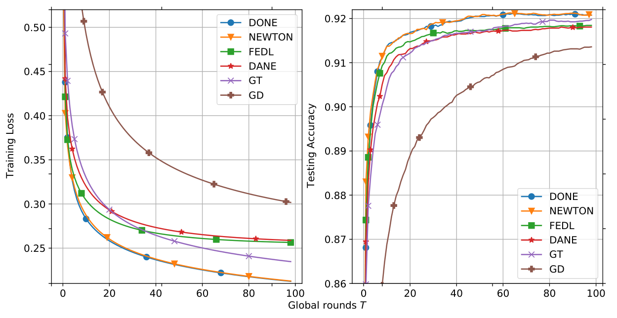
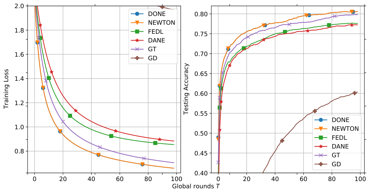
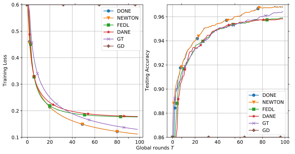
We finally compare DONE with the Newton’s method, GD, DANE, and FEDL. For a fair comparison, we fix a same number of communication rounds ($T$) and the number of local updates ($R$) for all algorithms. We then use grid search to fine-tune the hyper-parameters w.r.t. the highest test accuracy and stability of each algorithm. We fix $\eta=1$ for DANE and choose the best regularization parameter $\mu$ in $\{0,\lambda,3\lambda\}$ for DANE and GIANT ⁷⁷ 7 We direct the reader to [13] for the meaning of DANE’s parameters.. We follow the setting of [14] for FEDL. We also apply the Richardson iteration to the true Newton’s method (3) since it is impractical to do the inverse Hessian. Newton’s method with Richardson iteration requires all edge workers to send the local Newton direction to the server for aggegation at each single local update, hence it actually takes $R.T$ communication rounds. In comparison with Newton’s method, two separate cases are considered: when the Newton’s method has the same values of hyper-parameter $\alpha$ with DONE and uses fine-tuned $\alpha$. We compare the accuracy and running time in Table II and the convergence of all algorithms in Figs. 7(a), 7(b), and 7(c). The experimental results show that DONE has a similar performance to Newton’s method on the same set of $\alpha$ and $R$. As highlighted in Theorem 1, when $\alpha$ is small and $R$ is large enough, the Richardson iteration allows DONE to catch up with the Newton’s method. There is only a small gap (0.12%) when Newton’s method has a larger value of $\alpha$ which can be seen when using the Human Activity, a highly non-i.i.d dataset. To obtain similar performance with Newton’s method in this scenario, DONE needs to run more local iterations ($R=50$). In the case of FEMNIST and MNIST, DONE and the Newton’s method have the same value of fine-tuned $\alpha$. In comparison with others, DONE improves from FEDL, DANE, GAINT, and GD in all real datasets. For MNIST, the improvement in test accuracy compared to FEDL, DANE, GIANT, and GD are approximately 0.22%, 0.27%, 0.22%, and 0.76%, respectively. The corresponding figures are 2.32%, 3.03%, 0.99%, and 20.02% for FEMNIST, and 0.88%, 0.96%, 0.65%, and 16.76% for Human Activity. Finally, to compare the communication and computation complexities among all algorithms, we first fix $T=100$ and compare the running time of all algorithms. The results in Table II show that DONE has the smallest running time. Additionally, in Table III, we set the same target accuracy and compare the number of global rounds $T$ needed by each algorithm to achieve that accuracy. Overall, DONE shows a marked improvement from GIANT, DANE, and FEDL, requiring much fewer iterations to achieve the same accuracy.

By Richardson iteration convergence, it is straightforward to have: $\lim_{k\rightarrow\infty}x_{k}=A^{-1}b=x^{*}$ and

Using the Richardson iteration, expanding $x_{k}$ recursively gives

Similarly, expanding $x_{i,k}$ recursively gives

Taking the average of all $x_{i,k}$ gives

Using the Taylor expansion on $(I-\alpha A)^{j}$ gives

Taking the sum of this term from $j=0$ to $k-1$ gives

For any matrix $A$ and constant $\alpha$ satisfying $\lVert\alpha A_{i}\rVert<1,\forall i$, we can respectively express (15) and (16) as

Substituting (17) and (18) into (12) gives

Similarly, substituting (17) and (18) into (13) gives

If $A=\frac{1}{n}\sum\nolimits_{i=1}^{n}A_{i}$, $\nu=\left\lVert A^{2}-\frac{1}{n}\sum\limits_{i=1}^{n}A_{i}^{2}\right\rVert$, and $x_{0}=x_{i,0}$ we can bound the distance between $x_{k}$ and $\frac{1}{n}\sum\nolimits_{i=1}^{n}x_{i,k}$ as

References

- [1] J. Park, S. Samarakoon, M. Bennis, and M. Debbah, “Wireless Network Intelligence at the Edge,” Proceedings of the IEEE, vol. 107, no. 11, pp. 2204–2239, 2019.
- [2] Z. Zhou et al., “Edge Intelligence: Paving the Last Mile of Artificial Intelligence With Edge Computing,” Proceedings of the IEEE, vol. 107, no. 8, pp. 1738–1762, 2019.
- [3] X. Wang et al., “Convergence of Edge Computing and Deep Learning: A Comprehensive Survey,” IEEE Communications Surveys and Tutorials, vol. 22, no. 2, pp. 869–904, 2020.
- [4] J. Konečný et al., “Federated Learning: Strategies for Improving Communication Efficiency,” arXiv:1610.05492 [cs], Oct. 2017.
- [5] H. B. McMahan, E. Moore, D. Ramage, and S. Hampson, “Communication-Efficient Learning of Deep Networks from Decentralized Data,” in International Conference on Artificial Intelligence and Statistics, 2017.
- [6] J. Konečný, H. B. McMahan, D. Ramage, and P. Richtárik, “Federated Optimization: Distributed Machine Learning for On-Device Intelligence,” arXiv:1610.02527 [cs], Oct. 2016.
- [7] N. H. Tran, W. Bao, A. Zomaya, M. N. H. Nguyen, and C. S. Hong, “Federated Learning over Wireless Networks: Optimization Model Design and Analysis,” in IEEE INFOCOM 2019 - IEEE Conference on Computer Communications, Paris, France, 2019.
- [8] Y. Tu, Y. Ruan, S. Wagle, C. G. Brinton, and C. Joe-Wong, “Network-Aware Optimization of Distributed Learning for Fog Computing,” in IEEE INFOCOM 2020 - IEEE Conference on Computer Communications, Toronto, ON, Canada, 2020.
- [9] J. Wangni, J. Wang, J. Liu, and T. Zhang, “Gradient Sparsification for Communication-Efficient Distributed Optimization,” arXiv:1710.09854 [cs, stat], Oct. 2017.
- [10] L. Bottou, F. E. Curtis, and J. Nocedal, “Optimization Methods for Large-Scale Machine Learning,” SIAM Review, vol. 60, no. 2, pp. 223–311, 2018.
- [11] S. P. Boyd and L. Vandenberghe, Convex Optimization. Cambridge University Press, 2004.
- [12] Y. Nesterov, Introductory Lectures on Convex Optimization: A Basic Course. Springer, 2013.
- [13] O. Shamir, N. Srebro, and T. Zhang, “Communication-efficient distributed optimization using an approximate Newton-Type method,” in 31st International Conference on Machine Learning, Beijing, China, 2014.
- [14] C. T. Dinh et al., “Federated learning over wireless networks: Convergence analysis and resource allocation,” IEEE/ACM Transactions on Networking, vol. 29, no. 1, pp. 398–409, 2021.
- [15] S. Wang, F. Roosta, P. Xu, and M. W. Mahoney, “GIANT: Globally Improved Approximate Newton Method for Distributed Optimization,” in Advances in Neural Information Processing Systems 31, Montréal, Canada, 2018.
- [16] M. Zinkevich, M. Weimer, L. Li, and A. J. Smola, “Parallelized Stochastic Gradient Descent,” in Advances in Neural Information Processing Systems 23, Vancouver, BC, Canada, 2010.
- [17] O. Shamir and N. Srebro, “Distributed stochastic optimization and learning,” in 52nd Annual Allerton Conference on Communication, Control, and Computing, Monticello, IL, USA, 2014.
- [18] J. D. Lee, Q. Lin, T. Ma, and T. Yang, “Distributed Stochastic Variance Reduced Gradient Methods by Sampling Extra Data with Replacement,” Journal of Machine Learning Research, vol. 18, no. 122, pp. 1–43, 2017.
- [19] S. J. Reddi, J. Konečný, P. Richtárik, B. Póczós, and A. Smola, “AIDE: Fast and Communication Efficient Distributed Optimization.” arXiv: 1608.06879, 2016.
- [20] P. Richtárik and M. Takáč, “Distributed coordinate descent method for learning with big data,” Journal of Machine Learning Research, vol. 17, no. 1, pp. 2657–2681, 2016.
- [21] T. Yang, “Trading Computation for Communication: Distributed Stochastic Dual Coordinate Ascent,” in Advances in Neural Information Processing Systems 26, Lake Tahoe, Nevada, USA, 2013.
- [22] W. Shi, S. Zhou, and Z. Niu, “Device Scheduling with Fast Convergence for Wireless Federated Learning,” arXiv:1911.00856 [cs, math], Nov. 2019.
- [23] H. H. Yang, Z. Liu, T. Q. S. Quek, and H. V. Poor, “Scheduling Policies for Federated Learning in Wireless Networks,” IEEE Transactions on Communications, vol. 68, no. 1, pp. 317–333, Jan. 2020.
- [24] H. Tang, C. Yu, X. Lian, T. Zhang, and J. Liu, “DoubleSqueeze: Parallel Stochastic Gradient Descent with Double-pass Error-Compensated Compression,” in Proceedings of the 36th International Conference on Machine Learning. PMLR, May 2019, pp. 6155–6165.
- [25] Y. Zhang and L. Xiao, “DiSCO: Distributed optimization for self-concordant empirical loss,” in 32nd International Conference on Machine Learning, Lille, France, 2015.
- [26] S. Wang et al., “Adaptive Federated Learning in Resource Constrained Edge Computing Systems,” IEEE Journal on Selected Areas in Communications, vol. 37, no. 6, pp. 1205–1221, 2019.
- [27] W. C. Rheinboldt, “Classical Iterative Methods for Linear Systems,” 2009.
- [28] T. Hastie, R. Tibshirani, and J. H. Friedman, The Elements of Statistical Learning: Data Mining, Inference, and Prediction, 2nd ed. Springer, 2009.
- [29] B. Polyak and A. Tremba, “New versions of Newton method: Step-size choice, convergence domain and under-Determined equations,” Optimization Methods and Software, vol. 35, no. 6, pp. 1272–1303, Nov. 2020.
- [30] M. Li et al., “Scaling distributed machine learning with the parameter server,” in 11th USENIX Conference on Operating Systems Design and Implementation, Broomfield, CO, USA, 2014.
- [31] M. Li, D. G. Andersen, A. J. Smola, and K. Yu, “Communication Efficient Distributed Machine Learning with the Parameter Server,” in Advances in Neural Information Processing Systems 27, Montreal, Quebec, Canada, 2014.
- [32] S. U. Stich, “Local SGD Converges Fast and Communicates Little,” in 7th International Conference on Learning Representations, New Orleans, LA, USA, 2018.
- [33] Y. Lecun, L. Bottou, Y. Bengio, and P. Haffner, “Gradient-based learning applied to document recognition,” Proceedings of the IEEE, vol. 86, no. 11, pp. 2278–2324, 1998.
- [34] G. Cohen, S. Afshar, J. Tapson, and A. van Schaik, “EMNIST: Extending MNIST to handwritten letters,” in International Joint Conference on Neural Networks, 2017.
- [35] T. Li et al., “Federated Optimization in Heterogeneous Networks,” in Proceedings of the 3rd MLSys Conference, Austin, TX, USA, 2020.
- [36] D. Anguita, A. Ghio, L. Oneto, X. Parra, and J. L. Reyes-Ortiz, “A Public Domain Dataset for Human Activity Recognition Using Smartphones,” in European Symposium on Artificial Neural Networks, Computational Intelligence and Machine Learning, 2013.
![[Uncaptioned image]](2012.05625v4/authors/1_Dinh.jpg) |
Canh T. Dinh received the BE degree in Electronics and Telecommunication from Ha Noi University of Science and Technology, Ha Noi City, Vietnam, in 2015 and Master of Data Science degree from Université Grenoble Alpes, Grenoble, France, in 2019. He is currently pursuing a Ph.D. degree in Computer Science at The University of Sydney, Sydney, Australia. His supervisor is Dr. Nguyen H. Tran. His research interests include Federated Learning and privacy machine learning. |
![[Uncaptioned image]](2012.05625v4/authors/2_Tran.jpg) |
Nguyen H. Tran (S’10-M’11-SM’18) received BS and Ph.D degrees, from HCMC University of Technology and Kyung Hee University, in electrical and computer engineering, in 2005 and 2011, respectively. He was an Assistant Professor with Department of Computer Science and Engineering, Kyung Hee University, from 2012 to 2017. Since 2018, he has been with the School of Computer Science, The University of Sydney, where he is currently a Senior Lecturer. His research interests include distributed computing, machine learning, and networking. He received the best KHU thesis award in engineering in 2011 and several best paper awards, including IEEE ICC 2016 and ACM MSWiM 2019. He receives the Korea NRF Funding for Basic Science and Research 2016-2023 and ARC Discovery Project 2020-2023. He was the Editor of IEEE Transactions on Green Communications and Networking from 2016 to 2020, and the Associate Editor of IEEE Journal of Selected Areas in Communications 2020 in the area of distributed machine learning/Federated Learning. |
![[Uncaptioned image]](2012.05625v4/authors/3_Nguyen.jpg) |
Tuan Dung Nguyen received a B.S. in computer science from the University of Melbourne, Australia. He is currently an M.Phil. candidate at the Computational Media Lab, the Australian National University. His research interests include distributed optimization, machine learning and computational social science. |
![[Uncaptioned image]](2012.05625v4/authors/5_WeiBao.jpg) |
Wei Bao (S’10-M’16) received the B.E. degree in Communications Engineering from the Beijing University of Posts and Telecommunications, Beijing, China, in 2009; the M.A.Sc. degree in Electrical and Computer Engineering from the University of British Columbia, Vancouver, Canada, in 2011; and the PhD degree in Electrical and Computer Engineering from the University of Toronto, Toronto, Canada, in 2016. He is currently a senior lecturer at the School of Computer Science, the University of Sydney, Sydney, Australia. His research covers the area of network science, with particular emphasis on Internet of things, mobile computing, and edge computing. He received the Best Paper Awards in ACM International Conference on Modeling, Analysis and Simulation of Wireless and Mobile Systems (MSWiM) in 2013 and 2019 and IEEE International Symposium on Network Computing and Applications (NCA) in 2016. |
![[Uncaptioned image]](2012.05625v4/authors/8_Amir.jpg) |
Amir R. Balef received the BE degree in Electrical Engineering from Amirkabir University of Technology, Tehran, Iran, in 2017 and M.Sc. degree ,in field of Digital systems, from Sharif University of Technology, Tehran, Iran in 2019. His research interests include edge computing, Internet of Things, privacy-preserving machine learning, federated learning. In recent years, he has focused on optimization algorithms. |
![[Uncaptioned image]](2012.05625v4/authors/BingBingZhou.jpg) |
Bing Bing Zhou received the graduate degree in electronic engineering, in 1982 from the Nanjing Institute of Technology in China, and the PhD degree in computer science, in 1989 from Australian National University, Australia. He is an associate professor in the School of Computer Science, the University of Sydney, Australia (2003-present). Currently, he is the theme leader for distributed computing applications in the Centre for Distributed and High Performance Computing at the University of Sydney. |
![[Uncaptioned image]](2012.05625v4/authors/6_Albert.jpg) |
Albert Y. ZOMAYA is Chair Professor of High-Performance Computing and Networking in the School of Computer Science and Director of the Centre for Distributed and High-Performance Computing at the University of Sydney. To date, he has published more than 600 scientific papers and articles and is (co-)author/editor of more than 30 books. A sought-after speaker, he has delivered more than 190 keynote addresses, invited seminars, and media briefings. His research interests span several areas in parallel and distributed computing and complex systems. He is currently the Editor in Chief of the ACM Computing Surveys and served in the past as Editor in Chief of the IEEE Transactions on Computers (2010-2014) and the IEEE Transactions on Sustainable Computing (2016-2020). Professor Zomaya is a decorated scholar with numerous accolades including Fellowship of the IEEE, the American Association for the Advancement of Science, and the Institution of Engineering and Technology (UK). Also, he is an Elected Fellow of the Royal Society of New South Wales and an Elected Foreign Member of Academia Europaea. He is the recipient of the 1997 Edgeworth David Medal from the Royal Society of New South Wales for outstanding contributions to Australian Science, the IEEE Technical Committee on Parallel Processing Outstanding Service Award (2011), IEEE Technical Committee on Scalable Computing Medal for Excellence in Scalable Computing (2011), IEEE Computer Society Technical Achievement Award (2014), ACM MSWIM Reginald A. Fessenden Award (2017), and the New South Wales Premier’s Prize of Excellence in Engineering and Information and Communications Technology (2019). |