跳到论文正文
W Papers独立论文阅读器 arXiv:2012.05602 论文正文 计算阅读时间 · 0%
引用这篇论文根据当前论文元数据生成,正式投稿前建议核对。


License: arXiv.org perpetual non-exclusive license
arXiv:2012.05602v2 [math.PR] 07 Jul 2021

Convergence of the spectral radius of a random matrix
through its characteristic polynomialThanks: CB and DGZ are supported by the grant ANR-16-CE40-0024

Charles Bordenave Address: Institut de Mathématiques de Marseille; CNRS; Aix-Marseille Université, Marseille, France. Email address: charles.bordenave@univ-amu.fr URL: http://www.i2m.univ-amu.fr/perso/charles.bordenave/ , Djalil Chafaï Address: CEREMADE, CNRS, UMR 7534, Université Paris-Dauphine, PSL University, 75016 Paris, France. Email address: djalil@chafai.net URL: http://djalil.chafai.net/ and David García-Zelada Address: Institut de Mathématiques de Marseille; CNRS; Aix-Marseille Université, Marseille, France. Email address: david.garcia-zelada@univ-amu.fr URL: https://davidgarciaz.wixsite.com/math
Date: Autumn 2020, revised Summer 2021. Preprint, compiled August 11, 2026.
Abstract.

Consider a square random matrix with independent and identically distributed entries of mean zero and unit variance. We show that as the dimension tends to infinity, the spectral radius is equivalent to the square root of the dimension in probability. This result can also be seen as the convergence of the support in the circular law theorem under optimal moment conditions. In the proof we establish the convergence in law of the reciprocal characteristic polynomial to a random analytic function outside the unit disc, related to a hyperbolic Gaussian analytic function. The proof is short and differs from the usual approaches for the spectral radius. It relies on a tightness argument and a joint central limit phenomenon for traces of fixed powers.

Key words and phrases:
Random Matrix; Spectral Radius; Gaussian Analytic Function; Central Limit Theorem; Combinatorics; Digraph; Circular Law
2010 Mathematics Subject Classification
Primary: 30C15, 60B20; Secondary: 60F05

1. Introduction and main results

Let {aj​k}j,k≥1\{a_{jk}\}_{j,k\geq 1} be independent and identically distributed complex random variables with mean zero and unit variance, namely 𝔼⁡[a11]=0\mathbb{E}[a_{11}]=0 and 𝔼⁡[|a11|2]=1\mathbb{E}[|a_{11}|^{2}]=1. For all n≥1n\geq 1, let

(1.1) An=(aj​k)1≤j,k≤n.A_{n}={(a_{jk})}_{1\leq j,k\leq n}.

We call it a Girko matrix [13]. When a11a_{11} is Gaussian with independent and identically distributed real and imaginary parts then AnA_{n} has density proportional to e−Tr⁡(A​A∗)\mathrm{e}^{-\mathrm{Tr}(AA^{*})} and belongs to the complex Ginibre ensemble [11]. We are interested in the matrix 1n​An\frac{1}{\sqrt{n}}A_{n} for which each row and each column has a unit mean squared Euclidean norm. Its characteristic polynomial at point z∈ℂz\in\mathbb{C} is

(1.2) pn(z)=det(z−Ann)p_{n}(z)=\det\Bigr(z-\frac{A_{n}}{\sqrt{n}}\Bigr)

where zz stands for zz times the identity matrix. The nn roots of pnp_{n} in ℂ\mathbb{C} are the eigenvalues of 1n​An\frac{1}{\sqrt{n}}A_{n}. They form a multiset Λn\Lambda_{n} which is the spectrum of 1n​An\frac{1}{\sqrt{n}}A_{n}. The spectral radius of 1n​An\frac{1}{\sqrt{n}}A_{n} is defined by

(1.3) ρn=maxλ∈Λn⁡|λ|.\rho_{n}=\max_{\lambda\in\Lambda_{n}}|\lambda|.

The circular law theorem states that the empirical measure of the elements of Λn\Lambda_{n} tends weakly as n→∞n\to\infty to the uniform distribution on the closed unit disc: almost surely, for every nice Borel set B⊂ℂB\subset\mathbb{C},

(1.4) limn→∞card⁡(B∩Λn)n=area⁡(B∩𝔻¯)π,\lim_{n\to\infty}\frac{\mathrm{card}(B\cap\Lambda_{n})}{n}=\frac{\mathrm{area}(B\cap\overline{\mathbb{D}})}{\pi},

where “area\mathrm{area}” stands for the Lebesgue measure on ℂ\mathbb{C}, and where 𝔻¯={z∈ℂ:|z|≤1}\overline{\mathbb{D}}=\{z\in\mathbb{C}:|z|\leq 1\} is the closed unit disc, see [12, 13, 21, 6]. The circular law (1.4), which involves weak convergence, does not provide the convergence of the spectral radius, it gives only that almost surely

(1.5) lim¯n→∞⁡ρn≥1.\varliminf_{n\to\infty}\rho_{n}\geq 1.

Theorem 1.1 provides the convergence of the spectral radius, without extra assumptions on the entries. This result was conjectured in [5], and improves over [10, 16, 1, 5, 3]. The moments assumptions are optimal, and the 1n\frac{1}{\sqrt{n}} scaling is no longer adequate for entries of infinite variance, see for instance [4].

We have ρn≤σn\rho_{n}\leq\sigma_{n} where σn\sigma_{n} is the operator norm of 1n​An\frac{1}{\sqrt{n}}A_{n}, its largest singular value. It is known that the condition 𝔼⁡[|a11|4]<∞\mathbb{E}[|a_{11}|^{4}]<\infty is necessary and sufficient for the convergence of σn\sigma_{n} as n→∞n\to\infty, see [2]. A stricking aspect of the spectral radius is that it converges without any extra moment condition.

Theorem 1.1 (Spectral radius).

We have limn→∞ρn=1\lim_{n\to\infty}\rho_{n}=1 in probability, in the sense that for all ε>0\varepsilon>0,

limn→∞ℙ⁡(|ρn−1|≥ε)=0.\lim_{n\to\infty}\mathbb{P}(|\rho_{n}-1|\geq\varepsilon)=0.

The proof of Theorem 1.1 is given in Section 2. It relies on Theorem 1.2 below, which is of independent interest. It does not involve any Hermitization or norms of powers in the spirit of Gelfand’s spectral radius formula. The idea is to show that on ℂ∪{∞}∖𝔻¯\mathbb{C}\cup\{\infty\}\setminus\overline{\mathbb{D}}, the polynomial z−n​pn​(z)z^{-n}p_{n}(z) tends as n→∞n\to\infty to a random analytic function which does not vanish. The first step for mathematical convenience is to convert ℂ∪{∞}∖𝔻¯\mathbb{C}\cup\{\infty\}\setminus\overline{\mathbb{D}} into 𝔻={z∈ℂ:|z|<1}\mathbb{D}=\{z\in\mathbb{C}:|z|<1\} by noting that pn​(z)=zn​qn​(1/z)p_{n}(z)=z^{n}q_{n}(1/z), z∉𝔻¯z\not\in\overline{\mathbb{D}}, where for all z∈𝔻z\in\mathbb{D},

qn​(z)=det(1−z​Ann)q_{n}(z)=\det\left(1-z\frac{A_{n}}{\sqrt{n}}\right)

is the reciprocal polynomial of the characteristic polynomial pnp_{n}. Let H⁡(𝔻)\mathrm{H}(\mathbb{D}) be the set of holomorphic or complex analytic functions on 𝔻\mathbb{D}, equipped with the topology of uniform convergence on compact subsets, the compact-open topology, see for instance [20]. This allows to see qnq_{n} as a random variable on H⁡(𝔻)\mathrm{H}(\mathbb{D}) and gives a meaning to convergence in law of qnq_{n} as n→∞n\to\infty, namely, qnq_{n} converges in law to some random element qq of H⁡(𝔻)\mathrm{H}(\mathbb{D}) if for every bounded real continuous function ff on H⁡(𝔻)\mathrm{H}(\mathbb{D}), 𝔼⁡[f⁡(qn)]→𝔼⁡[f⁡(q)]\mathbb{E}[f(q_{n})]\to\mathbb{E}[f(q)].

Theorem 1.2 (Convergence of reciprocal characteristic polynomial).

We have

qn→n→∞lawκ​e−F,q_{n}\xrightarrow[n\to\infty]{\mathrm{law}}\kappa\mathrm{e}^{-F},

where FF is the random holomorphic function on 𝔻\mathbb{D} defined by

F⁡(z)=∑k=1∞Xk​zkkF(z)=\sum_{k=1}^{\infty}X_{k}\frac{z^{k}}{\sqrt{k}}

where {Xk}k≥1\{X_{k}\}_{k\geq 1} is a sequence of independent complex Gaussian random variables such that

𝔼[Xk]=0,𝔼[|Xk|2]=1and𝔼[Xk2]=𝔼[a112]k,\mathbb{E}\big[X_{k}\big]=0,\quad\mathbb{E}\left[|X_{k}|^{2}\right]=1\quad\text{and}\quad\mathbb{E}\left[X_{k}^{2}\right]=\mathbb{E}\left[a_{11}^{2}\right]^{k},

and where κ:𝔻→ℂ\kappa:\mathbb{D}\to\mathbb{C} is the holomorphic function defined for all z∈𝔻z\in\mathbb{D} by

κ⁡(z)=1−z2​𝔼​[a112].\kappa(z)=\sqrt{1-z^{2}\mathbb{E}\left[a_{11}^{2}\right]}.

The square root defining κ\kappa is the one such that κ⁡(0)=1\kappa(0)=1. Notice that it is a well-defined holomorphic function on the simply connected domain 𝔻\mathbb{D} since the function z↦1−z2​𝔼​[a112]z\mapsto 1-z^{2}\mathbb{E}[a_{11}^{2}] does not vanish on 𝔻\mathbb{D} which is true due to the fact that |𝔼⁡[a112]|≤𝔼⁡[|a11|2]=1|\mathbb{E}[a_{11}^{2}]|\leq\mathbb{E}[|a_{11}|^{2}]=1.

The proof of Theorem 1.2 is given in Section 3. It is partially inspired by [3] and relies crucially on a joint combinatorial central limit theorem for traces of fixed powers (Lemma 3.4) inspired from [17]. Unlike previous arguments used in the literature for the analysis of Girko matrices, the approach does not rely on Girko Hermitization, Gelfand spectral radius formula, high order traces, resolvent method or Cauchy – Stieltjes transform. The first step consists in showing the tightness of (qn)n≥1{(q_{n})}_{n\geq 1}, by using a decomposition of the determinant into orthogonal elements related to determinants of submatrices, as in [3]. Knowing this tightness, the problem is reduced to show the convergence in law of these elements. A reduction step, inspired by [17], consists in truncating the entries, reducing the analysis to the case of bounded entries. The next step consists in a central limit theorem for product of traces of powers of fixed order. It is important to note that we truncate with a fixed threshold with respect to nn, and the order of the powers in the traces are fixed with respect to nn. This is in sharp contrast with the usual Füredi – Komlós truncation-trace approach related to the Gelfand spectral radius formula used in [10, 16, 1, 5].

1.1. Comments and open problems

1.1.1. Moment assumptions.

The universality for the first order global asymptotics (1.4) depends only on the trace 𝔼⁡[|a11|2]\mathbb{E}[|a_{11}|^{2}] of the covariance matrix of ℜ⁡a11\Re a_{11} and ℑ⁡a11\Im a_{11}. The universality stated by Theorem 1.2, just like for the central limit theorem, depends on the whole covariance matrix. Since

𝔼⁡[a112]=𝔼⁡[(ℜ⁡a11)2]−𝔼⁡[(ℑ⁡a11)2]+2​i​𝔼​[ℜ⁡a11​ℑ​a11],\mathbb{E}[a_{11}^{2}]=\mathbb{E}[(\Re a_{11})^{2}]-\mathbb{E}[(\Im a_{11})^{2}]+2\mathrm{i}\mathbb{E}[\Re a_{11}\Im a_{11}],

we can see that 𝔼⁡[a112]=0\mathbb{E}[a_{11}^{2}]=0 if and only if 𝔼⁡[(ℜ⁡a11)2]=𝔼⁡[(ℑ⁡a11)2]\mathbb{E}[(\Re a_{11})^{2}]=\mathbb{E}[(\Im a_{11})^{2}] and 𝔼⁡[ℜ⁡a11​ℑ⁡a11]=0\mathbb{E}[\Re a_{11}\Im a_{11}]=0. Moreover, we cannot in general get rid of 𝔼⁡[a112]\mathbb{E}[a_{11}^{2}] by simply multiplying the matrix AnA_{n} by a phase.

1.1.2. Hyperbolic Gaussian analytic function

When 𝔼⁡[a112]=0\mathbb{E}\left[a_{11}^{2}\right]=0 then κ=1\kappa=1 while the random analytic function FF which appears in the limit in Theorem 3 is a degenerate case of the well-known hyperbolic Gaussian Analytic Functions (GAFs) [14, Equation (2.3.5)]. It can also be obtained as the antiderivative of the L=2L=2 hyperbolic GAF which is 00 at z=0z=0. This L=2L=2 hyperbolic GAF is related to the Bergman kernel and could be called the Bergman GAF. These GAFs appear also at various places in mathematics and physics and, in particular, in the asymptotic analysis of Haar unitary matrices, see [15, 18].

1.1.3. Cauchy – Stieltjes transform

If 𝔼⁡[a112]=0\mathbb{E}[a_{11}^{2}]=0 then by returning to pnp_{n}, taking the logarithm and the derivative with respect to zz in Theorem 1.2, we obtain the convergence in law of the Cauchy – Stieltjes transform (complex conjugate of the electric field) minus n/zn/z towards z↦F′​(1/z)/z2z\mapsto F^{\prime}(1/z)/z^{2} which is a Gaussian analytic function on ℂ∖𝔻¯\mathbb{C}\setminus\overline{\mathbb{D}} with covariance given by a Bergman kernel.

1.1.4. Central Limit Theorem

We should see Theorem 1.2 as a global second order analysis, just like the central limit theorem (CLT) for linear spectral statistics [19, 9, 8]. Namely for all z∈𝔻z\in\mathbb{D}, we have |qn​(1/z)|=exp⁡[−n⁡(Un​(z)−U⁡(z))]|q_{n}(1/z)|=\exp\left[-n\left(U_{n}(z)-U(z)\right)\right] where Un​(z)=−1n​log⁡|pn​(z)|U_{n}(z)=-\frac{1}{n}\log|p_{n}(z)| is the logarithmic potential at the point zz of the empirical spectral distribution of 1n​An\frac{1}{\sqrt{n}}A_{n} and U⁡(z)=−log⁡|z|U(z)=-\log|z| is the logarithmic potential at the point zz of the uniform distribution on the unit disc 𝔻\mathbb{D}.

Moreover, it is possible to extract from Theorem 1.2 a CLT for linear spectral statistics with respect to analytic functions in a neighborhood of 𝔻¯\overline{\mathbb{D}}. This can be done by using the Cauchy formula for an analytic function ff,

∫f(λ)μ(dλ)=12​π​i∫(∮f⁡(z)z−λdz)μ(dλ)=12​π​i∮f(z)(∫μ⁡(d​λ)z−λ)dz=12​π​i∮f(z)(logdet(z−A))′dz\int f(\lambda)\mathrm{\mu}(\mathrm{d}\lambda)=\frac{1}{2\pi\mathrm{i}}\int\left(\oint\frac{f(z)}{z-\lambda}\mathrm{d}z\right)\mu(\mathrm{d}\lambda)=\frac{1}{2\pi\mathrm{i}}\oint f(z)\left(\int\frac{\mu(\mathrm{d}\lambda)}{z-\lambda}\right)\mathrm{d}z\\ =\frac{1}{2\pi\mathrm{i}}\oint f(z)(\log\det\left(z-A\right))^{\prime}\mathrm{d}z

where μ\mu is the counting measure of the eigenvalues of AA, where the contour integral is around a centered circle of radius strictly larger than 11, and where we have taken any branch of the logarithm. The approach is purely complex analytic. In particular, it is different from the usual approach with the logarithmic potential of μ\mu based on the real function given by z↦∫log⁡|z−λ|​μ​(𝑑λ)=log⁡|det(z−A)|z\mapsto\int\log|z-\lambda|\mu(\mathrm{d}\lambda)=\log|\det(z-A)|.

1.1.5. Wigner case and elliptic interpolation

The finite second moment assumption of Theorem 1.1 is optimal. We could explore its relation with the finite fourth moment assumption for the convergence of the spectral edge of Wigner random matrices, which is also optimal. Heuristic arguments tell us that the interpolating condition on the matrix entries should be 𝔼⁡[|aj​k|2​|ak​j|2]<∞\mathbb{E}[|a_{jk}|^{2}|a_{kj}|^{2}]<\infty for j≠kj\neq k, which is a finite second moment condition for Girko matrices and a finite fourth moment condition for Wigner matrices. This is work in progress.

1.1.6. Coupling and almost sure convergence

For simplicity, we define in (1.1) our random matrix AnA_{n} for all n≥1n\geq 1 by truncating from the upper left corner the infinite random matrix {aj​k}j,k≥1\{a_{jk}\}_{j,k\geq 1}. This imposes a coupling for the matrices {An}n≥1\{A_{n}\}_{n\geq 1}. However, since Theorem 1.1 involves a convergence in probability, it remains valid for an arbitrary coupling, in the spirit of the triangular arrays assumptions used for classical central limit theorems. In another direction, one could ask about the upgrade of the convergence in probability into almost sure convergence in Theorem 1.1. This is an open problem.

1.1.7. Heavy tails

An analogue of (1.4) in the heavy-tailed case 𝔼⁡[|a11|2]=∞\mathbb{E}[|a_{11}|^{2}]=\infty is considered in [4] but requires another scaling than 1n\frac{1}{\sqrt{n}}. The spectral radius of this model tends to infinity as n→∞n\to\infty but it could be possible to analyze the limiting point process at the edge as n→∞n\to\infty and its universality. This is an open problem.

2. Proof of Theorem 1.1

Let f=κ​e−Ff=\kappa\mathrm{e}^{-F} be as in Theorem 1.2. We observe that the equation f⁡(z)=0f(z)=0, z∈𝔻z\in\mathbb{D} is equivalent to κ⁡(z)=0\kappa(z)=0, z∈𝔻z\in\mathbb{D}, which has no solution, because |𝔼⁡[a112]|≤𝔼⁡[|a11|2]=1|\mathbb{E}[a_{11}^{2}]|\leq\mathbb{E}[|a_{11}|^{2}]=1. In particular, for every r∈(0,1)r\in(0,1),

infz∈D¯r|f⁡(z)|=infz∈D¯r{|κ⁡(z)|​e−ℜ⁡(F⁡(z))}>0,\inf_{z\in\overline{D}_{r}}|f(z)|=\inf_{z\in\overline{D}_{r}}\left\{|\kappa(z)|\mathrm{e}^{-\Re(F(z))}\right\}>0,

where D¯r={z∈ℂ:|z|≤r}\overline{D}_{r}=\{z\in\mathbb{C}:|z|\leq r\} is the closed disc of radius rr. On the other hand, the convergence in law provided by Theorem 1.2 together with the continuous mapping theorem used for the continuous function f∈H⁡(𝔻)↦infz∈D¯r|f⁡(z)|f\in\mathrm{H}(\mathbb{D})\mapsto\inf_{z\in\overline{D}_{r}}|f(z)| give, for every r∈(0,1)r\in(0,1),

infz∈D¯r|qn​(z)|→n→∞lawinfz∈D¯r{|κ⁡(z)|​e−ℜ⁡(F⁡(z))}.\inf_{z\in\overline{D}_{r}}|q_{n}(z)|\xrightarrow[n\to\infty]{\mathrm{law}}\inf_{z\in\overline{D}_{r}}\left\{|\kappa(z)|\mathrm{e}^{-\Re(F(z))}\right\}.

Now, since qn​(z)=zn​pn​(1/z)q_{n}(z)=z^{n}p_{n}(1/z) for every z∈𝔻z\in\mathbb{D}, we obtain, by combining these two facts, for every r∈(0,1)r\in(0,1),

ℙ(ρn<1r)=ℙ(inf|z|≥1r|pn(z)|>0)=ℙ(infz∈D¯r|qn(z)|>0)→n→∞ℙ(infz∈D¯r{|κ(z)|e−ℜ⁡(F⁡(z))}>0)=1.\mathbb{P}\Bigr(\rho_{n}<\frac{1}{r}\Bigr)=\mathbb{P}\Bigr(\inf_{|z|\geq\frac{1}{r}}|p_{n}(z)|>0\Bigr)=\mathbb{P}\Bigr(\inf_{z\in\overline{D}_{r}}|q_{n}(z)|>0\Bigr)\xrightarrow[n\to\infty]{}\mathbb{P}\Bigr(\inf_{z\in\overline{D}_{r}}\left\{|\kappa(z)|\mathrm{e}^{-\Re(F(z))}\right\}>0\Bigr)=1.

In other words, for all ε>0\varepsilon>0,

limn→∞ℙ⁡(ρn≥1+ε)=0.\lim_{n\to\infty}\mathbb{P}(\rho_{n}\geq 1+\varepsilon)=0.

Combined with (1.5), this leads to the desired result

limn→∞ℙ⁡(|ρn−1|>ε)=0.\lim_{n\to\infty}\mathbb{P}(|\rho_{n}-1|>\varepsilon)=0.

Note that it could be possible to obtain the result by using the Radon measures of the zeros and the Hurwitz phenomenon, see [20, Lemma 2.2] and [7, Lemma 5.2], but this would be more complicated!

3. Proof of Theorem 1.2

By developing the determinant we can see that

qn​(z)=det(1−z​Ann)=1+∑k=1n(−z)k​Pk(n),q_{n}(z)=\det\left(1-z\frac{A_{n}}{\sqrt{n}}\right)=1+\sum_{k=1}^{n}(-z)^{k}P^{(n)}_{k},

where

Pk(n)=∑I⊂{1,…,n}|I|=kn−k/2det(An(I))andAn(I)={aj​k}j,k∈I.P^{(n)}_{k}=\sum_{\begin{subarray}{c}I\subset\{1,\dots,n\}\\ |I|=k\end{subarray}}n^{-k/2}\det(A_{n}(I))\quad\text{and}\quad A_{n}(I)=\{a_{jk}\}_{j,k\in I}.

The following lemma is essentially contained in [3, Appendix A]. It is proved in Section 4.1.

Lemma 3.1 (Tightness).

The sequence {qn}n≥1\{q_{n}\}_{n\geq 1} is tight.

For completeness, let us recall that the sequence {qn}n≥1\{q_{n}\}_{n\geq 1} is tight if for every ε>0\varepsilon>0, there exists a compact subset of H⁡(𝔻)\mathrm{H}(\mathbb{D}) such that ℙ⁡(qn∈K)>1−ε\mathbb{P}(q_{n}\in K)>1-\varepsilon for every nn.

Now that we know that {qn}n≥1\{q_{n}\}_{n\geq 1} is tight, it is enough to understand, for each k≥1k\geq 1, the limit of (P1(n),…,Pk(n))(P_{1}^{(n)},\dots,P_{k}^{(n)}) as n→∞n\to\infty. Indeed, we have the following Lemma 3.2, close to [20, Second part of Proposition 2.5]. For the reader’s convenience and for completeness, we give a proof in Section 4.2.

Lemma 3.2 (Reduction to convergence of coefficients).

Let {fn}n≥1\{f_{n}\}_{n\geq 1} be a tight sequence of random elements of H⁡(𝔻)\mathrm{H}(\mathbb{D}), and let us write, for every n≥1n\geq 1, fn​(z)=∑k=0∞zk​Pk(n)f_{n}(z)=\sum_{k=0}^{\infty}z^{k}P_{k}^{(n)}. If for every m≥0m\geq 0,

(P0(n),…,Pm(n))→n→∞law(P0,…,Pm)(P_{0}^{(n)},\dots,P_{m}^{(n)})\xrightarrow[n\to\infty]{\mathrm{law}}(P_{0},\dots,P_{m})

for a common sequence of random variables {Pm}m≥0\{P_{m}\}_{m\geq 0} then f=∑k=0∞zk​Pkf=\sum_{k=0}^{\infty}z^{k}P_{k} is well-defined in H⁡(𝔻)\mathrm{H}(\mathbb{D}) and

fn→n→∞lawf.f_{n}\xrightarrow[n\to\infty]{\mathrm{law}}f.

The first simplification we shall make is to assume that a11a_{11} is bounded. This is motivated by [17, Proof of Lemma 7]. We write this in the following lemma, proved in Section 4.3.

Lemma 3.3 (Reduction to bounded entries by truncation).

For M>0M>0 let us define

An(M)={ai​j(M)}1≤i,j≤nwhereai​j(M)=ai​j​1|ai​j|<M−𝔼⁡[ai​j​1|ai​j|<M]A_{n}^{(M)}=\left\{a_{ij}^{(M)}\right\}_{1\leq i,j\leq n}\quad\text{where}\quad a_{ij}^{(M)}=a_{ij}1_{|a_{ij}|<M}-\mathbb{E}\left[a_{ij}1_{|a_{ij}|<M}\right]

and

Pk(n,M)=∑I⊂{1,…,n}|I|=kn−k/2det(An(M)(I))whereAn(M)(I)={ai​j(M)}i,j∈I.P^{(n,M)}_{k}=\sum_{\begin{subarray}{c}I\subset\{1,\dots,n\}\\ |I|=k\end{subarray}}n^{-k/2}\det(A_{n}^{(M)}(I))\quad\text{where}\quad A_{n}^{(M)}(I)=\left\{a_{ij}^{(M)}\right\}_{i,j\in I}.

Let k≥1k\geq 1. If there exists {(Y1(M),…,Yk(M))}M≥1\left\{\left(Y_{1}^{(M)},\dots,Y_{k}^{(M)}\right)\right\}_{M\geq 1} and a random vector (Y1,…,Yk)\left(Y_{1},\dots,Y_{k}\right) such that for all M≥1M\geq 1,

(P1(n,M),…,Pk(n,M))→n→∞law(Y1(M),…,Yk(M)),and(Y1(M),…,Yk(M))→M→∞law(Y1,…,Yk),\left(P_{1}^{(n,M)},\dots,P_{k}^{(n,M)}\right)\xrightarrow[n\to\infty]{\mathrm{law}}\left(Y_{1}^{(M)},\dots,Y_{k}^{(M)}\right),\quad\text{and}\quad\left(Y_{1}^{(M)},\dots,Y_{k}^{(M)}\right)\xrightarrow[M\to\infty]{\mathrm{law}}\Big(Y_{1},\dots,Y_{k}\Big),

then

(P1(n),…,Pk(n))→n→∞law(Y1,…,Yk).(P_{1}^{(n)},\dots,P_{k}^{(n)})\xrightarrow[n\to\infty]{\mathrm{law}}(Y_{1},\dots,Y_{k}).

To simplify the study of Pk(n)P_{k}^{(n)} we notice the following. For each integer n≥1n\geq 1, the series

Bn=−∑k=1∞(Ann)kzkkB_{n}=-\sum_{k=1}^{\infty}\left(\frac{A_{n}}{\sqrt{n}}\right)^{k}\frac{z^{k}}{k}

converges for zz small enough and its exponential is (1−z​Ann)\left(1-z\frac{A_{n}}{\sqrt{n}}\right). This can be shown in the standard way if AnA_{n} is diagonalizable and can be extended to non-diagonalizable matrices by continuity. Then, since det(eBn)=eTr​Bn\det\left(\mathrm{e}^{B_{n}}\right)=\mathrm{e}^{\mathrm{Tr}B_{n}}, we obtain

qn(z)=exp(−∑k=1∞Tr⁡(Ank)nk/2zkk)q_{n}(z)=\exp\left(-\sum_{k=1}^{\infty}\frac{\mathrm{Tr}(A_{n}^{k})}{n^{k/2}}\frac{z^{k}}{k}\right)

for zz small enough. In particular, (P1(n),…,Pk(n))(P_{1}^{(n)},\dots,P_{k}^{(n)}) is a polynomial function of (Tr⁡(An)n1/2,…,Tr⁡(Ank)nk/2)\left(\frac{\mathrm{Tr}(A_{n})}{n^{1/2}},\dots,\frac{\mathrm{Tr}(A_{n}^{k})}{n^{k/2}}\right) that does not depend on nn and vice versa. The idea is to study, by the method of moments, the quantity

Tr⁡(Ank)=∑1≤i1,…,ik≤nai1​i2​ai2​i3​…​aik−1​ik​aik​i1.\mathrm{Tr}(A_{n}^{k})=\sum_{1\leq i_{1},\dots,i_{k}\leq n}a_{i_{1}i_{2}}a_{i_{2}i_{3}}\dots a_{i_{k-1}i_{k}}a_{i_{k}i_{1}}.

That is why we preferred to have a11a_{11} bounded (or at least having all its moments finite). Note that we have used the determinantal terms Pk(n)P_{k}^{(n)} to perform this truncation step, it would have been much more challenging to justify this truncation directly for the traces Tr⁡(Ank)\mathrm{Tr}(A_{n}^{k}). On the other hand, it would have been much more difficult to prove directly the convergence of the determinantal terms Pk(n)P_{k}^{(n)} thanks to the method of moments since these terms are asymptotically neither independent nor Gaussian.

We decompose the above sum in two sums,

(3.1) Tr⁡(Ank)=∑1≤i1,…,ik≤ncard⁡{i1,…,ik}=kai1​i2​ai2​i3​…​aik−1​ik​aik​i1+∑1≤i1,…,ik≤ncard⁡{i1,…,ik}<kai1​i2​ai2​i3​…​aik−1​ik​aik​i1.\mathrm{Tr}(A_{n}^{k})=\sum_{\begin{subarray}{c}1\leq i_{1},\dots,i_{k}\leq n\\ \mathrm{card}\left\{i_{1},\dots,i_{k}\right\}=k\end{subarray}}a_{i_{1}i_{2}}a_{i_{2}i_{3}}\dots a_{i_{k-1}i_{k}}a_{i_{k}i_{1}}+\sum_{\begin{subarray}{c}1\leq i_{1},\dots,i_{k}\leq n\\ \mathrm{card}\left\{i_{1},\dots,i_{k}\right\}<k\end{subarray}}a_{i_{1}i_{2}}a_{i_{2}i_{3}}\dots a_{i_{k-1}i_{k}}a_{i_{k}i_{1}}.

The first term in the right-hand side of (3.1) has zero expected value and gives rise to the random part of the limit. The second term in the right-hand side of (3.1) gives the deterministic part.

We begin by looking at the term

(3.2) ∑1≤i1,…,ik≤ncard⁡{i1,…,ik}=kai1​i2​ai2​i3​…​aik−1​ik​aik​i1.\sum_{\begin{subarray}{c}1\leq i_{1},\dots,i_{k}\leq n\\ \mathrm{card}\left\{i_{1},\dots,i_{k}\right\}=k\end{subarray}}a_{i_{1}i_{2}}a_{i_{2}i_{3}}\dots a_{i_{k-1}i_{k}}a_{i_{k}i_{1}}.

Notice that the sum in (3.2) is indexed by sequences ι=(i1,…,ik)\iota=(i_{1},\dots,i_{k}) of pairwise distinct elements of {1,…,n}\{1,\dots,n\}. However, if two sequences are cyclic permutations of each other we obtain the same term. To deal with this fact, we should consider sequences up to cyclic permutations or, what is the same, directed cycles in {1,…,n}\{1,\dots,n\}. More precisely, let us consider {1,…,n}\{1,\dots,n\} as the complete directed graph with no loops and let us consider the graph GG = (V,E)(V,E) with vertex and edge sets

V={1,…,k}andE={(1,2),(2,3),…,(k−1,k),(k,1)}.V=\{1,\dots,k\}\quad\text{and}\quad E=\{(1,2),(2,3),\dots,(k-1,k),(k,1)\}.

A kk-directed cycle in {1,…,n}\{1,\dots,n\} is a subgraph gg of {1,…,n}\{1,\dots,n\} that is isomorphic to GG. The sum in (3.2) is better indexed by the set of kk-directed cycles in {1,…,n}\{1,\dots,n\} that we shall call 𝒞k(n)\mathcal{C}_{k}^{(n)}. For g∈𝒞k(n)g\in\mathcal{C}_{k}^{(n)}, we define

ag=∏e​ edge of ​gae,a_{g}=\prod_{e\text{ edge of }g}a_{e},

where ae=ai​ja_{e}=a_{ij} if e=(i,j)e=(i,j). Now, we can write

∑1≤i1,…,ik≤ncard⁡{i1,…,ik}=kai1​i2​ai2​i3​…​aik−1​ik​aik​i1=k​∑g∈𝒞k(n)ag\sum_{\begin{subarray}{c}1\leq i_{1},\dots,i_{k}\leq n\\ \mathrm{card}\left\{i_{1},\dots,i_{k}\right\}=k\end{subarray}}a_{i_{1}i_{2}}a_{i_{2}i_{3}}\dots a_{i_{k-1}i_{k}}a_{i_{k}i_{1}}=k\sum_{g\in\mathcal{C}_{k}^{(n)}}a_{g}

so that the term we have to study is

tk(n)=∑g∈𝒞k(n)ag.t_{k}^{(n)}=\sum_{g\in\mathcal{C}_{k}^{(n)}}a_{g}.

The following lemma is a sort of combinatorial joint central limit theorem. It provides the e−F\mathrm{e}^{-F} part of the limiting random analytic function in Theorem 1.2. It is proved in Section 4.4.

Lemma 3.4 (Convergence to a Gaussian object).

For any k1,…,km≥1k_{1},\dots,k_{m}\geq 1 and any sequence s1,…,sm∈{⋅,∗}s_{1},\dots,s_{m}\in\{\cdot,*\},

𝔼[(tk1(n)nk1/2)s1⋯(tkm(n)nkm/2)sm]→n→∞𝔼[(Xk1k1)s1⋯(Xkmkm)sm],\mathbb{E}\left[\left(\frac{t_{k_{1}}^{(n)}}{n^{k_{1}/2}}\right)^{s_{1}}\cdots\left(\frac{t_{k_{m}}^{(n)}}{n^{k_{m}/2}}\right)^{s_{m}}\right]\xrightarrow[n\to\infty]{}\mathbb{E}\left[\left(\frac{X_{k_{1}}}{\sqrt{k_{1}}}\right)^{s_{1}}\cdots\left(\frac{X_{k_{m}}}{\sqrt{k_{m}}}\right)^{s_{m}}\right],

where we have used the notation x⋅=xx^{\cdot}=x and x∗=x¯x^{*}=\bar{x}, and where {Xk}k≥1\{X_{k}\}_{k\geq 1} are independent complex Gaussian random variables such that 𝔼⁡[Xk]=0\mathbb{E}\big[X_{k}\big]=0, 𝔼⁡[|Xk|2]=1\mathbb{E}\left[|X_{k}|^{2}\right]=1, and 𝔼⁡[Xk2]=𝔼​[a112]k\mathbb{E}\left[X_{k}^{2}\right]=\mathbb{E}\left[a_{11}^{2}\right]^{k} for all k≥1k\geq 1.

The term that is left to understand is

rk(n)=∑1≤i1,…,ik≤ncard⁡{i1,…,ik}<kai1​i2ai2​i3⋯aik−1​ikaik​i1.r_{k}^{(n)}=\sum_{\begin{subarray}{c}1\leq i_{1},\dots,i_{k}\leq n\\ \mathrm{card}\left\{i_{1},\dots,i_{k}\right\}<k\end{subarray}}a_{i_{1}i_{2}}a_{i_{2}i_{3}}\cdots a_{i_{k-1}i_{k}}a_{i_{k}i_{1}}.

The following lemma, proved in Section 4.5, provides the κ\kappa part of the limit in Theorem 1.2.

Lemma 3.5 (Deterministic limit part).
rk(n)nk/2→n→∞law{𝔼​[a112]k/2if k is even0if k is odd.\frac{r_{k}^{(n)}}{n^{k/2}}\xrightarrow[n\to\infty]{\mathrm{law}}\begin{cases}\mathbb{E}\left[{a_{11}}^{2}\right]^{k/2}&\text{if $k$ is even}\\ 0&\text{if $k$ is odd.}\end{cases}

To sum up, if {Xk}k≥1\{X_{k}\}_{k\geq 1} is a sequence of independent complex Gaussian random variables such that

𝔼⁡[|Xk|2]=1and𝔼⁡[Xk2]=𝔼​[a112]k,\mathbb{E}\left[|X_{k}|^{2}\right]=1\quad\text{and}\quad\mathbb{E}\left[X_{k}^{2}\right]=\mathbb{E}\left[a_{11}^{2}\right]^{k},

and if

meank={𝔼​[a112]k/2if k is even0if k is odd\text{mean}_{k}=\begin{cases}\mathbb{E}\left[a_{11}^{2}\right]^{k/2}&\text{if $k$ is even}\\ 0&\text{if $k$ is odd}\end{cases}

then

(Tr⁡(An)n,Tr⁡(An2)n,…,Tr⁡(Ank)nk/2)→n→∞law(X1,2​X2,…,k​Xk)+(mean1,mean2,…,meank).\left(\frac{\mathrm{Tr}(A_{n})}{\sqrt{n}},\frac{\mathrm{Tr}(A_{n}^{2})}{n},\dots,\frac{\mathrm{Tr}(A_{n}^{k})}{n^{k/2}}\right)\xrightarrow[n\to\infty]{\mathrm{law}}\left(X_{1},\sqrt{2}X_{2},\dots,\sqrt{k}X_{k}\right)+\left(\text{mean}_{1},\text{mean}_{2},\dots,\text{mean}_{k}\right).

This implies the convergence of (P1(n),…,Pk(n))(P_{1}^{(n)},\dots,P_{k}^{(n)}) to the corresponding polynomials of XiX_{i} and meani\text{mean}_{i}. Moreover, by Lemma 3.2 and since the limit depends continuously on the second moment of the variable, the assertion also holds for non-bounded a11a_{11}. We have found that {qn}n≥1\{q_{n}\}_{n\geq 1} has a limit that can be written as a Maclaurin series whose coefficients are polynomials of XiX_{i} and meani\text{mean}_{i}. By construction, the joint law of these coefficients is the same as the joint law of the coefficients of the random holomorphic function κ​exp⁡(−F)\kappa\exp(-F) so that the proof of the theorem is complete.

4. Proofs of the lemmas used in the proof of Theorem 1.2

4.1. Proof of Lemma 3.1

Recall that if {fn}n≥1\{f_{n}\}_{n\geq 1} is a sequence of random variables on H⁡(𝔻)\mathrm{H}(\mathbb{D}) such that for every compact set K⊂𝔻K\subset\mathbb{D} the sequence of random variables {‖fn‖K}n≥1\{\|f_{n}\|_{K}\}_{n\geq 1} is tight, ‖fn‖K=maxK⁡|fn|\|f_{n}\|_{K}=\max_{K}|f_{n}|, then {fn}n≥1\{f_{n}\}_{n\geq 1} is tight, see for instance [20, Proposition 2.5].

By [20, Lemma 2.6], it is enough to bound 𝔼⁡[|qn​(z)|2]\mathbb{E}[|q_{n}(z)|^{2}] by a deterministic continuous function of zz that does not depend on nn. Recall the notation An​(I)A_{n}(I) from the beginning of Section 3. Notice that each det(An​(I))\det(A_{n}(I)) has mean zero and that

𝔼⁡[det(An​(I))​det(An​(J))¯]=0if ​I≠Jand𝔼⁡[|det(An​(I))|2]=card⁡(I)!.\mathbb{E}\left[\det(A_{n}(I))\overline{\det(A_{n}(J))}\right]=0\quad\text{if }I\neq J\quad\text{and}\quad\mathbb{E}[\left|\det(A_{n}(I))\right|^{2}]=\mathrm{card}(I)!.

In particular,

𝔼⁡[|Pk(n)|2]=n−k​(nk)​𝔼​[|detAk|2]=n−k​n!(n−k)!≤1and𝔼⁡[Pk(n)​Pl(n)¯]=0ifk≠l.\mathbb{E}\left[|P^{(n)}_{k}|^{2}\right]=n^{-k}\binom{n}{k}\mathbb{E}\left[|\det A_{k}|^{2}\right]=n^{-k}\frac{n!}{(n-k)!}\leq 1\quad\text{and}\quad\mathbb{E}\left[P_{k}^{(n)}\overline{P_{l}^{(n)}}\right]=0\quad\text{if}\quad k\neq l.

So, we have

𝔼⁡[|qn​(z)|2]≤1+∑k=1n|z|2​k​𝔼​[|Pk(n)|2]≤∑k=0n|z|2​k≤11−|z|2.\mathbb{E}[|q_{n}(z)|^{2}]\leq 1+\sum_{k=1}^{n}|z|^{2k}\mathbb{E}[|P^{(n)}_{k}|^{2}]\leq\sum_{k=0}^{n}|z|^{2k}\leq\frac{1}{1-|z|^{2}}.

4.2. Proof of Lemma 3.2

The statement is close to [20, Proposition 2.5].

Take two subsequences {fnℓ}ℓ≥1\{f_{n_{\ell}}\}_{\ell\geq 1} and {fn~ℓ}ℓ≥1\{f_{\tilde{n}_{\ell}}\}_{\ell\geq 1} of random functions that converge, in law, to some random functions gg and g~\widetilde{g} in H⁡(𝔻)\mathrm{H}(\mathbb{D}). We want to show that the distributions of gg and g~\widetilde{g} coincide. By Remark 4.1 below, we can write g⁡(z)=∑k=0∞Qk​zkg(z)=\sum_{k=0}^{\infty}Q_{k}z^{k} for z∈𝔻z\in\mathbb{D} and g~​(z)=∑k=0∞Q~k​zk\widetilde{g}(z)=\sum_{k=0}^{\infty}\widetilde{Q}_{k}z^{k} for z∈𝔻z\in\mathbb{D}, where {Qk}k≥0\{Q_{k}\}_{k\geq 0} and {Q~k}k≥0\{\widetilde{Q}_{k}\}_{k\geq 0} are two sequences of complex random variables. By the same remark, we have that for any m≥0m\geq 0, the limit in law as ℓ→∞\ell\to\infty of (P0(nℓ),…,Pm(nℓ))(P_{0}^{(n_{\ell})},\dots,P_{m}^{(n_{\ell})}) is (Q0,…,Qm)(Q_{0},\dots,Q_{m}) while the limit in law as ℓ→∞\ell\to\infty of (P0(n~ℓ),…,Pm(n~ℓ))(P_{0}^{(\tilde{n}_{\ell})},\dots,P_{m}^{(\tilde{n}_{\ell})}) is (Q~0,…,Q~m)(\widetilde{Q}_{0},\dots,\widetilde{Q}_{m}). In particular, (Q~0,…,Q~m)(\widetilde{Q}_{0},\dots,\widetilde{Q}_{m}) and (Q0,…,Qm)(Q_{0},\dots,Q_{m}) have the same distribution as (P0,…,Pm)(P_{0},\dots,P_{m}) for every m≥0m\geq 0 so that {Qk}k≥0\{Q_{k}\}_{k\geq 0}, {Q~k}k≥0\{\widetilde{Q}_{k}\}_{k\geq 0} and {Pk}k≥0\{P_{k}\}_{k\geq 0} have the same distribution as random elements of ℂℤ≥0\mathbb{C}^{\mathbb{Z}_{\geq 0}}. By Remark 4.1 again, gg and g~\widetilde{g} have also the same distribution. Moreover, the random function z∈𝔻↦f⁡(z)=∑k≥0Pk​zkz\in\mathbb{D}\mapsto f(z)=\sum_{k\geq 0}P_{k}z^{k} is well-defined as a random variable on H⁡(𝔻)\mathrm{H}(\mathbb{D}) and its distribution is the unique limit point of the sequence of distributions of {fn}n≥1\{f_{n}\}_{n\geq 1}. Finally, since {fn}n≥1\{f_{n}\}_{n\geq 1} is tight and since, by Prokhorov’s theorem, tightness means that its sequence of distributions is sequentially relatively compact in the space of probability measures on H⁡(𝔻)\mathrm{H}(\mathbb{D}), we conclude that {fn}n≥1\{f_{n}\}_{n\geq 1} converges in law to ff as n→∞n\to\infty.

Remark 4.1.

The PkP_{k}’s are related to the successive derivatives of ff at point 00. Due to the properties of analytic functions, the map T:H⁡(𝔻)→ℂℤ≥0T:H(\mathbb{D})\to\mathbb{C}^{\mathbb{Z}_{\geq 0}} defined for all h∈H⁡(𝔻)h\in\mathrm{H}(\mathbb{D}) and all k∈ℤ≥0k\in\mathbb{Z}_{\geq 0} by

T​(h)k=1k!​dk​hd​zk​(0)T(h)_{k}=\frac{1}{k!}\frac{\mathrm{d}^{k}h}{\mathrm{d}z^{k}}(0)

is continuous and injective. The inverse map T−1:{{ak}k≥0∈ℂℤ≥0:lim¯k→∞|ak|1/k≤1}→H(𝔻)T^{-1}:\bigr\{\{a_{k}\}_{k\geq 0}\in\mathbb{C}^{\mathbb{Z}_{\geq 0}}:\varlimsup_{k\to\infty}|a_{k}|^{1/k}\leq 1\bigr\}\to H(\mathbb{D}) given by

(T−1​(a))​(z)=∑k=0∞ak​zk(T^{-1}(a))(z)=\sum_{k=0}^{\infty}a_{k}z^{k}

is measurable. Denoting 𝒫⁡(E)\mathcal{P}(E) the set of probability measures on EE, it follows that the pushforward map

T∗:𝒫⁡(H⁡(𝔻))→𝒫⁡(ℂℤ≥0)T_{*}:\mathcal{P}\big(H(\mathbb{D})\big)\to\mathcal{P}\left(\mathbb{C}^{\mathbb{Z}_{\geq 0}}\right)

is injective in the sense that for all μ\mu and ν\nu in 𝒫⁡(H⁡(𝔻))\mathcal{P}(\mathrm{H}(\mathbb{D})), if T∗​μ=T∗​νT_{*}\mu=T_{*}\nu then μ=ν\mu=\nu.

4.3. Proof of Lemma 3.3

It is enough to notice that, for each k≥1k\geq 1, there exists a sequence {CM}M≥1\left\{C_{M}\right\}_{M\geq 1} that goes to zero such that

𝔼[|Pk(n,M)−Pk(n)|2]≤CM\mathbb{E}\Bigr[\Bigr|P_{k}^{(n,M)}-P_{k}^{(n)}\Bigr|^{2}\Bigr]\leq C_{M}

for every n,M≥1n,M\geq 1. But

𝔼[|Pk(n,M)−Pk(n)|2]\displaystyle\mathbb{E}\Bigr[\Bigr|P_{k}^{(n,M)}-P_{k}^{(n)}\Bigr|^{2}\Bigr] =n−k​∑I⊂{1,…,n}|I|=k𝔼⁡[|det(An​(I)(M))−det(An​(I))|2]\displaystyle=n^{-k}\sum_{\begin{subarray}{c}I\subset\{1,\dots,n\}\\ |I|=k\end{subarray}}\mathbb{E}\left[\left|\det(A_{n}(I)^{(M)})-\det(A_{n}(I))\right|^{2}\right]
=n−k(nk)𝔼[|a11(M)⋯a1​k(M)−a11⋯a1​k|2]k!\displaystyle=n^{-k}\binom{n}{k}\mathbb{E}\Bigr[\Bigr|a_{11}^{(M)}\cdots a_{1k}^{(M)}-a_{11}\cdots a_{1k}\Bigr|^{2}\Bigr]k!
≤𝔼[|a11(M)⋯a1​k(M)−a11⋯a1​k|2]\displaystyle\leq\mathbb{E}\Bigr[\Bigr|a_{11}^{(M)}\cdots a_{1k}^{(M)}-a_{11}\cdots a_{1k}\Bigr|^{2}\Bigr]

so that CM=𝔼[|a11(M)⋯a1​k(M)−a11⋯a1​k|2]C_{M}=\mathbb{E}\Bigr[\Bigr|a_{11}^{(M)}\cdots a_{1k}^{(M)}-a_{11}\cdots a_{1k}\Bigr|^{2}\Bigr] works.

4.4. Proof of Lemma 3.4

As it is usual, the idea is to understand which terms are dominant. We have

𝔼[(tk1(n)nk1/2)s1⋯(tkm(n)nkm/2)sm]\displaystyle\mathbb{E}\left[\left(\frac{t_{k_{1}}^{(n)}}{n^{k_{1}/2}}\right)^{s_{1}}\cdots\left(\frac{t_{k_{m}}^{(n)}}{n^{k_{m}/2}}\right)^{s_{m}}\right] =1n(k1+⋯+km)/2𝔼[(tk1(n))s1⋯(tkm(n))sm]\displaystyle=\frac{1}{n^{(k_{1}+\dots+k_{m})/2}}\mathbb{E}\left[\left(t_{k_{1}}^{(n)}\right)^{s_{1}}\cdots\left(t_{k_{m}}^{(n)}\right)^{s_{m}}\right]
=1n(k1+⋯+km)/2∑g1∈𝒞k1(n),…,gm∈𝒞km(n)𝔼[(ag1)s1⋯(agm)sm].\displaystyle=\frac{1}{n^{(k_{1}+\dots+k_{m})/2}}\sum_{g_{1}\in\mathcal{C}_{k_{1}}^{(n)},\ldots,g_{m}\in\mathcal{C}_{k_{m}}^{(n)}}\mathbb{E}\left[\left(a_{g_{1}}\right)^{s_{1}}\cdots\left(a_{g_{m}}\right)^{s_{m}}\right].

We say that (g1,…,gm)(g_{1},\dots,g_{m}) is equivalent to (g~1,…,g~m)(\widetilde{g}_{1},\dots,\widetilde{g}_{m}) if there is a bijection θ:{1,…,n}→{1,…,n}\theta:\{1,\dots,n\}\to\{1,\dots,n\} such that

g~i=θ∗​(gi)for ​i∈{1,…,m},\widetilde{g}_{i}=\theta_{*}(g_{i})\quad\text{for }i\in\{1,\dots,m\},

where θ∗\theta_{*} denotes the map induced by θ\theta on the subgraphs of {1,…,n}\{1,\dots,n\}. So,

𝔼[(ag1)s1⋯(agm)sm]=𝔼[(ag~1)s1⋯(ag~m)sm]\mathbb{E}\left[\left(a_{g_{1}}\right)^{s_{1}}\cdots\left(a_{g_{m}}\right)^{s_{m}}\right]=\mathbb{E}\left[\left(a_{\widetilde{g}_{1}}\right)^{s_{1}}\cdots\left(a_{\widetilde{g}_{m}}\right)^{s_{m}}\right]

if Γ=(g1,…,gm)\Gamma=(g_{1},\dots,g_{m}) is equivalent to Γ~=(g~1,…,g~m)\widetilde{\Gamma}=(\widetilde{g}_{1},\dots,\widetilde{g}_{m}). Hence, if we denote by 𝒯(k1,…,km)(n)\mathcal{T}_{(k_{1},\dots,k_{m})}^{(n)} the set of equivalence classes, we can define

W[Γ]=𝔼[(ag1)s1⋯(agm)sm],W_{[\Gamma]}=\mathbb{E}\left[\left(a_{g_{1}}\right)^{s_{1}}\cdots\left(a_{g_{m}}\right)^{s_{m}}\right],

where [Γ][\Gamma] is the class of Γ\Gamma. We can then write

1n(k1+⋯+km)/2∑g1∈𝒞k1(n),…,gm∈𝒞km(n)𝔼[(ag1)s1⋯(agm)sm]=1n(k1+⋯+km)/2∑ν∈𝒯(k1,…,km)(n)card(ν)Wν,\frac{1}{n^{(k_{1}+\dots+k_{m})/2}}\sum_{g_{1}\in\mathcal{C}_{k_{1}}^{(n)},\ldots,g_{m}\in\mathcal{C}_{k_{m}}^{(n)}}\mathbb{E}\left[\left(a_{g_{1}}\right)^{s_{1}}\cdots\left(a_{g_{m}}\right)^{s_{m}}\right]=\frac{1}{n^{(k_{1}+\dots+k_{m})/2}}\sum_{\nu\in\mathcal{T}_{(k_{1},\dots,k_{m})}^{(n)}}\mathrm{card}(\nu)W_{\nu},
Refer to caption
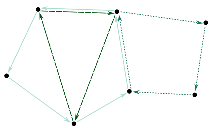
Figure 1. An example of a multigraph EμE^{\mu} constructed from one 33-directed cycle, one 44-directed cycle and one 55-directed cycle.

where card⁡(ν)\mathrm{card}(\nu) is the cardinality of ν\nu seen as a subset of 𝒞k1(n)×⋯×𝒞km(n)\mathcal{C}_{k_{1}}^{(n)}\times\dots\times\mathcal{C}_{k_{m}}^{(n)}. There is a natural inclusion map from 𝒯(k1,…,km)(n)\mathcal{T}_{(k_{1},\dots,k_{m})}^{(n)} into 𝒯(k1,…,km)(n+1)\mathcal{T}_{(k_{1},\dots,k_{m})}^{(n+1)} induced by the inclusion {1,…,n}⊂{1,…,n+1}\{1,\dots,n\}\subset\{1,\dots,n+1\} and these inclusions are surjective if n≥k1+⋯+kmn\geq k_{1}+\dots+k_{m}. With the help of these inclusions we can write, for n≥k1+⋯+kmn\geq k_{1}+\dots+k_{m},

1n(k1+⋯+km)/2​∑ν∈𝒯(k1,…,km)(n)card⁡(ν)​Wν=1n(k1+⋯+km)/2​∑μ∈𝒯(k1,…,km)(k1+⋯+km)cardn​(μ)​Wμ,\frac{1}{n^{(k_{1}+\dots+k_{m})/2}}\sum_{\nu\in\mathcal{T}_{(k_{1},\dots,k_{m})}^{(n)}}\mathrm{card}(\nu)W_{\nu}=\frac{1}{n^{(k_{1}+\dots+k_{m})/2}}\sum_{\mu\in\mathcal{T}_{(k_{1},\dots,k_{m})}^{(k_{1}+\dots+k_{m})}}\!\!\!\!\!\mathrm{card}_{n}\left(\mu\right)W_{\mu},

where cardn​(μ)\mathrm{card}_{n}\left(\mu\right) denotes the cardinality of μ\mu when seen as a subset of 𝒞k1(n)×⋯×𝒞km(n)\mathcal{C}_{k_{1}}^{(n)}\times\dots\times\mathcal{C}_{k_{m}}^{(n)}. So, it is enough to find the limit, as n→∞n\to\infty, of

cardn​(μ)n(k1+⋯+km)/2\frac{\mathrm{card}_{n}\left(\mu\right)}{n^{(k_{1}+\dots+k_{m})/2}}

for any μ∈𝒯(k1,…,km)(k1+⋯+km)\mu\in\mathcal{T}_{(k_{1},\dots,k_{m})}^{(k_{1}+\dots+k_{m})}. To understand better this cardinality, to each

μ=[(g1,…,gm)]∈𝒯(k1,…,km)(k1+⋯+km)\mu=[(g_{1},\dots,g_{m})]\in\mathcal{T}_{(k_{1},\dots,k_{m})}^{(k_{1}+\dots+k_{m})}

we associate the oriented multigraph GμG^{\mu} consisting of the union of the glg_{l}’s with edges counted multiple times (see Figure 1). More precisely, if VglV^{g_{l}} and EglE^{g_{l}} are the vertex set and the edge set of glg_{l}, then the vertex set VμV^{\mu} and the edge set EμE^{\mu} of GμG^{\mu} are

Vμ=⋃l=1mVglandEμ=⋃l=1m({l}×Egl)V^{\mu}=\bigcup_{l=1}^{m}V^{g_{l}}\quad\text{and}\quad E^{\mu}=\bigcup_{l=1}^{m}\left(\{l\}\times E^{g_{l}}\right)

with the source and target maps, s:Eμ→Vμs:E^{\mu}\to V^{\mu} and t:Eμ→Vμt:E^{\mu}\to V^{\mu}, defined by

s⁡(l,(i,j))=iandt⁡(l,(i,j))=j.s\big(l,(i,j)\big)=i\quad\text{and}\quad t\big(l,(i,j)\big)=j.

If there is an edge e∈Eμe\in E^{\mu} that is not multiple, in other words such that (s,t)​(e)≠(s,t)​(e′)(s,t)(e)\neq(s,t)(e^{\prime}) for every other edge e′≠ee^{\prime}\neq e, then Wμ=0W_{\mu}=0. So we consider only graphs where all edges are multiple. If for each v∈Vμv\in V^{\mu} the outer degree deg⁡(v)\mathrm{deg}(v) is defined by

deg⁡(v)=card⁡{e∈Eμ:s⁡(e)=v}\mathrm{deg}(v)=\mathrm{card}\{e\in E^{\mu}:s(e)=v\}

we have that deg⁡(v)≥2\mathrm{deg}(v)\geq 2 for every v∈Vμv\in V^{\mu}. By using the handshaking lemma, we have

∑v∈Vμdeg⁡(v)=card⁡(Eμ)=k1+⋯+km.\sum_{v\in V^{\mu}}\mathrm{deg}(v)=\mathrm{card}(E^{\mu})=k_{1}+\dots+k_{m}.

We notice that if, moreover, deg⁡(v∗)≥3\mathrm{deg}(v_{*})\geq 3 for some v∗∈Vμv_{*}\in V^{\mu} then

k1+⋯+km=∑v∈Vμ∖{v∗}deg⁡(v)+deg⁡(v∗)≥2​(card⁡(Vμ)−1)+3=2​card​(Vμ)+1k_{1}+\dots+k_{m}=\sum_{v\in V^{\mu}\setminus\{v_{*}\}}\mathrm{deg}(v)+\mathrm{deg}(v_{*})\geq 2\left(\mathrm{card}(V^{\mu})-1\right)+3=2\mathrm{card}(V^{\mu})+1

so that

card⁡(Vμ)<k1+⋯+km2.\mathrm{card}(V^{\mu})<\frac{k_{1}+\dots+k_{m}}{2}.

But cardn​(μ)≤ncard⁡(Vμ)\mathrm{card}_{n}(\mu)\leq n^{\mathrm{card}(V^{\mu})}, which implies that

cardn​(μ)n(k1+⋯+km)/2→n→∞0.\frac{\mathrm{card}_{n}(\mu)}{n^{(k_{1}+\dots+k_{m})/2}}\xrightarrow[n\to\infty]{}0.
Refer to caption
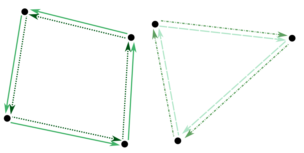
Figure 2. A graph formed by two 44-directed cycles and two 33-directed cycles satisfying the condition in (4.1).

Then, we suppose that deg⁡(v)=2\mathrm{deg}(v)=2 for every v∈Vμv\in V^{\mu}. Choose (g1,…,gm)(g_{1},\dots,g_{m}) such that [(g1,…,gm)]=μ[(g_{1},\dots,g_{m})]=\mu. By using that all edges of GμG^{\mu} are multiple and that every vertex has degree exactly 22 we can see that there must be a partition into pairs of {1,…,m}\{1,\dots,m\} such that (see Figure 2)

(4.1) gi=gjif ​i∼jandVgi∩Vgj=∅if ​i≁jg_{i}=g_{j}\quad\text{if }i\sim j\quad\text{and}\quad V^{g_{i}}\cap V^{g_{j}}=\emptyset\quad\text{if }i\not\sim j

where the relation ∼\sim denotes if the elements belong to the same set of the partition and VglV^{g_{l}} denotes the vertex set of glg_{l} as before. Necessarily mm is even and for each such μ\mu we have

cardn​(μ)n(k1+⋯+km)/2→n→∞1k1⋯km\frac{\mathrm{card}_{n}\left(\mu\right)}{n^{(k_{1}+\dots+k_{m})/2}}\xrightarrow[n\to\infty]{}\frac{1}{\sqrt{k}_{1}\cdots\sqrt{k}_{m}}

where the term k1⋯km\sqrt{k}_{1}\cdots\sqrt{k}_{m} appears because we are counting cycles with no distinguished vertex. There is precisely one μ\mu associated to any partition 𝒫\mathcal{P} into pairs of {1,…,m}\{1,\dots,m\} such that

(4.2) ki=kjif ​i∼j.k_{i}=k_{j}\quad\text{if }i\sim j.

Then, we shall use the notation W𝒫=WμW_{\mathcal{P}}=W_{\mu} to notice that

1n(k1+⋯+km)/2​∑μ∈𝒯(k1,…,km)k1+⋯+kmcardn​(μ)​Wμ→n→∞1k1⋯kn​∑𝒫W𝒫\frac{1}{n^{(k_{1}+\cdots+k_{m})/2}}\sum_{\mu\in\mathcal{T}_{(k_{1},\ldots,k_{m})}^{k_{1}+\cdots+k_{m}}}\mathrm{card}_{n}\left(\mu\right)W_{\mu}\xrightarrow[n\to\infty]{}\frac{1}{\sqrt{k}_{1}\cdots\sqrt{k}_{n}}\sum_{\mathcal{P}}W_{\mathcal{P}}

where the sum is over all partition into pairs of {1,…,m}\{1,\dots,m\} such that (4.2) happens. Since

W𝒫=∏𝔼⁡[αkisi​αkjsj],W_{\mathcal{P}}=\prod\mathbb{E}\left[\alpha_{k_{i}}^{s_{i}}\alpha_{k_{j}}^{s_{j}}\right],

where the product runs over all the pairs {i,j}\{i,j\} with i∼ji\sim j and i≠ji\neq j, and where αk=a12​a23​…​a(k−1)​k​ak​1\alpha_{k}=a_{12}a_{23}\dots a_{(k-1)k}a_{k1}. We may use Isserlis/Wick theorem to conclude.

4.5. Proof of Lemma 3.5

We start by checking that

(4.3) 𝔼⁡[rk(n)nk/2]→n→∞{𝔼​[a112]k/2if k is even0 if k is odd.\mathbb{E}\left[\frac{r_{k}^{(n)}}{n^{k/2}}\right]\xrightarrow[n\to\infty]{}\begin{cases}\mathbb{E}\left[{a_{11}}^{2}\right]^{k/2}&\text{if $k$ is even}\\ 0&\text{ if $k$ is odd.}\end{cases}

We may use the same kind of counting argument as in Lemma 3.4. Given a sequence (i1,…,ik)(i_{1},\dots,i_{k}), we construct a multigraph from it and notice that every edge must be multiple for the graph to contribute. Next, if some vertex has outer degree greater or equal than three then that graph does not contribute neither. Finally, if the graph constructed from (i1,…,ik)(i_{1},\dots,i_{k}) has every edge multiple and every vertex has outer degree two we can show that it is a double cycle (see Figure 3), in other words kk is even, and for l<l′l<l^{\prime} we have that

il=il′ if and only if l′=l+k2.i_{l}=i_{l^{\prime}}\quad\text{ if and only if }\quad l^{\prime}=l+\frac{k}{2}.

The expectation 𝔼⁡[ag]\mathbb{E}[a_{g}] for such double cycle gg is equal to 𝔼​[a112]k/2\mathbb{E}[a_{11}^{2}]^{k/2}. Since there are

n(n−1)…(n−k2+1)n(n-1)\dots\Bigr(n-\frac{k}{2}+1\Bigr)

of those (i1,…,ik)(i_{1},\dots,i_{k}), we have checked that (4.3) holds.

Refer to caption
Figure 3. A single graph formed by a double cycle that counts for obtaining the expected value.

Now, for any pair of square-integrable complex random variables XX and YY let us use the notation

cov⁡(X,Y)=𝔼⁡[(X−𝔼⁡[X])​(Y¯−𝔼⁡[Y¯])] while var⁡(X)=cov⁡(X,X)=𝔼⁡[|X−𝔼⁡[X]|2].\mathrm{cov}(X,Y)=\mathbb{E}\big[(X-\mathbb{E}[X])(\overline{Y}-\mathbb{E}[\overline{Y}])\big]\quad\mbox{ while }\quad\mathrm{var}(X)=\mathrm{cov}(X,X)=\mathbb{E}[|X-\mathbb{E}[X]|^{2}].

To complete the proof of Lemma 3.5, it is sufficient to prove that

(4.4) var⁡(rk(n)nk/2)→n→∞0.\mathrm{var}\left(\frac{r_{k}^{(n)}}{n^{k/2}}\right)\xrightarrow[n\to\infty]{}0.

To this end, if i=(i1,…,ik)i=(i_{1},\ldots,i_{k}), we set

ai=ai1​i2​ai2​i3​…​aik−1​ik​aik​i1.a_{i}=a_{i_{1}i_{2}}a_{i_{2}i_{3}}\dots a_{i_{k-1}i_{k}}a_{i_{k}i_{1}}.

By construction, we have

(4.5) var⁡(rk(n))=∑i,jcov⁡(ai,aj),\mathrm{var}\left(r_{k}^{(n)}\right)=\sum_{i,j}\mathrm{cov}\left(a_{i},a_{j}\right),

where the sum is over all pairs (i,j)(i,j) of kk-tuples such that both ii and jj have less than kk distinct elements.

From Cauchy – Schwarz inequality, the following crude bound holds:

|cov⁡(ai,aj)|≤4​M2​k,\left|\mathrm{cov}\left(a_{i},a_{j}\right)\right|\leq 4M^{2k},

where MM is such that the support of a11a_{11} is contained in the ball of radius MM. Also, as above, we may identify each kk-tuple ii with a path of length kk. Setting ik+1=i1i_{k+1}=i_{1}, let us introduce the set of visited vertices and the set of directed edges by

Vi={i1,…,ik}andEi={(il,il+1):l=1,…,k}.V_{i}=\{i_{1},\ldots,i_{k}\}\quad\text{and}\quad E_{i}=\{(i_{l},i_{l+1}):l=1,\ldots,k\}.

Then Gi=(Vi,Ei)G_{i}=(V_{i},E_{i}) is the directed graph associated to ii (self-loop edges allowed). We define its excess as

χi=card⁡(Ei)−card⁡(Vi)+1≥0.\chi_{i}=\mathrm{card}(E_{i})-\mathrm{card}(V_{i})+1\geq 0.

It is the minimal number of edges to be removed such that the remaining subgraph has no undirected cycle (with the convention that (u,u)(u,u) is a cycle of length 11 and for u≠vu\neq v, {(u,v),(v,u)}\{(u,v),(v,u)\} forms a cycle of length 22). Since GiG_{i} is the graph associated to a path of length kk, the assumption card⁡(Vi)<k\mathrm{card}(V_{i})<k implies that

χi≥2.\chi_{i}\geq 2.

Similarly, if i,ji,j are two kk-tuples, we consider their associated graph with vertex and directed edge sets

Vi​j=Vi∪VjandEi​j=Ei∪Ej.V_{ij}=V_{i}\cup V_{j}\quad\text{and}\quad E_{ij}=E_{i}\cup E_{j}.

The excess of the corresponding graph Gi​j=(Vi​j,Ei​j)G_{ij}=(V_{ij},E_{ij}) is

χi​j=card⁡(Ei​j)−card⁡(Vi​j)+c\chi_{ij}=\mathrm{card}(E_{ij})-\mathrm{card}(V_{ij})+c

where c∈{1,2}c\in\{1,2\} is the number of weak connected components of Gi​jG_{ij}: c=1c=1 if Vi∩Vj≠∅V_{i}\cap V_{j}\neq\emptyset and c=2c=2 otherwise. Since Gi​jG_{ij} is the union of GiG_{i} and GjG_{j}, we have

χi​j≥max⁡(χi,χj)≥2.\chi_{ij}\geq\max(\chi_{i},\chi_{j})\geq 2.

Now, from the independence of the entries of the matrix AnA_{n}, we have cov⁡(ai,aj)=0\mathrm{cov}(a_{i},a_{j})=0 unless Ei∩EjE_{i}\cap E_{j} is not empty. Thus Gi​jG_{ij} is connected for such i,ji,j. Moreover, cov⁡(ai,aj)=0\mathrm{cov}(a_{i},a_{j})=0 unless all edges of Ei​jE_{ij} are visited at least twice by the union of paths ii and jj. Hence, for such i,ji,j, card⁡(Ei​j)≤k\mathrm{card}(E_{ij})\leq k and thus

card⁡(Vi​j)=1−χi​j+card⁡(Ei​j)≤k−1.\mathrm{card}(V_{ij})=1-\chi_{ij}+\mathrm{card}(E_{ij})\leq k-1.

We thus have checked that

var⁡(rk(n))≤4​Ck​M2​k​nk−1,\mathrm{var}\left(r_{k}^{(n)}\right)\leq 4C_{k}M^{2k}n^{k-1},

where CkC_{k} bounds the number of possibilities for the pair of kk-tuples (i,j)(i,j) once the set Vi​jV_{ij} is chosen. This gives (4.4), which concludes the proof of the lemma.

References

  • [1] Zhi Dong Bai and Yong Quan Yin, Limiting behavior of the norm of products of random matrices and two problems of Geman-Hwang, Probab. Theory Related Fields 73 (1986), no. 4, 555–569. MR 863545
  • [2] Zhidong Bai and Jack W. Silverstein, Spectral analysis of large dimensional random matrices, second ed., Springer Series in Statistics, Springer, New York, 2010. MR 2567175
  • [3] Anirban Basak and Ofer Zeitouni, Outliers of random perturbations of Toeplitz matrices with finite symbols, Probab. Theory Related Fields 178 (2020), no. 3-4, 771–826. MR 4168388
  • [4] Charles Bordenave, Pietro Caputo, and Djalil Chafaï, Spectrum of non-Hermitian heavy tailed random matrices, Comm. Math. Phys. 307 (2011), no. 2, 513–560. MR 2837123
  • [5] Charles Bordenave, Pietro Caputo, Djalil Chafaï, and Konstantin Tikhomirov, On the spectral radius of a random matrix: an upper bound without fourth moment, Ann. Probab. 46 (2018), no. 4, 2268–2286. MR 3813992
  • [6] Charles Bordenave and Djalil Chafaï, Around the circular law, Probab. Surv. 9 (2012), 1–89. MR 2908617
  • [7] Raphaël Butez and David García-Zelada, Extremal particles of two-dimensional Coulomb gases and random polynomials on a positive background, arXiv:1811.12225v2, 2018.
  • [8] Giorgio Cipolloni, László Erdős, and Dominik Schröder, Central limit theorem for linear eigenvalue statistics of non-hermitian random matrices, preprint arXiv:1912.04100v5, 2019.
  • [9] by same author, Fluctuation around the circular law for random matrices with real entries, preprint arXiv:2002.02438v6, 2020.
  • [10] Stuart Geman, The spectral radius of large random matrices, Ann. Probab. 14 (1986), no. 4, 1318–1328. MR 866352
  • [11] Jean Ginibre, Statistical ensembles of complex, quaternion, and real matrices, J. Mathematical Phys. 6 (1965), 440–449. MR 173726
  • [12] Vyacheslav L. Girko, The circular law, Teor. Veroyatnost. i Primenen. 29 (1984), no. 4, 669–679. MR 773436
  • [13] by same author, From the first rigorous proof of the circular law in 1984 to the circular law for block random matrices under the generalized Lindeberg condition, Random Oper. Stoch. Equ. 26 (2018), no. 2, 89–116. MR 3808330
  • [14] J. Ben Hough, Manjunath Krishnapur, Yuval Peres, and Bálint Virág, Zeros of Gaussian analytic functions and determinantal point processes, University Lecture Series, vol. 51, American Mathematical Society, Providence, RI, 2009. MR 2552864
  • [15] Christopher P. Hughes, Jonathan P. Keating, and Neil O’Connell, On the characteristic polynomial of a random unitary matrix, Comm. Math. Phys. 220 (2001), no. 2, 429–451. MR 1844632
  • [16] Chii-Ruey Hwang, A brief survey on the spectral radius and the spectral distribution of large random matrices with i.i.d. entries, Random matrices and their applications (Brunswick, Maine, 1984), Contemp. Math., vol. 50, Amer. Math. Soc., Providence, RI, 1986, pp. 145–152. MR 841088
  • [17] Svante Janson and Krzysztof Nowicki, The asymptotic distributions of generalized UU-statistics with applications to random graphs, Probab. Theory Related Fields 90 (1991), no. 3, 341–375. MR 1133371
  • [18] Joseph Najnudel, Elliot Paquette, and Nick Simm, Secular coefficients and the holomorphic multiplicative chaos, preprint arXiv:2011.01823v1, 2020.
  • [19] B. Rider and Jack W. Silverstein, Gaussian fluctuations for non-Hermitian random matrix ensembles, Ann. Probab. 34 (2006), no. 6, 2118–2143. MR 2294978
  • [20] Tomoyuki Shirai, Limit theorems for random analytic functions and their zeros, Functions in number theory and their probabilistic aspects, RIMS Kôkyûroku Bessatsu, B34, Res. Inst. Math. Sci. (RIMS), Kyoto, 2012, pp. 335–359. MR 3014854
  • [21] Terence Tao and Van Vu, Random matrices: universality of ESDs and the circular law, Ann. Probab. 38 (2010), no. 5, 2023–2065, With an appendix by Manjunath Krishnapur. MR 2722794