跳到论文正文
W Papers独立论文阅读器 arXiv:2012.05591 论文正文 计算阅读时间 · 0%
引用这篇论文根据当前论文元数据生成,正式投稿前建议核对。


License: arXiv.org perpetual non-exclusive license
arXiv:2012.05591v2 [stat.ME] 14 Dec 2020

Efficient Learning for Clustering and Optimizing Context-Dependent Designs

Haidong Li    Henry Lam    Yijie Peng
Abstract

We consider a simulation optimization problem for a context-dependent decision-making. A Gaussian mixture model is proposed to capture the performance clustering phenomena of context-dependent designs. Under a Bayesian framework, we develop a dynamic sampling policy to efficiently learn both the global information of each cluster and local information of each design for selecting the best designs in all contexts. The proposed sampling policy is proved to be consistent and achieve the asymptotically optimal sampling ratio. Numerical experiments show that the proposed sampling policy significantly improves the efficiency in context-dependent simulation optimization.

keywords
simulation, ranking and selection, context, performance clustering
††runningauthor: Li, Lam and Peng††runningtitle: Efficient Learning for Clustering and Optimizing Context-Dependent Designs††authors: Department of Industrial Engineering and Management, College of Engineering, Peking University, Beijing 100871, China, haidong.li@pku.edu.cn Department of Industrial Engineering and Operations Research, Columbia University, NY 10027, USA, henry.lam@columbia.edu Department of Management Science and Information Systems, Guanghua School of Management, Peking University, Beijing 100871, China, pengyijie@pku.edu.cn ††affiliation: ††affiliation: ††affiliation: ††affiliation: ††affiliation: ††affiliation:

1 Introduction

Simulation is a powerful tool for optimizing complex stochastic systems. We consider a simulation optimization problem of selecting the best design under different contexts. The mean performances of each design under each context are unknown and can only be estimated via simulation. The performance of each design depends on the contexts, and thus the best design is also context-dependent. For example, in movie recommendation (Liu et al. 2009), movies and users can be regarded as designs and contexts, respectively. We aim to recommend the favorite movie for each user. Other examples include patient-specific treatment regimen-making (Kim et al. 2011) and automated asset management (Faloon and Scherer 2017).

For any fixed context, we aim to find the best design among a finite set of alternatives, which is referred to as ranking and selection (R&S) in the literature. R&S procedures intelligently allocate simulation replications to efficiently learn the best design. The probability of correct selection (PCS) is used as a measure to evaluate the efficiency of sampling procedure in R&S. In our problem, the best design is not universal but context-dependent. In this work, the goal is to correctly select all best designs in each context. Besides determining how to allocate simulation replications among different designs in a context, our sampling procedure also needs to consider simulation budget allocation among different contexts since incorrect selection in any context can lead to the failure of our goal. The worst-case notion is used to describe the context with the lowest PCS, and the worst-case probability of correct selection (PCSW\text{PCS}_{\text{W}}) under all contexts is used to measure the efficiency of sampling procedure in our problem.

In R&S, the efficiency in sampling for learning the best design is a central issue, because simulation is usually expensive and there could be a large number of possible designs. In our problem, the learning efficiency is more important because there could also exist a large number of possible contexts, and the number of all design-context pairs is a multiplication of the number of designs and the number of contexts. The complexity of the optimization problem can be substantially reduced if the performance cluster information in designs and contexts can be appropriately utilized. In the movie recommendation example, tremendous movies can be classified into a few categories such as drama, comedy, and action, and countless users can also be characterized by a relatively small number of attributes such as age, gender, and occupation. Users with a common attribute tend to favor movies in certain categories, e.g., arguably young people on average rate action movies higher than senior people, so the performance clustering phenomenon exists in the design-context pairs for the movie recommendation problem. The performance clustering phenomena are rather common in combinatorial optimization problems with many application backgrounds including manufacturing and healthcare (Peng et al. 2019).

Accurately identifying the performance clusters would simplify the optimization problem, because designs in a cluster tend to have similar performances while designs in different clusters typically have significant differences in their performances, which provides useful global information for learning the best designs. However, the performances of the designs are estimated by random sampling in simulation, so how to efficiently learn the performance cluster information by sampling is an important issue for our problem.

To capture the performance clustering phenomena, we use a Gaussian mixture model as the prior distribution for the performance of a design-context pair, and the hyper-parameters in the prior distribution are estimated from sampling information. Under a Bayesian framework, we formulate the sequential sampling decision as a stochastic dynamic programming problem, and provide an efficient scheme to update the posterior information for each design-context pair. Moreover, we propose a dynamic sampling policy based on the sequentially updated posterior information to efficiently learn both the global information of each cluster and local information of each design. The proposed sampling policy is proved to be consistent and achieve the asymptotically optimal sampling ratio. The contribution of our work is threefold.

  • •

    We consider performance clustering in design-context pairs to enhance the efficiency for learning the best designs in all contexts.

  • •

    We provide an efficient scheme to simultaneously learn the global clustering information and local performance information in design-context pairs.

  • •

    We propose an efficient dynamic sampling procedure for context-dependent simulation optimization, which is proved to be asymptotically optimal.

1.1 Related Literature

The R&S literature consists of the frequentist and the Bayesian branches. See Kim and Nelson 2006 and Chen et al. 2015 for overviews. Frequentist procedures (e.g., Rinott 1978, Kim and Nelson 2001, Luo et al. 2015) allocate simulation replications to guarantee a pre-specified PCS level, whereas Bayesian procedures (e.g. Chen et al. 2000, Chick and Frazier 2012, Gao et al. 2017a) aim to either maximize the PCS or minimize the expected opportunity cost subject to a given simulation budget. Bayesian procedures usually achieve better performance than frequentist procedures under a given simulation budget, but they typically do not provide a guaranteed PCS. Peng et al. 2019 offered an off-line learning scheme to extract clustering information from auxiliary information of the low-fidelity models in a classic R&S setting, whereas our work proposes an on-line learning algorithm for simultaneously clustering and optimizing context-dependent designs.

The literature on context-dependent simulation optimization is sparse relative to the actively studied R&S problem in simulation. Contexts are also known as the covariates, side information, or auxiliary quantities. To the best of our knowledge, the study of Shen et al. 2017 is the first research for this problem. They assume a linear relationship between the response of a design and the contexts, and develop sampling procedures to provide a guarantee on PCS for all contexts. Li et al. 2018 further extend the result in Shen et al. 2017 to high-dimensional contexts and general dependence between the mean performance of a design and the contexts. The aforementioned two studies adopt the Indifference Zone paradigm in the frequentist branch. Gao et al. 2019 adopted an optimal computing budget allocation (OCBA) approach in R&S, and solve the problem by identifying the rate-optimal budget allocation rule. None of the existing work formulates the sequential sampling decision as a stochastic dynamic programming problem and considers the performance clustering in design-context pairs.

Our work is related to the literature on contextual multi-arm bandit (MAB) problem in machine learning. In the MAB problem, a fixed amount of samples are allocated to competing alternatives for maximizing their cumulative expected reward (Bubeck et al. 2012). In our problem, similar to a pure-exploration version of MAB known as the best-arm identification problem, the reward only appears in the final stage for selecting the best designs. Auer 2000 and Hong et al. 2011 assume a linear dependency between context and the expected reward of an action to provide an approximate solution for the contextual MAB problem. Nonlinear contextual reward functions approximated by nonparametric regression, random forest, and neural network can be found in Rigollet and Zeevi 2010, Slivkins 2014, Perchet et al. 2013, Allesiardo et al. 2014, Féraud et al. 2016. Han et al. 2020 study sequential batch learning in the adversarial contexts and linear rewards setting. Choosing contexts adversarially allows the decision maker learn knowledge about the rewards as few as possible, which can be considered as the worst case. However, relatively few studies exist on contextual best-arm identification. All analysis of best-arm identification in Soare et al. 2014, Xu et al. 2018, and Kazerouni and Wein 2019 assume a linear or generalized linear dependence of rewards on the contexts. None of studies on MAB exploit clustering information in context-dependent designs.

Optimizing the worst-case performance over a range of scenarios when facing model ambiguity is a theme of robust optimization (RO); see Ben-Tal et al. 2009 and Bertsimas et al. 2011 for an introduction. In the simulation literature, the so-call robust simulation applies worst-case analysis on a simulation model when the input distribution is uncertain but postulated to lie within a set, see, e.g., Hu et al. 2012, Glasserman and Xu 2014, Hu and Hong 2015, Lam 2016, Lam 2018, Ghosh and Lam 2019. Focusing on the worst-case calculation, the decision variables in the resulting optimization in these works are the unknown input distributions. In contrast, our approach involves optimizing design variables on a criterion that uses the worst-case performance. This is closer to Hu and Hong 2013 and Fan et al. 2020 that consider decision-making over the worst-case scenario in simulation contexts. However, in these works, the performance of each design is context-dependent while the goal is to find a design with the best worst-case performance, whereas in our problem the best design is also context-dependent.

The rest of the paper is organized as follows. In Section 2, we formulate the studied problem and introduce assumptions of this research. Section 3 derives the posterior estimates of parameters in the Gaussian mixture model. In Section 4, we develop a dynamic sampling procedure. Section 5 presents numerical examples and computational results, and Section 6 concludes the paper and outlines future directions. The proofs of the theorems and propositions in the paper can be found in the online appendix.

2 Problem Description

Suppose there are nn different designs. For i=1,…,ni=1,\ldots,n, the performance yi​(𝒙)y_{i}(\bm{x}) of design ii depends on a vector of context 𝒙=(x1,…,xd)⊤\bm{x}=(x_{1},\ldots,x_{d})^{\top} for 𝒙∈𝒳⊆ℝd\bm{x}\in\mathcal{X}\subseteq\mathbb{R}^{d}. The performances are unknown and can only be learned via sampling. In this study, we assume that 𝒳\mathcal{X} contains a finite number of mm possible contexts 𝒙1,…,𝒙m\bm{x}_{1},\ldots,\bm{x}_{m}. Our objective is to correctly select the best design for a given value of 𝒙\bm{x} (see Figure 1 for an illustration), i.e., identify arg⁡maxi​yi​(𝒙){\arg\max}_{i}\ y_{i}(\bm{x}). For example, in personalized movie recommendation, we aim to recommend the most favorite movie (design) for the corresponding user (context). Since sampling could be expensive, the total number of samples is usually limited. Moreover, when either nn or mm is relatively large, it would be practically infeasible to estimate all performances accurately for each design ii and each context 𝒙j\bm{x}_{j}.

Refer to caption
Figure 1: Selecting the best (red) design under each context.

Under a fixed context 𝒙\bm{x}, the quality of the selection for the best design is measured by the probability of correct selection (PCS),

PCS​(𝒙)=ℙ⁡(⋂i≠i^∗​(𝒙)(y^i​(𝒙)<y^i^∗​(𝒙)​(𝒙))),\text{PCS}(\bm{x})=\mathbb{P}\left(\bigcap_{i\neq\widehat{i}^{*}(\bm{x})}\left(\widehat{y}_{i}(\bm{x})<\widehat{y}_{\widehat{i}^{*}(\bm{x})}(\bm{x})\right)\right),

where i^∗​(𝒙)\widehat{i}^{*}(\bm{x}) is the estimated best design and y^i​(𝒙)\widehat{y}_{i}(\bm{x}) is the posterior performance for design ii and context 𝒙\bm{x}. In this study, we aim to provide the best design for all the 𝒙\bm{x} that might possibly appear, and therefore need a measure for evaluating the quality of the selection over the entire context space 𝒳\mathcal{X}. Specifically, we adopt the worst-case probability of correct selection over 𝒳\mathcal{X}:

PCSW=min𝒙∈𝒳​PCS​(𝒙).\text{PCS}_{\text{W}}=\underset{\bm{x}\in\mathcal{X}}{\min}\ \text{PCS}(\bm{x}).

This measure has been used in contextual R&S (Gao et al. 2019), and uses the worst-case notion in robust optimization (Bertsimas et al. 2011) and R&S with input uncertainty (Gao et al. 2017b).

2.1 Assumption

We assume that for each design and context, the simulation observations are i.i.d. normally distributed, i.e., Yi,t​(𝒙)∼N⁡(yi​(𝒙),σi2​(𝒙))Y_{i,t}(\bm{x})\sim N(y_{i}(\bm{x}),\sigma_{i}^{2}(\bm{x})), i=1,…,ni=1,\ldots,n, t∈ℤ+t\in\mathbb{Z}^{+}, 𝒙∈𝒳\bm{x}\in\mathcal{X}, and the replications among different designs and different contexts are independent. The variance σi2​(𝒙)\sigma_{i}^{2}(\bm{x}) in the sampling distribution is assumed to be known in this study and use the sample estimate as a plug-in for the true value in practice. We use ϕ(⋅|μ,σ2)\phi(\cdot|\mu,\sigma^{2}) to denote the density of a normal distribution with mean μ\mu and variance σ2\sigma^{2}. The normal assumption is the most common assumption in R&S research. For non-normal sampling distributions, the normal assumption is justified by the use of batching (Kim and Nelson 2006).

Refer to caption
Figure 2: The performance clustering phenomenon in designs and contexts.

A Bayesian framework is introduced in learning the unknown performances of different designs under different contexts, and the prior distribution of yi​(𝒙)y_{i}(\bm{x}) is assumed to be a Gaussian mixture distribution:

yi(𝒙)∼∑k=1K∑ℓ=1Lτkωℓϕ(⋅|μk​ℓ,σk​ℓ2),y_{i}(\bm{x})\sim\sum_{k=1}^{K}\sum_{\ell=1}^{L}\tau_{k}\omega_{\ell}\phi(\cdot|\mu_{k\ell},\sigma_{k\ell}^{2}),

where KK is the (unknown) number of clusters in design dimension, LL is the (unknown) number of clusters in context dimension, τk\tau_{k} is the unknown (probability) weight of the kk-th cluster in design dimension, ωℓ\omega_{\ell} is the unknown (probability) weight of the ℓ\ell-th cluster in context dimension, and ϕ(⋅|μk​ℓ,σk​ℓ2)\phi(\cdot|\mu_{k\ell},\sigma_{k\ell}^{2}) is the density of each mixture component. The Gaussian mixture model prior distribution reflects the performance clustering phenomenon in designs and contexts. For example, design performances are similar in each block as shown in Figure 2, that is to say, the users in the same cluster have similar preferences on the movies in the same cluster. In cases without a clear performance clustering structure, our prior distribution would then have only one component and reduce to the widely used normal prior distribution in Bayesian R&S literature. When there is only one context, we simply consider the performance clustering phenomenon in designs, and our prior distribution reduces to the special case in Peng et al. 2019.

3 Parameter Estimation

To extract the information of performance clustering from observations, we introduce two hidden state random variables zi=(zi,1,…,zi,K)z_{i}=(z_{i,1},\ldots,z_{i,K}) and vj=(vj,1,…,vj,L)v_{j}=(v_{j,1},\ldots,v_{j,L}), which follow multinomial distributions:

p⁡(zi)=∏k=1Kτkzi,k,\displaystyle p(z_{i})=\prod_{k=1}^{K}\tau_{k}^{z_{i,k}},
p⁡(vj)=∏ℓ=1Lωℓvj,ℓ,\displaystyle p(v_{j})=\prod_{\ell=1}^{L}\omega_{\ell}^{v_{j,\ell}},
s.t.∑k=1Kzi,k=1,zi,k∈{0,1},k=1,…,K,\displaystyle s.t.\ \sum_{k=1}^{K}z_{i,k}=1,\ z_{i,k}\in\{0,1\},\ k=1,\ldots,K,
∑ℓ=1Lvj,ℓ=1,vj,ℓ∈{0,1},ℓ=1,…,L.\displaystyle\ \ \ \ \sum_{\ell=1}^{L}v_{j,\ell}=1,\ v_{j,\ell}\in\{0,1\},\ \ell=1,\ldots,L.

The hidden state random variable zi,kz_{i,k} assigns design ii to cluster kk if zi,k=1z_{i,k}=1 while the hidden state random variable vj,ℓv_{j,\ell} assigns context jj to cluster ℓ\ell if vj,ℓ=1v_{j,\ell}=1, which means yi​(𝒙j)y_{i}(\bm{x}_{j}) comes from a realization of distribution ϕ(⋅|μk​ℓ,σk​ℓ2)\phi(\cdot|\mu_{k\ell},\sigma_{k\ell}^{2}).

Let ti​jt_{ij} be the number of simulation replications allocated to design ii in context jj after allocating a total amount of tt simulation replications. To obtain the posterior statistics of the unobservable performance 𝒚=[yi​(𝒙j)]n×m\bm{y}=[y_{i}(\bm{x}_{j})]_{n\times m}, we introduce the likelihoods of observations ℰt={Yi,h​(𝒙j)}i=1,j=1,h=1n,m,ti​j\mathcal{E}_{t}=\{Y_{i,h}(\bm{x}_{j})\}_{i=1,j=1,h=1}^{n,m,t_{ij}} and unobservable Z=[zi,k]n×KZ=[z_{i,k}]_{n\times K} and V=[vj,ℓ]m×LV=[v_{j,\ell}]_{m\times L}. Given parameter θ={τk,ωℓ,μk​ℓ,σk​ℓ}k=1,ℓ=1K,L\theta=\{\tau_{k},\omega_{\ell},\mu_{k\ell},\sigma_{k\ell}\}_{k=1,\ell=1}^{K,L},

ℒ⁡(Z,θ)=∏i=1np⁡(zi)=∏i=1n∏k=1Kτkzi,k\mathcal{L}(Z;\theta)=\prod_{i=1}^{n}p(z_{i})=\prod_{i=1}^{n}\prod_{k=1}^{K}\tau_{k}^{z_{i,k}}

and

ℒ⁡(V,θ)=∏j=1mp⁡(vj)=∏j=1m∏ℓ=1Lωℓvj,ℓ\mathcal{L}(V;\theta)=\prod_{j=1}^{m}p(v_{j})=\prod_{j=1}^{m}\prod_{\ell=1}^{L}\omega_{\ell}^{v_{j,\ell}}

are the likelihood of design clustering state variable ZZ and context clustering state variable VV, respectively, the likelihood of true performance 𝒚\bm{y} given the clustering state variables ZZ and VV is

ℒ⁡(𝒚|Z,V;θ)=∏i=1n∏j=1m(∏k=1K∏ℓ=1L(ϕ⁡(yi​(𝒙j)|μk​ℓ,σk​ℓ2))zi,k​vj,ℓ),\mathcal{L}(\bm{y}|Z,V;\theta)=\prod_{i=1}^{n}\prod_{j=1}^{m}\left(\prod_{k=1}^{K}\prod_{\ell=1}^{L}\left(\phi\left(y_{i}(\bm{x}_{j})|\mu_{k\ell},\sigma_{k\ell}^{2}\right)\right)^{z_{i,k}v_{j,\ell}}\right),

and the likelihood of samples given the true performance 𝒚\bm{y} is

ℒ⁡(ℰt|𝒚;θ)=∏i=1n∏j=1m(∏h=1ti​jϕ⁡(Yi,h​(𝒙j)|yi​(𝒙j),σi2​(𝒙j))).\displaystyle\mathcal{L}(\mathcal{E}_{t}|\bm{y};\theta)=\prod_{i=1}^{n}\prod_{j=1}^{m}\left(\prod_{h=1}^{t_{ij}}\phi\left(Y_{i,h}(\bm{x}_{j})|y_{i}(\bm{x}_{j}),\sigma_{i}^{2}(\bm{x}_{j})\right)\right).

The likelihood of complete state variables, i.e., ℰt\mathcal{E}_{t}, 𝒚\bm{y}, ZZ, and VV, is

ℒ⁡(ℰt,𝒚,Z,V,θ)=ℒ⁡(Z,θ)​ℒ​(V,θ)​ℒ​(𝒚|Z,V;θ)​ℒ​(ℰt|𝒚;θ).\displaystyle\mathcal{L}(\mathcal{E}_{t},\bm{y},Z,V;\theta)=\mathcal{L}(Z;\theta)\mathcal{L}(V;\theta)\mathcal{L}(\bm{y}|Z,V;\theta)\mathcal{L}(\mathcal{E}_{t}|\bm{y};\theta).

The likelihood of observations ℰt\mathcal{E}_{t} is obtained by integrating out the unobservable state 𝒚\bm{y}, ZZ, and VV, which is given by

ℒ(ℰt;θ)=∑k1:n∈𝒦∑ℓ1:m∈ℒfτ(k1:n)fω(ℓ1:m)fY(ℰt|k1:n,ℓ1:m),\displaystyle\mathcal{L}(\mathcal{E}_{t};\theta)=\sum_{k_{1:n}\in\mathcal{K}}\sum_{\ell_{1:m}\in\mathcal{L}}f_{\tau}(k_{1:n})f_{\omega}(\ell_{1:m})f_{Y}(\mathcal{E}_{t}|k_{1:n},\ell_{1:m}),

where k1:nk_{1:n} is the design clustering index set such that zi,ki=1,ki∈𝒦≜{1,…,K}z_{i,k_{i}}=1,\ k_{i}\in\mathcal{K}\triangleq\{1,\ldots,K\}, ℓ1:m\ell_{1:m} is the context clustering index set such that vj,ℓj=1,ℓj∈ℒ≜{1,…,L}v_{j,\ell_{j}}=1,\ \ell_{j}\in\mathcal{L}\triangleq\{1,\ldots,L\}, the probability of design clustering situation k1:nk_{1:n} is

fτ(k1:n)≜∏i=1nτki,f_{\tau}(k_{1:n})\triangleq\prod_{i=1}^{n}\tau_{k_{i}},

the probability of context clustering situation ℓ1:m\ell_{1:m} is

fω(ℓ1:m)≜∏j=1mωℓj,f_{\omega}(\ell_{1:m})\triangleq\prod_{j=1}^{m}\omega_{\ell_{j}},

and the probability density of samples given k1:nk_{1:n} and ℓ1:m\ell_{1:m} is

fY(ℰt|k1:n,ℓ1:m)≜∏i=1n∏j=1mCi​j,ki​ℓj,f_{Y}(\mathcal{E}_{t}|k_{1:n},\ell_{1:m})\triangleq\prod_{i=1}^{n}\prod_{j=1}^{m}C_{ij,k_{i}\ell_{j}},

with

Ci​j,ki​ℓj≜∫ℝϕ⁡(yi​(𝒙j)|μki​ℓj,σki​ℓj2)​∏h=1ti​jϕ⁡(Yi,h​(𝒙j)|yi​(𝒙𝒋),σi2​(𝒙𝒋))​d​yi​(𝒙j).\displaystyle C_{ij,k_{i}\ell_{j}}\triangleq\int_{\mathbb{R}}\phi\left(y_{i}(\bm{x}_{j})|\mu_{k_{i}\ell_{j}},\sigma_{k_{i}\ell_{j}}^{2}\right)\prod_{h=1}^{t_{ij}}\phi\left(Y_{i,h}(\bm{x}_{j})|y_{i}(\bm{x_{j}}),\sigma_{i}^{2}(\bm{x_{j}})\right)dy_{i}(\bm{x}_{j}).

3.1 Number of Clusters

First, we need to determine numbers of clusters (KK and LL) in the mixture model. Specifically, KK and LL can be determined by using the Bayesian information criterion (BIC):

(K^,L^)=arg⁡maxK,L​[2​log⁡ℒ⁡(ℰt,θ^K,L)−(2​K​L+K+L)​log⁡(n​m)],\displaystyle(\widehat{K},\widehat{L})=\underset{K,L}{\arg\max}\ \left[2\log\mathcal{L}(\mathcal{E}_{t};\widehat{\theta}_{K,L})-(2KL+K+L)\log(nm)\right], (1)

where

θ^K,L=arg⁡max𝜃​ℒ​(ℰt,θ).\widehat{\theta}_{K,L}=\underset{\theta}{\arg\max}\ \mathcal{L}(\mathcal{E}_{t};\theta).

BIC includes a penalty term (2​K​L+K+L)​log⁡(n​m)(2KL+K+L)\log(nm) for the number of estimated parameters in the model to discount the log-likelihood which captures the statistical fitness. It is always possible to improve the statistical fitness with the data by choosing a more complex model with more parameters, but increased complexity in modeling may result in overfitting. For the Gaussian mixture model, the EM algorithm is one of the most popular methods to efficiently compute the MLE. Given an arbitrary initial value θ(0)\theta^{(0)}, the EM algorithm iteratively executes the following two steps:

  • •

    Expectation step (E-step): given ℰt\mathcal{E}_{t} under the current parameter estimate θ(s)\theta^{(s)}, calculate

    𝒬(θ|θ(s))≜𝔼[logℒ(ℰt,𝒚,Z,V;θ)|ℰt,θ(s)];\displaystyle\mathcal{Q}(\theta|\theta^{(s)})\triangleq\mathbb{E}\left[\log\mathcal{L}(\mathcal{E}_{t},\bm{y},Z,V;\theta)|\mathcal{E}_{t},\theta^{(s)}\right]; (2)
  • •

    Maximization step (M-step): maximize function 𝒬(⋅|θ(s))\mathcal{Q}(\cdot|\theta^{(s)}) to update the parameter estimate

    θ(s+1)=arg⁡max𝜃​𝒬​(θ|θ(s)).\displaystyle\theta^{(s+1)}=\underset{\theta}{\arg\max}\mathcal{Q}(\theta|\theta^{(s)}). (3)

3.2 Posterior Estimates

We provide a theorem for updating the clustering statistics and the posterior parameter estimates based on the EM algorithm. To start with, we provide a list of the notations.

  • ss

    the iteration number of the EM algorithm;

  • θ^(t,s)\widehat{\theta}^{(t,s)}

    the parameter estimates in the ss-th iteration of the EM algorithm conditional on ℰt\mathcal{E}_{t}, which includes elements τ^k(t,s)\widehat{\tau}_{k}^{(t,s)}, ω^ℓ(t,s)\widehat{\omega}_{\ell}^{(t,s)}, μ^k​ℓ(t,s)\widehat{\mu}_{k\ell}^{(t,s)}, and (σ^k​ℓ2)(t,s)(\widehat{\sigma}_{k\ell}^{2})^{(t,s)};

  • μi​j,k​ℓ(t,s)\mu_{ij,k\ell}^{(t,s)}

    the posterior mean of yi​(𝒙j)y_{i}(\bm{x}_{j}) conditional on {zi,k=1}\{z_{i,k}=1\}, {vj,ℓ=1}\{v_{j,\ell}=1\}, ℰt\mathcal{E}_{t}, and given θ^(t,s)\widehat{\theta}^{(t,s)};

  • (σi​j,k​ℓ2)(t,s)(\sigma_{ij,k\ell}^{2})^{(t,s)}

    the posterior variance of yi​(𝒙j)y_{i}(\bm{x}_{j}) conditional on {zi,k=1}\{z_{i,k}=1\}, {vj,ℓ=1}\{v_{j,\ell}=1\}, ℰt\mathcal{E}_{t}, and given θ^(t,s)\widehat{\theta}^{(t,s)}.

Theorem 3.1

The posterior distribution of yi​(𝐱j)y_{i}(\bm{x}_{j}) conditional on {zi,k=1}\{z_{i,k}=1\}, {vj,ℓ=1}\{v_{j,\ell}=1\}, ℰt\mathcal{E}_{t}, and given θ^(t,s)\widehat{\theta}^{(t,s)} is

ϕ⁡(yi​(𝒙j)|μi​j,k​ℓ(t,s),(σi​j,k​ℓ2)(t,s)),\phi(y_{i}(\bm{x}_{j})|\mu_{ij,k\ell}^{(t,s)},(\sigma_{ij,k\ell}^{2})^{(t,s)}),

where

(σi​j,ki​ℓj2)(t,s)=1/[ti​jσi2​(𝒙j)+1(σ^ki​ℓj2)(t,s)],\displaystyle(\sigma_{ij,k_{i}\ell_{j}}^{2})^{(t,s)}=1\Big/\left[\frac{t_{ij}}{\sigma_{i}^{2}(\bm{x}_{j})}+\frac{1}{(\widehat{\sigma}_{k_{i}\ell_{j}}^{2})^{(t,s)}}\right], (4)
μi​j,ki​ℓj(t,s)=(σi​j,ki​ℓj2)(t,s)​[∑h=1ti​jYi,h​(𝒙j)σi2​(𝒙j)+μ^ki​ℓj(t,s)(σ^ki​ℓj2)(t,s)];\displaystyle\mu_{ij,k_{i}\ell_{j}}^{(t,s)}=(\sigma_{ij,k_{i}\ell_{j}}^{2})^{(t,s)}\left[\frac{\sum_{h=1}^{t_{ij}}Y_{i,h}(\bm{x}_{j})}{\sigma_{i}^{2}(\bm{x}_{j})}+\frac{\widehat{\mu}_{k_{i}\ell_{j}}^{(t,s)}}{(\widehat{\sigma}_{k_{i}\ell_{j}}^{2})^{(t,s)}}\right]; (5)

the posterior probability of {zi,k=1}\{z_{i,k}=1\} conditional on ℰt\mathcal{E}_{t} and given θ^(t,s)\widehat{\theta}^{(t,s)} is

z^i,k(t,s)=∑k1:n∈𝒦,ki=k∑ℓ1:m∈ℒfτ(t,s)(k1:n)fω(t,s)(ℓ1:m)fY(t,s)(ℰt|k1:n,ℓ1:m)∑k1:n∈𝒦∑ℓ1:m∈ℒfτ(t,s)(k1:n)fω(t,s)(ℓ1:m)fY(t,s)(ℰt|k1:n,ℓ1:m),\displaystyle\widehat{z}_{i,k}^{(t,s)}=\frac{\sum_{k_{1:n}\in\mathcal{K},k_{i}=k}\sum_{\ell_{1:m}\in\mathcal{L}}f_{\tau}^{(t,s)}(k_{1:n})f_{\omega}^{(t,s)}(\ell_{1:m})f_{Y}^{(t,s)}(\mathcal{E}_{t}|k_{1:n},\ell_{1:m})}{\sum_{k_{1:n}\in\mathcal{K}}\sum_{\ell_{1:m}\in\mathcal{L}}f_{\tau}^{(t,s)}(k_{1:n})f_{\omega}^{(t,s)}(\ell_{1:m})f_{Y}^{(t,s)}(\mathcal{E}_{t}|k_{1:n},\ell_{1:m})}, (6)

the posterior probability of {vj,ℓ=1}\{v_{j,\ell}=1\} conditional on ℰt\mathcal{E}_{t} and given θ^(t,s)\widehat{\theta}^{(t,s)} is

v^j,ℓ(t,s)=∑k1:n∈𝒦∑ℓ1:m∈ℒ,ℓj=ℓfτ(t,s)(k1:n)fω(t,s)(ℓ1:m)fY(t,s)(ℰt|k1:n,ℓ1:m)∑k1:n∈𝒦∑ℓ1:m∈ℒfτ(t,s)(k1:n)fω(t,s)(ℓ1:m)fY(t,s)(ℰt|k1:n,ℓ1:m),\displaystyle\widehat{v}_{j,\ell}^{(t,s)}=\frac{\sum_{k_{1:n}\in\mathcal{K}}\sum_{\ell_{1:m}\in\mathcal{L},\ell_{j}=\ell}f_{\tau}^{(t,s)}(k_{1:n})f_{\omega}^{(t,s)}(\ell_{1:m})f_{Y}^{(t,s)}(\mathcal{E}_{t}|k_{1:n},\ell_{1:m})}{\sum_{k_{1:n}\in\mathcal{K}}\sum_{\ell_{1:m}\in\mathcal{L}}f_{\tau}^{(t,s)}(k_{1:n})f_{\omega}^{(t,s)}(\ell_{1:m})f_{Y}^{(t,s)}(\mathcal{E}_{t}|k_{1:n},\ell_{1:m})}, (7)

where

fτ(t,s)(k1:n)≜∏i=1nτ^ki(t,s),fω(t,s)(ℓ1:m)≜∏j=1mω^ℓj(t,s),f_{\tau}^{(t,s)}(k_{1:n})\triangleq\prod_{i=1}^{n}\widehat{\tau}_{k_{i}}^{(t,s)},\quad f_{\omega}^{(t,s)}(\ell_{1:m})\triangleq\prod_{j=1}^{m}\widehat{\omega}_{\ell_{j}}^{(t,s)},

and

fY(t,s)(ℰt|k1:n,ℓ1:m)≜∏i=1n∏j=1mCi​j,ki​ℓj(t,s)f_{Y}^{(t,s)}(\mathcal{E}_{t}|k_{1:n},\ell_{1:m})\triangleq\prod_{i=1}^{n}\prod_{j=1}^{m}C_{ij,k_{i}\ell_{j}}^{(t,s)}

with

Ci​j,ki​ℓj(t,s)≜(12​π​σi2​(𝒙j))ti​j2​(σi​j,ki​ℓj2)(t,s)(σ^ki​ℓj2)(t,s)​exp⁡{12​[(μi​j,ki​ℓj(t,s))2(σi​j,ki​ℓj2)(t,s)−∑h=1ti​jYi,h2​(𝒙j)σi2​(𝒙j)−(μ^ki​ℓj(t,s))2(σ^ki​ℓj2)(t,s)]}.C_{ij,k_{i}\ell_{j}}^{(t,s)}\triangleq\left(\frac{1}{2\pi\sigma_{i}^{2}(\bm{x}_{j})}\right)^{\frac{t_{ij}}{2}}\sqrt{\frac{(\sigma_{ij,k_{i}\ell_{j}}^{2})^{(t,s)}}{(\widehat{\sigma}_{k_{i}\ell_{j}}^{2})^{(t,s)}}}\exp\left\{\frac{1}{2}\left[\frac{(\mu_{ij,k_{i}\ell_{j}}^{(t,s)})^{2}}{(\sigma_{ij,k_{i}\ell_{j}}^{2})^{(t,s)}}-\frac{\sum_{h=1}^{t_{ij}}Y_{i,h}^{2}(\bm{x}_{j})}{\sigma_{i}^{2}(\bm{x}_{j})}-\frac{(\widehat{\mu}_{k_{i}\ell_{j}}^{(t,s)})^{2}}{(\widehat{\sigma}_{k_{i}\ell_{j}}^{2})^{(t,s)}}\right]\right\}.

The estimates of the parameters in the (s+1)(s+1)-th iteration of the EM algorithm are given by

τ^k(t,s+1)=∑i=1nz^i,k(t,s)n,ω^ℓ(t,s+1)=∑j=1mv^j,ℓ(t,s)m,\displaystyle\widehat{\tau}_{k}^{(t,s+1)}=\frac{\sum_{i=1}^{n}\widehat{z}_{i,k}^{(t,s)}}{n},\ \widehat{\omega}_{\ell}^{(t,s+1)}=\frac{\sum_{j=1}^{m}\widehat{v}_{j,\ell}^{(t,s)}}{m}, (8)
μ^k​ℓ(t,s+1)=∑i=1n∑j=1mz^i,k(t,s)​v^j,ℓ(t,s)​μi​j,k​ℓ(t,s)∑i=1n∑j=1mz^i,k(t,s)​v^j,ℓ(t,s),\displaystyle\widehat{\mu}_{k\ell}^{(t,s+1)}=\frac{\sum_{i=1}^{n}\sum_{j=1}^{m}\widehat{z}_{i,k}^{(t,s)}\widehat{v}_{j,\ell}^{(t,s)}\mu_{ij,k\ell}^{(t,s)}}{\sum_{i=1}^{n}\sum_{j=1}^{m}\widehat{z}_{i,k}^{(t,s)}\widehat{v}_{j,\ell}^{(t,s)}}, (9)

and

(σ^k​ℓ2)(t,s+1)=∑i=1n∑j=1mz^i,k(t,s)​v^j,ℓ(t,s)​[(σi​j,k​ℓ2)(t,s)+(μi​j,k​ℓ(t,s)−μ^k​ℓ(t,s+1))2]∑i=1n∑j=1mz^i,k(t,s)​v^j,ℓ(t,s).\displaystyle(\widehat{\sigma}_{k\ell}^{2})^{(t,s+1)}=\frac{\sum_{i=1}^{n}\sum_{j=1}^{m}\widehat{z}_{i,k}^{(t,s)}\widehat{v}_{j,\ell}^{(t,s)}\left[(\sigma_{ij,k\ell}^{2})^{(t,s)}+\left(\mu_{ij,k\ell}^{(t,s)}-\widehat{\mu}_{k\ell}^{(t,s+1)}\right)^{2}\right]}{\sum_{i=1}^{n}\sum_{j=1}^{m}\widehat{z}_{i,k}^{(t,s)}\widehat{v}_{j,\ell}^{(t,s)}}. (10)

The proof can be found in the e-companion to this paper.

The posterior estimates are the output of the final iteration of the EM algorithm, and we denote these posterior estimates as z^i,k(t)\widehat{z}_{i,k}^{(t)}, v^j,ℓ(t)\widehat{v}_{j,\ell}^{(t)}, μi​j,k​ℓ(t)\mu_{ij,k\ell}^{(t)}, and (σi​j,k​ℓ2)(t)(\sigma_{ij,k\ell}^{2})^{(t)}. Moreover, we have

τ^k(t)=∑i=1nz^i,k(t)n,ω^ℓ(t)=∑j=1mv^j,ℓ(t)m,\widehat{\tau}_{k}^{(t)}=\frac{\sum_{i=1}^{n}\widehat{z}_{i,k}^{(t)}}{n},\ \widehat{\omega}_{\ell}^{(t)}=\frac{\sum_{j=1}^{m}\widehat{v}_{j,\ell}^{(t)}}{m},
μ^k​ℓ(t)=∑i=1n∑j=1mz^i,k(t)​v^j,ℓ(t)​μi​j,k​ℓ(t)∑i=1n∑j=1mz^i,k(t)​v^j,ℓ(t),\widehat{\mu}_{k\ell}^{(t)}=\frac{\sum_{i=1}^{n}\sum_{j=1}^{m}\widehat{z}_{i,k}^{(t)}\widehat{v}_{j,\ell}^{(t)}\mu_{ij,k\ell}^{(t)}}{\sum_{i=1}^{n}\sum_{j=1}^{m}\widehat{z}_{i,k}^{(t)}\widehat{v}_{j,\ell}^{(t)}},

and

(σ^k​ℓ2)(t)=∑i=1n∑j=1mz^i,k(t)​v^j,ℓ(t)​[(σi​j,k​ℓ2)(t)+(μi​j,k​ℓ(t)−μ^k​ℓ(t))2]∑i=1n∑j=1mz^i,k(t)​v^j,ℓ(t).(\widehat{\sigma}_{k\ell}^{2})^{(t)}=\frac{\sum_{i=1}^{n}\sum_{j=1}^{m}\widehat{z}_{i,k}^{(t)}\widehat{v}_{j,\ell}^{(t)}\left[(\sigma_{ij,k\ell}^{2})^{(t)}+\left(\mu_{ij,k\ell}^{(t)}-\widehat{\mu}_{k\ell}^{(t)}\right)^{2}\right]}{\sum_{i=1}^{n}\sum_{j=1}^{m}\widehat{z}_{i,k}^{(t)}\widehat{v}_{j,\ell}^{(t)}}.

We can see that τ^k(t)\widehat{\tau}_{k}^{(t)} is the proportion of designs belonging to design cluster kk, ω^ℓ(t)\widehat{\omega}_{\ell}^{(t)} is the proportion of contexts belonging to context cluster ℓ\ell, cluster mean μ^k​ℓ(t)\widehat{\mu}_{k\ell}^{(t)} is the weighted average of posterior means of design-context pairs belonging to cluster pair (k,ℓk,\ell), and cluster variance (σ^k​ℓ2)(t)(\widehat{\sigma}_{k\ell}^{2})^{(t)} includes the weighted average of posterior variances of design-context pairs belonging to cluster pair (k,ℓk,\ell) and the weighted average of bias with respect to cluster mean μ^k​ℓ(t)\widehat{\mu}_{k\ell}^{(t)}.

Given the complexity of the formulas in Theorem 3.1, it is helpful to examine the limiting case when t→+∞t\to+\infty such that yi​(𝒙j)y_{i}(\bm{x}_{j})’s can be estimated accurately. In this case, from classic model-based clustering analysis (Dempster et al. 1977, Fraley and Raftery 2002), we have Proposition 8.1 on the clustering statistics and the parameter estimates obtained by applying the EM algorithm when observing the true performance 𝒚\bm{y}. In limiting case, (σi​j,k​ℓ2)(t)(\sigma_{ij,k\ell}^{2})^{(t)} is zero and μi​j,k​ℓ(t)\mu_{ij,k\ell}^{(t)} is reduced to yi​(𝒙j)y_{i}(\bm{x}_{j}). Moreover, Ci​j,ki​ℓj(t,s)C_{ij,k_{i}\ell_{j}}^{(t,s)} in Theorem 3.1 is the probability density of samples for design-context pair (i,ji,j) given cluster pair (ki,ℓjk_{i},\ell_{j}), which is replaced by ϕ⁡(yi​(𝒙j)|μ^ki​ℓj(s),(σ^ki​ℓj2)(s))\phi\left(y_{i}(\bm{x}_{j})|\widehat{\mu}_{k_{i}\ell_{j}}^{(s)},(\widehat{\sigma}_{k_{i}\ell_{j}}^{2})^{(s)}\right) in the classic results. The asymptotic result between Ci​j,ki​ℓj(t,s)C_{ij,k_{i}\ell_{j}}^{(t,s)} and ϕ⁡(yi​(𝒙j)|μ^ki​ℓj(s),(σ^ki​ℓj2)(s))\phi\left(y_{i}(\bm{x}_{j})|\widehat{\mu}_{k_{i}\ell_{j}}^{(s)},(\widehat{\sigma}_{k_{i}\ell_{j}}^{2})^{(s)}\right) is shown in Proposition 8.2, which also concludes that our clustering results given infinite samples are consistent with those when the true performance 𝒚\bm{y} is observed, i.e., Corollary 8.4. All the above observations indicate that the results in Theorem 1 are consistent with the results in Proposition 8.1 in limiting case.

With regard to practical computation, we note that all τ^k(t,s)\widehat{\tau}_{k}^{(t,s)} and ω^ℓ(t,s)\widehat{\omega}_{\ell}^{(t,s)} are between 0 and 1. In addition, as shown in Proposition 9.1, when σi2​(xj)\sigma_{i}^{2}(x_{j}) is no less than certain threshold, Ci​j,ki​ℓj(t,s)C_{ij,k_{i}\ell_{j}}^{(t,s)}approaches zero exponentially as the number of allocated samples goes to infinity; otherwise Ci​j,ki​ℓj(t,s)C_{ij,k_{i}\ell_{j}}^{(t,s)} goes to infinity. Both cases will lead to a computational issue that Ci​j,ki​ℓj(t,s)C_{ij,k_{i}\ell_{j}}^{(t,s)} could be smaller or larger than the precision of the computer when the number of allocated samples grows large so that the expressions of z^i,k(t,s)\widehat{z}_{i,k}^{(t,s)} and v^j,ℓ(t,s)\widehat{v}_{j,\ell}^{(t,s)} become 0/00/0 or ∞/∞\infty/\infty.

To deal with this computational issue, we provide an equivalent transformation (Algorithm 1 in the e-companion) for the expression of z^i,k(t,s)\widehat{z}_{i,k}^{(t,s)} and v^j,ℓ(t,s)\widehat{v}_{j,\ell}^{(t,s)}. The key idea is to magnify both the numerator and the denominator by the same factor. Specifically, we denote

f(t,s)(k1:n,ℓ1:m)≜fτ(t,s)(k1:n)fω(t,s)(ℓ1:m)fY(t,s)(ℰt|k1:n,ℓ1:m).f^{(t,s)}(k_{1:n},\ell_{1:m})\triangleq f_{\tau}^{(t,s)}(k_{1:n})f_{\omega}^{(t,s)}(\ell_{1:m})f_{Y}^{(t,s)}(\mathcal{E}_{t}|k_{1:n},\ell_{1:m}).

Given that each f(t,s)(k1:n,ℓ1:m)f^{(t,s)}(k_{1:n},\ell_{1:m}) is too small or too large, we perform a log transformation on f(t,s)(k1:n,ℓ1:m)f^{(t,s)}(k_{1:n},\ell_{1:m}) to scale the value to a suitable range. Furthermore, we denote

g(t,s)(k1:n,ℓ1:m)≜logf(t,s)(k1:n,ℓ1:m)−maxk1:n∈𝒦,ℓ1:m∈ℒlogf(t,s)(k1:n,ℓ1:m).g^{(t,s)}(k_{1:n},\ell_{1:m})\triangleq\log f^{(t,s)}(k_{1:n},\ell_{1:m})-\underset{k_{1:n}\in\mathcal{K},\ell_{1:m}\in\mathcal{L}}{\max}\log f^{(t,s)}(k_{1:n},\ell_{1:m}).

Then the expressions of z^i,k(t,s)\widehat{z}_{i,k}^{(t,s)} and v^j,ℓ(t,s)\widehat{v}_{j,\ell}^{(t,s)} can be rewritten as

z^i,k(t,s)=∑k1:n∈𝒦,ki=k∑ℓ1:m∈ℒexp(g(t,s)(k1:n,ℓ1:m))∑k1:n∈𝒦∑ℓ1:m∈ℒexp(g(t,s)(k1:n,ℓ1:m)),\widehat{z}_{i,k}^{(t,s)}=\frac{\sum_{k_{1:n}\in\mathcal{K},k_{i}=k}\sum_{\ell_{1:m}\in\mathcal{L}}\exp(g^{(t,s)}(k_{1:n},\ell_{1:m}))}{\sum_{k_{1:n}\in\mathcal{K}}\sum_{\ell_{1:m}\in\mathcal{L}}\exp(g^{(t,s)}(k_{1:n},\ell_{1:m}))},

and

v^j,ℓ(t,s)=∑k1:n∈𝒦∑ℓ1:m∈ℒ,ℓj=ℓexp(g(t,s)(k1:n,ℓ1:m))∑k1:n∈𝒦∑ℓ1:m∈ℒexp(g(t,s)(k1:n,ℓ1:m)).\widehat{v}_{j,\ell}^{(t,s)}=\frac{\sum_{k_{1:n}\in\mathcal{K}}\sum_{\ell_{1:m}\in\mathcal{L},\ell_{j}=\ell}\exp(g^{(t,s)}(k_{1:n},\ell_{1:m}))}{\sum_{k_{1:n}\in\mathcal{K}}\sum_{\ell_{1:m}\in\mathcal{L}}\exp(g^{(t,s)}(k_{1:n},\ell_{1:m}))}.

As shown in Proposition 11.1, the denominator of the rewritten z^i,k(t,s)\widehat{z}_{i,k}^{(t,s)} and v^j,ℓ(t,s)\widehat{v}_{j,\ell}^{(t,s)} is bounded, and thus the computational issue can be addressed by the proposed transformation.

4 Dynamic Sampling Policy

We aim to provide a dynamic sampling policy 𝒜t\mathcal{A}_{t} to maximize the PCSW\text{PCS}_{\text{W}}. The dynamic sampling policy 𝒜t\mathcal{A}_{t} is a sequence of maps 𝒜t​(⋅)=(A1​(⋅),…,At​(⋅))\mathcal{A}_{t}(\cdot)=(A_{1}(\cdot),\ldots,A_{t}(\cdot)). Based on sampling observations ℰh−1\mathcal{E}_{h-1}, Ah(ℰh−1)∈{(i,j):1≤i≤n, 1≤j≤m}A_{h}(\mathcal{E}_{h-1})\in\{(i,j):1\leq i\leq n,\ 1\leq j\leq m\} allocates the hh-th sample to estimate the performance of design ii in context jj. Given the information of tt allocated samples, we let ki∗=arg⁡maxk=1,…,K​z^i,k(t)k_{i}^{*}=\underset{k=1,\ldots,K}{\arg\max}\ \widehat{z}_{i,k}^{(t)} and ℓj∗=arg⁡maxℓ=1,…,L​v^j,ℓ(t)\ell_{j}^{*}=\underset{\ell=1,\ldots,L}{\arg\max}\ \widehat{v}_{j,\ell}^{(t)} denote the indices of the optimal posterior probabilities of clustering for each design and context, and the selection for context 𝒙j\bm{x}_{j} is to pick the design with the largest posterior mean, i.e., ⟨1⟩j​t\langle 1\rangle_{jt}, where notations ⟨i⟩j​t,i=1,…,n\langle i\rangle_{jt},\ i=1,\ldots,n, are the ranking indices for context 𝒙j\bm{x}_{j} such that

μ⟨1⟩j​t​j,k⟨1⟩j​t∗​ℓj∗(t)>⋯>μ⟨n⟩j​t​j,k⟨n⟩j​t∗​ℓj∗(t).\mu_{\langle 1\rangle_{jt}j,k_{\langle 1\rangle_{jt}}^{*}\ell_{j}^{*}}^{(t)}>\cdots>\mu_{\langle n\rangle_{jt}j,k_{\langle n\rangle_{jt}}^{*}\ell_{j}^{*}}^{(t)}.

Similar to that in Peng et al. 2016 and Peng et al. 2018, the sequential sampling decision can be formulated as a stochastic dynamic programming problem. The expected payoff for a sampling policy 𝒜t\mathcal{A}_{t} can be defined recursively by

𝒱t​(ℰt,𝒜t)≜minj=1,…,m​ℙ​(y⟨1⟩j​t​(𝒙j)>y⟨i⟩j​t​(𝒙j),i≠1|ℰt),\displaystyle\mathcal{V}_{t}(\mathcal{E}_{t};\mathcal{A}_{t})\triangleq\underset{j=1,\ldots,m}{\min}\mathbb{P}\left(y_{\langle 1\rangle_{jt}}(\bm{x}_{j})>y_{\langle i\rangle_{jt}}(\bm{x}_{j}),i\neq 1|\mathcal{E}_{t}\right),

and for 0≤h<t0\leq h<t,

𝒱h​(ℰh,𝒜t)≜𝔼⁡[𝒱h+1​(ℰh∪{Yi,h+1​(𝒙j)},𝒜t)|ℰh]|(i,j)=Ah+1​(ℰh).\displaystyle\mathcal{V}_{h}(\mathcal{E}_{h};\mathcal{A}_{t})\triangleq\mathbb{E}\left[\mathcal{V}_{h+1}(\mathcal{E}_{h}\cup\{Y_{i,h+1}(\bm{x}_{j})\};\mathcal{A}_{t})\Big|\mathcal{E}_{h}\right]\Big|_{(i,j)=A_{h+1}(\mathcal{E}_{h})}.

Then, the optimal sampling policy is well defined by

𝒜t∗≜arg⁡max𝒜t​V​(θ0,𝒜t),\displaystyle\mathcal{A}_{t}^{*}\triangleq\underset{\mathcal{A}_{t}}{\arg\max}\ V(\theta_{0};\mathcal{A}_{t}),

where θ0\theta_{0} contains prior hyper-parameters. In principle, the backward induction can be used to solve the stochastic dynamic programming problem, but it suffers from curse-of-dimensionality (Peng et al. 2018). To derive a dynamic sampling policy with an analytical form, we adopt approximate dynamic programming (ADP) schemes which make dynamic decision based on a value function approximation (VFA) and keep learning the VFA with decisions moving forward.

4.1 Value Function Approximation

The posterior worst-case probability of correct selection can be defined by

minj=1,…,m​ℙ​(y⟨1⟩j​t​(𝒙j)>y⟨i⟩j​t​(𝒙j),i≠1|ℰt)\displaystyle\underset{j=1,\ldots,m}{\min}\mathbb{P}\left(y_{\langle 1\rangle_{jt}}(\bm{x}_{j})>y_{\langle i\rangle_{jt}}(\bm{x}_{j}),i\neq 1|\mathcal{E}_{t}\right)
=\displaystyle= minj=1,…,m∑k1:n∈𝒦,ℓj∈ℒ[ℙ(⋂i=1n{zi,ki=1},{vj,ℓj=1}|ℰt)\displaystyle\underset{j=1,\ldots,m}{\min}\sum_{k_{1:n}\in\mathcal{K},\ell_{j}\in\mathcal{L}}\left[\mathbb{P}(\bigcap_{i=1}^{n}\{z_{i,k_{i}}=1\},\{v_{j,\ell_{j}}=1\}\Big|\mathcal{E}_{t})\right.
×ℙ(y⟨1⟩j​t(𝒙j)>y⟨i⟩j​t(𝒙j),i≠1|⋂i=1n{zi,ki=1},{vj,ℓj=1},ℰt)].\displaystyle\left.\times\mathbb{P}\left(y_{\langle 1\rangle_{jt}}(\bm{x}_{j})>y_{\langle i\rangle_{jt}}(\bm{x}_{j}),i\neq 1\Bigg|\bigcap_{i=1}^{n}\{z_{i,k_{i}}=1\},\{v_{j,\ell_{j}}=1\},\mathcal{E}_{t}\right)\right].

Under a given context and clustering situation, the corresponding probability of correct selection

ℙ(y⟨1⟩j​t(𝒙j)>y⟨i⟩j​t(𝒙j),i≠1|⋂i=1n{zi,ki=1},{vj,ℓj=1},ℰt)\displaystyle\mathbb{P}\left(y_{\langle 1\rangle_{jt}}(\bm{x}_{j})>y_{\langle i\rangle_{jt}}(\bm{x}_{j}),i\neq 1\Bigg|\bigcap_{i=1}^{n}\{z_{i,k_{i}}=1\},\{v_{j,\ell_{j}}=1\},\mathcal{E}_{t}\right) (11)

is consistent with that in R&S literature. Then, we use a similar approximation developed in Peng et al. 2018, i.e.,

V(ℰt)≜minj=1,…,m∑k1:n∈𝒦,ℓj∈ℒpz(k1:n,ℰt)pv(ℓj,ℰt)APCS(k1:n,ℓj,ℰt),\displaystyle V(\mathcal{E}_{t})\triangleq\underset{j=1,\ldots,m}{\min}\sum_{k_{1:n}\in\mathcal{K},\ell_{j}\in\mathcal{L}}p_{z}(k_{1:n},\mathcal{E}_{t})p_{v}(\ell_{j},\mathcal{E}_{t})\text{APCS}(k_{1:n},\ell_{j},\mathcal{E}_{t}),

where pz(k1:n,ℰt)≜∏i=1nz^i,ki(t)p_{z}(k_{1:n},\mathcal{E}_{t})\triangleq\prod_{i=1}^{n}\widehat{z}_{i,k_{i}}^{(t)} is the posterior probability of clustering situation k1:nk_{1:n} for all designs, pv​(ℓj,ℰt)≜v^j,ℓj(t)p_{v}(\ell_{j},\mathcal{E}_{t})\triangleq\widehat{v}_{j,\ell_{j}}^{(t)} is the posterior probability of clustering situation ℓj\ell_{j} for context 𝒙j\bm{x}_{j}, and

APCS(k1:n,ℓj,ℰt)≜mini≠1(μ⟨1⟩j​t​j,k⟨1⟩j​t​ℓj(t)−μ⟨i⟩j​t​j,k⟨i⟩j​t​ℓj(t))2(σ⟨1⟩j​t​j,k⟨1⟩j​t​ℓj2)(t)+(σ⟨i⟩j​t​j,k⟨i⟩j​t​ℓj2)(t)\text{APCS}(k_{1:n},\ell_{j},\mathcal{E}_{t})\triangleq\underset{i\neq 1}{\min}\frac{\left(\mu_{\langle 1\rangle_{jt}j,k_{\langle 1\rangle_{jt}}\ell_{j}}^{(t)}-\mu_{\langle i\rangle_{jt}j,k_{\langle i\rangle_{jt}}\ell_{j}}^{(t)}\right)^{2}}{\left(\sigma_{\langle 1\rangle_{jt}j,k_{\langle 1\rangle_{jt}}\ell_{j}}^{2}\right)^{(t)}+\left(\sigma_{\langle i\rangle_{jt}j,k_{\langle i\rangle_{jt}}\ell_{j}}^{2}\right)^{(t)}}

is an approximation of the PCS in (11). Note that the PCS in (11) is an integral of the multivariate standard normal density over a region encompassed by some hyperplanes. As shown in Figure 3, the integral over a maximum tangent inner ball in the shadowed region can capture the main body of the integral over entire region due to exponential decay of the normal density. Rigorously, Proposition 12.1 provides an upper bound of the error generated by using the inner ball as an approximation, and shows this upper bound decreases to zero exponentially as the radius of the ball goes to infinity. Therefore, we use the volume of the ball as an approximation for the PCS in (11).

Refer to caption
Figure 3: Approximation of PCS in (11).

After an additional sample is allocated to design rr and context qq, we apply a certainty equivalent approximation (Bertsekas 1995) to the value function looking one-step ahead:

𝔼⁡[V⁡(ℰt∪Yr,tr​q+1​(𝒙q))|ℰt]≈V⁡(ℰt∪𝔼⁡[Yr,tr​q+1​(𝒙q)|ℰt])\displaystyle\mathbb{E}\left[V\left(\mathcal{E}_{t}\cup Y_{r,t_{rq}+1}(\bm{x}_{q})\right)\Big|\mathcal{E}_{t}\right]\approx V\left(\mathcal{E}_{t}\cup\mathbb{E}\left[Y_{r,t_{rq}+1}(\bm{x}_{q})\Big|\mathcal{E}_{t}\right]\right) (12)
=\displaystyle= minj=1,…,m∑k1:n∈𝒦,ℓj∈ℒpz(k1:n,ℰ(t;(r,q)E))pv(ℓj,ℰ(t;(r,q)E))APCS(k1:n,ℓj,ℰ(t;(r,q)E)),\displaystyle\underset{j=1,\ldots,m}{\min}\sum_{k_{1:n}\in\mathcal{K},\ell_{j}\in\mathcal{L}}p_{z}(k_{1:n},\mathcal{E}_{(t;(r,q)_{E})})p_{v}(\ell_{j},\mathcal{E}_{(t;(r,q)_{E})})\text{APCS}(k_{1:n},\ell_{j},\mathcal{E}_{(t;(r,q)_{E})}),

where ℰ(t;(r,q)E)≜ℰt∪𝔼⁡[Yr,tr​q+1​(𝒙q)|ℰt]\mathcal{E}_{(t;(r,q)_{E})}\triangleq\mathcal{E}_{t}\cup\mathbb{E}\left[Y_{r,t_{rq}+1}(\bm{x}_{q})\Big|\mathcal{E}_{t}\right], pz(k1:n,ℰ(t;(r,q)E))≜∏i=1nz^i,ki(t,(r,q)E)p_{z}(k_{1:n},\mathcal{E}_{(t;(r,q)_{E})})\triangleq\prod_{i=1}^{n}\widehat{z}_{i,k_{i}}^{(t,(r,q)_{E})} is the one-step-ahead posterior probability of clustering situation k1:nk_{1:n} for all designs, pv​(ℓj,ℰ(t;(r,q)E))≜v^j,ℓj(t,(r,q)E)p_{v}(\ell_{j},\mathcal{E}_{(t;(r,q)_{E})})\triangleq\widehat{v}_{j,\ell_{j}}^{(t,(r,q)_{E})} the one-step-ahead posterior probability of clustering situation ℓj\ell_{j} for context 𝒙j\bm{x}_{j}, and

APCS(k1:n,ℓj,ℰ(t;(r,q)E))≜mini≠1(μ⟨1⟩j​t​j,k⟨1⟩j​t​ℓj(t)−μ⟨i⟩j​t​j,k⟨i⟩j​t​ℓj(t))2(σ⟨1⟩j​t​j,k⟨1⟩j​t​ℓj2)(t;(r,q)E)+(σ⟨i⟩j​t​j,k⟨i⟩j​t​ℓj2)(t;(r,q)E).\text{APCS}(k_{1:n},\ell_{j},\mathcal{E}_{(t;(r,q)_{E})})\triangleq\underset{i\neq 1}{\min}\frac{\left(\mu_{\langle 1\rangle_{jt}j,k_{\langle 1\rangle_{jt}}\ell_{j}}^{(t)}-\mu_{\langle i\rangle_{jt}j,k_{\langle i\rangle_{jt}}\ell_{j}}^{(t)}\right)^{2}}{\left(\sigma_{\langle 1\rangle_{jt}j,k_{\langle 1\rangle_{jt}}\ell_{j}}^{2}\right)^{(t;(r,q)_{E})}+\left(\sigma_{\langle i\rangle_{jt}j,k_{\langle i\rangle_{jt}}\ell_{j}}^{2}\right)^{(t;(r,q)_{E})}}.

Here for brevity we use a statistic with superscript (t;(r,q)E)(t;(r,q)_{E}) to denote its corresponding estimate conditional on ℰ(t;(r,q)E)\mathcal{E}_{(t;(r,q)_{E})}.

When the additional sample Yr,tr​q+1​(𝒙q)Y_{r,t_{rq}+1}(\bm{x}_{q}) takes a value of its posterior mean 𝔼⁡[Yr,tr​q+1​(𝒙q)|ℰt]\mathbb{E}\left[Y_{r,t_{rq}+1}(\bm{x}_{q})\Big|\mathcal{E}_{t}\right], the posterior mean of yi​(𝒙j)y_{i}(\bm{x}_{j}) does not change but the posterior variance of yi​(𝒙j)y_{i}(\bm{x}_{j}) is updated as follows:

(σi​j,ki​ℓj2)(t;(r,q)E)={1/[ti​j+1σi2​(𝒙j)+1(σ^ki​ℓj2)(t;(r,q)E)],(i,j)=(r,q);1/[ti​jσi2​(𝒙j)+1(σ^ki​ℓj2)(t;(r,q)E)],(i,j)≠(r,q),(ki,ℓj)=(kr,ℓq);(σi​j,ki​ℓj2)(t),otherwise.\displaystyle(\sigma_{ij,k_{i}\ell_{j}}^{2})^{(t;(r,q)_{E})}=\ \left\{\begin{array}[]{rcl}1\Big/\left[\dfrac{t_{ij}+1}{\sigma_{i}^{2}(\bm{x}_{j})}+\dfrac{1}{(\widehat{\sigma}_{k_{i}\ell_{j}}^{2})^{(t;(r,q)_{E})}}\right]&,&(i,j)=(r,q);\\ 1\Big/\left[\dfrac{t_{ij}}{\sigma_{i}^{2}(\bm{x}_{j})}+\dfrac{1}{(\widehat{\sigma}_{k_{i}\ell_{j}}^{2})^{(t;(r,q)_{E})}}\right]&,&(i,j)\neq(r,q),(k_{i},\ell_{j})=(k_{r},\ell_{q});\\ (\sigma_{ij,k_{i}\ell_{j}}^{2})^{(t)}&,&\text{otherwise}.\end{array}\right.
(σ^k​ℓ2)(t;(r,q)E)\displaystyle(\widehat{\sigma}_{k\ell}^{2})^{(t;(r,q)_{E})} =\displaystyle= ∑i=1n∑j=1mz^i,k(t;(r,q)E)​v^j,ℓ(t;(r,q)E)​[1/[ti​j+𝟙{(i,j)=(r,q)}σi2​(𝒙j)+1(σ^k​ℓ2)(t)]+(μi​j,k​ℓ(t)−μ^k​ℓ(t))2]∑i=1n∑j=1mz^i,k(t;(r,q)E)​v^j,ℓ(t;(r,q)E)\displaystyle\frac{\sum_{i=1}^{n}\sum_{j=1}^{m}\widehat{z}_{i,k}^{(t;(r,q)_{E})}\widehat{v}_{j,\ell}^{(t;(r,q)_{E})}\left[1\Big/\left[\dfrac{t_{ij}+\mathbbm{1}\left\{(i,j)=(r,q)\right\}}{\sigma_{i}^{2}(\bm{x}_{j})}+\dfrac{1}{(\widehat{\sigma}_{k\ell}^{2})^{(t)}}\right]+\left(\mu_{ij,k\ell}^{(t)}-\widehat{\mu}_{k\ell}^{(t)}\right)^{2}\right]}{\sum_{i=1}^{n}\sum_{j=1}^{m}\widehat{z}_{i,k}^{(t;(r,q)_{E})}\widehat{v}_{j,\ell}^{(t;(r,q)_{E})}} (16)
≈\displaystyle\approx ∑i=1n∑j=1mz^i,k(t)​v^j,ℓ(t)​[1/[ti​j+𝟙{(i,j)=(r,q)}σi2​(𝒙j)+1(σ^k​ℓ2)(t)]+(μi​j,k​ℓ(t)−μ^k​ℓ(t))2]∑i=1n∑j=1mz^i,k(t)​v^j,ℓ(t).\displaystyle\frac{\sum_{i=1}^{n}\sum_{j=1}^{m}\widehat{z}_{i,k}^{(t)}\widehat{v}_{j,\ell}^{(t)}\left[1\Big/\left[\dfrac{t_{ij}+\mathbbm{1}\left\{(i,j)=(r,q)\right\}}{\sigma_{i}^{2}(\bm{x}_{j})}+\dfrac{1}{(\widehat{\sigma}_{k\ell}^{2})^{(t)}}\right]+\left(\mu_{ij,k\ell}^{(t)}-\widehat{\mu}_{k\ell}^{(t)}\right)^{2}\right]}{\sum_{i=1}^{n}\sum_{j=1}^{m}\widehat{z}_{i,k}^{(t)}\widehat{v}_{j,\ell}^{(t)}}.

After allocating one more sample to design rr and context qq, (σi​j,ki​ℓj2)(t;(r,q)E)(\sigma_{ij,k_{i}\ell_{j}}^{2})^{(t;(r,q)_{E})} and (σ^k​ℓ2)(t;(r,q)E)(\widehat{\sigma}_{k\ell}^{2})^{(t;(r,q)_{E})} denote the posterior variance of yi​(𝒙j)y_{i}(\bm{x}_{j}) and the cluster variance of cluster pair (k,ℓk,\ell), respectively. In order to simplify (σ^k​ℓ2)(t;(r,q)E)(\widehat{\sigma}_{k\ell}^{2})^{(t;(r,q)_{E})}, we replace z^i,k(t;(r,q)E)\widehat{z}_{i,k}^{(t;(r,q)_{E})} and v^j,ℓ(t;(r,q)E)\widehat{v}_{j,\ell}^{(t;(r,q)_{E})} with z^i,k(t)\widehat{z}_{i,k}^{(t)} and v^j,ℓ(t)\widehat{v}_{j,\ell}^{(t)}, which leaves a simplified posterior variance estimate mainly capturing noise reduction caused by sampling. The validation of such replacement is supported by Corollary 8.4, and thus this approximation will be tight as tt goes to infinity. Allocating a sample to design rr and context qq can reduce both sample variance σr2​(𝒙q)/tr​q\sigma_{r}^{2}(\bm{x}_{q})/t_{rq} and cluster variance (σ^kr​ℓq2)(t)(\widehat{\sigma}_{k_{r}\ell_{q}}^{2})^{(t)}, and thus reduce the posterior variance of yr​(𝒙q)y_{r}(\bm{x}_{q}). In addition, sampling design-context pair (r,qr,q) can also reduce the posterior variance of other yi​(𝒙j)y_{i}(\bm{x}_{j}) in the same cluster by deceasing the corresponding cluster variance, which increases the confidence for belonging to a cluster.

4.1.1 Further Efficiency Enhancement

We need to estimate the one-step-ahead looking posterior probability of the hidden state for determining the cluster in calculating the right hand side of (12), i.e., z^i,k(t;(r,q)E)\widehat{z}_{i,k}^{(t;(r,q)_{E})} and v^j,ℓ(t;(r,q)E)\widehat{v}_{j,\ell}^{(t;(r,q)_{E})}. In order to balance estimation accuracy and computational efficiency, we make the following approximations:

z^i,k(t;(r,q)E)≈{z^i,k(t)​exp⁡(−(μi​q,k​ℓq∗(t)−μ^k​ℓq∗(t))2​(σi​q,k​ℓq∗4)(t)2​σi2​(𝒙q)​(σ^k​ℓq∗4)(t))∑k=1Kz^i,k(t)​exp⁡(−(μi​q,k​ℓq∗(t)−μ^k​ℓq∗(t))2​(σi​q,k​ℓq∗4)(t)2​σi2​(𝒙q)​(σ^k​ℓq∗4)(t)),i=r;z^i,k(t),otherwise.\displaystyle\widehat{z}_{i,k}^{(t;(r,q)_{E})}\approx\ \left\{\begin{array}[]{rcl}\frac{\widehat{z}_{i,k}^{(t)}\exp\left(-\dfrac{(\mu_{iq,k\ell_{q}^{*}}^{(t)}-\widehat{\mu}_{k\ell_{q}^{*}}^{(t)})^{2}(\sigma_{iq,k\ell_{q}^{*}}^{4})^{(t)}}{2\sigma_{i}^{2}(\bm{x}_{q})(\widehat{\sigma}^{4}_{k\ell_{q}^{*}})^{(t)}}\right)}{\sum_{k=1}^{K}\widehat{z}_{i,k}^{(t)}\exp\left(-\dfrac{(\mu_{iq,k\ell_{q}^{*}}^{(t)}-\widehat{\mu}_{k\ell_{q}^{*}}^{(t)})^{2}(\sigma_{iq,k\ell_{q}^{*}}^{4})^{(t)}}{2\sigma_{i}^{2}(\bm{x}_{q})(\widehat{\sigma}^{4}_{k\ell_{q}^{*}})^{(t)}}\right)}&,&i=r;\\ \widehat{z}_{i,k}^{(t)}&,&\text{otherwise}.\end{array}\right.
v^j,ℓ(t;(r,q)E)≈{v^j,ℓ(t)​exp⁡(−(μr​j,kr∗​ℓ(t)−μ^kr∗​ℓ(t))2​(σr​j,kr∗​ℓ4)(t)2​σr2​(𝒙j)​(σ^kr∗​ℓ4)(t))∑k=1Kv^j,ℓ(t)​exp⁡(−(μr​j,kr∗​ℓ(t)−μ^kr∗​ℓ(t))2​(σr​j,kr∗​ℓ4)(t)2​σr2​(𝒙j)​(σ^kr∗​ℓ4)(t)),j=q;v^j,ℓ(t),otherwise.\displaystyle\widehat{v}_{j,\ell}^{(t;(r,q)_{E})}\approx\ \left\{\begin{array}[]{rcl}\frac{\widehat{v}_{j,\ell}^{(t)}\exp\left(-\dfrac{(\mu_{rj,k_{r}^{*}\ell}^{(t)}-\widehat{\mu}_{k_{r}^{*}\ell}^{(t)})^{2}(\sigma_{rj,k_{r}^{*}\ell}^{4})^{(t)}}{2\sigma_{r}^{2}(\bm{x}_{j})(\widehat{\sigma}^{4}_{k_{r}^{*}\ell})^{(t)}}\right)}{\sum_{k=1}^{K}\widehat{v}_{j,\ell}^{(t)}\exp\left(-\dfrac{(\mu_{rj,k_{r}^{*}\ell}^{(t)}-\widehat{\mu}_{k_{r}^{*}\ell}^{(t)})^{2}(\sigma_{rj,k_{r}^{*}\ell}^{4})^{(t)}}{2\sigma_{r}^{2}(\bm{x}_{j})(\widehat{\sigma}^{4}_{k_{r}^{*}\ell})^{(t)}}\right)}&,&j=q;\\ \widehat{v}_{j,\ell}^{(t)}&,&\text{otherwise}.\end{array}\right.

The detailed theoretical supports for the above approximations are provided in the e-companion. Observed from (4.1.1) and (4.1.1), here we give some insights on how sampling affects the clustering results. As shown in Figure 4, we use circle center to represent posterior mean μi​j,k​ℓ(t)\mu_{ij,k\ell}^{(t)} and cluster mean μ^k​ℓ(t)\widehat{\mu}_{k\ell}^{(t)}, and use radius to represent posterior variance (σi​j,k​ℓ2)(t)(\sigma^{2}_{ij,k\ell})^{(t)} and cluster variance (σ^k​ℓ2)(t)(\widehat{\sigma}_{k\ell}^{2})^{(t)}. Therefore, the yellow circle reflects the posterior estimate of yi​(𝒙j)y_{i}(\bm{x}_{j}), and it shrinks as more samples are allocated to design ii or context 𝒙j\bm{x}_{j}; blue circles reflect the scope of each cluster. Large (μi​j,k​ℓ(t)−μ^k​ℓ(t))2(\mu_{ij,k\ell}^{(t)}-\widehat{\mu}_{k\ell}^{(t)})^{2} or small (σ^k​ℓ2)(t)(\widehat{\sigma}_{k\ell}^{2})^{(t)} for a cluster implies design ii or context jj is likely to be an outlier in design cluster kk or context cluster ℓ\ell, and thus as the yellow circle shrinks it will separate with this cluster early, which indicates allocating more samples to estimate yi​(𝒙j)y_{i}(\bm{x}_{j}) could decrease z^i,k(t)\widehat{z}_{i,k}^{(t)} and v^j,ℓ(t)\widehat{v}_{j,\ell}^{(t)}. All of these insights are reflected in (4.1.1) and (4.1.1), that is, (μi​j,k​ℓ(t)−μ^k​ℓ(t))2(\mu_{ij,k\ell}^{(t)}-\widehat{\mu}_{k\ell}^{(t)})^{2} is on the numerator of the exponential rate while (σ^k​ℓ2)(t)(\widehat{\sigma}_{k\ell}^{2})^{(t)} is on the denominator. Given the approximations of z^i,k(t;(r,q)E)\widehat{z}_{i,k}^{(t;(r,q)_{E})} and v^j,ℓ(t;(r,q)E)\widehat{v}_{j,\ell}^{(t;(r,q)_{E})}, the VFA looking one-step ahead can be calculated by

V⁡(ℰt,(r,q))\displaystyle V(\mathcal{E}_{t};(r,q)) (21)
≜\displaystyle\triangleq minj=1,…,m∑k1:n∈𝒦,ℓj∈ℒpz(k1:n,ℰ(t;(r,q)E))pv(ℓj,ℰ(t;(r,q)E))APCS(k1:n,ℓj,ℰ(t;(r,q)E))\displaystyle\underset{j=1,\ldots,m}{\min}\sum_{k_{1:n}\in\mathcal{K},\ell_{j}\in\mathcal{L}}p_{z}(k_{1:n},\mathcal{E}_{(t;(r,q)_{E})})p_{v}(\ell_{j},\mathcal{E}_{(t;(r,q)_{E})})\text{APCS}(k_{1:n},\ell_{j},\mathcal{E}_{(t;(r,q)_{E})})
=\displaystyle= minj=1,…,m∑k1:n∈𝒦,ℓj∈ℒ∏i=1nz^i,ki(t,(r,q)E)v^j,ℓj(t,(r,q)E)mini≠1(μ⟨1⟩j​t​j,k⟨1⟩j​t​ℓj(t)−μ⟨i⟩j​t​j,k⟨i⟩j​t​ℓj(t))2(σ⟨1⟩j​t​j,k⟨1⟩j​t​ℓj2)(t;(r,q)E)+(σ⟨i⟩j​t​j,k⟨i⟩j​t​ℓj2)(t;(r,q)E).\displaystyle\underset{j=1,\ldots,m}{\min}\sum_{k_{1:n}\in\mathcal{K},\ell_{j}\in\mathcal{L}}\prod_{i=1}^{n}\widehat{z}_{i,k_{i}}^{(t,(r,q)_{E})}\widehat{v}_{j,\ell_{j}}^{(t,(r,q)_{E})}\underset{i\neq 1}{\min}\frac{\left(\mu_{\langle 1\rangle_{jt}j,k_{\langle 1\rangle_{jt}}\ell_{j}}^{(t)}-\mu_{\langle i\rangle_{jt}j,k_{\langle i\rangle_{jt}}\ell_{j}}^{(t)}\right)^{2}}{\left(\sigma_{\langle 1\rangle_{jt}j,k_{\langle 1\rangle_{jt}}\ell_{j}}^{2}\right)^{(t;(r,q)_{E})}+\left(\sigma_{\langle i\rangle_{jt}j,k_{\langle i\rangle_{jt}}\ell_{j}}^{2}\right)^{(t;(r,q)_{E})}}.
Refer to caption
Figure 4: Insights in approximations of z^i,k(t;(r,q)E)\widehat{z}_{i,k}^{(t;(r,q)_{E})} and v^j,ℓ(t;(r,q)E)\widehat{v}_{j,\ell}^{(t;(r,q)_{E})}.

4.2 Dynamic Sampling Policy for Context-Dependent Optimization

We propose the following dynamic sampling policy for context-dependent optimization (DSCO):

At+1​(ℰt)={(r∗,q∗)|V⁡(ℰt,(r∗,q∗))=max(r,q)​V​(ℰt,(r,q))},\displaystyle A_{t+1}(\mathcal{E}_{t})=\left\{(r^{*},q^{*})\Bigg|V(\mathcal{E}_{t};(r^{*},q^{*}))=\underset{(r,q)}{\max}\ V(\mathcal{E}_{t};(r,q))\right\}, (22)

which maximizes VFA looking one-step ahead. As shown in equation (21), V⁡(ℰt,(r,q))V(\mathcal{E}_{t};(r,q)) is determined by the posterior probability of clustering and PCS under each clustering situation, and thus captures the worst-case probability of correct selection over all contexts. Therefore, the sampling rule in equation (22) considers not only correct clustering but also correct selection for improving PCSW\text{PCS}_{\text{W}}. Moreover, if the decision in equation (22) can increase the VFA almost surely as the number of samples goes to infinity, i.e.,

limt→+∞​V​(ℰt,(r∗,q∗))−V⁡(ℰt)>0,a.s.\displaystyle\underset{t\to+\infty}{\lim}V(\mathcal{E}_{t};(r^{*},q^{*}))-V(\mathcal{E}_{t})>0,\ a.s. (23)

the proposed DSCO is proved to be consistent and achieve the asymptotically optimal sampling ratio.

Remark 4.1

Note that VFA in equation (21) captures clustering probability and PCS. However, allocating a sample may not necessarily improve clustering probability and PCS simultaneously so that VFA may decrease. If condition (23) does not hold, our dynamic sampling policy is designed as shown in Algorithm 2 in the e-companion. If there exists a (r,qr,q) such that V⁡(ℰt,(r,q))>V⁡(ℰt)V(\mathcal{E}_{t};(r,q))>V(\mathcal{E}_{t}), then sample allocation is determined by equation (22); otherwise, let

W(ℰt;(r,q))=minj=1,…,mmink1:n∈𝒦,ℓj∈ℒAPCS(k1:n,ℓj,ℰ(t,(r,q)E)),\displaystyle W(\mathcal{E}_{t};(r,q))=\underset{j=1,\ldots,m}{\min}\ \underset{k_{1:n}\in\mathcal{K},\ell_{j}\in\mathcal{L}}{\min}\text{APCS}(k_{1:n},\ell_{j},\mathcal{E}_{(t,(r,q)_{E})}), (24)

and then sample allocation is determined by

At+1​(ℰt)={(r∗,q∗)|W⁡(ℰt,(r∗,q∗))=max(r,q)​W​(ℰt,(r,q))}\displaystyle A_{t+1}(\mathcal{E}_{t})=\left\{(r^{*},q^{*})\Bigg|W(\mathcal{E}_{t};(r^{*},q^{*}))=\underset{(r,q)}{\max}\ W(\mathcal{E}_{t};(r,q))\right\} (25)

until the following condition is met:

W⁡(ℰt,(r∗,q∗))>V⁡(ℰt).\displaystyle W(\mathcal{E}_{t};(r^{*},q^{*}))>V(\mathcal{E}_{t}). (26)

Note that there must exist a design-context pair (r,qr,q) such that

limt→+∞​W​(ℰt,(r,q))−W⁡(ℰt)>0,a.s.,\underset{t\to+\infty}{\lim}W(\mathcal{E}_{t};(r,q))-W(\mathcal{E}_{t})>0,\ a.s.,

which will be shown in the proof of Theorem 4.2. It implies that the sampling rule in equation (25) can guarantee W⁡(ℰt,(r∗,q∗))W(\mathcal{E}_{t};(r^{*},q^{*})) is strictly increasing as tt goes to infinity. Apparently, W⁡(ℰt,(r,q))W(\mathcal{E}_{t};(r,q)) considers the smallest APCS(k1:n,ℓj,ℰ(t,(r,q)E))\text{APCS}(k_{1:n},\ell_{j},\mathcal{E}_{(t,(r,q)_{E})}) among all possible clustering situations, and thus is a lower bound of V⁡(ℰt,(r,q))V(\mathcal{E}_{t};(r,q)) which is the expectation of APCS(k1:n,ℓj,ℰ(t,(r,q)E))\text{APCS}(k_{1:n},\ell_{j},\mathcal{E}_{(t,(r,q)_{E})}) over the entire clustering situation space. Consequently, V⁡(ℰt,(r∗,q∗))>V⁡(ℰt)V(\mathcal{E}_{t};(r^{*},q^{*}))>V(\mathcal{E}_{t}) holds when the condition (26) is met. Therefore, although the sampling rule in equation (25) is conservative, it can achieve the condition (23) when meeting the termination condition (26), and thus the asymptotic properties remain the same as those when the condition (23) holds.

The asymptotically optimal sampling ratio is interpreted from a large deviations perspective (Glynn and Juneja 2004). Note that tt is the total sampling budget (number of simulation replications), and ti​jt_{ij} is the number of simulation replications allocated to design ii and context jj. Define ri​j=ti​j/tr_{ij}=t_{ij}/t and 𝒓\bm{r} is the vector of ri​jr_{ij}. Then the probability of false selection PFSW=1−PCSW\text{PFS}_{\text{W}}=1-\text{PCS}_{\text{W}} is proved to converge exponentially with a rate function of 𝒓\bm{r} (Gao et al. 2019), i.e.,

limt→+∞​1t​log⁡PFSW=−ℛ⁡(𝒓).\underset{t\to+\infty}{\lim}\frac{1}{t}\log\text{PFS}_{\text{W}}=-\mathcal{R}(\bm{r}).

We prove that our proposed DSCO can achieve an asymptotically optimal sampling ratio that optimizes large deviations rate ℛ⁡(𝒓)\mathcal{R}(\bm{r}) as tt goes to infinity.

Theorem 4.2

The proposed DSCO is consistent, i.e., ∀j=1,…,m\forall j=1,\ldots,m,

limt→+∞⟨1⟩j​t=⟨1⟩ja.s.\lim_{t\to+\infty}\langle 1\rangle_{jt}=\langle 1\rangle_{j}\ \ a.s.

In addition, the sampling ratio of each design-context pair asymptotically achieves the optimal convergence rate of PCSW\text{PCS}_{\text{W}} in Gao et al. 2019, i.e.,

limt→+∞ri​j(t)=ri​j∗,a.s.,i=1,…,n,j=1,…,m,\lim_{t\to+\infty}r_{ij}^{(t)}=r_{ij}^{*},\ a.s.,\ i=1,\ldots,n,\ j=1,\ldots,m,

where ri​j(t)≜ti​j/tr_{ij}^{(t)}\triangleq t_{ij}/t, ∑i=1n∑j=1mri​j∗=1,ri​j∗≥0\sum_{i=1}^{n}\sum_{j=1}^{m}r_{ij}^{*}=1,\ r_{ij}^{*}\geq 0, and

(r⟨1⟩j​j∗)2σ⟨1⟩j2​(𝒙j)=∑i=2n(r⟨i⟩j​j∗)2σ⟨i⟩j2​(𝒙j),j=1,…,m,\displaystyle\frac{(r_{\langle 1\rangle_{j}j}^{*})^{2}}{\sigma_{\langle 1\rangle_{j}}^{2}(\bm{x}_{j})}=\sum_{i=2}^{n}\frac{(r_{\langle i\rangle_{j}j}^{*})^{2}}{\sigma_{\langle i\rangle_{j}}^{2}(\bm{x}_{j})},\ j=1,\ldots,m, (27)
(y⟨1⟩j​(𝒙j)−y⟨i⟩j​(𝒙j))2σ⟨1⟩j2​(𝒙j)/r⟨1⟩j​j∗+σ⟨i⟩j2​(𝒙j)/r⟨i⟩j​j∗=(y⟨1⟩j​(𝒙j)−y⟨i′⟩j​(𝒙j))2σ⟨1⟩j2​(𝒙j)/r⟨1⟩j​j∗+σ⟨i′⟩j2​(𝒙j)/r⟨i′⟩j​j∗,i,i′=2,…,n,j=1,…,m,\displaystyle\frac{(y_{\langle 1\rangle_{j}}(\bm{x}_{j})-y_{\langle i\rangle_{j}}(\bm{x}_{j}))^{2}}{\sigma_{\langle 1\rangle_{j}}^{2}(\bm{x}_{j})/r_{\langle 1\rangle_{j}j}^{*}+\sigma_{\langle i\rangle_{j}}^{2}(\bm{x}_{j})/r_{\langle i\rangle_{j}j}^{*}}=\frac{(y_{\langle 1\rangle_{j}}(\bm{x}_{j})-y_{\langle i^{\prime}\rangle_{j}}(\bm{x}_{j}))^{2}}{\sigma_{\langle 1\rangle_{j}}^{2}(\bm{x}_{j})/r_{\langle 1\rangle_{j}j}^{*}+\sigma_{\langle i^{\prime}\rangle_{j}}^{2}(\bm{x}_{j})/r_{\langle i^{\prime}\rangle_{j}j}^{*}},\ i,i^{\prime}=2,\ldots,n,\ j=1,\ldots,m, (28)
(y⟨1⟩j​(𝒙j)−y⟨i⟩j​(𝒙j))2σ⟨1⟩j2​(𝒙j)/r⟨1⟩j​j∗+σ⟨i⟩j2​(𝒙j)/r⟨i⟩j​j∗=(y⟨1⟩j′​(𝒙j′)−y⟨i′⟩j′​(𝒙j′))2σ⟨1⟩j′2​(𝒙j′)/r⟨1⟩j′​j′∗+σ⟨i′⟩j′2​(𝒙j′)/r⟨i′⟩j′​j′∗,i,i′=2,…,n,j,j′=1,…,m,\displaystyle\frac{(y_{\langle 1\rangle_{j}}(\bm{x}_{j})-y_{\langle i\rangle_{j}}(\bm{x}_{j}))^{2}}{\sigma_{\langle 1\rangle_{j}}^{2}(\bm{x}_{j})/r_{\langle 1\rangle_{j}j}^{*}+\sigma_{\langle i\rangle_{j}}^{2}(\bm{x}_{j})/r_{\langle i\rangle_{j}j}^{*}}=\frac{(y_{\langle 1\rangle_{j^{\prime}}}(\bm{x}_{j^{\prime}})-y_{\langle i^{\prime}\rangle_{j^{\prime}}}(\bm{x}_{j^{\prime}}))^{2}}{\sigma_{\langle 1\rangle_{j^{\prime}}}^{2}(\bm{x}_{j^{\prime}})/r_{\langle 1\rangle_{j^{\prime}}j^{\prime}}^{*}+\sigma_{\langle i^{\prime}\rangle_{j^{\prime}}}^{2}(\bm{x}_{j^{\prime}})/r_{\langle i^{\prime}\rangle_{j^{\prime}}j^{\prime}}^{*}},\ i,i^{\prime}=2,\ldots,n,\ j,j^{\prime}=1,\ldots,m, (29)

The proof is for the dynamic sampling policy in Remark 4.1 and applies to the simplified policy in equation (22) if the condition (23) holds. Equation (27) and Equation (28) are the total balance condition and individual balance condition under a certain context, which is consistent with the optimal large deviations conditions in R&S with single context (Glynn and Juneja 2004). Equation (29) is the balance condition between design-context pairs from different contexts, which reflects effective sampling switching among different contexts due to the worst-case PCS considered in our study.

5 Numerical Experiment

In this section, we conduct numerical experiments to test the performance of different sampling procedures for context-dependent simulation optimization problems. The proposed DSCO is compared with the equal allocation (EA), two-stage indifference-zone (IZ) procedure in Shen et al. 2017, the contextual optimal computing budget allocation (C-OCBA) for contextual R&S in Gao et al. 2019, and sequential UCB-style algorithm (SUCB) for in Han et al. 2020. Specifically, EA equally allocates sampling budget to estimate the performance of each design-context pair yi​(𝒙j),i=1,…,n,j=1,…,my_{i}(\bm{x}_{j}),\ i=1,\ldots,n,\ j=1,\ldots,m (roughly t/(n×m)t/(n\times m) samples for each yi​(𝒙j)y_{i}(\bm{x}_{j})); IZ takes n0n_{0} independent samples of each design-context pair and calculates sample variances Si​j2S_{ij}^{2} at first stage, and then takes max⁡{⌈h2​Si​j2/δ2⌉−n0,0}\max\{\lceil h^{2}S_{ij}^{2}/\delta^{2}\rceil-n_{0},0\} additional independent samples of design ii in context 𝒙j\bm{x}_{j} at second stage, where hh and δ\delta are IZ parameters; C-OCBA allocates samples based on the optimality conditions (27)-(29), where each replication should be allocated to a certain design-context pair in order to balance the equations; SUCB sequentially allocates each sample to design-context pair (i,ji,j) such that max𝑗​min𝑖​𝒙j⊤​θ^i,t+γ​𝒙j⊤​A−1​𝒙j\underset{j}{\max}\ \underset{i}{\min}\ \bm{x}_{j}^{\top}\hat{\theta}_{i,t}+\gamma\sqrt{\bm{x}_{j}^{\top}A^{-1}\bm{x}_{j}} where γ>0\gamma>0 is tuning parameter, A=Id+∑j=1m𝒙j​𝒙j⊤A=I_{d}+\sum_{j=1}^{m}\bm{x}_{j}\bm{x}_{j}^{\top}, and θ^i,t=A−1​∑j=1mY¯i,t​(𝒙j)​𝒙j\hat{\theta}_{i,t}=A^{-1}\sum_{j=1}^{m}\bar{Y}_{i,t}(\bm{x}_{j})\bm{x}_{j} is sequentially updated. Both IZ and SUCB assume a linear dependency between the responses or rewards of a design and the contexts, and they utilize context parameters in addition to sample information; C-OCBA only utilizes the information in the posterior means and variances of the context-dependent performances, but it does not consider the information in clustering among designs and contexts. In all numerical examples, the statistical efficiency of the sampling procedures is measured by the PCSW\text{PCS}_{\text{W}} estimated by 10,000 independent experiments. The PCSW\text{PCS}_{\text{W}} is reported as a function of the sampling budget in each experiment. The codes for implementing the experiments can be found in GitHub (https://github.com/mmpku1105/code-for-DSCO).

5.1 Synthetic Case

5.1.1 Example 1: 10×1010\times 10 design-context pair

We test our proposed DSCO in a synthetic case with 10 designs and 10 contexts. In order to test the robustness for the performance of DSCO under different performance clustering phenomena, we consider two cases: one cluster case and multiple clusters case. In one cluster case, the performances of each design for each context are generated as follows:

yi(𝒙j)∼N(50,32),i=1,…,10,j=1,…,10,\displaystyle y_{i}(\bm{x}_{j})\sim N(50,3^{2}),\ i=1,\ldots,10,\ j=1,\ldots,10,

which means there is no clear performance clustering structure and all design-context pairs belong to a common cluster as considered by Shen et al. 2017 and Gao et al. 2019. Context parameters 𝒙j\bm{x}_{j} are set as single-dimensional variables drawn from N⁡(5,12)N(5,1^{2}). As for multiple clusters case, the performances of each design for each context are generated as follows:

yi(𝒙j)∼N(20,32),i=1,…,6,j=1,…,4;\displaystyle y_{i}(\bm{x}_{j})\sim N(20,3^{2}),\ i=1,\ldots,6,\ j=1,\ldots,4; yi(𝒙j)∼N(40,32),i=7,…,10,j=1,…,4;\displaystyle y_{i}(\bm{x}_{j})\sim N(40,3^{2}),\ i=7,\ldots,10,\ j=1,\ldots,4;
yi(𝒙j)∼N(60,32),i=1,…,6,j=5,…,10;\displaystyle y_{i}(\bm{x}_{j})\sim N(60,3^{2}),\ i=1,\ldots,6,\ j=5,\ldots,10; yi(𝒙j)∼N(80,32),i=7,…,10,j=5,…,10.\displaystyle y_{i}(\bm{x}_{j})\sim N(80,3^{2}),\ i=7,\ldots,10,\ j=5,\ldots,10.

That is to say both design dimension and context dimension have two clusters respectively. For design ii and context jj, samples are drawn independently from a normal distribution N⁡(yi​(𝒙j),σi2​(𝒙j))N(y_{i}(\bm{x}_{j}),\sigma_{i}^{2}(\bm{x}_{j})), where σi​(𝒙j)∼U⁡(8,12)\sigma_{i}(\bm{x}_{j})\sim U(8,12). Considering the linear dependency assumption in IZ and SUCB, we set context parameters 𝒙j\bm{x}_{j} as single-dimensional variables generated as follows:

𝒙j∼N(4,12),j=1,…,4;𝒙j∼N(6,12),j=5,…,10.\displaystyle\bm{x}_{j}\sim N(4,1^{2}),\ j=1,\ldots,4;\ \bm{x}_{j}\sim N(6,1^{2}),\ j=5,\ldots,10.

We set the number of initial replications as n0=5n_{0}=5 for each design-context pair. The other parameters involved in IZ are specified as follows: δ=0.1\delta=0.1 and the constant hh is computed by the numerical method in Shen et al. 2017 when the target PCSW\text{PCS}_{\text{W}} is 95%. The tuning parameter γ\gamma in SUCB is set as 1. The numbers of clusters (KK and LL) are determined based on these initial replications, and the performance clustering phenomenon can been seen in Figure 12 and Figure 5.

Refer to caption
Figure 5: Performance clustering in multiple clusters case.

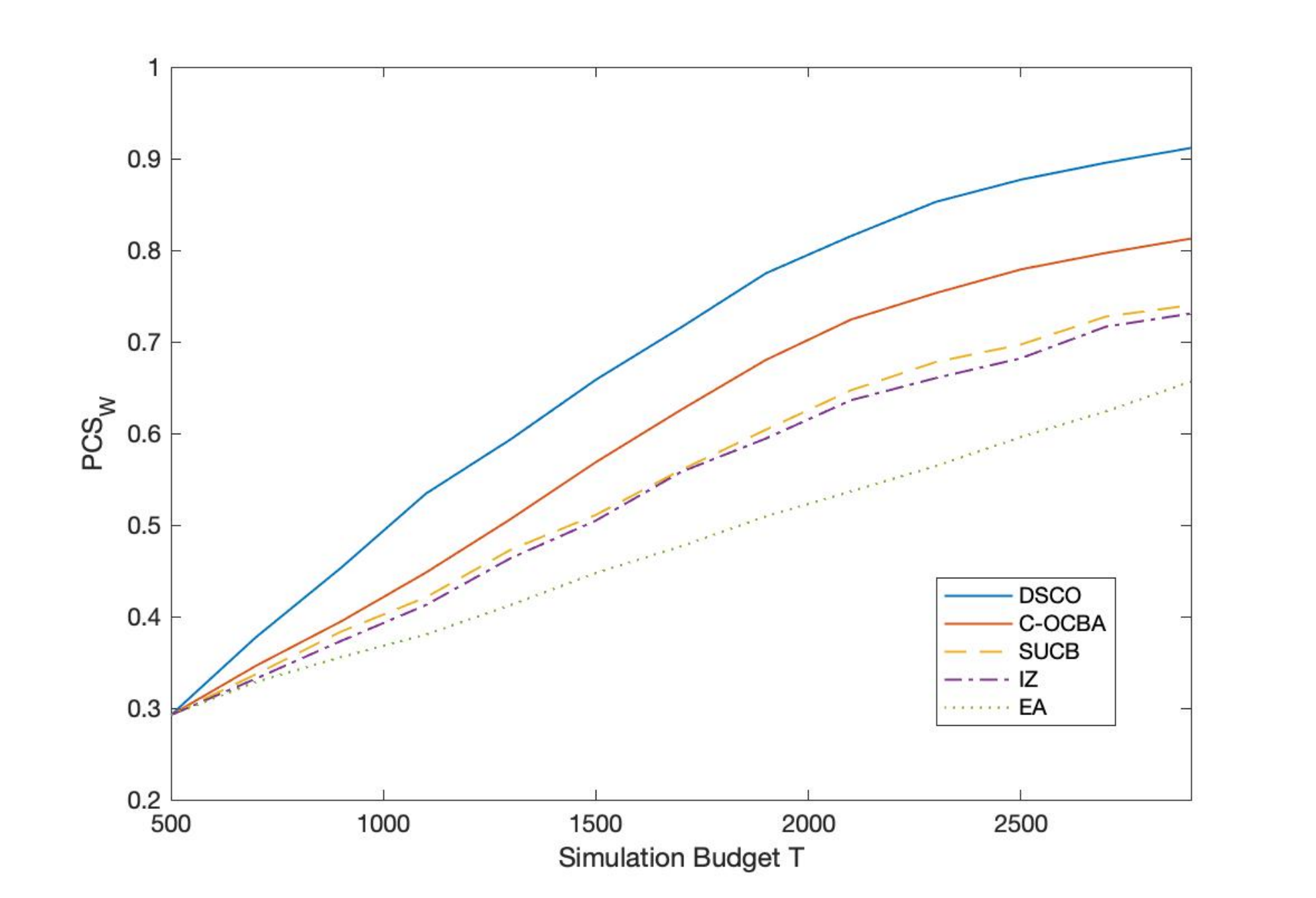
In Figure 6, we can see that DSCO and C-OCBA perform better than IZ, SUCB and EA, which could be attributed to the reason that EA utilizes no sample information, IZ only utilizes sample variances, and SUCB only utilizes sample means while the other two sampling policies utilize the information in the posterior means and variances. In order to attain PCSW=80%\text{PCS}_{\text{W}}=80\%, the number of samples consumed by DSCO is 2000, while EA, IZ, SUCB and C-OCBA require more than 2800 samples. That is to say DSCO reduces the sampling budget by more than 28%. Note that there is no clear performance clustering structure in one cluster case. The performance enhancement of DSCO could be attributed to its stochastic dynamic programming framework which formulates the optimal decision under finite sampling budget. On the contrary, the asymptotically optimal sampling ratio in C-OCBA does not have a theoretical support for the finite-sample performance.
Refer to caption
Figure 6: PCSW\text{PCS}_{\text{W}} of the five sampling policies in one cluster case of Example 1.

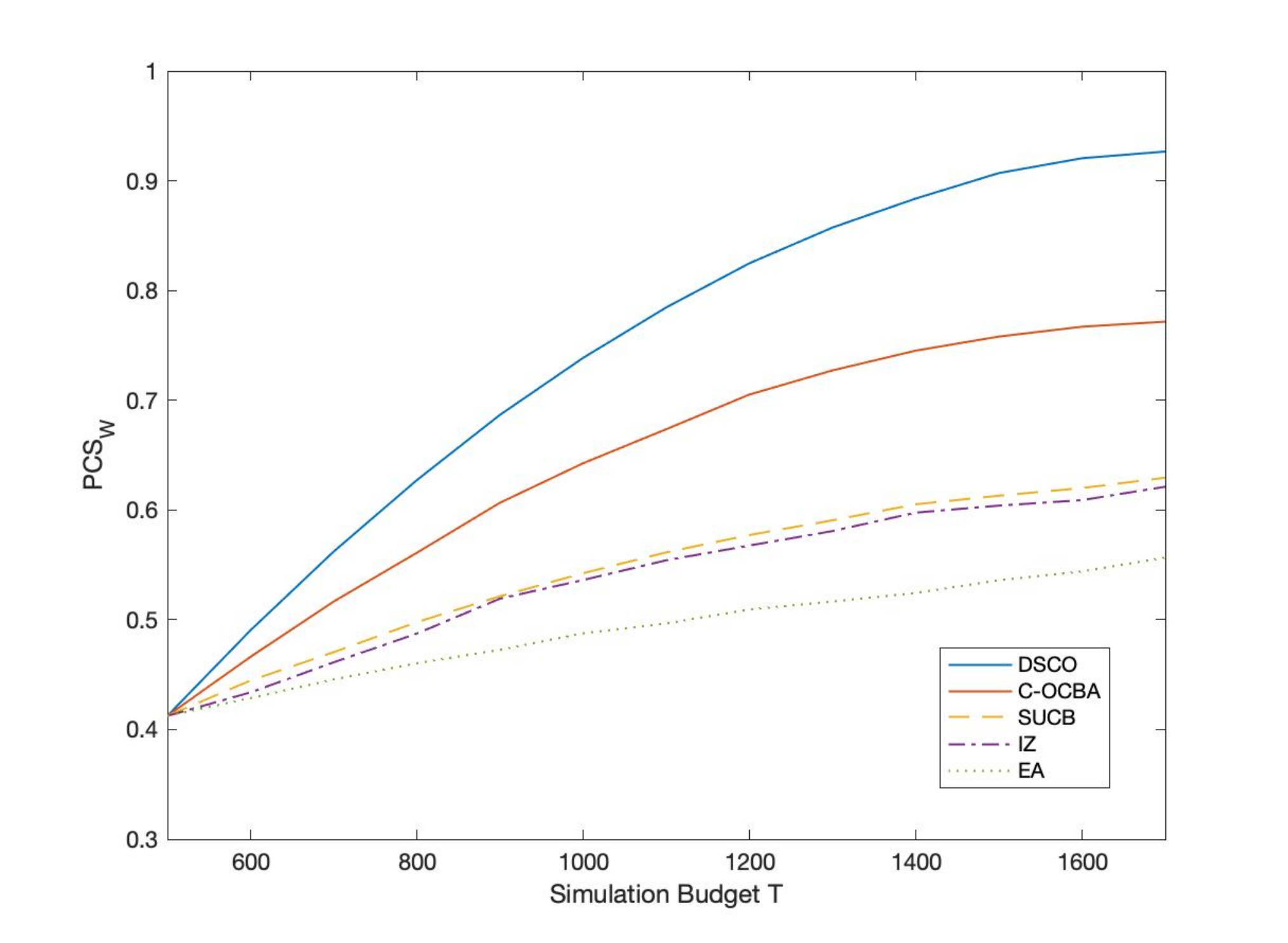
In Figure 7, we can see that DSCO performs significantly better than the other four sampling policies in multiple clusters case. DSCO needs 1400 samples to attain PCSW=90%\text{PCS}_{\text{W}}=90\%, whereas EA, IZ, SUCB and C-OCBA cannot achieve the same PCSW\text{PCS}_{\text{W}} even when simulation budget is 1700. Compared with one cluster case, the advantage of DSCO over C-OCBA increases as performance clustering phenomena becomes apparent. Besides stochastic dynamic programming framework, the performance enhancement of DSCO could be attributed to the benefit of using clustering information which provides useful global information for learning the best designs. DSCO allocates more samples to clusters 2 and 4 where designs have better performances and thus are expected to competitors of the best designs.
Refer to caption
Figure 7: PCSW\text{PCS}_{\text{W}} of the five sampling policies in multiple clusters case of Example 1.

5.1.2 Example 2: 30×3030\times 30 design-context pair

In this example, our proposed DSCO is tested in a larger synthetic case with 30 designs and 30 contexts. In one cluster case, the performances of each design for each context are generated as follows:

yi(𝒙j)∼N(50,152),i=1,…,30,j=1,…,30.\displaystyle y_{i}(\bm{x}_{j})\sim N(50,15^{2}),\ i=1,\ldots,30,\ j=1,\ldots,30.

Context parameters 𝒙j\bm{x}_{j} are set as single-dimensional variables drawn from N⁡(5,12)N(5,1^{2}). As for multiple clusters case, the performances of each design for each context are generated as follows:

yi(𝒙j)∼N(10,1.52),i=1,…,10,j=1,…,10;\displaystyle y_{i}(\bm{x}_{j})\sim N(10,1.5^{2}),\ i=1,\ldots,10,\ j=1,\ldots,10;
yi(𝒙j)∼N(20,1.52),i=11,…,20,j=1,…,10;yi(𝒙j)∼N(30,1.52),i=21,…,30,j=1,…,10;\displaystyle y_{i}(\bm{x}_{j})\sim N(20,1.5^{2}),\ i=11,\ldots,20,\ j=1,\ldots,10;\ y_{i}(\bm{x}_{j})\sim N(30,1.5^{2}),\ i=21,\ldots,30,\ j=1,\ldots,10;
yi(𝒙j)∼N(40,1.52),i=1,…,10,j=11,…,20;yi(𝒙j)∼N(50,1.52),i=11,…,20,j=11,…,20;\displaystyle y_{i}(\bm{x}_{j})\sim N(40,1.5^{2}),\ i=1,\ldots,10,\ j=11,\ldots,20;\ y_{i}(\bm{x}_{j})\sim N(50,1.5^{2}),\ i=11,\ldots,20,\ j=11,\ldots,20;
yi(𝒙j)∼N(60,1.52),i=21,…,30,j=11,…,20;yi(𝒙j)∼N(70,1.52),i=1,…,10,j=21,…,30;\displaystyle y_{i}(\bm{x}_{j})\sim N(60,1.5^{2}),\ i=21,\ldots,30,\ j=11,\ldots,20;\ y_{i}(\bm{x}_{j})\sim N(70,1.5^{2}),\ i=1,\ldots,10,\ j=21,\ldots,30;
yi(𝒙j)∼N(80,1.52),i=11,…,20,j=21,…,30;yi(𝒙j)∼N(90,1.52),i=21,…,30,j=21,…,30.\displaystyle y_{i}(\bm{x}_{j})\sim N(80,1.5^{2}),\ i=11,\ldots,20,\ j=21,\ldots,30;\ y_{i}(\bm{x}_{j})\sim N(90,1.5^{2}),\ i=21,\ldots,30,\ j=21,\ldots,30.

That is to say both design dimension and context dimension have 3 clusters respectively. For design ii and context jj, samples are drawn independently from a normal distribution N⁡(yi​(𝒙j),σi2​(𝒙j))N(y_{i}(\bm{x}_{j}),\sigma_{i}^{2}(\bm{x}_{j})), where σi​(𝒙j)∼U⁡(4,6)\sigma_{i}(\bm{x}_{j})\sim U(4,6). Considering the linear dependency assumption in IZ and SUCB, we set context parameters 𝒙j\bm{x}_{j} as single-dimensional variables generated as follows:

𝒙j∼N(2,12),j=1,…,10;𝒙j∼N(5,12),j=11,…,20;𝒙j∼N(8,12),j=21,…,30.\displaystyle\bm{x}_{j}\sim N(2,1^{2}),\ j=1,\ldots,10;\ \bm{x}_{j}\sim N(5,1^{2}),\ j=11,\ldots,20;\ \bm{x}_{j}\sim N(8,1^{2}),\ j=21,\ldots,30.

The other parameters (n0,δ,h,γn_{0},\delta,h,\gamma) are the same as the last one. The numbers of clusters (KK and LL) are determined based on these initial replications, and the performance clustering phenomenon can been seen in Figure 13 and Figure 14.

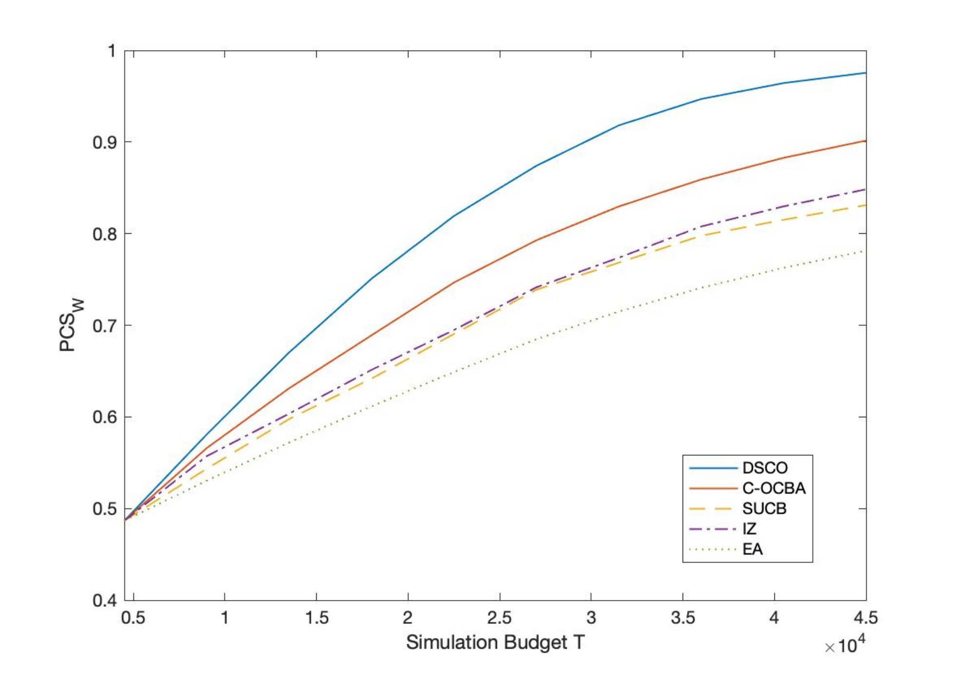
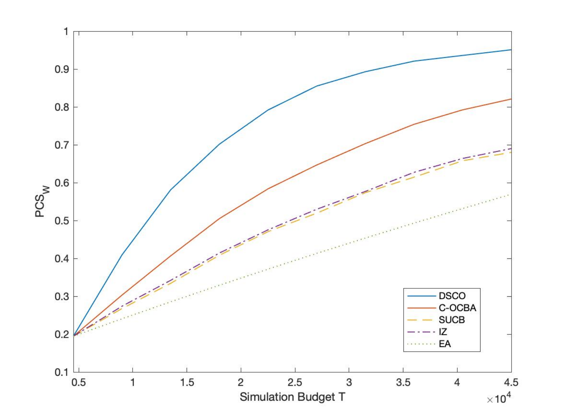
Figures 8 and 9 illustrate the performance of the five sampling policies. Similar to Example 1, DSCO remains as the most efficient sampling policy among the five, and C-OCBA is better than EA, IZ, and SUCB. However, it can be noticed that the advantage of DSCO is more significant when the scale of the problem (the number of designs, contexts, and clusters) grows large. In order to attain PCSW=90%\text{PCS}_{\text{W}}=90\% in one cluster case, DSCO consumes less than 30,000 samples, while EA, IZ, SUCB and C-OCBA require more than 45,000 samples. That is to say DSCO reduces the sampling budget by more than 33%. In multiple clusters case, DSCO needs 33,000 samples to attain PCSW=90%\text{PCS}_{\text{W}}=90\%, whereas EA, IZ, SUCB and C-OCBA cannot achieve the same PCSW\text{PCS}_{\text{W}} even when simulation budget is 45,000. DSCO allocates more samples to clusters 3, 6, and 9 where designs have better performances and thus are expected to competitors of the best designs.
Refer to caption
Figure 8: PCSW\text{PCS}_{\text{W}} of the five sampling policies in one cluster case of Example 2.
Refer to caption
Figure 9: PCSW\text{PCS}_{\text{W}} of the five sampling policies in multiple clusters case of Example 2.

5.2 Cancer Prevention Treatment Example

Non-steroidal anti-inflammatory drugs such as aspirin and statin can prevent the progression of Barrett’s esophagus (BE) to adenocarcinoma, which is a main sub-type of esophageal cancer. However, use of such drugs is associated with numerous potential complications, including gastrointestinal bleeding and hemorrhagic strokes. In this example, we use a Markov chain as shown in Figure 1 to capture the state transition in cancer prevention. Inputs of the simulation model contain design parameters (drug dosages) and context parameters (patient’s characteristics), and some transition probabilities are dependent on these inputs, e.g., red colored transitions in Figure 1 are context-dependent. For patients clustered by certain characteristic, we aim to determine the optimal drug dosage for their cancer prevention treatment. This example has also been considered in Shen et al. 2017 and Gao et al. 2019. Parameters in the probability transition matrix are set based on Hur et al. 2004 and Choi et al. 2014.

Refer to caption
Figure 10: State of the Markov chain.11 1 (1) The transitions from each state to death, which is due to all-cause mortality, are omitted in this illustration. (2) The time duration between state transitions is one month. (3) The details of the transition probabilities depends on whether aspirin chemoprevention or statin chemoprevention is used.

Drug can reduce the probability of canceration, i.e., in Figure 1, the transition probability from state 1 to 4 is less than that from state 3 to 4. Then we denote α=P1,4/P3,4\alpha=P_{1,4}/P_{3,4} as the drug effect. However, drug can also cause complication, and complication rate β\beta is defined as the transition probability from state 1 to 2 in Figure 1. Different drug dosages have different drug effects and complication rates, and their relationship is set as follows:

αaspirin\displaystyle\alpha_{\text{aspirin}} =\displaystyle= 0.5+(a−75)×0.003−(b−120)×0.005,a∈[50,150],b∈[110,150],\displaystyle 0.5+(a-75)\times 0.003-(b-120)\times 0.005,\ a\in[50,150],\ b\in[110,150],
βaspirin\displaystyle\beta_{\text{aspirin}} =\displaystyle= 0.025+(a−75)×0.0005−(b−120)×0.001,a∈[50,150],b∈[110,150],\displaystyle 0.025+(a-75)\times 0.0005-(b-120)\times 0.001,\ a\in[50,150],\ b\in[110,150],
αstatin\displaystyle\alpha_{\text{statin}} =\displaystyle= 0.5+(a−9)×0.0417−(b−120)×0.0025,a∈[6,18],b∈[110,150],\displaystyle 0.5+(a-9)\times 0.0417-(b-120)\times 0.0025,\ a\in[6,18],\ b\in[110,150],
βstatin\displaystyle\beta_{\text{statin}} =\displaystyle= 0.04+(a−9)×0.01+(b−120)×0.001,a∈[6,18],b∈[110,150],\displaystyle 0.04+(a-9)\times 0.01+(b-120)\times 0.001,\ a\in[6,18],\ b\in[110,150],

where aa is drug dosage (mg) and bb is systolic blood pressure (mmHg). In the above formula, based on Hur et al. 2004, we set the standard α\alpha and β\beta of aspirin as 0.5 and 0.025 under standard dosage a=75a=75mg and normal pressure b=120b=120mmHg, and set the standard α\alpha and β\beta of statin as 0.5 and 0.04 under standard dosage a=9a=9mg and normal pressure b=120b=120mmHg. Other coefficients in the above formula are determined by linear regression and (linearly interpolating) few observations already available in the literature. In this example, we consider 40 feasible candidate treatment strategies (designs). Half of them use aspirin, and their dosages are set to be {52.5,57.5,…,142.5,147.5}\{52.5,57.5,\ldots,142.5,147.5\}; the other half use statin, and theirs dosages are set to be {6.2,6.8,…,17.0,17.6}\{6.2,6.8,\ldots,17.0,17.6\}.

Patients’ characteristics are denoted by (x1,x2x_{1},x_{2}), where x1∈[45,80]x_{1}\in[45,80] is the starting age of a treatment and x2∈[110,150]x_{2}\in[110,150] is systolic blood pressure. All-cause mortality λ\lambda denotes the transition probability from each state to death, which is age-related and set as

λ=112×(85−x1).\lambda=\frac{1}{12\times(85-x_{1})}.

This formula is derived from a geometric distribution and a life expectancy of 85 years. Eligibility for resection determines the transitions from state 4 to state 5 or 6, which is affected by x1x_{1} as follows:

P4,5=(1−λ)×[1−(x1−45)×0.00225].P_{4,5}=(1-\lambda)\times[1-(x_{1}-45)\times 0.00225].

The coefficients in the above formula are determined by the results of Hur et al. 2004, stating that 100% of patients at age 45 are eligible for resection while only 91.9% of patients at age 81 are eligible. In general, an older age has a lower eligibility for resection and a higher death rate from all-cause mortality. As for x2x_{2}, it will affect drug effect and complication rate as bb in the expressions of α\alpha and β\beta. We expect to find some clusters in patients’ characteristics. We take 60 possible values of (x1,x2x_{1},x_{2}) as contexts of interest. The performance of a treatment strategy is measured by quality-adjusted life years,

yi​(𝒙j)=limN→+∞​𝔼​[∑t=1NQt​(ai,𝒙j)],y_{i}(\bm{x}_{j})=\underset{N\to+\infty}{\lim}\mathbb{E}[\sum_{t=1}^{N}Q_{t}(a_{i},\bm{x}_{j})],

where Qt​(⋅)Q_{t}(\cdot) is the quality of life at time period tt. The quality of life Qt​(⋅)Q_{t}(\cdot) takes 1 as the initial value, then will have a 50% discount after the development into cancer and a 3% extra discount after surgery, and takes 0 for death. The initial number of simulation replications n0n_{0} is set to be 10. The other parameters involved in IZ are specified as follows: δ=0.2\delta=0.2 and the constant hh is computed when the target PCSW\text{PCS}_{\text{W}} is 95%. The tuning parameter γ\gamma in SUCB is set as 1.

After conducting DSCO, we obtain 4 clusters of designs and 6 clusters of contexts by the posterior probabilities of clustering z^\widehat{z} and v^\widehat{v}. Tables 1 and 2 summarize common statistics (mean and standard deviation) of drug dosage, age, and blood pressure in each cluster. As shown in Table 1, each design cluster only contains one type of drug, that is, DSCO can distinguish different drugs. Treatment strategies using the same drug are classified by DSCO into two levels of dosage. As shown in Table 2, DSCO classifies all contexts into three clusters of age and two clusters of blood pressure. Specifically, Context Clusters 1 and 2 contain the age group of fifties, Context Clusters 3 and 4 contain the age group of sixties, and Context Clusters 5 and 6 contain the age group of seventies; Context Clusters 1, 3, and 5 contain patients with normal blood pressure while Context Clusters 2, 4, and 6 contain patients with hypertension.

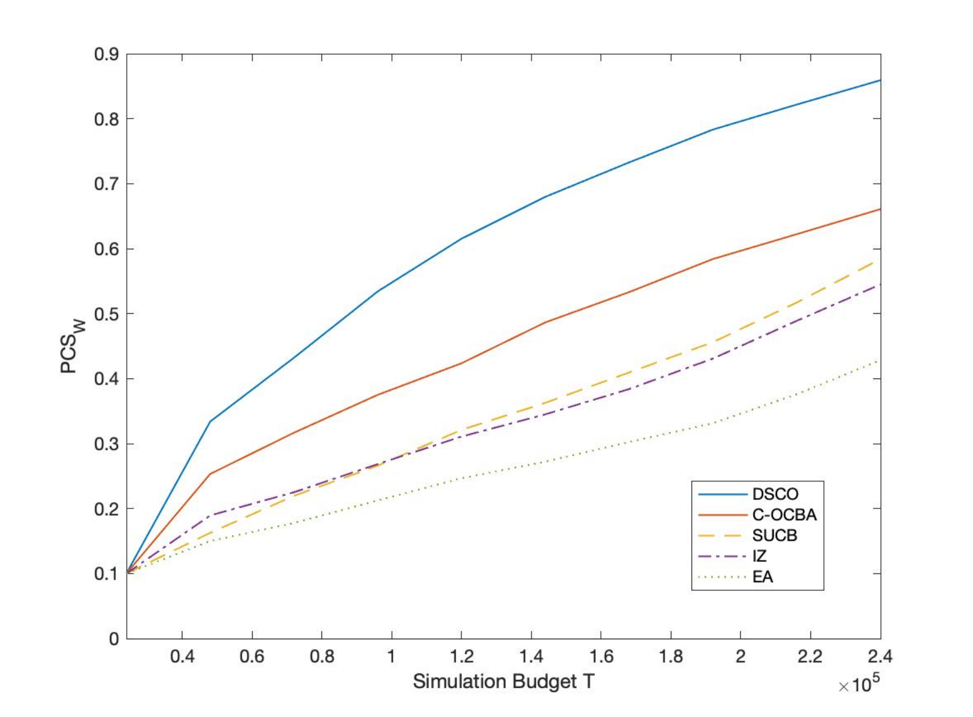
DSCO allocates more samples to design-context pairs in Design Cluster 1 (relatively-high-dose aspirin) and Context Clusters 2, 4, and 6 (hypertension) where designs have better performances, which is in accord with the fact that aspirin significantly reduces major cardiovascular events with the greatest benefit seen in all myocardial infarction (Hansson et al. 1998). The performance comparison is shown in Figure 11. DSCO outperforms EA, IZ, SUCB and C-OCBA. The relative performances of the five compared sampling procedures are similar to those in the two synthetic cases.
Refer to caption
Figure 11: PCSW\text{PCS}_{\text{W}} of the five sampling policies for cancer prevention treatment.

6 Conclusions

This paper studies a sample allocation problem for context-dependent R&S. We take the performance cluster information into consideration, and utilize a Gaussian mixture model as a priori. Under a Bayesian framework, we update model parameters and posterior estimates, and formulate the sequential sampling decision as a stochastic dynamic programming problem. We propose an efficient sampling policy named DSCO, which simultaneously learns the global clustering information and local performance information in design-context pairs. The proposed sampling policy is proved to be consistent and achieve the asymptotically optimal sampling ratio. Numerical experiments demonstrate that DSCO can significantly enhance the efficiency for learning the best designs in all contexts by using performance cluster information.

Acknowledgments.
This work was supported in part by the National Science Foundation of China (NSFC) under Grants 71901003 and 72022001, by the National Science Foundation under Awards ECCS-1462409, CMMI-1462787, CAREER CMMI-1834710 and IIS-1849280, and by the scholarship from China Scholarship Council (CSC) under the Grant CSC. A preliminary version of this work has been published in Proceedings of 2020 Winter Simulation Conference (Li et al. 2020).

References

  • Allesiardo et al. (2014) Allesiardo R, Féraud R, Bouneffouf D (2014) A neural networks committee for the contextual bandit problem. International Conference on Neural Information Processing, 374–381 (Springer).
  • Auer (2000) Auer P (2000) Using upper confidence bounds for online learning. Proceedings 41st Annual Symposium on Foundations of Computer Science, 270–279 (IEEE).
  • Ben-Tal et al. (2009) Ben-Tal A, El Ghaoui L, Nemirovski A (2009) Robust optimization, volume 28 (Princeton University Press).
  • Bertsekas (1995) Bertsekas DP (1995) Dynamic programming and optimal control, volume 1 (Athena scientific Belmont, MA).
  • Bertsimas et al. (2011) Bertsimas D, Brown DB, Caramanis C (2011) Theory and applications of robust optimization. SIAM review 53(3):464–501.
  • Bubeck et al. (2012) Bubeck S, Cesa-Bianchi N, et al. (2012) Regret analysis of stochastic and nonstochastic multi-armed bandit problems. Foundations and Trends® in Machine Learning 5(1):1–122.
  • Chen et al. (2015) Chen CH, Chick SE, Lee LH, Pujowidianto NA (2015) Ranking and selection: efficient simulation budget allocation. Handbook of Simulation Optimization, 45–80 (Springer).
  • Chen et al. (2000) Chen CH, Lin J, Yücesan E, Chick SE (2000) Simulation budget allocation for further enhancing the efficiency of ordinal optimization. Discrete Event Dynamic Systems 10(3):251–270.
  • Chick and Frazier (2012) Chick SE, Frazier P (2012) Sequential sampling with economics of selection procedures. Management Science 58(3):550–569.
  • Choi et al. (2014) Choi SE, Perzan KE, Tramontano AC, Kong CY, Hur C (2014) Statins and aspirin for chemoprevention in barrett’s esophagus: results of a cost-effectiveness analysis. Cancer Prevention Research 7(3):341–350.
  • Dempster et al. (1977) Dempster AP, Laird NM, Rubin DB (1977) Maximum likelihood from incomplete data via the em algorithm. Journal of the Royal Statistical Society: Series B (Methodological) 39(1):1–22.
  • Faloon and Scherer (2017) Faloon M, Scherer B (2017) Individualization of robo-advice. The Journal of Wealth Management 20(1):30–36.
  • Fan et al. (2020) Fan W, Hong LJ, Zhang X (2020) Distributionally robust selection of the best. Management Science 66(1):190–208.
  • Féraud et al. (2016) Féraud R, Allesiardo R, Urvoy T, Clérot F (2016) Random forest for the contextual bandit problem. Artificial Intelligence and Statistics, 93–101.
  • Fraley and Raftery (2002) Fraley C, Raftery AE (2002) Model-based clustering, discriminant analysis, and density estimation. Journal of the American statistical Association 97(458):611–631.
  • Gao et al. (2017a) Gao S, Chen W, Shi L (2017a) A new budget allocation framework for the expected opportunity cost. Operations Research 65(3):787–803.
  • Gao et al. (2019) Gao S, Du J, Chen CH (2019) Selecting the optimal system design under covariates. Proceedings of the 15th IEEE International Conference on Automation Science and Engineering, 547–552 (IEEE Press).
  • Gao et al. (2017b) Gao S, Xiao H, Zhou E, Chen W (2017b) Robust ranking and selection with optimal computing budget allocation. Automatica 81:30–36.
  • Ghosh and Lam (2019) Ghosh S, Lam H (2019) Robust analysis in stochastic simulation: Computation and performance guarantees. Operations Research 67(1):232–249.
  • Glasserman and Xu (2014) Glasserman P, Xu X (2014) Robust risk measurement and model risk. Quantitative Finance 14(1):29–58.
  • Glynn and Juneja (2004) Glynn P, Juneja S (2004) A large deviations perspective on ordinal optimization. Proceedings of the 36th conference on Winter simulation, 577–585 (Winter Simulation Conference).
  • Han et al. (2020) Han Y, Zhou Z, Zhou Z, Blanchet J, Glynn PW, Ye Y (2020) Sequential batch learning in finite-action linear contextual bandits. arXiv preprint arXiv:2004.06321 .
  • Hansson et al. (1998) Hansson L, Zanchetti A, Carruthers SG, Dahlöf B, Elmfeldt D, Julius S, Ménard J, Rahn KH, Wedel H, Westerling S, et al. (1998) Effects of intensive blood-pressure lowering and low-dose aspirin in patients with hypertension: principal results of the hypertension optimal treatment (hot) randomised trial. The Lancet 351(9118):1755–1762.
  • Hong et al. (2011) Hong TP, Song WP, Chiu CT (2011) Evolutionary composite attribute clustering. 2011 International Conference on Technologies and Applications of Artificial Intelligence, 305–308 (IEEE).
  • Hu et al. (2012) Hu Z, Cao J, Hong LJ (2012) Robust simulation of global warming policies using the dice model. Management science 58(12):2190–2206.
  • Hu and Hong (2013) Hu Z, Hong LJ (2013) Kullback-leibler divergence constrained distributionally robust optimization. Available at Optimization Online .
  • Hu and Hong (2015) Hu Z, Hong LJ (2015) Robust simulation of stochastic systems.
  • Hur et al. (2004) Hur C, Nishioka NS, Gazelle GS (2004) Cost-effectiveness of aspirin chemoprevention for barrett’s esophagus. Journal of the National Cancer Institute 96(4):316–325.
  • Kazerouni and Wein (2019) Kazerouni A, Wein LM (2019) Best arm identification in generalized linear bandits. arXiv preprint arXiv:1905.08224 .
  • Kim et al. (2011) Kim ES, Herbst RS, Wistuba II, Lee JJ, Blumenschein GR, Tsao A, Stewart DJ, Hicks ME, Erasmus J, Gupta S, et al. (2011) The battle trial: personalizing therapy for lung cancer. Cancer discovery 1(1):44–53.
  • Kim and Nelson (2001) Kim SH, Nelson BL (2001) A fully sequential procedure for indifference-zone selection in simulation. ACM Transactions on Modeling and Computer Simulation 11(3):251–273.
  • Kim and Nelson (2006) Kim SH, Nelson BL (2006) Selecting the best system. Handbooks in Operations Research and Management Science 13:501–534.
  • Lam (2016) Lam H (2016) Robust sensitivity analysis for stochastic systems. Mathematics of Operations Research 41(4):1248–1275.
  • Lam (2018) Lam H (2018) Sensitivity to serial dependency of input processes: A robust approach. Management Science 64(3):1311–1327.
  • Li et al. (2020) Li H, Lam H, Liang Z, Peng Y (2020) Context-dependent ranking and selection under a bayesian framework. Proceedings of the 2020 Winter Simulation Conference (IEEE Press).
  • Li et al. (2018) Li X, Zhang X, Zheng Z (2018) Data-driven ranking and selection: high-dimensional covariates and general dependence. Proceedings of the 2018 Winter Simulation Conference, 1933–1944 (IEEE Press).
  • Liu et al. (2009) Liu A, Zhang Y, Li J (2009) Personalized movie recommendation. Proceedings of the 17th ACM international conference on Multimedia, 845–848 (ACM).
  • Luo et al. (2015) Luo J, Hong LJ, Nelson BL, Wu Y (2015) Fully sequential procedures for large-scale ranking-and-selection problems in parallel computing environments. Operations Research 63(5):1177–1194.
  • Peng et al. (2016) Peng Y, Chen CH, Fu MC, Hu JQ (2016) Dynamic sampling allocation and design selection. INFORMS Journal on Computing 28(2):195–208.
  • Peng et al. (2018) Peng Y, Chong EK, Chen CH, Fu MC (2018) Ranking and selection as stochastic control. IEEE Transactions on Automatic Control 63(8):2359–2373.
  • Peng et al. (2019) Peng Y, Xu J, Lee LH, Hu JQ, Chen CH (2019) Efficient simulation sampling allocation using multi-fidelity models. IEEE Transactions on Automatic Control 64(8):3156–3169.
  • Perchet et al. (2013) Perchet V, Rigollet P, et al. (2013) The multi-armed bandit problem with covariates. The Annals of Statistics 41(2):693–721.
  • Rigollet and Zeevi (2010) Rigollet P, Zeevi A (2010) Nonparametric bandits with covariates. COLT 2010 54.
  • Rinott (1978) Rinott Y (1978) On two-stage selection procedures and related probability-inequalities. Communications in Statistics - Theory and Methods 7(8):799–811.
  • Rudin et al. (1964) Rudin W, et al. (1964) Principles of mathematical analysis, volume 3 (McGraw-hill New York).
  • Shen et al. (2017) Shen H, Hong LJ, Zhang X (2017) Ranking and selection with covariates for personalized decision making. arXiv preprint arXiv:1710.02642 .
  • Slivkins (2014) Slivkins A (2014) Contextual bandits with similarity information. The Journal of Machine Learning Research 15(1):2533–2568.
  • Soare et al. (2014) Soare M, Lazaric A, Munos R (2014) Best-arm identification in linear bandits. Advances in Neural Information Processing Systems, 828–836.
  • Xu et al. (2018) Xu L, Honda J, Sugiyama M (2018) A fully adaptive algorithm for pure exploration in linear bandits. International Conference on Artificial Intelligence and Statistics, 843–851 (PMLR).
\ECSwitch
\ECHead

Proofs and Supplementary Materials

7 Proof of Theorem 3.1

Proof 7.1

Proof of Theorem 3.1 The log-likelihood of the complete state variables has the following form:

log⁡ℒ⁡(ℰt,𝒚,Z,V,θ)\displaystyle\log\mathcal{L}(\mathcal{E}_{t},\bm{y},Z,V;\theta) (30)
=\displaystyle= (∑i=1n∑k=1Kzi,klogτk)+(∑j=1m∑ℓ=1Lvj,ℓlogωℓ)+∑i=1n∑j=1m{−∑h=1ti​j[12log(2πσi2(𝒙j))+(Yi,h​(𝒙j)−yi​(𝒙j))22​σi2​(𝒙j)]\displaystyle\left(\sum_{i=1}^{n}\sum_{k=1}^{K}z_{i,k}\log\tau_{k}\right)+\left(\sum_{j=1}^{m}\sum_{\ell=1}^{L}v_{j,\ell}\log\omega_{\ell}\right)+\sum_{i=1}^{n}\sum_{j=1}^{m}\left\{-\sum_{h=1}^{t_{ij}}\left[\frac{1}{2}\log(2\pi\sigma_{i}^{2}(\bm{x}_{j}))+\frac{(Y_{i,h}(\bm{x}_{j})-y_{i}(\bm{x}_{j}))^{2}}{2\sigma_{i}^{2}(\bm{x}_{j})}\right]\right.
−∑k=1K∑ℓ=1L[12zi,kvj,ℓlog(2πσk​ℓ2)+zi,kvj,ℓ(yi​(𝒙j)−μk​ℓ)22​σk​ℓ2]}.\displaystyle\left.-\sum_{k=1}^{K}\sum_{\ell=1}^{L}\left[\frac{1}{2}z_{i,k}v_{j,\ell}\log(2\pi\sigma_{k\ell}^{2})+z_{i,k}v_{j,\ell}\frac{(y_{i}(\bm{x}_{j})-\mu_{k\ell})^{2}}{2\sigma_{k\ell}^{2}}\right]\right\}.

Given θ^(t,s)\widehat{\theta}^{(t,s)}, an analytical form for the likelihood of the observations can be obtained by integrating out 𝐲\bm{y}, ZZ, and VV as follow:

ℒ⁡(ℰt,θ^(t,s))\displaystyle\mathcal{L}(\mathcal{E}_{t};\widehat{\theta}^{(t,s)})
=\displaystyle= ∑k1:n∈𝒦∑ℓ1:m∈ℒ(∏i=1nτ^ki(t,s))(∏j=1mω^ℓj(t,s))∏i=1n∏j=1m[∫ℝϕ(yi(𝒙j)|μ^ki​ℓj(t,s),(σ^ki​ℓj2)(t,s))∏h=1ti​jϕ(Yi,h(𝒙j)|yi(𝒙j),σi2(𝒙j))dyi(𝒙j)]\displaystyle\sum_{k_{1:n}\in\mathcal{K}}\sum_{\ell_{1:m}\in\mathcal{L}}\left(\prod_{i=1}^{n}\widehat{\tau}_{k_{i}}^{(t,s)}\right)\left(\prod_{j=1}^{m}\widehat{\omega}_{\ell_{j}}^{(t,s)}\right)\prod_{i=1}^{n}\prod_{j=1}^{m}\left[\int_{\mathbb{R}}\phi\left(y_{i}(\bm{x}_{j})|\widehat{\mu}_{k_{i}\ell_{j}}^{(t,s)},(\widehat{\sigma}_{k_{i}\ell_{j}}^{2})^{(t,s)}\right)\prod_{h=1}^{t_{ij}}\phi\left(Y_{i,h}(\bm{x}_{j})|y_{i}(\bm{x}_{j}),\sigma_{i}^{2}(\bm{x}_{j})\right)dy_{i}(\bm{x}_{j})\right]
=\displaystyle= ∑k1:n∈𝒦∑ℓ1:m∈ℒ(∏i=1nτ^ki(t,s))(∏j=1mω^ℓj(t,s))∏i=1n∏j=1m[12​π​(σ^ki​ℓj2)(t,s)∏h=1ti​j12​π​σi2​(𝒙j)∫ℝexp{−12[(yi​(𝒙j)−μ^ki​ℓj(t,s))2(σ^ki​ℓj2)(t,s)\displaystyle\sum_{k_{1:n}\in\mathcal{K}}\sum_{\ell_{1:m}\in\mathcal{L}}\left(\prod_{i=1}^{n}\widehat{\tau}_{k_{i}}^{(t,s)}\right)\left(\prod_{j=1}^{m}\widehat{\omega}_{\ell_{j}}^{(t,s)}\right)\prod_{i=1}^{n}\prod_{j=1}^{m}\left[\frac{1}{\sqrt{2\pi(\widehat{\sigma}_{k_{i}\ell_{j}}^{2})^{(t,s)}}}\prod_{h=1}^{t_{ij}}\frac{1}{\sqrt{2\pi\sigma_{i}^{2}(\bm{x}_{j})}}\int_{\mathbb{R}}\exp\left\{-\frac{1}{2}\left[\frac{(y_{i}(\bm{x}_{j})-\widehat{\mu}_{k_{i}\ell_{j}}^{(t,s)})^{2}}{(\widehat{\sigma}_{k_{i}\ell_{j}}^{2})^{(t,s)}}\right.\right.\right.
+∑h=1ti​j(Yi,h​(𝒙j)−yi​(𝒙j))2σi2​(𝒙j)]}dyi(𝒙j)]\displaystyle\left.\left.\left.+\sum_{h=1}^{t_{ij}}\frac{(Y_{i,h}(\bm{x}_{j})-y_{i}(\bm{x}_{j}))^{2}}{\sigma_{i}^{2}(\bm{x}_{j})}\right]\right\}dy_{i}(\bm{x}_{j})\right]
=\displaystyle= ∑k1:n∈𝒦∑ℓ1:m∈ℒ(∏i=1nτ^ki(t,s))(∏j=1mω^ℓj(t,s))∏i=1n∏j=1m[Ci​j,ki​ℓj(t,s)∫ℝϕ(yi(𝒙j)|μi​j,ki​ℓj(t,s),(σi​j,ki​ℓj2)(t,s))dyi(𝒙j)]\displaystyle\sum_{k_{1:n}\in\mathcal{K}}\sum_{\ell_{1:m}\in\mathcal{L}}\left(\prod_{i=1}^{n}\widehat{\tau}_{k_{i}}^{(t,s)}\right)\left(\prod_{j=1}^{m}\widehat{\omega}_{\ell_{j}}^{(t,s)}\right)\prod_{i=1}^{n}\prod_{j=1}^{m}\left[C_{ij,k_{i}\ell_{j}}^{(t,s)}\int_{\mathbb{R}}\phi(y_{i}(\bm{x}_{j})|\mu_{ij,k_{i}\ell_{j}}^{(t,s)},(\sigma_{ij,k_{i}\ell_{j}}^{2})^{(t,s)})dy_{i}(\bm{x}_{j})\right]
=\displaystyle= ∑k1:n∈𝒦∑ℓ1:m∈ℒ(∏i=1nτ^ki(t,s))(∏j=1mω^ℓj(t,s))∏i=1n∏j=1mCi​j,ki​ℓj(t,s),\displaystyle\sum_{k_{1:n}\in\mathcal{K}}\sum_{\ell_{1:m}\in\mathcal{L}}\left(\prod_{i=1}^{n}\widehat{\tau}_{k_{i}}^{(t,s)}\right)\left(\prod_{j=1}^{m}\widehat{\omega}_{\ell_{j}}^{(t,s)}\right)\prod_{i=1}^{n}\prod_{j=1}^{m}C_{ij,k_{i}\ell_{j}}^{(t,s)},

where

(σi​j,ki​ℓj2)(t,s)=1/[ti​jσi2​(𝒙j)+1(σ^ki​ℓj2)(t,s)],(\sigma_{ij,k_{i}\ell_{j}}^{2})^{(t,s)}=1\Big/\left[\frac{t_{ij}}{\sigma_{i}^{2}(\bm{x}_{j})}+\frac{1}{(\widehat{\sigma}_{k_{i}\ell_{j}}^{2})^{(t,s)}}\right],
μi​j,ki​ℓj(t,s)=(σi​j,ki​ℓj2)(t,s)​[∑h=1ti​jYi,h​(𝒙j)σi2​(𝒙j)+μ^ki​ℓj(t,s)(σ^ki​ℓj2)(t,s)],\mu_{ij,k_{i}\ell_{j}}^{(t,s)}=(\sigma_{ij,k_{i}\ell_{j}}^{2})^{(t,s)}\left[\frac{\sum_{h=1}^{t_{ij}}Y_{i,h}(\bm{x}_{j})}{\sigma_{i}^{2}(\bm{x}_{j})}+\frac{\widehat{\mu}_{k_{i}\ell_{j}}^{(t,s)}}{(\widehat{\sigma}_{k_{i}\ell_{j}}^{2})^{(t,s)}}\right],

and

Ci​j,ki​ℓj(t,s)=(12​π​σi2​(𝒙j))ti​j2​(σi​j,ki​ℓj2)(t,s)(σ^ki​ℓj2)(t,s)​exp⁡{12​[(μi​j,ki​ℓj(t,s))2(σi​j,ki​ℓj2)(t,s)−∑h=1ti​jYi,h2​(𝒙j)σi2​(𝒙j)−(μ^ki​ℓj(t,s))2(σ^ki​ℓj2)(t,s)]}.C_{ij,k_{i}\ell_{j}}^{(t,s)}=\left(\frac{1}{2\pi\sigma_{i}^{2}(\bm{x}_{j})}\right)^{\frac{t_{ij}}{2}}\sqrt{\frac{(\sigma_{ij,k_{i}\ell_{j}}^{2})^{(t,s)}}{(\widehat{\sigma}_{k_{i}\ell_{j}}^{2})^{(t,s)}}}\exp\left\{\frac{1}{2}\left[\frac{(\mu_{ij,k_{i}\ell_{j}}^{(t,s)})^{2}}{(\sigma_{ij,k_{i}\ell_{j}}^{2})^{(t,s)}}-\frac{\sum_{h=1}^{t_{ij}}Y_{i,h}^{2}(\bm{x}_{j})}{\sigma_{i}^{2}(\bm{x}_{j})}-\frac{(\widehat{\mu}_{k_{i}\ell_{j}}^{(t,s)})^{2}}{(\widehat{\sigma}_{k_{i}\ell_{j}}^{2})^{(t,s)}}\right]\right\}.

By the Bayes’ rule, the posterior distribution of {zi,k=1}\{z_{i,k}=1\} conditional on ℰt\mathcal{E}_{t} and given θ^(t,s)\widehat{\theta}^{(t,s)} is

z^i,k(t,s)=∑k1:n∈𝒦,ki=k∑ℓ1:m∈ℒ(∏i=1nτ^ki(t,s))(∏j=1mω^ℓj(t,s))∏i=1n∏j=1mCi​j,ki​ℓj(t,s)∑k1:n∈𝒦∑ℓ1:m∈ℒ(∏i=1nτ^ki(t,s))(∏j=1mω^ℓj(t,s))∏i=1n∏j=1mCi​j,ki​ℓj(t,s),\widehat{z}_{i,k}^{(t,s)}=\frac{\sum_{k_{1:n}\in\mathcal{K},k_{i}=k}\sum_{\ell_{1:m}\in\mathcal{L}}\left(\prod_{i=1}^{n}\widehat{\tau}_{k_{i}}^{(t,s)}\right)\left(\prod_{j=1}^{m}\widehat{\omega}_{\ell_{j}}^{(t,s)}\right)\prod_{i=1}^{n}\prod_{j=1}^{m}C_{ij,k_{i}\ell_{j}}^{(t,s)}}{\sum_{k_{1:n}\in\mathcal{K}}\sum_{\ell_{1:m}\in\mathcal{L}}\left(\prod_{i=1}^{n}\widehat{\tau}_{k_{i}}^{(t,s)}\right)\left(\prod_{j=1}^{m}\widehat{\omega}_{\ell_{j}}^{(t,s)}\right)\prod_{i=1}^{n}\prod_{j=1}^{m}C_{ij,k_{i}\ell_{j}}^{(t,s)}},

the posterior distribution of {vj,ℓ=1}\{v_{j,\ell}=1\} conditional on ℰt\mathcal{E}_{t} and given θ^(t,s)\widehat{\theta}^{(t,s)} is

v^j,ℓ(t,s)=∑k1:n∈𝒦∑ℓ1:m∈ℒ,ℓj=ℓ(∏i=1nτ^ki(t,s))(∏j=1mω^ℓj(t,s))∏i=1n∏j=1mCi​j,ki​ℓj(t,s)∑k1:n∈𝒦∑ℓ1:m∈ℒ(∏i=1nτ^ki(t,s))(∏j=1mω^ℓj(t,s))∏i=1n∏j=1mCi​j,ki​ℓj(t,s),\widehat{v}_{j,\ell}^{(t,s)}=\frac{\sum_{k_{1:n}\in\mathcal{K}}\sum_{\ell_{1:m}\in\mathcal{L},\ell_{j}=\ell}\left(\prod_{i=1}^{n}\widehat{\tau}_{k_{i}}^{(t,s)}\right)\left(\prod_{j=1}^{m}\widehat{\omega}_{\ell_{j}}^{(t,s)}\right)\prod_{i=1}^{n}\prod_{j=1}^{m}C_{ij,k_{i}\ell_{j}}^{(t,s)}}{\sum_{k_{1:n}\in\mathcal{K}}\sum_{\ell_{1:m}\in\mathcal{L}}\left(\prod_{i=1}^{n}\widehat{\tau}_{k_{i}}^{(t,s)}\right)\left(\prod_{j=1}^{m}\widehat{\omega}_{\ell_{j}}^{(t,s)}\right)\prod_{i=1}^{n}\prod_{j=1}^{m}C_{ij,k_{i}\ell_{j}}^{(t,s)}},

and given θ^(t,s)\widehat{\theta}^{(t,s)}, the posterior distribution of yi​(𝐱j)y_{i}(\bm{x}_{j}) conditional on {zi,k=1}\{z_{i,k}=1\}, {vj,ℓ=1}\{v_{j,\ell}=1\}, and ℰt\mathcal{E}_{t} is

ϕ⁡(yi​(𝒙j)|μi​j,k​ℓ(t,s),(σi​j,k​ℓ2)(t,s)).\phi(y_{i}(\bm{x}_{j})|\mu_{ij,k\ell}^{(t,s)},(\sigma_{ij,k\ell}^{2})^{(t,s)}).

From the log-likelihood of complete state variables given by (30), we have

𝒬⁡(θ|θ^(t,s))\displaystyle\mathcal{Q}(\theta|\widehat{\theta}^{(t,s)})
=\displaystyle= 𝔼[logℒ(ℰt,𝒚,Z,V;θ)|ℰt,θ^(t,s)]\displaystyle\mathbb{E}\left[\log\mathcal{L}(\mathcal{E}_{t},\bm{y},Z,V;\theta)|\mathcal{E}_{t},\widehat{\theta}^{(t,s)}\right]
=\displaystyle= 𝔼[(∑i=1n∑k=1Kzi,klogτk)+(∑j=1m∑ℓ=1Lvj,ℓlogωℓ)−∑i=1n∑j=1m∑k=1K∑ℓ=1L[12zi,kvj,ℓlog(2πσk​ℓ2)\displaystyle\mathbb{E}\left[\left(\sum_{i=1}^{n}\sum_{k=1}^{K}z_{i,k}\log\tau_{k}\right)+\left(\sum_{j=1}^{m}\sum_{\ell=1}^{L}v_{j,\ell}\log\omega_{\ell}\right)-\sum_{i=1}^{n}\sum_{j=1}^{m}\sum_{k=1}^{K}\sum_{\ell=1}^{L}\left[\frac{1}{2}z_{i,k}v_{j,\ell}\log(2\pi\sigma_{k\ell}^{2})\right.\right.
+zi,kvj,ℓ(yi​(𝒙j)−μk​ℓ)22​σk​ℓ2]|ℰt,θ^(t,s)]+C(t,s),\displaystyle\left.\left.+z_{i,k}v_{j,\ell}\frac{(y_{i}(\bm{x}_{j})-\mu_{k\ell})^{2}}{2\sigma_{k\ell}^{2}}\right]\Bigg|\mathcal{E}_{t},\widehat{\theta}^{(t,s)}\right]+C^{(t,s)},

where C(t,s)C^{(t,s)} is a constant independent of θ\theta. The estimate τ^k(t,s+1)\widehat{\tau}_{k}^{(t,s+1)} in the (s+1s+1)-th iteration of the EM algorithm is obtained by solving the following optimization problem:

max𝜏​∑i=1n∑k=1Kz^i,k(t,s)​log⁡τk,s.t.​∑k=1Kτk=1,τk≥0,\underset{\tau}{\max}\sum_{i=1}^{n}\sum_{k=1}^{K}\widehat{z}_{i,k}^{(t,s)}\log\tau_{k},\ \text{s.t.}\sum_{k=1}^{K}\tau_{k}=1,\ \tau_{k}\geq 0,

which is given by

τ^k(t,s+1)=∑i=1nz^i,k(t,s)n.\widehat{\tau}_{k}^{(t,s+1)}=\frac{\sum_{i=1}^{n}\widehat{z}_{i,k}^{(t,s)}}{n}.

Similarly,

ω^ℓ(t,s+1)=∑j=1mv^j,ℓ(t,s)m.\widehat{\omega}_{\ell}^{(t,s+1)}=\frac{\sum_{j=1}^{m}\widehat{v}_{j,\ell}^{(t,s)}}{m}.

Posterior estimate μ^k​ℓ(t,s+1)\widehat{\mu}_{k\ell}^{(t,s+1)} is the solution of the follow equation:

𝔼[∑i=1n∑j=1mzi,kvj,ℓ(yi(𝒙j)−μk​ℓ)|ℰt,θ^(t,s)]=∑i=1n∑j=1mz^i,k(t,s)v^j,ℓ(t,s)𝔼[yi(𝒙j)−μk​ℓ|zi,k=1,vj,ℓ=1,ℰt,θ^(t,s)]=0,\mathbb{E}\left[\sum_{i=1}^{n}\sum_{j=1}^{m}z_{i,k}v_{j,\ell}(y_{i}(\bm{x}_{j})-\mu_{k\ell})\Bigg|\mathcal{E}_{t},\widehat{\theta}^{(t,s)}\right]=\sum_{i=1}^{n}\sum_{j=1}^{m}\widehat{z}_{i,k}^{(t,s)}\widehat{v}_{j,\ell}^{(t,s)}\mathbb{E}\left[y_{i}(\bm{x}_{j})-\mu_{k\ell}\Big|z_{i,k}=1,v_{j,\ell}=1,\mathcal{E}_{t},\widehat{\theta}^{(t,s)}\right]=0,

which yields

μ^k​ℓ(t,s+1)=∑i=1n∑j=1mz^i,k(t,s)​v^j,ℓ(t,s)​μi​j,k​ℓ(t,s)∑i=1n∑j=1mz^i,k(t,s)​v^j,ℓ(t,s).\widehat{\mu}_{k\ell}^{(t,s+1)}=\frac{\sum_{i=1}^{n}\sum_{j=1}^{m}\widehat{z}_{i,k}^{(t,s)}\widehat{v}_{j,\ell}^{(t,s)}\mu_{ij,k\ell}^{(t,s)}}{\sum_{i=1}^{n}\sum_{j=1}^{m}\widehat{z}_{i,k}^{(t,s)}\widehat{v}_{j,\ell}^{(t,s)}}.

To calculate (σ^k​ℓ2)(t,s+1)(\widehat{\sigma}_{k\ell}^{2})^{(t,s+1)}, we solve the follow equation:

∑i=1n∑j=1mz^i,k(t,s)v^j,ℓ(t,s)𝔼[1−(yi​(𝒙j)−μ^k​ℓ(t,s+1))2σk​ℓ2|zi,k=1,vj,ℓ=1,ℰt,θ^(t,s)]=0,\displaystyle\sum_{i=1}^{n}\sum_{j=1}^{m}\widehat{z}_{i,k}^{(t,s)}\widehat{v}_{j,\ell}^{(t,s)}\mathbb{E}\left[1-\frac{(y_{i}(\bm{x}_{j})-\widehat{\mu}_{k\ell}^{(t,s+1)})^{2}}{\sigma_{k\ell}^{2}}\Bigg|z_{i,k}=1,v_{j,\ell}=1,\mathcal{E}_{t},\widehat{\theta}^{(t,s)}\right]=0,

which leads to

(σ^k​ℓ2)(t,s+1)=∑i=1n∑j=1mz^i,k(t,s)​v^j,ℓ(t,s)​[(σi​j,k​ℓ2)(t,s)+(μi​j,k​ℓ(t,s)−μ^k​ℓ(t,s+1))2]∑i=1n∑j=1mz^i,k(t,s)​v^j,ℓ(t,s).(\widehat{\sigma}_{k\ell}^{2})^{(t,s+1)}=\frac{\sum_{i=1}^{n}\sum_{j=1}^{m}\widehat{z}_{i,k}^{(t,s)}\widehat{v}_{j,\ell}^{(t,s)}\left[(\sigma_{ij,k\ell}^{2})^{(t,s)}+\left(\mu_{ij,k\ell}^{(t,s)}-\widehat{\mu}_{k\ell}^{(t,s+1)}\right)^{2}\right]}{\sum_{i=1}^{n}\sum_{j=1}^{m}\widehat{z}_{i,k}^{(t,s)}\widehat{v}_{j,\ell}^{(t,s)}}.

□\square

8 The asymptotic analysis of Theorem 3.1

Proposition 8.1

The posterior probability of {zi,k=1}\{z_{i,k}=1\} conditional on 𝐲\bm{y} and given θ^(s)\widehat{\theta}^{(s)} is

z^i,k(s)=∑k1:n∈𝒦,ki=k∑ℓ1:m∈ℒfτ(s)(k1:n)fω(s)(ℓ1:m)f𝒚(s)(k1:n,ℓ1:m)∑k1:n∈𝒦∑ℓ1:m∈ℒfτ(s)(k1:n)fω(s)(ℓ1:m)f𝒚(s)(k1:n,ℓ1:m),\widehat{z}_{i,k}^{(s)}=\frac{\sum_{k_{1:n}\in\mathcal{K},k_{i}=k}\sum_{\ell_{1:m}\in\mathcal{L}}f_{\tau}^{(s)}(k_{1:n})f_{\omega}^{(s)}(\ell_{1:m})f_{\bm{y}}^{(s)}(k_{1:n},\ell_{1:m})}{\sum_{k_{1:n}\in\mathcal{K}}\sum_{\ell_{1:m}\in\mathcal{L}}f_{\tau}^{(s)}(k_{1:n})f_{\omega}^{(s)}(\ell_{1:m})f_{\bm{y}}^{(s)}(k_{1:n},\ell_{1:m})},

the posterior probability of {vj,ℓ=1}\{v_{j,\ell}=1\} conditional on 𝐲\bm{y} and given θ^(s)\widehat{\theta}^{(s)} is

v^j,ℓ(s)=∑k1:n∈𝒦∑ℓ1:m∈ℒ,ℓj=ℓfτ(s)(k1:n)fω(s)(ℓ1:m)f𝒚(s)(k1:n,ℓ1:m)∑k1:n∈𝒦∑ℓ1:m∈ℒfτ(s)(k1:n)fω(s)(ℓ1:m)f𝒚(s)(k1:n,ℓ1:m),\widehat{v}_{j,\ell}^{(s)}=\frac{\sum_{k_{1:n}\in\mathcal{K}}\sum_{\ell_{1:m}\in\mathcal{L},\ell_{j}=\ell}f_{\tau}^{(s)}(k_{1:n})f_{\omega}^{(s)}(\ell_{1:m})f_{\bm{y}}^{(s)}(k_{1:n},\ell_{1:m})}{\sum_{k_{1:n}\in\mathcal{K}}\sum_{\ell_{1:m}\in\mathcal{L}}f_{\tau}^{(s)}(k_{1:n})f_{\omega}^{(s)}(\ell_{1:m})f_{\bm{y}}^{(s)}(k_{1:n},\ell_{1:m})},

where fτ(s)(k1:n)≜∏i=1nτ^ki(s)f_{\tau}^{(s)}(k_{1:n})\triangleq\prod_{i=1}^{n}\widehat{\tau}_{k_{i}}^{(s)}, fω(s)(ℓ1:m)≜∏j=1mω^ℓj(s)f_{\omega}^{(s)}(\ell_{1:m})\triangleq\prod_{j=1}^{m}\widehat{\omega}_{\ell_{j}}^{(s)}, and f𝐲(s)(k1:n,ℓ1:m)≜∏i=1n∏j=1mϕ(yi(𝐱j)|μ^ki​ℓj(s),(σ^ki​ℓj2)(s))f_{\bm{y}}^{(s)}(k_{1:n},\ell_{1:m})\triangleq\prod_{i=1}^{n}\prod_{j=1}^{m}\phi\left(y_{i}(\bm{x}_{j})|\widehat{\mu}_{k_{i}\ell_{j}}^{(s)},(\widehat{\sigma}_{k_{i}\ell_{j}}^{2})^{(s)}\right). The estimates of the parameters in the (s+1)(s+1)-th iteration of the EM algorithm are given by

τ^k(s+1)=∑i=1nz^i,k(s)n,ω^ℓ(s+1)=∑j=1mv^j,ℓ(s)m,\widehat{\tau}_{k}^{(s+1)}=\frac{\sum_{i=1}^{n}\widehat{z}_{i,k}^{(s)}}{n},\ \widehat{\omega}_{\ell}^{(s+1)}=\frac{\sum_{j=1}^{m}\widehat{v}_{j,\ell}^{(s)}}{m},
μ^k​ℓ(s+1)=∑i=1n∑j=1mz^i,k(s)​v^j,ℓ(s)​yi​(𝒙j)∑i=1n∑j=1mz^i,k(s)​v^j,ℓ(s),\widehat{\mu}_{k\ell}^{(s+1)}=\frac{\sum_{i=1}^{n}\sum_{j=1}^{m}\widehat{z}_{i,k}^{(s)}\widehat{v}_{j,\ell}^{(s)}y_{i}(\bm{x}_{j})}{\sum_{i=1}^{n}\sum_{j=1}^{m}\widehat{z}_{i,k}^{(s)}\widehat{v}_{j,\ell}^{(s)}},

and

(σ^k​ℓ2)(s+1)=∑i=1n∑j=1mz^i,k(s)​v^j,ℓ(s)​(yi​(𝒙j)−μ^k​ℓ(s+1))2∑i=1n∑j=1mz^i,k(s)​v^j,ℓ(s).(\widehat{\sigma}_{k\ell}^{2})^{(s+1)}=\frac{\sum_{i=1}^{n}\sum_{j=1}^{m}\widehat{z}_{i,k}^{(s)}\widehat{v}_{j,\ell}^{(s)}\left(y_{i}(\bm{x}_{j})-\widehat{\mu}_{k\ell}^{(s+1)}\right)^{2}}{\sum_{i=1}^{n}\sum_{j=1}^{m}\widehat{z}_{i,k}^{(s)}\widehat{v}_{j,\ell}^{(s)}}.
Proposition 8.2

Suppose each design-context pair is sampled infinitely often as tt goes to infinity. Then

limt→+∞​[Ci​j,ki​ℓj(t,s)Ci​j,k​ℓ(t,s)−ϕ⁡(yi​(𝒙j)|μ^ki​ℓj(s),(σ^ki​ℓj2)(s))ϕ⁡(yi​(𝒙j)|μ^k​ℓ(s),(σ^k​ℓ2)(s))]=0,a.s.\underset{t\to+\infty}{\lim}\left[\frac{C_{ij,k_{i}\ell_{j}}^{(t,s)}}{C_{ij,k\ell}^{(t,s)}}-\frac{\phi\left(y_{i}(\bm{x}_{j})|\widehat{\mu}_{k_{i}\ell_{j}}^{(s)},(\widehat{\sigma}_{k_{i}\ell_{j}}^{2})^{(s)}\right)}{\phi\left(y_{i}(\bm{x}_{j})|\widehat{\mu}_{k\ell}^{(s)},(\widehat{\sigma}_{k\ell}^{2})^{(s)}\right)}\right]=0,\ a.s.

where

Ci​j,k​ℓ(t,s)≜(12​π​σi2​(𝒙j))ti​j2​(σi​j,k​ℓ2)(t,s)(σ^k​ℓ2)(t,s)​exp⁡{12​[(μi​j,k​ℓ(t,s))2(σi​j,k​ℓ2)(t,s)−∑h=1ti​jYi,h2​(𝒙j)σi2​(𝒙j)−(μ^k​ℓ(t,s))2(σ^k​ℓ2)(t,s)]}.C_{ij,k\ell}^{(t,s)}\triangleq\left(\frac{1}{2\pi\sigma_{i}^{2}(\bm{x}_{j})}\right)^{\frac{t_{ij}}{2}}\sqrt{\frac{(\sigma_{ij,k\ell}^{2})^{(t,s)}}{(\widehat{\sigma}_{k\ell}^{2})^{(t,s)}}}\exp\left\{\frac{1}{2}\left[\frac{(\mu_{ij,k\ell}^{(t,s)})^{2}}{(\sigma_{ij,k\ell}^{2})^{(t,s)}}-\frac{\sum_{h=1}^{t_{ij}}Y_{i,h}^{2}(\bm{x}_{j})}{\sigma_{i}^{2}(\bm{x}_{j})}-\frac{(\widehat{\mu}_{k\ell}^{(t,s)})^{2}}{(\widehat{\sigma}_{k\ell}^{2})^{(t,s)}}\right]\right\}.
Proof 8.3

Proof of Proposition 8.2 We have

(μi​j,ki​ℓj(t,s))2(σi​j,ki​ℓj2)(t,s)\displaystyle\frac{(\mu_{ij,k_{i}\ell_{j}}^{(t,s)})^{2}}{(\sigma_{ij,k_{i}\ell_{j}}^{2})^{(t,s)}}
=\displaystyle= (σi​j,ki​ℓj2)(t,s)​[∑h=1ti​jYi,h​(𝒙j)σi2​(𝒙j)+μ^ki​ℓj(t,s)(σ^ki​ℓj2)(t,s)]2\displaystyle(\sigma_{ij,k_{i}\ell_{j}}^{2})^{(t,s)}\left[\frac{\sum_{h=1}^{t_{ij}}Y_{i,h}(\bm{x}_{j})}{\sigma_{i}^{2}(\bm{x}_{j})}+\frac{\widehat{\mu}_{k_{i}\ell_{j}}^{(t,s)}}{(\widehat{\sigma}_{k_{i}\ell_{j}}^{2})^{(t,s)}}\right]^{2}
=\displaystyle= ti​j​[1ti​j​∑h=1ti​jYi,h​(𝒙j)]2σi2​(𝒙j)−[1ti​j​∑h=1ti​jYi,h​(𝒙j)]2(σ^ki​ℓj2)(t,s)+2​[1ti​j​∑h=1ti​jYi,h​(𝒙j)]​μ^ki​ℓj(t,s)(σ^ki​ℓj2)(t,s)+oa.s.​(1),\displaystyle\frac{t_{ij}\left[\frac{1}{t_{ij}}\sum_{h=1}^{t_{ij}}Y_{i,h}(\bm{x}_{j})\right]^{2}}{\sigma_{i}^{2}(\bm{x}_{j})}-\frac{\left[\frac{1}{t_{ij}}\sum_{h=1}^{t_{ij}}Y_{i,h}(\bm{x}_{j})\right]^{2}}{(\widehat{\sigma}_{k_{i}\ell_{j}}^{2})^{(t,s)}}+2\frac{\left[\frac{1}{t_{ij}}\sum_{h=1}^{t_{ij}}Y_{i,h}(\bm{x}_{j})\right]\widehat{\mu}_{k_{i}\ell_{j}}^{(t,s)}}{(\widehat{\sigma}_{k_{i}\ell_{j}}^{2})^{(t,s)}}+o_{a.s.}(1),

where oa.s.​(1)o_{a.s.}(1) means a term that goes to zero as tt goes to infinity a.s., by observing limt→+∞​ti​j​(σi​j,ki​ℓj2)(t,s)=σi2​(𝐱j)\underset{t\to+\infty}{\lim}t_{ij}(\sigma_{ij,k_{i}\ell_{j}}^{2})^{(t,s)}=\sigma_{i}^{2}(\bm{x}_{j}), a.s. Therefore, the conclusion of the proposition can be obtained straightforwardly by observing limt→+∞​1ti​j​∑h=1ti​jYi,h​(𝐱j)=yi​(𝐱j)\underset{t\to+\infty}{\lim}\frac{1}{t_{ij}}\sum_{h=1}^{t_{ij}}Y_{i,h}(\bm{x}_{j})=y_{i}(\bm{x}_{j}), a.s., and canceling the terms independent of kik_{i} and ℓj\ell_{j} in Ci​j,ki​ℓj(t,s)C_{ij,k_{i}\ell_{j}}^{(t,s)}. □\square

The above proposition implies Ci​j,ki​ℓj(t,s)C_{ij,k_{i}\ell_{j}}^{(t,s)} corresponds to ϕ⁡(yi​(𝒙j)|μ^ki​ℓj(s),(σ^ki​ℓj2)(s))\phi\left(y_{i}(\bm{x}_{j})|\widehat{\mu}_{k_{i}\ell_{j}}^{(s)},(\widehat{\sigma}_{k_{i}\ell_{j}}^{2})^{(s)}\right). Further, fY(t,s)(ℰt|k1:n,ℓ1:m)f_{Y}^{(t,s)}(\mathcal{E}_{t}|k_{1:n},\ell_{1:m}) corresponds to f𝒚(s)(k1:n,ℓ1:m)f_{\bm{y}}^{(s)}(k_{1:n},\ell_{1:m}) in the classic results. Therefore, Corollary 8.4 is a direct conclusion from Proposition 8.2.

Corollary 8.4

Suppose each design-context pair is sampled infinitely often as tt goes to infinity. Then

limt→+∞​[z^i,k(t,s)−z^i,k(s)]=0​and​limt→+∞​[v^j,ℓ(t,s)−v^j,ℓ(s)]=0,a.s.\underset{t\to+\infty}{\lim}\left[\widehat{z}_{i,k}^{(t,s)}-\widehat{z}_{i,k}^{(s)}\right]=0\ \text{and}\ \underset{t\to+\infty}{\lim}\left[\widehat{v}_{j,\ell}^{(t,s)}-\widehat{v}_{j,\ell}^{(s)}\right]=0,\ a.s.

9 Proposition 9.1

Proposition 9.1

As ti​jt_{ij} goes to infinity, Ci​j,ki​ℓj(t,s)C_{ij,k_{i}\ell_{j}}^{(t,s)} approaches zero when σi2​(xj)≥1/(2​e​π)\sigma_{i}^{2}(x_{j})\geq 1/(2e\pi); otherwise Ci​j,ki​ℓj(t,s)C_{ij,k_{i}\ell_{j}}^{(t,s)} goes to infinity.

Proof 9.2

Proof of Proposition 9.1 Notice that we have limt→+∞​μ^ki​ℓj(t,s)=μki​ℓj(s)​and​limt→+∞​(σ^ki​ℓj2)(t,s)=(σki​ℓj2)(s)>0\underset{t\to+\infty}{\lim}\widehat{\mu}_{k_{i}\ell_{j}}^{(t,s)}=\mu_{k_{i}\ell_{j}}^{(s)}\ \text{and}\ \underset{t\to+\infty}{\lim}(\widehat{\sigma}_{k_{i}\ell_{j}}^{2})^{(t,s)}=(\sigma_{k_{i}\ell_{j}}^{2})^{(s)}>0. Therefore, when 2​e​π​σi2​(xj)≥12e\pi\sigma_{i}^{2}(x_{j})\geq 1,

limti​j→+∞​Ci​j,ki​ℓj(t,s)\displaystyle\underset{t_{ij}\to+\infty}{\lim}C_{ij,k_{i}\ell_{j}}^{(t,s)}
=\displaystyle= limti​j→+∞​(12​π​σi2​(𝒙j))ti​j2​(σi​j,ki​ℓj2)(t,s)(σ^ki​ℓj2)(t,s)​exp⁡{12​[(μi​j,ki​ℓj(t,s))2(σi​j,ki​ℓj2)(t,s)−∑h=1ti​jYi,h2​(𝒙j)σi2​(𝒙j)−(μ^ki​ℓj(t,s))2(σ^ki​ℓj2)(t,s)]}\displaystyle\underset{t_{ij}\to+\infty}{\lim}\left(\frac{1}{2\pi\sigma_{i}^{2}(\bm{x}_{j})}\right)^{\frac{t_{ij}}{2}}\sqrt{\frac{(\sigma_{ij,k_{i}\ell_{j}}^{2})^{(t,s)}}{(\widehat{\sigma}_{k_{i}\ell_{j}}^{2})^{(t,s)}}}\exp\left\{\frac{1}{2}\left[\frac{(\mu_{ij,k_{i}\ell_{j}}^{(t,s)})^{2}}{(\sigma_{ij,k_{i}\ell_{j}}^{2})^{(t,s)}}-\frac{\sum_{h=1}^{t_{ij}}Y_{i,h}^{2}(\bm{x}_{j})}{\sigma_{i}^{2}(\bm{x}_{j})}-\frac{(\widehat{\mu}_{k_{i}\ell_{j}}^{(t,s)})^{2}}{(\widehat{\sigma}_{k_{i}\ell_{j}}^{2})^{(t,s)}}\right]\right\}
=\displaystyle= limti​j→+∞​(12​π​σi2​(𝒙j))ti​j2​σi2​(xj)ti​j​(σki​ℓj2)(s)​exp⁡{12​[ti​j​(E⁡[Yi,h​(𝒙j)])2σi2​(𝒙j)−ti​j​E​[Yi,h2​(𝒙j)]σi2​(𝒙j)−o⁡(ti​j)]}\displaystyle\underset{t_{ij}\to+\infty}{\lim}\left(\frac{1}{2\pi\sigma_{i}^{2}(\bm{x}_{j})}\right)^{\frac{t_{ij}}{2}}\sqrt{\frac{\sigma_{i}^{2}(x_{j})}{t_{ij}(\sigma_{k_{i}\ell_{j}}^{2})^{(s)}}}\exp\left\{\frac{1}{2}\left[\frac{t_{ij}\left(E[Y_{i,h}(\bm{x}_{j})]\right)^{2}}{\sigma_{i}^{2}(\bm{x}_{j})}-\frac{t_{ij}E[Y_{i,h}^{2}(\bm{x}_{j})]}{\sigma_{i}^{2}(\bm{x}_{j})}-o(t_{ij})\right]\right\}
=\displaystyle= limti​j→+∞​(12​π​σi2​(𝒙j))ti​j2​σi2​(xj)ti​j​(σki​ℓj2)(s)​exp⁡{12​[−ti​j−o⁡(ti​j)]}\displaystyle\underset{t_{ij}\to+\infty}{\lim}\left(\frac{1}{2\pi\sigma_{i}^{2}(\bm{x}_{j})}\right)^{\frac{t_{ij}}{2}}\sqrt{\frac{\sigma_{i}^{2}(x_{j})}{t_{ij}(\sigma_{k_{i}\ell_{j}}^{2})^{(s)}}}\exp\left\{\frac{1}{2}\left[-t_{ij}-o(t_{ij})\right]\right\}
=\displaystyle= 0,\displaystyle 0,

where the second equation follows from the law of large numbers and the last equation is a result of 2​e​π​σi2​(xj)≥12e\pi\sigma_{i}^{2}(x_{j})\geq 1. Similarly, when 2​e​π​σi2​(xj)<12e\pi\sigma_{i}^{2}(x_{j})<1, limti​j→+∞​Ci​j,ki​ℓj(t,s)=+∞\underset{t_{ij}\to+\infty}{\lim}C_{ij,k_{i}\ell_{j}}^{(t,s)}=+\infty since the exponential function grows faster than any power function. □\square

10 Algorithm 1

Log transformation: For each k1:n∈𝒦,ℓ1:m∈ℒk_{1:n}\in\mathcal{K},\ell_{1:m}\in\mathcal{L},
logf(t,s)(k1:n,ℓ1:m)≜∑i=1nlogτ^ki(t,s)+∑j=1mlogω^ℓj(t,s)+∑i=1n∑j=1mlogCi​j,ki​ℓj(t,s).\log f^{(t,s)}(k_{1:n},\ell_{1:m})\triangleq\sum_{i=1}^{n}\log\widehat{\tau}_{k_{i}}^{(t,s)}+\sum_{j=1}^{m}\log\widehat{\omega}_{\ell_{j}}^{(t,s)}+\sum_{i=1}^{n}\sum_{j=1}^{m}\log C_{ij,k_{i}\ell_{j}}^{(t,s)}.

Magnification:
g(t,s)(k1:n,ℓ1:m)≜logf(t,s)(k1:n,ℓ1:m)−maxk1:n∈𝒦,ℓ1:m∈ℒlogf(t,s)(k1:n,ℓ1:m).g^{(t,s)}(k_{1:n},\ell_{1:m})\triangleq\log f^{(t,s)}(k_{1:n},\ell_{1:m})-\underset{k_{1:n}\in\mathcal{K},\ell_{1:m}\in\mathcal{L}}{\max}\log f^{(t,s)}(k_{1:n},\ell_{1:m}).

Equivalent transformation:
z^i,k(t,s)=∑k1:n∈𝒦,ki=k∑ℓ1:m∈ℒexp(g(t,s)(k1:n,ℓ1:m))∑k1:n∈𝒦∑ℓ1:m∈ℒexp(g(t,s)(k1:n,ℓ1:m)),\widehat{z}_{i,k}^{(t,s)}=\frac{\sum_{k_{1:n}\in\mathcal{K},k_{i}=k}\sum_{\ell_{1:m}\in\mathcal{L}}\exp(g^{(t,s)}(k_{1:n},\ell_{1:m}))}{\sum_{k_{1:n}\in\mathcal{K}}\sum_{\ell_{1:m}\in\mathcal{L}}\exp(g^{(t,s)}(k_{1:n},\ell_{1:m}))},
v^j,ℓ(t,s)=∑k1:n∈𝒦∑ℓ1:m∈ℒ,ℓj=ℓexp(g(t,s)(k1:n,ℓ1:m))∑k1:n∈𝒦∑ℓ1:m∈ℒexp(g(t,s)(k1:n,ℓ1:m)).\widehat{v}_{j,\ell}^{(t,s)}=\frac{\sum_{k_{1:n}\in\mathcal{K}}\sum_{\ell_{1:m}\in\mathcal{L},\ell_{j}=\ell}\exp(g^{(t,s)}(k_{1:n},\ell_{1:m}))}{\sum_{k_{1:n}\in\mathcal{K}}\sum_{\ell_{1:m}\in\mathcal{L}}\exp(g^{(t,s)}(k_{1:n},\ell_{1:m}))}.

return z^i,k(t,s)\widehat{z}_{i,k}^{(t,s)} and v^j,ℓ(t,s)\widehat{v}_{j,\ell}^{(t,s)}.
Algorithm 1 Equivalent transformation for z^i,k(t,s)\widehat{z}_{i,k}^{(t,s)} and v^j,ℓ(t,s)\widehat{v}_{j,\ell}^{(t,s)}

11 Proposition 11.1

Proposition 11.1

The denominator satisfies

1≤∑k1:n∈𝒦∑ℓ1:m∈ℒexp(g(t,s)(k1:n,ℓ1:m))≤Kn×Lm.1\leq\sum_{k_{1:n}\in\mathcal{K}}\sum_{\ell_{1:m}\in\mathcal{L}}\exp(g^{(t,s)}(k_{1:n},\ell_{1:m}))\leq K^{n}\times L^{m}~.
Proof 11.2

Proof of Proposition 11.1 Note that each g(t,s)(k1:n,ℓ1:m)g^{(t,s)}(k_{1:n},\ell_{1:m}) is not greater than zero, and there must exist a clustering situation (k1:n,ℓ1:m)(k_{1:n},\ell_{1:m}) such that g(t,s)(k1:n,ℓ1:m)=0g^{(t,s)}(k_{1:n},\ell_{1:m})=0. Therefore, the denominator ∑k1:n∈𝒦∑ℓ1:m∈ℒexp(g(t,s)(k1:n,ℓ1:m))\sum_{k_{1:n}\in\mathcal{K}}\sum_{\ell_{1:m}\in\mathcal{L}}\exp(g^{(t,s)}(k_{1:n},\ell_{1:m})) is not less than one and is bounded by Kn×LmK^{n}\times L^{m}.□\square

12 Exponential decay of approximation error

Proposition 12.1

The error between the integral of multivariate standard normal density over a region Ω\Omega and that over the maximal tangent inner ball in Ω\Omega decreases to zero at least in an order of O(t(n−1)/2e−t/2)O(t^{(n-1)/2}e^{-t/2}) as t→+∞t\to+\infty.

Proof 12.2

Proof of Proposition 12.1 We have

∫⋯∫Ω1(2​π)nexp(−12∑i=1nzi2)dz1…dzn−∫⋯∫∑i=1nzi2≤R21(2​π)nexp(−12∑i=1nzi2)dz1…dzn\displaystyle\int\cdots\int_{\Omega}\frac{1}{\sqrt{(2\pi)^{n}}}\exp(-\frac{1}{2}\sum_{i=1}^{n}z_{i}^{2})dz_{1}\ldots dz_{n}-\int\cdots\int_{\sum_{i=1}^{n}z_{i}^{2}\leq R^{2}}\frac{1}{\sqrt{(2\pi)^{n}}}\exp(-\frac{1}{2}\sum_{i=1}^{n}z_{i}^{2})dz_{1}\ldots dz_{n}
≤\displaystyle\leq 1−∫⋯∫∑i=1nzi2≤R21(2​π)nexp(−12∑i=1nzi2)dz1…dzn\displaystyle 1-\int\cdots\int_{\sum_{i=1}^{n}z_{i}^{2}\leq R^{2}}\frac{1}{\sqrt{(2\pi)^{n}}}\exp(-\frac{1}{2}\sum_{i=1}^{n}z_{i}^{2})dz_{1}\ldots dz_{n}
=\displaystyle= ∫R+∞∫0π⋯∫0π∫02​π1(2​π)nexp(−12r2)rn−1(sinφ1)n−2⋯sinφn−2drdφ1…dφn−1\displaystyle\int_{R}^{+\infty}\int_{0}^{\pi}\cdots\int_{0}^{\pi}\int_{0}^{2\pi}\frac{1}{\sqrt{(2\pi)^{n}}}\exp(-\frac{1}{2}r^{2})r^{n-1}(\sin\varphi_{1})^{n-2}\cdots\sin\varphi_{n-2}\ drd\varphi_{1}\ldots d\varphi_{n-1}
=\displaystyle= C⁡(n)​∫R+∞exp⁡(−12​r2)​rn−1​𝑑r\displaystyle C(n)\int_{R}^{+\infty}\exp(-\frac{1}{2}r^{2})r^{n-1}\ dr

where RR is the radius of the inner ball, and

C(n)=1(2​π)n∫0π⋯∫0π∫02​π(sinφ1)n−2⋯sinφn−2dφ1…dφn−1C(n)=\frac{1}{\sqrt{(2\pi)^{n}}}\int_{0}^{\pi}\cdots\int_{0}^{\pi}\int_{0}^{2\pi}(\sin\varphi_{1})^{n-2}\cdots\sin\varphi_{n-2}\ d\varphi_{1}\ldots d\varphi_{n-1}

is a constant depending only on nn.

Given by integration by parts,

∫R+∞exp⁡(−12​r2)​rn−1​𝑑r=1n​([exp⁡(−12​r2)​rn]R+∞−∫R+∞exp⁡(−12​r2)​(−r)​rn−1​𝑑r).\displaystyle\int_{R}^{+\infty}\exp(-\frac{1}{2}r^{2})r^{n-1}\ dr=\frac{1}{n}\left(\left[\exp(-\frac{1}{2}r^{2})r^{n}\right]_{R}^{+\infty}-\int_{R}^{+\infty}\exp(-\frac{1}{2}r^{2})(-r)r^{n-1}\ dr\right).

In addition, we have

∫R+∞exp⁡(−12​r2)​rn​𝑑r≥R​∫R+∞exp⁡(−12​r2)​rn−1​𝑑r.\int_{R}^{+\infty}\exp(-\frac{1}{2}r^{2})r^{n}\ dr\geq R\int_{R}^{+\infty}\exp(-\frac{1}{2}r^{2})r^{n-1}\ dr.

Therefore,

exp⁡(−12​R2)​Rn+n​∫R+∞exp⁡(−12​r2)​rn−1​𝑑r≥R​∫R+∞exp⁡(−12​r2)​rn−1​𝑑r\displaystyle\exp(-\frac{1}{2}R^{2})R^{n}+n\int_{R}^{+\infty}\exp(-\frac{1}{2}r^{2})r^{n-1}\ dr\geq R\int_{R}^{+\infty}\exp(-\frac{1}{2}r^{2})r^{n-1}\ dr

which concludes

∫R+∞exp⁡(−12​r2)​rn−1​𝑑r≤1R−n​exp⁡(−12​R2)​Rn.\int_{R}^{+\infty}\exp(-\frac{1}{2}r^{2})r^{n-1}\ dr\leq\frac{1}{R-n}\exp(-\frac{1}{2}R^{2})R^{n}.

Note that

R2=mini≠1​(μ⟨1⟩j​t​j,k⟨1⟩j​t​ℓj(t)−μ⟨i⟩j​t​j,k⟨i⟩j​t​ℓj(t))2(σ⟨1⟩j​t​j,k⟨1⟩j​t​ℓj2)(t)+(σ⟨i⟩j​t​j,k⟨i⟩j​t​ℓj2)(t)=O⁡(t),R^{2}=\underset{i\neq 1}{\min}\frac{\left(\mu_{\langle 1\rangle_{jt}j,k_{\langle 1\rangle_{jt}}\ell_{j}}^{(t)}-\mu_{\langle i\rangle_{jt}j,k_{\langle i\rangle_{jt}}\ell_{j}}^{(t)}\right)^{2}}{\left(\sigma_{\langle 1\rangle_{jt}j,k_{\langle 1\rangle_{jt}}\ell_{j}}^{2}\right)^{(t)}+\left(\sigma_{\langle i\rangle_{jt}j,k_{\langle i\rangle_{jt}}\ell_{j}}^{2}\right)^{(t)}}=O(t),

which concludes the proposition.□\square

13 Approximations of z^i,k(t;(r,q)E)\widehat{z}_{i,k}^{(t;(r,q)_{E})} and v^j,ℓ(t;(r,q)E)\widehat{v}_{j,\ell}^{(t;(r,q)_{E})}

In order to reduce the complexity of

z^i,k(t;(r,q)E)=∑k1:n∈𝒦,ki=k∑ℓ1:m∈ℒfτ(t;(r,q)E)(k1:n)fω(t;(r,q)E)(ℓ1:m)fY(t;(r,q)E)(ℰt|k1:n,ℓ1:m)∑k1:n∈𝒦∑ℓ1:m∈ℒfτ(t;(r,q)E)(k1:n)fω(t;(r,q)E)(ℓ1:m)fY(t;(r,q)E)(ℰt|k1:n,ℓ1:m),\widehat{z}_{i,k}^{(t;(r,q)_{E})}=\frac{\sum_{k_{1:n}\in\mathcal{K},k_{i}=k}\sum_{\ell_{1:m}\in\mathcal{L}}f_{\tau}^{(t;(r,q)_{E})}(k_{1:n})f_{\omega}^{(t;(r,q)_{E})}(\ell_{1:m})f_{Y}^{(t;(r,q)_{E})}(\mathcal{E}_{t}|k_{1:n},\ell_{1:m})}{\sum_{k_{1:n}\in\mathcal{K}}\sum_{\ell_{1:m}\in\mathcal{L}}f_{\tau}^{(t;(r,q)_{E})}(k_{1:n})f_{\omega}^{(t;(r,q)_{E})}(\ell_{1:m})f_{Y}^{(t;(r,q)_{E})}(\mathcal{E}_{t}|k_{1:n},\ell_{1:m})},

we focus on the change in the numerator of z^i,k(t;(r,q)E)\widehat{z}_{i,k}^{(t;(r,q)_{E})} and make the following approximation by considering the denominators of z^i,k(t;(r,q)E)\widehat{z}_{i,k}^{(t;(r,q)_{E})} and z^i,k(t)\widehat{z}_{i,k}^{(t)} as a same constant:

z^i,k(t;(r,q)E)z^i,k(t)≈∑k1:n∈𝒦,ki=k∑ℓ1:m∈ℒfτ(t;(r,q)E)(k1:n)fω(t;(r,q)E)(ℓ1:m)fY(t;(r,q)E)(ℰt|k1:n,ℓ1:m)∑k1:n∈𝒦,ki=k∑ℓ1:m∈ℒfτ(t)(k1:n)fω(t)(ℓ1:m)fY(t)(ℰt|k1:n,ℓ1:m).\frac{\widehat{z}_{i,k}^{(t;(r,q)_{E})}}{\widehat{z}_{i,k}^{(t)}}\approx\frac{\sum_{k_{1:n}\in\mathcal{K},k_{i}=k}\sum_{\ell_{1:m}\in\mathcal{L}}f_{\tau}^{(t;(r,q)_{E})}(k_{1:n})f_{\omega}^{(t;(r,q)_{E})}(\ell_{1:m})f_{Y}^{(t;(r,q)_{E})}(\mathcal{E}_{t}|k_{1:n},\ell_{1:m})}{\sum_{k_{1:n}\in\mathcal{K},k_{i}=k}\sum_{\ell_{1:m}\in\mathcal{L}}f_{\tau}^{(t)}(k_{1:n})f_{\omega}^{(t)}(\ell_{1:m})f_{Y}^{(t)}(\mathcal{E}_{t}|k_{1:n},\ell_{1:m})}.

Note that ki∗=arg⁡maxk=1,…,K​z^i,k(t)k_{i}^{*}=\underset{k=1,\ldots,K}{\arg\max}\ \widehat{z}_{i,k}^{(t)} and ℓj∗=arg⁡maxℓ=1,…,L​v^j,ℓ(t)\ell_{j}^{*}=\underset{\ell=1,\ldots,L}{\arg\max}\ \widehat{v}_{j,\ell}^{(t)} denote the indexes of the optimal posterior probabilities of clustering for each design and context. If there indeed exists obvious clustering phenomenon in designs and contexts, then we would tend to have ϕ⁡(yi​(𝒙j)|μ^ki∗​ℓj∗(t,s),(σ^ki∗​ℓj∗2)(t,s))≫ϕ⁡(yi​(𝒙j)|μ^k​ℓ(t,s),(σ^k​ℓ2)(t,s)),∀(k,ℓ)≠(ki∗,ℓj∗)\phi\left(y_{i}(\bm{x}_{j})|\widehat{\mu}_{k_{i}^{*}\ell_{j}^{*}}^{(t,s)},(\widehat{\sigma}_{k_{i}^{*}\ell_{j}^{*}}^{2})^{(t,s)}\right)\gg\phi\left(y_{i}(\bm{x}_{j})|\widehat{\mu}_{k\ell}^{(t,s)},(\widehat{\sigma}_{k\ell}^{2})^{(t,s)}\right),\ \forall(k,\ell)\neq(k_{i}^{*},\ell_{j}^{*}). According to the results of Proposition 8.2, we have Ci​j,ki∗​ℓj∗(t,s)≫Ci​j,k​ℓ(t,s)C_{ij,k_{i}^{*}\ell_{j}^{*}}^{(t,s)}\gg C_{ij,k\ell}^{(t,s)} when tt is relatively large. Therefore, by ignoring the events with non-optimal posterior probabilities of clustering, we have

∑k1:n∈𝒦,ki=k∑ℓ1:m∈ℒfτ(t)(k1:n)fω(t)(ℓ1:m)fY(t)(ℰt|k1:n,ℓ1:m)\displaystyle\sum_{k_{1:n}\in\mathcal{K},k_{i}=k}\sum_{\ell_{1:m}\in\mathcal{L}}f_{\tau}^{(t)}(k_{1:n})f_{\omega}^{(t)}(\ell_{1:m})f_{Y}^{(t)}(\mathcal{E}_{t}|k_{1:n},\ell_{1:m})
≈\displaystyle\approx fτ(t)([k1:(i−1)∗,k,k(i+1):n∗])fω(t)(ℓ1:m∗)fY(t)(ℰt|[k1:(i−1)∗,k,k(i+1):n∗],ℓ1:m∗)\displaystyle f_{\tau}^{(t)}([k_{1:(i-1)}^{*},k,k_{(i+1):n}^{*}])f_{\omega}^{(t)}(\ell_{1:m}^{*})f_{Y}^{(t)}(\mathcal{E}_{t}|[k_{1:(i-1)}^{*},k,k_{(i+1):n}^{*}],\ell_{1:m}^{*})
=\displaystyle= τ^k(t)​(∏i′=1,i′≠inτ^ki′∗(t))​(∏j=1mω^ℓj∗(t))​(∏j=1mCi​j,k​ℓj∗(t))​(∏i′=1,i′≠in∏j=1mCi′​j,ki′∗​ℓj∗(t)),\displaystyle\widehat{\tau}_{k}^{(t)}\left(\prod_{i^{\prime}=1,i^{\prime}\neq i}^{n}\widehat{\tau}_{k_{i^{\prime}}^{*}}^{(t)}\right)\left(\prod_{j=1}^{m}\widehat{\omega}_{\ell_{j}^{*}}^{(t)}\right)\left(\prod_{j=1}^{m}C_{ij,k\ell_{j}^{*}}^{(t)}\right)\left(\prod_{i^{\prime}=1,i^{\prime}\neq i}^{n}\prod_{j=1}^{m}C_{i^{\prime}j,k_{i^{\prime}}^{*}\ell_{j}^{*}}^{(t)}\right),

and then

z^i,k(t;(r,q)E)z^i,k(t)≈(∏j=1mCi​j,k​ℓj∗(t;(r,q)E))​(∏i′=1,i′≠in∏j=1mCi′​j,ki′∗​ℓj∗(t;(r,q)E))(∏j=1mCi​j,k​ℓj∗(t))​(∏i′=1,i′≠in∏j=1mCi′​j,ki′∗​ℓj∗(t)).\frac{\widehat{z}_{i,k}^{(t;(r,q)_{E})}}{\widehat{z}_{i,k}^{(t)}}\approx\frac{\left(\prod_{j=1}^{m}C_{ij,k\ell_{j}^{*}}^{(t;(r,q)_{E})}\right)\left(\prod_{i^{\prime}=1,i^{\prime}\neq i}^{n}\prod_{j=1}^{m}C_{i^{\prime}j,k_{i^{\prime}}^{*}\ell_{j}^{*}}^{(t;(r,q)_{E})}\right)}{\left(\prod_{j=1}^{m}C_{ij,k\ell_{j}^{*}}^{(t)}\right)\left(\prod_{i^{\prime}=1,i^{\prime}\neq i}^{n}\prod_{j=1}^{m}C_{i^{\prime}j,k_{i^{\prime}}^{*}\ell_{j}^{*}}^{(t)}\right)}.

The following proposition indicates sampling a design-context pair (r,q)(r,q) would become less likely to change the likelihood of observations for other design-context pair (i,j)(i,j) as the number of samples grows large.

Proposition 13.1

Suppose each design-context pair is sampled infinitely often as t goes to infinity. For each (i,j)≠(r,q)(i,j)\neq(r,q),

limt→+∞​Ci​j,k​ℓ(t;(r,q)E)Ci​j,k​ℓ(t)=1,a.s.\underset{t\to+\infty}{\lim}\dfrac{C_{ij,k\ell}^{(t;(r,q)_{E})}}{C_{ij,k\ell}^{(t)}}=1,\ a.s.
Proof 13.2

Proof of Proposition 13.1 Note that for (i,j)≠(r,q)(i,j)\neq(r,q),

Ci​j,k​ℓ(t;(r,q)E)Ci​j,k​ℓ(t)=(σi​j,k​ℓ2)(t;(r,q)E)(σ^k​ℓ2)(t;(r,q)E)​(σ^k​ℓ2)(t)(σi​j,k​ℓ2)(t)​exp⁡{12​[((μi​j,k​ℓ(t))2(σi​j,k​ℓ2)(t;(r,q)E)−(μi​j,k​ℓ(t))2(σi​j,k​ℓ2)(t))−((μ^k​ℓ(t))2(σ^k​ℓ2)(t;(r,q)E)−(μ^k​ℓ(t))2(σ^k​ℓ2)(t))]}.\displaystyle\dfrac{C_{ij,k\ell}^{(t;(r,q)_{E})}}{C_{ij,k\ell}^{(t)}}=\sqrt{\frac{(\sigma_{ij,k\ell}^{2})^{\left(t;(r,q)_{E}\right)}}{(\widehat{\sigma}_{k\ell}^{2})^{\left(t;(r,q)_{E}\right)}}\frac{(\widehat{\sigma}_{k\ell}^{2})^{(t)}}{(\sigma_{ij,k\ell}^{2})^{(t)}}}\exp\left\{\frac{1}{2}\left[\left(\frac{(\mu_{ij,k\ell}^{(t)})^{2}}{(\sigma_{ij,k\ell}^{2})^{\left(t;(r,q)_{E}\right)}}-\frac{(\mu_{ij,k\ell}^{(t)})^{2}}{(\sigma_{ij,k\ell}^{2})^{\left(t\right)}}\right)-\left(\frac{(\widehat{\mu}_{k\ell}^{(t)})^{2}}{(\widehat{\sigma}_{k\ell}^{2})^{\left(t;(r,q)_{E}\right)}}-\frac{(\widehat{\mu}_{k\ell}^{(t)})^{2}}{(\widehat{\sigma}_{k\ell}^{2})^{\left(t\right)}}\right)\right]\right\}.

In addition,

limt→+∞​1(σi​j,k​ℓ2)(t;(r,q)E)−1(σi​j,k​ℓ2)(t)=limt→+∞​1(σ^k​ℓ2)(t;(r,q)E)−1(σ^k​ℓ2)(t)=0​a.s.\displaystyle\underset{t\to+\infty}{\lim}\frac{1}{(\sigma_{ij,k\ell}^{2})^{\left(t;(r,q)_{E}\right)}}-\frac{1}{(\sigma_{ij,k\ell}^{2})^{\left(t\right)}}=\underset{t\to+\infty}{\lim}\frac{1}{(\widehat{\sigma}_{k\ell}^{2})^{\left(t;(r,q)_{E}\right)}}-\frac{1}{(\widehat{\sigma}_{k\ell}^{2})^{\left(t\right)}}=0\ a.s.

where the first equation is due to (i,j)≠(r,q)(i,j)\neq(r,q) and the second equation is due to that both (σ^k​ℓ2)(t;(r,q)E)(\widehat{\sigma}_{k\ell}^{2})^{\left(t;(r,q)_{E}\right)} and (σ^k​ℓ2)(t)(\widehat{\sigma}_{k\ell}^{2})^{\left(t\right)} converge to a same positive value. Therefore, limt→+∞​Ci​j,k​ℓ(t;(r,q)E)Ci​j,k​ℓ(t)=1​a.s.\underset{t\to+\infty}{\lim}\dfrac{C_{ij,k\ell}^{(t;(r,q)_{E})}}{C_{ij,k\ell}^{(t)}}=1\ a.s. □\square

The proposition suggests us to make the following approximation:

z^r,k(t;(r,q)E)z^r,k(t)≈Cr​q,k​ℓq∗(t;(r,q)E)Cr​q,k​ℓq∗(t)\frac{\widehat{z}_{r,k}^{(t;(r,q)_{E})}}{\widehat{z}_{r,k}^{(t)}}\approx\frac{C_{rq,k\ell_{q}^{*}}^{(t;(r,q)_{E})}}{C_{rq,k\ell_{q}^{*}}^{(t)}}

and

z^i,k(t;(r,q)E)z^i,k(t)≈Cr​q,kr∗​ℓq∗(t;(r,q)E)Cr​q,kr∗​ℓq∗(t),i≠r.\frac{\widehat{z}_{i,k}^{(t;(r,q)_{E})}}{\widehat{z}_{i,k}^{(t)}}\approx\frac{C_{rq,k_{r}^{*}\ell_{q}^{*}}^{(t;(r,q)_{E})}}{C_{rq,k_{r}^{*}\ell_{q}^{*}}^{(t)}},\ i\neq r.

Further, the following proposition provides the asymptotic results for the change rate of the likelihood of observations for design-context pair (r,q)(r,q) after allocating one more sample to this design-context pair.

Proposition 13.3

Suppose each design-context pair is sampled infinitely often as tt goes to infinity. Then

limt→+∞​[Cr​q,k​ℓq∗(t;(r,q)E)Cr​q,k​ℓq∗(t)−12​π​σr2​(𝒙q)​exp⁡{12​[−(μr​q,k​ℓq∗(t)−μ^k​ℓq∗(t))2​(σr​q,k​ℓq∗4)(t)σr2​(𝒙q)​(σ^k​ℓq∗4)(t)]}]=0​a.s.\displaystyle\underset{t\to+\infty}{\lim}\left[\frac{C_{rq,k\ell_{q}^{*}}^{(t;(r,q)_{E})}}{C_{rq,k\ell_{q}^{*}}^{(t)}}-\sqrt{\frac{1}{2\pi\sigma_{r}^{2}(\bm{x}_{q})}}\exp\left\{\frac{1}{2}\left[-\frac{(\mu_{rq,k\ell_{q}^{*}}^{(t)}-\widehat{\mu}_{k\ell_{q}^{*}}^{(t)})^{2}(\sigma_{rq,k\ell_{q}^{*}}^{4})^{(t)}}{\sigma_{r}^{2}(\bm{x}_{q})(\widehat{\sigma}_{k\ell_{q}^{*}}^{4})^{(t)}}\right]\right\}\right]=0\ a.s.
Proof 13.4

Proof of Proposition 13.3 Note that

Cr​q,k​ℓq∗(t;(r,q)E)Cr​q,k​ℓq∗(t)=\displaystyle\dfrac{C_{rq,k\ell_{q}^{*}}^{(t;(r,q)_{E})}}{C_{rq,k\ell_{q}^{*}}^{(t)}}= 12​π​σr2​(𝒙q)(σr​q,k​ℓq∗2)(t;(r,q)E)(σ^k​ℓq∗2)(t;(r,q)E)​(σ^k​ℓq∗2)(t)(σr​q,k​ℓq∗2)(t)exp{12[[∑h=1tr​qYr,h​(𝒙q)+μr​q,k​ℓq∗(t)σr2​(𝒙q)+μ^k​ℓq∗(t)(σ^k​ℓq∗2)(t)]2tr​q+1σr2​(𝒙q)+1(σ^k​ℓq∗2)(t)\displaystyle\sqrt{\frac{1}{2\pi\sigma_{r}^{2}(\bm{x}_{q})}}\sqrt{\frac{(\sigma_{rq,k\ell_{q}^{*}}^{2})^{\left(t;(r,q)_{E}\right)}}{(\widehat{\sigma}_{k\ell_{q}^{*}}^{2})^{\left(t;(r,q)_{E}\right)}}\frac{(\widehat{\sigma}_{k\ell_{q}^{*}}^{2})^{(t)}}{(\sigma_{rq,k\ell_{q}^{*}}^{2})^{(t)}}}\exp\left\{\frac{1}{2}\left[\dfrac{\left[\dfrac{\sum_{h=1}^{t_{rq}}Y_{r,h}(\bm{x}_{q})+\mu_{rq,k\ell_{q}^{*}}^{(t)}}{\sigma_{r}^{2}(\bm{x}_{q})}+\dfrac{\widehat{\mu}_{k\ell_{q}^{*}}^{(t)}}{\left(\widehat{\sigma}_{k\ell_{q}^{*}}^{2}\right)^{(t)}}\right]^{2}}{\dfrac{t_{rq}+1}{\sigma_{r}^{2}(\bm{x}_{q})}+\dfrac{1}{\left(\widehat{\sigma}_{k\ell_{q}^{*}}^{2}\right)^{(t)}}}\right.\right.
−[∑h=1tr​qYr,h​(𝒙q)σr2​(𝒙q)+μ^k​ℓq∗(t)(σ^k​ℓq∗2)(t)]2tr​qσr2​(𝒙q)+1(σ^k​ℓq∗2)(t)−(μr​q,k​ℓq∗(t))2σr2​(𝒙q)]}.\displaystyle\left.\left.-\dfrac{\left[\dfrac{\sum_{h=1}^{t_{rq}}Y_{r,h}(\bm{x}_{q})}{\sigma_{r}^{2}(\bm{x}_{q})}+\dfrac{\widehat{\mu}_{k\ell_{q}^{*}}^{(t)}}{(\widehat{\sigma}_{k\ell_{q}^{*}}^{2})^{(t)}}\right]^{2}}{\dfrac{t_{rq}}{\sigma_{r}^{2}(\bm{x}_{q})}+\dfrac{1}{\left(\widehat{\sigma}_{k\ell_{q}^{*}}^{2}\right)^{(t)}}}-\dfrac{\left(\mu_{rq,k\ell_{q}^{*}}^{(t)}\right)^{2}}{\sigma_{r}^{2}(\bm{x}_{q})}\right]\right\}.

In addition, limt→+∞​(σr​q,k​ℓq∗2)(t;(r,q)E)(σ^k​ℓq∗2)(t;(r,q)E)​(σ^k​ℓq∗2)(t)(σr​q,k​ℓq∗2)(t)=1​a.s.\underset{t\to+\infty}{\lim}\dfrac{(\sigma_{rq,k\ell_{q}^{*}}^{2})^{\left(t;(r,q)_{E}\right)}}{(\widehat{\sigma}_{k\ell_{q}^{*}}^{2})^{\left(t;(r,q)_{E}\right)}}\dfrac{(\widehat{\sigma}_{k\ell_{q}^{*}}^{2})^{(t)}}{(\sigma_{rq,k\ell_{q}^{*}}^{2})^{(t)}}=1\ a.s. and limt→+∞​1tr​q​∑h=1tr​qYr,h​(𝐱q)−μr​q,k​ℓq∗(t)=0​a.s.\underset{t\to+\infty}{\lim}\dfrac{1}{t_{rq}}\sum_{h=1}^{t_{rq}}Y_{r,h}(\bm{x}_{q})-\mu_{rq,k\ell_{q}^{*}}^{(t)}=0\ a.s., which means that the effect of prior information on the posterior estimate vanishes as the number of samples goes to infinity. Therefore, the conclusion of the proposition can be obtained. □\square

Summarizing the discussions above, we have

z^r,k(t;(r,q)E)z^r,k(t)≈12​π​σr2​(𝒙q)​exp⁡{12​[−(μr​q,k​ℓq∗(t)−μ^k​ℓq∗(t))2​(σr​q,k​ℓq∗4)(t)σr2​(𝒙q)​(σ^k​ℓq∗4)(t)]}\displaystyle\frac{\widehat{z}_{r,k}^{(t;(r,q)_{E})}}{\widehat{z}_{r,k}^{(t)}}\approx\sqrt{\frac{1}{2\pi\sigma_{r}^{2}(\bm{x}_{q})}}\exp\left\{\frac{1}{2}\left[-\frac{(\mu_{rq,k\ell_{q}^{*}}^{(t)}-\widehat{\mu}_{k\ell_{q}^{*}}^{(t)})^{2}(\sigma_{rq,k\ell_{q}^{*}}^{4})^{(t)}}{\sigma_{r}^{2}(\bm{x}_{q})(\widehat{\sigma}_{k\ell_{q}^{*}}^{4})^{(t)}}\right]\right\}

and similarly

v^q,ℓ(t;(r,q)E)v^q,ℓ(t)≈12​π​σr2​(𝒙q)​exp⁡{12​[−(μr​q,kr∗​ℓ(t)−μ^kr∗​ℓ(t))2​(σr​q,kr∗​ℓ4)(t)σr2​(𝒙q)​(σ^kr∗​ℓ4)(t)]}.\displaystyle\frac{\widehat{v}_{q,\ell}^{(t;(r,q)_{E})}}{\widehat{v}_{q,\ell}^{(t)}}\approx\sqrt{\frac{1}{2\pi\sigma_{r}^{2}(\bm{x}_{q})}}\exp\left\{\frac{1}{2}\left[-\frac{(\mu_{rq,k_{r}^{*}\ell}^{(t)}-\widehat{\mu}_{k_{r}^{*}\ell}^{(t)})^{2}(\sigma_{rq,k_{r}^{*}\ell}^{4})^{(t)}}{\sigma_{r}^{2}(\bm{x}_{q})(\widehat{\sigma}_{k_{r}^{*}\ell}^{4})^{(t)}}\right]\right\}.

Notice that the formulas on the right-hand side of the approximations can be calculated efficiently. Due to constraints ∑k=1Kz^i,k(t;(r,q)E)=1\sum_{k=1}^{K}\widehat{z}_{i,k}^{(t;(r,q)_{E})}=1 and ∑ℓ=1Lv^j,ℓ(t;(r,q)E)=1\sum_{\ell=1}^{L}\widehat{v}_{j,\ell}^{(t;(r,q)_{E})}=1, we obtain efficient approximations for the one-step-ahead looking posterior probabilities of clustering z^i,k(t;(r,q)E)\widehat{z}_{i,k}^{(t;(r,q)_{E})} and v^j,ℓ(t;(r,q)E)\widehat{v}_{j,\ell}^{(t;(r,q)_{E})} by normalization as shown in (4.1.1) and (4.1.1).

14 Algorithm 2

Inputs: Number of designs nn, number of contexts mm, total sampling budget TT, common initial sample size n0n_{0}.
Generate n0n_{0} samples from each design ii in each context jj, and t←n×m×n0t\leftarrow n\times m\times n_{0}.
Determine number of design clusters KK and number of context clusters LL by BIC (1) and EM algorithm (2)-(3).
Initialize parameter estimates τ^k(t)\widehat{\tau}_{k}^{(t)}, ω^ℓ(t)\widehat{\omega}_{\ell}^{(t)}, μ^k​ℓ(t)\widehat{\mu}_{k\ell}^{(t)}, (σ^k​ℓ2)(t)(\widehat{\sigma}_{k\ell}^{2})^{(t)}, and posterior estimates z^i,k(t)\widehat{z}_{i,k}^{(t)}, v^j,ℓ(t)\widehat{v}_{j,\ell}^{(t)}, μ^i​j,k​ℓ(t)\widehat{\mu}_{ij,k\ell}^{(t)}, (σ^i​j,k​ℓ2)(t)(\widehat{\sigma}_{ij,k\ell}^{2})^{(t)} by Theorem 3.1 (4)-(10).
while t≤Tt\leq T do
if there exists a (r,qr,q) such that V⁡(ℰt,(r,q))>V⁡(ℰt)V(\mathcal{E}_{t};(r,q))>V(\mathcal{E}_{t}) then
     Choose At+1​(ℰt)={(r∗,q∗)|V⁡(ℰt,(r∗,q∗))=max(r,q)​V​(ℰt,(r,q))}A_{t+1}(\mathcal{E}_{t})=\left\{(r^{*},q^{*})\Bigg|V(\mathcal{E}_{t};(r^{*},q^{*}))=\underset{(r,q)}{\max}\ V(\mathcal{E}_{t};(r,q))\right\}, where (σi​j,ki​ℓj2)(t,(r,q)E)(\sigma^{2}_{ij,k_{i}\ell_{j}})^{(t,(r,q)_{E})}, (σ^k​ℓ2)(t,(r,q)E)(\widehat{\sigma}^{2}_{k\ell})^{(t,(r,q)_{E})}, z^i,k(t,(r,q)E)\widehat{z}_{i,k}^{(t,(r,q)_{E})}, and v^j,ℓ(t,(r,q)E)\widehat{v}_{j,\ell}^{(t,(r,q)_{E})} are calculated by (4.1)-(4.1.1) and V⁡(ℰt,(r,q))V(\mathcal{E}_{t};(r,q)) is calculated by (21).
Take a sample Yr∗,tr∗​q∗+1​(𝒙q∗)Y_{r^{*},t_{r^{*}q^{*}}+1}(\bm{x}_{q^{*}}) from design r∗r^{*} in context q∗q^{*}.
Update parameter estimates τ^k(t)\widehat{\tau}_{k}^{(t)}, ω^ℓ(t)\widehat{\omega}_{\ell}^{(t)}, μ^k​ℓ(t)\widehat{\mu}_{k\ell}^{(t)}, (σ^k​ℓ2)(t)(\widehat{\sigma}_{k\ell}^{2})^{(t)}, and posterior estimates z^i,k(t)\widehat{z}_{i,k}^{(t)}, v^j,ℓ(t)\widehat{v}_{j,\ell}^{(t)}, μ^i​j,k​ℓ(t)\widehat{\mu}_{ij,k\ell}^{(t)}, (σ^i​j,k​ℓ2)(t)(\widehat{\sigma}_{ij,k\ell}^{2})^{(t)} by Theorem 3.1 (4)-(10).
Set t←t+1t\leftarrow t+1. else
     while W⁡(ℰt,(r∗,q∗))>V⁡(ℰt)W(\mathcal{E}_{t};(r^{*},q^{*}))>V(\mathcal{E}_{t}) and t≤Tt\leq T do
         Choose At+1​(ℰt)={(r∗,q∗)|W⁡(ℰt,(r∗,q∗))=max(r,q)​W​(ℰt,(r,q))}A_{t+1}(\mathcal{E}_{t})=\left\{(r^{*},q^{*})\Bigg|W(\mathcal{E}_{t};(r^{*},q^{*}))=\underset{(r,q)}{\max}\ W(\mathcal{E}_{t};(r,q))\right\}, where (σi​j,ki​ℓj2)(t,(r,q)E)(\sigma^{2}_{ij,k_{i}\ell_{j}})^{(t,(r,q)_{E})} and (σ^k​ℓ2)(t,(r,q)E)(\widehat{\sigma}^{2}_{k\ell})^{(t,(r,q)_{E})} are calculated by (4.1)-(16) and W⁡(ℰt,(r,q))W(\mathcal{E}_{t};(r,q)) is calculated by (24).
Take a sample Yr∗,tr∗​q∗+1​(𝒙q∗)Y_{r^{*},t_{r^{*}q^{*}}+1}(\bm{x}_{q^{*}}) from design r∗r^{*} in context q∗q^{*}.
Update parameter estimates τ^k(t)\widehat{\tau}_{k}^{(t)}, ω^ℓ(t)\widehat{\omega}_{\ell}^{(t)}, μ^k​ℓ(t)\widehat{\mu}_{k\ell}^{(t)}, (σ^k​ℓ2)(t)(\widehat{\sigma}_{k\ell}^{2})^{(t)}, and posterior estimates z^i,k(t)\widehat{z}_{i,k}^{(t)}, v^j,ℓ(t)\widehat{v}_{j,\ell}^{(t)}, μ^i​j,k​ℓ(t)\widehat{\mu}_{ij,k\ell}^{(t)}, (σ^i​j,k​ℓ2)(t)(\widehat{\sigma}_{ij,k\ell}^{2})^{(t)} by Theorem 3.1 (4)-(10).
Set t←t+1t\leftarrow t+1. end while
         end if
     end while
return Select arg⁡maxi⁡μ^i​j,ki∗​ℓj∗(T)\arg\max_{i}\ \widehat{\mu}_{ij,k_{i}^{*}\ell_{j}^{*}}^{(T)} as the bests.
Algorithm 2 Dynamic Sampling Policy for Context-Dependent Optimization

15 Proof of Theorem 4.2

Proof 15.1

Proof of Theorem 4.2 We only need to prove that each yi​(𝐱j)y_{i}(\bm{x}_{j}) will be sampled infinitely often a.s. following DSCO policy, and the consistency will follow by the law of large numbers. Suppose yi​(𝐱j)y_{i}(\bm{x}_{j}) is only sampled finitely often and yr​(𝐱q)y_{r}(\bm{x}_{q}) is sampled infinitely often. Therefore, there exists a finite number N0N_{0} such that yi​(𝐱j)y_{i}(\bm{x}_{j}) will stop receiving replications after the sampling number tt exceeds N0N_{0}. Thus we have

limt→+∞(σi​j,k​ℓ2)(t)>0,limt→+∞(σr​q,k​ℓ2)(t)=0,∀k=1,…,K,ℓ=1,…,L.\lim_{t\to+\infty}(\sigma_{ij,k\ell}^{2})^{(t)}>0,\ \lim_{t\to+\infty}(\sigma_{rq,k\ell}^{2})^{(t)}=0,\ \forall k=1,\ldots,K,\ \ell=1,\ldots,L.

By noticing that

limt→+∞[(σr​q,k​ℓ2)(t)−(σr​q,k​ℓ2)(t;(r,q)E)]=0,\lim_{t\to+\infty}\left[(\sigma_{rq,k\ell}^{2})^{(t)}-(\sigma_{rq,k\ell}^{2})^{(t;(r,q)_{E})}\right]=0,
limt→+∞[(σk​ℓ2)(t)−(σk​ℓ2)(t;(r,q)E)]=0,\lim_{t\to+\infty}\left[(\sigma_{k\ell}^{2})^{(t)}-(\sigma_{k\ell}^{2})^{(t;(r,q)_{E})}\right]=0,

and

limt→+∞[z^r,k(t)−z^r,k(t;(r,q)E)]=0,\lim_{t\to+\infty}\left[\widehat{z}_{r,k}^{(t)}-\widehat{z}_{r,k}^{(t;(r,q)_{E})}\right]=0,
limt→+∞[v^q,ℓ(t)−v^q,ℓ(t;(r,q)E)]=0,\lim_{t\to+\infty}\left[\widehat{v}_{q,\ell}^{(t)}-\widehat{v}_{q,\ell}^{(t;(r,q)_{E})}\right]=0,

we have

limt→+∞[V⁡(ℰt,(r,q))−V⁡(ℰt)]=0a.s.\lim_{t\to+\infty}\left[V(\mathcal{E}_{t};(r,q))-V(\mathcal{E}_{t})\right]=0\ \ a.s.

If there exists a design-context pair (i,ji,j) whose performance yi​(𝐱j)y_{i}(\bm{x}_{j}) is only sampled finitely often such that

limt→+∞[V⁡(ℰt,(i,j))−V⁡(ℰt)]>0a.s.,\lim_{t\to+\infty}\left[V(\mathcal{E}_{t};(i,j))-V(\mathcal{E}_{t})\right]>0\ \ a.s.,

then it contradicts with the sampling rule in equation (22) that the design-context pair with the largest V⁡(ℰt,(i,j))V(\mathcal{E}_{t};(i,j)) is sampled.

Therefore,

limt→+∞[V⁡(ℰt,(i,j))−V⁡(ℰt)]≤0\lim_{t\to+\infty}\left[V(\mathcal{E}_{t};(i,j))-V(\mathcal{E}_{t})\right]\leq 0

holds for all design-context pairs, and thus sample allocation is determined by the sampling rule in equation (25). By noticing that

limt→+∞[(σi​j,k​ℓ2)(t)−(σi​j,k​ℓ2)(t;(i,j)E)]>0,\lim_{t\to+\infty}\left[(\sigma_{ij,k\ell}^{2})^{(t)}-(\sigma_{ij,k\ell}^{2})^{(t;(i,j)_{E})}\right]>0,

and

limt→+∞[(σki∗,ℓj∗2)(t)−(σki∗,ℓj∗2)(t;(i,j)E)]>0,\lim_{t\to+\infty}\left[(\sigma_{k_{i}^{*},\ell_{j}^{*}}^{2})^{(t)}-(\sigma_{k_{i}^{*},\ell_{j}^{*}}^{2})^{(t;(i,j)_{E})}\right]>0,

there must exist a design-context pair (i,ji,j) which is only sampled finitely often such that

limt→+∞[W⁡(ℰt,(i,j))−W⁡(ℰt)]>0a.s.,\lim_{t\to+\infty}\left[W(\mathcal{E}_{t};(i,j))-W(\mathcal{E}_{t})\right]>0\ \ a.s.,

which contradicts with the sampling rule in equation (25) that the design-context pair with the largest W⁡(ℰt,(i,j))W(\mathcal{E}_{t};(i,j)) is sampled. Therefore, the proposed DSCO policy must be consistent.

By the law of large numbers, limt→+∞​μi​j,k​ℓ(t)=yi​(𝐱j)\underset{t\to+\infty}{\lim}\mu_{ij,k\ell}^{(t)}=y_{i}(\bm{x}_{j}). For simplicity of analysis, we can replace μi​j,k​ℓ(t)\mu_{ij,k\ell}^{(t)} and (σi​j,k​ℓ2)(t)(\sigma_{ij,k\ell}^{2})^{(t)} with yi​(𝐱j)y_{i}(\bm{x}_{j}) and σi2​(𝐱j)/ti​j\sigma_{i}^{2}(\bm{x}_{j})/t_{ij} in V⁡(ℰt,(r,q))V(\mathcal{E}_{t};(r,q)). Then when t→+∞t\to+\infty, both V⁡(ℰt,(r,q))V(\mathcal{E}_{t};(r,q)) and W⁡(ℰt,(r,q))W(\mathcal{E}_{t};(r,q)) are reduced to

minj=1,…,m​mini≠1​(y⟨1⟩j​(𝒙j)−y⟨i⟩j​(𝒙j))2σ⟨1⟩j2​(𝒙j)t⟨1⟩j​j+𝟙{(⟨1⟩j,j)=(r,q)}+σ⟨i⟩j2​(𝒙j)t⟨i⟩j​j+𝟙{(⟨i⟩j,j)=(r,q)}.\underset{j=1,\ldots,m}{\min}\ \underset{i\neq 1}{\min}\frac{\left(y_{\langle 1\rangle_{j}}(\bm{x}_{j})-y_{\langle i\rangle_{j}}(\bm{x}_{j})\right)^{2}}{\dfrac{\sigma_{\langle 1\rangle_{j}}^{2}(\bm{x}_{j})}{t_{\langle 1\rangle_{j}j}+\mathbbm{1}\{(\langle 1\rangle_{j},j)=(r,q)\}}+\dfrac{\sigma_{\langle i\rangle_{j}}^{2}(\bm{x}_{j})}{t_{\langle i\rangle_{j}j}+\mathbbm{1}\{(\langle i\rangle_{j},j)=(r,q)\}}}.

Let ri​j(t)≜ti​j/tr_{ij}^{(t)}\triangleq t_{ij}/t, i=1,…,n,j=1,…,mi=1,\ldots,n,\ j=1,\ldots,m. By the Bolzano-Weierstrass theorem (Rudin et al. 1964), there exists a subsequence of {ri​j(t)}\{r_{ij}^{(t)}\} converging to {ri​j}\{r_{ij}\} such that ∑i=1n∑j=1mri​j=1,ri​j≥0\sum_{i=1}^{n}\sum_{j=1}^{m}r_{ij}=1,\ r_{ij}\geq 0. Without loss of generality, we can assume {ri​j(t)}\{r_{ij}^{(t)}\} converges to {ri​j}\{r_{ij}\}; otherwise, the following argument is made over a subsequence. We claim ri​j>0,i=1,…,n,j=1,…,mr_{ij}>0,\ i=1,\ldots,n,\ j=1,\ldots,m; otherwise, there exist r⟨i⟩j​j=0r_{\langle i\rangle_{j}j}=0 and r⟨i′⟩j′​j′>0r_{\langle i^{\prime}\rangle_{j^{\prime}}j^{\prime}}>0. Notice that

limt→+∞​[(y⟨1⟩j​(𝒙j)−y⟨i⟩j​(𝒙j))2σ⟨1⟩j2​(𝒙j)/t⟨1⟩j​j+σ⟨i⟩j2​(𝒙j)/(t⟨i⟩j​j+1)−(y⟨1⟩j​(𝒙j)−y⟨i⟩j​(𝒙j))2σ⟨1⟩j2​(𝒙j)/t⟨1⟩j​j+σ⟨i⟩j2​(𝒙𝒋)/t⟨i⟩j​j]\displaystyle\underset{t\to+\infty}{\lim}\left[\frac{\left(y_{\langle 1\rangle_{j}}(\bm{x}_{j})-y_{\langle i\rangle_{j}}(\bm{x}_{j})\right)^{2}}{\sigma_{\langle 1\rangle_{j}}^{2}(\bm{x}_{j})/t_{\langle 1\rangle_{j}j}+\sigma_{\langle i\rangle_{j}}^{2}(\bm{x}_{j})/(t_{\langle i\rangle_{j}j}+1)}-\frac{\left(y_{\langle 1\rangle_{j}}(\bm{x}_{j})-y_{\langle i\rangle_{j}}(\bm{x}_{j})\right)^{2}}{\sigma_{\langle 1\rangle_{j}}^{2}(\bm{x}_{j})/t_{\langle 1\rangle_{j}j}+\sigma_{\langle i\rangle_{j}}^{2}(\bm{x_{j}})/t_{\langle i\rangle_{j}j}}\right]
=\displaystyle= limt→+∞​t​[(y⟨1⟩j​(𝒙j)−y⟨i⟩j​(𝒙j))2σ⟨1⟩j2​(𝒙j)/r⟨1⟩j​j(t)+σ⟨i⟩j2​(𝒙j)/(r⟨i⟩j​j(t)+1/t)−(y⟨1⟩j​(𝒙j)−y⟨i⟩j​(𝒙j))2σ⟨1⟩j2​(𝒙j)/r⟨1⟩j​j(t)+σ⟨i⟩j2​(𝒙j)/r⟨i⟩j​j(t)]\displaystyle\underset{t\to+\infty}{\lim}t\left[\frac{\left(y_{\langle 1\rangle_{j}}(\bm{x}_{j})-y_{\langle i\rangle_{j}}(\bm{x}_{j})\right)^{2}}{\sigma_{\langle 1\rangle_{j}}^{2}(\bm{x}_{j})/r_{\langle 1\rangle_{j}j}^{(t)}+\sigma_{\langle i\rangle_{j}}^{2}(\bm{x}_{j})/(r_{\langle i\rangle_{j}j}^{(t)}+1/t)}-\frac{\left(y_{\langle 1\rangle_{j}}(\bm{x}_{j})-y_{\langle i\rangle_{j}}(\bm{x}_{j})\right)^{2}}{\sigma_{\langle 1\rangle_{j}}^{2}(\bm{x}_{j})/r_{\langle 1\rangle_{j}j}^{(t)}+\sigma_{\langle i\rangle_{j}}^{2}(\bm{x}_{j})/r_{\langle i\rangle_{j}j}^{(t)}}\right]
=\displaystyle= limt→+∞​(σ⟨i⟩j​(𝒙j)r⟨i⟩j​j(t))2​(y⟨1⟩j​(𝒙j)−y⟨i⟩j​(𝒙j))2(σ⟨1⟩j2​(𝒙j)/r⟨1⟩j​j(t)+σ⟨i⟩j2​(𝒙j)/r⟨i⟩j​j(t))2\displaystyle\underset{t\to+\infty}{\lim}\left(\frac{\sigma_{\langle i\rangle_{j}}(\bm{x}_{j})}{r_{\langle i\rangle_{j}j}^{(t)}}\right)^{2}\frac{\left(y_{\langle 1\rangle_{j}}(\bm{x}_{j})-y_{\langle i\rangle_{j}}(\bm{x}_{j})\right)^{2}}{\left(\sigma_{\langle 1\rangle_{j}}^{2}(\bm{x}_{j})/r_{\langle 1\rangle_{j}j}^{(t)}+\sigma_{\langle i\rangle_{j}}^{2}(\bm{x}_{j})/r_{\langle i\rangle_{j}j}^{(t)}\right)^{2}}

and

limt→+∞​[(y⟨1⟩j​(𝒙j)−y⟨i⟩j​(𝒙j))2σ⟨1⟩j2​(𝒙j)/(t⟨1⟩j​j+1)+σ⟨i⟩j2​(𝒙j)/t⟨i⟩j​j−(y⟨1⟩j​(𝒙j)−y⟨i⟩j​(𝒙j))2σ⟨1⟩j2​(𝒙j)/t⟨1⟩j​j+σ⟨i⟩j2​(𝒙j)/t⟨i⟩j​j]\displaystyle\underset{t\to+\infty}{\lim}\left[\frac{\left(y_{\langle 1\rangle_{j}}(\bm{x}_{j})-y_{\langle i\rangle_{j}}(\bm{x}_{j})\right)^{2}}{\sigma_{\langle 1\rangle_{j}}^{2}(\bm{x}_{j})/(t_{\langle 1\rangle_{j}j}+1)+\sigma_{\langle i\rangle_{j}}^{2}(\bm{x}_{j})/t_{\langle i\rangle_{j}j}}-\frac{\left(y_{\langle 1\rangle_{j}}(\bm{x}_{j})-y_{\langle i\rangle_{j}}(\bm{x}_{j})\right)^{2}}{\sigma_{\langle 1\rangle_{j}}^{2}(\bm{x}_{j})/t_{\langle 1\rangle_{j}j}+\sigma_{\langle i\rangle_{j}}^{2}(\bm{x}_{j})/t_{\langle i\rangle_{j}j}}\right]
=\displaystyle= limt→+∞​t​[(y⟨1⟩j​(𝒙j)−y⟨i⟩j​(𝒙j))2σ⟨1⟩j2​(𝒙j)/(r⟨1⟩j​j(t)+1/t)+σ⟨i⟩j2​(𝒙j)/r⟨i⟩j​j(t)−(y⟨1⟩j​(𝒙j)−y⟨i⟩j​(𝒙j))2σ⟨1⟩j2​(𝒙j)/r⟨1⟩j​j(t)+σ⟨i⟩j2​(𝒙j)/r⟨i⟩j​j(t)]\displaystyle\underset{t\to+\infty}{\lim}t\left[\frac{\left(y_{\langle 1\rangle_{j}}(\bm{x}_{j})-y_{\langle i\rangle_{j}}(\bm{x}_{j})\right)^{2}}{\sigma_{\langle 1\rangle_{j}}^{2}(\bm{x}_{j})/(r_{\langle 1\rangle_{j}j}^{(t)}+1/t)+\sigma_{\langle i\rangle_{j}}^{2}(\bm{x}_{j})/r_{\langle i\rangle_{j}j}^{(t)}}-\frac{\left(y_{\langle 1\rangle_{j}}(\bm{x}_{j})-y_{\langle i\rangle_{j}}(\bm{x}_{j})\right)^{2}}{\sigma_{\langle 1\rangle_{j}}^{2}(\bm{x}_{j})/r_{\langle 1\rangle_{j}j}^{(t)}+\sigma_{\langle i\rangle_{j}}^{2}(\bm{x}_{j})/r_{\langle i\rangle_{j}j}^{(t)}}\right]
=\displaystyle= limt→+∞​(σ⟨1⟩j​(𝒙j)r⟨1⟩j​j(t))2​(y⟨1⟩j​(𝒙j)−y⟨i⟩j​(𝒙j))2(σ⟨1⟩j2​(𝒙j)/r⟨1⟩j​j(t)+σ⟨i⟩j2​(𝒙j)/r⟨i⟩j​j(t))2.\displaystyle\underset{t\to+\infty}{\lim}\left(\frac{\sigma_{\langle 1\rangle_{j}}(\bm{x}_{j})}{r_{\langle 1\rangle_{j}j}^{(t)}}\right)^{2}\frac{\left(y_{\langle 1\rangle_{j}}(\bm{x}_{j})-y_{\langle i\rangle_{j}}(\bm{x}_{j})\right)^{2}}{\left(\sigma_{\langle 1\rangle_{j}}^{2}(\bm{x}_{j})/r_{\langle 1\rangle_{j}j}^{(t)}+\sigma_{\langle i\rangle_{j}}^{2}(\bm{x}_{j})/r_{\langle i\rangle_{j}j}^{(t)}\right)^{2}}.

If r⟨1⟩j​j=0r_{\langle 1\rangle_{j}j}=0 and r⟨i⟩j​j>0r_{\langle i\rangle_{j}j}>0, then

limt→+∞​(σ⟨1⟩j​(𝒙j)r⟨1⟩j​j(t))2​(y⟨1⟩j​(𝒙j)−y⟨i⟩j​(𝒙j))2(σ⟨1⟩j2​(𝒙j)/r⟨1⟩j​j(t)+σ⟨i⟩j2​(𝒙j)/r⟨i⟩j​j(t))2>0\underset{t\to+\infty}{\lim}\left(\frac{\sigma_{\langle 1\rangle_{j}}(\bm{x}_{j})}{r_{\langle 1\rangle_{j}j}^{(t)}}\right)^{2}\frac{\left(y_{\langle 1\rangle_{j}}(\bm{x}_{j})-y_{\langle i\rangle_{j}}(\bm{x}_{j})\right)^{2}}{\left(\sigma_{\langle 1\rangle_{j}}^{2}(\bm{x}_{j})/r_{\langle 1\rangle_{j}j}^{(t)}+\sigma_{\langle i\rangle_{j}}^{2}(\bm{x}_{j})/r_{\langle i\rangle_{j}j}^{(t)}\right)^{2}}>0

and

limt→+∞​(σ⟨i⟩j​(𝒙j)r⟨i⟩j​j(t))2​(y⟨1⟩j​(𝒙j)−y⟨i⟩j​(𝒙j))2(σ⟨1⟩j2​(𝒙j)/r⟨1⟩j​j(t)+σ⟨i⟩j2​(𝒙j)/r⟨i⟩j​j(t))2=0\underset{t\to+\infty}{\lim}\left(\frac{\sigma_{\langle i\rangle_{j}}(\bm{x}_{j})}{r_{\langle i\rangle_{j}j}^{(t)}}\right)^{2}\frac{\left(y_{\langle 1\rangle_{j}}(\bm{x}_{j})-y_{\langle i\rangle_{j}}(\bm{x}_{j})\right)^{2}}{\left(\sigma_{\langle 1\rangle_{j}}^{2}(\bm{x}_{j})/r_{\langle 1\rangle_{j}j}^{(t)}+\sigma_{\langle i\rangle_{j}}^{2}(\bm{x}_{j})/r_{\langle i\rangle_{j}j}^{(t)}\right)^{2}}=0

which contradicts with the sampling rules in equations (22) and (25). If r⟨1⟩j​j>0r_{\langle 1\rangle_{j}j}>0 and r⟨i⟩j​j=0r_{\langle i\rangle_{j}j}=0, then

limt→+∞​(σ⟨1⟩j​(𝒙j)r⟨1⟩j​j(t))2​(y⟨1⟩j​(𝒙j)−y⟨i⟩j​(𝒙j))2(σ⟨1⟩j2​(𝒙j)/r⟨1⟩j​j(t)+σ⟨i⟩j2​(𝒙j)/r⟨i⟩j​j(t))2=0\underset{t\to+\infty}{\lim}\left(\frac{\sigma_{\langle 1\rangle_{j}}(\bm{x}_{j})}{r_{\langle 1\rangle_{j}j}^{(t)}}\right)^{2}\frac{\left(y_{\langle 1\rangle_{j}}(\bm{x}_{j})-y_{\langle i\rangle_{j}}(\bm{x}_{j})\right)^{2}}{\left(\sigma_{\langle 1\rangle_{j}}^{2}(\bm{x}_{j})/r_{\langle 1\rangle_{j}j}^{(t)}+\sigma_{\langle i\rangle_{j}}^{2}(\bm{x}_{j})/r_{\langle i\rangle_{j}j}^{(t)}\right)^{2}}=0

and

limt→+∞​(σ⟨i⟩j​(𝒙j)r⟨i⟩j​j(t))2​(y⟨1⟩j​(𝒙j)−y⟨i⟩j​(𝒙j))2(σ⟨1⟩j2​(𝒙j)/r⟨1⟩j​j(t)+σ⟨i⟩j2​(𝒙j)/r⟨i⟩j​j(t))2>0\underset{t\to+\infty}{\lim}\left(\frac{\sigma_{\langle i\rangle_{j}}(\bm{x}_{j})}{r_{\langle i\rangle_{j}j}^{(t)}}\right)^{2}\frac{\left(y_{\langle 1\rangle_{j}}(\bm{x}_{j})-y_{\langle i\rangle_{j}}(\bm{x}_{j})\right)^{2}}{\left(\sigma_{\langle 1\rangle_{j}}^{2}(\bm{x}_{j})/r_{\langle 1\rangle_{j}j}^{(t)}+\sigma_{\langle i\rangle_{j}}^{2}(\bm{x}_{j})/r_{\langle i\rangle_{j}j}^{(t)}\right)^{2}}>0

which contradicts with the sampling rules in equations (22) and (25). If r⟨i⟩j​j=0r_{\langle i\rangle_{j}j}=0, i=1,…,ni=1,\ldots,n and r⟨i⟩j′​j′>0r_{\langle i\rangle_{j^{\prime}}j^{\prime}}>0, i=1,…,ni=1,\ldots,n, then by replacing μi​j,k​ℓ(t)\mu_{ij,k\ell}^{(t)} and (σi​j,k​ℓ2)(t)(\sigma_{ij,k\ell}^{2})^{(t)} with yi​(𝐱j)y_{i}(\bm{x}_{j}) and σi2​(𝐱j)/ti​j\sigma_{i}^{2}(\bm{x}_{j})/t_{ij} when t→+∞t\to+\infty, we have

limt→+∞∑k1:n∈𝒦,ℓj∈ℒpz(k1:n,ℰt)pv(ℓj,ℰt)APCS(k1:n,ℓj,ℰt)−mini≠1(y⟨1⟩j​(𝒙j)−y⟨i⟩j​(𝒙j))2σ⟨1⟩j2​(𝒙j)/t⟨1⟩j​j+σ⟨i⟩j2​(𝒙j)/t⟨i⟩j​j=0,\underset{t\to+\infty}{\lim}\sum_{k_{1:n}\in\mathcal{K},\ell_{j}\in\mathcal{L}}p_{z}(k_{1:n},\mathcal{E}_{t})p_{v}(\ell_{j},\mathcal{E}_{t})\text{APCS}(k_{1:n},\ell_{j},\mathcal{E}_{t})-\underset{i\neq 1}{\min}\frac{\left(y_{\langle 1\rangle_{j}}(\bm{x}_{j})-y_{\langle i\rangle_{j}}(\bm{x}_{j})\right)^{2}}{\sigma_{\langle 1\rangle_{j}}^{2}(\bm{x}_{j})/t_{\langle 1\rangle_{j}j}+\sigma_{\langle i\rangle_{j}}^{2}(\bm{x}_{j})/t_{\langle i\rangle_{j}j}}=0,
mini≠1​(y⟨1⟩j​(𝒙j)−y⟨i⟩j​(𝒙j))2σ⟨1⟩j2​(𝒙j)/t⟨1⟩j​j+σ⟨i⟩j2​(𝒙j)/t⟨i⟩j​j=o⁡(t),\underset{i\neq 1}{\min}\frac{\left(y_{\langle 1\rangle_{j}}(\bm{x}_{j})-y_{\langle i\rangle_{j}}(\bm{x}_{j})\right)^{2}}{\sigma_{\langle 1\rangle_{j}}^{2}(\bm{x}_{j})/t_{\langle 1\rangle_{j}j}+\sigma_{\langle i\rangle_{j}}^{2}(\bm{x}_{j})/t_{\langle i\rangle_{j}j}}=o(t),

and

limt→+∞∑k1:n∈𝒦,ℓj′∈ℒpz(k1:n,ℰt)pv(ℓj′,ℰt)APCS(k1:n,ℓj′,ℰt)−mini≠1(y⟨1⟩j′​(𝒙j′)−y⟨i⟩j′​(𝒙j′))2σ⟨1⟩j′2​(𝒙j′)/t⟨1⟩j′​j′+σ⟨i⟩j′2​(𝒙j′)/t⟨i⟩j′​j′=0,\underset{t\to+\infty}{\lim}\sum_{k_{1:n}\in\mathcal{K},\ell_{j^{\prime}}\in\mathcal{L}}p_{z}(k_{1:n},\mathcal{E}_{t})p_{v}(\ell_{j^{\prime}},\mathcal{E}_{t})\text{APCS}(k_{1:n},\ell_{j^{\prime}},\mathcal{E}_{t})-\underset{i\neq 1}{\min}\frac{\left(y_{\langle 1\rangle_{j^{\prime}}}(\bm{x}_{j^{\prime}})-y_{\langle i\rangle_{j^{\prime}}}(\bm{x}_{j^{\prime}})\right)^{2}}{\sigma_{\langle 1\rangle_{j^{\prime}}}^{2}(\bm{x}_{j^{\prime}})/t_{\langle 1\rangle_{j^{\prime}}j^{\prime}}+\sigma_{\langle i\rangle_{j^{\prime}}}^{2}(\bm{x}_{j^{\prime}})/t_{\langle i\rangle_{j^{\prime}}j^{\prime}}}=0,
mini≠1​(y⟨1⟩j′​(𝒙j′)−y⟨i⟩j′​(𝒙j′))2σ⟨1⟩j′2​(𝒙j′)/t⟨1⟩j′​j′+σ⟨i⟩j′2​(𝒙j′)/t⟨i⟩j′​j′=O⁡(t),\underset{i\neq 1}{\min}\frac{\left(y_{\langle 1\rangle_{j^{\prime}}}(\bm{x}_{j^{\prime}})-y_{\langle i\rangle_{j^{\prime}}}(\bm{x}_{j^{\prime}})\right)^{2}}{\sigma_{\langle 1\rangle_{j^{\prime}}}^{2}(\bm{x}_{j^{\prime}})/t_{\langle 1\rangle_{j^{\prime}}j^{\prime}}+\sigma_{\langle i\rangle_{j^{\prime}}}^{2}(\bm{x}_{j^{\prime}})/t_{\langle i\rangle_{j^{\prime}}j^{\prime}}}=O(t),

which contradict with the definition of PCSW\text{PCS}_{\text{W}}. Therefore, ri​j>0,i=1,…,n,j=1,…,mr_{ij}>0,\ i=1,\ldots,n,\ j=1,\ldots,m.

Let Gi​j(r⟨1⟩j​j,r⟨i⟩j​j)≜(y⟨1⟩j​(𝐱j)−y⟨i⟩j​(𝐱j))2σ⟨1⟩j2​(𝐱j)/r⟨1⟩j​j+σ⟨i⟩j2​(𝐱j)/r⟨i⟩j​j,i=2,…,n,j=1,…,mG_{ij}(r_{\langle 1\rangle_{j}j},r_{\langle i\rangle_{j}j})\triangleq\dfrac{\left(y_{\langle 1\rangle_{j}}(\bm{x}_{j})-y_{\langle i\rangle_{j}}(\bm{x}_{j})\right)^{2}}{\sigma_{\langle 1\rangle_{j}}^{2}(\bm{x}_{j})/r_{\langle 1\rangle_{j}j}+\sigma_{\langle i\rangle_{j}}^{2}(\bm{x}_{j})/r_{\langle i\rangle_{j}j}},\ i=2,\ldots,n,\ j=1,\ldots,m. If {ri​j}\{r_{ij}\} does not satisfy equation (28), there exist i≠i′,i,i′=2,…,ni\neq i^{\prime},\ i,i^{\prime}=2,\ldots,n such that

Gi​j​(r⟨1⟩j​j,r⟨i⟩j​j)>Gi′​j​(r⟨1⟩j​j,r⟨i′⟩j​j).G_{ij}(r_{\langle 1\rangle_{j}j},r_{\langle i\rangle_{j}j})>G_{i^{\prime}j}(r_{\langle 1\rangle_{j}j},r_{\langle i^{\prime}\rangle_{j}j}).

If the inequality above holds, there exists T0>0T_{0}>0 such that ∀t>T0\forall t>T_{0},

Gi​j​(r⟨1⟩j​j(t),r⟨i⟩j​j(t))>Gi′​j​(r⟨1⟩j​j(t),r⟨i′⟩j​j(t)),G_{ij}(r_{\langle 1\rangle_{j}j}^{(t)},r_{\langle i\rangle_{j}j}^{(t)})>G_{i^{\prime}j}(r_{\langle 1\rangle_{j}j}^{(t)},r_{\langle i^{\prime}\rangle_{j}j}^{(t)}),

due to continuity of Gi​jG_{ij} on (0,1)×(0,1)(0,1)\times(0,1). By the sampling rules in equations (22) and (25), y⟨i′⟩j​(𝐱j)y_{\langle i^{\prime}\rangle_{j}}(\bm{x}_{j}) will be sampled and y⟨i⟩j​(𝐱j)y_{\langle i\rangle_{j}}(\bm{x}_{j}) will stop receiving replications before the inequality above reverses. This contradicts {ri​j(t)}\{r_{ij}^{(t)}\} converging to {ri​j}\{r_{ij}\}, so equation (28) must hold. If {ri​j}\{r_{ij}\} does not satisfy equation (29), there exist i,i′=2,…,ni,i^{\prime}=2,\ldots,n and j≠j′,j,j′=1,…,mj\neq j^{\prime},\ j,j^{\prime}=1,\ldots,m such that

Gi​j​(r⟨1⟩j​j,r⟨i⟩j​j)>Gi′​j′​(r⟨1⟩j′​j′,r⟨i′⟩j′​j′).G_{ij}(r_{\langle 1\rangle_{j}j},r_{\langle i\rangle_{j}j})>G_{i^{\prime}j^{\prime}}(r_{\langle 1\rangle_{j^{\prime}}j^{\prime}},r_{\langle i^{\prime}\rangle_{j^{\prime}}j^{\prime}}).

If the inequality above holds, there exists T0>0T_{0}>0 such that ∀t>T0\forall t>T_{0},

Gi​j​(r⟨1⟩j​j(t),r⟨i⟩j​j(t))>Gi′​j′​(r⟨1⟩j′​j′(t),r⟨i′⟩j′​j′(t)),G_{ij}(r_{\langle 1\rangle_{j}j}^{(t)},r_{\langle i\rangle_{j}j}^{(t)})>G_{i^{\prime}j^{\prime}}(r_{\langle 1\rangle_{j^{\prime}}j^{\prime}}^{(t)},r_{\langle i^{\prime}\rangle_{j^{\prime}}j^{\prime}}^{(t)}),

due to continuity of Gi​jG_{ij} on (0,1)×(0,1)(0,1)\times(0,1). By the definition of PCSW\text{PCS}_{\text{W}}, context j′j^{\prime} will be sampled and context jj will stop receiving replications before the inequality above reverses. This contradicts {ri​j(t)}\{r_{ij}^{(t)}\} converging to {ri​j}\{r_{ij}\}, so equation (29) must hold.

By the implicit function theorem (Rudin et al. 1964), equations (28), (29), and ∑i=1n∑j=1mri​j=1\sum_{i=1}^{n}\sum_{j=1}^{m}r_{ij}=1 determine implicit functions r⟨i⟩j​j​(x)|x=(r⟨1⟩1​1,…,r⟨1⟩m​m),i=2,…,n,j=1,…,m,r_{\langle i\rangle_{j}j}(x)\Big|_{x=(r_{\langle 1\rangle_{1}1},\ldots,r_{\langle 1\rangle_{m}m})},\ i=2,\ldots,n,\ j=1,\ldots,m, because

det​(Σ)=∏i=2n∏j=1mζi​j​(∑i=2n∑j=1mζi​j−1)>0,\displaystyle\text{det}(\Sigma)=\prod_{i=2}^{n}\prod_{j=1}^{m}\zeta_{ij}\left(\sum_{i=2}^{n}\sum_{j=1}^{m}\zeta_{ij}^{-1}\right)>0,

where

ζi​j≜∂Gi​j​(r⟨1⟩j​j,x)∂x|x=r⟨i⟩j​j,i=2,…,n,j=1,…,m,\displaystyle\zeta_{ij}\triangleq\frac{\partial G_{ij}(r_{\langle 1\rangle_{j}j},x)}{\partial x}\Bigg|_{x=r_{\langle i\rangle_{j}j}},\ i=2,\ldots,n,\ j=1,\ldots,m,
Σ≜(ζ2,1−ζ3,1⋯00⋯000ζ3,1⋯00⋯00⋯⋯00⋯ζn,1−ζ2,2⋯0000⋯0ζ2,2⋯00⋯⋯00⋯00⋯ζn−1,m−ζn,m11⋯11⋯11),\displaystyle\Sigma\triangleq\left(\begin{matrix}\zeta_{2,1}&-\zeta_{3,1}&\cdots&0&0&\cdots&0&0\\ 0&\zeta_{3,1}&\cdots&0&0&\cdots&0&0\\ \vdots&\vdots&\cdots&\vdots&\vdots&\cdots&\vdots&\vdots\\ 0&0&\cdots&\zeta_{n,1}&-\zeta_{2,2}&\cdots&0&0\\ 0&0&\cdots&0&\zeta_{2,2}&\cdots&0&0\\ \vdots&\vdots&\cdots&\vdots&\vdots&\cdots&\vdots&\vdots\\ 0&0&\cdots&0&0&\cdots&\zeta_{n-1,m}&-\zeta_{n,m}\\ 1&1&\cdots&1&1&\cdots&1&1\end{matrix}\right),

and Σ​R=−Υ\Sigma R=-\Upsilon, where

R≜(∂r⟨2⟩1​1​(x)∂x1⋯∂r⟨2⟩1​1​(x)∂xmr⟨3⟩1​1​(x)∂x1⋯∂r⟨3⟩1​1​(x)∂xm⋯r⟨n⟩1​1​(x)∂x1⋯∂r⟨n⟩1​1​(x)∂xmr⟨2⟩2​2​(x)∂x1⋯∂r⟨2⟩2​2​(x)∂xm⋯r⟨n⟩m​m​(x)∂x1⋯∂r⟨n⟩m​m​(x)∂xm)x=(r⟨1⟩1​1,…,r⟨1⟩m​m),\displaystyle R\triangleq\left(\begin{matrix}\frac{\partial r_{\langle 2\rangle_{1}1}(x)}{\partial x_{1}}&\cdots&\frac{\partial r_{\langle 2\rangle_{1}1}(x)}{\partial x_{m}}\\ \frac{r_{\langle 3\rangle_{1}1}(x)}{\partial x_{1}}&\cdots&\frac{\partial r_{\langle 3\rangle_{1}1}(x)}{\partial x_{m}}\\ \vdots&\cdots&\vdots\\ \frac{r_{\langle n\rangle_{1}1}(x)}{\partial x_{1}}&\cdots&\frac{\partial r_{\langle n\rangle_{1}1}(x)}{\partial x_{m}}\\ \frac{r_{\langle 2\rangle_{2}2}(x)}{\partial x_{1}}&\cdots&\frac{\partial r_{\langle 2\rangle_{2}2}(x)}{\partial x_{m}}\\ \vdots&\cdots&\vdots\\ \frac{r_{\langle n\rangle_{m}m}(x)}{\partial x_{1}}&\cdots&\frac{\partial r_{\langle n\rangle_{m}m}(x)}{\partial x_{m}}\end{matrix}\right)_{x=(r_{\langle 1\rangle_{1}1},\ldots,r_{\langle 1\rangle_{m}m})},
Υ≜(∂G2,1​(x1,r⟨2⟩1​1)−G3,1​(x1,r⟨3⟩1​1)∂x1⋯0∂G3,1​(x1,r⟨3⟩1​1)−G4,1​(x1,r⟨4⟩1​1)∂x1⋯0⋯∂Gn,1​(x1,r⟨n⟩1​1)∂x1⋯00⋯0⋯0⋯∂Gn−1,m​(xm,r⟨n−1⟩m​m)−Gn,m​(xm,r⟨n⟩m​m)∂xm1⋯1)x=(r⟨1⟩1​1,…,r⟨1⟩m​m).\displaystyle\Upsilon\triangleq\left(\begin{matrix}\frac{\partial G_{2,1}(x_{1},r_{\langle 2\rangle_{1}1})-G_{3,1}(x_{1},r_{\langle 3\rangle_{1}1})}{\partial x_{1}}&\cdots&0\\ \frac{\partial G_{3,1}(x_{1},r_{\langle 3\rangle_{1}1})-G_{4,1}(x_{1},r_{\langle 4\rangle_{1}1})}{\partial x_{1}}&\cdots&0\\ \vdots&\cdots&\vdots\\ \frac{\partial G_{n,1}(x_{1},r_{\langle n\rangle_{1}1})}{\partial x_{1}}&\cdots&0\\ 0&\cdots&0\\ \vdots&\cdots&\vdots\\ 0&\cdots&\frac{\partial G_{n-1,m}(x_{m},r_{\langle n-1\rangle_{m}m})-G_{n,m}(x_{m},r_{\langle n\rangle_{m}m})}{\partial x_{m}}\\ 1&\cdots&1\end{matrix}\right)_{x=(r_{\langle 1\rangle_{1}1},\ldots,r_{\langle 1\rangle_{m}m})}.

In addition,

∂Gi,j​(xj,r⟨i⟩j​j)∂xj|x=(r⟨1⟩1​1,…,r⟨1⟩m​m)+ζi​j∂r⟨i⟩j​j​(x)∂xj|x=(r⟨1⟩1​1,…,r⟨1⟩m​m)=0,i=2,…,n,j=1,…,m;\displaystyle\frac{\partial G_{i,j}(x_{j},r_{\langle i\rangle_{j}j})}{\partial x_{j}}\Bigg|_{x=(r_{\langle 1\rangle_{1}1},\ldots,r_{\langle 1\rangle_{m}m})}+\zeta_{ij}\frac{\partial r_{\langle i\rangle_{j}j}(x)}{\partial x_{j}}\Bigg|_{x=(r_{\langle 1\rangle_{1}1},\ldots,r_{\langle 1\rangle_{m}m})}=0,\ i=2,\ldots,n,\ j=1,\ldots,m;

otherwise, there exist i′≠1i^{\prime}\neq 1 and j′j^{\prime} such that the equality above does not hold, say

∂Gi′,j′​(xj′,r⟨i′⟩j′​j′)∂xj′|x=(r⟨1⟩1​1,…,r⟨1⟩m​m)+ζi′​j′​∂r⟨i′⟩j′​j′​(x)∂xj′|x=(r⟨1⟩1​1,…,r⟨1⟩m​m)>0.\displaystyle\frac{\partial G_{i^{\prime},j^{\prime}}(x_{j^{\prime}},r_{\langle i^{\prime}\rangle_{j^{\prime}}j^{\prime}})}{\partial x_{j^{\prime}}}\Bigg|_{x=(r_{\langle 1\rangle_{1}1},\ldots,r_{\langle 1\rangle_{m}m})}+\zeta_{i^{\prime}j^{\prime}}\frac{\partial r_{\langle i^{\prime}\rangle_{j^{\prime}}j^{\prime}}(x)}{\partial x_{j^{\prime}}}\Bigg|_{x=(r_{\langle 1\rangle_{1}1},\ldots,r_{\langle 1\rangle_{m}m})}>0.

Following the sampling rules in equations (22) and (25), y⟨1⟩j′​(𝐱j′)y_{\langle 1\rangle_{j^{\prime}}}(\bm{x}_{j^{\prime}}) will be sampled and y⟨i′⟩j′​(𝐱j′)y_{\langle i^{\prime}\rangle_{j^{\prime}}}(\bm{x}_{j^{\prime}}) will stop receiving replications before the inequality above reverses, which contradicts {ri​j(t)}\{r_{ij}^{(t)}\} converging to {ri​j}\{r_{ij}\}. Similarly,

∂Gi,j​(xj,r⟨i⟩j​j)∂xj′|x=(r⟨1⟩1​1,…,r⟨1⟩m​m)+ζi​j∂r⟨i⟩j​j​(x)∂xj′|x=(r⟨1⟩1​1,…,r⟨1⟩m​m)=0,i=2,…,n,j≠j′;\displaystyle\frac{\partial G_{i,j}(x_{j},r_{\langle i\rangle_{j}j})}{\partial x_{j^{\prime}}}\Bigg|_{x=(r_{\langle 1\rangle_{1}1},\ldots,r_{\langle 1\rangle_{m}m})}+\zeta_{ij}\frac{\partial r_{\langle i\rangle_{j}j}(x)}{\partial x_{j^{\prime}}}\Bigg|_{x=(r_{\langle 1\rangle_{1}1},\ldots,r_{\langle 1\rangle_{m}m})}=0,\ i=2,\ldots,n,\ j\neq j^{\prime};

otherwise, there exist i≠1i\neq 1 and j′j^{\prime} such that the equality above does not hold, say

∂Gi,j​(xj,r⟨i⟩j​j)∂xj′|x=(r⟨1⟩1​1,…,r⟨1⟩m​m)+ζi​j​∂r⟨i⟩j​j​(x)∂xj′|x=(r⟨1⟩1​1,…,r⟨1⟩m​m)\displaystyle\frac{\partial G_{i,j}(x_{j},r_{\langle i\rangle_{j}j})}{\partial x_{j^{\prime}}}\Bigg|_{x=(r_{\langle 1\rangle_{1}1},\ldots,r_{\langle 1\rangle_{m}m})}+\zeta_{ij}\frac{\partial r_{\langle i\rangle_{j}j}(x)}{\partial x_{j^{\prime}}}\Bigg|_{x=(r_{\langle 1\rangle_{1}1},\ldots,r_{\langle 1\rangle_{m}m})}
>\displaystyle> ∂Gi,j​(xj,r⟨i⟩j​j)∂xj|x=(r⟨1⟩1​1,…,r⟨1⟩m​m)+ζi​j​∂r⟨i⟩j​j​(x)∂xj|x=(r⟨1⟩1​1,…,r⟨1⟩m​m)=0\displaystyle\frac{\partial G_{i,j}(x_{j},r_{\langle i\rangle_{j}j})}{\partial x_{j}}\Bigg|_{x=(r_{\langle 1\rangle_{1}1},\ldots,r_{\langle 1\rangle_{m}m})}+\zeta_{ij}\frac{\partial r_{\langle i\rangle_{j}j}(x)}{\partial x_{j}}\Bigg|_{x=(r_{\langle 1\rangle_{1}1},\ldots,r_{\langle 1\rangle_{m}m})}=0

without loss of generality. Following the sampling rules in equations (22) and (25), context j′j^{\prime} will be sampled and context jj will stop receiving replications before the inequality above reverses, which contradicts {ri​j(t)}\{r_{ij}^{(t)}\} converging to {ri​j}\{r_{ij}\}. Further, note that

∂Gi,j​(xj,r⟨i⟩j​j)∂xj′|x=(r⟨1⟩1​1,…,r⟨1⟩m​m)=0,i=2,…,n,j≠j′,\displaystyle\frac{\partial G_{i,j}(x_{j},r_{\langle i\rangle_{j}j})}{\partial x_{j^{\prime}}}\Bigg|_{x=(r_{\langle 1\rangle_{1}1},\ldots,r_{\langle 1\rangle_{m}m})}=0,\ i=2,\ldots,n,\ j\neq j^{\prime},

which is due to xjx_{j} and xj′x_{j^{\prime}} are independent, then we have

ζi​j∂r⟨i⟩j​j​(x)∂xj′|x=(r⟨1⟩1​1,…,r⟨1⟩m​m)=0,i=2,…,n,j≠j′.\displaystyle\zeta_{ij}\frac{\partial r_{\langle i\rangle_{j}j}(x)}{\partial x_{j^{\prime}}}\Bigg|_{x=(r_{\langle 1\rangle_{1}1},\ldots,r_{\langle 1\rangle_{m}m})}=0,\ i=2,\ldots,n,\ j\neq j^{\prime}.

Then, H​R=−GHR=-G, where

G≜(∂G2,1​(x1,r⟨2⟩1​1)∂x1⋯0∂G3,1​(x1,r⟨3⟩1​1)∂x1⋯0⋯∂Gn,1​(x1,r⟨n⟩1​1)∂x1⋯00⋯00⋯∂Gn,m​(xm,r⟨n⟩m​m)∂xm)x=(r⟨1⟩1​1,…,r⟨1⟩m​m)\displaystyle G\triangleq\left(\begin{matrix}\frac{\partial G_{2,1}(x_{1},r_{\langle 2\rangle_{1}1})}{\partial x_{1}}&\cdots&0\\ \frac{\partial G_{3,1}(x_{1},r_{\langle 3\rangle_{1}1})}{\partial x_{1}}&\cdots&0\\ \vdots&\cdots&\vdots\\ \frac{\partial G_{n,1}(x_{1},r_{\langle n\rangle_{1}1})}{\partial x_{1}}&\cdots&0\\ 0&\cdots&0\\ 0&\cdots&\frac{\partial G_{n,m}(x_{m},r_{\langle n\rangle_{m}m})}{\partial x_{m}}\end{matrix}\right)_{x=(r_{\langle 1\rangle_{1}1},\ldots,r_{\langle 1\rangle_{m}m})}

and

H≜(ζ2,10⋯00ζ3,1⋯0⋱00⋯ζn,m).\displaystyle H\triangleq\left(\begin{matrix}\zeta_{2,1}&0&\cdots&0\\ 0&\zeta_{3,1}&\cdots&0\\ \vdots&\vdots&\ddots&\vdots\\ 0&0&\cdots&\zeta_{n,m}\end{matrix}\right).

Summarizing the above, we have

Υ=Σ​H−1​G\displaystyle\Upsilon=\Sigma H^{-1}G

which leads to

∑i=2n∂Gi,j​(xj,r⟨i⟩j​j)/∂xj|x=(r⟨1⟩1​1,…,r⟨1⟩m​m)Gi,j​(r⟨1⟩j​j,x)/∂x|x=r⟨i⟩j​j=1,j=1,…,m⇔Equation(27).\displaystyle\sum_{i=2}^{n}\frac{\partial G_{i,j}(x_{j},r_{\langle i\rangle_{j}j})/\partial x_{j}\Big|_{x=(r_{\langle 1\rangle_{1}1},\ldots,r_{\langle 1\rangle_{m}m})}}{G_{i,j}(r_{\langle 1\rangle_{j}j},x)/\partial x\Big|_{x=r_{\langle i\rangle_{j}j}}}=1,\ j=1,\ldots,m\Leftrightarrow\text{Equation}~(\ref{ratio_1}).

Therefore, {ri​j(t)}\{r_{ij}^{(t)}\} converges to {ri​j∗}\{r_{ij}^{*}\}. □\square

16 Performance clustering phenomenon

Refer to caption
Figure 12: Performance clustering in one cluster case.
Refer to caption
Figure 13: Performance clustering in one cluster case.
Refer to caption
Figure 14: Performance clustering in multiple clusters case.
Table 1: Results for design clustering.
# of design Type of drugs Mean Standard deviation
Design Cluster 1 11 Aspirin 77.7275 16.5825
Design Cluster 2 9 Aspirin 127.7775 13.6925
Design Cluster 3 7 Statin 8.0858 1.3152
Design Cluster 4 13 Statin 14.1384 2.3432
Table 2: Results for context clustering.
# of context Parameter Mean Standard deviation
Context Cluster 1 12 x1x_{1} 48.8417 3.1575
x2x_{2} 122.0083 7.2111
Context Cluster 2 9 x1x_{1} 51.2333 3.1535
x2x_{2} 138.5667 11.3039
Context Cluster 3 10 x1x_{1} 61.5100 3.0277
x2x_{2} 122.0100 6.0553
Context Cluster 4 13 x1x_{1} 64.6231 4.7000
x2x_{2} 132.7000 13.7803
Context Cluster 5 9 x1x_{1} 73.6778 3.1623
x2x_{2} 127.0111 5.4772
Context Cluster 6 7 x1x_{1} 75.0143 2.1602
x2x_{2} 143.0143 4.3205