Role of particle aggregation on the structure of dried colloidal silica layers
Abstract
The process of colloidal drying gives way to particle self-assembly in numerous fields including photonics or biotechnology. Yet, the mechanisms and conditions driving the final particle arrangement in dry colloidal layers remain elusive. Here, we examine how the drying rate selects the nanostructure of thick dried layers in four different suspensions of silica nanospheres. Depending on particle size and dispersity, either an amorphous arrangement, a crystalline arrangement, or a rate-dependent amorphous-to-crystalline transition occurs at the drying surface. Amorphous arrangements are observed in the two most polydisperse suspensions while crystallinity occurs when dispersity is lower. Counter-intuitively in the latter case, a higher drying rate favors ordering of the particles. To complement these measurements and to take stock of the bulk properties of the layer, tests on the layer porosity were undertaken. For all suspensions studied herein, faster drying yields denser dry layers. Crystalline surface arrangement implies large bulk volume fraction () whereas amorphous arrangements can be observed in layers with either low (down to ) or high () volume fraction. Lastly, we demonstrate via targeted additional experiments and SAXS measurements, that the packing structure of the layers is mainly driven by the formation of aggregates and their subsequent packing, and not by the competition between Brownian diffusion and convection. This highlights that a second dimensionless ratio in addition to the Peclet number should be taken into account, namely the aggregation over evaporation timescale.
pacs
82.70 Ddpacs
82.70 Dd, 62.20.de, 81.16.DnI Introduction
As a colloidal suspension dries, the evaporation of the liquid phase leads to the formation of a solid layer. Such dried colloidal layers are found in biological and geological systems, such as bloodstainsAttinger et al. 2013 and clay.Tang et al. 2011 They are also involved in many industrial processes: printing and painting,Routh 2013 manufacturing protective or decorative coatings,Joseph Keddie 2010 preparing ceramics and glasses with tunable properties,Brinker and Scherer 1990 fabricating photonics crystals and artificial opalsColvin 2001; Vlasov et al. 2001 etc. In this context, understanding, predicting and controlling the mechanisms driving particle self-assembly represents a major challenge. Obtaining defect-free colloidal crystals – which can be done via dryingBlanco et al. 2000 – is a key milestone for e.g. photonic band gap applications. Moreover, dry colloidal layers can contain unwanted cracks,Goehring et al. 2015 the presence of which should be limited. The structure of the layer selects the mechanical properties,Lesaine et al. 2018; Lesaine 2018 which in turn drastically affect the cracking pattern.Gauthier et al. 2010; Lazarus and Pauchard 2011; Giorgiutti-Dauphiné and Pauchard 2014; Lazarus 2017 In this respect, the drying rate is an important control parameter.Caddock and Hull 2002; Gauthier et al. 2010; Boulogne et al. 2014
Various experiments have thus been developed to understand how colloidal particles self-assemble during drying. Large scale crystalline arrangements, as well as an order-to-disorder transition, were first observedNarayanan et al. 2004; Bigioni et al. 2006; Marín et al. 2011; Monteux and Lequeux 2011; Askounis et al. 2013 on thin layers (with thickness ranging from one to few particle diameters) obtained by evaporating suspension droplets. Similar observations were also reportedGoehring et al. 2010; Inasawa et al. 2016; Noirjean et al. 2017; You et al. 2017 in unidirectional drying experiments in Hele-Shaw cells of small thickness (from 1You et al. 2017; Noirjean et al. 2017 to Goehring et al. 2010; Inasawa et al. 2016 bead diameters). In these experiments, the velocity at which particles migrate toward the contact line (in sessile drop geometry) or liquid/solid interface (in Hele-Shaw geometry) arose as the main parameter controlling the transition between order and disorder. Still, the underlying mechanisms remain elusive; in some cases, higher velocity yields better ordering,Askounis et al. 2013; Noirjean et al. 2017; Piroird et al. 2016 while in some others it prevents ordering.Marín et al. 2011; You et al. 2017
Previously, Piroird et al.Piroird et al. 2016 analyzed the structure of millimeter-thick layers obtained by unidirectional drying of suspensions of monodisperse silica nanospheres. Layers dried at high evaporation rates displayed a crystalline structure on the drying surface and a denser packing of the silica particles in their bulk. On the other hand, slowly-dried layers had an amorphous surface and lower volume fraction. These observations were interpreted by conjecturing aggregate formation: When layers dry slowly, they remain long enough in a concentrated, liquid state for silica particles to aggregate. These aggregates then preclude the crystallization and tighter packing observed in fast-dried layers.
Here, we extend this previous study by exploring the role of particle size and dispersity on the final structure of the dried layers. Experiments were conducted on four different silica suspensions. Before conducting the drying experiments, small angle X-ray scattering (SAXS) measurements enabled the characterization of the particle diameter and its standard deviation for each silica suspension. Section 2 details the experimental toolboxes used to achieve these experiments. Depending on the system, crystalline arrangements, amorphous arrangements, or a rate-dependent amorphous-to-crystalline transition are observed at the surface of the dry layers (Sec. 3); both faster drying and lower polydispersity promote higher ordering. As in,Piroird et al. 2016 these changes in surface ordering go along with changes in bulk volume fraction: crystalline surface arrangement is associated with high bulk volume fraction, while amorphous surface structures are observed in either dense or loose layers. SAXS measurements on a suspension subjected to a holding period experiment confirm that, as conjectured in,Piroird et al. 2016 aggregate formation is the key mechanism responsible for the observed disorder-to-order transition (Sec. 4). These results are finally discussed in Sec. 5.
II Methods
II.1 Specifications and SAXS characterization of the colloidal suspensions
Ludox suspensions consist of a mass fraction of small spheres of amorphous silica () in water. These suspensions are stabilized using sodium as a counter-ion to prevent aggregationin the store bought concentration. Herein, the Ludox suspensions are used directly as supplied by Sigma-Aldrich (i.e. that is, no treatment such as washing or filtration occurs before the drying experiments). The study herein concerns four different batches from three different types of Ludox: Ludox SM, Ludox HS-40 (two batches of Ludox HS-40 were used), and Ludox TM were used. These Ludox types are simply referred to as SM, HS and TM in the following. Table 1 provides a summary of the manufacturer’s (Grace Davidson) specifications. They allow a rough estimate of the colloidal particle sizes.
| SM | HS | TM | |
|---|---|---|---|
| Silica () | |||
| () | |||
| Sodium () | |||
| pH | |||
| () |
Various techniques allow an accurate characterization of particle size and dispersity (see e.g. Orts-Gil et al. 2010; Teulon et al. 2018 for recent reviews). We resorted to SAXS technique. The SAXS signal depends on both the structure of the sample (i.e. the correlations in particle positions) and its particle shape and size. More formally, the scattered intensity for an isotropic material can be expressed as:
| (1) |
with the structure factor and the form factor. is the norm of the scattering vector, and is expressed as
| (2) |
where is the scattering angle and is the wavelength of the X-ray beam. In a dilute suspension, particles positions are uncorrelated and . Thus, measuring the scattered intensity yields the form factor , from which particle size can be inferred.
The form factor for a monodisperse assembly of spheres with radius (as conjectured for our Ludox suspensions) can be written as:Feigin and Svergun 1987
| (3) |
Here, index stands for ’monodisperse’ and the notation denotes that is a function of variable , invoking , , etc as parameters. Equation (3) is normalized so that .
For a polydisperse suspension of spherical particles, is the weighted sum of the individual form factors over the distribution of particle radii:(Pedersen 1997)
| (4) |
where is given by eqn (3) and is the proportion of particles with radius between and . Assuming that particle size follows a log-normal distribution, that is:
| (5) |
where is the median sphere radius and is the standard deviation, the form factor then takes the form:
| (6) |
SAXS measurements were carried out at the LPS in Orsay on a homebuilt instrument operating with monochromatic copper radiation (wavelength ) delivered to the sample by a multilayer W/Si optics coupled with a rotating anode X-ray generator (Rigaku HU3R, -). Data were collected on a 2D pixel detector (Pilatus 250K, Dectris, Baden, Switzerland) with a pixel size of 0.172 mm using a sample-detector distance of mm. The size of the X-ray beam on the sample was 0.8 x 0.8 .
Dilute Ludox suspensions with silica volume fraction were prepared and NaCl was added to a () concentration in order to reduce electrostatic interactions between the particles. Glass capillary tubes (diameter 1 mm, wall thickness 0.01 mm) were filled with this dilute suspension and placed in the SAXS instrument for measurements (acquisition time ). A background measurement from a reference tube filled with 40 mN NaCl solution was obtained and subtracted from other measurements reported herein. Figure 1 displays the scattering profiles obtained for each of the four suspensions. In each of these graphs, a bump is visible; the position of this bump can be related to the inferred radii of the colloidal particles (row 5 in Tab. 1). This bump is clear for Ludox SM, TM, and one of the two HS batches, but barely visible in the second HS batch. As will be seen later on, this illustrates the higher polydispersity of this latter suspension.

Equation (6) provides a quantitative estimate of the particle size dispersity. A significant source of resolution loss is the finite width of the X-ray beam, which introduces a smearing effect in the scattering pattern. The actual scattering pattern measured at the detector, , can be written as a convolution product:
| (7) |
where is the intensity profile of the incoming beam and is the ideal scattering pattern that would have been obtained using an incoming beam with zero width. The scattering pattern measured on a polycristalline calibration sample with sharp diffraction peaks then provides an estimate of the incoming beam width. Since the grain size in the polycrystalline sample is much larger than the wavelength of the X-rays, the scattering rings in have negligible width, and the width of the rings in the measured pattern equals the width of the beam. Scattered intensity as a function of radius was computed from the scattering pattern measured on a home-made mesoporous SBA-15 silica powderLi et al. 2016 which is used as a calibration material at LPS. This material has three sharp Bragg diffraction peaks and a Gaussian fit on the first one yielded the full width at half maximum of the X-ray beam: .
Intensity profiles acquired on dilute suspensions were fitted by the convolution of as given by eqn (6) with the inferred beam profile . This provides the median radius and standard deviation of particle radius for the four suspensions used in this study. Table 2 summarizes these results. These values are fully consistent with results reported in literature. Orts-Gil et al. 2010; Zeng et al. 2011; Teulon et al. 2018 These literature values were obtained via SAXS measurements, Orts-Gil et al. 2010; Zeng et al. 2011; Teulon et al. 2018, transmission electron microscopy (TEM), Orts-Gil et al. 2010; Zeng et al. 2011, scanning electron microscopy (SEM)Zeng et al. 2011 and/or AFM. Orts-Gil et al. 2010; Teulon et al. 2018 Note that SAXS measurements provide better statistics than direct imaging using microscopy techniques since SAXS performs measurements on a much larger number of objects: This number can be estimated from the silica volume fraction of the analyzed suspensions, the sample volume probed by the beam, and the inferred particle radius : . This yields particles, to be compared with the few hundreds of particles involved in TEM, SEM or AFM analysis.
The two HS-40 batches are found to exhibit significantly different form factors (Fig. 1B and D) and thus different dispersities. The most monodisperse HS-40 sample (), which was used in the previous studies,Piroird et al. 2016 will henceforth be referred to as HS-m. The second and more polydisperse HS-40 sample () is labelled HS-p henceforth. Comparing Tab. 2 column 3 with Tab. 1, row 5, the median radius calculated from experiments is always greater than the particle radius inferred from the specific area specified by the producer. This observation is consistent with literature.Gauthier et al. 2007; Giuseppe et al. 2012; Piroird et al. 2016.
| Suspension | Batch number | ||
|---|---|---|---|
| SM | MKBP6397V | 5.5 | 0.19 |
| HS-m | BCBK7778V | 8.1 | 0.14 |
| HS-p | STBF8427V | 8.6 | 0.31 |
| TM | 05105EE | 14.0 | 0.10 |
II.2 Drying protocol
Figure 2 presents a scheme of the drying setup. A mass of the considered suspension is first poured in a Glass Petri dish (diameter: ); Petri dishes were beforehand washed with soap and rinsed with deionized water. The initial mass of suspension is chosen such that the final layer represents of dry solid material. Hence, for HS-m, HS-p and TM suspensions (initial mass concentration ) and for SM suspensions (initial mass concentration ).
The Petri dish rests on a precision scale (Sartorius Cubis MSE225S, display resolution: ). A Labview routine, interfaced with the scale and a hygrometer, monitors the time evolution of the suspension mass, and the temperature and relative humidity in the enclosure. This routine additionally maintains around a prescribed value : When drifts from by more than , a pump forces air from the scale enclosure either into a drying circuit (columns of silica gel, which absorbs moisture) or into a humidifying circuit (a water bottle in which the air stream bubbles).The presence of an airflow sweeping the drying surface could locally modify the vapor pressure and subsequently influence the drying behavior. To limit this effect, we used pipes of small diameter () to bring moist air in and out of the enclosure and placed them well above () the Petri dish. The entire setup (scale enclosure and pump circuits) is made airtight using glove box quality putty; sealing quality is especially important at low , as ambient air is a source of humidity. A camera placed above the enclosure and interfaced with a second Labview routine captures images of the drying colloidal layer at specified time intervals.
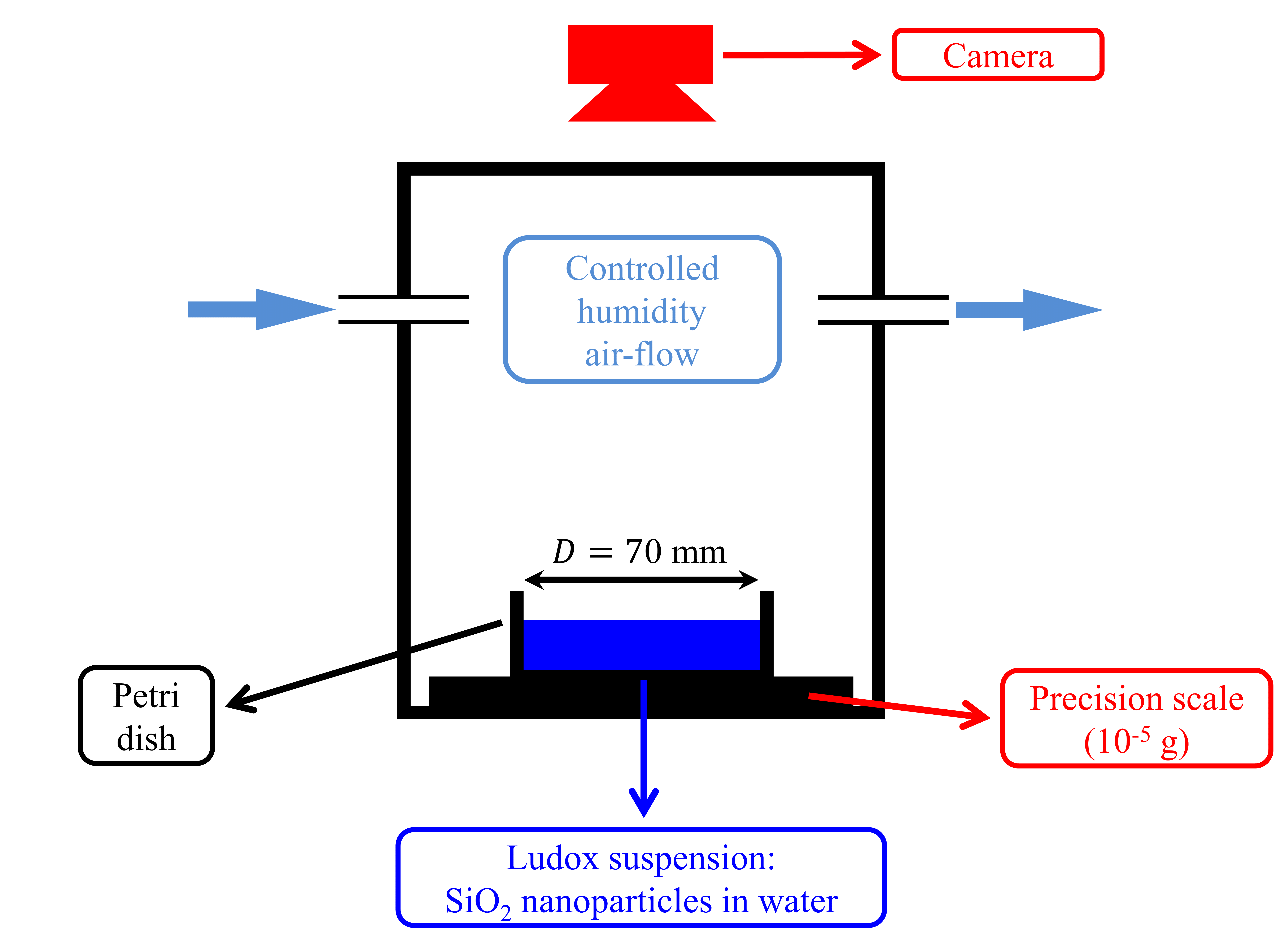
During the drying experiment, decreases as water evaporates off the suspension. After some time, the mass of the drying layer stabilizes to its final value. Nevertheless, samples dried at high may retain a significant amount of water in their pores (up to in mass). This may be due to capillary condensation at the nanopores in the solid layer. As water evaporates from the suspension, the free surface of the liquid gradually moves down; the corresponding speed, called the evaporation rate or drying rate, can be expressed as :
| (8) |
where is the mass loss rate and is the density of water. During the first phase of colloidal drying, the mass loss is nearly linear with time; that is, and are constants, respectively coined and . In the rest of article, the expression "drying rate" will refer to the initial drying rate .
In the dilute phase, the evaporation rate for the silica suspension is that of pure water. As such, it is expected to be proportional to .(Coussot 2000) This relation has been verified for the four suspensions, over the whole range of explored (Fig. 3). Hereafter, (rather than ) is set as the control parameter.

II.3 Bulk packing fraction measurement
The packing fraction of the dry colloidal layers can be defined as the proportion of solid volume, , to the total volume, : . The tightness of the particle packing can also be described using the porosity, . This is defined as , where is the pore volume (with ). Calculating requires to measure at least two parameters among the three ones: , and . In this study, was inferred from and .
The volume occupied by the solid particles can be expressed as , where is the mass of the dry sample and the density of the silica. The mass was measured after three hours of heat treatment at , in order to evaporate off all water retained in the pores of the dried silica layer. In order to estimate the density of the silica particles, a dilution method, outlined in,(Caddock and Hull 2002) was invoked on the HS-m suspension. Several dilutions of HS-m were prepared at prescribed mass fractions and their densities were measured. From the relationship , where is the density of water, a linear regression yielded .
An accurate method for the determination of total volume invokes hydrostatic weighting.Lesaine et al. 2018 First, a sample of dried suspension was soaked in water. At immersion, air bubbles are observed and a penetration front visibility progresses though the morsel. Samples were soaked for several hours prior to measurement, until these two processes ceased completly (meaning the morsel was visually homogeneous with stable mass). After soaking, the samples were weighed in air (mass ) and in water (apparent mass ) using a standard hydrostatic weighing protocol. Prior to weighing, the water present on the sample surface was removed through careful wiping. As the water-soaked sample is left to dry in air, its measured mass decreases. This mass loss is quickly accompanied by a change in the visual appearance of the morsel, which become opaque. After soaking and blotting, by measuring the sample mass immediately, before opacification, we ensured the amount of water loss by evaporation was negligible. Tests showed the whole procedure to be well reproducible: Repeating the soaking and weighing procedure on few samples (mass ), the same mass was measured within , corresponding to less than mass variation.
Once and are measured, is deduced from Archimedes’ principle: . Note that if the pores are only partially filled, this will equally affect and and cancel out in the expression of . Thus, the accuracy of this method does not require the complete filling of the pores by the fluid, in contrast to other methods such as gas pycnometry or mercury porosimetry.
For each drying experiment, packing fraction measurements were repeated on two morsels. For HS-m layers, one morsel was soaked and weighted in water, and another one in ethanol. The density of the ethanol bath increased slightly with time; this is probably due to water absorption from the atmosphere. Porosity measurements on the layers obtained from the three other suspensions (HS-p, SM and TM) were made using water for all the morsels.
II.4 AFM imaging of the nanoscale particle arrangement at the layer surface
In order to obtain spatial information on particle position, we used atomic force microscopy (AFM) to image the dried surfaces. A Bruker Dimension Icon Nanoscope V mounted with radius tips (MPP-11220-10, and then RTESPA-300 tips) provided images of the surfaces of the dried morsels in Tapping mode. For each drying experiment, a morsel was taken after drying and placed under the AFM head. To enable the averaging of surface properties, multiple images (, ) were taken on the drying surface of each sample. As the samples are quite abrasive, tip wear occurs rapidly. The tip was thus replaced as soon as wear would degrade image quality, usually after 5 to 10 images.

In order to compute statistics on the arrangement of the colloidal particles, it is necessary to extract the position of the particle centers from the topographical AFM images. To do so, a Matlab routine has been developed to allow the detection of all the local height maxima in a given image. Figure 4 represents a typical output of this routine.
III Experimental results: Effect of drying rate and particle size distribution on dry layer nanostructure
III.1 Surface nanostructure: crystalline vs amorphous


Figure 5, left column presents typical AFM images of the dry silica layers surfaces. The corresponding 2-D Fourier spectra, shown on the right column, provide a direct visualization of the crystalline or amorphous nature of the arrangements. Depending on suspension type and drying rate, either a hexagonal structure or amorphous packings are observed. In short:
- •
- •
- •
Layers prepared from TM suspension (Fig. 5, row 5) exhibit clear crystallinity at all drying rates. Note that both first-order and second-order diffraction peaks are visible on the 2D Fourier spectra.
III.2 Surface nanostructure: translational & rotational order
Extracting the positions of the particle centers from the AFM images allows for a quantitative characterization of surface structure in the dry layers.
Long-range translational order can be characterized using the pair correlation function . This function represents the probability of finding a particle center at a distance from a given particle, normalized by the probability for an ideal gas ( for random non-correlated particle positions).Hansen and McDonald 2013 Figure 6 shows for all four suspensions at maximal (blue, top curves) and minimal (red, bottom curves) drying rates. TM layers and fast-dried () HS-m layers exhibit well-defined long-range peaks, which are the signature of long-range translational order. Conversely, functions for slowly-dried () HS-m layers, as well as for SM and HS-p layers, lack such peaks for larger than two particle diameters. Thus, no translational order exists at the surface of these layers.

Crystallinity at the drying surface can be further characterized using the bond angle order parameter , defined by:Reis et al. 2006
| (9) |
where is the number of nearest neighbors, is the number of particles in the AFM image, the number of nearest neighbors for particle , and is the angle between a fixed direction and the line joining particles and . For a hexagonal arrangement, as observed on our layers, . is a measure of the orientational order of the particle arrangement. For an amorphous arrangement, , while for an arrangement with sixfold symmetry (such as a perfect hexagonal lattice), . Figure 7 gives as a function of the drying rate for each of the four Ludox suspensions.

For all SM and HS-p layers, (Figs. 7A and 7B), which suggests that the layers are amorphous, irrespectively of the drying rate. This is in agreement with the profiles on these layers, which show no crystalline peaks (Figs. 6A and 6B) beyond the next nearest neighbor. Conversely, for TM layers (Fig. 7C), a value indicative of crystallinity. This is also consistent with the peaks observed in for these layers (Fig. 6C). HS-m layers show two regimes, one with an amorphous structure () at low evaporation rates (), and one with increasing crystallinity for , with at the highest evaporation rate (Fig. 7D). Even in the most crystalline layers, the particle centers are not perfectly aligned with the vertices of a hexagonal lattice. Moreover, thermal drift can introduce distortion in the AFM image, as can be seen for example on Fig. 5, row 5. Hence, is always significantly lower than one.
III.3 Bulk packing fraction
The previous section concerned the characterization of particle arrangement at the surface of the dried layer. We now turn to the analysis of bulk structure via the measurement of packing fraction. Figure 8 presents the packing fraction as a function of drying rate for the layers obtained from the four suspensions. Error bars are larger on the lower side, as they take into account the possible presence of water at the surface of the nanoparticles, which could overestimate by up to .(Iler 1979)

In all cases, the packing fraction increases with increasing drying rate; hence, slowly dried layers are more porous. In HS-m and HS-p suspensions, a plateau is clearly observed for . Volume fraction saturates at a value , very close to the random close packing value ( for monodisperse packing) and far below the value expected for 2D crystalline structures ( for monodisperse packing). In other words, even in HS-m layers which exhibits crystalline particle arrangement at the surface, the bulk is to a large extend amorphous, even at the highest drying rate. The range of volume fraction observed in SM layers is much smaller, around . Conversely, is much higher in TM layers, up to , which suggests that crystallization may extend significantly within the layer bulk. Figure 9 gathers on a single graph the curves of as a function of for the four suspensions. It demonstrates the absence of univocal relationship between bulk volume fraction and surface arrangement: Crystalline surface arrangements are only observed in dense layers (), while amorphous surface arrangements () can be associated with either loose or dense packing, depending on evaporation rate and particle size and dispersity.
In summary, this series of results show that:
- •
Low dispersity is required to observe surface crystallization: Crystallization is observed in all TM layers () and on some HS-m layers (), but never on SM layers () nor on HS-p layers ().
- •
Crystallization is favored by increased evaporation rate, as observed on HS-m.
It is worth noting that this second observation may appear counter-intuitive; the slow evolution of a system generally favors order formation. A possible explanation to this counter-intuitive result was advanced in,Piroird et al. 2016 by postulating that slow evaporation favored the formation of aggregates, thus precluding particle crystallization. The following section takes a closer look at this hypothesis by putting it to test.
IV Evidence of particle aggregation at low evaporation rates
Checking the postulate in Piroird et al.,Piroird et al. 2016 we invoked SAXS measurements in conjunction with holding period experiments for the HS-m suspension, which was found to exhibit a disorder-to-order transition driven by the drying rate. During a holding period experiment, the suspension is first dried at the highest evaporation rate, in order to make the suspension more concentrated. The drying is then interrupted for a prescribed time, while the suspension is still in a liquid state (Fig. 10A). Finally, the drying resumes at the original rate until completion. A fast-drying experiment yields a crystalline layer (Fig. 10B), yet a holding period experiment yields an amorphous one (Fig. 10C). Postulating the aggregate formation, this could be explained as follow: When the suspension remains long enough in a concentrated liquid state, whether during a slow-drying experiment or during a holding period, aggregates form. Once formed, they preclude the crystallization of the particles in the dried layer, regardless of the drying rate.

SAXS measurements can now provide information on the actual formation of aggregates in the suspension during the holding period. The scattering curve of the particles in suspension was measured at the beginning and the end of the holding period. of HS-m suspension were dried at the highest evaporation rate (, ) down to a mass . of this concentrated suspension were sampled, diluted, and measured in SAXS, invoking the same dilution and measurement protocols as for the suspensions characterization (see Sec 2.1). The rest of the suspension was subjected to a holding period (); this aged suspension was then in turn diluted and measured in SAXS.
Figure 10D represents the scattering curve of the sampled suspension, at the beginning of the holding period (solid blue line) and after the seven-day holding period (red dashed line). Before aging, approaches a constant value at low , which is indicative of a suspension of monodisperse particles. After the seven day holding period, follows a power law at low (corresponding to a constant slope in log-log plot). A linear regression confirms that for q < 0.3 nm-1, with an exponent . This is indicative of the formation of loose aggregates with a fractal dimension .Moro et al. 2017 The evolution of the scattered intensity at low thus demonstrates the formation of aggregates in the concentrated suspension. This substantiates the scenario initially proposed in.Piroird et al. 2016
V Discussion
This experimental study was designed to shed light on how colloidal particles self-assemble upon drying and form a solid layer of a given nanostructure. In this context, we examine bulk volume fraction and particle arrangement at the surface of solid layers obtained by drying millimeter-thick suspensions of silica nanospheres, using particle size and evaporation rate as control parameters. The principal results from our observations are:
- (i)
Either crystalline or amorphous particle arrangements can be observed at the surface of the dried layer: Amorphous structures are always observed in SM, crystalline structures are always observed in TM, and either crystalline or amorphous structures are observed in HS depending on drying rate and polydispersity. This observation can be compared with the reflectivity and scattering measurements inLéang et al. 2019 showing that the degree of ordering increases with increasing particle size for the same types of Ludox suspensions.
- (ii)
Crystallization requires both sufficiently high drying rate and low polydispersity. The two most polydisperse dispersions (SM and HS-p) never crytallize. This is consistent with molecular dynamics simulations of hard spheres systems.Pusey et al. 2009. The threshold dispersity value for Ludox surface crystallization is observed to lie between 14 and 19 .
- (iii)
Crystalline surface arrangements imply dense bulk packing. Conversely, amorphous surfaces are observed in dry layers with either loose or dense bulk packing.
- (iv)
When surface crystallization happen, the bulk volume fraction can reach values of up to , which is significantly larger than the random close packing value ( for monodisperse packings). Though polydispersity is known to increase , Phan et al. 1998; Farr and Groot 2009 this increase is expected to be very small: for a log-normal size distribution of dispersity .Farr and Groot 2009 Hence, this alone cannot explain the value observed in TM. This suggests that the crystallization is not limited to the surface, but extend through the bulk, even in these millimeter-thick layers. Note that, in the case of crystalline close packing, polydispersity make volume fraction smaller.Phan et al. 1998 This may explain why the observed value is smaller than the value expected for crystalline closed packing of monodisperse spheres.
Table 3 summarizes the interrelations between drying rate and particle size distribution on one hand, and surface order and bulk density on the other hand.
| Suspension | SM | HS-m | HS-p | TM |
| Size, | ||||
| pH | 9.2-9.9 | |||
| Dispersity | 0.14 | |||
| Surface (low ) | amorphous | amorphous | amorphous | ordered |
| Surface (high ) | amorphous | ordered | amorphous | ordered |
| Bulk (low ) | low | medium | medium | high |
| Bulk (high ) | low | high | high | high |
Peclet number, , is usually considered as the relevant dimensionless parameter to rationalize how evaporation rate selects final packing structure. Routh and Zimmerman 2004; Ekanayake et al. 2009 writes where is the suspension thickness at drying initiation, and is the diffusion coefficient for the colloids. This number represents the ratio between Brownian diffusion time and particle convection time toward the surface, which corresponds also to the layer evaporation timescale . High indicates directional drying with a solid formed at the surface layer by layer, while low means isotropic bulk compression as water evaporates. To check whether or not controls final packing structure, we considered the experiments in HS-m.Piroird et al. 2016 Using Stokes-Einstein relation, one gets in HS-m at . From Fig. 7D, experiments achieved with (i.e. ) should promote crystalline surface arrangement. This has been tested by performing an additional experiment Piroird et al. 2016 in HS-m at a lower drying rate (), but starting with a suspension thickness twice larger (). Peclet number in this additional experiment is , i.e. much larger than . Still, the particle arrangement was observed to be amorphous and not crystalline. This demonstrates that is not the relevant parameter driving particle packing in the experiments reported here. Beyond convection and diffusion captured by Peclet number, a third ingredient necessarly plays a key role in the selection of the final dried layer nanostructure.
The holding period experiment and SAXS measurements reported in Sec. 4 demonstrate that slow drying allows the formation of particle aggregates in the liquid phase. We argue this flocculation process to be this missing ingredient. Crystallization will be observed provided:
- (i)
low enough polydispersity;
- (ii)
flocculation is precluded before solidification.
Requirement (i) is fulfilled in TM and HS-m suspensions since crystallization is observed for some drying conditions. Requirement (ii) is fulfilled in these two suspensions for fast enough drying, when evaporation timescale, , is smaller than aggregation timescale, . In HS-m, this is ensured for , i.e. for . This value provides an order of magnitude for aggregation timescale in HS-m: . This is consistent with the observation that introducing an holding period of in a fast drying experiment promotes the aggregate formation, and subsequently precludes packing order at the dried layer surface. In TM, crystallinization is observed over the whole range of explored , down to . This means that aggregation time in TM is larger than : . The fact that can be understood since colloids in TM are larger. Hence, the diffusion coefficient is smaller, diffusion time is larger, and finally, as increases with ,Lin et al. 1989 aggregation time is larger. In SM, no crystallinisation is observed over the whole range of explored , up to . This means that either requirement (i) or (ii) are not fulfilled (or both): Either the polydispersity is too high to allow crystallization, or the aggregation time is too small, , to allow preclude flocculation in our drying experiments. Finally, in HS-p, no crystallinization is observed. The main difference between HS-p and HS-m is that polydispersity is much larger in HS-p (, compared to for HS-m); hence the absence of crystallinisation in HS-p is due to the failure of requirement (i).
Variations in volume fraction provide another signature of flocculation. Large aggregates cannot pack very densely and must yield more porous layers. Consequently, large volume fractions are expected in TM since flocculation is precluded over the whole range of explored . Conversely, the small volume fractions observed in SM at all suggest that aggregation is important over the whole range of explored drying rate; this suggests that the failure of requirement (ii) rather than failure of requirement (i) is responsible for the absence of crystallinization in SM. For intermediate cases (HS-m and HS-p), layer density depends on the aggregate formation and is mediated by the drying rate. Note that in Ludox HS, dispersity does not have a significant effect on packing fraction: the porosities observed in HS-m and HS-p are roughly the same. It may be important at larger particle sizes, for which flocculation seems to be prevented. In the TM suspension, indeed, volume fraction is significantly larger than the RCP value ( to be compared with in monodisperse packings); this suggests that surface ordering extends partially through the layer bulk. The way order and disorder coexist in the 3D bulk remains an open question. In this context, it is worth noting that a similar phenomenon of packing ordering promoted by faster colloid velocity has been reported by Noirjean et al.Noirjean et al. 2017 during unidimensional drying in a 2D Hele-Shaw cell opened on one side. Direct imaging of the colloid arrangement during drying was possible in such a 2D geometry, and it was evidenced a succession of ordered and disordered domains with thickness of particle size. Similar organization may occurs in our 3D drying geometry. TEM imaging of the layer cross-section could provide further information on this aspect.Yotsumoto and Yoon 1993
VI Conclusion
The series of experiments reported here investigated how particles self-assemble during colloidal drying to form thick solid layers with varying nanostructures. In dispersions with hard, non deformable particles, such as the silica suspensions examined here, particle arrangement in the dried layer is demonstrated to be mediated by flocculation. This process occurs in the liquid phase. Aggregate formation depends on the drying rate, as reported in:Piroird et al. 2016 slower evaporation leaves more time for flocculation to proceed and thus allows larger aggregates to form. In the systems and for the drying conditions examined here, final packing structure is mainly driven by the ratio of aggregation time over evaporation/convection time, rather than by the Peclet number (Brownian diffusion time over convection time) as is sometimes the case. Routh and Zimmerman 2004; Ekanayake et al. 2009 This highlights that in general, both ratios shall be considered when the packing structure is investigated. Selection of aggregation time in presence of evaporation remains an open question: It is expected to increase with diffusion timeLin et al. 1989 and, as such, to increase with colloid size. It should also depend on the dispersion stability at the onset of evaporation. Future measurements of the zeta potential during drying may shed a new light on this aspect. Indeed, starting with Smoluchowski coagulation equation Smoluchowski 1917 and Derjaguin-Landau-Verwey-Overbeek (DLVO) theory, Derjaguin and Landau 1941; Verwey and Overbeek 1947 a series of increasingly sophisticated models Spielman 1970; McGown and Parfitt 1967; Honig et al. 1971; Bremer et al. 1995; Grasso et al. 2002; Lachin et al. 2019 has been developped to assess colloidal stability and flocculation kinetics (see e.g. Russel et al. 2012 for recent reviews). They may allow an estimation of the aggregation time from the knowledge of the ion concentration, zeta potential and Hamaker constant.
Depending on the extent of flocculation, dried layers of variable density are obtained : the smaller the aggregates, the higher the bulk volume fraction. When flocculation is precluded and the initial particle dispersity is low enough (less than ), crystallization is observed at the layer surface. As demonstrated here in Ludox TM, crystalline arrangement of the particle can also extend in 3D through the layer bulk, even in millimeter-thick dry layers.
These results may be of interest in the design of processes requiring the auto-assembly of colloidal particles into large-scale crystalline structures, for example for photonics and biotechnology applications. They also shed a new light on why increasing drying rate yields more cracks in the dried layer:Gauthier et al. 2010; Boulogne et al. 2014 because of flocculation, slower drying yields more porous layers. Moreover, the elastic moduli of these layers is a decreasing function of volume fraction.Lesaine et al. 2018 Then, slower drying yields softer layers, which can accommodate capillary and/or substrate induced tension more easily, without cracking. This scenario is of course to be confirmed, as the crack patterns depends on the balance between available elastic energy and fracture costsGauthier et al. 2010; Maurini et al. 2013; Lazarus 2017 in which many other mechanisms can be involved (chemical bond tightening increasing with time or dependence of the stress evolution with drying rateChekchaki and Lazarus 2013 for instance). Work in this direction is under progress.
Conflicts of interest
There are no conflicts to declare.
Acknowledgements
The co-authors of this work would like to acknowledge financial support from Triangle de la Physique (RTRA), Ile-de-France (C’Nano, ISC- PIF, and DIM-Map), LabEx LaSIPS (ANR-10-LABX- 0040-LaSIPS) and PALM (ANR-10-LABX-0039-PALM) managed by the French National Research Agency under the "Investissements d’avenir" program (ANR-11-IDEX-0003-02).
References
- Attinger et al. (2013) D. Attinger, C. Moore, A. Donaldson, A. Jafari and H. A. Stone, Forensic Science International, 2013, 231, 375–396.
- Tang et al. (2011) C.-S. Tang, Y.-J. Cui, B. Shi, A.-M. Tang and C. Liu, Geoderma, 2011, 166, 111–118.
- Routh (2013) A. F. Routh, Reports on Progress in Physics, 2013, 76, 046603.
- Joseph Keddie (2010) A. F. R. Joseph Keddie, Fundamentals of Latex Film Formation, Springer-Verlag GmbH, 2010.
- Brinker and Scherer (1990) C. Brinker and G. Scherer, Sol-Gel Science, Academic Press, 1990.
- Colvin (2001) V. L. Colvin, MRS Bulletin, 2001, 26, 637–641.
- Vlasov et al. (2001) Y. A. Vlasov, X.-Z. Bo, J. C. Sturm and D. J. Norris, Nature, 2001, 414, 289–293.
- Blanco et al. (2000) A. Blanco, E. Chomski, S. Grabtchak, M. Ibisate, S. John, S. W. Leonard, C. Lopez, F. Meseguer, H. Miguez, J. P. Mondia, G. A. Ozin, O. Toader and H. M. van Driel, Nature, 2000, 405, 437–440.
- Goehring et al. (2015) L. Goehring, A. Nakahara, T. Dutta, S. Kitsunezaki and S. Tarafdar, Desiccation cracks and their patterns: Formation and modelling in Science and Nature, Wiley, 2015.
- Lesaine et al. (2018) A. Lesaine, D. Bonamy, G. Gauthier, C. L. Rountree and V. Lazarus, Soft Matter, 2018, 14, 3987.
- Lesaine (2018) A. Lesaine, Ph.D. thesis, Université Paris-Saclay, 2018.
- Gauthier et al. (2010) G. Gauthier, V. Lazarus and L. Pauchard, EPL (Europhysics Letters), 2010, 89, 26002.
- Lazarus and Pauchard (2011) V. Lazarus and L. Pauchard, Soft Matter, 2011, 7, 2552–2559.
- Giorgiutti-Dauphiné and Pauchard (2014) F. Giorgiutti-Dauphiné and L. Pauchard, The European Physical Journal E, 2014, 37, 1–7.
- Lazarus (2017) V. Lazarus, Europhysics Letters, 2017, 117, 24002.
- Caddock and Hull (2002) B. D. Caddock and D. Hull, Journal of Materials Science, 2002, 37, 825–834.
- Boulogne et al. (2014) F. Boulogne, F. Giorgiutti-Dauphiné and L. Pauchard, Oil Gas Sci. Technol. – Rev. IFP Energies nouvelles, 2014, 69, 397–404.
- Narayanan et al. (2004) S. Narayanan, J. Wang and X.-M. Lin, Physical Review Letters, 2004, 93, 135503.
- Bigioni et al. (2006) T. P. Bigioni, X.-M. Lin, T. T. Nguyen, E. I. Corwin, T. A. Witten and H. M. Jaeger, Nature Materials, 2006, 5, 265–270.
- Marín et al. (2011) Á. G. Marín, H. Gelderblom, D. Lohse and J. H. Snoeijer, Physical Review Letters, 2011, 107, 085502.
- Monteux and Lequeux (2011) C. Monteux and F. Lequeux, Langmuir, 2011, 27, 2917–2922.
- Askounis et al. (2013) A. Askounis, K. Sefiane, V. Koutsos and M. E. R. Shanahan, Physical Review E, 2013, 87, 012301.
- Goehring et al. (2010) L. Goehring, W. J. Clegg and A. F. Routh, Langmuir, 2010, 26, 9269–9275.
- Inasawa et al. (2016) S. Inasawa, Y. Oshimi and H. Kamiya, Soft Matter, 2016, 12, 6851–6857.
- Noirjean et al. (2017) C. Noirjean, M. Marcellini, S. Deville, T. E. Kodger and C. Monteux, Phys. Rev. Materials, 2017, 1, 065601.
- You et al. (2017) J. You, J. Wang, L. Wang, Z. Wang, Z. Wang, J. Li and X. Lin, Colloids and Surfaces A: Physicochemical and Engineering Aspects, 2017, 531, 93–98.
- Piroird et al. (2016) K. Piroird, V. Lazarus, G. Gauthier, A. Lesaine, D. Bonamy and C. L. Rountree, EPL, 2016, 113, 38002.
- Orts-Gil et al. (2010) G. Orts-Gil, K. Natte, D. Drescher, H. Bresch, A. Mantion, J. Kneipp and W. Österle, Journal of Nanoparticle Research, 2010, 13, 1593–1604.
- Teulon et al. (2018) J.-M. Teulon, C. Godon, L. Chantalat, C. Moriscot, J. Cambedouzou, M. Odorico, J. Ravaux, R. Podor, A. Gerdil, A. Habert, N. Herlin-Boime, S. wen Chen and J.-L. Pellequer, Nanomaterials, 2018, 9, 18.
- Feigin and Svergun (1987) L. A. Feigin and D. I. Svergun, Structure Analysis by Small-Angle X-Ray and Neutron Scattering, Plenum Press, 1987.
- Pedersen (1997) J. S. Pedersen, Advances in Colloid and Interface Science, 1997, 70, 171–210.
- Li et al. (2016) J.-G. Li, G. Fornasieri, A. Bleuzen, M. Gich, A. Gloter, F. Bouquet and M. Impéror-Clerc, Small, 2016, 12, 5981–5988.
- Zeng et al. (2011) Y. Zeng, S. Grandner, C. L. P. Oliveira, A. F. Thünemann, O. Paris, J. S. Pedersen, S. H. L. Klapp and R. von Klitzing, Soft Matter, 2011, 7, 10899.
- Gauthier et al. (2007) G. Gauthier, V. Lazarus and L. Pauchard, Langmuir, 2007, 23, 4715–4718.
- Giuseppe et al. (2012) E. Giuseppe, A. Davaille, E. Mittelstaedt and M. François, Rheologica Acta, 2012, 51, 451–465.
- Coussot (2000) P. Coussot, The European Physical Journal B, 2000, 15, 557–566.
- Hansen and McDonald (2013) J.-P. Hansen and I. R. McDonald, Theory of Simple Liquids; with Applications to Soft Matter, Elsevier LTD, 2013.
- Reis et al. (2006) P. M. Reis, R. A. Ingale and M. D. Shattuck, Physical Review Letters, 2006, 96, 258001.
- Iler (1979) R. Iler, The Chemistry of Silica, Wiley, 1979.
- Moro et al. (2017) S. Moro, C. Parneix, B. Cabane, N. Sanson and J.-B. d’Espinose de Lacaillerie, Langmuir, 2017, 33, 4709–4719.
- Léang et al. (2019) M. Léang, D. Lairez, F. Cousin, F. Giorgiutti-Dauphiné, L. Pauchard and L.-T. Lee, Langmuir, 2019, 35, 2692–2701.
- Pusey et al. (2009) P. N. Pusey, E. Zaccarelli, C. Valeriani, E. Sanz, W. C. K. Poon and M. E. Cates, Philosophical Transactions of the Royal Society A: Mathematical, Physical and Engineering Sciences, 2009, 367, 4993–5011.
- Phan et al. (1998) S.-E. Phan, W. B. Russel, J. Zhu and P. M. Chaikin, The Journal of Chemical Physics, 1998, 108, 9789–9795.
- Farr and Groot (2009) R. S. Farr and R. D. Groot, The Journal of Chemical Physics, 2009, 131, 244104.
- Routh and Zimmerman (2004) A. F. Routh and W. B. Zimmerman, Chemical Engineering Science, 2004, 59, 2961–2968.
- Ekanayake et al. (2009) P. Ekanayake, P. J. McDonald and J. L. Keddie, The European Physical Journal Special Topics, 2009, 166, 21–27.
- Lin et al. (1989) M. Y. Lin, H. M. Lindsay, D. A. Weitz, R. C. Ball, R. Klein and P. Meakin, Nature, 1989, 339, 360–362.
- Yotsumoto and Yoon (1993) H. Yotsumoto and R.-H. Yoon, Journal of Colloid and Interface Science, 1993, 157, 434–441.
- Smoluchowski (1917) M. Smoluchowski, Z. Phys. Chem., 1917, 92, 68.
- Derjaguin and Landau (1941) B. Derjaguin and L. D. Landau, Acta Physicochimica U.R.S.S., 1941, 14, 633–662.
- Verwey and Overbeek (1947) E. J. W. Verwey and J. T. G. Overbeek, The Journal of Physical and Colloid Chemistry, 1947, 51, 631–636.
- Spielman (1970) L. A. Spielman, Journal of Colloid and Interface Science, 1970, 33, 562–571.
- McGown and Parfitt (1967) D. N. L. McGown and G. D. Parfitt, The Journal of Physical Chemistry, 1967, 71, 449–450.
- Honig et al. (1971) E. P. Honig, G. J. Roebersen and P. H. Wiersema, 1971, 36, 97–109.
- Bremer et al. (1995) L. G. Bremer, P. Walstra and T. van Vliet, Colloids and Surfaces A: Physicochemical and Engineering Aspects, 1995, 99, 121–127.
- Grasso et al. (2002) D. Grasso, K. Subramaniam, M. Butkus, K. Strevett and J. Bergendahl, Reviews in Environmental Science and Bio/Technology, 2002, 1, 17–38.
- Lachin et al. (2019) K. Lachin, N. L. Sauze, N. D. M. Raimondi, J. Aubin, M. Cabassud and C. Gourdon, Chemical Engineering Journal, 2019, 369, 818–827.
- Russel et al. (2012) W. B. Russel, D. A. Saville and W. R. Schowalter, Colloidal Dispersions, Cambridge University Press, 2012.
- Maurini et al. (2013) C. Maurini, B. Bourdin, G. Gauthier and V. Lazarus, International Journal of Fracture, 2013, 184, 75–91.
- Chekchaki and Lazarus (2013) M. Chekchaki and V. Lazarus, Transport in Porous Media, 2013, 100, 143–157.