跳到论文正文
W Papers独立论文阅读器 arXiv:2012.05461 论文正文 计算阅读时间 · 0%
引用这篇论文根据当前论文元数据生成,正式投稿前建议核对。


License: arXiv.org perpetual non-exclusive license
arXiv:2012.05461v1 [cond-mat.supr-con] 10 Dec 2020

Weak Localization Correction to Linear Absorption in Conventional Superconductors

Takanobu Jujo Thanks: E-mail address: jujo@ms.aist-nara.ac.jp
Abstract

The weak localization effect on a linear absorption spectrum is investigated for disordered s-wave superconductors. The vertex correction is incorporated into the response function in a way that is consistent with the weak localization correction to a one-particle spectrum. The effect of interactions between electrons enhanced by their diffusive motion makes a major contribution to the correction term. Numerical calculations show that the weak localization effect suppresses the absorption by the excitation across the gap to a greater extent than that by thermal excitation, which is a similar tendency to the results of experiments. The ratio of the linear absorption with vertex corrections to that without the corrections shows a large variation at the frequency that is around twice the energy of the superconducting gap. This behavior represents a relationship between the weak localization effect on the linear absorption and that on the one-particle spectrum.

1 Introduction

The weak localization effect has so far been studied mainly in the normal state. In the case of the noninteracting electron systems, a correction term in conductivity arises from the coherent backscattering by impurities. [1] The motion of electrons becomes diffusive in the presence of the impurity scattering, and electron–electron interactions such as the screened Coulomb interaction are modified. [2, 3, 4] This effect also gives a weak localization correction to the dc and ac conductivities. [4, 5, 6]

Through the same effect, the superconducting transition temperature TcT_{c} is lowered because the interactions between electrons change owing to the impurity scattering. [7, 8, 9] In the case of the superconducting state, there have been few studies on weak localization effect other than the correction to TcT_{c}. For example, superfluid density is calculated considering only the effect of backscattering by impurities. [10] As for the conductivity, the influence of superconducting fluctuation becomes strong near the transition temperature. [11, 12, 13] This fluctuation effect on ac conductivity has been investigated in the normal state, [14, 15, 16, 17] but the effect of the Coulomb interaction has not been taken into account in these studies.

In the presence of the superconducting gap (Δ\Delta) (when the temperature is below the transition temperature), the real part of ac conductivity takes finite values at a frequency (ω\omega) lower than twice the superconducting gap owing to thermally excited quasiparticles. In the case of ω>2​Δ\omega>2\Delta, there exists a finite absorption even at absolute zero owing to the excitation across the gap. [18, 19] This behavior of ac conductivity is described by the Mattis–Bardeen (MB) formula.

In recent years, deviations from the MB formula have been observed experimentally in strongly disordered systems. [20, 21, 22] These studies show that the absorption for ω<2​Δ\omega<2\Delta is large and the spectrum at the gap edge (ω≃2​Δ\omega\simeq 2\Delta) becomes blurred as compared with that obtained on the basis of the MB theory. This phenomenon has been interpreted with several ideas, such as the pair-breaking effect by nonuniformity, [23] collective excitation modes, [24] or the existence of a normal (Drude) component. [21] These systems are considered to be situated near the superconductor–insulator transition and have inhomogeneities. It is yet unknown whether these systems reflect the weak localization effect partly because there is no theory about this correction effect in the superconducting state.

In this study, we show how the weak localization effect appears in the ac conductivity of superconductors in a homogeneously disordered system. The conductivity including vertex corrections is calculated in a three-dimensional system, in which the expansion parameter is 1/(kF​l)21/(k_{F}l)^{2} where kFk_{F} is the Fermi wave number and l=vF​τl=v_{F}\tau is the mean free path (vFv_{F} and τ\tau being the Fermi velocity and the relaxation time, respectively). We derive vertex corrections from the functional derivative of self-energy. The latter gives a weak localization correction to a one-particle spectrum in the superconducting state. [25] According to the calculated results, it is found that the weak localization correction is larger for ω>2​Δ\omega>2\Delta is larger than for ω<2​Δ\omega<2\Delta. Taking the ratio of the correction term to the MB conductivity clarifies how the correction effect on the linear absorption is related to that on the one-particle spectrum.

The structure of this paper is as follows. Section 2 gives a formulation for calculating response functions including the impurity scattering and interactions between electrons. In Sect. 3, a formula for the conductivity including vertex corrections that give a weak localization effect is obtained. Section 4 gives the results of numerical calculations on the basis of obtained expressions for the conductivity.

2 Formulation

We calculate the ac conductivity σq\sigma_{q} by Keldysh’s method [26] with the use of the functional integral. [27] The absorption spectrum is given by the real part of the ac conductivity, and it is written as

Re​σq=−Im​Kqω.{\rm Re}\sigma_{q}=-\frac{{\rm Im}K_{q}}{\omega}. (1)

“Re{\rm Re}” and “Im{\rm Im}” indicate the real and imaginary parts, respectively. q=(\mib​q,ω)q=(\mib q,\omega) with \mib​q\mib q being the wave number vector in three dimensions. We consider only the uniform case (\mib​q=\mib​0)(\mib q=\mib 0) and finite frequencies (ω≠0\omega\neq 0), and set ℏ=c=1\hbar=c=1 in this paper. KqK_{q} is a response function and defined with the current density JqJ_{q} as

Jq=−Kq​Aq,J_{q}=-K_{q}A_{q}, (2)

where AqA_{q} is the vector potential. We consider an isotropic system and omit indices of vectors. The current density is derived from the functional derivative of the action (SS) by the vector potential:

Jq=−i2​δ​ln​⟨ei​S⟩e,p,iδ​A−qq​u|Aq​u→0.J_{q}=\left.\frac{-i}{\sqrt{2}}\frac{\delta{\rm ln}\langle{\rm e}^{iS}\rangle_{e,p,i}}{\delta A_{-q}^{qu}}\right|_{A^{qu}\to 0}. (3)

Here, Aqq​uA^{qu}_{q} is the Fourier transform of A\mib​q,tq​u:=(A\mib​q,t+−A\mib​q,t−)/2A^{qu}_{\mib q,t}:=(A^{+}_{\mib q,t}-A^{-}_{\mib q,t})/\sqrt{2} with A\mib​q,t+(−)A^{+(-)}_{\mib q,t} being the vector potential in the forward (backward) direction in time. [27] The vector potential in Eq. (2) is given by the Fourier transform of (A\mib​q,t++A\mib​q,t−)/2(A^{+}_{\mib q,t}+A^{-}_{\mib q,t})/2 (=:A\mib​q,tc​l/2)(=:A^{cl}_{\mib q,t}/\sqrt{2}). We consider the following action:

S=∫𝒞dt{∑\mib​k,σψ¯\mib​k,σ,t(i∂t−ξ\mib​k)ψ\mib​k,σ,t−(2N3)−1∑\mib​k,\mib​k′,\mib​q,σ,σ′v\mib​qCψ¯\mib​k,σ,tψ\mib​k+\mib​q,σ,tψ¯\mib​k′,σ′,tψ\mib​k′−\mib​q,σ′,t+∑\mib​qb¯\mib​q,t(i∂t−ω\mib​q)b\mib​q,t+(N3)−1/2∑\mib​k,\mib​q,σψ¯\mib​k+\mib​q,σ,t[e\mibA\mib​q,t⋅\mibv\mib​k+\mib​q/2−gp​hϕ\mib​q,t−u\mib​q]ψ\mib​k,σ,t}.\begin{split}S=&\int_{\cal C}dt\{\sum_{\mib k,\sigma}\bar{\psi}_{\mib k,\sigma,t}(i\partial_{t}-\xi_{\mib k})\psi_{\mib k,\sigma,t}-(2N^{3})^{-1}\sum_{\mib k,\mib k^{\prime},\mib q,\sigma,\sigma^{\prime}}v_{\mib q}^{C}\bar{\psi}_{\mib k,\sigma,t}\psi_{\mib k+\mib q,\sigma,t}\bar{\psi}_{\mib k^{\prime},\sigma^{\prime},t}\psi_{\mib k^{\prime}-\mib q,\sigma^{\prime},t}\\ &+\sum_{\mib q}\bar{b}_{\mib q,t}(i\partial_{t}-\omega_{\mib q})b_{\mib q,t}+(N^{3})^{-1/2}\sum_{\mib k,\mib q,\sigma}\bar{\psi}_{\mib k+\mib q,\sigma,t}[e{\mib A}_{\mib q,t}\cdot{\mib v}_{\mib k+\mib q/2}-g_{ph}\phi_{\mib q,t}-u_{\mib q}]\psi_{\mib k,\sigma,t}\}.\end{split} (4)

(The integration ∫𝒞𝑑t\int_{\cal C}dt is taken over the forward and backward time contour. [27] ξ\mib​k\xi_{\mib k} and ω\mib​q\omega_{\mib q} are dispersions of electrons and phonons, respectively. The terms including v\mib​qC=4​π​e2/\mib​q2v^{C}_{\mib q}=4\pi e^{2}/{\mib q}^{2}, gp​hg_{ph}, and u\mib​qu_{\mib q} describe the Coulomb interaction between electrons, the electron–phonon coupling, and the impurity scattering, respectively. We take into account only the first order of the external field \mib​Aq{\mib A}_{q} because we consider the linear absorption. N3N^{3} is the number of sites, and \mib​v\mib​k=∂ξ\mib​k/∂\mib​k{\mib v}_{\mib k}=\partial\xi_{\mib k}/\partial{\mib k}. ϕ\mib​q,t:=b\mib​q,t+b¯−\mib​q,t\phi_{\mib q,t}:=b_{\mib q,t}+\bar{b}_{-\mib q,t}.) ⟨⋅⟩e,p,i\langle\cdot\rangle_{e,p,i} means the integrations over the degrees of freedom of electrons and phonons and averaging over the impurities.

Firstly, we integrate out the electronic degrees of freedom (⟨ei​S⟩e,p,i=⟨ei​S′⟩φ,p,i\langle{\rm e}^{iS}\rangle_{e,p,i}=\langle{\rm e}^{iS^{\prime}}\rangle_{\varphi,p,i}). Here,

i​S′=12​∑\mib​q∫d​ω​∑l,l′=c​l,q​u[−i​ωE2​ϕ−ql​ml,l′p​h​ϕql′+−i​e2v\mib​qC​φ−ql​ml,l′v​φql′]+∑n=1∞(−1)n−1n​tr​(G​V)n.\begin{split}iS^{\prime}=&\frac{1}{2}\sum_{\mib q}\int d\omega\sum_{l,l^{\prime}=cl,qu}\left[\frac{-i\omega_{E}}{2}\phi^{l}_{-q}m^{ph}_{l,l^{\prime}}\phi^{l^{\prime}}_{q}+\frac{-ie^{2}}{v^{C}_{\mib q}}\varphi^{l}_{-q}m^{v}_{l,l^{\prime}}\varphi^{l^{\prime}}_{q}\right]+\sum_{n=1}^{\infty}\frac{(-1)^{n-1}}{n}{\rm tr}(GV)^{n}.\end{split} (5)

The first term describes the phonon degrees of freedom, and the second term is obtained from the Hubbard–Stratonovich transformation of the Coulomb interaction between electrons. [28] c​lcl (q​u)(qu) means a sum (difference) of the forward and backward paths in time divided by 2\sqrt{2} (this definition is different from that in Ref. 27 by a factor of 2\sqrt{2}). ml,l′p​h=ml,l′v=1m^{ph}_{l,l^{\prime}}=m^{v}_{l,l^{\prime}}=1 for (l,l′)=(c​l,q​u)(l,l^{\prime})=(cl,qu) and (q​u,c​l)(qu,cl), and ml,l′p​h=ml,l′v=0m^{ph}_{l,l^{\prime}}=m^{v}_{l,l^{\prime}}=0 for (l,l′)=(c​l,c​l)(l,l^{\prime})=(cl,cl) and (q​u,q​u)(qu,qu). In Eq. (5), we adapted approximations that the dispersion of phonons takes a constant value (ωE\omega_{E}) and the electron–phonon interaction is weak coupling (the effect of retardation is omitted: ω−ωE≃−ωE\omega-\omega_{E}\simeq-\omega_{E}). GG is Green’s function of electrons and VV describes interaction effects. VV and GG are written as 4×44\times 4 matrices (the product of Keldysh and Nambu spaces). tr⁡[⋅]{\rm tr}[\;\cdot\;] indicates the trace over 4×44\times 4 matrices and includes the summation over wave numbers and integration over frequencies. ⋅^\hat{\;\cdot\;} and Tr⁡[⋅]{\rm Tr}[\;\cdot\;] given below indicate 2×22\times 2 Nambu matrices and the trace over these matrices, respectively.

G=(G^k+G^kK0^G^k−)G=\begin{pmatrix}\hat{G}^{+}_{k}&\hat{G}^{K}_{k}\\ \hat{0}&\hat{G}^{-}_{k}\end{pmatrix} (6)

with Gk+(−)G^{+(-)}_{k} being the retarded (advanced) Green’s function and

G^kK=tanh⁡(ϵ2​T)​(G^k+−G^k−),\hat{G}^{K}_{k}={\rm tanh}\left(\frac{\epsilon}{2T}\right)\left(\hat{G}^{+}_{k}-\hat{G}^{-}_{k}\right), (7)

where TT is the temperature and k=(\mib​k,ϵ)k=({\mib k},\epsilon).

We consider that GG includes the mean-field superconducting gap (Δ\Delta) given by the electron–phonon interaction and the effect of the isotropic impurity scattering with the Born approximation, and VV describes other interaction effects. The one-particle Green’s function is written as [29, 30]

G^k±=ηϵ±​ϵ​τ^0+ξ\mib​k​τ^3+ηϵ±​Δ​τ^1(ηϵ±​ϵ)2−ξ\mib​k2−(ηϵ±​Δ)2.\hat{G}^{\pm}_{k}=\frac{\eta_{\epsilon}^{\pm}\epsilon\hat{\tau}_{0}+\xi_{\mib k}\hat{\tau}_{3}+\eta_{\epsilon}^{\pm}\Delta\hat{\tau}_{1}}{(\eta_{\epsilon}^{\pm}\epsilon)^{2}-\xi_{\mib k}^{2}-(\eta_{\epsilon}^{\pm}\Delta)^{2}}. (8)

Here, τ^0=(1001)\hat{\tau}_{0}=\left(\begin{smallmatrix}1&0\\ 0&1\end{smallmatrix}\right), τ^3=(100−1)\hat{\tau}_{3}=\left(\begin{smallmatrix}1&0\\ 0&-1\end{smallmatrix}\right), τ^1=(0110)\hat{\tau}_{1}=\left(\begin{smallmatrix}0&1\\ 1&0\end{smallmatrix}\right), and Δ\Delta is determined by the gap equation

Δ​τ^1=gp​h2ωE​N3​∑\mib​k∫d​ϵ2​π​i​τ^3​G^kK​τ^3.\Delta\hat{\tau}_{1}=\frac{g_{ph}^{2}}{\omega_{E}N^{3}}\sum_{\mib k}\int\frac{d\epsilon}{2\pi i}\hat{\tau}_{3}\hat{G}^{K}_{k}\hat{\tau}_{3}. (9)

ηϵ±\eta_{\epsilon}^{\pm} is given by the following equation including the impurity scattering:

ηϵ±​ϵ​τ^0−ηϵ±​Δ​τ^1=ϵ​τ^0−Δ​τ^1−ni​u2N3​∑\mib​kτ^3​G^k±​τ^3,\eta_{\epsilon}^{\pm}\epsilon\hat{\tau}_{0}-\eta_{\epsilon}^{\pm}\Delta\hat{\tau}_{1}=\epsilon\hat{\tau}_{0}-\Delta\hat{\tau}_{1}-\frac{n_{i}u^{2}}{N^{3}}\sum_{\mib k}\hat{\tau}_{3}\hat{G}^{\pm}_{k}\hat{\tau}_{3}, (10)

and is written as

ηϵ±=1+αζϵ±.\eta_{\epsilon}^{\pm}=1+\frac{\alpha}{\zeta_{\epsilon}^{\pm}}. (11)

α:=ni​u2​m​kF/2​π=1/2​τ\alpha:=n_{i}u^{2}mk_{F}/2\pi=1/2\tau with nin_{i} and mm being the concentration of impurities and the mass of quasiparticles, respectively, with

ζϵ±=−i​sgn​(ϵ)​ϵ2−Δ2​θ​(|ϵ|−Δ)+Δ2−ϵ2​θ​(Δ−|ϵ|).\zeta^{\pm}_{\epsilon}=-i{\rm sgn}(\epsilon)\sqrt{\epsilon^{2}-\Delta^{2}}\theta(|\epsilon|-\Delta)+\sqrt{\Delta^{2}-\epsilon^{2}}\theta(\Delta-|\epsilon|). (12)

θ⁡(⋅)\theta(\cdot) is a step function. V=VA+Vi+VC+VpV=V_{A}+V_{i}+V_{C}+V_{p} describes the coupling to the external field (VAV_{A}) and vertex corrections in the conductivity. VCV_{C}, VpV_{p}, and ViV_{i} represent the Coulomb interaction between electrons, the electron–phonon interaction, and the scattering by impurities, respectively. These are written as

VA=e​\mib​v(\mib​k+\mib​k′)/22​2​π​N3⋅(τ^0​\mib​Ak−k′c​lτ^0​\mib​Ak−k′q​uτ^0​\mib​Ak−k′q​uτ^0​\mib​Ak−k′c​l),V_{A}=\frac{e{\mib v}_{(\mib k+\mib k^{\prime})/2}}{\sqrt{2}\sqrt{2\pi N^{3}}}\cdot\begin{pmatrix}\hat{\tau}_{0}\mib{A}^{cl}_{k-k^{\prime}}&\hat{\tau}_{0}\mib{A}^{qu}_{k-k^{\prime}}\\ \hat{\tau}_{0}\mib{A}^{qu}_{k-k^{\prime}}&\hat{\tau}_{0}\mib{A}^{cl}_{k-k^{\prime}}\end{pmatrix}, (13)
VC=−i​e2​2​π​N3​(τ^3​φk−k′c​lτ^3​φk−k′q​uτ^3​φk−k′q​uτ^3​φk−k′c​l),V_{C}=\frac{-ie}{\sqrt{2}\sqrt{2\pi N^{3}}}\begin{pmatrix}\hat{\tau}_{3}\varphi^{cl}_{k-k^{\prime}}&\hat{\tau}_{3}\varphi^{qu}_{k-k^{\prime}}\\ \hat{\tau}_{3}\varphi^{qu}_{k-k^{\prime}}&\hat{\tau}_{3}\varphi^{cl}_{k-k^{\prime}}\end{pmatrix}, (14)
Vp=−gp​h2​2​π​N3​(τ^3​ϕk−k′c​lτ^3​ϕk−k′q​uτ^3​ϕk−k′q​uτ^3​ϕk−k′c​l),V_{p}=\frac{-g_{ph}}{\sqrt{2}\sqrt{2\pi N^{3}}}\begin{pmatrix}\hat{\tau}_{3}\phi^{cl}_{k-k^{\prime}}&\hat{\tau}_{3}\phi^{qu}_{k-k^{\prime}}\\ \hat{\tau}_{3}\phi^{qu}_{k-k^{\prime}}&\hat{\tau}_{3}\phi^{cl}_{k-k^{\prime}}\end{pmatrix}, (15)

and

Vi=−u\mib​k−\mib​k′2​π​N3​(τ^30^0^τ^3)​2​π​δ​(ϵ−ϵ′).V_{i}=\frac{-u_{\mib k-\mib k^{\prime}}}{\sqrt{2\pi N^{3}}}\begin{pmatrix}\hat{\tau}_{3}&\hat{0}\\ \hat{0}&\hat{\tau}_{3}\end{pmatrix}\sqrt{2\pi}\delta(\epsilon-\epsilon^{\prime}). (16)

δ⁡(⋅)\delta(\cdot) is a delta function.

3 Expressions for Correction Terms

In this section, we show expressions for the linear absorption including vertex corrections. A detailed derivation of these expressions is given in Appendix. The following subsection shows a method of calculating four-point interaction vertices.

3.1 Vertex corrections

The coefficient of Aqc​l​A−qq​uA^{cl}_{q}A^{qu}_{-q} in ⟨e​x​p​[∑n(−1)n​tr​(G​V)n/n]⟩φ,p,i\langle exp[\sum_{n}(-1)^{n}{\rm tr}(GV)^{n}/n]\rangle_{\varphi,p,i} gives the linear response including vertex corrections. We take this vertex correction to be consistent with the weak localization correction to the one-particle spectrum. [25] The diagram of the latter correction is shown in Fig. 1.

Refer to caption
Figure 1: (a) Diagram of the weak localization correction to the one-particle spectrum. The effect of interactions is included in the shaded square (the interaction vertex). The solid lines indicate the one-particle Green function [Eqs. (6)-(8)]. (b) Diagram of the interaction vertex, which includes the screened Coulomb interaction, superconducting fluctuation, and diffuson. The arrow in the square specifies the direction of the interaction vertex. (c) The bare interaction vertex consists of the bare Coulomb interaction (wavy line), electron–phonon interaction (dashed line), and impurity scattering (dotted line with a cross).

The weak localization effect mainly arises from the screened Coulomb interaction corrected by the diffuson. The superconducting fluctuation is taken into account because of the coupling between the electron density and the phase of the superconducting order parameter.

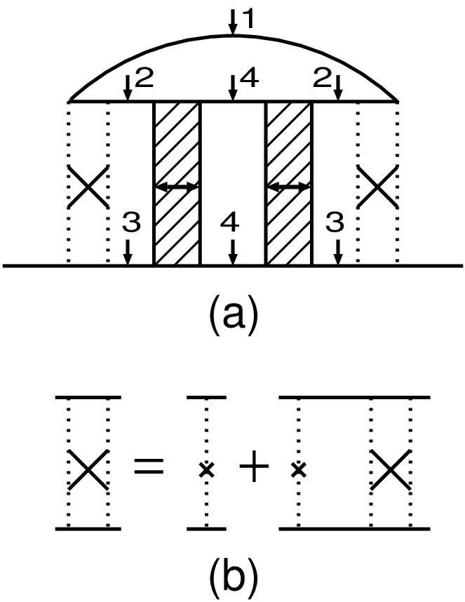
The vertex corrections to the response function are given by the functional derivative of the self-energy by the one-particle Green function. [31] These four-point interaction vertices are obtained by cutting the lines specified by the arrows in the self-energy in Fig. 2(a), which is equivalent to Fig. 1(a).
Refer to caption
Figure 2: (a) The self-energy correction is rewritten to obtain the vertex correction to the response function. The solid lines indicate the one-particle Green function [Eqs. (6)–(8)]. The meaning of the shaded square is the same as that in Fig. 1. The dotted square including a cross means the diffuson propagator. The arrow numbers indicate the corresponding vertex corrections. (b) Diffuson propagator. This is given by the ladder of the impurity scattering, which is represented by a single dotted line with a cross.

The arrow numbers indicate the corresponding vertex corrections. When we cut the solid lines with arrow numbers “1”, “2”, “3”, and “4”, we obtain the four-point interaction vertices corresponding to the Maki–Thompson (MT) term, the MT term corrected by the diffuson, the density of states (DOS) term, and the Aslamazov–Larkin (AL) term, respectively. These are written as “M​T​0MT0”, “M​TMT”, “D​O​SDOS”, and “A​LAL” below, respectively.

The four-point interaction vertex obtained in this way is called an irreducible four-point interaction vertex. The reducible four-point interaction vertex is obtained by the ladder-type summation of the irreducible vertex. As the number of rungs of the ladder increases, the exponent nn of 1/(kF​l)2​n1/(k_{F}l)^{2n} (the coefficient of the correction term) increases. Thus, we take account of only the lowest order of 1/(kF​l)21/(k_{F}l)^{2}. [32] This perturbation method is consistent with an approximation that the one-particle Green’s function [Eqs. (6)–(8)] does not include the weak localization effect, [29] and it is necessary to calculate the self-energy term in Sect. 3.2.2 [Fig. 4(a)] below because of this approximation.

3.2 Expressions of correction terms for linear absorption

3.2.1 Maki–Thompson terms

The diagrams of the MT terms are shown in Fig. 3.

Refer to caption
Figure 3: (a) Diagram of the conductivity corrected by the four-point interaction vertex, which is obtained by cutting the line “1” in Fig. 2(a) (σωM​T​0\sigma^{MT0}_{\omega}). (b) Diagram of the conductivity derived in the same way as in (a) by cutting the line “2” in Fig. 2(a) (σωM​T\sigma^{MT}_{\omega}). The dotted wavy line indicates the current vertex.

As derived in Appendix A.1, the expression for one of the MT terms [Fig. 3(a)] is written as

Re​σωM​T​0σ0=−3​3​τω​(4​π​kF​l)2​∫d​x​x​∫d​ϵ​∫d​ω′​Im​Qϵ,ω′,xM​T​0​(ω)\frac{{\rm Re}\sigma^{MT0}_{\omega}}{\sigma_{0}}=\frac{-3\sqrt{3\tau}}{\omega(4\pi k_{F}l)^{2}}\int dx\sqrt{x}\int d\epsilon\int d\omega^{\prime}{\rm Im}Q^{MT0}_{\epsilon,\omega^{\prime},x}(\omega) (17)

(x=D​q′2x=Dq^{\prime 2} with D=vF2​τ/3D=v_{F}^{2}\tau/3 being the diffusion constant and σ0=e2​ne​τ/m\sigma_{0}=e^{2}n_{e}\tau/m with ne=kF3/3​π2n_{e}=k_{F}^{3}/3\pi^{2}). Here,

Qϵ,ω′,xM​T​0​(ω)=∑i=0,1,2,3,42Γi(q′){Ctω′∑s=±s(Thϵ4𝒩i+++s+Thϵ3𝒩i++s−+Thϵ2𝒩i+s−−+Thϵ1𝒩is−−−)+∑s,s′=±ss′(Thϵ3Thϵ4𝒩i++ss′+Thϵ2Thϵ4𝒩i+s−s′)+𝒩i+++−+𝒩i−−−+}\begin{split}Q^{MT0}_{\epsilon,\omega^{\prime},x}(\omega)=&\sum_{i=0,1,2,3,4}2\Gamma_{i}(q^{\prime})\{C^{t}_{\omega^{\prime}}\sum_{s=\pm}s(T^{h}_{\epsilon_{4}}{\cal N}_{i}^{+++s}+T^{h}_{\epsilon_{3}}{\cal N}_{i}^{++s-}+T^{h}_{\epsilon_{2}}{\cal N}_{i}^{+s--}+T^{h}_{\epsilon_{1}}{\cal N}_{i}^{s---})\\ &+\sum_{s,s^{\prime}=\pm}ss^{\prime}(T^{h}_{\epsilon_{3}}T^{h}_{\epsilon_{4}}{\cal N}_{i}^{++ss^{\prime}}+T^{h}_{\epsilon_{2}}T^{h}_{\epsilon_{4}}{\cal N}_{i}^{+s-s^{\prime}})+{\cal N}_{i}^{+++-}+{\cal N}_{i}^{---+}\}\end{split} (18)

with Cωt=coth⁡(ω/2​T)C^{t}_{\omega}={\rm coth}(\omega/2T), Tϵh=tanh⁡(ϵ/2​T)T^{h}_{\epsilon}={\rm tanh}(\epsilon/2T), ϵ1=ϵ+(ω+ω′)/2\epsilon_{1}=\epsilon+(\omega+\omega^{\prime})/2, ϵ2=ϵ+(ω−ω′)/2\epsilon_{2}=\epsilon+(\omega-\omega^{\prime})/2, ϵ3=ϵ−(ω+ω′)/2\epsilon_{3}=\epsilon-(\omega+\omega^{\prime})/2, and ϵ4=ϵ−(ω−ω′)/2\epsilon_{4}=\epsilon-(\omega-\omega^{\prime})/2.

𝒩is1​s2​s3​s4=Tr⁡[(τ^0+s​τ^j​g^ϵ1s1​τ^j​g^ϵ2s2)​(τ^0+s​g^ϵ3s3​τ^j​g^ϵ4s4​τ^j)]2​(x+ζϵ1s1+ζϵ2s2)​(x+ζϵ3s3+ζϵ4s4){\cal N}_{i}^{s_{1}s_{2}s_{3}s_{4}}=\frac{{\rm Tr}[(\hat{\tau}_{0}+s\hat{\tau}_{j}\hat{g}^{s_{1}}_{\epsilon_{1}}\hat{\tau}_{j}\hat{g}^{s_{2}}_{\epsilon_{2}})(\hat{\tau}_{0}+s\hat{g}^{s_{3}}_{\epsilon_{3}}\hat{\tau}_{j}\hat{g}^{s_{4}}_{\epsilon_{4}}\hat{\tau}_{j})]}{2(x+\zeta^{s_{1}}_{\epsilon_{1}}+\zeta^{s_{2}}_{\epsilon_{2}})(x+\zeta^{s_{3}}_{\epsilon_{3}}+\zeta^{s_{4}}_{\epsilon_{4}})} (19)

for i=0,1,2,3i=0,1,2,3 [s={1(i=0,3)−1(i=1,2) and j={3(i=2,3)0(i=0,1)]\left[s=\left\{\begin{smallmatrix}1&(i=0,3)\\ -1&(i=1,2)\end{smallmatrix}\right.\text{ and }j=\left\{\begin{smallmatrix}3&(i=2,3)\\ 0&(i=0,1)\end{smallmatrix}\right.\right] and

𝒩4s1​s2​s3​s4=−Tr⁡[τ^1​g^ϵ1s1​τ^j​g^ϵ2s2​g^ϵ3s3​τ^j​g^ϵ4s4](x+ζϵ1s1+ζϵ2s2)​(x+ζϵ3s3+ζϵ4s4){\cal N}_{4}^{s_{1}s_{2}s_{3}s_{4}}=\frac{-{\rm Tr}[\hat{\tau}_{1}\hat{g}^{s_{1}}_{\epsilon_{1}}\hat{\tau}_{j}\hat{g}^{s_{2}}_{\epsilon_{2}}\hat{g}^{s_{3}}_{\epsilon_{3}}\hat{\tau}_{j}\hat{g}^{s_{4}}_{\epsilon_{4}}]}{(x+\zeta^{s_{1}}_{\epsilon_{1}}+\zeta^{s_{2}}_{\epsilon_{2}})(x+\zeta^{s_{3}}_{\epsilon_{3}}+\zeta^{s_{4}}_{\epsilon_{4}})} (20)

with g^ϵ±:=gϵ±​τ^0+fϵ±​τ^1\hat{g}_{\epsilon}^{\pm}:=g_{\epsilon}^{\pm}\hat{\tau}_{0}+f_{\epsilon}^{\pm}\hat{\tau}_{1} (gϵ±=−ϵ/ζ±ϵg_{\epsilon}^{\pm}=-\epsilon/\zeta^{\pm}_{\epsilon} and fϵ±=−Δ/ζ±ϵf_{\epsilon}^{\pm}=-\Delta/\zeta^{\pm}_{\epsilon}). Γi=0,1,2,3,4\Gamma_{i=0,1,2,3,4} represent the screened Coulomb interaction and the superconducting fluctuation [33] and are written as

(Γ3​(q)Γ2​(q)Γ4​(q))=1(1/p+χ2)​[1−(p+cq)​χ3]+4​(p+cq)​(χ′)2​((p+cq)​(1/p+χ2)/2−[1−(p+cq)χ3]/2−(p+cq)​χ′),\begin{pmatrix}\Gamma_{3}(q)\\ \Gamma_{2}(q)\\ \Gamma_{4}(q)\end{pmatrix}=\frac{1}{(1/p+\chi_{2})[1-(p+c_{q})\chi_{3}]+4(p+c_{q})(\chi^{\prime})^{2}}\begin{pmatrix}(p+c_{q})(1/p+\chi_{2})/2\\ -[1-(p+c_{q})\chi_{3}]/2\\ -(p+c_{q})\chi^{\prime}\end{pmatrix}, (21)
Γ0​(q)=p/21−p​χ0,\Gamma_{0}(q)=\frac{p/2}{1-p\chi_{0}}, (22)

and

Γ1​(q)=−1/21/p+χ1\Gamma_{1}(q)=\frac{-1/2}{1/p+\chi_{1}} (23)

with p:=(π​ρ0/2)​(gp​h2/ωE)p:=(\pi\rho_{0}/2)(g_{ph}^{2}/\omega_{E}) and cq:=(π​ρ0/2)​v\mib​qCc_{q}:=(\pi\rho_{0}/2)v^{C}_{\mib q} (ρ0:=m​kF/π2\rho_{0}:=mk_{F}/\pi^{2}).

χi=∑s=±s∫d​ϵ2​π​iTr[Tϵh​Xϵ+ω,ϵ+s​τ^i​(hi​τ^i+g^ϵ+ω+​τ^i​g^ϵs)2​α​(1−2​Xϵ+ω,ϵ+s)+Tϵ+ωh​Xϵ+ω,ϵs−​τ^i​(hi​τ^i+g^ϵ+ωs​τ^i​g^ϵ−)2​α​(1−2​Xϵ+ω,ϵs−)]−2πhi′′\chi_{i}=\sum_{s=\pm}s\int\frac{d\epsilon}{2\pi i}{\rm Tr}\left[\frac{T^{h}_{\epsilon}X_{\epsilon+\omega,\epsilon}^{+s}\hat{\tau}_{i}(h_{i}\hat{\tau}_{i}+\hat{g}^{+}_{\epsilon+\omega}\hat{\tau}_{i}\hat{g}^{s}_{\epsilon})}{2\alpha(1-2X_{\epsilon+\omega,\epsilon}^{+s})}+\frac{T^{h}_{\epsilon+\omega}X_{\epsilon+\omega,\epsilon}^{s-}\hat{\tau}_{i}(h_{i}\hat{\tau}_{i}+\hat{g}^{s}_{\epsilon+\omega}\hat{\tau}_{i}\hat{g}^{-}_{\epsilon})}{2\alpha(1-2X_{\epsilon+\omega,\epsilon}^{s-})}\right]-\frac{2}{\pi}h_{i}^{\prime\prime} (24)

for i=0,1,2,3i=0,1,2,3 [hi={1(i=0,3)−1(i=1,2) and hi′′={1(i=0,3)0(i=1,2)]\left[h_{i}=\left\{\begin{smallmatrix}1&(i=0,3)\\ -1&(i=1,2)\end{smallmatrix}\right.\text{ and }h^{\prime\prime}_{i}=\left\{\begin{smallmatrix}1&(i=0,3)\\ 0&(i=1,2)\end{smallmatrix}\right.\right], and

χ=′∑s=±s∫d​ϵ2​π​iTr[Tϵh​Xϵ+ω,ϵ+s​(−i​τ^2)​g^ϵ+ω+​τ^3​g^ϵs4​α​(1−2​Xϵ+ω,ϵ+s)+Tϵ+ωh​Xϵ+ω,ϵs−​(−i​τ^2)​g^ϵ+ωs​τ^3​g^ϵ−4​α​(1−2​Xϵ+ω,ϵs−)]\chi{{}^{\prime}}=\sum_{s=\pm}s\int\frac{d\epsilon}{2\pi i}{\rm Tr}\left[\frac{T^{h}_{\epsilon}X_{\epsilon+\omega,\epsilon}^{+s}(-i\hat{\tau}_{2})\hat{g}^{+}_{\epsilon+\omega}\hat{\tau}_{3}\hat{g}^{s}_{\epsilon}}{4\alpha(1-2X_{\epsilon+\omega,\epsilon}^{+s})}+\frac{T^{h}_{\epsilon+\omega}X_{\epsilon+\omega,\epsilon}^{s-}(-i\hat{\tau}_{2})\hat{g}^{s}_{\epsilon+\omega}\hat{\tau}_{3}\hat{g}^{-}_{\epsilon}}{4\alpha(1-2X_{\epsilon+\omega,\epsilon}^{s-})}\right] (25)

[τ^2=(0−ii0)\hat{\tau}_{2}=\left(\begin{smallmatrix}0&-i\\ i&0\end{smallmatrix}\right) ].

The expression of the real part of the conductivity corresponding to Fig. 3(b) (the MT term with an additional diffuson) is given by the following equation, the derivation of which is given in Appendix A.1:

Re​σωM​Tσ0=3​τω​(4​π​kF​l)2​∫d​x​x3/2​∫d​ϵ​∫d​ω′​Im​Qϵ,ω′,xM​T​(ω).\frac{{\rm Re}\sigma^{MT}_{\omega}}{\sigma_{0}}=\frac{\sqrt{3\tau}}{\omega(4\pi k_{F}l)^{2}}\int dxx^{3/2}\int d\epsilon\int d\omega^{\prime}{\rm Im}Q^{MT}_{\epsilon,\omega^{\prime},x}(\omega). (26)

Qϵ,ω′,xM​T​(ω)Q^{MT}_{\epsilon,\omega^{\prime},x}(\omega) is given by Eq. (18) with 𝒩{\cal N} replaced by the following ℳ{\cal M}:

ℳis1​s2​s3​s4=1(x+ζϵ1s1+ζϵ2s2)​(x+ζϵ3s3+ζϵ4s4)​(1x+ζϵ1s1+ζϵ3s3+1x+ζϵ2s2+ζϵ4s4)×12​Tr​[(τ^0+s​τ^j​g^ϵ1s1​τ^j​g^ϵ2s2)​(τ^0+s​g^ϵ3s3​τ^j​g^ϵ4s4​τ^j)+(τ^j′​g^ϵ1s1​τ^j′−s​g^ϵ2s2)​(s​g^ϵ3s3−τ^j′​g^ϵ4s4​τ^j′)]\begin{split}{\cal M}_{i}^{s_{1}s_{2}s_{3}s_{4}}=&\frac{1}{(x+\zeta^{s_{1}}_{\epsilon_{1}}+\zeta^{s_{2}}_{\epsilon_{2}})(x+\zeta^{s_{3}}_{\epsilon_{3}}+\zeta^{s_{4}}_{\epsilon_{4}})}\left(\frac{1}{x+\zeta^{s_{1}}_{\epsilon_{1}}+\zeta^{s_{3}}_{\epsilon_{3}}}+\frac{1}{x+\zeta^{s_{2}}_{\epsilon_{2}}+\zeta^{s_{4}}_{\epsilon_{4}}}\right)\\ &\times\frac{1}{2}{\rm Tr}[(\hat{\tau}_{0}+s\hat{\tau}_{j}\hat{g}^{s_{1}}_{\epsilon_{1}}\hat{\tau}_{j}\hat{g}^{s_{2}}_{\epsilon_{2}})(\hat{\tau}_{0}+s\hat{g}^{s_{3}}_{\epsilon_{3}}\hat{\tau}_{j}\hat{g}^{s_{4}}_{\epsilon_{4}}\hat{\tau}_{j})+(\hat{\tau}_{j^{\prime}}\hat{g}^{s_{1}}_{\epsilon_{1}}\hat{\tau}_{j^{\prime}}-s\hat{g}^{s_{2}}_{\epsilon_{2}})(s\hat{g}^{s_{3}}_{\epsilon_{3}}-\hat{\tau}_{j^{\prime}}\hat{g}^{s_{4}}_{\epsilon_{4}}\hat{\tau}_{j^{\prime}})]\end{split} (27)

for i=0,1,2,3i=0,1,2,3 [s={1(i=0,3)−1(i=1,2), j={3(i=2,3)0(i=0,1) and j′={0(i=2,3)3(i=0,1)]\left[s=\left\{\begin{smallmatrix}1&(i=0,3)\\ -1&(i=1,2)\end{smallmatrix}\right.,\text{ }j=\left\{\begin{smallmatrix}3&(i=2,3)\\ 0&(i=0,1)\end{smallmatrix}\right.\text{ and }j^{\prime}=\left\{\begin{smallmatrix}0&(i=2,3)\\ 3&(i=0,1)\end{smallmatrix}\right.\right] and

ℳ4s1​s2​s3​s4=Tr⁡[τ^1​(g^ϵ1s1​g^ϵ4s4−g^ϵ2s2​g^ϵ3s3−g^ϵ1s1​τ^j​g^ϵ2s2​g^ϵ3s3​τ^j​g^ϵ4s4)](x+ζϵ1s1+ζϵ2s2)​(x+ζϵ3s3+ζϵ4s4)​(1x+ζϵ1s1+ζϵ3s3+1x+ζϵ2s2+ζϵ4s4).{\cal M}_{4}^{s_{1}s_{2}s_{3}s_{4}}=\frac{{\rm Tr}[\hat{\tau}_{1}(\hat{g}^{s_{1}}_{\epsilon_{1}}\hat{g}^{s_{4}}_{\epsilon_{4}}-\hat{g}^{s_{2}}_{\epsilon_{2}}\hat{g}^{s_{3}}_{\epsilon_{3}}-\hat{g}^{s_{1}}_{\epsilon_{1}}\hat{\tau}_{j}\hat{g}^{s_{2}}_{\epsilon_{2}}\hat{g}^{s_{3}}_{\epsilon_{3}}\hat{\tau}_{j}\hat{g}^{s_{4}}_{\epsilon_{4}})]}{(x+\zeta^{s_{1}}_{\epsilon_{1}}+\zeta^{s_{2}}_{\epsilon_{2}})(x+\zeta^{s_{3}}_{\epsilon_{3}}+\zeta^{s_{4}}_{\epsilon_{4}})}\left(\frac{1}{x+\zeta^{s_{1}}_{\epsilon_{1}}+\zeta^{s_{3}}_{\epsilon_{3}}}+\frac{1}{x+\zeta^{s_{2}}_{\epsilon_{2}}+\zeta^{s_{4}}_{\epsilon_{4}}}\right). (28)

3.2.2 Density of states terms

The diagrams of the DOS terms are shown in Fig. 4.

Refer to caption
Figure 4: (a) Diagram of the conductivity corrected by the self-energy term (σωD​O​S​0\sigma^{DOS0}_{\omega}). (b) Diagram of the conductivity corrected by the four-point interaction vertex, which is obtained by cutting the line “3” in Fig. 2(a) (σωD​O​S\sigma^{DOS}_{\omega}).

As derived in Appendix A.2, the result of the self-energy term [Fig. 4(a)] is written as

Re​σωD​O​S​0σ0=−3​3​τω​(8​π​kF​l)2​∫d​x​x​∫d​ϵ​∫d​ω′​Im​Qϵ,ω′,xD​O​S​0​(ω)\frac{{\rm Re}\sigma^{DOS0}_{\omega}}{\sigma_{0}}=\frac{-3\sqrt{3\tau}}{\omega(8\pi k_{F}l)^{2}}\int dx\sqrt{x}\int d\epsilon\int d\omega^{\prime}{\rm Im}Q^{DOS0}_{\epsilon,\omega^{\prime},x}(\omega) (29)

with

QD​O​S​0ϵ,ω′,x(ω)=∑i=0,1,2,3,42{Ctω′[Γi(q′)−Γi∗(q′)]∑s=±s(Thϵ4𝒮i+++s+Thϵ1𝒮is​s​s−)+Γi(q′)(∑s,s′=±ss′Thϵ2Thϵ4𝒮i+s+s′+∑s=±sThϵ2Thϵ1𝒮i+s+−)−Γi∗(q′)∑s=±sThϵ1Thϵ2𝒮i−s−−},\begin{split}&Q^{DOS0}_{\epsilon,\omega^{\prime},x}(\omega)=\sum_{i=0,1,2,3,4}2\{C^{t}_{\omega^{\prime}}[\Gamma_{i}(q^{\prime})-\Gamma_{i}^{*}(q^{\prime})]\sum_{s=\pm}s(T^{h}_{\epsilon_{4}}{\cal S}_{i}^{+++s}+T^{h}_{\epsilon_{1}}{\cal S}_{i}^{sss-})\\ &+\Gamma_{i}(q^{\prime})(\sum_{s,s^{\prime}=\pm}ss^{\prime}T^{h}_{\epsilon_{2}}T^{h}_{\epsilon_{4}}{\cal S}_{i}^{+s+s^{\prime}}+\sum_{s=\pm}sT^{h}_{\epsilon_{2}}T^{h}_{\epsilon_{1}}{\cal S}_{i}^{+s+-})-\Gamma_{i}^{*}(q^{\prime})\sum_{s=\pm}sT^{h}_{\epsilon_{1}}T^{h}_{\epsilon_{2}}{\cal S}_{i}^{-s--}\},\end{split} (30)

where Γ∗\Gamma^{*} means the complex conjugate of Γ\Gamma. Here,

𝒮is1​s2​s3​s4=Tr⁡[s​τ^0+g^ϵ1s1​τ^j​g^ϵ2s2​τ^j−s​g^ϵ1s1​τ^3​g^ϵ1s3​τ^3+g^ϵ2s2​τ^j​g^ϵ1s3​τ^j+3​(s​g^ϵ1s1−τ^j′​g^ϵ2s2​τ^j′+s​g^ϵ1s3+g^ϵ1s1​τ^j​g^ϵ2s2​τ^j​g^ϵ1s3)​g^ϵ4s4]2​(x+ζϵ1s1+ζϵ2s2)​(x+ζϵ1s3+ζϵ2s2){\cal S}_{i}^{s_{1}s_{2}s_{3}s_{4}}=\frac{{\rm Tr}[s\hat{\tau}_{0}+\hat{g}^{s_{1}}_{\epsilon_{1}}\hat{\tau}_{j}\hat{g}^{s_{2}}_{\epsilon_{2}}\hat{\tau}_{j}-s\hat{g}^{s_{1}}_{\epsilon_{1}}\hat{\tau}_{3}\hat{g}^{s_{3}}_{\epsilon_{1}}\hat{\tau}_{3}+\hat{g}^{s_{2}}_{\epsilon_{2}}\hat{\tau}_{j}\hat{g}^{s_{3}}_{\epsilon_{1}}\hat{\tau}_{j}+3(s\hat{g}^{s_{1}}_{\epsilon_{1}}-\hat{\tau}_{j^{\prime}}\hat{g}^{s_{2}}_{\epsilon_{2}}\hat{\tau}_{j^{\prime}}+s\hat{g}^{s_{3}}_{\epsilon_{1}}+\hat{g}^{s_{1}}_{\epsilon_{1}}\hat{\tau}_{j}\hat{g}^{s_{2}}_{\epsilon_{2}}\hat{\tau}_{j}\hat{g}^{s_{3}}_{\epsilon_{1}})\hat{g}^{s_{4}}_{\epsilon_{4}}]}{2(x+\zeta^{s_{1}}_{\epsilon_{1}}+\zeta^{s_{2}}_{\epsilon_{2}})(x+\zeta^{s_{3}}_{\epsilon_{1}}+\zeta^{s_{2}}_{\epsilon_{2}})} (31)

for i=0,1,2,3i=0,1,2,3 [the values of ss, jj, and j′j^{\prime} are the same as those in ℳ{\cal M} below Eq. (27)] and

𝒮4s1​s2​s3​s4=−Tr⁡[τ^1​(g^ϵ1s1​τ^3​g^ϵ2s2​τ^3−g^ϵ2s2​τ^3​g^ϵ1s3​τ^3+3​g^ϵ2s2​g^ϵ4s4+3​g^ϵ1s1​τ^3​g^ϵ2s2​τ^3​g^ϵ1s3​g^ϵ4s4)](x+ζϵ1s1+ζϵ2s2)​(x+ζϵ1s3+ζϵ2s2).{\cal S}_{4}^{s_{1}s_{2}s_{3}s_{4}}=\frac{-{\rm Tr}[\hat{\tau}_{1}(\hat{g}^{s_{1}}_{\epsilon_{1}}\hat{\tau}_{3}\hat{g}^{s_{2}}_{\epsilon_{2}}\hat{\tau}_{3}-\hat{g}^{s_{2}}_{\epsilon_{2}}\hat{\tau}_{3}\hat{g}^{s_{3}}_{\epsilon_{1}}\hat{\tau}_{3}+3\hat{g}^{s_{2}}_{\epsilon_{2}}\hat{g}^{s_{4}}_{\epsilon_{4}}+3\hat{g}^{s_{1}}_{\epsilon_{1}}\hat{\tau}_{3}\hat{g}^{s_{2}}_{\epsilon_{2}}\hat{\tau}_{3}\hat{g}^{s_{3}}_{\epsilon_{1}}\hat{g}^{s_{4}}_{\epsilon_{4}})]}{(x+\zeta^{s_{1}}_{\epsilon_{1}}+\zeta^{s_{2}}_{\epsilon_{2}})(x+\zeta^{s_{3}}_{\epsilon_{1}}+\zeta^{s_{2}}_{\epsilon_{2}})}. (32)

The expression of the DOS term shown in Fig. 4(b) is given by the following equation:

Re​σωD​O​Sσ0=−3​τω​(4​π​kF​l)2​∫d​x​x3/2​∫d​ϵ​∫d​ω′​Im​Qϵ,ω′,xD​O​S​(ω).\frac{{\rm Re}\sigma^{DOS}_{\omega}}{\sigma_{0}}=\frac{-\sqrt{3\tau}}{\omega(4\pi k_{F}l)^{2}}\int dxx^{3/2}\int d\epsilon\int d\omega^{\prime}{\rm Im}Q^{DOS}_{\epsilon,\omega^{\prime},x}(\omega). (33)

Qϵ,ω′,xD​O​S​(ω)Q^{DOS}_{\epsilon,\omega^{\prime},x}(\omega) is given by Eq. (30) with 𝒮{\cal S} replaced by the following 𝒟{\cal D}:

𝒟is1​s2​s3​s4=Tr⁡[s​τ^0+g^ϵ1s1​τ^j​g^ϵ2s2​τ^j−s​g^ϵ1s1​τ^3​g^ϵ1s3​τ^3+g^ϵ2s2​τ^j​g^ϵ1s3​τ^j−(s​g^ϵ1s1−τ^j′​g^ϵ2s2​τ^j′+s​g^ϵ1s3+g^ϵ1s1​τ^j​g^ϵ2s2​τ^j​g^ϵ1s3)​g^ϵ4s4]2​(x+ζϵ1s1+ζϵ2s2)​(x+ζϵ1s3+ζϵ2s2)​(x+ζϵ4s4+ζϵ2s2){\cal D}_{i}^{s_{1}s_{2}s_{3}s_{4}}=\frac{{\rm Tr}[s\hat{\tau}_{0}+\hat{g}^{s_{1}}_{\epsilon_{1}}\hat{\tau}_{j}\hat{g}^{s_{2}}_{\epsilon_{2}}\hat{\tau}_{j}-s\hat{g}^{s_{1}}_{\epsilon_{1}}\hat{\tau}_{3}\hat{g}^{s_{3}}_{\epsilon_{1}}\hat{\tau}_{3}+\hat{g}^{s_{2}}_{\epsilon_{2}}\hat{\tau}_{j}\hat{g}^{s_{3}}_{\epsilon_{1}}\hat{\tau}_{j}-(s\hat{g}^{s_{1}}_{\epsilon_{1}}-\hat{\tau}_{j^{\prime}}\hat{g}^{s_{2}}_{\epsilon_{2}}\hat{\tau}_{j^{\prime}}+s\hat{g}^{s_{3}}_{\epsilon_{1}}+\hat{g}^{s_{1}}_{\epsilon_{1}}\hat{\tau}_{j}\hat{g}^{s_{2}}_{\epsilon_{2}}\hat{\tau}_{j}\hat{g}^{s_{3}}_{\epsilon_{1}})\hat{g}^{s_{4}}_{\epsilon_{4}}]}{2(x+\zeta^{s_{1}}_{\epsilon_{1}}+\zeta^{s_{2}}_{\epsilon_{2}})(x+\zeta^{s_{3}}_{\epsilon_{1}}+\zeta^{s_{2}}_{\epsilon_{2}})(x+\zeta^{s_{4}}_{\epsilon_{4}}+\zeta^{s_{2}}_{\epsilon_{2}})} (34)

for i=0,1,2,3i=0,1,2,3 (the values of ss, jj, and j′j^{\prime} are the same as those in the cases of ℳ{\cal M} and 𝒮{\cal S} above) and

𝒟4s1​s2​s3​s4=−Tr⁡[τ^1​(g^ϵ1s1​τ^3​g^ϵ2s2​τ^3−g^ϵ2s2​τ^3​g^ϵ1s3​τ^3−g^ϵ2s2​g^ϵ4s4−g^ϵ1s1​τ^3​g^ϵ2s2​τ^3​g^ϵ1s3​g^ϵ4s4)](x+ζϵ1s1+ζϵ2s2)​(x+ζϵ1s3+ζϵ2s2)​(x+ζϵ4s4+ζϵ2s2).{\cal D}_{4}^{s_{1}s_{2}s_{3}s_{4}}=\frac{-{\rm Tr}[\hat{\tau}_{1}(\hat{g}^{s_{1}}_{\epsilon_{1}}\hat{\tau}_{3}\hat{g}^{s_{2}}_{\epsilon_{2}}\hat{\tau}_{3}-\hat{g}^{s_{2}}_{\epsilon_{2}}\hat{\tau}_{3}\hat{g}^{s_{3}}_{\epsilon_{1}}\hat{\tau}_{3}-\hat{g}^{s_{2}}_{\epsilon_{2}}\hat{g}^{s_{4}}_{\epsilon_{4}}-\hat{g}^{s_{1}}_{\epsilon_{1}}\hat{\tau}_{3}\hat{g}^{s_{2}}_{\epsilon_{2}}\hat{\tau}_{3}\hat{g}^{s_{3}}_{\epsilon_{1}}\hat{g}^{s_{4}}_{\epsilon_{4}})]}{(x+\zeta^{s_{1}}_{\epsilon_{1}}+\zeta^{s_{2}}_{\epsilon_{2}})(x+\zeta^{s_{3}}_{\epsilon_{1}}+\zeta^{s_{2}}_{\epsilon_{2}})(x+\zeta^{s_{4}}_{\epsilon_{4}}+\zeta^{s_{2}}_{\epsilon_{2}})}. (35)

3.2.3 Aslamazov–Larkin term

The diagram of the AL term is shown in Fig. 5.

Refer to caption
Figure 5: Diagram of the conductivity corrected by the four-point interaction vertex obtained by cutting “4” lines in Fig. 2(a). σωA​L=σωA​L​1+σωA​L​2\sigma^{AL}_{\omega}=\sigma^{AL1}_{\omega}+\sigma^{AL2}_{\omega} with the left diagram (σωA​L​1\sigma^{AL1}_{\omega}) and the right diagram (σωA​L​2\sigma^{AL2}_{\omega}).

The result of the AL term (σωA​L=σωA​L​1+σωA​L​2\sigma^{AL}_{\omega}=\sigma^{AL1}_{\omega}+\sigma^{AL2}_{\omega}) is given by the following equation, the derivation of which is given in Appendix A.3:

Re​σωA​Lσ0=3​τ2​π3​ω​(kF​l)2​∫d​ω′​∫d​x​x3/2​Re​Qω′,xA​L​(ω)\frac{{\rm Re}\sigma^{AL}_{\omega}}{\sigma_{0}}=\frac{\sqrt{3\tau}}{2\pi^{3}\omega(k_{F}l)^{2}}\int d\omega^{\prime}\int dxx^{3/2}{\rm Re}Q^{AL}_{\omega^{\prime},x}(\omega) (36)

with

Qω′,xA​L​(ω)=∑i=3,2{Γ1(q−q′)[Ctω′Γi(q′)(𝒜(1)i,1)2+(Ctω−Ctω′)Γ∗i(q′)(𝒜(2)i,1)2−CtωΓ∗i(q′)𝒜(2)i,1𝒜(3)i,1]+Γi(q−q′)[Ctω′Γ1(q′)(𝒜(1)i,2)2+(Ctω−Ctω′)Γ∗1(q′)(𝒜(2)i,2)2−CtωΓ∗1(q′)𝒜(2)i,2𝒜(3)i,2]}+Γ1​(q−q′)​[2​Cω′t​Γ4​(q′)​𝒜2,1(1)​𝒜3,1(1)+2​(Cωt−Cω′t)​Γ4∗​(q′)​𝒜2,1(2)​𝒜3,1(2)−Cωt​Γ4∗​(q′)​(𝒜2,1(2)​𝒜3,1(3)+𝒜3,1(2)​𝒜2,1(3))]−Γ4​(q−q′)​[2​Cω′t​Γ1​(q′)​𝒜2,2(1)​𝒜3,2(1)+2​(Cωt−Cω′t)​Γ1∗​(q′)​𝒜2,2(2)​𝒜3,2(2)−Cωt​Γ1∗​(q′)​(𝒜2,2(2)​𝒜3,2(3)+𝒜3,2(2)​𝒜2,2(3))].\begin{split}Q^{AL}_{\omega^{\prime},x}(\omega)=&\sum_{i=3,2}\{\Gamma_{1}(q-q^{\prime})[C^{t}_{\omega^{\prime}}\Gamma_{i}(q^{\prime})({\cal A}^{(1)}_{i,1})^{2}+(C^{t}_{\omega}-C^{t}_{\omega^{\prime}})\Gamma^{*}_{i}(q^{\prime})({\cal A}^{(2)}_{i,1})^{2}-C^{t}_{\omega}\Gamma^{*}_{i}(q^{\prime}){\cal A}^{(2)}_{i,1}{\cal A}^{(3)}_{i,1}]\\ &+\Gamma_{i}(q-q^{\prime})[C^{t}_{\omega^{\prime}}\Gamma_{1}(q^{\prime})({\cal A}^{(1)}_{i,2})^{2}+(C^{t}_{\omega}-C^{t}_{\omega^{\prime}})\Gamma^{*}_{1}(q^{\prime})({\cal A}^{(2)}_{i,2})^{2}-C^{t}_{\omega}\Gamma^{*}_{1}(q^{\prime}){\cal A}^{(2)}_{i,2}{\cal A}^{(3)}_{i,2}]\}\\ &+\Gamma_{1}(q-q^{\prime})[2C^{t}_{\omega^{\prime}}\Gamma_{4}(q^{\prime}){\cal A}^{(1)}_{2,1}{\cal A}^{(1)}_{3,1}+2(C^{t}_{\omega}-C^{t}_{\omega^{\prime}})\Gamma^{*}_{4}(q^{\prime}){\cal A}^{(2)}_{2,1}{\cal A}^{(2)}_{3,1}-C^{t}_{\omega}\Gamma^{*}_{4}(q^{\prime})({\cal A}^{(2)}_{2,1}{\cal A}^{(3)}_{3,1}+{\cal A}^{(2)}_{3,1}{\cal A}^{(3)}_{2,1})]\\ &-\Gamma_{4}(q-q^{\prime})[2C^{t}_{\omega^{\prime}}\Gamma_{1}(q^{\prime}){\cal A}^{(1)}_{2,2}{\cal A}^{(1)}_{3,2}+2(C^{t}_{\omega}-C^{t}_{\omega^{\prime}})\Gamma^{*}_{1}(q^{\prime}){\cal A}^{(2)}_{2,2}{\cal A}^{(2)}_{3,2}-C^{t}_{\omega}\Gamma^{*}_{1}(q^{\prime})({\cal A}^{(2)}_{2,2}{\cal A}^{(3)}_{3,2}+{\cal A}^{(2)}_{3,2}{\cal A}^{(3)}_{2,2})].\end{split} (37)

Here,

𝒜i,j(1)=∑s=±s∫dϵ(Tϵhℒi,j+s++Tϵ+ω′hℒi,j+−s+Tϵ+ωhℒi,js−−),{\cal A}^{(1)}_{i,j}=\sum_{s=\pm}s\int d\epsilon(T^{h}_{\epsilon}{\cal L}_{i,j}^{+s+}+T^{h}_{\epsilon+\omega^{\prime}}{\cal L}_{i,j}^{+-s}+T^{h}_{\epsilon+\omega}{\cal L}_{i,j}^{s--}), (38)
𝒜i,j(2)=∑s=±s∫dϵ(Tϵ+ω′hℒi,j++s+Tϵhℒi,j+s−+Tϵ+ωhℒi,js−−),{\cal A}^{(2)}_{i,j}=\sum_{s=\pm}s\int d\epsilon(T^{h}_{\epsilon+\omega^{\prime}}{\cal L}_{i,j}^{++s}+T^{h}_{\epsilon}{\cal L}_{i,j}^{+s-}+T^{h}_{\epsilon+\omega}{\cal L}_{i,j}^{s--}), (39)

and

𝒜i,j(3)=∑s=±s∫dϵ(Tϵ+ω′hℒi,j++s+Tϵ+ωhℒi,js+−+Tϵhℒi,j−s−){\cal A}^{(3)}_{i,j}=\sum_{s=\pm}s\int d\epsilon(T^{h}_{\epsilon+\omega^{\prime}}{\cal L}_{i,j}^{++s}+T^{h}_{\epsilon+\omega}{\cal L}_{i,j}^{s+-}+T^{h}_{\epsilon}{\cal L}_{i,j}^{-s-}) (40)

with

ℒ2,js1​s2​s3=Tr⁡[τ^0−g^ϵ+ωs1​g^ϵs2−τ^l​g^ϵ+ωs1​τ^l​g^ϵ+ω′s3−τ^l′​g^ϵs2​τ^l′​g^ϵ+ω′s3]2​(x+ζϵ+ωs1+ζϵ+ω′s3)​(x+ζϵs2+ζϵ+ω′s3){\cal L}_{2,j}^{s_{1}s_{2}s_{3}}=\frac{{\rm Tr}[\hat{\tau}_{0}-\hat{g}^{s_{1}}_{\epsilon+\omega}\hat{g}^{s_{2}}_{\epsilon}-\hat{\tau}_{l}\hat{g}^{s_{1}}_{\epsilon+\omega}\hat{\tau}_{l}\hat{g}^{s_{3}}_{\epsilon+\omega^{\prime}}-\hat{\tau}_{l^{\prime}}\hat{g}^{s_{2}}_{\epsilon}\hat{\tau}_{l^{\prime}}\hat{g}^{s_{3}}_{\epsilon+\omega^{\prime}}]}{2(x+\zeta^{s_{1}}_{\epsilon+\omega}+\zeta^{s_{3}}_{\epsilon+\omega^{\prime}})(x+\zeta^{s_{2}}_{\epsilon}+\zeta^{s_{3}}_{\epsilon+\omega^{\prime}})} (41)

and

ℒ3,js1​s2​s3=Tr⁡[τ1^​(τ^0−g^ϵ+ωs1​g^ϵs2+τ^l​g^ϵ+ωs1​τ^l​g^ϵ+ω′s3+τ^l′​g^ϵs2​τ^l′​g^ϵ+ω′s3)]2​(x+ζϵ+ωs1+ζϵ+ω′s3)​(x+ζϵs2+ζϵ+ω′s3).{\cal L}_{3,j}^{s_{1}s_{2}s_{3}}=\frac{{\rm Tr}[\hat{\tau_{1}}(\hat{\tau}_{0}-\hat{g}^{s_{1}}_{\epsilon+\omega}\hat{g}^{s_{2}}_{\epsilon}+\hat{\tau}_{l}\hat{g}^{s_{1}}_{\epsilon+\omega}\hat{\tau}_{l}\hat{g}^{s_{3}}_{\epsilon+\omega^{\prime}}+\hat{\tau}_{l^{\prime}}\hat{g}^{s_{2}}_{\epsilon}\hat{\tau}_{l^{\prime}}\hat{g}^{s_{3}}_{\epsilon+\omega^{\prime}})]}{2(x+\zeta^{s_{1}}_{\epsilon+\omega}+\zeta^{s_{3}}_{\epsilon+\omega^{\prime}})(x+\zeta^{s_{2}}_{\epsilon}+\zeta^{s_{3}}_{\epsilon+\omega^{\prime}})}. (42)

(l,l′)=(0,3)(l,l^{\prime})=(0,3) and (3,0)(3,0) for j=1j=1 and 22, respectively. The result in the case of the normal state [14] is obtained by setting Δ=0\Delta=0 in the above equations.

3.2.4 Maximally crossed term

The maximally crossed (MC) term is the vertex correction, which does not include the screened Coulomb interaction and the superconducting fluctuation explicitly, but gives a weak localization correction to the conductivity by the coherent backscattering effect. [1, 10] (The contribution of this term to the one-particle spectrum vanishes and is not included in Figs. 1 and 2.) The diagram of this term is shown in Fig. 6(b).

Refer to caption
Figure 6: (a) Diagram of the conductivity corrected by the crossed impurity scattering at the lowest order. (b) Diagram of the conductivity corrected by the maximally crossed impurity scattering (the Cooperon term).

As derived in Appendix A.4, the linear absorption by the maximally crossed term is written as

Re​σωM​Cσ0=3​3​τ8​π​ω​(kF​l)2∫dxx∫dϵ(Tϵ+ωh−Tϵh)Re∑s=±sTr⁡[τ^0+g^ϵ+ω+​g^ϵs]2​(x+ζϵ+ω++ζϵs).\frac{{\rm Re}\sigma^{MC}_{\omega}}{\sigma_{0}}=\frac{3\sqrt{3\tau}}{8\pi\omega(k_{F}l)^{2}}\int dx\sqrt{x}\int d\epsilon(T^{h}_{\epsilon+\omega}-T^{h}_{\epsilon}){\rm Re}\sum_{s=\pm}s\frac{{\rm Tr}[\hat{\tau}_{0}+\hat{g}^{+}_{\epsilon+\omega}\hat{g}^{s}_{\epsilon}]}{2(x+\zeta_{\epsilon+\omega}^{+}+\zeta_{\epsilon}^{s})}. (43)

4 Results

4.1 Numerical calculations

In this section, we numerically evaluate Eqs. (17), (26), (29), (33), (36), and (43). The ranges of integrations over x=D​q2x=Dq^{2}, ϵ\epsilon, and ω′\omega^{\prime} in these equation are x<1/τx<1/\tau, |ϵ||\epsilon|, and |ω′|<1/τ|\omega^{\prime}|<1/\tau, in which the approximation Eq. (50) holds. (The low-energy properties are given by this range.) We make the variables symmetrical in advance, such as ϵ1​–​4\epsilon_{1\textendash 4} below Eq. (18). The superconducting gap at T=0T=0 is taken to be the unit of energy (Δ0=1\Delta_{0}=1), and the electron–phonon coupling pp is determined by the gap equation. cqc_{q} (=π​ωp2​τ/2​D​q2≫p=\pi\omega_{p}^{2}\tau/2Dq^{2}\gg p with ωp=4​π​ne​e2/m\omega_{p}=\sqrt{4\pi n_{e}e^{2}/m} the plasma frequency) in the denominator and the numerator of Γ3,2,4​(q)\Gamma_{3,2,4}(q) cancel out each other as in Eqs. (45)–(47) in Ref. 25. (The effective interaction becomes independent of e2e^{2}. [34]) The relation between α=1/2​τ\alpha=1/2\tau and kF​lk_{F}l is fixed to kF​l/2​τ=EF=300​Δ0k_{F}l/2\tau=E_{F}=300\Delta_{0}, where EFE_{F} is the Fermi energy.

The calculated results of Γi​(q)\Gamma_{i}(q) at T=0T=0 are given in Ref. 25, in which it is shown that terms including the Coulomb interaction (Γ3,2,4\Gamma_{3,2,4}) are larger than other terms (Γ0,1\Gamma_{0,1}). In the case of the absorption spectrum, it can also be shown that terms including the Coulomb interaction predominantly contribute to the correction term. We will not show correction terms decomposed for each vertex (Γi\Gamma_{i}) explicitly below.

The dependence of Re​σω/σ0{\rm Re}\sigma_{\omega}/\sigma_{0} on ω\omega for several values of T/TcT/T_{c} is shown in Fig. 7.

Refer to caption
Figure 7: Dependence of Re​σω/σ0{\rm Re}\sigma_{\omega}/\sigma_{0} on ω\omega for kF​l=2.5k_{F}l=2.5. The numerical values on the left of lines are the values of T/TcT/T_{c}. The dotted thin lines represent c0×Re​σω(0)/σ0c_{0}\times{\rm Re}\sigma^{(0)}_{\omega}/\sigma_{0}. c0c_{0} is a constant with its value indicated as (0)×c0(0)\times c_{0}.

Here, σω=σω(0)+σωvc\sigma_{\omega}=\sigma^{(0)}_{\omega}+\sigma^{\rm vc}_{\omega} with σωvc=σωM​T​0+σωM​T+σωD​O​S​0+σωD​O​S+σωA​L+σωM​C\sigma^{\rm vc}_{\omega}=\sigma^{MT0}_{\omega}+\sigma^{MT}_{\omega}+\sigma^{DOS0}_{\omega}+\sigma^{DOS}_{\omega}+\sigma^{AL}_{\omega}+\sigma^{MC}_{\omega} [Re​σω=Re​σω(0)​(1+Re​σωvc/Re​σω(0)){\rm Re}\sigma_{\omega}={\rm Re}\sigma_{\omega}^{(0)}\left(1+{\rm Re}\sigma^{\rm vc}_{\omega}/{\rm Re}\sigma_{\omega}^{(0)}\right)]. Re​σω(0){\rm Re}\sigma^{(0)}_{\omega} is the real part of the conductivity given by the MB theory (i.e., the linear absorption without vertex corrections) and is written as

Re​σω(0)σ0=−12​ω∫dϵ(Tϵ+ωh−Tϵh)Re∑s=±s12Tr[g^ϵ+ω+g^ϵs].\frac{{\rm Re}\sigma^{(0)}_{\omega}}{\sigma_{0}}=\frac{-1}{2\omega}\int d\epsilon(T^{h}_{\epsilon+\omega}-T^{h}_{\epsilon}){\rm Re}\sum_{s=\pm}s\frac{1}{2}{\rm Tr}[\hat{g}^{+}_{\epsilon+\omega}\hat{g}^{s}_{\epsilon}]. (44)

The comparison of Re​σω/σ0{\rm Re}\sigma_{\omega}/\sigma_{0} with the MB formula Re​σω(0)/σ0{\rm Re}\sigma^{(0)}_{\omega}/\sigma_{0} is shown in Fig. 7. In this figure, (0)×c0(0)\times c_{0} represents the result of c0×Re​σω(0)/σ0c_{0}\times{\rm Re}\sigma^{(0)}_{\omega}/\sigma_{0}. c0c_{0} is chosen such that c0×Re​σω(0)/σ0c_{0}\times{\rm Re}\sigma^{(0)}_{\omega}/\sigma_{0} overlaps Re​σω/σ0{\rm Re}\sigma_{\omega}/\sigma_{0} in the range of ω⪅2​Δ\omega\lessapprox 2\Delta. This result shows that Re​σω/σ0{\rm Re}\sigma_{\omega}/\sigma_{0} is not proportional to the MB conductivity. The suppression of the conductivity by vertex corrections is larger at ω>2​Δ\omega>2\Delta than at ω<2​Δ\omega<2\Delta for low temperatures. As a result, the excitations below 2​Δ2\Delta (i.e., thermal excitations) seem to be relatively enhanced as compared with the behavior of the MB conductivity.

The ratio of vertex corrections to the MB conductivity, Re​σωvc/Re​σω(0){\rm Re}\sigma^{\rm vc}_{\omega}/{\rm Re}\sigma^{(0)}_{\omega}, is shown in Fig. 8.

Refer to caption
Refer to caption
Figure 8: (a) Ratio of the vertex correction to the MB conductivity, Re​σωvc/Re​σω(0){\rm Re}\sigma^{\rm vc}_{\omega}/{\rm Re}\sigma^{(0)}_{\omega}, for kF​l=2.5k_{F}l=2.5. The numerical values on the left of lines represent the values of T/TcT/T_{c}. (b) Re​σωvc/Re​σω(0){\rm Re}\sigma^{\rm vc}_{\omega}/{\rm Re}\sigma^{(0)}_{\omega} for several values of kF​lk_{F}l. The numerical values indicate the values of kF​lk_{F}l and T/TcT/T_{c} (kF​l=2.5k_{F}l=2.5, 3.53.5, and 5.05.0, and T/Tc=0.65T/T_{c}=0.65 and 1.11.1).

Figure 8(a) shows that the difference in Re​σωvc/Re​σω(0){\rm Re}\sigma^{\rm vc}_{\omega}/{\rm Re}\sigma^{(0)}_{\omega} between ω>2​Δ\omega>2\Delta and ω<2​Δ\omega<2\Delta becomes significant at low temperatures. The suppression of Re​σω{\rm Re}\sigma_{\omega} by vertex corrections is larger (smaller) than that in the normal state (T/Tc=1.1T/T_{c}=1.1) for ω>2​Δ\omega>2\Delta (ω<2​Δ\omega<2\Delta). The vertex correction is less effective for the thermal excitation (ω<2​Δ\omega<2\Delta). Figure 8(b) shows that the absolute value of Re​σωvc{\rm Re}\sigma^{\rm vc}_{\omega} is roughly proportional to 1/(kF​l)21/(k_{F}l)^{2}, as expected from the analytical expressions in the previous section. There also exists a difference between ω>2​Δ\omega>2\Delta and ω<2​Δ\omega<2\Delta for other values of kF​lk_{F}l, which is similar to the case of kF​l=2.5k_{F}l=2.5.

The components of Re​σωvc/σ0{\rm Re}\sigma^{\rm vc}_{\omega}/\sigma_{0} are shown in Fig. 9.

Refer to caption
Refer to caption
Refer to caption
Refer to caption
Refer to caption
Refer to caption
Figure 9: Components of Re​σωvc/σ0{\rm Re}\sigma^{\rm vc}_{\omega}/\sigma_{0} for kF​l=2.5k_{F}l=2.5. The numerical values on the left of lines are the values of T/TcT/T_{c}. The thin solid lines show the Mattis–Bardeen formula at T/Tc=0.65T/T_{c}=0.65 with a constant value multiplied (c0×Re​σω(0)/σ0c_{0}\times{\rm Re}\sigma^{(0)}_{\omega}/\sigma_{0}). (a) Re​σωM​T/σ0{\rm Re}\sigma^{MT}_{\omega}/\sigma_{0}. c0=−0.23c_{0}=-0.23. (b) Re​σωM​T​0/σ0{\rm Re}\sigma^{MT0}_{\omega}/\sigma_{0}. c0=0.42c_{0}=0.42. (c) Re​σωD​O​S/σ0{\rm Re}\sigma^{DOS}_{\omega}/\sigma_{0}. c0=0.7c_{0}=0.7. (d) Re​σωD​O​S​0/σ0{\rm Re}\sigma^{DOS0}_{\omega}/\sigma_{0}. c0=−0.4c_{0}=-0.4. (e) Re​σωA​L/σ0{\rm Re}\sigma^{AL}_{\omega}/\sigma_{0}. (f) Re​σωM​C/σ0{\rm Re}\sigma^{MC}_{\omega}/\sigma_{0}. c0=−0.25c_{0}=-0.25.

Figure 9 shows that Re​σωM​T,D​O​S​0,M​C/σ0{\rm Re}\sigma^{MT,DOS0,MC}_{\omega}/\sigma_{0} (Re​σωM​T​0,D​O​S,A​L/σ0{\rm Re}\sigma^{MT0,DOS,AL}_{\omega}/\sigma_{0}) takes a negative (positive) value. These vertex corrections are seemingly proportional to the MB conductivity. The comparison between vertex corrections and c0×Re​σω(0)/σ0c_{0}\times{\rm Re}\sigma^{(0)}_{\omega}/\sigma_{0} shows that this is not the case. Here, c0c_{0} is chosen in the same way as in Fig. 7. In the cases of Re​σωM​T,M​T​0,D​O​S,D​O​S​0{\rm Re}\sigma^{MT,MT0,DOS,DOS0}_{\omega}, the deviations from the MB conductivity show a similar ω\omega-dependence with each other. When we choose c0c_{0} so that c0×Re​σω(0)/σ0c_{0}\times{\rm Re}\sigma^{(0)}_{\omega}/\sigma_{0} overlaps Re​σωM​T,M​T​0,D​O​S,D​O​S​0{\rm Re}\sigma^{MT,MT0,DOS,DOS0}_{\omega} around ω⪅2​Δ\omega\lessapprox 2\Delta, each of |Re​σωM​T,M​T​0,D​O​S,D​O​S​0||{\rm Re}\sigma^{MT,MT0,DOS,DOS0}_{\omega}| takes values larger than |c0×Re​σω(0)/σ0||c_{0}\times{\rm Re}\sigma^{(0)}_{\omega}/\sigma_{0}| for ω>2​Δ\omega>2\Delta. This indicates that these four terms give larger corrections in Re​σω{\rm Re}\sigma_{\omega} for ω>2​Δ\omega>2\Delta than for ω<2​Δ\omega<2\Delta. The maximally crossed term shows an opposite tendency. The correction by the thermal excitation is larger than that by the excitation above 2​Δ2\Delta in the case of |Re​σωM​C||{\rm Re}\sigma^{MC}_{\omega}|. The AL term is smaller than other terms and negligible in the superconducting state, although Re​σωA​L{\rm Re}\sigma^{AL}_{\omega} in the normal state is enhanced for small ω\omega by the superconducting fluctuation near TcT_{c}. This smallness of the AL term originates from the fact that one of two fluctuation modes is the amplitude mode (Γ1\Gamma_{1}), as shown in Eq. (37). Note that Γ1\Gamma_{1} does not include the Coulomb interaction effect.

The ratios of components of vertex corrections to the MB conductivity are shown in Fig. 10.

Refer to caption
Refer to caption
Figure 10: Ratio Re​σωxx/Re​σω(0){\rm Re}\sigma^{\rm xx}_{\omega}/{\rm Re}\sigma^{(0)}_{\omega} for kF​l=2.5k_{F}l=2.5. Here, xx=M​T​0{\rm xx}=MT0, M​TMT, D​O​S​0DOS0, D​O​SDOS, A​LAL, or M​CMC as indicated in the figure. (a) T/Tc=0.45T/T_{c}=0.45 in the superconducting state. (b) T/Tc=1.1T/T_{c}=1.1 in the normal state.

The relationship between the sizes of vertex corrections in the superconducting state is similar to that in the normal state. For T/Tc=0.45T/T_{c}=0.45, the absolute values of the MT and DOS terms are smaller for ω<2​Δ\omega<2\Delta than for ω>2​Δ\omega>2\Delta, and show a variation around ω≃2​Δ\omega\simeq 2\Delta. The comparison of the absolute values between vertex corrections shows that Re​σωD​O​S​0{\rm Re}\sigma^{DOS0}_{\omega} gives a predominant contribution in Re​σω{\rm Re}\sigma_{\omega}, although there is a cancellation among vertex corrections. Thus, the difference in Re​σωD​O​S​0{\rm Re}\sigma^{DOS0}_{\omega} between ω<2​Δ\omega<2\Delta and ω>2​Δ\omega>2\Delta mainly leads to the deviation of Re​σω{\rm Re}\sigma_{\omega} from the MB-like behavior. For T/Tc=1.1T/T_{c}=1.1, Re​σωD​O​S​0{\rm Re}\sigma^{DOS0}_{\omega} is suppressed at small values of ω\omega, which causes a suppression of Re​σω{\rm Re}\sigma_{\omega} at low frequencies, as shown in Fig. 7.

4.2 Origin of the variation of the correction term around ω=2​Δ\omega=2\Delta

In this subsection, we show that the variation of the ratio Re​σωvc/Re​σω(0){\rm Re}\sigma^{\rm vc}_{\omega}/{\rm Re}\sigma^{(0)}_{\omega} around ω≃2​Δ\omega\simeq 2\Delta is related to the correction to the one-particle spectrum. Equation (44) is rewritten as Re​σω(0)/σ0=(Re​σω(0)​a+Re​σω(0)​b)/σ0{\rm Re}\sigma^{(0)}_{\omega}/\sigma_{0}=({\rm Re}\sigma^{(0)a}_{\omega}+{\rm Re}\sigma^{(0)b}_{\omega})/\sigma_{0} with Re​σω(0)​a/σ0=∫Δ+ω/2∞d​ϵ​hϵ,ω{\rm Re}\sigma^{(0)a}_{\omega}/\sigma_{0}=\int_{\Delta+\omega/2}^{\infty}d\epsilon h_{\epsilon,\omega} and Reσω(0)​b/σ0=−∫0ω/2−Δdϵθ(ω−2Δ)hϵ,ω{\rm Re}\sigma^{(0)b}_{\omega}/\sigma_{0}=-\int_{0}^{\omega/2-\Delta}d\epsilon\theta(\omega-2\Delta)h_{\epsilon,\omega} for ω>0\omega>0. Here, hϵ,ω=(Tϵ+ω/2h−Tϵ−ω/2h)​Tr​[Im​g^ϵ+ω/2+​Im​g^ϵ−ω/2+]/ωh_{\epsilon,\omega}=(T^{h}_{\epsilon+\omega/2}-T^{h}_{\epsilon-\omega/2}){\rm Tr}[{\rm Im}\hat{g}^{+}_{\epsilon+\omega/2}{\rm Im}\hat{g}^{+}_{\epsilon-\omega/2}]/\omega. Re​σω(0)​a{\rm Re}\sigma_{\omega}^{(0)a} is a decreasing function with respect to ω\omega and Re​σω(0)​b{\rm Re}\sigma_{\omega}^{(0)b} takes finite values only for ω>2​Δ\omega>2\Delta. The weak localization effect on the one-particle spectrum is approximately taken into account as Im​g^ϵ+×[1−(1−s′​(|ϵ|−Δ)​τ)/(kF​l)2]=:Im​g′^ϵ+{\rm Im}\hat{g}^{+}_{\epsilon}\times[1-(1-s^{\prime}\sqrt{(|\epsilon|-\Delta)\tau})/(k_{F}l)^{2}]=:{\rm Im}\hat{g^{\prime}}^{+}_{\epsilon}. s′=+s^{\prime}=+ (−)(-) means that the suppression of the density of states is large close to (apart from) the gap edge. Here, the case of s′=−s^{\prime}=- is used for comparison and does not correspond to the real system. We calculate the conductivity including this effect (Re​σω′=Re​σωa′+Re​σωb′{\rm Re}\sigma^{\prime}_{\omega}={\rm Re}\sigma^{{}^{\prime}a}_{\omega}+{\rm Re}\sigma^{{}^{\prime}b}_{\omega}) by replacing g^ϵ+\hat{g}^{+}_{\epsilon} by g′^ϵ+\hat{g^{\prime}}^{+}_{\epsilon} in the above hϵ,ωh_{\epsilon,\omega}. The correction part of the conductivity Re​σω′/Re​σω(0)−1{\rm Re}\sigma^{\prime}_{\omega}/{\rm Re}\sigma^{(0)}_{\omega}-1 is shown in Fig. 11.

Refer to caption
Figure 11: Correction part of the conductivity, Reσ′ω/Reσ(0)ω−1{\rm Re}\sigma^{{}^{\prime}}_{\omega}/{\rm Re}\sigma^{(0)}_{\omega}-1, induced by the suppression of the density of states. The numerical values indicate temperatures (T/TcT/T_{c}). The signs (±)(\pm) correspond to s′=±s^{\prime}=\pm in the main text.

The large variation of Reσ′ω/Reσ(0)ω−1{\rm Re}\sigma^{{}^{\prime}}_{\omega}/{\rm Re}\sigma^{(0)}_{\omega}-1 occurs around ω≃2​Δ\omega\simeq 2\Delta with the same (opposite) tendency for s′=+s^{\prime}=+ (−)(-) as that of Re​σωvc/Re​σω(0){\rm Re}\sigma^{\rm vc}_{\omega}/{\rm Re}\sigma^{(0)}_{\omega}.

In Re​σωa′{\rm Re}\sigma^{{}^{\prime}a}_{\omega}, which is given by the thermal excitations, ϵ+ω/2≃3​Δ\epsilon+\omega/2\simeq 3\Delta and ϵ−ω/2≃Δ\epsilon-\omega/2\simeq\Delta for ω≃2​Δ\omega\simeq 2\Delta (the contribution from ϵ≃Δ+ω/2\epsilon\simeq\Delta+\omega/2 is large in the integration at low temperatures), and then only Im​g′^ϵ−ω/2+{\rm Im}\hat{g^{\prime}}^{+}_{\epsilon-\omega/2} is put on the gap edge. On the other hand, in Re​σωb′{\rm Re}\sigma^{{}^{\prime}b}_{\omega}, which is given by excitations across the gap with ω≳2​Δ\omega\gtrsim 2\Delta, ϵ+ω/2≃Δ\epsilon+\omega/2\simeq\Delta and ϵ−ω/2≃−Δ\epsilon-\omega/2\simeq-\Delta for ω≃2​Δ\omega\simeq 2\Delta, and then both Im​g′^ϵ±ω/2+{\rm Im}\hat{g^{\prime}}^{+}_{\epsilon\pm\omega/2} are put on the gap edge. Thus, Re​σωb′{\rm Re}\sigma^{{}^{\prime}b}_{\omega} is more sensitive to the values of the density of states near the gap edge than Re​σωa′{\rm Re}\sigma^{{}^{\prime}a}_{\omega} in the case of ω≃2​Δ\omega\simeq 2\Delta. When the suppression of the density of states is larger near the gap edge than apart from the gap edge (corresponding to the case of s′=+s^{\prime}=+), the correction part of |Re​σωb′||{\rm Re}\sigma^{{}^{\prime}b}_{\omega}| for ω≳2​Δ\omega\gtrsim 2\Delta is larger than that of |Re​σωa′||{\rm Re}\sigma^{{}^{\prime}a}_{\omega}| for ω≲2​Δ\omega\lesssim 2\Delta. This leads to the negative slope of Re​σω′/Re​σω(0)−1{\rm Re}\sigma^{\prime}_{\omega}/{\rm Re}\sigma^{(0)}_{\omega}-1 around ω≃2​Δ\omega\simeq 2\Delta, as shown in Fig. 11.

5 Summary and Discussion

In this study, we calculated the weak localization correction to the linear absorption of three-dimensional s-wave superconductors. This correction is caused by the coherent backscattering and the interaction effect (Coulomb interaction and superconducting fluctuations) enhanced by the diffusion term. Numerical calculations show that the correction effect is greater on the excitations across the gap (ω>2​Δ\omega>2\Delta) than on the thermal excitations (ω<2​Δ\omega<2\Delta). This tendency is shown to be related to the weak localization correction to the one-particle spectrum. The latter is known as the Altshuler–Aronov effect, which was confirmed in experiments [35, 36].

We showed that the weak localization effect can be made clear by taking the ratio of the correction term to the MB formula. The dependence of this ratio on the frequency shows a large variation near ω≃2​Δ\omega\simeq 2\Delta. This variation indicates that the correction term relatively enhances the absorption by the thermal excitations as compared with that by the excitations across the gap and blurs the absorption edge in the spectrum. The experimental result in a strongly disordered system shows a qualitatively similar tendency. [20] The quantitative result is not explained by our calculation because this system is outside the range of the weak localization.

Even in the case of less disordered systems, by taking the ratio of the absorption spectrum to the MB formula, the weak localization effect should be visible as a variation of this ratio around ω≃2​Δ\omega\simeq 2\Delta. We consider that this ratio can be used as a sign of the weak localization.

In order to deal with a more disordered system (i.e., outside the weak localization regime) such as some experiments, [20, 21, 22] the following should be considered theoretically as future issues. Since the calculations in this paper are based on the perturbation theory, one way to improve the calculation is to take account of higher-order terms. This is needed when we consider the metal-insulator transition. As another possibility, it is conceivable to change the treatment of the impurity scattering, for example, by considering an inhomogeneous case. [23, 37] In this study, we considered a homogeneously disordered system, but it is meaningful to see how the Coulomb interaction (a predominant factor in the weak localization effect) is incorporated in the case of inhomogeneous systems. [38]

Acknowledgment

The numerical computation in this work was carried out at the Yukawa Institute Computer Facility.

Appendix A Derivation of Correction Terms for Linear Absorption

In this Appendix, we give a detailed derivation of the results shown in Sect. 3.2. We obtain expressions of correction terms Eqs. (17), (26), (29), (33), (36), and (43) by calculating Eqs. (3)–(5) with the use of Eqs. (6)–(16). The calculation is performed by expanding ei​S′e^{iS^{\prime}} in accordance with Figs. 3–6, and we incorporate the effects of interactions (i.e., the screened Coulomb interaction, superconducting fluctuation, and scattering by impurities) in accordance with Fig. 1. In the following subsections, we show the equations obtained by this process.

A.1 Maki–Thompson term

The real part of the conductivity shown in Fig. 3(a) is written as

Re​σωM​T​0=e22​ω​N3∑\mib​q′∫d​ω′2​π​i∫d​ϵ2​π​iIm{(π​ρ02)−1×∑i=0,1,2,3,4(∑𝒮1Cω′t​[Γi​(q′)−Γi∗​(q′)]+∑𝒮2Γi​(q′)+∑𝒮3Γi∗​(q′))×1N3∑\mib​kTr[I^s4,b′ϵ+ω′G^k+q′s4vk+q′G^k+q+q′s1I^s1,aϵ+ω+ω′Y^iI^s2,a′ϵ+ωG^k+qs2vkG^ks3I^s3,bϵY^′i]}.\begin{split}{\rm Re}\sigma^{MT0}_{\omega}=&\frac{e^{2}}{2\omega N^{3}}\sum_{\mib q^{\prime}}\int\frac{d\omega^{\prime}}{2\pi i}\int\frac{d\epsilon}{2\pi i}{\rm Im}\Bigl\{\left(\frac{\pi\rho_{0}}{2}\right)^{-1}\\ &\times\sum_{i=0,1,2,3,4}\left(\sum_{{\cal S}_{1}}C^{t}_{\omega^{\prime}}[\Gamma_{i}(q^{\prime})-\Gamma^{*}_{i}(q^{\prime})]+\sum_{{\cal S}_{2}}\Gamma_{i}(q^{\prime})+\sum_{{\cal S}_{3}}\Gamma^{*}_{i}(q^{\prime})\right)\\ &\times\frac{1}{N^{3}}\sum_{\mib k}{\rm Tr}[\hat{I}^{s_{4},b^{\prime}}_{\epsilon+\omega^{\prime}}\hat{G}_{k+q^{\prime}}^{s_{4}}v_{k+q^{\prime}}\hat{G}_{k+q+q^{\prime}}^{s_{1}}\hat{I}^{s_{1},a}_{\epsilon+\omega+\omega^{\prime}}\hat{Y}_{i}\hat{I}^{s_{2},a^{\prime}}_{\epsilon+\omega}\hat{G}_{k+q}^{s_{2}}v_{k}\hat{G}_{k}^{s_{3}}\hat{I}^{s_{3},b}_{\epsilon}\hat{Y}^{\prime}_{i}]\Bigr\}.\end{split} (45)

Γi=0,1,2,3,4\Gamma_{i=0,1,2,3,4} indicate the interaction effects [Eqs. (21)–(23)], and the derivation of these equations is given in Ref. 25. ∑𝒮1,2,3\sum_{{\cal S}_{1,2,3}} indicate the summations taken over (s1,s2,s3,s4)(s_{1},s_{2},s_{3},s_{4}) with

(s1,s2,s3,s4)={(+,+,+,K),(+,+,K,−),(+,K,−,−),(K,−,−,−)for ​𝒮1(+,+,K,K),(+,K,−,K),(+,+,+,−),(−,−,−,+)for ​𝒮2(K,+,K,−),(K,K,−,−),(+,−,−,−),(−,+,+,+)for ​𝒮3.(s_{1},s_{2},s_{3},s_{4})=\left\{\begin{matrix}(+,+,+,K),(+,+,K,-),(+,K,-,-),(K,-,-,-)&\text{for }{\cal S}_{1}\\ (+,+,K,K),(+,K,-,K),(+,+,+,-),(-,-,-,+)&\text{for }{\cal S}_{2}\\ (K,+,K,-),(K,K,-,-),(+,-,-,-),(-,+,+,+)&\text{for }{\cal S}_{3}.\end{matrix}\right. (46)

(I^)​(I^′)(\hat{I})(\hat{I}^{\prime}) represents the vertex correction by the impurity scattering, and it is written as

(I^ϵs1,x)​(I^ϵ−ω′s2,x′)=(τ^0)​(τ^0)+ni​u2N3​∑\mib​k(τ^3​G^ks1)​(G^k−q′s2​τ^3)+(ni​u2N3)2​∑\mib​k,\mib​k′(τ^3​G^ks1​τ^3​G^k′s1)​(G^k′−q′s2​τ^3​G^k−q′s2​τ^3)+⋯(\hat{I}^{s_{1},x}_{\epsilon})(\hat{I}^{s_{2},x^{\prime}}_{\epsilon-\omega^{\prime}})=(\hat{\tau}_{0})(\hat{\tau}_{0})+\frac{n_{i}u^{2}}{N^{3}}\sum_{\mib k}(\hat{\tau}_{3}\hat{G}_{k}^{s_{1}})(\hat{G}_{k-q^{\prime}}^{s_{2}}\hat{\tau}_{3})+\left(\frac{n_{i}u^{2}}{N^{3}}\right)^{2}\sum_{\mib k,\mib k^{\prime}}(\hat{\tau}_{3}\hat{G}_{k}^{s_{1}}\hat{\tau}_{3}\hat{G}_{k^{\prime}}^{s_{1}})(\hat{G}_{k^{\prime}-q^{\prime}}^{s_{2}}\hat{\tau}_{3}\hat{G}_{k-q^{\prime}}^{s_{2}}\hat{\tau}_{3})+\cdots (47)

(x=a,bx=a,b). (^)​(^)(\hat{\;\;})(\hat{\;\;}) represents a combination of matrices and does not mean a product of matrices [(A^)​(B^)≠A^​B^(\hat{A})(\hat{B})\neq\hat{A}\hat{B}]. The summation taken over \mib​k\mib k results in the following expression:

(I^ϵs1,x)​(I^ϵ−ω′s2,x′)=(τ^0)​(τ^0)+Xϵ,ϵ−ω′s1,s21−2​Xϵ,ϵ−ω′s1,s2​[(τ^3​g^ϵs1)​(g^ϵ−ω′s2​τ^3)+(τ^0)​(τ^0)](\hat{I}^{s_{1},x}_{\epsilon})(\hat{I}^{s_{2},x^{\prime}}_{\epsilon-\omega^{\prime}})=(\hat{\tau}_{0})(\hat{\tau}_{0})+\frac{X^{s_{1},s_{2}}_{\epsilon,\epsilon-\omega^{\prime}}}{1-2X^{s_{1},s_{2}}_{\epsilon,\epsilon-\omega^{\prime}}}[(\hat{\tau}_{3}\hat{g}_{\epsilon}^{s_{1}})(\hat{g}_{\epsilon-\omega^{\prime}}^{s_{2}}\hat{\tau}_{3})+(\hat{\tau}_{0})(\hat{\tau}_{0})] (48)

with

Xϵ,ϵ−ω′s1,s2=α​∫−11d⁡(cos​θ)2​2​α+ζϵs1+ζϵ−ω′s2(2​α+ζϵs1+ζϵ−ω′s2)2+(vF​q′​cos​θ)2.X^{s_{1},s_{2}}_{\epsilon,\epsilon-\omega^{\prime}}=\alpha\int_{-1}^{1}\frac{d({\rm cos}\theta)}{2}\frac{2\alpha+\zeta_{\epsilon}^{s_{1}}+\zeta_{\epsilon-\omega^{\prime}}^{s_{2}}}{(2\alpha+\zeta_{\epsilon}^{s_{1}}+\zeta_{\epsilon-\omega^{\prime}}^{s_{2}})^{2}+(v_{F}q^{\prime}{\rm cos}\theta)^{2}}. (49)

This expression describes the diffusion at a low energy:

Xϵ,ϵ−ω′s1,s2/α1−2​Xϵ,ϵ−ω′s1,s2≃1D​q′2+ζϵs1+ζϵ−ω′s2.\frac{X^{s_{1},s_{2}}_{\epsilon,\epsilon-\omega^{\prime}}/\alpha}{1-2X^{s_{1},s_{2}}_{\epsilon,\epsilon-\omega^{\prime}}}\simeq\frac{1}{Dq^{\prime 2}+\zeta^{s_{1}}_{\epsilon}+\zeta^{s_{2}}_{\epsilon-\omega^{\prime}}}. (50)

(Y^i)​(Y^i′)(\hat{Y}_{i})(\hat{Y}^{\prime}_{i}) indicates the vertices of interactions Γi\Gamma_{i}. (Y^i)​(Y^i′)=(τ^i)​(τ^i)(\hat{Y}_{i})(\hat{Y}^{\prime}_{i})=(\hat{\tau}_{i})(\hat{\tau}_{i}) for i=0,1,2,3i=0,1,2,3, and (Y^i)​(Y^i′)=(τ^3)​(−i​τ^2)+(i​τ^2)​(τ^3)(\hat{Y}_{i})(\hat{Y}^{\prime}_{i})=(\hat{\tau}_{3})(-i\hat{\tau}_{2})+(i\hat{\tau}_{2})(\hat{\tau}_{3}) for i=4i=4.

In the dirty limit (Δ​τ≪1\Delta\tau\ll 1), the following approximation holds for the summation over \mib​k{\mib k}:

1N3∑\mib​k(G^k+q′s4vk+q′G^k+q+q′s1)(G^k+qs2vkG^ks3)≃π​ρ0​τ34∫F​Svk2{4(g^s4ϵ+ω′g^s1ϵ+ω+ω′)(g^s2ϵ+ωg^s3ϵ)+[(g^s4ϵ+ω′g^s1ϵ+ω+ω′)+(τ^0)][(g^s2ϵ+ωg^s3ϵ)+(τ^0)]+[(g^s4ϵ+ω′τ^3)+(τ^3g^s1ϵ+ω+ω′)][(g^s2ϵ+ωτ^3)+(τ^3g^s3ϵ)]},\begin{split}&\frac{1}{N^{3}}\sum_{\mib k}(\hat{G}_{k+q^{\prime}}^{s_{4}}v_{k+q^{\prime}}\hat{G}_{k+q+q^{\prime}}^{s_{1}})(\hat{G}_{k+q}^{s_{2}}v_{k}\hat{G}_{k}^{s_{3}})\simeq\frac{\pi\rho_{0}\tau^{3}}{4}\int_{FS}v_{k}^{2}\{4(\hat{g}^{s_{4}}_{\epsilon+\omega^{\prime}}\hat{g}^{s_{1}}_{\epsilon+\omega+\omega^{\prime}})(\hat{g}^{s_{2}}_{\epsilon+\omega}\hat{g}^{s_{3}}_{\epsilon})\\ &+[(\hat{g}^{s_{4}}_{\epsilon+\omega^{\prime}}\hat{g}^{s_{1}}_{\epsilon+\omega+\omega^{\prime}})+(\hat{\tau}_{0})][(\hat{g}^{s_{2}}_{\epsilon+\omega}\hat{g}^{s_{3}}_{\epsilon})+(\hat{\tau}_{0})]+[(\hat{g}^{s_{4}}_{\epsilon+\omega^{\prime}}\hat{\tau}_{3})+(\hat{\tau}_{3}\hat{g}^{s_{1}}_{\epsilon+\omega+\omega^{\prime}})][(\hat{g}^{s_{2}}_{\epsilon+\omega}\hat{\tau}_{3})+(\hat{\tau}_{3}\hat{g}^{s_{3}}_{\epsilon})]\},\end{split} (51)

where ∫F​S\int_{FS} is the integration over the Fermi surface. Using the above expressions, we obtain the result for the MT0 term [Eq. (17)].

The real part of the conductivity shown in Fig. 3(b) is given by Eq. (45) with (1/N3)​∑\mib​kTr⁡[⋅](1/N^{3})\sum_{\mib k}{\rm Tr}[\;\cdot\;] replaced by

niu2(1N3)2∑\mib​k,\mib​k′Tr[I^ϵ+ω′s4,b′​G^k′+q′s4​vk′+q′​G^k′+q+q′s1​I^ϵ+ω+ω′s1,c​τ^3​G^k+q+q′s1​I^ϵ+ω+ω′s1,a​Y^i​I^ϵ+ωs2,a′​G^k+qs2​vk​G^ks3​τ^3​I^ϵs3,c′​G^k′s3​I^ϵs3,b​Y^i′+I^s4,cϵ+ω′τ^3G^k′+q′s4vk′+q′G^k′+q+q′s1I^s1,aϵ+ω+ω′Y^iI^s2,a′ϵ+ωG^s2k′+qτ^3I^s2,c′ϵ+ωG^s2k+qvkG^s3kI^s3,bϵY^′iI^s4,b′ϵ+ω′G^s4k+q′].\begin{split}&n_{i}u^{2}\left(\frac{1}{N^{3}}\right)^{2}\sum_{\mib k,\mib k^{\prime}}{\rm Tr}[\\ &\hat{I}^{s_{4},b^{\prime}}_{\epsilon+\omega^{\prime}}\hat{G}_{k^{\prime}+q^{\prime}}^{s_{4}}v_{k^{\prime}+q^{\prime}}\hat{G}_{k^{\prime}+q+q^{\prime}}^{s_{1}}\hat{I}^{s_{1},c}_{\epsilon+\omega+\omega^{\prime}}\hat{\tau}_{3}\hat{G}^{s_{1}}_{k+q+q^{\prime}}\hat{I}^{s_{1},a}_{\epsilon+\omega+\omega^{\prime}}\hat{Y}_{i}\hat{I}^{s_{2},a^{\prime}}_{\epsilon+\omega}\hat{G}^{s_{2}}_{k+q}v_{k}\hat{G}^{s_{3}}_{k}\hat{\tau}_{3}\hat{I}^{s_{3},c^{\prime}}_{\epsilon}\hat{G}^{s_{3}}_{k^{\prime}}\hat{I}^{s_{3},b}_{\epsilon}\hat{Y}^{\prime}_{i}\\ &+\hat{I}^{s_{4},c}_{\epsilon+\omega^{\prime}}\hat{\tau}_{3}\hat{G}_{k^{\prime}+q^{\prime}}^{s_{4}}v_{k^{\prime}+q^{\prime}}\hat{G}_{k^{\prime}+q+q^{\prime}}^{s_{1}}\hat{I}^{s_{1},a}_{\epsilon+\omega+\omega^{\prime}}\hat{Y}_{i}\hat{I}^{s_{2},a^{\prime}}_{\epsilon+\omega}\hat{G}^{s_{2}}_{k^{\prime}+q}\hat{\tau}_{3}\hat{I}^{s_{2},c^{\prime}}_{\epsilon+\omega}\hat{G}^{s_{2}}_{k+q}v_{k}\hat{G}^{s_{3}}_{k}\hat{I}^{s_{3},b}_{\epsilon}\hat{Y}^{\prime}_{i}\hat{I}^{s_{4},b^{\prime}}_{\epsilon+\omega^{\prime}}\hat{G}^{s_{4}}_{k+q^{\prime}}].\end{split} (52)

Using the same approximation as in Ref. 34 we obtain

1N3​∑\mib​k(G^k+q′s4​vk+q′​G^k+q+q′s1)​(G^ks3)≃π​ρ0​τ32∫F​Svk(\mibvk⋅\mibq′)[2(g^s4ϵ+ω′g^s1ϵ+ω+ω′)(τ^3)−(g^s4ϵ+ω′τ^3)(g^s3ϵ)−(τ^3g^s1ϵ+ω+ω′)(g^s3ϵ)],\begin{split}\frac{1}{N^{3}}\sum_{\mib k}(\hat{G}_{k+q^{\prime}}^{s_{4}}v_{k+q^{\prime}}\hat{G}_{k+q+q^{\prime}}^{s_{1}})(\hat{G}^{s_{3}}_{k})\simeq&\frac{\pi\rho_{0}\tau^{3}}{2}\int_{FS}v_{k}(\mib v_{k}\cdot\mib q^{\prime})[2(\hat{g}^{s_{4}}_{\epsilon+\omega^{\prime}}\hat{g}^{s_{1}}_{\epsilon+\omega+\omega^{\prime}})(\hat{\tau}_{3})-(\hat{g}^{s_{4}}_{\epsilon+\omega^{\prime}}\hat{\tau}_{3})(\hat{g}^{s_{3}}_{\epsilon})\\ &-(\hat{\tau}_{3}\hat{g}^{s_{1}}_{\epsilon+\omega+\omega^{\prime}})(\hat{g}^{s_{3}}_{\epsilon})],\end{split} (53)

and (1/N3)​∑\mib​k(G^k+q+q′s1)​(G^k+qs2​vk​G^ks3)(1/N^{3})\sum_{\mib k}(\hat{G}^{s_{1}}_{k+q+q^{\prime}})(\hat{G}^{s_{2}}_{k+q}v_{k}\hat{G}^{s_{3}}_{k}) is calculated in the same way. Using these expressions and

e22​α2​N3​∑\mib​q(∫F​Svk​(\mib​vk⋅\mib​q))2=σ0​3​τ2​(kF​l)2​∫d⁡(D​q2)​(D​q2)3/2,\frac{e^{2}}{2\alpha^{2}N^{3}}\sum_{\mib q}\left(\int_{FS}v_{k}({\mib v}_{k}\cdot{\mib q})\right)^{2}=\frac{\sigma_{0}\sqrt{3\tau}}{2(k_{F}l)^{2}}\int d(Dq^{2})(Dq^{2})^{3/2}, (54)

we obtain the result of the MT term with an additional diffuson [Eq. (26)].

A.2 Density of states term

The expression of the self-energy correction term [Fig. 4(a)] is given by

Re​σωD​O​S​0=e2ω​N3∑\mib​q′∫d​ω′2​π​i∫d​ϵ2​π​iIm{(π​ρ02)−1×∑i=0,1,2,3,4(∑𝒮1Cω′t​[Γi​(q′)−Γi∗​(q′)]+∑𝒮2Γi​(q′)+∑𝒮3Γi∗​(q′))×1N3∑\mib​kTr[I^s3,b′ϵG^ks3vkG^k−qs4vkG^ks1I^s1,aϵY^iI^s2,a′ϵ−ω′G^k−q′s2I^s2,bϵ−ω′Y^′i]}\begin{split}{\rm Re}\sigma^{DOS0}_{\omega}=&\frac{e^{2}}{\omega N^{3}}\sum_{\mib q^{\prime}}\int\frac{d\omega^{\prime}}{2\pi i}\int\frac{d\epsilon}{2\pi i}{\rm Im}\Bigl\{\left(\frac{\pi\rho_{0}}{2}\right)^{-1}\\ &\times\sum_{i=0,1,2,3,4}\left(\sum_{{\cal S}_{1}}C^{t}_{\omega^{\prime}}[\Gamma_{i}(q^{\prime})-\Gamma^{*}_{i}(q^{\prime})]+\sum_{{\cal S}_{2}}\Gamma_{i}(q^{\prime})+\sum_{{\cal S}_{3}}\Gamma^{*}_{i}(q^{\prime})\right)\\ &\times\frac{1}{N^{3}}\sum_{\mib k}{\rm Tr}[\hat{I}^{s_{3},b^{\prime}}_{\epsilon}\hat{G}_{k}^{s_{3}}v_{k}\hat{G}_{k-q}^{s_{4}}v_{k}\hat{G}_{k}^{s_{1}}\hat{I}^{s_{1},a}_{\epsilon}\hat{Y}_{i}\hat{I}^{s_{2},a^{\prime}}_{\epsilon-\omega^{\prime}}\hat{G}_{k-q^{\prime}}^{s_{2}}\hat{I}^{s_{2},b}_{\epsilon-\omega^{\prime}}\hat{Y}^{\prime}_{i}]\Bigr\}\end{split} (55)

[two diagrams in Fig. 4(a) give the same expression by transforming the variables]. 𝒮1{\cal S}_{1} indicates the summation taken over (s1,s2,s3,s4)=(+,+,+,K)(s_{1},s_{2},s_{3},s_{4})=(+,+,+,K), (+,+,K,−)(+,+,K,-), (+,K,−,−)(+,K,-,-), and (K,−,−,−)(K,-,-,-). In the same way, (+,K,+,K)(+,K,+,K), (+,K,K,−)(+,K,K,-), and (+,+,−,−)(+,+,-,-) for 𝒮2{\cal S}_{2}, and (K,K,−,−)(K,K,-,-) and (+,−,−,−)(+,-,-,-) for 𝒮3{\cal S}_{3}. As in the case of the MT term, in the dirty limit, the summation over \mib​k{\mib k} results in the following expression:

1N3∑\mib​k(G^ks3vkG^k−qs4vkG^ks1)(G^k−q′s2)≃π​ρ0​τ34∫F​Svk2{4(g^ϵs3g^ϵ−ωs4g^ϵs1)(g^ϵ−ω′s2)+[(g^ϵs3g^ϵ−ωs4τ^3)+(g^ϵs3τ^3g^ϵs1)+(τ^3g^ϵ−ωs4g^ϵs1)+(τ^3)](τ^3)+[(g^ϵs3g^ϵ−ωs4g^ϵs1)+(g^ϵs3)+(τ^3g^ϵ−ωs4τ^3)+(g^ϵs1)](g^ϵ−ω′s2)}.\begin{split}&\frac{1}{N^{3}}\sum_{\mib k}(\hat{G}_{k}^{s_{3}}v_{k}\hat{G}_{k-q}^{s_{4}}v_{k}\hat{G}_{k}^{s_{1}})(\hat{G}_{k-q^{\prime}}^{s_{2}})\simeq\frac{\pi\rho_{0}\tau^{3}}{4}\int_{FS}v_{k}^{2}\{4(\hat{g}_{\epsilon}^{s_{3}}\hat{g}_{\epsilon-\omega}^{s_{4}}\hat{g}_{\epsilon}^{s_{1}})(\hat{g}_{\epsilon-\omega^{\prime}}^{s_{2}})\\ &+[(\hat{g}_{\epsilon}^{s_{3}}\hat{g}_{\epsilon-\omega}^{s_{4}}\hat{\tau}_{3})+(\hat{g}_{\epsilon}^{s_{3}}\hat{\tau}_{3}\hat{g}_{\epsilon}^{s_{1}})+(\hat{\tau}_{3}\hat{g}_{\epsilon-\omega}^{s_{4}}\hat{g}_{\epsilon}^{s_{1}})+(\hat{\tau}_{3})](\hat{\tau}_{3})+[(\hat{g}_{\epsilon}^{s_{3}}\hat{g}_{\epsilon-\omega}^{s_{4}}\hat{g}_{\epsilon}^{s_{1}})+(\hat{g}_{\epsilon}^{s_{3}})+(\hat{\tau}_{3}\hat{g}_{\epsilon-\omega}^{s_{4}}\hat{\tau}_{3})+(\hat{g}_{\epsilon}^{s_{1}})](\hat{g}_{\epsilon-\omega^{\prime}}^{s_{2}})\}.\end{split} (56)

Then, the result of the self-energy term is given by Eq. (29).

The real part of the conductivity by the DOS term shown in Fig. 4(b) is given by Eq. (55) with (1/N3)​∑\mib​kTr⁡[⋅](1/N^{3})\sum_{\mib k}{\rm Tr}[\;\cdot\;] replaced by

ni​u2​(1N3)2​∑\mib​k,\mib​k′Tr⁡[I^ϵs3,b′​G^k′s3​vk′​G^k′−qs4​τ^3​I^ϵ−ωs4,c′​G^k−qs4​vk​G^ks1​I^ϵs1,a​Y^i​I^ϵ−ω′s2,a′​G^k−q′s2​I^ϵ−ω′s2,c​τ^3​G^k′−q′s2​I^ϵ−ω′s2,b​Y^i′].\begin{split}n_{i}u^{2}\left(\frac{1}{N^{3}}\right)^{2}\sum_{\mib k,\mib k^{\prime}}{\rm Tr}[\hat{I}^{s_{3},b^{\prime}}_{\epsilon}\hat{G}_{k^{\prime}}^{s_{3}}v_{k^{\prime}}\hat{G}_{k^{\prime}-q}^{s_{4}}\hat{\tau}_{3}\hat{I}^{s_{4},c^{\prime}}_{\epsilon-\omega}\hat{G}_{k-q}^{s_{4}}v_{k}\hat{G}_{k}^{s_{1}}\hat{I}^{s_{1},a}_{\epsilon}\hat{Y}_{i}\hat{I}^{s_{2},a^{\prime}}_{\epsilon-\omega^{\prime}}\hat{G}_{k-q^{\prime}}^{s_{2}}\hat{I}^{s_{2},c}_{\epsilon-\omega^{\prime}}\hat{\tau}_{3}\hat{G}_{k^{\prime}-q^{\prime}}^{s_{2}}\hat{I}^{s_{2},b}_{\epsilon-\omega^{\prime}}\hat{Y}^{\prime}_{i}].\end{split} (57)

We calculate this expression with the use of the same approximation as in Eq. (53). The result for the DOS term is given by Eq. (33).

A.3 Aslamazov–Larkin term

The real part of the conductivity for the left diagram in Fig. 5 is given by the following expression:

Re​σωA​L​1=e22​ω​N3∑\mib​q′∫d​ω′2​π∑i,j=0,1,2,3,4Re{(Ctω′+Ctω−ω′)Γi(q′)Γj(q−q′)ℛ(1)i,j𝒬(1)i,j+(Cωt−Cω′t)​Γi∗​(q′)​Γj​(q−q′)​ℛi,j(2)​𝒬i,j(2)+(Cωt−Cω−ω′t)​Γi​(q′)​Γj∗​(q−q′)​ℛi,j(3)​𝒬i,j(3)−CtωΓ∗i(q′)Γj(q−q′)ℛ(2)i,j𝒬(4)i,j−CtωΓi(q′)Γ∗j(q−q′)ℛ(3)i,j𝒬(5)i,j}\begin{split}{\rm Re}\sigma^{AL1}_{\omega}=&\frac{e^{2}}{2\omega N^{3}}\sum_{\mib q^{\prime}}\int\frac{d\omega^{\prime}}{2\pi}\sum_{i,j=0,1,2,3,4}{\rm Re}\{(C^{t}_{\omega^{\prime}}+C^{t}_{\omega-\omega^{\prime}})\Gamma_{i}(q^{\prime})\Gamma_{j}(q-q^{\prime}){\cal R}^{(1)}_{i,j}{\cal Q}^{(1)}_{i,j}\\ &+(C^{t}_{\omega}-C^{t}_{\omega^{\prime}})\Gamma^{*}_{i}(q^{\prime})\Gamma_{j}(q-q^{\prime}){\cal R}^{(2)}_{i,j}{\cal Q}^{(2)}_{i,j}+(C^{t}_{\omega}-C^{t}_{\omega-\omega^{\prime}})\Gamma_{i}(q^{\prime})\Gamma^{*}_{j}(q-q^{\prime}){\cal R}^{(3)}_{i,j}{\cal Q}^{(3)}_{i,j}\\ &-C^{t}_{\omega}\Gamma^{*}_{i}(q^{\prime})\Gamma_{j}(q-q^{\prime}){\cal R}^{(2)}_{i,j}{\cal Q}^{(4)}_{i,j}-C^{t}_{\omega}\Gamma_{i}(q^{\prime})\Gamma^{*}_{j}(q-q^{\prime}){\cal R}^{(3)}_{i,j}{\cal Q}^{(5)}_{i,j}\}\end{split} (58)

with

ℛi,j(x)=∑𝒮x∫d​ϵ2​π​1N3​∑\mib​kTr⁡[G^k+qs1​vk​G^ks2​I^ϵs2,a​Y^i′​I^ϵ+ω′s3,a′​G^k+q′s3​I^ϵ+ω′s3,b​Y^j′​I^ϵ+ωs1,b′]{\cal R}^{(x)}_{i,j}=\sum_{{\cal S}_{x}}\int\frac{d\epsilon}{2\pi}\frac{1}{N^{3}}\sum_{\mib k}{\rm Tr}[\hat{G}^{s_{1}}_{k+q}v_{k}\hat{G}^{s_{2}}_{k}\hat{I}^{s_{2},a}_{\epsilon}\hat{Y}^{\prime}_{i}\hat{I}^{s_{3},a^{\prime}}_{\epsilon+\omega^{\prime}}\hat{G}^{s_{3}}_{k+q^{\prime}}\hat{I}^{s_{3},b}_{\epsilon+\omega^{\prime}}\hat{Y}^{\prime}_{j}\hat{I}^{s_{1},b^{\prime}}_{\epsilon+\omega}] (59)

and

𝒬i,j(x)=∑𝒮x∫d​ϵ2​π​1N3​∑\mib​kTr⁡[G^ks2​vk​G^k+qs1​I^ϵ+ωs1,b​Y^j​I^ϵ+ω′s3,b′​G^k+q′s3​I^ϵ+ω′s3,a​Y^i​I^ϵs2,a′].{\cal Q}^{(x)}_{i,j}=\sum_{{\cal S}_{x}}\int\frac{d\epsilon}{2\pi}\frac{1}{N^{3}}\sum_{\mib k}{\rm Tr}[\hat{G}^{s_{2}}_{k}v_{k}\hat{G}^{s_{1}}_{k+q}\hat{I}^{s_{1},b}_{\epsilon+\omega}\hat{Y}_{j}\hat{I}^{s_{3},b^{\prime}}_{\epsilon+\omega^{\prime}}\hat{G}^{s_{3}}_{k+q^{\prime}}\hat{I}^{s_{3},a}_{\epsilon+\omega^{\prime}}\hat{Y}_{i}\hat{I}^{s_{2},a^{\prime}}_{\epsilon}]. (60)

∑𝒮x\sum_{{\cal S}_{x}} indicates that the summation is taken over (s1,s2,s3)(s_{1},s_{2},s_{3}) with

(s1,s2,s3)={(+,K,+),(+,−,K),(K,−,−)(x=1),(+,+,K),(+,K,−),(K,−,−)(x=2),(+,K,+),(K,−,+),(−,−,K)(x=3),(+,+,K),(K,+,−),(−,K,−)(x=4),(K,+,+),(−,K,+),(−,−,K)(x=5).(s_{1},s_{2},s_{3})=\left\{\begin{matrix}(+,K,+),(+,-,K),(K,-,-)&(x=1),\\ (+,+,K),(+,K,-),(K,-,-)&(x=2),\\ (+,K,+),(K,-,+),(-,-,K)&(x=3),\\ (+,+,K),(K,+,-),(-,K,-)&(x=4),\\ (K,+,+),(-,K,+),(-,-,K)&(x=5).\end{matrix}\right. (61)

(1/N3)​∑\mib​k(G^ks2​vk​G^k+qs1)​(G^k+q′s3)(1/N^{3})\sum_{\mib k}(\hat{G}^{s_{2}}_{k}v_{k}\hat{G}^{s_{1}}_{k+q})(\hat{G}^{s_{3}}_{k+q^{\prime}}) and (1/N3)​∑\mib​k(G^k+qs1​vk​G^ks2)​(G^k+q′s3)(1/N^{3})\sum_{\mib k}(\hat{G}^{s_{1}}_{k+q}v_{k}\hat{G}^{s_{2}}_{k})(\hat{G}^{s_{3}}_{k+q^{\prime}}) are calculated in the same way as in Eq. (53). In the same way, the real part of the conductivity for the right diagram of Fig. 5 (Re​σωA​L​2{\rm Re}\sigma^{AL2}_{\omega}) is calculated, and it is given by Eq. (58) with ℛi,j(1){\cal R}^{(1)}_{i,j}, ℛi,j(2){\cal R}^{(2)}_{i,j}, and ℛi,j(3){\cal R}^{(3)}_{i,j} replaced by ℛ′(1)i,j{\cal R}^{{}^{\prime}(1)}_{i,j}, ℛ′(3)i,j{\cal R}^{{}^{\prime}(3)}_{i,j}, and ℛ′(3)i,j{\cal R}^{{}^{\prime}(3)}_{i,j}, respectively. Here,

ℛi,j′(x)=∑𝒮x∫d​ϵ2​π1N3∑\mib​kTr[G^k+qs1vkG^ks2I^ϵs2,aY^j′I^ϵ+ω−ω′s3,a′G^k+q−q′s3I^ϵ+ω−ω′s3,bY^i′I^ϵ+ωs1,b′].{\cal R}^{{}^{\prime}(x)}_{i,j}=\sum_{{\cal S}_{x}}\int\frac{d\epsilon}{2\pi}\frac{1}{N^{3}}\sum_{\mib k}{\rm Tr}[\hat{G}^{s_{1}}_{k+q}v_{k}\hat{G}^{s_{2}}_{k}\hat{I}^{s_{2},a}_{\epsilon}\hat{Y}^{\prime}_{j}\hat{I}^{s_{3},a^{\prime}}_{\epsilon+\omega-\omega^{\prime}}\hat{G}^{s_{3}}_{k+q-q^{\prime}}\hat{I}^{s_{3},b}_{\epsilon+\omega-\omega^{\prime}}\hat{Y}^{\prime}_{i}\hat{I}^{s_{1},b^{\prime}}_{\epsilon+\omega}]. (62)

The summation over \mib​k\mib k in (1/N3)​∑\mib​k(G^k+qs1​vk​G^ks2)​(G^k+q−q′s3)(1/N^{3})\sum_{\mib k}(\hat{G}^{s_{1}}_{k+q}v_{k}\hat{G}^{s_{2}}_{k})(\hat{G}^{s_{3}}_{k+q-q^{\prime}}) is performed in the same way as in the above calculations.

Using the above expressions, we find that ℛ{\cal R}, 𝒬{\cal Q}, and ℛ′{\cal R}^{\prime} have the following properties: ℛ(x)i,j=𝒬(x)i,j=ℛ′(x)i,j=0{\cal R}^{(x)}_{i,j}={\cal Q}^{(x)}_{i,j}={\cal R}^{{}^{\prime}(x)}_{i,j}=0 for i=j=0,1,2,3i=j=0,1,2,3 and (i,j)=(0,1),(1,0),(2,3),(3,2)(i,j)=(0,1),(1,0),(2,3),(3,2) with x=1,2,3x=1,2,3. ℛ(1,2,3)i,j=ℛ′(1,3,2)i,j{\cal R}^{(1,2,3)}_{i,j}={\cal R}^{{}^{\prime}(1,3,2)}_{i,j} for (i,j)=(1,2),(2,1),(1,3),(3,1)(i,j)=(1,2),(2,1),(1,3),(3,1), and ℛ(1,2,3)i,j=−ℛ′(1,3,2)i,j{\cal R}^{(1,2,3)}_{i,j}=-{\cal R}^{{}^{\prime}(1,3,2)}_{i,j} for (i,j)=(0,2),(2,0),(0,3),(3,0)(i,j)=(0,2),(2,0),(0,3),(3,0). Then, the sum of Re​σωA​L​1{\rm Re}\sigma^{AL1}_{\omega} and Re​σωA​L​2{\rm Re}\sigma^{AL2}_{\omega} includes only the terms of Γi(∗)​(q′)​Γj(∗)​(q−q′)\Gamma^{(*)}_{i}(q^{\prime})\Gamma^{(*)}_{j}(q-q^{\prime}) with (i,j)=(1,3)(i,j)=(1,3), (3,1)(3,1), (1,2)(1,2), (2,1)(2,1), (1,4)(1,4), and (4,1)(4,1). The result of the AL term (σωA​L=σωA​L​1+σωA​L​2\sigma^{AL}_{\omega}=\sigma^{AL1}_{\omega}+\sigma^{AL2}_{\omega}) is given by Eq. (36).

A.4 Maximally crossed term

The real part of the conductivity given in Fig. 6(b) is expressed as

Re​σωM​C=−e22​ω​N3∑\mib​q′∑s=±s∫d​ϵ2​π(Thϵ+ω−Thϵ)1N3∑\mib​kv\mib​kv\mib​q′−\mib​k∑n=1∞niu2(ni​u2N3)n∑\mib​k1,⋯,\mib​knTr[G^s\mib​q′−\mib​k,ϵG^+\mib​q′−\mib​k,ϵ+ωτ^3G^+\mib​kn,ϵ+ω⋯τ^3G^+\mib​k1,ϵ+ωτ^3G^+\mib​k,ϵ+ωG^s\mib​q′−\mib​k,ϵτ^3G^s\mib​q′−\mib​kn,ϵ⋯τ^3G^s\mib​q′−\mib​k1,ϵτ^3].\begin{split}{\rm Re}\sigma^{MC}_{\omega}=&\frac{-e^{2}}{2\omega N^{3}}\sum_{\mib q^{\prime}}\sum_{s=\pm}s\int\frac{d\epsilon}{2\pi}(T^{h}_{\epsilon+\omega}-T^{h}_{\epsilon})\frac{1}{N^{3}}\sum_{\mib k}v_{\mib k}v_{\mib q^{\prime}-\mib k}\sum_{n=1}^{\infty}n_{i}u^{2}\left(\frac{n_{i}u^{2}}{N^{3}}\right)^{n}\sum_{\mib k_{1},\cdots,\mib k_{n}}{\rm Tr}[\\ &\hat{G}^{s}_{\mib q^{\prime}-\mib k,\epsilon}\hat{G}^{+}_{\mib q^{\prime}-\mib k,\epsilon+\omega}\hat{\tau}_{3}\hat{G}^{+}_{\mib k_{n},\epsilon+\omega}\cdots\hat{\tau}_{3}\hat{G}^{+}_{\mib k_{1},\epsilon+\omega}\hat{\tau}_{3}\hat{G}^{+}_{\mib k,\epsilon+\omega}\hat{G}^{s}_{\mib q^{\prime}-\mib k,\epsilon}\hat{\tau}_{3}\hat{G}^{s}_{\mib q^{\prime}-\mib k_{n},\epsilon}\cdots\hat{\tau}_{3}\hat{G}^{s}_{\mib q^{\prime}-\mib k_{1},\epsilon}\hat{\tau}_{3}].\end{split} (63)

(1/N3)​∑\mib​kv\mib​k​v\mib​q′−\mib​k​(G^\mib​q′−\mib​k,ϵs​G^\mib​q′−\mib​k,ϵ+ω+)​(G^\mib​k,ϵ+ω+​G^\mib​q′−\mib​k,ϵs)(1/N^{3})\sum_{\mib k}v_{\mib k}v_{\mib q^{\prime}-\mib k}(\hat{G}^{s}_{\mib q^{\prime}-\mib k,\epsilon}\hat{G}^{+}_{\mib q^{\prime}-\mib k,\epsilon+\omega})(\hat{G}^{+}_{\mib k,\epsilon+\omega}\hat{G}^{s}_{\mib q^{\prime}-\mib k,\epsilon}) is calculated in the same way as in Eq. (51). The calculation similar to Eq. (48) shows that

∑n=1∞(ni​u2N3)n∑\mib​k1,⋯,\mib​kn(G^\mib​kn,ϵ+ω+⋯τ^3G^\mib​k1,ϵ+ω+)(G^\mib​q′−\mib​kn,ϵs⋯τ^3G^\mib​q′−\mib​k1,ϵs)≃Xϵ+ω,ϵ+s​[(g^ϵ+ω+)​(g^ϵs)+(τ^3)​(τ^3)]1−2​Xϵ+ω,ϵ+s.\sum_{n=1}^{\infty}\left(\frac{n_{i}u^{2}}{N^{3}}\right)^{n}\sum_{\mib k_{1},\cdots,\mib k_{n}}(\hat{G}^{+}_{\mib k_{n},\epsilon+\omega}\cdots\hat{\tau}_{3}\hat{G}^{+}_{\mib k_{1},\epsilon+\omega})(\hat{G}^{s}_{\mib q^{\prime}-\mib k_{n},\epsilon}\cdots\hat{\tau}_{3}\hat{G}^{s}_{\mib q^{\prime}-\mib k_{1},\epsilon})\simeq\frac{X^{+s}_{\epsilon+\omega,\epsilon}[(\hat{g}^{+}_{\epsilon+\omega})(\hat{g}^{s}_{\epsilon})+(\hat{\tau}_{3})(\hat{\tau}_{3})]}{1-2X^{+s}_{\epsilon+\omega,\epsilon}}. (64)

Then, the real part of the conductivity for this term is given by Eq. (43).

References

  • [1] L. P. Gor’kov, A. I. Larkin, and D. E. Khmel’nitskii, JETP Lett. 30, 228 (1979).
  • [2] A. Schmid, Z. Physik 271, 251 (1974).
  • [3] B. L. Al’tshuler and A. G. Aronov, Solid State Commun. 30, 115 (1979).
  • [4] B. L. Al’tshuler and A. G. Aronov, Sov. Phys. JETP 50, 968 (1979).
  • [5] H. Fukuyama, J. Phys. Soc. Jpn 48, 2169 (1980).
  • [6] B. L. Altshuler, A. G. Aronov, and P. A. Lee, Phys. Rev. Lett. 44, 1288 (1980).
  • [7] Yu. N. Ovchinnikov, Sov. Phys. JETP 37, 366 (1973).
  • [8] S. Maekawa and H. Fukuyama, J. Phys. Soc. Jpn 51, 1380 (1981).
  • [9] H. Takagi and Y. Kuroda, Solid State Commun. 41, 643 (1982).
  • [10] R. A. Smith and V. Ambegaokar, Phys. Rev. B 45, 2463 (1992).
  • [11] L. G. Aslamazov and A. I. Larkin, Sov. Phys. Solid State 10, 875 (1968).
  • [12] K. Maki, Prog. Theor. Phys. 40, 193 (1968).
  • [13] R. S. Thompson, Phys. Rev. B 1, 327 (1970).
  • [14] H. Schmidt, Z. Physik 216, 336 (1968).
  • [15] L. G. Aslamasov and A. A. Varlamov, J. Low Temp. Phys. 38, 223 (1980).
  • [16] F. Federici and A. A. Varlamov, Phys. Rev. B 55, 6070 (1997).
  • [17] A. Petković and V. M. Vinokur, J. Phys.: Condens. Matter 25, 355701 (2013).
  • [18] D. C. Mattis and J. Bardeen, Phys. Rev. 111, 412 (1958).
  • [19] A. A. Abrikosov and L. P. Gor’kov, Sov. Phys. JETP 8, 1090 (1959).
  • [20] B. Cheng, L. Wu, N. J. Laurita, H. Singh, M. Chand, P. Raychaudhuri, and N. P. Armitage, Phys. Rev. B 93, 180511 (2016).
  • [21] J. Simmendinger, U. S. Pracht, L. Daschke, T. Proslier, J. A. Klug, M. Dressel, and M. Scheffler, Phys. Rev. B 94, 064506 (2016).
  • [22] U. S. Pracht, N. Bachar, L. Benfatto, G. Deutcher, E. Farber, M. Dressel, and M. Scheffler, Phys. Rev. B 93, 100503 (2016).
  • [23] A. I. Larkin and Yu. N. Ovchinnikov, Sov. Phys. JETP 34, 1144 (1972).
  • [24] U. S. Pracht, T. Cea, N. Bachar, G. Deutcher, E. Farber, M. Dressel, M. Scheffler, C. Castellani, A. M. García-García, and L. Benfatto, Phys. Rev. B 96, 094514 (2017).
  • [25] T. Jujo, J. Phys. Soc. Jpn 88, 104701 (2019).
  • [26] L. V. Keldysh, Sov. Phys. JETP 20, 1018 (1965).
  • [27] A. Kamenev and A. Levchenko, Adv. Phys. 58, 197 (2009).
  • [28] The following relation is obtained by the Hubbard–Stratonovich transformation: exp(−i∫𝒞dt∑\mib​k,\mib​k′,\mib​q,σ,σ′v\mib​qCψ¯\mib​k,σ,tψ\mib​k+\mib​q,σ,tψ¯\mib​k′,σ′,tψ\mib​k′−\mib​q,σ′,t/2N3)=∫𝒟[φ]exp(−i∫𝒞dt∑\mib​q[φ\mib​q,tφ−\mib​q,te2/2v\mib​qC+ieφ\mib​q,t∑\mib​k,σψ¯\mib​k,σ,tψ\mib​k−\mib​q,σ,t/N3])exp(-i\int_{\cal C}dt\sum_{\mib k,\mib k^{\prime},\mib q,\sigma,\sigma^{\prime}}v_{\mib q}^{C}\bar{\psi}_{\mib k,\sigma,t}\psi_{\mib k+\mib q,\sigma,t}\bar{\psi}_{\mib k^{\prime},\sigma^{\prime},t}\psi_{\mib k^{\prime}-\mib q,\sigma^{\prime},t}/2N^{3})=\int{\cal D}[\varphi]exp(-i\int_{\cal C}dt\sum_{\mib q}[\varphi_{\mib q,t}\varphi_{-\mib q,t}e^{2}/2v^{C}_{\mib q}+ie\varphi_{\mib q,t}\sum_{\mib k,\sigma}\bar{\psi}_{\mib k,\sigma,t}\psi_{\mib k-\mib q,\sigma,t}/\sqrt{N^{3}}]). Using ∫𝒞d​t​φ\mib​q,t​φ−\mib​q,t=∫−∞∞d​t​(φ\mib​q,t+​φ−\mib​q,t+−φ\mib​q,t−​φ−\mib​q,t−)=∫−∞∞d​t​(φ\mib​q,tc​l​φ−\mib​q,tq​u+φ\mib​q,tq​u​φ−\mib​q,tc​l)\int_{\cal C}dt\varphi_{\mib q,t}\varphi_{-\mib q,t}=\int_{-\infty}^{\infty}dt(\varphi^{+}_{\mib q,t}\varphi^{+}_{-\mib q,t}-\varphi^{-}_{\mib q,t}\varphi^{-}_{-\mib q,t})=\int_{-\infty}^{\infty}dt(\varphi^{cl}_{\mib q,t}\varphi^{qu}_{-\mib q,t}+\varphi^{qu}_{\mib q,t}\varphi^{cl}_{-\mib q,t}), we obtain the second term of Eq. (5). Here, the superscript ++ (−)(-) in φ\mib​q,t±\varphi_{\mib q,t}^{\pm} indicates that the field φ\mib​q,t\varphi_{\mib q,t} resides on the forward (backward) branch. A calculation of the term ∫𝒞d​t​φ\mib​q,t​ψ¯\mib​k,σ,t​ψ\mib​k−\mib​q,σ,t\int_{\cal C}dt\varphi_{\mib q,t}\bar{\psi}_{\mib k,\sigma,t}\psi_{\mib k-\mib q,\sigma,t} is performed in a similar way. [27]
  • [29] We use this one-particle Green’s function to perturbatively calculate the weak localization correction to the linear absorption. In this calculation, the weak localization effect is not included in a self-consistent way in the one-particle state of electrons. This method of calculation is the same as that previously used in the case of the normal state, [3, 4, 5, 6, 7, 8, 9, 14, 15, 16, 17, 34] and is considered to be valid also in the superconducting state. This is because the excitation energy of the superconducting phase fluctuation is pushed up to the plasma frequency, and the effect of fluctuation becomes small in a three-dimensional system.
  • [30] In the superconducting state, the weak localization effect lowers TcT_{c} and reduces the superconducting gap Δ\Delta. [39] In this perturbative calculation, the value of Δ\Delta itself does not affect the spectrum qualitatively (Δ\Delta at T=0T=0 is set to be the unit of energy). The validity of this method of calculation is related to the behavior of the spectrum around the gap edge. For example, when the effect of paramagnetic impurities on the spectrum is considered perturbatively (Sect. 4 in Ref. 25), the perturbation term diverges at the gap edge. In this case, the spectrum should be calculated consistently with the values of Δ\Delta. On the other hand, in the weak localization correction, the perturbation term for the spectrum is finite, and then the behavior of the spectrum can be discussed independently of the size of the superconducting gap.
  • [31] G. Baym and L. P. Kadanoff, Phys. Rev. 124, 287 (1961).
  • [32] In a three-dimensional system, the higher-order terms are proportional to 1/(kF​l)2​n1/(k_{F}l)^{2n} (nn is the number of the irreducible four-point interaction vertices included in the conductivity) for all the cases of “MT0”, “MT”, “DOS0”, “DOS”, “AL”, and “MC” in the dirty limit Δ​τ≪1\Delta\tau\ll 1 (the mean free path is shorter than the coherence length). Our calculation is valid in the case of (kF​l)2≫1(k_{F}l)^{2}\gg 1. On the other hand, in the case of a (quasi-)two-dimensional system, the nn-th order term in Re​σω{\rm Re}\sigma_{\omega} is proportional to 1/(kF​l)n1/(k_{F}l)^{n}. Then, in a thin film, the higher-order terms are more effective than in a three-dimensional case, and the approximation used in this study is valid in the latter case for a wide range of values of kF​lk_{F}l.
  • [33] The subscripts i=0,1,2,3i=0,1,2,3 in χi\chi_{i} and Γi\Gamma_{i} are related to those of Pauli matrices (τ^i\hat{\tau}_{i}) in the Nambu space. For example, τ^3\hat{\tau}_{3} and τ^2\hat{\tau}_{2} indicate the density fluctuation and the superconducting phase fluctuation, respectively, as noted in Ref. 25. Γ4​(q)\Gamma_{4}(q) originates from the mixing term χ′\chi^{\prime}, which couples the above two fluctuations.
  • [34] B. L. Altshuler, D. Khmel’nitzkii, A. I. Larkin, and P. A. Lee, Phys. Rev. B 22, 5142 (1980).
  • [35] B. Sacépé, C. Chapelier, T. I. Baturina, V. M. Vinokur, M. R. Bakanov, and M. Sanquer, Phys. Rev. Lett. 101, 157006 (2008).
  • [36] M. Chand, G. Saraswat, A. Kamlapure, M. Mondal, S. Kumar, J. Jesudasan, V. Bagwe, L. Benfatto, V. Tripathi, and P. Raychaudhuri, Phys. Rev. B 85, 014508 (2012).
  • [37] A. Ghosal, M. Randeria, and N. Trivedi, Phys. Rev. B 65, 014501 (2001).
  • [38] G. Seibold, L. Benfatto, and C. Castellani, Phys. Rev. B 96, 144507 (2017).
  • [39] R. A. Smith, M. Yu. Reizer, and J. W. Wilkins, Phys. Rev. B 51, 6470 (1995).