Minimal scoto-seesaw mechanism with spontaneous CP violation

The discovery that at least two neutrinos are massive, to comply with the results of neutrino oscillation experiments [1, 2], opened up a new chapter in particle physics. By itself, however, this is not enough to single out a new “Standard Model” since there are still several other open questions to be answered. In particular, underpinning the symmetries [3] responsible for the observed pattern of neutrino oscillations remains a formidable task. Moreover, the basic understanding and interpretation of cosmological dark matter presents us with a comparable challenge [4]. The idea that dark matter mediates neutrino mass generation [5] has now become a paradigm for new physics, both within  [6, 7, 8, 9, 10, 11, 12, 13, 14, 15, 16] as well as beyond the simplest $\mathrm{SU(3)_{c}\otimes SU(2)_{L}\otimes U(1)_{Y}}$ Standard Model (SM) gauge structure [17, 18, 19, 20, 21]. These “Scotogenic models” complement the seesaw mechanism by providing a central role to dark matter. A successful model should, in addition, address the origin of CP violation and provide some insight on the flavour structure seen in the oscillation data [22].

In Ref. [23] the seesaw and scotogenic mechanisms have been cloned, as illustrated in fig. 1. In this way, a two-scale framework for neutrino oscillation was obtained, in which the atmospheric scale arises from the tree-level seesaw mechanism, while the solar scale has a radiative scotogenic origin. But there were no predictions for the flavour structure observed in the neutrino oscillation data. The latter can be addressed in the most straightforward way by using non-Abelian family symmetries. [24, 25, 26, 27, 28, 29, 30]. This would require extra symmetries beyond the scotogenic dark symmetry already inherent in the model. Instead, here we adopt a minimalistic approach to construct a scheme of neutrino mixing using just one symmetry. This single symmetry provides a “texture zero”flavour structure for neutrinos, dark matter stability as well as spontaneous CP violation (SCPV). Moreover, we adopt a “missing-partner” framework with less “right” than “left-handed” neutrinos [31], incorporated in a seesaw picture with Majorana neutrinos in [32]. The cases of one or two “right-handed” neutrinos predict the lightest neutrino to be massless, and hence a lower bound on the $\rm 0\nu\beta\beta$ rate. These hold even if neutrinos are normal ordered, see e.g. [33, 34, 18, 16].

In this paper we extend the minimum “scoto-seesaw” dark matter model so as to address also the neutrino oscillation flavour structure and provide a spontaneous origin for leptonic CP violation.

Generalizing Ref. [23] we exploit the attractive features of combining the seesaw and scotogenic approaches within a scheme containing just two “right-handed” neutrinos. One way to do this is by using a simple an Abelian symmetry, provided at least two lepton families transform differently. This symmetry plays a role in stabilizing dark matter. To develop this approach in a realistic manner is messy, but has the virtue of being predictive and harboring spontaneous CP violation in the lepton sector.

This paper is organised as follows. In Section II we start by presenting the minimal setup required to implement the aforementioned features of the model. In particular, we show how one can realise SCPV in the minimal scoto-seesaw context through complex vacuum expectation values (VEVs) of complex scalar singlets. We move on to construct the $\mathcal{Z}_{8}$ symmetric model, which is confronted with neutrino oscillation and neutrinoless double beta decay data in Sections III and IV, respectively. Special attention is paid to the model predictions on the lightest neutrino mass $m_{\rm lightest}$ and Dirac CP-violation $\delta$. We also show that, in some cases, the model selects a specific $\theta_{23}$ octant. Finally, in Section V we draw our conclusions, and we provide details regarding the scalar sector of the model and SCPV in Appendix.

Within the minimal scoto-seesaw model [23], the atmospheric and solar neutrino mass scales are generated via the tree-level seesaw and the scotogenic mechanisms, respectively – see fig. 1. The fermion sector contains one “right-handed” (RH) neutrino singlet $\nu_{R}$ and a fermion singlet $f$, while there is an extra scalar doublet $\eta$ besides the Standard Model Higgs doublet $\Phi$. Under the dark $\mathcal{Z}_{2}$ symmetry, $f$ and $\eta$ are odd, guaranteeing the stability of the dark matter (DM) particle, i.e. the lightest dark state. With such field content, the most general lepton Yukawa and mass terms read:

where $L_{i}=(\nu_{i}\;\ell_{i})^{T}$ and $e_{Ri}$ $(i=1,2,3)$ are the left-handed (LH) and right-handed (RH) lepton doublets and singlets, respectively. The scalars $\Phi=(\phi^{+}\;\phi^{0})^{T}$ and $\eta=(\eta^{+}\;\eta^{0})^{T}$ are both $SU(2)_{L}$ doublets. In this notation, $\tilde{\Phi}=i\sigma_{2}\Phi^{\ast}$ and $\tilde{\eta}=i\sigma_{2}\eta^{\ast}$. $\mathbf{Y}_{\nu}$ and $\mathbf{Y}_{f}$ are (complex) $3\times 1$ Yukawa coupling matrices, and $M_{R,f}$ are the $\nu_{R}$ and $f$ masses. The resulting effective neutrino mass matrix reads [23],

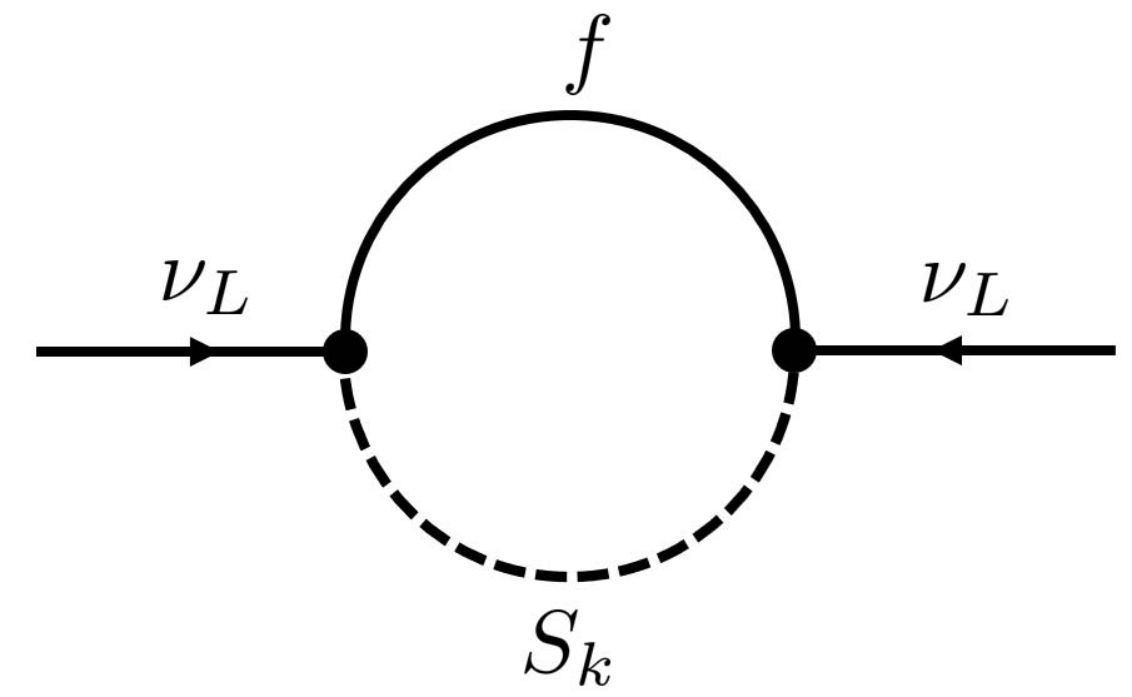
where the first term is the (tree-level) seesaw contribution, while the second accounts for the scotogenic radiative corrections (left and right diagrams in fig. 1, respectively), where

Here, $m_{\eta_{R}}$ and $m_{\eta_{I}}$ are the masses of the real and imaginary parts of $\eta=\eta_{\rm R}+i\eta_{\rm I}$. Clearly this model can accommodate neutrino data, predicting the lightest neutrino to be massless. Notice however that, beyond this, there are no other predictions that can restrict, say, the oscillation parameters.

An interesting scenario may be realized by requiring that (1) is invariant under CP and, thus, all couplings and masses are real. Clearly, in this case there is no leptonic CP violation (LCPV). However, introducing a complex scalar singlet $\sigma$ which acquires a complex VEV $\left\langle\sigma\right\rangle=ue^{i\theta}$ will potentially induce LCPV via couplings of $\nu_{R}$ and $f$ with $\sigma$ and $\sigma^{\ast}$ [35, 36]. In the most general case, these couplings are

Taking now into account that $\langle\sigma\rangle=ue^{i\theta}$, and expressing $M_{R,f}$ in (1) as $M_{R,f}=|M_{R,f}|e^{i\theta_{R,f}}$, one has for the effective neutrino mass matrix (2):

with

which shows that, in general, $\theta_{f}-\theta_{R}\neq 0$ and CP violation will be successfully communicated to the neutrino sector provided that $\theta\neq k\pi$ ($k=1,2,...$) and $y_{R,f}\neq\tilde{y}_{R,f}$.¹¹ 1 Notice that, even if $\theta\neq k\pi$, one can have $\theta_{f}-\theta_{R}=0$ if, for instance, both $\nu_{R}$ and $f$ acquire their mass just from coupling with $\sigma$ or $\sigma^{\ast}$. The diagrammatic realization of what has just been described is depicted in fig. 2 where it can be clearly seen that CP-violation in $\mathbf{M}_{\nu}$ requires a relative phase among the coefficients of the dimension-6 operators $LL\Phi\Phi\sigma$ and $LL\Phi\Phi\sigma^{\ast}$ stemming from the tree-level and scotogenic diagrams. Notice that, in this case, there are still nine parameters in (1), namely six real couplings in $\mathbf{Y}_{\nu}$ and $\mathbf{Y}_{f}$, the two masses $M_{R,f}$ and the relative phase $\theta_{R}-\theta_{f}$, which is higher than the seven effective neutrino parameters.

The minimal scoto-seesaw model, with just one copy of $\nu_{R}$ and $f$ fermions, does not offer a promising setup to implement neutrino predictions. In fact, any attempt to use an Abelian symmetry as a flavour symmetry to reduce the number of free parameters is likely to fail, as it will lead to incompatibility with neutrino oscillation data due to an unwanted extra massless neutrino or a vanishing leptonic mixing angle. Here, we extend the minimal scoto-seesaw model so as to implement a horizontal (flavour) symmetry which breaks to the dark $\mathcal{Z}_{2}$ subgroup responsible for dark matter stability. We do this by adding another $\nu_{R}$ in the fermion sector. Our template is then the (3,2) seesaw scheme [32]. In this case we add just two heavy singlet neutral leptons $\nu_{1R}$ and $\nu_{2R}$ to the Standard Model, along with the minimal dark sector with $\eta$ and $f$.

The lepton Yukawa and mass Lagrangian is identical to (1) with $\nu_{R}$ replaced by $(\nu_{1R}\,\,\nu_{2R})^{T}$, and $M_{R}$ replaced by a $2\times 2$ symmetric matrix $\mathbf{M}_{R}$. In this case, the most constraining patterns for the Yukawa and mass matrices compatible with neutrino data are [37, 38, 39]:

with $\mathbf{Y}_{\nu}$ now promoted to a $3\times 2$ matrix. As will be seen later, the texture zeros in the matrices of (7) can be moved up-and-down, as long as the total number of texture zeros is kept constant. At this point, we seek for the simplest symmetry which leads to the above patterns and allows for CP to be broken spontaneously through the VEV of the complex scalar singlet $\sigma$, as discussed above. On the other hand, since $\sigma$ couples to $\nu_{1R}$, $\nu_{2R}$ and $f$, the complex phase $\theta$ in $\left\langle\sigma\right\rangle=ue^{i\theta}$ is communicated to the effective light neutrino mass matrix. This gives rise to CPV in the neutrino sector ²² 2 Notice that, since $\eta$ will not acquire a VEV, spontaneous CPV cannot be achieved via the Standard Model Higgs doublet VEVs.. The relevant couplings which contribute to $\mathbf{M}_{R}$ and $M_{f}$ in eq. (1) are thus

where $\mathbf{Y}_{R}$, $\widetilde{\mathbf{Y}}_{R}$ are now $2\times 2$ Yukawa matrices, while $y_{f}$ and $\widetilde{y}_{f}$ are complex numbers. In searching for an Abelian $\mathcal{Z}_{N}$ symmetry which realizes (7) we must take into account that ³³ 3 Continuous $U(1)$ symmetries will not be suitable for our purposes, since the presence of the $\sigma^{4}$ term requires $\sigma$ to have no $U(1)$ charge. As a result $M_{R}$ would receive both bare and $\sigma$-induced contributions.

• •

  The $\mathbf{Y}_{\nu}$ pattern (7) requires the charges of $\nu_{R}^{1}$ and $\nu_{R}^{2}$ to be different and the mixing between the $\nu_{R}$ and $f$ to be forbidden. So we take a symmetry with at least three distinct non-trivial charges, i.e. $\mathcal{Z}_{N}$, with $N\geq 4$.

• •

  In order to guarantee that $\mathbf{M}_{R}$ has a texture zero, one of the $\nu_{R}^{1,2}$ must have a non-trivial (even) charge under the $\mathcal{Z}_{N}$ symmetry ($N\geq 4$). In $\mathcal{Z}_{4}$, that does not happen since the only two even charges are 0 and 2, which multiplied by two gives zero or $N$ and hence will not lead to texture zeros.

• •

  The dark sector particles (in the scotogenic loop) should not mix with the remaining particles. This can be achieved if their $\mathcal{Z}_{N}$ charges are distinct from those of the other particles. In addition, to ensure the stability of the lightest dark particle we require that a) the scalar $\sigma$ carries a non-trivial $\mathcal{Z}_{N}$ charge, so that its VEV breaks $\mathcal{Z}_{N}\to\mathcal{Z}_{2}$, and b) under the residual $\mathcal{Z}_{2}$ subgroup all dark sector particles have “odd” charge, while other particles are “even”. All scalar fields with odd charges must not acquire VEV, so as to preserve the residual dark symmetry. Given these conditions one can see that “odd” $\mathcal{Z}_{N}$ groups like $\mathcal{Z}_{5}$ will not work. This is due to the fact that for odd $\mathcal{Z}_{N}$ groups if we assign an odd charge to a given dark field then its Hermitian conjugate will always have an even charge under the odd $\mathcal{Z}_{N}$, hence it can mix with other particles with even $\mathcal{Z}_{N}$ charge. In conclusion, for odd $\mathcal{Z}_{N}$ groups, one cannot ensure dark matter stability [11, 13].

• •

  The symmetry must allow for quartic $\sigma^{4}$ terms in the scalar potential, though it may be softly broken by $\sigma^{2}$ terms. The $\mathcal{Z}_{5}$, $\mathcal{Z}_{6}$ and $\mathcal{Z}_{7}$ groups do not work since invariance of the $\sigma^{4}$, needed to implement SCPV, cannot be ensured.

Putting things together we conclude that the minimal required symmetry to reproduce the textures in (7) is $\mathcal{Z}_{8}$. In table 1, we show the matter content and possible charge assignments for our models. As shown in that table, there are in fact three possible assignments which we label as $\mathcal{Z}^{e-\mu}_{8}$, $\mathcal{Z}^{\mu-\tau}_{8}$ and $\mathcal{Z}^{e-\tau}_{8}$. Hence one can consider three distinct models. Notice that just with the scalars $\Phi$, $\eta$ and $\sigma$, only the tree-level seesaw contributes to the effective neutrino mass matrix. This follows from the fact that the scotogenic loop of fig. 1 requires a $\mathcal{Z}_{8}$ explicit breaking term $(\phi^{\dagger}\eta)^{2}$. Moreover, as discussed below, just with the tree-level seesaw contribution, the complex phase of the $\sigma$ VEV does not lead to leptonic CP violation. Hence, we add a second dark sector complex singlet $\chi$ transforming under $\mathcal{Z}_{8}$ as shown in table 1. The scalar potential of the model is then

where all parameters are real so as to ensure CP invariance at the Lagrangian level. Notice that the three last terms allow for the one-loop scotogenic diagrams in fig. 3. These contribute to neutrino mass generation at lowest dimension of the neutrino mass operators.

We now turn to the issue of SCPV. As shown in the Appendix, the minimisation of the scalar potential can lead to a VEV configuration with $\left\langle\eta^{0}\right\rangle=0$, $\left\langle\chi\right\rangle=0$, $\left\langle\phi^{0}\right\rangle=v$ and $\left\langle\sigma\right\rangle=ue^{i\theta}$, provided:

Note that the presence of the scalar singlet $\chi$ plays a key role in our model to prevent the explicit breaking of $\mathcal{Z}_{8}$ in the scotogenic loop.

An effective neutrino mass matrix analogous to the one in eq. (2) can now be written as,

where $\mathbf{Y}_{\nu}$ is the Dirac neutrino Yukawa coupling matrix and $\mathbf{Y}_{f}$ is the matrix of Yukawa-type couplings of the leptons to the dark fields $f$ and $\eta$. $\mathbf{M}_{R}$ is the right-handed neutrino mass matrix and $M_{f}$ is the $f$ mass. The first term in eq. (11) is the seesaw contribution, while the radiative corrections are given by the second term. The latter are characterized by the loop function $\mathcal{F}(M_{f},m_{S_{i}})$, depending on the mass eigenstates resulting from the mixing of the neutral components of $\eta$ and $\chi$ (see Appendix). While in general, $\mathbf{Y}_{\nu}$, $\mathbf{Y}_{f}$, and $\mathbf{M}_{R}$ are complex $3\times 2$, $3\times 1$ and $2\times 2$ matrices, we assume that CP is conserved at the Lagrangian level. In this case the only form of breaking is spontaneous, dictated by the complex VEV $\left\langle\sigma\right\rangle=ue^{i\theta}$ of the $\sigma$ field in which the phase is determined through eq. (10).

For definiteness let us focus on the model defined by the $\mathcal{Z}^{e-\tau}_{8}$ charge assignment in table 1. Taking into account eqs. (8) and (11), we find the following form for the Yukawa and mass matrices

where $M_{12}={(\mathbf{Y}_{R})}_{12}u$ and $M_{22}$ are invariant bare masses. Due to the initially imposed CP invariance, the parameters $x_{i}$, $y_{i}$, $w_{i}$ and $M_{1,2}$ are real. Notice also that the $f$ mass term is $M_{f}e^{-i\theta}$ with $M_{f}=y_{f}u$. The resulting $\mathcal{Z}_{8}$-invariant $\mathbf{Y}_{\ell}$ texture implies that one of the charged-leptons is decoupled from the remaining two in the symmetry basis. Thus, the contribution to lepton mixing coming from the charged lepton sector is non-trivial, being parametrized by a single angle $\theta_{\ell}$. Consequently, the unitary transformation which brings the $\ell_{i}$ fields to the mass-eigenstate basis is

where $\theta_{\ell}$ is the mixing angle. The permutation matrices obey $\mathbf{P}_{ij}=\mathbf{P}_{12},$ $\mathbb{1}$ or $\mathbf{P}_{23}$ depending on whether the decoupled charged lepton is the electron ($\mathcal{Z}^{\mu-\tau}_{8}$ symmetry), muon ($\mathcal{Z}^{e-\tau}_{8}$ symmetry) or tau ($\mathcal{Z}^{e-\mu}_{8}$ symmetry), respectively, i.e.

and $\mathbb{1}$ the $3\times 3$ identity matrix. The charged-lepton and effective neutrino mass matrices in the charged-lepton physical basis are then

with $\mathbf{M}_{\nu}$ and $\mathbf{U}_{\ell}$ given in eqs. (11) and (13), respectively. Taking into account eqs. (11) and (12), the effective neutrino mass matrix in the original symmetry basis is given by

where the texture zero $(\mathbf{M}_{\nu})_{22}=0$ results from the assumed $\mathcal{Z}^{e-\tau}_{8}$ symmetry. It can be shown that the contribution of the scotogenic loop is crucial to ensure the existence of CP violation since, in its absence, the vacuum phase $\theta$ can be rephased away. In fact, by computing $\mathcal{J}_{\text{CP}}=\text{Tr}[(\mathbf{M}_{\nu}\mathbf{M}_{\nu}^{\dagger})^{*},\mathbf{M}_{\ell}\mathbf{M}_{\ell}^{\dagger}]$, one concludes that $\mathcal{J}_{\text{CP}}=0$ if $y_{1}=y_{2}=0$, i.e., if the loop contribution vanishes. Notice also that, since the charged-lepton sector has an unmixed state, the vanishing-element condition in $\mathbf{M}_{\nu}$ remains after performing the $\mathbf{U}_{\ell}$ rotation of eq. (15). Namely,

with $i=1,2,3$ for $e,\,\mu$ and $\tau$, respectively.

In order to analyse the constraints imposed by (19) on the low-energy neutrino parameters, we express $\mathbf{M}_{\nu}^{\prime}$ in terms of the lepton mixing angles and neutrino masses. Namely,

where $m_{i}$ are the real and positive light neutrino masses and $\mathbf{U}$ is the lepton mixing matrix. Using the above equation one can reconstruct the effective neutrino mass matrix from the low-energy parameters.

After eliminating unphysical phases [32], $\mathbf{U}$ can be parametrized in a symmetrical way [40] as

where $\theta_{ij}$ ($i<j=1,2,3$) are the lepton mixing angles (with $s_{ij}\equiv\sin\theta_{ij}$, $c_{ij}\equiv\cos\theta_{ij}$). Here, $\delta=\phi_{13}-\phi_{12}-\phi_{23}$ is the Dirac CP-violating phase relevant for neutrino oscillations and $\phi_{12,13}$ are the two Majorana phases. For normal and inverted neutrino mass ordering (NO and IO, respectively) two neutrino masses are expressed in terms of the lightest neutrino mass $m_{\rm lightest}$ (which coincides with $m_{1}$ and $m_{3}$ for NO and IO, respectively), and the measured neutrino mass-squared differences $\Delta m^{2}_{21}=m_{2}^{2}-m_{1}^{2}$ and $\Delta m^{2}_{31}=m_{3}^{2}-m_{1}^{2}$ as

The current experimental ranges extracted from global fits of neutrino oscillation data are shown in table 2, from [22].

In figs. 5 and 6 we present the $1\sigma$, $2\sigma$ and $3\sigma$ allowed regions in the ($\theta_{23}$,$\delta$) and ($m_{\rm lightest}$,$\delta$) planes, for decoupled $e$, $\mu$ and $\tau$ schemes, with both NO (upper panels) and IO (lower panels) neutrino mass spectra. These distinct cases are labeled as NO_e,μ,τ and IO_e,μ,τ, respectively. To compute the $\chi^{2}$ we use the one-dimensional global-fit profiles also from [22] for $s_{12}^{2}$, $s_{13}^{2}$, $\Delta m_{21}^{2}$ and $\Delta m_{31}^{2}$. Due to the correlations observed between $\theta_{23}$ and $\delta$, we use instead for these two parameters a two-dimensional $\chi^{2}$ distribution, also from Ref. [22]. Notice that we do not include in the fit the constraints on $m_{\rm lightest}$ coming from $\beta$-decay experiments or cosmology. Instead, in fig. 6 we display our results in terms of $m_{\rm lightest}$ and indicate these bounds by vertical red dashed line and a shaded band, respectively. The vertical dashed red line corresponds to the $m_{\text{lightest}}$ KATRIN tritium beta decay upper limit $m_{\beta}<1.1$ eV (90% CL). On the other hand the band delimits the conservative and agressive upper limits from cosmology, as indicated in the caption. The right (left) delimiting black dotted limit corresponds to the Planck TT+lowE (Planck TT, TE, EE+lowE+lensing+BAO) 95% CL limit $\sum_{k}m_{k}<0.54$ eV ($0.12$ eV). Notice that the fitting procedure is always performed under the theoretical assumption expressed by relation (19) for each of the three cases to be analysed. We also include in fig. 5 the (dashed) lines delimiting the regions implied by data only, i.e. without any “prior” input from the model.

Examining these figures we conclude the following:

• •

  The IO_e case is not compatible with data since the condition $(\mathbf{M}_{\nu}^{\prime})_{11}=0$ leads to a vanishing $\rm 0\nu\beta\beta$ decay rate. The latter is well-known to be inconsistent with inverse ordering.

• •

  As seen in the leftmost upper panel in fig. 5, for the NO_e case the model-allowed regions in ($\theta_{23}$,$\delta$) coincide with the generic ones obtained in the global fit of experimental data. This is due to the fact that $(\mathbf{M}_{\nu}^{\prime})_{11}$ does not depend on $\theta_{23}$ and $\delta$. However, $(\mathbf{M}_{\nu}^{\prime})_{11}=0$ is only satisfied in the $(m_{\rm lightest},\delta)$ allowed regions shown in the corresponding plot of fig. 6. In particular, compatibility with data in the NO_e case requires $m_{\rm lightest}\sim[20,80]$ meV, at the $3\sigma$ level. This leads to a lower bound on $m_{\rm lightest}$. Moreover, it implies an upper bound on $m_{\rm lightest}$ which is more stringent than those which follow from current cosmology and the kinematics of tritium beta decays. These are indicated in fig. 6 by a vertical shaded band and a red dashed line, respectively.

• •

  The NO_μ (NO_τ) case selects the first (second) octant for $\theta_{23}$, as can be seen in the middle (rightmost) upper plot of fig. 5. This can also be seen in fig. 4. Consequently, while NO_τ is compatible with data at $1\sigma$, for NO_μ this happens only at $2\sigma$. The preference for a different $\theta_{23}$ octant in each of these two cases is interesting since future experiments, such as T2HK, might in principle resolve the ambiguity and, hence exclude either NO_μ or NO_τ.

• •

  For the IO_μ,τ cases the $(\theta_{2,3},\delta)$ regions coincide with those given by the current global fits, see lower panels in figs. 5, indicating that the model can accommodate neutrino oscillation data within the corresponding $(m_{\rm lightest},\delta)$ regions (lower panels in fig. 6). One sees that for IO_μ the $m_{\rm lightest}$ range is $[5,100]$ meV at $1\sigma$, with the best-fit value at $\sim 10$ meV. As for IO_τ, there is a $1\sigma$ lower bound of $16$ meV, which lies in the left border of the cosmological bound band.

Given the results just obtained for the oscillations parameters and the lightest neutrino mass, we now present the allowed regions for the effective mass parameter $m_{\beta\beta}$ characterizing the amplitude for neutrinoless double beta decay. In the symmetrical parametrization of the lepton mixing matrix [32, 40] the contribution arising from the exchange of light neutrinos gives

for the NO and IO cases respectively.

In fig. 7 we show the predictions for $m_{\beta\beta}$ taking into account the global oscillation analysis in Ref. [22]. The results are given in terms of $m_{\rm lightest}$ and correspond to those of figs. 5 and 6. The upper panels correspond to the NO case, while the lower ones are for the IO. The present upper bounds coming from $\rm 0\nu\beta\beta$ searches at KamLAND-Zen 400 [41], GERDA [42], CUORE [43] and EXO-200 [44] are also indicated. Note that the case NO_e predicts $m_{\beta\beta}=0$ and is not shown. From the results presented in that figure one sees that there is a lower bound on the $\rm 0\nu\beta\beta$ amplitude that holds even if the neutrino mass spectrum is normal ordered. Although this feature occurs in many family symmetry schemes where the cancellation is prevented by the structure of the leptonic weak interaction vertex [45, 46, 47], it is remarkable that it holds here, with just such a simple Abelian $\mathcal{Z}_{8}$ symmetry. In fact, one sees that the current KamLAND bound for $m_{\beta\beta}$ nearly excludes the NO cases. Future data from upcoming projects like AMORE II [48], CUPID [49], LEGEND [50], SNO+ I [51], KamLAND2-Zen [41], nEXO [52] or PandaX-III [53] should probe the entire allowed regions. For the inverted ordering cases one sees that the allowed regions are also meaningfully probed by the current $m_{\beta\beta}$ upper bound. However, they will be fully probed by the expected sensitivities from upcoming experiments.

We have proposed a simple scoto-seesaw model based on a $\mathcal{Z}_{8}$ flavour symmetry which is broken to a dark $\mathcal{Z}_{2}$ by a scalar singlet $\sigma$ VEV. This complex vacuum expectation value is the unique source of leptonic CP violation, that takes place in a spontaneous manner. Such CPV is communicated to the leptonic sector via couplings of $\sigma$ with the $\nu_{R}$ and the dark fermion $f$. We have shown that the $\mathcal{Z}_{8}$ symmetry leads to constraints on the low-energy parameters. Except for the case in which $m_{\beta\beta}=0$, the predicted ranges on the lightest-neutrino mass for a normal ordered neutrino spectrum will be fully tested by future neutrinoless double beta decay experiments and by improved neutrino mass sensitivities from cosmological probes. In the inverted ordering case, a better determination of the Dirac CPV phase $\delta$ is required to test the model under scrutiny. More than proposing yet another model for neutrino masses and dark matter, our work intends to establish a template for a dynamical origin of leptonic CP violation. This is achieved by combining the neutrino mass generation mechanism and the solution of the dark matter problem. CP violation is driven by the same scalar singlet VEV providing mass to the heavy light-neutrino mass mediator fermions.

*

References

- [1] A. B. McDonald, “Nobel Lecture: The Sudbury Neutrino Observatory: Observation of flavor change for solar neutrinos,” Rev.Mod.Phys. 88 (2016) 030502.
- [2] T. Kajita, “Nobel Lecture: Discovery of atmospheric neutrino oscillations,” Rev.Mod.Phys. 88 (2016) 030501.
- [3] H. Ishimori, T. Kobayashi, H. Ohki, Y. Shimizu, H. Okada, and M. Tanimoto, “Non-Abelian Discrete Symmetries in Particle Physics,” Prog.Theor.Phys.Suppl. 183 (2010) 1–163, arXiv:1003.3552 [hep-th].
- [4] G. Bertone, D. Hooper, and J. Silk, “Particle dark matter: Evidence, candidates and constraints,” Phys.Rept. 405 (2005) 279–390.
- [5] E. Ma, “Verifiable radiative seesaw mechanism of neutrino mass and dark matter,” Phys.Rev. D73 (2006) 077301.
- [6] E. Ma and D. Suematsu, “Fermion Triplet Dark Matter and Radiative Neutrino Mass,” Mod.Phys.Lett. A24 (2009) 583–589, arXiv:0809.0942 [hep-ph].
- [7] M. Hirsch et al., “WIMP dark matter as radiative neutrino mass messenger,” JHEP 1310 (2013) 149, arXiv:1307.8134 [hep-ph].
- [8] A. Merle et al., “Consistency of WIMP Dark Matter as radiative neutrino mass messenger,” JHEP 1607 (2016) 013, arXiv:1603.05685 [hep-ph].
- [9] M. A. Díaz et al., “Heavy Higgs Boson Production at Colliders in the Singlet-Triplet Scotogenic Dark Matter Model,” JHEP 1708 (2017) 017, arXiv:1612.06569 [hep-ph].
- [10] S. Choubey, S. Khan, M. Mitra, and S. Mondal, “Singlet-Triplet Fermionic Dark Matter and LHC Phenomenology,” Eur.Phys.J. C78 (2018) 302, arXiv:1711.08888 [hep-ph].
- [11] C. Bonilla, S. Centelles-Chuliá, R. Cepedello, E. Peinado, and R. Srivastava, “Dark matter stability and Dirac neutrinos using only Standard Model symmetries,” Phys. Rev. D 101 no. 3, (2020) 033011, arXiv:1812.01599 [hep-ph].
- [12] S. Centelles Chuliá, R. Cepedello, E. Peinado, and R. Srivastava, “Scotogenic dark symmetry as a residual subgroup of Standard Model symmetries,” Chin. Phys. C 44 no. 8, (2020) 083110, arXiv:1901.06402 [hep-ph].
- [13] C. Bonilla, E. Peinado, and R. Srivastava, “The role of residual symmetries in dark matter stability and the neutrino nature,” LHEP 2 no. 1, (2019) 124, arXiv:1903.01477 [hep-ph].
- [14] S. Centelles Chuliá, R. Cepedello, E. Peinado, and R. Srivastava, “Systematic classification of two loop = 4 Dirac neutrino mass models and the Diracness-dark matter stability connection,” JHEP 10 (2019) 093, arXiv:1907.08630 [hep-ph].
- [15] D. Restrepo and A. Rivera, “Phenomenological consistency of the singlet-triplet scotogenic model,” JHEP 2004 (2020) 134, arXiv:1907.11938 [hep-ph].
- [16] I. M. Ávila, V. De Romeri, L. Duarte, and J. W. Valle, “Minimalistic scotogenic scalar dark matter,” arXiv:1910.08422 [hep-ph].
- [17] S. K. Kang, O. Popov, R. Srivastava, J. W. Valle, and C. A. Vaquera-Araujo, “Scotogenic dark matter stability from gauged matter parity,” Phys.Lett. B798 (2019) 135013, arXiv:1902.05966 [hep-ph].
- [18] J. Leite, O. Popov, R. Srivastava, and J. W. Valle, “A theory for scotogenic dark matter stabilised by residual gauge symmetry,” arXiv:1909.06386 [hep-ph].
- [19] A. Cárcamo Hernández, J. W. Valle, and C. A. Vaquera-Araujo, “Simple theory for scotogenic dark matter with residual matter-parity,” arXiv:2006.06009 [hep-ph].
- [20] J. Leite, A. Morales, J. W. Valle, and C. A. Vaquera-Araujo, “Dark matter stability from Dirac neutrinos in scotogenic 3-3-1-1 theory,” arXiv:2005.03600 [hep-ph].
- [21] J. Leite, A. Morales, J. W. Valle, and C. A. Vaquera-Araujo, “Scotogenic dark matter and Dirac neutrinos from unbroken gauged symmetry,” arXiv:2003.02950 [hep-ph].
- [22] P. de Salas et al., “2020 Global reassessment of the neutrino oscillation picture,” arXiv:2006.11237 [hep-ph].
- [23] N. Rojas, R. Srivastava, and J. W. F. Valle, “Simplest Scoto-Seesaw Mechanism,” Phys.Lett. B789 (2019) 132–136, arXiv:1807.11447 [hep-ph].
- [24] E. Ma and G. Rajasekaran, “Softly broken A(4) symmetry for nearly degenerate neutrino masses,” Phys. Rev. D 64 (2001) 113012, arXiv:hep-ph/0106291.
- [25] K. Babu, E. Ma, and J. Valle, “Underlying A(4) symmetry for the neutrino mass matrix and the quark mixing matrix,” Phys.Lett. B552 (2003) 207–213.
- [26] G. Altarelli and F. Feruglio, “Tri-bimaximal neutrino mixing, A(4) and the modular symmetry,” Nucl.Phys. B741 (2006) 215–235.
- [27] E. Ma and R. Srivastava, “Dirac or inverse seesaw neutrino masses with gauge symmetry and flavor symmetry,” Phys. Lett. B 741 (2015) 217–222, arXiv:1411.5042 [hep-ph].
- [28] F. J. de Anda, J. W. Valle, and C. A. Vaquera-Araujo, “Flavour and CP predictions from orbifold compactification,” Phys.Lett. B801 (2020) 135195, arXiv:1910.05605 [hep-ph].
- [29] F. J. de Anda, N. Nath, J. W. Valle, and C. A. Vaquera-Araujo, “Probing the predictions of an orbifold theory of flavor,” arXiv:2004.06735 [hep-ph].
- [30] P. Chen, G.-J. Ding, J.-N. Lu, and J. W. Valle, “Predictions from warped flavordynamics based on the family group,” arXiv:2003.02734 [hep-ph].
- [31] J. Schechter and J. W. F. Valle, “Comment on the Lepton Mixing Matrix,” Phys.Rev. D21 (1980) 309.
- [32] J. Schechter and J. W. F. Valle, “Neutrino Masses in SU(2) x U(1) Theories,” Phys.Rev. D22 (1980) 2227.
- [33] M. Reig, D. Restrepo, J. W. F. Valle, and O. Zapata, “Bound-state dark matter with Majorana neutrinos,” Phys. Lett. B790 (2019) 303–307, arXiv:1806.09977 [hep-ph].
- [34] S. Mandal, R. Srivastava, and J. W. Valle, “Consistency of the dynamical high-scale type-I seesaw mechanism,” Phys. Rev. D 101 no. 11, (2020) 115030, arXiv:1903.03631 [hep-ph].
- [35] G. C. Branco, L. Lavoura, and J. P. Silva, “CP Violation,” Int.Ser.Monogr.Phys. 103 (1999) 1–536.
- [36] G. Branco, R. Felipe, and F. Joaquim, “Leptonic CP Violation,” Rev. Mod. Phys. 84 (2012) 515–565, arXiv:1111.5332 [hep-ph].
- [37] D. Barreiros, R. Felipe, and F. Joaquim, “Minimal type-I seesaw model with maximally restricted texture zeros,” Phys. Rev. D 97 no. 11, (2018) 115016, arXiv:1802.04563 [hep-ph].
- [38] D. Barreiros, R. Felipe, and F. Joaquim, “Combining texture zeros with a remnant CP symmetry in the minimal type-I seesaw,” JHEP 01 (2019) 223, arXiv:1810.05454 [hep-ph].
- [39] D. Barreiros, F. Joaquim, and T. Yanagida, “New approach to neutrino masses and leptogenesis with Occam’s razor,” Phys. Rev. D 102 no. 5, (2020) 055021, arXiv:2003.06332 [hep-ph].
- [40] W. Rodejohann and J. W. F. Valle, “Symmetrical Parametrizations of the Lepton Mixing Matrix,” Phys. Rev. D 84 (2011) 073011, arXiv:1108.3484 [hep-ph].
- [41] KamLAND-Zen Collaboration, A. Gando et al., “Search for Majorana Neutrinos near the Inverted Mass Hierarchy Region with KamLAND-Zen,” Phys. Rev. Lett. 117 no. 8, (2016) 082503, arXiv:1605.02889 [hep-ex]. [Addendum: Phys.Rev.Lett. 117, 109903 (2016)].
- [42] GERDA Collaboration, M. Agostini et al., “Final Results of GERDA on the Search for Neutrinoless Double- Decay,” arXiv:2009.06079 [nucl-ex].
- [43] CUORE Collaboration, D. Adams et al., “Improved Limit on Neutrinoless Double-Beta Decay in 130Te with CUORE,” Phys. Rev. Lett. 124 no. 12, (2020) 122501, arXiv:1912.10966 [nucl-ex].
- [44] EXO-200 Collaboration, G. Anton et al., “Search for Neutrinoless Double- Decay with the Complete EXO-200 Dataset,” Phys. Rev. Lett. 123 no. 16, (2019) 161802, arXiv:1906.02723 [hep-ex].
- [45] L. Dorame et al., “Constraining Neutrinoless Double Beta Decay,” Nucl.Phys. B861 (2012) 259–270, arXiv:1111.5614 [hep-ph].
- [46] L. Dorame et al., “A new neutrino mass sum rule from inverse seesaw,” Phys.Rev. D86 (2012) 056001, arXiv:1203.0155 [hep-ph].
- [47] S. King et al., “Quark-Lepton Mass Relation in a Realistic Extension of the Standard Model,” Phys.Lett. B724 (2013) 68–72, arXiv:1301.7065 [hep-ph].
- [48] AMoRE Collaboration, M. H. Lee, “AMoRE: A search for neutrinoless double-beta decay of 100Mo using low-temperature molybdenum-containing crystal detectors,” JINST 15 no. 08, (2020) C08010, arXiv:2005.05567 [physics.ins-det].
- [49] CUPID Collaboration, G. Wang et al., “CUPID: CUORE (Cryogenic Underground Observatory for Rare Events) Upgrade with Particle IDentification,” arXiv:1504.03599 [physics.ins-det].
- [50] LEGEND Collaboration, N. Abgrall et al., “The Large Enriched Germanium Experiment for Neutrinoless Double Beta Decay (LEGEND),” vol. 1894, p. 020027. 2017. arXiv:1709.01980 [physics.ins-det].
- [51] SNO+ Collaboration, S. Andringa et al., “Current Status and Future Prospects of the SNO+ Experiment,” Adv. High Energy Phys. 2016 (2016) 6194250, arXiv:1508.05759 [physics.ins-det].
- [52] nEXO Collaboration, J. Albert et al., “Sensitivity and Discovery Potential of nEXO to Neutrinoless Double Beta Decay,” Phys. Rev. C 97 no. 6, (2018) 065503, arXiv:1710.05075 [nucl-ex].
- [53] X. Chen et al., “PandaX-III: Searching for neutrinoless double beta decay with high pressure136Xe gas time projection chambers,” Sci. China Phys. Mech. Astron. 60 no. 6, (2017) 061011, arXiv:1610.08883 [physics.ins-det].
- [54] G. Lazarides, M. Reig, Q. Shafi, R. Srivastava, and J. W. Valle, “Spontaneous Breaking of Lepton Number and the Cosmological Domain Wall Problem,” Phys. Rev. Lett. 122 no. 15, (2019) 151301, arXiv:1806.11198 [hep-ph].