Holographic Entanglement Entropy of the Coulomb Branch
Abstract
We compute entanglement entropy (EE) of a spherical region in -dimensional supersymmetric Yang-Mills theory in states described holographically by probe D3-branes in . We do so by generalising methods for computing EE from a probe brane action without having to determine the probe’s back-reaction. On the Coulomb branch with broken to , we find the EE monotonically decreases as the sphere’s radius increases, consistent with the -theorem. The EE of a symmetric-representation Wilson line screened in also monotonically decreases, although no known physical principle requires this. A spherical soliton separating inside from outside had been proposed to model an extremal black hole. However, we find the EE of a sphere at the soliton’s radius does not scale with the surface area. For both the screened Wilson line and soliton, the EE at large radius is described by a position-dependent W-boson mass as a short-distance cutoff. Our holographic results for EE and one-point functions of the Lagrangian and stress-energy tensor show that at large distance the soliton looks like a Wilson line in a direct product of fundamental representations.
Keywords
AdS/CFT Correspondence, Gauge/Gravity Correspondence, Conformal Field Theory, Supersymmetric Gauge Theory1 Introduction
Quantum entanglement is of fundamental importance, being a manifestation of purely quantum correlations. For a bipartite system in a pure state, the amount of entanglement between the two complementary subspaces may be quantified by entanglement entropy (EE), defined as the von Neumann entropy of the reduced density matrix of one of the subspaces Bombelli:1986rw; Bennett:1995tk. EE plays a prominent role in disparate areas of physics. For instance, in quantum field theory (QFT) the EE of a spatial subregion has ultraviolet (UV) divergences due to correlations across the subregion’s boundary. The leading divergence is proportional to the subregions’ surface area Srednicki:1993im. This area law received much attention in attempts to understand the Bekenstein-Hawking entropy of black holes. EE also plays a prominent role in condensed matter physics Amico:2007ag; Eisert:2008ur; specialissue, for example as a probe of quantum phase transitions Vidal:2002rm.
Besides the leading area law term, EE contains subleading divergences and finite contributions that can provide important information Callan:1994py; Holzhey:1994we; Solodukhin:1994yz; Solodukhin:1994st; Fursaev:1995ef. For example, in -dimensional critical systems the EE of an interval has a logarithmic violation of the area law driven by the central charge Holzhey:1994we; Calabrese:2004eu; Calabrese:2009qy. This feature makes the EE a good quantity from which to infer the universality class of spin chains from numerical computations Peschel:2004qbn; Its_2005; Sugino_2018.
More generally, a logarithmic divergence arises in the EE of any even-dimensional conformal field theory (CFT). Its coefficient, which is universal and regularisation independent, turns out to be a linear combination of the CFT’s central charges. This opened a new perspective on monotonicity theorems, such as the well-known -theorem in dimensions Zamolodchikov:1986gt. Indeed, ref. Casini:2004bw proved an entropic version of the -theorem: in any Lorentz invariant QFT describing a renormalisation group (RG) flow from a UV CFT to an infrared (IR) CFT, a certain -function, defined from a spatial interval’s EE, decreases monotonically with the interval’s length, and agrees with the central charge in the limits of zero length (the UV) and infinite length (the IR). In higher dimensions EE has been used to prove similar monotonicity theorems, such as the -dimensional -theorem Jafferis:2011zi; Casini:2012ei and the -dimensional -theorem Cardy:1988cwa; Osborn:1989td; Jack:1990eb; Komargodski:2011vj; Solodukhin:2013yha; Casini:2017vbe.
While string theory has provided methods to compute black hole entropy Strominger:1996sh, the anti-de Sitter/conformal field theory (AdS/CFT) correspondence Maldacena; Witten:1998qj; Gubser:1998bc; Aharony:1999ti, otherwise known as holography, renewed interest in EE in the high-energy physics community. For a gauge theory at large and strong coupling with a holographic dual, Ryu and Takayanagi (RT) proposed that the EE of a spatial region is proportional to the area of the minimal surface extending in the holographic direction and anchored to the entangling surface at the asymptotic boundary Ryu:2006bv; Ryu:2006ef. Originally a conjecture, this prescription was later proved by Lewkowycz and Maldacena Lewkowycz:2013nqa. The RT formula and its covariant generalisation Hubeny:2007xt; Dong:2016hjy have turned out to be useful for many reasons, including two in particular.
First, holographic EE (HEE) provides a powerful tool to quantify entanglement in strongly-coupled QFTs. In general EE is difficult to compute directly in QFT, even for free theories.11 1 An exception is -dimensional CFT, where the Virasoro symmetry provides a systematic approach to computing EE Holzhey:1994we; Calabrese:2009qy. On the other hand, HEE is relatively straightforward to calculate. Second, the RT formula suggests a deep connection between entanglement and gravity. For example, refs. Swingle:2009bg; VanRaamsdonk:2009ar; VanRaamsdonk:2010pw; Maldacena:2013xja argued that the geometry of an asymptotically AdS space-time should be related to the entanglement structure of the dual QFT’s quantum state.
In this paper we use HEE to study RG flows described holographically by probe branes in AdS space-time. In the holographic framework, branes in the gravity theory can describe fields, states, and objects ranging from fields in the fundamental representation of the gauge group (i.e. flavour fields) Karch:2002sh, to baryons Witten:1998xy, to Wilson lines Maldacena:1998im; Rey:1998bq; Drukker:2005kx; Hartnoll:2006hr; Yamaguchi:2006tq; Hartnoll:2006is; Gomis:2006im, and more. Broadly speaking, a brane that reaches the AdS boundary is dual to fields added to the QFT, while a brane that does not reach the AdS boundary describes a state of the QFT.
We employ a common simplification, namely the probe limit, in which the brane’s back-reaction on the metric and other bulk fields is neglected. In the dual field theory, the probe limit corresponds to a probe sector with a number of degrees of freedom parametrically smaller in than the adjoint-representation fields’ order degrees of freedom.
How can we calculate HEE from a probe brane? More precisely, how can we holographically compute the leading contribution in to the EE from the probe sector? Given that the RT approach depends only on the metric, the obvious answer is to compute the brane’s linearised back-reaction on the metric, and from that, the resulting change in the minimal surface’s area. Although streamlined methods for doing this have been developed in certain cases Chang:2013mca; Jones:2015twa, in general this remains a difficult problem, especially for branes that break symmetries and hence may make the back-reaction complicated.
We will instead use Karch and Uhlemann’s method for computing the leading order contribution of a probe brane to HEE directly from a probe brane’s action, without computing back-reaction Karch:2014ufa. Their method generalises Lewkowycz and Maldacena’s method for proving the RT formula to probe branes (see ref. Jensen:2013lxa for precursor work in conformal cases). Refs. Vaganov:2015vpq; Kumar:2017vjv and Rodgers:2018mvq used the Karch-Uhlemann method to obtain the HEE of non-conformal D-brane and M-brane solutions, respectively.
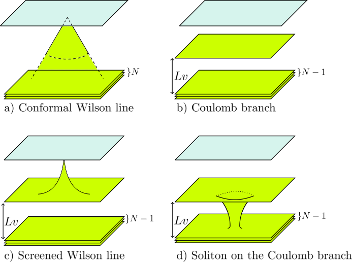
In this paper, we use the Karch-Uhlemann method to compute the contribution to HEE from various probe D3-branes in the background of type IIB supergravity. The holographically dual CFT is -dimensional supersymmetric Yang-Mills (SYM) theory with gauge group , with large and large ’t Hooft coupling, Maldacena.
This theory can be realised as the worldvolume theory of a stack of D3-branes in . The theory has a Coulomb branch of supersymmetric vacua in which the adjoint scalar superpartners of the gluons acquire non-zero vacuum expectation values (VEVs) and Higgs to a subgroup. This corresponds to separating the D3-branes from each other in transverse directions. Separations between D3-branes set the lengths of strings stretched between them, and hence the masses of the W-bosons and their superpartners.
We will focus on the situation with precisely one D3-brane separated from the stack, thus Higgsing to . In the holographic limits and we replace the stack of D3-branes with their near-horizon geometry, , and treat the single D3-brane as a probe describing an RG flow from SYM to SYM. We will also consider D3-branes that describe supersymmetric Wilson lines and spherical solitons in this vacuum.
Cartoons of the relevant D3-brane solutions are shown in figure 1, with the boundary at the top and the Poincaré horizon at the bottom. In the figure we depict the D3-branes generating , but of course these D3-branes are not actually present in , having “dissolved” into five-form flux. We show them simply for intuition.
Figure 1a depicts the D3-brane holographically dual to a straight Wilson line in the -th rank symmetric representation of , where the D3-brane carries units of string charge Drukker:2005kx; Gomis:2006sb; Hartnoll:2006is; Gomis:2006im. We show this solution at the origin of the Coulomb branch, where all D3-branes generating remain coincident. This solution is 1/2-BPS and preserves defect conformal symmetry, so we call it the (conformal) Wilson line D3-brane.
Figure 1b depicts the probe D3-brane dual to a point on the Coulomb branch where Klebanov:1999tb. This D3-brane is parallel to the other D3-branes, but is separated from them by a distance in the holographic direction, where is the radius and sets the VEV of a single adjoint scalar field. If we descend into from the boundary, then, when we cross this D3-brane, the five-form flux drops from to . Recalling that the holographic coordinate is dual to the RG scale, with the regions near the boundary and Poincaré horizon dual to the UV and IR, respectively, this probe D3-brane clearly describes an RG flow in which . We call this the Coulomb branch D3-brane.
Figure 1c depicts the D3-brane dual to the Wilson line on the Coulomb branch, now screened by the adjoint scalar VEV. In particular, as we descend into this D3-brane initially resembles the Wilson line D3-brane of figure 1a, including the units of string charge, but then interpolates smoothly to the Coulomb branch D3-brane of figure 1b. Crucially, this D3-brane is not present below . The dual CFT interpretation is that in this Coulomb branch vacuum the Wilson line present in the UV is absent in the IR, that is, the Wilson line has been screened by the adjoint scalar VEV Kumar:2016jxy; Kumar:2017vjv; Evans:2019pcs. This D3-brane is 1/2-BPS but not conformal. We call it the screened Wilson line D3-brane.
Figure 1d depicts the D3-brane dual to an excited state on the Coulomb branch, namely a spherically symmetric soliton Ghoroku:1999bc; Gauntlett:1999xz; deMelloKoch:1999ui; Schwarz:2014rxa, interpreted in refs. Schwarz:2014rxa; Schwarz:2014zsa as a phase bubble, or domain wall, separating inside from outside. Indeed, this D3-brane is essentially a Coulomb branch D3-brane with a cylindrical “spike” that reaches the Poincaré horizon with non-zero radius. This D3-brane carries units of string charge, dual to units of charge uniformly spread over the domain wall. This D3-brane is 1/2-BPS but not conformal: the soliton’s mass is . We call it the spherical soliton D3-brane.
In this paper we calculate the contribution of each probe D3-brane mentioned above to the EE of a spherical region of radius , centred on the Wilson line or spherical soliton, using the Karch-Uhlemann method. More precisely, we calculate the change in EE from the case with no probe D3-brane. This difference has no UV divergences.
For all cases except the conformal Wilson line, our results are novel, and revealing. Moreover, they provide a crucial lesson about the Karch-Uhlemann method: for non-conformal probe branes, this method requires a careful accounting for a boundary contribution on the brane worldvolume. Although this boundary term vanishes for the conformal Wilson line, it is non-zero for all our non-conformal probe branes. This boundary term has been neglected in all previous applications of the Karch-Uhlemann method Karch:2014ufa; Vaganov:2015vpq; Kumar:2017vjv; Rodgers:2018mvq.
The contribution to EE from the conformal, symmetric-representation Wilson line, , was computed using conformal symmetry and supersymmetric localisation in ref. Lewkowycz:2013laa, and using the Karch-Uhlemann method in ref. Kumar:2017vjv. We reproduce those results.
For the contribution to EE from the Coulomb branch D3-brane, , we find a new, analytical (i.e. non-numerical) result. As a non-trivial check, we reproduce our using the RT formula in the fully back-reacted solution for the Coulomb branch. We further show that our obeys the entropic -theorem Osborn:1989td; Jack:1990eb; Komargodski:2011vj; Solodukhin:2013yha; Casini:2017vbe and also the entropic “area law,” which states that the coefficient of the area law term must decrease along the RG flow Casini:2016udt; Casini:2017vbe.
We compute the contribution to EE from the screened Wilson line D3-brane, , numerically. When we find , as expected, since these two cases coincide in the UV. As increases, we find that decreases monotonically. We know of no physical principle that requires such behaviour. Indeed, this case involves an RG flow of the bulk QFT, triggered by the scalar VEV , which in turn triggers an RG flow on the Wilson line, whose degrees of freedom couple to the scalar such that the non-zero VEV acts as a mass term Maldacena:1998im; Gomis:2006sb. No monotonicity theorem is known for such a situation.
We compute the contribution to EE from the spherical soliton D3-brane, , numerically. the result is not monotonic in . When we find , as expected. As we increase we find a maximum near the domain wall, after which decreases.
Curiously, the spherical soliton’s mass and charge are both proportional to its radius. In refs. Schwarz:2014rxa; Schwarz:2014zsa Schwarz observed that an asymptotically flat extremal Reissner-Nordström black hole with sufficiently large charge shares this property, raising the question of whether the soliton reproduces any other features of extremal Reissner-Nordström. Indeed, in ref. Kumar:2020hif, some of us showed that the spherical soliton supports a spectrum of quasi-normal modes with both qualitative and quantitative similarities to those of an extremal black hole. In this paper we address one of Schwarz’s key questions, namely whether at large charge the EE of a sphere coincident with the soliton scales with surface area (after suitable regularisation), similar to a black hole’s Bekenstein-Hawking entropy. We find numerically that this EE scales not with surface area, but with a power of the soliton’s radius
In the IR limit we expect both and to approach , since in that limit all the dual D3-branes look like the Coulomb branch D3-brane. In the large- asymptotics of and we indeed find , however we also find other contributions, including a term that grows as , as well as -independent constants. Remarkably, we found a simple and intuitive way to reproduce these terms, as follows.
In figures 1b, c and d, a W-boson is dual to a string stretched between the probe D3-brane and the Poincaré horizon. In particular, the W-boson mass is the length of such a string times its tension. In SYM, the W-boson mass acts as a UV cutoff. Indeed, our result for resembles that of a CFT with this UV cutoff. In figures 1c and d the W-boson clearly acquires a position-dependent mass, hence this UV cutoff becomes position dependent. Remarkably, for and in the limit, we find that taking and replacing the constant cutoff with the position-dependent cutoff reproduces our numerical results for and up to and including order . In particular, in this reproduces the term and an -independent term linear in . In a large-, large- limit we show that this contribution arises from the part of the probe D3-brane near the Poincaré horizon, which behaves as a cylindrical shell of strings. Specifically, this contribution is precisely that of a Wilson line in the direct product of fundamental representations.
We also compute the probe sector’s contribution to the VEV of the Lagrangian, via the D3-branes’ linearised back-reaction on the dilaton. We obtain new, analytical results in various limits. For example, for the screened Wilson line, when our result resembles that of a point charge in Maxwell theory. What begins in the UV as a Wilson line of appears in the IR as a point charge of the and a singlet of . In other words, it is screened, as expected. For the spherical soliton we find a maximum near the soliton’s radius. In the large- and large- limits we compute the probe sector’s contribution to the VEVs of the Lagrangian and stress-energy tensor analytically, and find results consistent with . In particular, in each VEV, when we find a term linear in , with the form expected of a Wilson line in the direct product of fundamental representations.
All of our results for the EE of non-conformal branes rely crucially on the boundary term in the Karch-Uhlemann method, as we discuss in detail in each case. More generally, our results pave the way for pursuing many fundamental questions and applications of HEE directly in the probe limit, without computing backreaction.
This paper is organized as follows. In section 2 we review EE, the RT formula, and the Karch-Uhlemann method, and illustrate the method in a simple example, a fundamental representation Wilson line. In section 3 we review the probe D3-branes described above, and in section 4 we compute their contributions to HEE. In section 5 we compute the Lagrangian VEVs, and for the soliton, also the stress-energy tensor. Section 6 is a summary and discussion of future research. We collect many technical details in four appendices.
2 Holographic Entanglement Entropy
In this section we review the calculation of EE in holography. In section 2.1 we review the definition of EE and its computation in holography as proposed by Ryu and Takayanagi (RT) Ryu:2006bv; Ryu:2006ef. Our focus will be on AdS space-times containing one or more probe branes. A convenient method for calculating the leading order contribution of probe branes to EE was given by Karch and Uhlemann in ref. Karch:2014ufa. In section 2.2 we review their method, and highlight the presence of a contribution they neglected. This contribution, which takes the form of a boundary term on the probe brane, is in fact non-zero in all our non-conformal examples. Indeed, it can provide a crucial contribution to the EE as we will see in section 4.
2.1 Review: entanglement entropy and holography
Given a generic quantum state described by a density matrix and a bipartition of the Hilbert space into a subspace and its complement , the reduced density matrix on is defined as . The EE of is defined as the von Neumann entropy of ,
| (2.1) |
If the total state is pure, which will be the case in all that follows, then and the EE is a good measure of the amount of quantum entanglement between and .
In QFT, a natural way to partition the Hilbert space is to do so geometrically, taking to be a set of states in a subregion of a Cauchy hypersurface. The EE may then be computed through the replica trick Callan:1994py, an approach which has been particularly successful for two-dimensional CFTs Holzhey:1994we; Calabrese:2004eu; Calabrese:2009qy; Calabrese:2009ez; Calabrese:2010he. The first step of the replica trick is to construct the quantity with , which is equal to the partition function of copies of the original theory glued together along . This is equivalent to the partition function of the original theory on a manifold with conical deficit at the entangling surface between and , namely . Defining the -th Rényi entropy as
| (2.2) |
the EE is given by the limit
| (2.3) |
Defining a generating functional , eq. (2.3) may be rewritten as
| (2.4) |
This form of the EE will be useful in the following.
For a QFT with a holographic dual, the EE of a time-independent state can be computed through the RT formula Ryu:2006bv; Ryu:2006ef
| (2.5) |
where is the minimal surface in the bulk space-time homologous to the region at the asymptotic boundary, is the area of , and is Newton’s constant of the bulk gravity theory. This result was extended to time-dependent cases in refs. Hubeny:2007xt; Dong:2016hjy.
The RT formula was proved by Lewkowycz and Maldacena in ref. Lewkowycz:2013nqa by defining a generalised gravitational entropy, in an extension of the usual Gibbons-Hawking thermodynamic interpretation of Euclidean gravity solutions Gibbons:1976ue to cases with no symmetry.22 2 See also ref. Casini:2011kv for an earlier proof of the RT formula for the special case of a spherical entangling region in a CFT. Consider a semiclassical gravitational theory on a Euclidean manifold with a boundary. We assume that the boundary has a direction which is topologically a circle, parametrised by a coordinate with , but it need not have a isometry. The boundary conditions are assumed to respect ’s periodicity. In the context of EE, winds around the boundary of the subregion . Let be the on-shell action of the gravity theory with the period extended to , with , while maintaining boundary conditions invariant under . The generalised gravitational entropy is then defined as
| (2.6) |
For a theory on a static asymptotically AdS space-time, the on-shell action is equal to the dual QFT’s generating functional . The right-hand side of eq. (2.6) is then identical to the right-hand side of eq. (2.4), and so .
Evaluating the right-hand side of eq. (2.6) requires analytic continuation of to non-integer . A convenient prescription for this continuation is as follows Lewkowycz:2013nqa. For integer , assuming the bulk respects the symmetry of the boundary conditions under , we have , where denotes the on-shell action with integrated only over the range . With the crucial assumption that this result applies also at non-integer , the right-hand side of eq. (2.6) becomes
| (2.7) |
In ref. Lewkowycz:2013nqa, the authors showed that the right-hand sides of eqs. (2.5) and (2.7) are equivalent for asymptotically AdS space-times, thus proving the RT formula. We will henceforth denote the generalised gravitational entropy and EE by the same symbol .
2.2 Holographic entanglement entropy of probe branes
In this paper we compute EE in holographic duals of spacetimes containing branes. We write the total action for the gravitational theory as
| (2.8) |
where denotes the bulk action of the -dimensional gravitational theory, while denotes the action of a -dimensional brane, with . We assume that is proportional to a tension . We work in the probe limit, defined as the limit in which is small in units of and the curvature radius, , so that the back-reaction of the brane on the bulk fields is negligible. More precisely, the probe limit is an expansion in the dimensionless parameter to order .
Before taking the probe limit, the presence of the brane changes the metric of the bulk space-time. This leads to a change in HEE due to a change in the area of the minimal surface in eq. (2.5). Our goal is to determine the EE in the probe limit, meaning to order . In ref. Karch:2014ufa, Karch and Uhlemann proposed a method for computing this without having to compute the full back-reaction of the brane, i.e. directly in the probe limit, by extending Lewkowycz and Maldacena’s arguments to probe branes.
We decompose the bulk and brane actions as
| (2.9) |
Here we have introduced a coordinate , where is the locus where the -circle degenerates, and the boundary of is at . We have denoted the remaining bulk coordinates by , and the remaining coordinates on the brane by . The counterterm action consists of boundary terms at a large- cut-off , and is needed to render the on-shell action finite and the variational problem well-defined deHaro:2000vlm. The brane counterterms are also needed if the brane reaches the boundary of AdS Karch:2005ms. We collectively denote the bulk fields as and the fields on the brane as . In general, the bulk Lagrangian depends on and its derivatives , and similarly depends on and . The brane Lagrangian will also depend on , but we assume that it is independent of . This is true generically for D-brane actions in string theory, including the D3-branes we consider below. With this decomposition, we can write the generalised gravitational entropy in eq. (2.7) as
| (2.10) | ||||
where the total derivative terms and arise due to the dependence of and on derivatives of and , respectively. It can be shown that eq. (2.10) is equivalent to the RT formula (2.5) in the presence of the brane Lewkowycz:2013nqa; Karch:2014ufa.
To evaluate eq. (2.10) in the probe limit, we imagine solving the equations of motion for and as power series in the small parameter . Concretely, we write where , and similarly for and . Crucially, is the solution of the bulk equations of motion in the absence of the brane, and is the solution of the brane equations of motion when , so
| (2.11) |
In the small expansion, the bulk contributions to (the terms on the first line of eq. (2.10)) are dominated by an term that depends only on . This is the gravitational entropy in the absence of the brane. Since by definition extremises the bulk action, there is no contribution to the first line of eq. (2.10).
The piece of , which we denote , is thus obtained purely from the brane contribution, i.e. the second and third lines of eq. (2.10), evaluated on the leading order solutions and . We can simplify this contribution by noting that vanishes by eq. (2.11). Furthermore, the total derivative term may be integrated over , yielding boundary terms at and . The boundary term must cancel part of the counterterm contribution. Concretely, if we write , then
| (2.12) |
The boundary term at from must cancel the term containing in eq. (2.12), since the variational problem demands that we choose boundary conditions for such that the whole action, including boundary terms, is stationary on a solution of the equations of motion. In total, the contribution to the EE is then
| (2.13) |
where is the unit normal vector to the surface at , and this expression is to be evaluated on the leading order solutions and .
In ref. Karch:2014ufa Karch and Uhlemann argued that the final term in eq. (2.13) generically vanishes. However, we find that this is not the case. Indeed, we find that this term is non-zero for all the probe D3-branes we study that break conformal symmetry in the dual CFT. We will see that this boundary term will be crucial to obtaining the correct expression for the EE of the Coulomb branch D3-brane in section 4.3, and a finite and continuous expression for the EE of the spherical soliton in section 4.5.
2.2.1 HEE of spherical entangling regions
A significant challenge when using eq. (2.13) is that we need to know the solution for the metric and other bulk fields when , in order to evaluate the derivatives and . In general, this solution can be very difficult to find. However, for a spherical entangling region of radius , and in the CFT vacuum state dual to space-time, the appropriate metric was found in refs. Emparan:1999gf; Casini:2011kv. We will make extensive use of this solution, so we provide a brief review of it here.
To begin, consider the Euclidean metric in Poincaré coordinates,
| (2.14) |
Here is the radial coordinate, with the Poincaré horizon at and the boundary at , is the Euclidean time, denotes the CFT radial coordinate, and is the round metric on . We now make a coordinate transformation to hyperbolic slicing, defining coordinates such that
| (2.15) |
The new coordinates are dimensionless and take values in the following intervals: , and . The metric in eq. (2.14) now becomes
| (2.16) |
At the boundary, the coordinate transformation in eq. (2.15) implements a conformal transformation that maps the sphere’s causal development to (parametrised by ) times a hyperbolic plane Casini:2011kv. Eq. (2.15) thus maps the reduced density matrix for spherical region to a thermal density matrix on the hyperbolic plane. Indeed, the metric in eq. (2.16) has a Euclidean horizon at , where the radius of the circle parametrised by shrinks to zero, with inverse Hawking temperature . From eq. (2.15) we find that in Poincaré coordinates the horizon is located at , which is precisely the RT surface of region Ryu:2006bv; Ryu:2006ef. The EE thus maps to the Bekenstein-Hawking entropy of the horizon, as expected. Of course, we merely changed coordinates, so the space is still precisely , and the horizon is simply that due to the observer’s acceleration Emparan:1999gf; Casini:2011kv. For the gravitational theories of interest in this paper, the period of the Euclidean time can be modified to by replacing in eq. (2.16) with
| (2.17) |
where the horizon is now at . The metric in eq. (2.16) with in eq. (2.17) is the topological black hole in hyperbolic slicing studied in ref. Emparan:1999gf.
Given a solution for the worldvolume fields on a probe brane in , we will compute by mapping the solution to hyperbolic coordinates via eq. (2.15), plugging the result into eq. (2.13), and then performing the integrals. As mentioned in section 1, EE generically has UV divergences arising from correlations across ’s boundary. In eq. (2.15), we reach ’s boundary by fixing and sending : these limits send , taking us to the boundary, and , taking us to the surface of . The UV divergences of the EE would thus appear on a probe brane as large- divergences. These will not be cancelled by the probe brane’s counterterms, in eq. (2.9), as those cancel divergences that are independent of the choice of . To be explicit, cancels divergences that arise when we fix and send : these limits send but with determined by and , such that need not be at ’s surface. These are the usual near-boundary divergences of , which could be regulated by a Fefferman-Graham cutoff with .
None of our probe D3-branes below will exhibit large- divergences, either because they do not reach the boundary at all, like the Coulomb branch or spherical soliton D3-branes in figures 1b and d, or because they reach the boundary only at a point, which does not produce divergences near , like the conformal or screened Wilson line D3-branes in figures 1a and c. As a result, all of our results for below will be finite for any finite , i.e. they will require no UV regulator.
2.2.2 A simple example: the probe string
In order to illustrate the Karch-Uhlemann method of computing probe brane EE, we now apply it to a straight Wilson line in the fundamental representation of SYM theory with gauge group . A result for the spherical EE of a Wilson line in the fundamental representation, valid in the large limit and for any value of the ’t Hooft coupling , was obtained in ref. Lewkowycz:2013laa using only conformal symmetry and supersymmetric localisation. We will reproduce the holographic computation of this EE using the Karch-Uhlemann method in ref. Kumar:2017vjv, which agrees with ref. Lewkowycz:2013laa when . We choose this example both for its simplicity and because the final result will be useful in section 4.5.
In the Maldacena limit of large- followed by , the holographic dual of the fundamental representation Wilson line is a string anchored to the boundary of Maldacena:1998im; Rey:1998bq, which can be treated as a probe. The action for the probe string is
| (2.18) |
where is the string tension, is the induced metric on the string, and we have chosen as coordinates on the string. The solution dual to the Wilson line is located at and at an arbitrary point on the .
Mapping to hyperbolic slicing using eq. (2.15), we find that we can parametrise the string by , and the solution becomes . The on-shell action for generic , with restricted to the range , becomes
| (2.19) |
and the EE is evaluated at . In QFT terms, the counterterm action is only sensitive to UV physics, and so is independent of . Denoting the EE contribution of the fundamental representation Wilson line as , we find
| (2.20) |
where we used . This result agrees with that of ref. Lewkowycz:2013laa when .
In this simple case, the probe string’s contribution to the EE arises entirely from the variation of the lower endpoint of integration with respect to , i.e. the third term in eq. (2.13). This will not be the case in the more complicated examples below.
3 Probe D3-brane Solutions
In this section we briefly review the probe D3-brane solutions in that we will consider in this paper. We will use the coordinates of eq. (2.14), but in Lorentzian signature, so our metric is
| (3.21) |
with and . In these coordinates, we choose a gauge in which the Ramond-Ramond 4-form field takes the form33 3 In eq. (3.22) we neglect a contribution to with components only in the directions. This term is necessary to ensure that is self-dual, but it will play no role in our calculations since it has vanishing pullback on all D3-brane solutions we consider.
| (3.22) |
The D3-brane’s action is
| (3.23) |
where is the D3-brane tension, with are the worldvolume coordinates, is the pullback of the metric to the brane, is the worldvolume field strength, and is the pullback of to the brane. We assume that the D3-brane is static and spherically symmetric, and spans the direction, wraps inside , and sits at a point on . The D3-brane will then trace a curve in the directions, which we parametrise as . We also assume that the only non-trivial field strength component is . Plugging this ansatz into eq. (3.23) and integrating over the then gives
| (3.24) |
The counterterm action is non-zero only when the D3-brane reaches the boundary, and can be split as . Here, are the boundary terms needed to make the action finite and is a finite Lagrange multiplier,
| (3.25) |
which enforces the condition that the D3-brane is endowed with units of string charge. We will henceforth ignore , which is independent of and thus will not contribute to the probe brane EE in eq. (2.13). As shown in refs. Schwarz:2014rxa; Schwarz:2014zsa and references therein, the equations of motion coming from the action in eq. (3.24) have BPS solutions with and
| (3.26) |
where is an integration constant. The solution is thus determined by the two integration constants, and , and by the sign in eq. (3.26). Different choices for , , and the sign lead to the solutions described in figure 1, with very different interpretations in the dual CFT, as we will now summarise.
3.1 Conformal Wilson line
While a Wilson line in the fundamental representation corresponds to a single string ending at the boundary, higher-rank representations correspond to multiple coincident strings. When the number of strings is of order , a convenient holographic description becomes D-branes carrying string charge Callan:1997kz; Gibbons:1997xz. In this description, the type of brane depends on the representation of the Wilson line.
For example, the -th antisymmetric representation is described by a D5-brane along endowed with units of string charge Yamaguchi:2006tq; Gomis:2006sb. The factor implies the dual Wilson line preserves -dimensional conformal symmetry. Indeed, the Wilson line breaks SYM’s conformal symmetry group to , where are conformal transformations preserving the line and is the isometry.
The solution in eq. (3.26) with and with a plus sign describes a conformal Wilson line in the -th symmetric representation of Drukker:2005kx. In that case,
| (3.27) |
so that as and the D3-brane reaches the boundary at a point. The solution describes a D3-brane shaped like a cone with apex at the boundary as depicted in figure 1a. Both the opening angle and are determined by , as the D3-brane carries units of string charge Kumar:2020hif. In this case the D3-brane’s worldvolume is , so like the D5-branes mentioned above, this D3-brane describes a conformal Wilson line preserving .
The EE contribution to a spherical region in SYM from a Wilson line in a generic representation, at large and any , was related to the expectation value of the circular Wilson loop in ref. Lewkowycz:2013laa using conformal symmetry and supersymmetry. Simple closed form expressions exist for the specific cases of Wilson lines in symmetric and antisymmetric tensor representations, as the corresponding circular Wilson loops can be computed explicitly using matrix model techniques Hartnoll:2006is. In section 4.2 we compute the conformal D3-brane’s contribution to the EE of a spherical region, finding agreement with the result for the symmetric representation Wilson line in ref. Lewkowycz:2013laa when .
3.2 Coulomb branch
The simplest non-conformal solution coming from eq. (3.26) is and , so that
| (3.28) |
This describes a D3-brane sitting at fixed , as depicted in figure 1b. We can imagine that such a solution comes from a stack of D3-branes at after one D3-brane has been pulled to . The probe approximation is then clearly justified since .
The field theory interpretation of this solution is SYM at large and strong coupling at a point on the Coulomb branch where . More specifically, one of the six adjoint-valued scalar fields of SYM, , acquires a non-zero VEV, Klebanov:1999tb. Such a state describes an RG flow from a UV CFT, SYM, to an IR CFT, SYM and a decoupled SYM. The two CFTs in the IR interact only via massive degrees of freedom, namely the W-boson supermultiplet, which is bi-fundamental under . A W-boson is dual to a string stretched between the Poincaré horizon and the probe D3-brane.
A solution of type IIB supergravity describing fully back-reacted Coulomb branch D3-branes is known Klebanov:1999tb, and has been used to calculate EE using the RT formula for example in refs. Aprile:2014iaa; Karch:2014pma. In appendix A we use the RT formula to compute the EE at the point on the Coulomb branch with the breaking , and then take a probe limit. We find perfect agreement with our probe limit result below, obtained using the Karch-Uhlemann method, eq. (4.60). Crucially, the agreement occurs only if we include the last term in eq. (2.13), which Karch and Uhlemann overlooked in ref. Karch:2014ufa.
3.3 Screened Wilson line
Taking , , and the plus sign in eq. (3.26) results in a solution that interpolates between the symmetric-representation Wilson line and Coulomb branch D3-branes,
| (3.29) |
In particular, as the solution approaches the Wilson line solution of eq. (3.27), , and as the solution approaches the Coulomb branch solution of eq. (3.28) . The solution in eq. (3.29) is depicted in figure 1c.
Ref. Evans:2019pcs argued that the solution in eq. (3.29) describes a symmetric-representation Wilson line screened by the adjoint scalar that acquires a VEV. In the language of condensed matter physics, the Wilson line is an “impurity.” Thinking of the adjoint of as the combination of fundamental and anti-fundamental, the scalar VEV acts as a collection of colour dipoles. In the presence of the impurity these dipoles are polarised, and form a spherically-symmetric screening cloud around the impurity. Such screening is clear qualitatively in figure 1c: the impurity is present in the UV (near the boundary) but absent in the IR (near the Poincaré horizon). Ref. Evans:2019pcs provided quantitative evidence for screening by showing the worldvolume fields support quasi-normal modes dual to quasi-bound states localised at the impurity, a clear signature of screening.
In section 4.4 we compute the EE of a spherical region centered on the screened Wilson line. This case is not conformal, so the EE can have non-trivial dependence on the sphere’s radius . More precisely, since and the scalar VEV are the only scales available, and EE is dimensionless, the EE can have non-trivial dependence on the dimensionless combination . We find that as increases the impurity’s contribution to the EE decreases monotonically, although to our knowledge no physical principle requires such behaviour. In particular, we know of no monotonicity theorem for a case like this, where the bulk RG flow, triggered by , in turn triggers an RG flow of Wilson line degrees of freedom, which couple to in such a way that gives them a mass Maldacena:1998im; Gomis:2006sb.
In section 5.1 we find a more detailed description of the screening. We compute the VEV of the probe sector’s Lagrangian, which at large has the form of a point charge with a Coulomb potential, as in Maxwell theory. We thus learn that what begins in the UV as a Wilson line of appears in the IR as a point charge in the sector, but is absent in the sector, i.e. it is screened in the sector.
3.4 Spherical soliton
Finally, taking , , and the minus sign in eq. (3.26) results in a solution discussed in detail by Schwarz in refs. Schwarz:2014rxa; Schwarz:2014zsa,
| (3.30) |
As this solution reduces to the Coulomb branch solution eq. (3.28) like the previous case, but now as the D3-brane bends towards the Poincaré horizon. Indeed, when the D3-brane intersects the Poincaré horizon , as depicted in figure 1d.
This behaviour implies very different physics compared to the screened Wilson line discussed above. In particular, in refs. Schwarz:2014rxa; Schwarz:2014zsa Schwarz interpreted this solution as a spherically-symmetric soliton “phase bubble,” separating SYM with gauge group inside from SYM with gauge group outside. The soliton is a spherical shell charged under the of , and being BPS thus has non-zero mass: it is an excited state of the Coulomb branch. The soliton radius is , which is proportional to its total charge , and its mass is
| (3.31) |
where on the right-hand side we emphasised that the soliton’s mass is proportional to its radius, just like an extremal black hole. As discussed in section 1, based on this similarity, Schwarz asked in ref. Schwarz:2014zsa whether the EE of a sphere of radius centred on the soliton scales with the soliton’s surface area, i.e. as , when is large. In section 4.5 we compute this EE, finding that it scales approximately as , in contrast to area-law scaling .
In sections 4.5 and 5 we show that in the limits and with fixed, a spherical region’s EE, the Lagrangian’s VEV, and the stress-energy tensor’s VEV all diverge at , and as approach the result for a Wilson line in a direct product of fundamental representations. The natural interpretation is that in these limits the spherical soliton is an infinitely thin shell at that at large distances looks like a Wilson line in a direct product of fundamental representations.
4 Holographic Entanglement Entropy of D3-branes
In this section we compute the holographic EE contribution of the probe D3-branes reviewed in section 3. In the first part of this section, we consider a generic probe D3-brane, finding all the terms we need to obtain their contribution to the EE. Subsequently, we obtain explicit results for the conformal Wilson line in section 4.2, the Coulomb branch in section 4.3, the screened Wilson line in section 4.4, and finally the spherical soliton in section 4.5. For the remainder of the paper, we use units in which the radius is unity, .
4.1 General case
As discussed in section 2, we consider (Euclidean) in hyperbolic slicing whose metric was given in eq. (2.16). The D3-brane’s worldvolume scalars are the coordinates whose profile determines the embedding. Parametrising the embedding as gives a D3-brane action
| (4.32) | ||||
A delicate part of writing eq. (4.32) is finding a convenient gauge for . To this end, we point out an observation first made in ref. Drukker:2005kx. The gauge in eq. (3.22) gives the correct result for the expectation value of a straight Wilson line. However, after performing the mapping to hyperbolic slicing in eq. (2.15), one does not obtain the correct value for a circular Wilson loop. The reason is that the action in eq. (4.32) in that case would need an additional boundary term to be gauge invariant. To the best of our knowledge the form of such a boundary term has not been found. We will therefore just pick a gauge that reproduces the correct circular Wilson loop expectation value, namely that used in ref. Drukker:2005kx, in which44 4 Note that the minus sign on the is due to a different choice of orientation with respect to ref. Drukker:2005kx.
| (4.33) | ||||
When , the first term in eq. (4.33) vanishes at the horizon . This is no accident: it is necessary to avoid a singularity at the horizon. When , this condition is no longer satisfied because . In appendix B we find the requisite gauge transformation to make regular at the horizon, with the result
| (4.34) | ||||
The only change is in the first line, where has been replaced by the function defined in eq. (2.17).
The pull-back of in eq. (4.34) to the D3-brane worldvolume is then
| (4.35) |
In the following we will show that this choice reproduces the correct EE of both the conformal Wilson line and the Coulomb branch D3-branes. If we also split , with defined in eq. (3.25), then the complete action of the D3-brane in eq. (4.32) is
| (4.36) | ||||
where takes into account a possible change in the orientation of the D3-brane due to the explicit parametrization of the embedding . In the explicit examples below this will be the case only for the soliton solution studied in section 4.5. To compute the EE using eq. (2.13), we need to evaluate the action in eq. (4.36) on-shell. We can easily solve equation of motion and plug the result back into the action, finding
| (4.37) |
The EE is then given by a derivative with respect to of this expression. In particular, we need to consider the four terms in in eq. (2.13). They respectively correspond to:
In summary, the EE has three distinct contributions:
| (4.38) |
For , we take of the integrand of eq. (4.37), evaluate the result at , and integrate over and , with the result
| (4.39) |
For the contribution from the limit of integration, we find
| (4.40) | ||||
with and , where , and because . For the contribution coming from the equations of motion’s boundary term, we find
| (4.41) | ||||
To evaluate eq. (4.41), we need . In general this can be very complicated to compute because in most cases we do not know the solution to the equations of motion when . Luckily, we can show that whenever this term is non-vanishing, it is completely fixed by the on-shell solution at . To do so, we start with the following ansatz for the behaviour of the embedding close to the hyperbolic horizon, ,
| (4.42) |
The equation of motion at lowest order in a small expansion gives , which is solved by constant . At the next order, the equation of motion gives
| (4.43) |
with general solution
| (4.44) |
In principle, we should fix the integration constants and for all . However, we will see that this is not necessary because the final result will depend only on the coefficients evaluated at , and not on their derivatives with respect to . In other words, knowing the embedding at is enough. Indeed, plugging our solutions for and into eq. (4.41) gives
| (4.45) |
The limit , for which , is non-singular, and gives
| (4.46) |
Note that only if . In the examples below in all cases except the conformal Wilson line. In other words, in all of our non-conformal examples. This is no surprise. Any configuration that preserves conformal symmetry will map to a -independent embedding. The equation of motion eq. (4.44) then forces and so . For example, as mentioned in section 3.1, the Wilson line D3-brane has worldvolume . For a spherical region centred on the Wilson line, the coordinate transformation in eq. (2.15) produces a D3-brane extended along and wrapping the equator of the hyperbolic plane. In particular, its embedding is -independent (see eq. (4.47) below). Displacing the sphere and/or introducing a non-conformal brane introduces at least one other scale besides , and hence breaks conformal symmetry. Generically, the coordinate transformation in eq. (2.15) will then produce a -dependent embedding, and thus and , as we will see in our non-conformal examples below.
In writing and we implicitly assumed that the D3-brane has precisely one connected component at the horizon . In Poincaré coordinates, this corresponds to the RT surface intersecting the brane only once. This is not always the case. If the D3-brane has multiple disconnected components at the hyperbolic horizon, we must sum over all of them. As we will see, this happens for the spherical soliton in section 4.5. Another possibility is that the D3-brane does not reach the hyperbolic horizon, i.e. the RT surface does not intersect the D3-brane. In that case, and identically.
4.2 Conformal Wilson line
The conformal Wilson line in the -th symmetric representation, reviewed in section 3.1, is the simplest case we consider. As mentioned in sections 2.2.2 and 3.1, an exact result for the EE appears in ref. Lewkowycz:2013laa, and a holographic calculation using the Karch-Uhlemann method appears in ref. Kumar:2017vjv. Here, we review the latter computation both for completeness and to highlight the salient steps that will be important for the following cases.
The D3-brane embedding corresponding to the conformal Wilson line was given in eq. (3.27). In the hyperbolic coordinates of eq. (2.16) it becomes
| (4.47) |
which is manifestly independent of , and . As discussed below eq. (4.46), we thus have . The other two contributions to in eq. (4.38) are
| (4.48) |
Denoting the symmetric representation Wilson line EE as , we thus have
| (4.49) |
where in the second equality we used . As mentioned above, eq. (4.49) agrees with the exact result of ref. Lewkowycz:2013laa. Also note that since this case is conformal, the Wilson line’s contribution to the EE is independent of the entangling region’s radius .
4.3 Coulomb branch
The embedding of the Coulomb branch brane was given in eq. (3.28), and has . In the hyperbolic coordinates of eq. (2.16) this becomes
| (4.50) |
As we discussed below eq. (4.46), for this non-conformal D3-brane depends on .
In this case, all three contributions to in eq. (4.38) are non-zero. For the first contribution, we plug eq. (4.50) into eq. (4.39) to find
| (4.51) |
where we used . In fact, we can show that this integral reduces to a boundary term as follows. We use
| (4.52) |
to show that the first term of the integrand in eq. (4.51) can be written as
| (4.53) |
where is the 2d Levi-Civita symbol with , and we defined
| (4.54) |
The second term of the integrand in eq. (4.51) is also a total derivative, namely
| (4.55) |
We can thus finally write
| (4.56) |
A boundary only exists if , i.e. when the RT surface intersects the D3-brane. This means that if then .55 5 This can be easily verified by explicit computation. For , we can use Stokes’ theorem to evaluate the first term in eq. (4.56) and the divergence theorem for the second term. We thus obtain
| (4.57) |
where we used .
The second contribution is straightforward to compute from eq. (4.40), and we find
| (4.58) |
where we used when .
The third and final contribution is in eq. (4.46). Expanding the embedding in eq. (4.50) near the horizon as in eq. (4.42), extracting the coefficients and , and plugging them into eq. (4.46), we find
| (4.59) |
Summing all three contributions in eqs. (4.57), (4.58) and (4.59), and denoting the contribution of the Coulomb branch D3-brane to the EE as , we find
| (4.60) |
This is the first original result of this paper. As mentioned in section 3.2, depends only on the dimensionless combination . We plot eq. (4.60) in figure 2 on the left.
In appendix A we show that eq. (4.60) agrees with a calculation using the RT method in the fully back-reacted geometry describing the Coulomb branch, as discussed in section 3.2. This agreement of course is only possible because in eq. (4.59), i.e. the boundary term coming from the D3-brane’s equations of motion, is non-zero.
For a -dimensional Poincaré-invariant QFT describing an RG flow from a UV CFT with central charge to an IR CFT with central charge , the -theorem is the statement that unitarity requires Cardy:1988cwa; Komargodski:2011vj. As discussed in section 3.2, the Coulomb branch D3-brane describes an RG flow from a UV CFT, namely SYM with gauge group , to an IR CFT, namely SYM with gauge group . In the large- limit we thus have and , where we dropped terms of . Hence, the -theorem is obeyed, as expected.
We can show that our in eq. (4.60) obeys the -theorem, as follows. Eq. (4.60) vanishes in the UV limit . In that case the only contribution to the EE comes from the RT calculation in Ryu:2006bv; Ryu:2006ef,
| (4.61) |
where is the UV cut-off. Eq. (4.61) has the form expected for a -dimensional CFT. The first term on the right-hand side is the area-law term, which is -dependent and hence unphysical. The logarithm in the second term also depends on , however its coefficient is independent of rescalings of and hence is physical. Indeed, that coefficient is .
In the IR limit we still have the contribution from the background in eq. (4.61), but now in eq. (4.60) also contributes. When , eq. (4.60) gives
| (4.62) |
At leading order, this has the CFT form of eq. (4.61), including an area-law term and logarithm, but now with cutoff . This is intuitive: in the IR we expect the cutoff to be the inverse W-boson mass, which is indeed . The probe D3-brane’s contribution to the logarithm’s coefficient is , hence we reproduce , with the from the background and the from the probe D3-brane. Our results thus obey the -theorem exactly as expected.
However, a stronger version of the -theorem exists, namely the entropic -theorem of ref. Casini:2017vbe. For the EE of a spherical region of radius , , we define an effective position-dependent central charge,
| (4.63) |
which in the UV limit obeys , and in the IR limit obeys . The entropic -theorem is then the statement that strong subadditivity of EE and the Markov property of a CFT vacuum require Casini:2017vbe,
| (4.64) |
The effective central charge in eq. (4.63) is an entropic -function, defined not only at the fixed points of the RG flow, but for all scales in between. The entropic -theorem is thus a constraint for all , not just the UV and IR. However, when evaluated in the IR limit , eq. (4.64) reproduces the original -theorem. Notice the entropic -theorem does not require to be monotonic in , but simply imposes an upper limit.
We can show that our obeys the entropic -theorem as follows. Eq. (4.60) gives
| (4.65) |
where , and hence for the total EE, ,
| (4.66) |
which is clearly always , hence the entropic -theorem is obeyed, as expected.
Figure 2 on the left makes clear that our is continuous and decreases monotonically as increases. However, although our entropic -function in eq. (4.66) is also continuous and decreases monotonically as increases, it is not analytic at , because in eq. (4.60) is only twice differentiable. The non-analyticity of our at is clear in figure 2 on the right, where we plot .
We can also show that obeys the four-dimensional “area theorem” of refs. Casini:2016udt; Casini:2017vbe, which in our notation states that monotonically decreases as increases. From eq. (4.60) we straightforwardly find
| (4.67) |
which indeed decreases monotonically from zero at to at , thus satisfying the area theorem. The boundary term is crucial for this. If we neglect the contribution of to the EE, then the right-hand side of eq. (4.67) receives an additive contribution for . This diverges to as . In that case, as increases through , jumps from zero to . Clearly that would not be a monotonic decrease, and the area theorem would be violated.
4.4 Screened Wilson line
The embedding of the D3-brane describing a screened Wilson line was given in eq. (3.29), which in the hyperbolic coordinates of eq. (2.16) is given implicitly by
| (4.68) |
As we discussed below eq. (4.46), for this non-conformal D3-brane depends on .
In this case, all three contributions to in eq. (4.38) are non-zero. Furthermore, also in this case we have . We evaluate numerically. Some details of our numerical evaluation appear in appendix C.2. The boundary term arising from the derivative of the limits of integration is
| (4.69) |
where is a function of and defined from eq. (4.68) by setting and solving the resulting equation,
| (4.70) |
Eq. (4.70) has only one real and positive solution, which we will not write explicitly since the expression is rather cumbersome. To compute the boundary term of the equations of motion, , we start from in eq. (4.68), perform the expansion in eq. (4.42) with , extract and (both of which are non-zero), plug these into eq. (4.46) for , and perform the integration over , obtaining
| (4.71) |
We denote this probe D3-brane contribution to the EE as . We show in figure 3 our results for as a function of , for several values of . In all cases this EE decreases monotonically as increases. In contrast, the result for in ref. Kumar:2017vjv had a maximum. The discrepancy is due to the boundary term from the equations of motion, , which was neglected in ref. Kumar:2017vjv. However, as mentioned in sections 1 and 3.3, we know of no physical principle that requires to be monotonic in .

Since the EE depends on and only through their product , the and limits are equivalent. Hence, at small we find that approaches the EE of the conformal Wilson line in eq. (4.49), , which had . The inset in figure 3 shows near , which indeed approaches the non-zero value in eq. (4.49).
In the IR limit , we expect to approach the EE of the Coulomb branch in the same limit, in eq. (4.62). As we move towards smaller , we expect a different set of finite- corrections to those in . As mentioned in section 1, we have found a simple and intuitive derivation of these corrections, up to order , as follows.
As mentioned below eq. (4.62), on the Coulomb branch at large the UV cutoff is , which is proportional to the inverse W-boson mass. In the holographic picture of the Coulomb branch in figure 1b, the W-boson is a string stretched from the probe D3-brane to the Poincaré horizon. In the Maldacena limit the mass of such a string is (in our units where ). For the screened Wilson line of figure 1c, the mass of such a string clearly increases upon approaching the Wilson line at . More specifically, such a string’s mass is determined by the D3-brane’s embedding, . In CFT terms, the W-boson acquires a position-dependent mass, hence the UV cutoff becomes position-dependent. We thus introduce the position-dependent effective cutoff,
| (4.72) |
We then find numerically that if we start with the Coulomb branch result at large in eq. (4.62), make the replacement , and then expand in , the result agrees precisely with our at large , up to order . Explicitly, for ,
| (4.73) | |||||
agrees with our numerical results for up to order . Indeed, in figure 4 on the left we show our numerical results for
| (4.74) |
divided by , which clearly approaches as , consistent with eq. (4.73). Furthermore, at large but finite we show in figure 4 on the right that provides an even better approximation to than alone.
We have not been able to resolve numerically whether the replacement reproduces corrections at or higher. However, with cannot reproduce for all . For example, as mentioned above, as our approaches the conformal Wilson line result in (4.49), whereas with does not. Nevertheless, the fact that such a simple and intuitive replacement works at large up to order is surprising. In the next section we will see that a similar replacement works for the spherical soliton EE.

4.5 Spherical soliton
In this section, we consider the spherical soliton discussed in section 3.4, whose embedding in the hyperbolic coordinates of eq. (2.16) is given implicitly by
| (4.75) |
As we discussed below eq. (4.46), for this non-conformal D3-brane depends on .
We discuss several features of eq. (4.75) in appendix C.3. Here we focus on what happens when the RT surface, , intersects the D3-brane. Figure 5 is a cross section of figure 1d showing the spherical soliton D3-brane as the green curve. We expect that for sufficiently small the RT surface will not intersect the D3-brane, as depicted by the purple curve in figure 5. As we increase we expect to find a critical value, , at which the RT surface is tangent to the D3-brane, as depicted by the red curve in figure 5. For we expect the RT surface to intersect the D3-brane at two points, as depicted by the orange curve in figure 5.
To determine the intersection points, we set in eq. (4.75), which gives
| (4.76) |
We indeed find a critical radius,
| (4.77) |
where if , then eq. (4.76) has no real solutions, and so the RT surface does not intersect the D3-brane. If , then the equation has two real solutions, so the RT surface intersects the D3-brane twice, as expected. We denote these two solutions as and such that . These correspond to different orientations of the D3-brane, namely and . For the Coulomb branch D3-brane, which has , we expect , which is indeed the case when in eq. (4.77).
As in the previous two cases, all three contributions to in eq. (4.38) are non-zero. For the first contribution we find
| (4.78) | |||||
The integral in the first line of eq. (4.78) is non-trivial for any value of , while the one in the second line, being a boundary term, is non-trivial only for . We evaluate the first line of eq. (4.78) numerically. In appendix C.3 we discuss in detail our numerical evaluation for , which is the most subtle case. In the appendix C.3, we also show that the first line of eq. (4.78) diverges in the limit .66 6 In the limit from below, namely , the integral goes to a finite value. To characterise the divergence, we take and expand the first line of eq. (4.78) around , obtaining
| (4.79) |
which indeed diverges as as . This divergence is cancelled by and , as we discuss below. The second line of eq. (4.78) reduces to boundary terms,
| (4.80) |
For a straightforward calculation gives
| (4.81) |
The denominator of the first term in eq. (4.81) vanishes at , hence diverges there. Again taking and expanding in , we find
| (4.82) |
For the boundary contribution from the equations of motion, , we start from in eq. (4.75), perform the expansion in eq. (4.42) with , extract and (both of which are non-zero), plug these into eq. (4.46) for , and perform the integration over , obtaining for
| (4.83) |
This term also diverges at . Once again taking and expanding around , we find
| (4.84) |
Clearly, in the divergences in eqs. (4.79), (4.81), and (4.84) cancel, so that will be finite and continuous at . Indeed, denoting the contribution of the spherical soliton D3-brane to the EE as , we find
| (4.85) | ||||
where is the Heaviside step function. Figure 6 shows our numerical result for as a function of for several values. It is clearly finite and continuous at , which we indicate for each by a dashed vertical line.
One prominent feature of is very different from the previous cases. While in section 4.3 and in section 4.4 were monotonic in , our has a maximum at an value slightly larger than . In ref. Schwarz:2014rxa, Schwarz interpreted the spherical soliton as an infinitely thin shell with charge. Although our result for does not show any “smoking gun” features characteristic of an infinitely thin interface, our results are consistent with a charge distribution peaked at : if charges are entangled with each other, then regions with a larger charge density will contribute more to the EE. Furthermore, we will see below that in the limit our may be interpreted as that of an infinitely thin shell.
As mentioned in section 1, Schwarz in ref. Schwarz:2014zsa asked whether the EE of a sphere coincident with the soliton might scale with surface area at large , similar to a black hole’s Bekenstein-Hawking entropy. Recalling from section 3.4 that the spherical soliton’s radius is (in our units with ), Schwarz’s question becomes whether at and large we find . Our numerical results suggest this is not the case. Figure 7 on the left shows our numerical results for the value of at as a function of . We also show a fit to a function , which is clearly better than a fit, suggesting that the scaling is not with surface area. Figure 7 on the right shows our result for at (with ) as a function of . To answer Schwarz’s question: at large our results fit a function better than a function , suggesting again that the scaling is not with surface area.
In the IR limit , we expect to approach the EE of the Coulomb branch in the same limit, in eq. (4.62). As we move towards smaller we expect a different set of finite- corrections to those in . Numerically we find
| (4.86) |
Indeed, figure 8 shows our numerical results for
| (4.87) |
divided by , at large values of and for several values of . In the figure, the dots show our numerical results, while the curves show , from the and terms in eq. (4.86). We find very good agreement between the two, showing that the behaviour of at large is indeed given by eq. (4.86).
The large- behaviour in eq. (4.86) up to order consists of two contributions. The first contribution, in round brackets in eq (4.86), comes from the same “trick” we used in eq. (4.73) to compute the leading corrections to . We introduce an effective position-dependent cutoff like that in eq. (4.72), but with ,
| (4.88) |
In the large- Coulomb branch result, in eq. (4.62), we then make the replacement , and expand in , obtaining the terms in the round brackets in eq. (4.86). The fact that this “trick” works for both and is remarkable, and suggests this is neither a trick nor a coincidence, but a genuine physical effect: in these cases, at large , the UV cutoff is an inverse W-boson mass that has acquired position dependence given by in eq. (4.72) or (4.88). The second contribution is . Recalling from below eq. (3.27) that this D3-brane carries units of string charge, this term is , which is precisely with from eq. (2.20). In other words, this second contribution is that of a Wilson line in a direct product of fundamental representations. To summarise, we have shown that the result in eq. (4.86) is
| (4.89) |
We can in fact show that the contribution comes from the part of the D3-brane that reaches the Poincaré horizon. Consider the limits and with the soliton’s radius fixed. In this limit, eq. (4.75) for the embedding reduces to
| (4.90) |
which in Poincaré coordinates is simply a cylinder . Starting from figure 1d, intuitively these limits correspond to sending the Coulomb branch part of the D3-brane to the boundary while simultaneously increasing the size of the spike down to the Poincaré horizon, until all that remains in the limit is a cylinder of radius extending from the boundary to the Poincaré horizon. This cylinder carries units of string charge, hence we interpret this solution as a uniform cylindrical distribution of strings that have expanded into a D3-brane via the Myers effect Emparan:1997rt; Myers:1999ps.
This limit drastically alters the EE. In particular, we will show that the EE in this limit diverges at , and when reproduces the term in eq. (4.89) (and none of the other terms). Such behaviour suggests this solution is dual to an infinitely thin spherical shell of charge at that at produces the EE of a Wilson line in the direct product of fundamental representations. A similar divergent behaviour in the EE can also be found in boundary conformal field theories when the entangling region approaches the boundary Seminara:2018pmr; Bastianello:2019yyc; Bastianello:2020hqs.
To demonstrate these features, we return to eq. (4.37) for the D3-brane action in the hyperbolic black hole background with arbitrary , plug in the embedding given by eq. (4.90), take large , and retain only the leading contribution, which is linear in . The result is
| (4.91) |
Crucially, the term involving is subleading when , so we can safely ignore it. Taking and then gives the expected form, , with
| (4.92) | |||||
where we introduced . We also find
| (4.93) |
| (4.94) |
Denoting the contribution of this D3-brane to the EE as , we thus find
| (4.95) |
where the prefactor is . Figure 9 shows as a function of . Clearly diverges at , and at large , as advertised.
In the next section we compute the VEV of the Lagrangian for the screened Wilson line and spherical soliton. For the latter we find large- behaviour that can also be interpreted as the contribution of a Wilson line in the direct product of fundamental representations. Furthermore, for the spherical soliton in the limits and with fixed we find behaviour similar to that of , namely a divergence at and the large- limit of a Wilson line in a direct product of fundamental representations.
5 Lagrangian and Stress-Energy Tensor
In a gauge theory the one-point functions of single-trace gauge-invariant operators provide a natural way to characterise the spatial profiles of objects like a Wilson line, screened or not, or a spherical soliton. In this section we will consider two such operators. The first is an exactly marginal scalar operator, namely the SYM Lagrangian density, which we denote , where the represents supersymmetric completion. This operator is holographically dual to the dilaton. The second is the stress-energy tensor, , which in a CFT can acquire a non-zero vacuum expectation value in the presence of a conformal defect of codimension two or higher. This operator is holographically dual to the metric. In each case we will consider a single probe D3-brane’s effect on the dilaton or metric, so in the dual CFT, where the breaking and large , we will compute the order contribution to or , respectively.
Evaluating is straightforward for all cases discussed in this paper. However, for a subtlety arises: in general we need to take into account the D3-brane’s back-reaction on . As a simplification, we will only consider for the spherical soliton in the limit and with fixed, where the contribution of is negligible, as mentioned below eq. (4.91).
5.1 Expectation value of
We follow refs. Danielsson:1998wt; Callan:1999ki; Fiol:2012sg and compute holographically by computing the linearised perturbation of the dilaton field generated by the D3-brane, and then reading from its near-boundary behavior, per the standard AdS/CFT dictionary.
Let us first recall existing results for for the fundamental-representation Wilson line, the symmetric-representation Wilson line, and the screened Wilson line. For the fundamental-representation Wilson line, the result of refs. Danielsson:1998wt; Callan:1999ki is
| (5.96) |
For conformal Wilson lines, the dependence on is fixed simply by dimensional analysis to be , as in eq. (5.96). The nontrivial information is therefore the dimensionless coefficient, . For the conformal Wilson line in a symmetric representation the result of ref. Fiol:2012sg is
| (5.97) |
which in the limit reduces to . For the screened Wilson line, ref. Kumar:2017vjv was able to reduce the result to the integral, with ,
| (5.98) | ||||
At small and large we can perform this integral, with the results
| (5.99) |
As expected, in both the UV and IR limits, and , respectively, we find , as required by scale invariance. For the dimensionless coefficient, the UV limit reproduces the conformal Wilson line result in eq. (5.97), while the IR limit produces a factor .
For the screened Wilson line, ref. Evans:2019pcs provided evidence for the screening in the form of a quasi-normal mode spectrum, a feature characteristic of any screened impurity. Eq. (5.99) provides more detailed information, as follows. Consider -dimensional Maxwell theory, which is a CFT, and in which a point electric charge produces an electric field , and hence . Eq. (5.99) has the same form, including in particular the IR limit , where plays a role analogous to . Clearly, in the sector the Wilson line is not screened in the IR, but rather survives and appears as a point-like electric charge with strength .77 7 Recall that our IR includes SYM with gauge group , so eq. (5.99) includes contributions from both a Maxwell field and its scalar superpartners. We thus learn that what appears in the UV as a Wilson line of becomes in the IR, where , a point charge of the sector, and is completely screened in the sector.
Let us now consider the Coulomb branch spherical soliton. This case has not been considered in the literature, so here our results are novel. The embedding for the D3-brane dual to the spherical soliton in eq. (3.30) is of the same form as the embedding for the D3-brane dual to the screened Wilson line in eq. (3.29), but with . As a result, we can obtain an integral for simply by sending in eq. (5.98) and taking the region of integration to be the complement,
| (5.100) | ||||
In general we must evaluate this integral numerically. Figure 10 on the left shows our numerical results for as a function of , for various values of and , and on the right shows our numerical results for as a function of , with , for various values of . We can also obtain analytical results for in various limits, as follows.
In the large- limit, following arguments similar to those in ref. Kumar:2017vjv, we find
| (5.101) |
Similarly to in the large- limit of eq. (4.86), includes contributions of order and . The order contribution to is identical to that of at large in eq. (5.99). The order contribution is precisely that of a Wilson line in a direct product of fundamental representations Kumar:2017vjv. We thus interpret the order term as a contribution from the sector, where the spherical soliton looks like a point charge, and the order term as a contribution from the sector, where the spherical soliton looks like a Wilson line in the direct product of fundamental representations.
When we approach the origin inside the spherical soliton, , we find that approaches a constant , unlike the screened Wilson line’s behaviour in eq. (5.99). The power of is fixed by dimensional analysis, but comes with a coefficient that is a nontrivial function of ,
| (5.102) |
where and are degree eight and ten polynomials, respectively,
| (5.103) | ||||
In the small and large limits, we find,
| (5.104) |
As the spherical soliton’s charge and size vanish, and correspondingly at in eq. (5.104) vanishes as well. As , the spherical soliton’s radius as we expect to recover the results of the SYM conformal vacuum, where . Indeed, in that limit in eq. (5.104) vanishes.
As discussed in section 4.5 for the EE, our results for in general do not exhibit “smoking gun” features characteristic of an infinitely thin interface. However, figure 10 clearly shows that in general has a maximum, consistent with a charge distribution peaked near . In particular, figure 10 on the left shows that if is small then is peaked at , and as grows the peak moves to . Clearly, some critical value exists where the peak first leaves . We can determine by computing of at and setting it to zero. This results in a transcendental equation for with numerical solution . A natural interpretation is that when , the spherical soliton is a lump at , and as we increase through the lump turns into an interface or bubble at . A natural question is whether any other observables exhibit similar behaviour.
As discussed at the end of section 4.5, when and with fixed, the D3-brane becomes a cylinder of radius extending from the boundary to the Poincaré horizon. We saw that then exhibited a divergence at and at approached the result for a Wilson line in the direct product of fundamental representations. The same occurs in : in the same limits, we find
| (5.105) |
which we show in figure 10 on the right as a black line. Clearly in eq. (5.105) diverges at , and as approaches times in eq. (5.96), as expected.
5.2 Stress-energy tensor
In this section we consider the one-point function of the stress-tensor, , for the spherical soliton. To compute it we will need to find the linearised back-reaction of the D3-brane on the metric. This can be done via the method of ref. DHoker:1999bve. One obtains the linearised correction to the metric by integrating the graviton propagator against the probe D3-brane’s stress-energy tensor, and then extracts from the metric’s near-boundary behaviour, per the usual AdS/CFT dictionary deHaro:2000vlm; Bianchi:2001kw.88 8 Note that we compute the D3-brane’s linearised back-reaction on the metric only in a near-boundary limit, to extract . Computing the D3-brane’s contribution to EE using the RT formula requires computing the linearised back-reaction on the metric everywhere in the bulk, not just near the boundary.
A subtlety is that the D3-brane also sources . In general, we would need solve for the linearised back-reaction of the D3-brane on both the metric and , since they satisfy coupled equations of motion (see e.g. ref. Chang:2013mca). We will avoid this issue by considering only the limits introduced at the end of section 4.5, and with the spherical soliton’s radius fixed. In these limits the D3-brane becomes a cylinder of radius extending from the boundary to the Poincaré horizon, and only sources components of orthogonal to the non-zero components in the background solution in eq. (3.22). The linearised equations of motion for the metric and then decouple, making it sufficient to consider the D3-brane’s back-reaction on the metric only. Similarly to and , in these limits we expect to diverge at , and as to look like the result for a Wilson line in a direct product of fundamental representations, as computed in refs. Friess:2006fk; Lewkowycz:2013laa. We will see that is indeed the case.
Details of our computation appear in appendix D. Here we merely present the result,
| (5.106) | ||||
with all other components vanishing. This one-point function is finite as ,
| (5.107) | ||||||
However, at it diverges, as expected,
| (5.108) | ||||||
In the large distance limit , we expect to recover the result for in the presence of a one-dimensional conformal defect, which takes the form Kapustin:2005py
| (5.109) |
where is a constant and with , , the spatial Cartesian coordinates on the boundary. Indeed, from eq. (5.106) we find the leading order behaviour at large
| (5.110) |
which agrees with eq. (5.109) after changing from spherical to Cartesian coordinates, with . Using and , this becomes
| (5.111) |
where is the value of for a fundamental representation Wilson line at large and strong coupling Friess:2006fk; Lewkowycz:2013laa.
We have thus shown that in the limits and with fixed, all three of , , and diverge at and at approach the result for a Wilson line in the direct product of fundamental representations. Our interpretation is that in these limits the spherical soliton becomes an infinitely thin shell of charge at that at large distances looks like a point charge in the sector and Wilson line in the direct product of fundamental representations in the sector.
6 Summary and Outlook
We used holography to compute the EE of a spherical region of radius in large-, strongly coupled SYM theory on the Coulomb branch where an adjoint scalar VEV breaks the gauge group from to . We also considered cases with a screened symmetric-representation Wilson line or a spherical soliton separating inside from outside. Each case is supersymmetric, BPS, and non-conformal. The objects are described holographically by probe D3-branes in . We used the Karch-Uhlemann method Karch:2014ufa, i.e. Lewkowycz and Maldacena’s generalised gravitational entropy Lewkowycz:2013nqa applied to probe branes, to compute the probe’s contribution to the EE directly from the probe D3-brane action, without ever computing the D3-brane’s back-reaction on the bulk fields.
For the Coulomb branch vacuum, we found the closed-form result for the EE, in eq. (4.60). In this case, a fully back-reacted solution is available, so we could compare to a calculation using the RT minimal-area prescription, in a probe limit. We found perfect agreement. This agreement relied crucially on a certain boundary term in the probe D3-brane’s action, our in eq. (4.59), that was neglected by Karch and Uhlemann Karch:2014ufa and in previous calculations using their method Vaganov:2015vpq; Kumar:2017vjv; Rodgers:2018mvq.
Our result for vanishes when and is a monotonically decreasing function of for . Our is consistent with the -theorem Cardy:1988cwa; Komargodski:2011vj, its more stringent entropic cousin Casini:2017vbe, and the entropic area theorem Casini:2016udt; Casini:2017vbe. Our also has a square root non-analyticity at , being continuous and monotonic in but having a discontinuous third derivative with respect to at .
Such behaviour is strongly reminiscent of the potential experienced by a probe eigenvalue at a large- matrix model saddle point, where the eigenvalues are distributed along the branch cut of the matrix model’s resolvent function. On this branch cut, the force on a probe eigenvalue is vanishing (or the potential is flat). Outside the branch cut the force is non-zero and dictated by the non-analytic resolvent function. A natural question for future research is whether this similarity is more than coincidence and could be made precise, for example by generalising the calculation to include multiple branes, or groups of branes, including back-reaction where necessary. More directly, in the field theory on hyperbolic space we could attempt to compute an effective action for Coulomb branch VEVs using perturbative methods and/or supersymmetric localisation.
Similar to our result for , our numerical result for the screened Wilson line EE, , was a monotonically decreasing function of . In contrast, a previous attempt to calculate the same EE in ref. Kumar:2017vjv claimed to find a maximum. Crucially, ref. Kumar:2017vjv overlooked , the effect being the apparent, but false, maximum. This once again highlights the importance of . In this case, no known physical principle, such as a monotonicity theorem like the - or -theorems, requires the EE to be monotonic in . Monotonicity theorems have been proven for RG flows on certain defects or impurities in CFTs Affleck:1991tk; Friedan:2003yc; Jensen:2015swa; Casini:2016fgb; Casini:2018nym. However, explicit examples of RG flows on line defects in -dimensional CFTs show that the spherical EE does not have to be monotonic in Kobayashi:2018lil. Moreover, in our case a bulk RG flow, from to , actually triggers the RG flow on our Wilson line. Our result raises the question of whether a monotonicity theorem for EE could be proven in such cases. At the very least, our results do not rule out the possibility of such a monotonicity theorem.
For the screened Wilson line we also computed the probe’s contribution to the one-point function of the field theory’s Lagrangian density, which we denoted . At large distances the result had the same form as a point charge in Maxwell theory. This revealed more detailed information about the screening, namely that what appears in the UV as a Wilson line of appears in the IR as a point charge in the sector, while being completely absent, i.e. screened, in the sector.
Our numerical result for the EE of the spherical soliton, in eq. (4.5), has a maximum just outside the soliton’s radius, , where determines the soliton’s charge. Here again is crucial: without it, the EE appears to diverge as . Schwarz in refs. Schwarz:2014rxa; Schwarz:2014zsa proposed that the spherical soliton is an infinitesimally thin shell, i.e. a phase bubble or domain wall. In general we did not find clear evidence for an infinitesimally thin shell. At least, our results were consistent with a shell of finite thickness around . In fact, we computed in this case, and found a critical value such that when the spherical soliton appears to be a lump localised at the origin, rather than a shell, bubble, or domain wall. A natural question is whether VEVs of other single-trace operators display similar behaviour. However, in the limits and with fixed, we found that all three of , , and the stress-energy tensor diverge at , consistent with an infinitesimally thin shell. This is nicely consistent with the form of the D3-brane solution in these limits. In particular, the D3-brane becomes a cylindrical shell with radius and units of string charge, stretching from the boundary to the Poincaré horizon.
Schwarz in refs. Schwarz:2014rxa; Schwarz:2014zsa also asked whether at scales for large with the surface area, i.e. like , similar to a black hole’s Bekenstein-Hawking entropy. Our numerical results suggest this is not the case: we found that at scales for large as . Nevertheless, the spherical soliton has many features similar to an asymptotically flat extremal black hole, such as a mass and radius proportional to its charge and a spectrum of quasi-normal modes Kumar:2020hif. A natural question is thus to what extent this soliton, and other similar QFT objects Popescu:2001rf; Forgacs:2003yh; Bolognesi:2005rk; Bolognesi:2010xt; Manton:2011vm, can model aspects of black hole physics, and in particular whether any could indeed have EE that scales with their surface area.
A tantalizing fact is that in the limits and with fixed, the probe D3-brane becomes a cylindrical shell with radius and units of string charge, stretching from the boundary to the Poincaré horizon. The D3-brane then resembles a supertube Mateos:2001qs, a cylindrical D2-brane solution with non-zero entropy whose microstates have been counted explicitly Palmer:2004gu; Bak:2004kz, and are simply BPS zero-mode deformations of the supertube’s shape. A natural question is whether our D3-brane cylinder has similar microstates, and if so, do they contribute to , or any other entropy?
Our result for at large has the form of a -dimensional CFT with cutoff . This makes sense, since in the IR the cutoff should be the inverse W-boson mass, which is indeed . Remarkably, however, we find that the large- asymptotics of and can be determined from as follows. As mentioned in section 1, the shape of the D3-branes in figures 1c and d suggest that the W-boson mass, and hence the cutoff, become position-dependent. We thus introduce an effective value of ,
| (6.112) |
with the plus sign for the screened Wilson line and the minus sign for the spherical soliton. We found that, for ,
| (6.113) |
with the EE of a conformal Wilson line in the fundamental representation, eq. (2.20). We thus find that at large both and approach . Indeed, in figure 1 all three D3-branes look the same at large . However, the behaviour in eq. (6.113) captures some of the corrections, some of which are difficult to explain otherwise. For example, although at large has the form of a -dimensional CFT, including an area law term and a term, the corrections include a term that does not look like a CFT or an impurity entropy, which would be independent of . Eq. (6.113) captures the term , and others, in a simple and intuitive way.
For , we showed that the term in eq. (6.113) comes from the part of the D3-brane that reaches the Poincaré horizon. Indeed, when and with fixed, that part of the D3-brane becomes the cylindrical shell with charge and radius . We found also that in these limits and the stress tensor’s one-point function at large distances take the form of charges of the plus a Wilson line in a direct product of fundamental representations of , consistent with eq. (6.113) in these limits.
Although we focused on probe D3-branes in , the Karch-Uhlemann method, upgraded to include , is of course applicable to practically any probe object in any holographic space-time. We thus have an enormous number of possibilities for future research. An obvious starting point is to re-visit previous calculations using the Karch-Uhlemann method where was neglected Vaganov:2015vpq; Kumar:2017vjv; Rodgers:2018mvq. More generally, RG flows and other forms of conformal symmetry breaking are typically easier to study using probe branes, whose equations of motion are usually easier to solve than Einstein’s equation. As a result, the Karch-Uhlemann method, with included, could potentially be used to address questions about EE, such as its behaviour with RG flows, defects, non-perturbative objects like baryons and solitons, and so on, and more broadly questions about its relation to monotonicity theorems, the emergence of probe actions from probe sectors of QFT, and much more. We intend to pursue these and many related questions in the future, using this paper as a foundation.
Acknowledgements
We would like to thank Zohar Komargodski, Christoph Uhlemann and Konstantin Zarembo for useful discussions. A. C. is supported by the Royal Society award RGF/EA/180098. S. P. K. acknowledges support from STFC grant ST/P00055X/1. A. O’B. is a Royal Society University Research Fellow. A. P. is supported by SFI and the Royal Society award RGF/EA/180167. The work of R. R. was supported by the D-ITP consortium, a program of the Netherlands Organisation for Scientific Research (NWO) that is funded by the Dutch Ministry of Education, Culture and Science (OCW). J. S. is supported by the Royal Society award RGF/EA/181020.
Appendix A HEE of the Coulomb Branch from Back-Reaction
In this appendix we consider the Coulomb branch D3-brane introduced in section 3.2, and compute its contribution to the EE of a spherical region of radius , using the RT formula, eq. (2.5). More precisely, we consider the solution of type IIB supergravity describing the back-reaction of the D3-brane and calculate the EE using the RT formula in a probe limit. We then compare to our result computed directly in the probe limit eq. (4.60) (rather than including back-reaction and then taking the probe limit). We find perfect agreement.
If we begin with coincident D3-branes, with low-energy worldvolume theory SYM, then a generic point on the Coulomb branch is described by multiple separate stacks of D3-branes, say with D3-branes in each stack, breaking with . In this case, if we arrange the six adjoint scalars as a vector , then
| (A.114) |
with constants , , etc. The fully back-reacted solution of type IIB supergravity describing such generic points on the Coulomb branch is known Klebanov:1999tb. Its metric is
| (A.115a) | |||
| (A.115b) |
where label the four field theory directions, and is the string coupling. We place D3-branes at and at . In the decoupling limit with fixed, the metric becomes
| (A.116) |
where we also used . Let us switch to polar coordinates in the directions, with radius and polar angle , orienting the axes such that points in the direction. We also define and . The metric in eq. (A.116) then becomes
| (A.117a) | |||
| (A.117b) |
The RT surface is extended along , , and the and , and thus is given by . After integration over the and , the area of this surface is
| (A.118) |
where is a small- cut-off, and denotes the maximal extension of the surface into the bulk, which in general will depend on .
We will work in the probe limit . For , the metric (A.117a) reduces to that of . The RT surface is given by Ryu:2006bv; Ryu:2006ef, whose maximal extension into the bulk is . The term in a small expansion of the area functional eq. (A.118) is the sum of three contributions, . Their origins are, respectively:
- 1.
comes from the linearised change in the embedding due to non-zero . The equation of motion for reduces this contribution to a boundary term.
- 2.
comes from the change in due to non-zero .
- 3.
comes from the explicit dependence of on .
We will consider each contribution in turn.
Contribution 1. If we write , then we find the change in the area from to be
| (A.119) | ||||
The prefactor of vanishes at . If we require to be regular, then the contribution to eq. (A.119) from vanishes. On the other hand, the prefactor diverges as near , and so we could get a contribution from small , depending on the near-boundary behaviour of . However, we find that the leading-order term in a near-boundary expansion of is . Concretely, , so the small- contribution to (A.119) vanishes as well. Thus, .
Contribution 2. The fundamental theorem of calculus implies that the change in eq. (A.118) due to a small change in is given by times the integrand, evaluated at . The integrand is proportional to , so . It is perhaps unsurprising that this boundary term vanishes, since it arises purely from our choice of coordinates on the RT surface. In particular, since the area functional is diffeomorphism invariant we could instead choose coordinates in which the only boundary is the physical one at , so we expect that all boundary contributions at must vanish.
Contribution 3. Since the first two contributions vanish, the contribution to the entanglement entropy comes entirely from . By expanding the integrand in eq. (A.118) to linear order in and evaluating it on the unperturbed solution , we find
| (A.120) | ||||
The EE is then obtained by performing the integrals over and . The result is
| (A.121) |
where we have chosen units in which . In these units, . When , the result in eq. (A.121) agrees perfectly with the one obtained by employing the Karch-Uhlemann method eq. (2.13), namely eq. (4.60).
Appendix B Modification of for
In this appendix we discuss the gauge choice that we require for the Ramond-Ramond 4-form to be non-singular at the hyperbolic horizon.
Consider as given by eq. (4.33). When , the hyperbolic horizon is located at , and the first term in vanishes at the horizon. This behavior is a requirement for regularity at the horizon. If we change , then the location of the horizon changes to . This modification introduces a singularity in that must be cancelled.
To make the discussion above more precise, it is convenient to make the following coordinate transformation from to ,
| (B.122) |
Here we take to be arbitrary, i.e. not necessarily equal to one. The hyperbolic horizon now corresponds to and . Using
| (B.123) |
eq. (4.33) becomes
| (B.124) |
If , then the first two terms are singular at the horizon and . Specifically, the singular terms are
| (B.125) |
which in terms of become
| (B.126) |
Crucially, is exact everywhere but at the horizon, so we can perform a (singular) gauge transformation to remove the singularity. Starting from the singular in eq. (4.33), we thus perform a gauge transformation that simply subtracts the in eq. (B.126). The result is the non-singular in eq. (4.34), which we use throughout our calculations.
Appendix C Details of the HEE Computation
In this section we discuss the integral in eq. (4.39) in more detail. It consists of the sum of two pieces. The term with is a total derivative and thus straightforward to compute. This appendix is devoted to the other piece,
| (C.127) |
which in most of the cases needs to be evaluated numerically. The general strategy is to make a coordinate transformation that maps the embedding from hyperbolic coordinates back to Poincaré coordinates. The embeddings are much simpler in the Poincaré patch, and the problem is more tractable. However, a subtlety arises as we will see shortly. For later convenience, we note the inverse transformation of eqs. (2.15),
| (C.128a) | ||||
| (C.128b) | ||||
| (C.128c) | ||||
where we have set , and for notational simplicity we drop the subscript on the Euclidean time in this appendix.
Let us begin by considering the integral in eq. (C.127). For all the non-conformal embeddings that we study, its integrand diverges at the horizon like . The divergence in the -integration can be easily regularised, e.g. by introducing a cut-off. Subsequently performing the integral over the Euclidean time , one finds that the leading-order piece in vanishes, and we can safely take the cutoff to zero. Nonetheless, this singular behaviour makes the numerics unstable in the hyperbolic coordinates. For this reason, our strategy will be to subtract and add the singular term. The integrand minus the singular piece will be computed numerically in Poincaré coordinates, while the additional singular term will be treated in hyperbolic coordinates as outlined above.
Employing the ansatz eq. (4.42), one can straightforwardly find the singular part of the integral in eq.(C.127) for a generic non-conformal embedding. The result is
| (C.129) |
We now illustrate our method of subtraction of this singular part for the Coulomb branch D3-brane. The resulting numerical evaluation of the EE agrees perfectly with the analytical evaluation found in section 4.3. We will then give some details of the subtraction and numerical evaluation for the screened Wilson line and the spherical soliton.
C.1 Coulomb branch
Recall that the Coulomb branch D3-brane reaches the hyperbolic horizon if . In this case, expanding the solution eq. (4.50) near the horizon we find and . The integral in eq. (C.129) becomes
| (C.130) |
where is the upper limit on the integration over , arising from the condition that in eq. (4.50) is . In order to deal with the singularity at , we introduce a small cut-off such that the lower limit of integration is . Evaluating eq. (C.130) for non-zero , and then sending , we find .
Now consider changing coordinates in from hyperbolic to Poincaré coordinates. The integral picks up the following Jacobian
| (C.131) |
We transform the divergent piece eq. (C.130) to Poincaré coordinates and subtract it from the first integrand in eq. (4.57). The result is
| (C.132) | |||||
where we have defined
| (C.133) |
Evaluating the and integrals numerically, we obtain perfect agreement with the analytical result
| (C.134) |
found in section 4.3. Concretely, in figure 11 we show the numerical result (blue dots) and the analytical answer (red curve). Evidently they agree very well.
C.2 Screened Wilson line
For the screened Wilson line we need to compute the following integral
| (C.135) |
which is obtained by substituting the solution in eq. (4.68) into eq. (C.127). In this case the integral in eq. (C.129) becomes
| (C.136) |
where
| (C.137) |
It is straightforward to show that again .
The Jacobian for the transformation to Poincaré coordinates takes the form
| (C.138) |
where is the embedding as given by eq. (3.29) (recall that for ). By transforming the integral in eq. (C.135) to Poincaré coordinates and subtracting the singular part eq. (C.136), we obtain
| (C.139) |
The functions and are
| (C.140) |
| (C.141) |
where we defined
| (C.142) |
The results and plots in section 4.4 were obtained by numerically evaluating the integral in eq. (C.139).
C.3 Spherical soliton
Finally, let us discuss the integral in eq. (4.78) for the spherical soliton case. When , where is defined in eq. (4.77), the D3-brane does not reach the horizon . In this case, performing the integral numerically is straightforward.
Let us therefore focus on the more subtle case . As anticipated in section 4.5, the D3-brane embedding has two disconnected boundaries located at the hyperbolic horizon , corresponding to the two loci where the D3-brane intersects the RT surface. In figure 12, we plot the embedding for and for two different values of (in red and black, respectively). The embedding reaches the horizon at two distinct points, and , which are independent of . Their values are given by the solution of eq. (4.76). Note also the qualitatively different behaviour of the two curves in the plane. Finally, we observe that and approach the same point in the limit . The reason is very intuitive: at the critical value the RT surface is exactly tangent to the D3-brane.
We now discuss the evaluation of the first integral in eq. (4.78), which reads
| (C.143) |
Applying the same procedure as above, we first find the singular part of the integrand. Since there are two distinct points at the horizon, there are two singular parts, namely
| (C.144) |
Here is the largest value of that satisfies the embedding equation, as illustrated on the left side of figure 12. It can be found numerically by solving . The coefficients are given by
| (C.145) |
Unlike the previous cases, the integrals are now non-zero. We straightforwardly find
| (C.146) |
Finally, we apply our usual trick: we subtract the singular piece in the form of eq. (C.144) and add it again in the form of eq. (C.146). Transforming the full integral and the subtracted piece to Poincaré coordinates, we find
| (C.147) |
In the above, we defined
| (C.148) |
| (C.149) |
| (C.150) |
Note that the integral over in eq. (C.147) splits into two parts, and . This is because we have two boundaries at the horizon with different . The value corresponds to in Poincaré coordinates, and it is given by the unique positive root of the equation
| (C.151) |
Before concluding this appendix, let us discuss the behaviour of the integral eq. (C.147) near the critical point . The integral must be evaluated numerically, and we find that it diverges at . Numerically, we see that the divergent piece reads
| (C.152) |
On the right-hand side of figure 12 we plot the numerical result of the integral eq. (C.147) (blue dots) for close to . The red curve is given by eq. (C.152). We see that the numerics agrees very well with the expression for the divergent behaviour. Eq. (C.152) is the divergence we write in eq. (4.79).
Appendix D Stress-Energy Tensor One-Point Function
In this appendix we present details of the derivation of the one-point function of the stress tensor for the spherical soliton solution in the infinite and limit whose embedding is eq. (4.90). Our strategy will be to find the leading-order back-reaction of the probe D3-brane on the Euclidean metric
| (D.153) |
From the linearised back-reacted metric we may then extract the one-point function of the stress tensor by employing the standard AdS/CFT dictionary as outlined in ref. deHaro:2000vlm. To find the first-order correction we will use the following result of ref. DHoker:1999bve
| (D.154) |
Here, is the graviton propagator. It takes the form
| (D.155) |
where the variable (not to be confused with the hyperbolic coordinate) is defined as
| (D.156) | |||||
The partial derivatives and are taken with respect to and , respectively. For , i.e. the present case of interest, the functions and in eq. (D.155) are
| (D.157) | ||||
From the DBI part of the action eq. (3.23), we find the on-shell D3-brane stress tensor in the Euclidean space-time. In the limit it reads
| (D.158) |
where . Since we are interested in the expansion for small , it is convenient to re-express the integral in eq. (D.154) in terms of the variable (not to be confused with the adjoint scalar VEV). Moreover, we change integration variables from to , which produces the following Jacobian
| (D.159) |
where collectively denotes the three spatial field theory directions.
Let us illustrate the computation by considering the simplest piece, which is the one that contains . Explicitly,
| (D.160) |
We now change variables once more to , and expand the integrand to 5th order in . This corresponds to an expansion in small . Performing the -integral gives
| (D.161) |
where now
| (D.162) |
We used spherical symmetry to set in the second step. Evaluating the integrals in eq. (D.161), we find
| (D.163) |
The contributions from the piece containing in eq. (D.155) can be found in a similar way. The derivation is straightforward but tedious.99 9 We found the following identity useful for evaluating those terms (D.164) We will skip it and only present the final result for the correction :
| (D.165) | ||||
In order to straightforwardly obtain the stress tensor from results presented in ref. deHaro:2000vlm, we would like to switch to Fefferman-Graham gauge
| (D.166) |
where we assumed that the metric is time-independent. To this end we perform an infinitesimal diffeomorphism
| (D.167) |
to remove the off-diagonal terms and . Any with components
| (D.168) | ||||
and
| (D.169) | ||||
will do the job. This transformation puts the metric in eq. (D.165) in the form
| (D.170) | ||||
The field theory stress-energy tensor is then given by deHaro:2000vlm
| (D.171) |
where we have written the metric as
| (D.172) |
Substituting eq. (D.170), we thus find the result quoted in the main text in eq. (5.106).
References
- (1) L. Bombelli, R. K. Koul, J. Lee and R. D. Sorkin, A Quantum Source of Entropy for Black Holes, Phys. Rev. D34 (1986) 373–383.
- (2) C. H. Bennett, H. J. Bernstein, S. Popescu and B. Schumacher, Concentrating partial entanglement by local operations, Phys. Rev. A53 (1996) 2046–2052, [quant-ph/9511030].
- (3) M. Srednicki, Entropy and area, Phys. Rev. Lett. 71 (1993) 666–669, [hep-th/9303048].
- (4) L. Amico, R. Fazio, A. Osterloh and V. Vedral, Entanglement in many-body systems, Rev. Mod. Phys. 80 (2008) 517–576, [quant-ph/0703044].
- (5) J. Eisert, M. Cramer and M. B. Plenio, Area laws for the entanglement entropy - a review, Rev. Mod. Phys. 82 (2010) 277–306, [0808.3773].
- (6) P. Calabrese, J. Cardy and B. Doyon, Entanglement entropy in extended quantum systems, J. Phys. A 42 (2009) special issue .
- (7) G. Vidal, J. I. Latorre, E. Rico and A. Kitaev, Entanglement in quantum critical phenomena, Phys. Rev. Lett. 90 (2003) 227902, [quant-ph/0211074].
- (8) C. G. Callan, Jr. and F. Wilczek, On geometric entropy, Phys. Lett. B333 (1994) 55–61, [hep-th/9401072].
- (9) C. Holzhey, F. Larsen and F. Wilczek, Geometric and renormalized entropy in conformal field theory, Nucl. Phys. B424 (1994) 443–467, [hep-th/9403108].
- (10) S. N. Solodukhin, The Conical singularity and quantum corrections to entropy of black hole, Phys. Rev. D51 (1995) 609–617, [hep-th/9407001].
- (11) S. N. Solodukhin, On ’Nongeometric’ contribution to the entropy of black hole due to quantum corrections, Phys. Rev. D51 (1995) 618–621, [hep-th/9408068].
- (12) D. V. Fursaev and S. N. Solodukhin, On the description of the Riemannian geometry in the presence of conical defects, Phys. Rev. D52 (1995) 2133–2143, [hep-th/9501127].
- (13) P. Calabrese and J. L. Cardy, Entanglement entropy and quantum field theory, J. Stat. Mech. 0406 (2004) P06002, [hep-th/0405152].
- (14) P. Calabrese and J. Cardy, Entanglement entropy and conformal field theory, J. Phys. A42 (2009) 504005, [0905.4013].
- (15) I. Peschel, On the entanglement entropy for an XY spin chain, J. Stat. Mech. 0412 (2004) P12005, [cond-mat/0410416].
- (16) A. R. Its, B.-Q. Jin and V. E. Korepin, Entanglement in the xy spin chain, Journal of Physics A: Mathematical and General 38 (Mar, 2005) 2975–2990.
- (17) F. Sugino and V. Korepin, Rényi entropy of highly entangled spin chains, International Journal of Modern Physics B 32 (Nov, 2018) 1850306.
- (18) A. B. Zamolodchikov, Irreversibility of the Flux of the Renormalization Group in a 2D Field Theory, JETP Lett. 43 (1986) 730–732.
- (19) H. Casini and M. Huerta, A Finite entanglement entropy and the c-theorem, Phys. Lett. B600 (2004) 142–150, [hep-th/0405111].
- (20) D. L. Jafferis, I. R. Klebanov, S. S. Pufu and B. R. Safdi, Towards the F-Theorem: N=2 Field Theories on the Three-Sphere, JHEP 06 (2011) 102, [1103.1181].
- (21) H. Casini and M. Huerta, On the RG running of the entanglement entropy of a circle, Phys. Rev. D85 (2012) 125016, [1202.5650].
- (22) J. L. Cardy, Is There a c Theorem in Four-Dimensions?, Phys. Lett. B 215 (1988) 749–752.
- (23) H. Osborn, Derivation of a Four-dimensional Theorem, Phys. Lett. B 222 (1989) 97–102.
- (24) I. Jack and H. Osborn, Analogs for the Theorem for Four-dimensional Renormalizable Field Theories, Nucl. Phys. B 343 (1990) 647–688.
- (25) Z. Komargodski and A. Schwimmer, On Renormalization Group Flows in Four Dimensions, JHEP 12 (2011) 099, [1107.3987].
- (26) S. N. Solodukhin, The a-theorem and entanglement entropy, 1304.4411.
- (27) H. Casini, E. Testé and G. Torroba, Markov Property of the Conformal Field Theory Vacuum and the a Theorem, Phys. Rev. Lett. 118 (2017) 261602, [1704.01870].
- (28) A. Strominger and C. Vafa, Microscopic origin of the Bekenstein-Hawking entropy, Phys. Lett. B379 (1996) 99–104, [hep-th/9601029].
- (29) J.Maldacena, The large n limit of superconformal field theories and supergravity, .
- (30) E. Witten, Anti-de Sitter space and holography, Adv. Theor. Math. Phys. 2 (1998) 253–291, [hep-th/9802150].
- (31) S. S. Gubser, I. R. Klebanov and A. M. Polyakov, Gauge theory correlators from noncritical string theory, Phys. Lett. B428 (1998) 105–114, [hep-th/9802109].
- (32) O. Aharony, S. S. Gubser, J. M. Maldacena, H. Ooguri and Y. Oz, Large N field theories, string theory and gravity, Phys. Rept. 323 (2000) 183–386, [hep-th/9905111].
- (33) S. Ryu and T. Takayanagi, Holographic derivation of entanglement entropy from AdS/CFT, Phys. Rev. Lett. 96 (2006) 181602, [hep-th/0603001].
- (34) S. Ryu and T. Takayanagi, Aspects of Holographic Entanglement Entropy, JHEP 08 (2006) 045, [hep-th/0605073].
- (35) A. Lewkowycz and J. Maldacena, Generalized gravitational entropy, JHEP 08 (2013) 090, [1304.4926].
- (36) V. E. Hubeny, M. Rangamani and T. Takayanagi, A Covariant holographic entanglement entropy proposal, JHEP 07 (2007) 062, [0705.0016].
- (37) X. Dong, A. Lewkowycz and M. Rangamani, Deriving covariant holographic entanglement, JHEP 11 (2016) 028, [1607.07506].
- (38) B. Swingle, Entanglement Renormalization and Holography, Phys. Rev. D86 (2012) 065007, [0905.1317].
- (39) M. Van Raamsdonk, Comments on quantum gravity and entanglement, 0907.2939.
- (40) M. Van Raamsdonk, Building up spacetime with quantum entanglement, Gen. Rel. Grav. 42 (2010) 2323–2329, [1005.3035].
- (41) J. Maldacena and L. Susskind, Cool horizons for entangled black holes, Fortsch. Phys. 61 (2013) 781–811, [1306.0533].
- (42) A. Karch and E. Katz, Adding flavor to AdS / CFT, JHEP 06 (2002) 043, [hep-th/0205236].
- (43) E. Witten, Baryons and branes in anti-de Sitter space, JHEP 07 (1998) 006, [hep-th/9805112].
- (44) J. M. Maldacena, Wilson loops in large N field theories, Phys. Rev. Lett. 80 (1998) 4859–4862, [hep-th/9803002].
- (45) S.-J. Rey, S. Theisen and J.-T. Yee, Wilson-Polyakov loop at finite temperature in large N gauge theory and anti-de Sitter supergravity, Nucl. Phys. B 527 (1998) 171–186, [hep-th/9803135].
- (46) N. Drukker and B. Fiol, All-genus calculation of Wilson loops using D-branes, JHEP 02 (2005) 010, [hep-th/0501109].
- (47) S. A. Hartnoll and S. Kumar, Multiply wound Polyakov loops at strong coupling, Phys. Rev. D 74 (2006) 026001, [hep-th/0603190].
- (48) S. Yamaguchi, Wilson loops of anti-symmetric representation and D5-branes, JHEP 05 (2006) 037, [hep-th/0603208].
- (49) S. A. Hartnoll and S. Kumar, Higher rank Wilson loops from a matrix model, JHEP 08 (2006) 026, [hep-th/0605027].
- (50) J. Gomis and F. Passerini, Wilson Loops as D3-Branes, JHEP 01 (2007) 097, [hep-th/0612022].
- (51) H.-C. Chang and A. Karch, Entanglement Entropy for Probe Branes, JHEP 01 (2014) 180, [1307.5325].
- (52) P. A. R. Jones and M. Taylor, Entanglement entropy and differential entropy for massive flavors, JHEP 08 (2015) 014, [1505.07697].
- (53) A. Karch and C. F. Uhlemann, Generalized gravitational entropy of probe branes: flavor entanglement holographically, JHEP 05 (2014) 017, [1402.4497].
- (54) K. Jensen and A. O’Bannon, Holography, Entanglement Entropy, and Conformal Field Theories with Boundaries or Defects, Phys. Rev. D 88 (2013) 106006, [1309.4523].
- (55) V. Vaganov, Holographic entanglement entropy for massive flavours in dS4, JHEP 03 (2016) 172, [1512.07902].
- (56) S. P. Kumar and D. Silvani, Entanglement of heavy quark impurities and generalized gravitational entropy, JHEP 01 (2018) 052, [1711.01554].
- (57) R. Rodgers, Holographic entanglement entropy from probe M-theory branes, JHEP 03 (2019) 092, [1811.12375].
- (58) J. Gomis and F. Passerini, Holographic Wilson Loops, JHEP 08 (2006) 074, [hep-th/0604007].
- (59) I. R. Klebanov and E. Witten, AdS / CFT correspondence and symmetry breaking, Nucl. Phys. B 556 (1999) 89–114, [hep-th/9905104].
- (60) S. P. Kumar and D. Silvani, Holographic flows and thermodynamics of Polyakov loop impurities, JHEP 03 (2017) 107, [1611.06033].
- (61) N. Evans, A. O’Bannon and R. Rodgers, Holographic Wilson lines as screened impurities, JHEP 03 (2020) 188, [1912.09417].
- (62) K. Ghoroku and K. Kaneko, Born-Infeld strings between D-branes, Phys. Rev. D 61 (2000) 066004, [hep-th/9908154].
- (63) J. P. Gauntlett, C. Kohl, D. Mateos, P. Townsend and M. Zamaklar, Finite energy Dirac-Born-Infeld monopoles and string junctions, Phys. Rev. D 60 (1999) 045004, [hep-th/9903156].
- (64) R. de Mello Koch, A. Paulin-Campbell and J. P. Rodrigues, Monopole dynamics in N=2 superYang-Mills theory from a three-brane probe, Nucl. Phys. B 559 (1999) 143–164, [hep-th/9903207].
- (65) J. H. Schwarz, BPS Soliton Solutions of a D3-brane Action, JHEP 07 (2014) 136, [1405.7444].
- (66) J. H. Schwarz, Gauge Theories on the Coulomb branch, Subnucl. Ser. 52 (2017) 167–185, [1408.0852].
- (67) A. Lewkowycz and J. Maldacena, Exact results for the entanglement entropy and the energy radiated by a quark, JHEP 05 (2014) 025, [1312.5682].
- (68) H. Casini, E. Teste and G. Torroba, Relative entropy and the RG flow, JHEP 03 (2017) 089, [1611.00016].
- (69) S. P. Kumar, A. O’Bannon, A. Pribytok and R. Rodgers, Holographic Coulomb Branch Solitons, Quasinormal Modes, and Black Holes, 2011.13859.
- (70) P. Calabrese, J. Cardy and E. Tonni, Entanglement entropy of two disjoint intervals in conformal field theory, J. Stat. Mech. 0911 (2009) P11001, [0905.2069].
- (71) P. Calabrese, J. Cardy and E. Tonni, Entanglement entropy of two disjoint intervals in conformal field theory II, J. Stat. Mech. 1101 (2011) P01021, [1011.5482].
- (72) G. Gibbons and S. Hawking, Action Integrals and Partition Functions in Quantum Gravity, Phys. Rev. D 15 (1977) 2752–2756.
- (73) H. Casini, M. Huerta and R. C. Myers, Towards a derivation of holographic entanglement entropy, JHEP 05 (2011) 036, [1102.0440].
- (74) S. de Haro, S. N. Solodukhin and K. Skenderis, Holographic reconstruction of space-time and renormalization in the AdS/CFT correspondence, Commun. Math. Phys. 217 (2001) 595–622, [hep-th/0002230].
- (75) A. Karch, A. O’Bannon and K. Skenderis, Holographic renormalization of probe D-branes in AdS/CFT, JHEP 04 (2006) 015, [hep-th/0512125].
- (76) R. Emparan, AdS / CFT duals of topological black holes and the entropy of zero energy states, JHEP 06 (1999) 036, [hep-th/9906040].
- (77) C. G. Callan and J. M. Maldacena, Brane death and dynamics from the Born-Infeld action, Nucl. Phys. B 513 (1998) 198–212, [hep-th/9708147].
- (78) G. Gibbons, Born-Infeld particles and Dirichlet p-branes, Nucl. Phys. B 514 (1998) 603–639, [hep-th/9709027].
- (79) F. Aprile and V. Niarchos, Large-N transitions of the connectivity index, JHEP 02 (2015) 083, [1410.7773].
- (80) A. Karch and C. F. Uhlemann, Holographic entanglement entropy and the internal space, Phys. Rev. D 91 (2015) 086005, [1501.00003].
- (81) R. Emparan, Born-Infeld strings tunneling to D-branes, Phys. Lett. B 423 (1998) 71–78, [hep-th/9711106].
- (82) R. C. Myers, Dielectric branes, JHEP 12 (1999) 022, [hep-th/9910053].
- (83) D. Seminara, J. Sisti and E. Tonni, Holographic entanglement entropy in AdS4/BCFT3 and the Willmore functional, JHEP 08 (2018) 164, [1805.11551].
- (84) A. Bastianello, Rényi entanglement entropies for the compactified massless boson with open boundary conditions, JHEP 10 (2019) 141, [1909.00806].
- (85) A. Bastianello, J. Dubail and J.-M. Stéphan, Entanglement entropies of inhomogeneous Luttinger liquids, J. Phys. A 53 (2020) 155001, [1910.09967].
- (86) U. H. Danielsson, E. Keski-Vakkuri and M. Kruczenski, Vacua, propagators, and holographic probes in AdS / CFT, JHEP 01 (1999) 002, [hep-th/9812007].
- (87) J. Callan, Curtis G. and A. Guijosa, Undulating strings and gauge theory waves, Nucl. Phys. B 565 (2000) 157–175, [hep-th/9906153].
- (88) B. Fiol, B. Garolera and A. Lewkowycz, Exact results for static and radiative fields of a quark in N=4 super Yang-Mills, JHEP 05 (2012) 093, [1202.5292].
- (89) E. D’Hoker, D. Z. Freedman, S. D. Mathur, A. Matusis and L. Rastelli, Graviton and gauge boson propagators in AdS(d+1), Nucl. Phys. B 562 (1999) 330–352, [hep-th/9902042].
- (90) M. Bianchi, D. Z. Freedman and K. Skenderis, Holographic renormalization, Nucl. Phys. B631 (2002) 159–194, [hep-th/0112119].
- (91) J. J. Friess, S. S. Gubser, G. Michalogiorgakis and S. S. Pufu, The Stress tensor of a quark moving through N=4 thermal plasma, Phys. Rev. D 75 (2007) 106003, [hep-th/0607022].
- (92) A. Kapustin, Wilson-’t Hooft operators in four-dimensional gauge theories and S-duality, Phys. Rev. D 74 (2006) 025005, [hep-th/0501015].
- (93) I. Affleck and A. W. W. Ludwig, Universal noninteger ’ground state degeneracy’ in critical quantum systems, Phys. Rev. Lett. 67 (1991) 161–164.
- (94) D. Friedan and A. Konechny, On the boundary entropy of one-dimensional quantum systems at low temperature, Phys. Rev. Lett. 93 (2004) 030402, [hep-th/0312197].
- (95) K. Jensen and A. O’Bannon, Constraint on Defect and Boundary Renormalization Group Flows, Phys. Rev. Lett. 116 (2016) 091601, [1509.02160].
- (96) H. Casini, I. S. Landea and G. Torroba, The g-theorem and quantum information theory, JHEP 10 (2016) 140, [1607.00390].
- (97) H. Casini, I. Salazar Landea and G. Torroba, Irreversibility in quantum field theories with boundaries, JHEP 04 (2019) 166, [1812.08183].
- (98) N. Kobayashi, T. Nishioka, Y. Sato and K. Watanabe, Towards a -theorem in defect CFT, JHEP 01 (2019) 039, [1810.06995].
- (99) I. A. Popescu and A. D. Shapere, BPS equations, BPS states, and central charge of N=2 supersymmetric gauge theories, JHEP 10 (2002) 033, [hep-th/0102169].
- (100) P. Forgacs and M. S. Volkov, Resonant excitations of the ’t Hooft-Polyakov monopole, Phys. Rev. Lett. 92 (2004) 151802, [hep-th/0311062].
- (101) S. Bolognesi, Multi-monopoles and magnetic bags, Nucl. Phys. B 752 (2006) 93–123, [hep-th/0512133].
- (102) S. Bolognesi, Magnetic Bags and Black Holes, Nucl. Phys. B 845 (2011) 324–339, [1005.4642].
- (103) N. Manton, Monopole Planets and Galaxies, Phys. Rev. D 85 (2012) 045022, [1111.2934].
- (104) D. Mateos and P. K. Townsend, Supertubes, Phys. Rev. Lett. 87 (2001) 011602, [hep-th/0103030].
- (105) B. Cabrera Palmer and D. Marolf, Counting supertubes, JHEP 06 (2004) 028, [hep-th/0403025].
- (106) D. Bak, Y. Hyakutake, S. Kim and N. Ohta, A Geometric look on the microstates of supertubes, Nucl. Phys. B 712 (2005) 115–138, [hep-th/0407253].