跳到论文正文
W Papers独立论文阅读器 arXiv:2012.05158 论文正文 计算阅读时间 · 0%
引用这篇论文根据当前论文元数据生成,正式投稿前建议核对。


License: arXiv.org perpetual non-exclusive license
arXiv:2012.05158v1 [stat.ME] 09 Dec 2020

Exponential Family Graphical Models: Correlated Replicates and Unmeasured Confounders, with Applications to fMRI Data

Yanxin Jin    Yang Ning       Kean Ming Tan
Abstract

Graphical models have been used extensively for modeling brain connectivity networks. However, unmeasured confounders and correlations among measurements are often overlooked during model fitting, which may lead to spurious scientific discoveries. Motivated by functional magnetic resonance imaging (fMRI) studies, we propose a novel method for constructing brain connectivity networks with correlated replicates and latent effects. In a typical fMRI study, each participant is scanned and fMRI measurements are collected across a period of time. In many cases, subjects may have different states of mind that cannot be measured during the brain scan: for instance, some subjects may be awake during the first half of the brain scan, and may fall asleep during the second half of the brain scan. To model the correlation among replicates and latent effects induced by the different states of mind, we assume that the correlated replicates within each independent subject follow a one-lag vector autoregressive model, and that the latent effects induced by the unmeasured confounders are piecewise constant. The proposed method results in a convex optimization problem which we solve using a block coordinate descent algorithm. Theoretical guarantees are established for parameter estimation. We demonstrate via extensive numerical studies that our method is able to estimate latent variable graphical models with correlated replicates more accurately than existing methods.

Keywords: Convex optimization; correlated replicates; latent variables; fused lasso; piecewise constant.

1 Introduction

Undirected graphical models have been used extensively in various scientific domains to represent conditional dependence relationships between pairs of variables. In a graph, each node represents a random variable, and an edge connecting a pair of nodes indicates that the pair of variables is conditionally dependent, given all of the other variables. For instance, in a brain connectivity network, each node represents a brain region, and an edge between two nodes indicate that the two brain regions are conditionally dependent. Many methods were proposed for estimating graphical models under various model assumptions. In particular, Gaussian graphical models have been studied extensively [24, 48, 13, 31, 7, 35, 39, 29, 23]. To relax the Gaussianity assumption, exponential graphical models in which the node-conditional distribution for each variable belongs to an exponential family distribution were proposed [27, 46, 10, 47]. More recently, several authors considered nonparametric graphical models without imposing any distributional assumption on the random variables [42, 19, 34, 37]. The literature on graphical models is vast: we refer the reader to Drton & Maathuis 2017 for a comprehensive list of references.

In this paper, we focus on estimating brain connectivity networks using fMRI data. There are two major challenges presented by fMRI data: correlated replicates for each independent subject and the presence of unmeasured confounders. Firstly, each independent subject is scanned over a period of time, and therefore yields a series of correlated brain scans. Moreover, while the fMRI brain scans are taken over time, the subjects may have different states of mind or head motion, which can be interpreted as unmeasured confounders. For instance, certain subjects may be awake during the first half of the brain scan, and may fall asleep during the second half of the brain scan. Different brain regions may be active or inactive, depending on whether the subject is awake or asleep. Thus, it is of utmost importance to model the correlation across replicates and the latent effects induced by the unmeasured confounders to obtain an accurate conditional independence graph.

Most existing methods for estimating conditional independence graph assume that all relevant variables are observed. However, this assumption is often violated in many scientific studies in which certain variables are not measured either due to cost constraints, ethical issues, or that they are simply unmeasurable. For instance, in the context of fMRI studies, some variables such as the state of mind during the fMRI scan is unmeasurable. Not taking into account the unmeasured confounders during model fitting will yield a graph with spurious edges between pairs of variables. In the context of Gaussian graphical models, Chandrasekaran et al. 2010 showed that marginalizing over the unmeasured confounders will yield a dense conditional independence graph of the observed variables even when the true underlying graph for the observed variables is sparse. To address this issue, various methods were proposed for modeling latent variable graphical models under various assumptions on the unmeasured confounders [9, 38, 12, 44].

However, the aforementioned work mainly focused on estimating a conditional independence graph based on independent realizations of a common random vector. In many scientific settings, data can be collected over time from multiple independent subjects. For instance, in the context of fMRI studies, brain scans are taken every 1.5 seconds, yielding highly correlated replicates. Some authors assumes that the graph evolves across time, i.e., time-varying graphical models, but these work do not model the correlation across replicates [20, 17, 33, 15, 49]. To take into account the correlated replicates, several authors have modeled the correlation by assuming that the replicates follow a vector autoregressive (VAR) process, and that the resulting graphical model is invariant over time [26, 16, 3].

In this paper, we consider modeling both the effect of unmeasured confounders and the temporal dependence of the replicates. Figure 1 shows a toy example on Gaussian graphical models with unmeasured confounders and correlated replicates, where we compare our proposed method with [13] that ignores both the unmeasured confounders and correlated replicates, and [9] that models the unmeasured confounders but ignores the correlated replicates. The tuning parameters for all methods are selected such that all methods yield six edges. We see from Figure 1 that when there are correlated replicates and unmeasured confounders, our proposed method recovers the true graph whereas [13] and [9] fail to recover the true graph.

Figure 1: A toy example on a Gaussian graphical model with unmeasured confounders and correlated replicates. Panels (a), (b), (c), and (d) correspond to the true underlying graph, estimated graphs by [13], [9], and our proposed method, respectively.

Recently, Tan et al. 2016 proposed to estimate a semiparametric exponential family graphical model with unmeasured confounders under the setting in which multiple replicates are collected for each subject. The main crux of their proposed method is on the construction of a nuisance-free loss function that does not depend on the unmeasured confounders. The proposed method relies on two crucial assumptions: (i) the unmeasured confounders are constant across replicates within each subject; (ii) given the unmeasured confounders, the observed replicates within each subject are mutually independent. However, in many scientific settings, these assumptions may be violated. For instance, in the aforementioned fMRI study, unmeasured different states of mind will induce different latent effects across the brain scans and violate the constant unmeasured confounders assumption in Tan et al. 2016. Moreover, brain scans are taken every 1.5 seconds and thus the replicates are correlated.

We relax the two aforementioned key assumptions in Tan et al. 2016. Instead of assuming the unmeasured confounders are the same for all replicates, we assume that the effect induced by the unmeasured confounders is piecewise constant across replicates within each independent subject. This is a reasonable assumption for fMRI data, since the latent effect can be always approximated by a constant in a small time interval (e.g., within 1.5 seconds). To model the correlation across replicates, we assume a one-lag vector autoregressive model on the replicates. Under the relaxed assumption, we propose a novel method for modeling exponential family graphical models with correlated replicates and unmeasured confounders. Our proposal incorporates a lasso penalty for estimating a sparse graph among the observed variables, a lasso penalty for modeling the correlation between two successive replicates, and a fused lasso penalty for modeling the piecewise constant latent effect induced by the unmeasured confounders. The resulting convex optimization problem is then solved using a block coordinate descent approach.

Theoretically, we establish the non-asymptotic error bound for the proposed estimator. Due to the use of both lasso and fused lasso penalty, the error bound consists of both the estimation error of the lasso term and the fused lasso term. Thus, standard proof for lasso type problem in Bühlmann & Van De Geer 2011 will lead to a slower rate of convergence. To obtain a sharp rate, one needs to carefully balance these two terms by selecting the respective tuning parameters in an optimal way. By selecting the appropriate set of tuning parameters, our theoretical results reveal an interesting phenomenon on the interplay between the number of independent samples nn and the number of replicates TT. Finally, we show that the proposed estimator is adaptive to the absence of unmeasured confounders, i.e., our estimator matches the rate of convergence obtained by solving a lasso problem using the oracle knowledge that there are no unmeasured confounders.

An R package latentgraph will be made publicly available on CRAN.

2 Latent Variable Graphical Models with Correlated Replicates

2.1 A Review on Exponential Family Graphical Models

We start with a brief overview of the exponential family graphical model. Let 𝑿=(X1,…,Xp)T∈ℝp\bm{X}=(X_{1},\ldots,X_{p})^{\mathrm{\scriptstyle T}}\in\mathbb{R}^{p} be a pp-dimensional random vector, corresponding to pp nodes in a graph. Then, the pairwise exponential family graphical model has the following joint density function

p⁡(𝒙)=exp⁡{∑j=1pfj​(xj)+12​∑j=1p∑k≠jθj​k​xj​xk−A⁡(𝚯,𝜻)},p\left(\bm{x}\right)=\exp\left\{\sum^{p}_{j=1}f_{j}(x_{j})+\frac{1}{2}\sum^{p}_{j=1}\sum_{k\neq j}\theta_{jk}x_{j}x_{k}-A\left(\bm{\Theta},\bm{\zeta}\right)\right\}, (1)

where fj​(⋅)f_{j}(\cdot) is a node potential function, A⁡(⋅)A(\cdot) is the log-partition function such that the density in (1) integrates to one, 𝚯={θj​k}1≤j<k≤p\bm{\Theta}=\{\theta_{jk}\}_{1\leq j<k\leq p} is a symmetric square matrix, and 𝜻\bm{\zeta} is a matrix of parameters for fj​(⋅)f_{j}(\cdot). The parameter θj​k\theta_{jk} encodes the conditional dependence relationship between the jjth and the kkth variables, i.e., θj​k=0\theta_{jk}=0 if and only if the jjth and the kkth variables are conditionally independent. Thus, estimating the exponential family graphical models amounts to estimating θj​k\theta_{jk}.

In principle, given nn independent subjects, an estimator of θj​k\theta_{jk} can be obtained by maximizing the joint density of (1) for nn independent subjects. However, A⁡(𝚯,𝜻)A(\bm{\Theta},\bm{\zeta}) is computationally intractable even for moderate pp. To avoid this issue, many authors have proposed to maximize the conditional distribution of each variable, and then combine the resulting estimates to form a single graphical model [24, 27, 2, 45, 10].

More specifically, for any node jj, let 𝑿−j=(X1,…,Xj−1,Xj+1,…,Xp)T∈ℝp−1\bm{X}_{-j}=(X_{1},\ldots,X_{j-1},X_{j+1},\ldots,X_{p})^{\mathrm{\scriptstyle T}}\in\mathbb{R}^{p-1}. Then, 𝑿\bm{X} follows the exponential family graphical model if for any node jj, the conditional density of XjX_{j} given 𝑿−j\bm{X}_{-j} is

p⁡(xj∣𝒙−j)=exp⁡{fj​(xj)+xj​𝜽j,−jT​𝒙−j−Dj​(𝜽j,−j,fj)},p\left(x_{j}\mid\bm{x}_{-j}\right)=\exp\left\{f_{j}(x_{j})+x_{j}\bm{\theta}^{\mathrm{\scriptstyle T}}_{j,-j}\bm{x}_{-j}-D_{j}\left(\bm{\theta}_{j,-j},f_{j}\right)\right\}, (2)

where 𝜽j,−j=(θj​1,…,θj⁡(j−1),θj⁡(j+1),…,θj​p)T\bm{\theta}_{j,-j}=(\theta_{j1},\ldots,\theta_{j(j-1)},\theta_{j(j+1)},\ldots,\theta_{jp})^{\mathrm{\scriptstyle T}} and Dj​(𝜽j,−j,fj)D_{j}(\bm{\theta}_{j,-j},f_{j}) is the log-partition function that depends on 𝜽j,−j\bm{\theta}_{j,-j} and fjf_{j}. The exponential family graphical model can then be constructed by estimating 𝜽j,−j\bm{\theta}_{j,-j} for j∈{1,…,p}j\in\{1,\ldots,p\} through fitting pp generalized linear models.

2.2 Exponential Family Graphical Models with Correlated Replicates and Unmeasured Confounders

The pairwise exponential family graphical model in (1) assumes that all variables are observed and that there are no unmeasured confounders. Moreover, (1) does not accommodate correlated measurements or replicates. In this section, we propose an extension of the exponential family graphical model to accommodate both the correlated replicates and unmeasured confounders. Let 𝑿t∈ℝp\bm{X}_{t}\in\mathbb{R}^{p} and 𝑼t∈ℝq\bm{U}_{t}\in\mathbb{R}^{q} be vectors of the observed and unmeasured confounding random variables for the ttth replicate, respectively. For simplicity, we assume that there are a total of TT replicates. We start with the following assumption on the joint density of the replicates.

Assumption 1.

The joint conditional density of the TT replicates, given the unmeasured confounders, takes the form

p(𝒙1,…,𝒙T∣𝒖1,…,𝒖T)=∏t=1Tp(𝒙t∣𝒙t−1,𝒖t).p\left(\bm{x}_{1},\ldots,\bm{x}_{T}\mid\bm{u}_{1},\ldots,\bm{u}_{T}\right)=\prod_{t=1}^{T}p\left(\bm{x}_{t}\mid\bm{x}_{t-1},\bm{u}_{t}\right).

In other words, conditioned on the unmeasured confounders, the TT replicates are assumed to follow a one-lag vector autoregressive model. That is, the ttth replicate depends only on the (t−1)(t-1)th replicate of the observed random variables. Moreover, the observed variables are conditionally independent of the unmeasured confounders across different replicates.

Definition 1.

A (p+q)(p+q)-dimensional random vector (𝑿tT,𝑼tT)T(\bm{X}_{t}^{\mathrm{\scriptstyle T}},\bm{U}_{t}^{\mathrm{\scriptstyle T}})^{\mathrm{\scriptstyle T}} follows the exponential family graphical model with correlated replicates and unmeasured confounders if for each node jj, the conditional distribution of Xt​jX_{tj} given 𝑿t⁡(−j)\bm{X}_{t(-j)}, 𝑿t−1\bm{X}_{t-1}, and 𝑼t\bm{U}_{t} is

p⁡(xt​j∣𝒙t⁡(−j),𝒙t−1,𝒖t)=exp⁡{ft​j​(xt​j)+∑k≠jθj​k​xt​k​xt​j+∑k=1pαj​k​x(t−1)​k​xt​j+∑m=1qδj​m​ut​m​xt​j−Dt​j​(θj​k,αj​k,δj​m,ft​j)},\begin{split}&p\left(x_{tj}\mid\bm{x}_{t(-j)},\bm{x}_{t-1},\bm{u}_{t}\right)\\ &=\exp\left\{f_{tj}\left(x_{tj}\right)+\sum_{k\neq j}\theta_{jk}x_{tk}x_{tj}+\sum_{k=1}^{p}\alpha_{jk}x_{(t-1)k}x_{tj}+\sum_{m=1}^{q}\delta_{jm}u_{tm}x_{tj}-D_{tj}\left(\theta_{jk},\alpha_{jk},\delta_{jm},f_{tj}\right)\right\},\end{split} (3)

where ft​j​(⋅)f_{tj}(\cdot) is the node potential function and Dt​j​(⋅)D_{tj}(\cdot) is the log-partition function such that the conditional density integrates to one.

In Definition 1, θj​k\theta_{jk} encodes the conditional dependence relationship between the kkth and jjth nodes. That is, θj​k=0\theta_{jk}=0 if and only if Xt​jX_{tj} and Xt​kX_{tk} are conditionally independent, given 𝑿t⁡(−j)\bm{X}_{t(-j)}, 𝑿t−1\bm{X}_{t-1}, and 𝑼t\bm{U}_{t} for all replicates t=1,…,Tt=1,\ldots,T. The parameter αj​k\alpha_{jk} models the correlation between X(t−1)​kX_{(t-1)k} and Xt​jX_{tj}. Finally, δj​m\delta_{jm} encodes the conditional dependence relationship between the mmth latent variable and the jjth observed variable. The form of the node potential function ft​j​(⋅)f_{tj}(\cdot) and the log-partition function Dt​j​(⋅)D_{tj}(\cdot) is specific to each exponential family distribution. Let ft​j​(xt​j)=B1​t​j​xt​j+B2​t​j​xt​j2+∑k=3KBk​t​j​Gk​t​j​(xt​j)f_{tj}(x_{tj})=B_{1tj}x_{tj}+B_{2tj}x_{tj}^{2}+\sum_{k=3}^{K}B_{ktj}G_{ktj}(x_{tj}) for some scalar Bk​t​jB_{ktj} and function Gk​t​j​(xt​j)G_{ktj}(x_{tj}). For notational simplicity, denote ηt​j=B1​t​j+∑k≠jθj​k​xt​k+∑k=1pαj​k​x(t−1)​k+∑m=1qδj​m​ut​m\eta_{tj}=B_{1tj}+\sum_{k\neq j}\theta_{jk}x_{tk}+\sum_{k=1}^{p}\alpha_{jk}x_{(t-1)k}+\sum_{m=1}^{q}\delta_{jm}u_{tm}. In the following, we provide three special cases of the model in Definition 1.

Example 1.

The Gaussian graphical model with correlated replicates and unmeasured confounders. The conditional distribution of Xt​jX_{tj} given 𝐗t⁡(−j)\mathbf{X}_{t(-j)}, 𝐗t−1\mathbf{X}_{t-1} and 𝑼t\bm{U}_{t} with B2​t​j=−1/2B_{2tj}=-1/2 is given by:

p⁡(xt​j∣𝐱t⁡(−j),𝐱t−1,Δt​j)=exp⁡{−12​xt​j2+ηt​j​xt​j−Dt​j​(ηt​j)}​(xt​j∈ℝ),p\left(x_{tj}\mid\mathbf{x}_{t(-j)},\mathbf{x}_{t-1},\Delta_{tj}\right)=\exp\left\{-\frac{1}{2}x_{tj}^{2}+\eta_{tj}x_{tj}-D_{tj}\left(\eta_{tj}\right)\right\}~~\left(x_{tj}\in\mathbb{R}\right), (4)

where ft​j​(xt​j)=B1​t​j​xt​j−xt​j2/2f_{tj}(x_{tj})=B_{1tj}x_{tj}-x_{tj}^{2}/2 and Dt​j​(ηt​j)=ηt​j2/2+log⁡(2​π)/2D_{tj}(\eta_{tj})=\eta_{tj}^{2}/2+\log(2\pi)/2.

Example 2.

The Ising model with correlated replicates and unmeasured confounders. The conditional distribution of Xt​jX_{tj} given 𝐗t⁡(−j)\mathbf{X}_{t(-j)}, 𝐗t−1\mathbf{X}_{t-1} and 𝑼t\bm{U}_{t} is:

p⁡(xt​j∣𝐱t⁡(−j),𝐱t−1,Δt​j)=exp⁡{ηt​j​xt​j−Dt​j​(ηt​j)}​(xt​j∈{0,1}),p\left(x_{tj}\mid\mathbf{x}_{t(-j)},\mathbf{x}_{t-1},\Delta_{tj}\right)=\exp\left\{\eta_{tj}x_{tj}-D_{tj}\left(\eta_{tj}\right)\right\}~~\left(x_{tj}\in\left\{0,1\right\}\right), (5)

where ft​j​(xt​j)=0f_{tj}(x_{tj})=0 and Dt​j​(ηt​j)=log⁡(1+eηt​j)D_{tj}(\eta_{tj})=\log(1+e^{\eta_{tj}}).

Example 3.

The Poisson graphical model with correlated replicates and unmeasured confounders. The conditional distribution of Xt​jX_{tj} given 𝐗t⁡(−j)\mathbf{X}_{t(-j)}, 𝐗t−1\mathbf{X}_{t-1} and 𝑼t\bm{U}_{t} is:

p⁡(xt​j∣𝐱t⁡(−j),𝐱t−1,Δt​j)=exp⁡{ηt​j​xt​j−log⁡(xt​j!)−Dt​j​(ηt​j)}​(xt​j∈{0,1,…}),p\left(x_{tj}\mid\mathbf{x}_{t(-j)},\mathbf{x}_{t-1},\Delta_{tj}\right)=\exp\left\{\eta_{tj}x_{tj}-\log\left(x_{tj}!\right)-D_{tj}\left(\eta_{tj}\right)\right\}~~\left(x_{tj}\in\left\{0,1,\dots\right\}\right), (6)

where ft​j​(xt​j)=B1​t​j​xt​j−log⁡(xt​j!)f_{tj}(x_{tj})=B_{1tj}x_{tj}-\log(x_{tj}!) and Dt​j​(ηt​j)=exp⁡(ηt​j)D_{tj}(\eta_{tj})=\exp(\eta_{tj}).

3 Method

3.1 Problem Formulation and Parameter Estimation

Suppose that there are nn independent subjects i=1,…,ni=1,\ldots,n and each subject has t=1,…,Tt=1,\ldots,T replicates. For simplicity, we assume that all independent subjects have the same number of replicates; our proposed method can be easily modified to accommodate different number of replicates across the nn subjects. Let 𝑿i​t∈ℝp\bm{X}_{it}\in\mathbb{R}^{p} and 𝑼i​t∈ℝq\bm{U}_{it}\in\mathbb{R}^{q} be the random observed variables and unmeasured confounders corresponding to the ttth replicate of the iith subject, respectively. The primary goal is to estimate the conditional dependence relationships among the observed variables given the latent variables. A naive approach is to obtain a maximum likelihood estimator by maximizing the marginal likelihood function of all the observed variables for t=1,…,Tt=1,\ldots,T and i=1,…,ni=1,\ldots,n. However, the marginal likelihood function involves the integral over the distributions of unmeasured confounders 𝐔t\mathbf{U}_{t} and is computationally infeasible.

Inspired by the literature on measurement error models [8], we use a functional approach to deal with the unmeasured confounders. To be specific, we treat the realization of the unmeasured confounders Ui​t​jU_{itj} as nonrandom incidental nuisance parameters, which may differ from subject to subject. Such an approach is dated back to the so-called Neyman and Scott’s problem in 1948; see [21] for a survey. However, in this functional approach, the graphical model involves a large number of unknown nuisance parameters such that the estimation of θj​k\theta_{jk} in (3) is often inconsistent. To alleviate this problem, we further assume that for the same subject, the value of Ui​t​jU_{itj} is piecewise constant across t=1,…,Tt=1,\ldots,T. In theory, this assumption may improve the estimation accuracy by reducing intrinsic dimension of the unknown incidental nuisance parameters. In practice, it is much less restrictive than assuming that the latent variables are constant as assumed in Tan et al. 2016 and is more appropriate for modeling fMRI data.

Assumption 2.

The unmeasured confounders are piecewise constant across replicates. That is, we assume for the iith sample, we have ll knots with unknown location denoted as ki​1,ki​2,…,ki​lk_{i1},k_{i2},\ldots,k_{il} and let ki​0=1k_{i0}=1, ki⁡(l+1)=Tk_{i(l+1)}=T. Then the jjth unmeasured confounder at the ttth replicate for the iith subject satisfies

Ui​t​j=∑a=1l+1gi​a​j​𝟙​(ki⁡(a−1)≤t≤ki​a),U_{itj}=\sum_{a=1}^{l+1}g_{iaj}\mathbbm{1}{\left(k_{i(a-1)}\leq t\leq k_{ia}\right)},

where gi​a​jg_{iaj} is an unknown constant and 𝟙​(⋅)\mathbbm{1}{(\cdot)} is an indicator function.

Figure 2 provides a schematic of the assumptions in Tan et al. 2016 and our proposal for the iith sample. Figure 2(a) represents the assumptions in Tan et al. 2016: the ttth and (t−1)(t-1)th replicates for the observed variables are independent and the unmeasured confounders are constant across replicates. Figure 2(b) depicts the assumptions for our proposed method: the ttth replicate of the observed variables are conditionally dependent on the (t−1)(t-1)th replicate, and the unmeasured confounders are piecewise constant that may change across replicates.

Figure 2: Panels (a) and (b) correspond to the assumptions on the replicates and unmeasured confounders of the method by Tan et al. 2016 and our proposed method, respectively. There are four replicates for each subject, i.e., t={1,2,3,4}t=\{1,2,3,4\}. Hollow circles represent the observed variables, and squares represent the unmeasured confounders. In panel (b), the color of the unmeasured confounders changes from gray to black, indicating that the value of unmeasured confounders are allowed to change across replicates.

We now reformulate the conditional density in (3) under Assumption 2. Let Δt​j=∑m=1qδj​m​ut​m\Delta_{tj}=\sum_{m=1}^{q}\delta_{jm}u_{tm}. Then, (3) in Definition 1 can be rewritten as:

p⁡(xt​j∣𝐱t⁡(−j),𝐱t−1,Δt​j)\displaystyle p\left(x_{tj}\mid\mathbf{x}_{t(-j)},\mathbf{x}_{t-1},\Delta_{tj}\right)
=exp⁡{ft​j​(xt​j)+∑k≠jθj​k​xt​k​xt​j+∑k=1pαj​k​x(t−1)​k​xt​j+Δt​j​xt​j−Dt​j​(θj​k,αj​k,Δt​j,ft​j)}.\displaystyle=\exp\left\{f_{tj}\left(x_{tj}\right)+\sum_{k\neq j}\theta_{jk}x_{tk}x_{tj}+\sum_{k=1}^{p}\alpha_{jk}x_{(t-1)k}x_{tj}+\Delta_{tj}x_{tj}-D_{tj}\left(\theta_{jk},\alpha_{jk},\Delta_{tj},f_{tj}\right)\right\}. (7)

We now construct a joint likelihood function for nn subjects, each of which has TT replicates using (3.1). For the iith subject, let 𝜶j=(αj​1,αj​2,…,αj​p)T∈ℝp\bm{\alpha}_{j}=(\alpha_{j1},\alpha_{j2},\ldots,\alpha_{jp})^{\mathrm{\scriptstyle T}}\in\mathbb{R}^{p}, 𝜽j,−j=(θj​1,…,θj,j−1,θj,j+1,…,θj​p)T∈ℝp−1\bm{\theta}_{j,-j}=(\theta_{j1},\ldots,\theta_{j,j-1},\theta_{j,j+1},\ldots,\theta_{jp})^{\mathrm{\scriptstyle T}}\in\mathbb{R}^{p-1}, and 𝚫j=(Δ11​j,Δ12​j,…,Δ1​T​j,Δ21​j,Δ22​j,…,Δn​T​j)T∈ℝn​T\bm{\Delta}_{j}=(\Delta_{11j},\Delta_{12j},\ldots,\Delta_{1Tj},\Delta_{21j},\Delta_{22j},\ldots,\Delta_{nTj})^{\mathrm{\scriptstyle T}}\in\mathbb{R}^{nT}. Thus, we estimate 𝜽j,−j\bm{\theta}_{j,-j}, 𝜶j\bm{\alpha}_{j}, and 𝚫j\bm{\Delta}_{j} by solving

minimize𝜽j,−j,𝜶j,𝚫j−1n​T​l​(𝜽j,−j,𝜶j,𝚫j)+λ​‖𝜽j,−j‖1+β​‖𝜶j‖1+γ​‖(𝐈n⊗𝐂)​𝚫j‖1,\underset{\bm{\theta}_{j,-j},\bm{\alpha}_{j},\bm{\Delta}_{j}}{\mathrm{minimize}}\quad-\frac{1}{nT}l\left(\bm{\theta}_{j,-j},\bm{\alpha}_{j},\bm{\Delta}_{j}\right)+\lambda\big\|\bm{\theta}_{j,-j}\big\|_{1}+\beta\big\|\bm{\alpha}_{j}\big\|_{1}+\gamma\big\|\left(\mathbf{I}_{n}\otimes\mathbf{C}\right)\bm{\Delta}_{j}\big\|_{1}, (8)

where l⁡(𝜽j,−j,𝜶j,𝚫j)=∑i=1n∑t=1Tlog⁡p⁡(xi​t​j|𝒙i​t​(−j),𝒙i⁡(t−1),Δi​t​j)l(\bm{\theta}_{j,-j},\bm{\alpha}_{j},\bm{\Delta}_{j})=\sum_{i=1}^{n}\sum_{t=1}^{T}\log p(x_{itj}|\bm{x}_{it(-j)},\bm{x}_{i(t-1)},\Delta_{itj}). Here, λ\lambda, β\beta, and γ\gamma are the sparsity inducing tuning parameters, 𝐈n\mathbf{I}_{n} is an nn-dimensional identity matrix, and 𝐂∈ℝ(T−1)×T\mathbf{C}\in\mathbb{R}^{(T-1)\times T} is the discrete first derivative matrix defined as follows:

𝐂=(−110⋯000−11⋯00000⋯−11).\mathbf{C}=\left(\begin{matrix}-1&1&0&\cdots&0&0\\ 0&-1&1&\cdots&0&0\\ \vdots\\ 0&0&0&\cdots&-1&1\\ \end{matrix}\right).

Note that the penalty term ‖(𝐈n⊗𝐂)​𝚫j‖1\big\|\left(\mathbf{I}_{n}\otimes\mathbf{C}\right)\bm{\Delta}_{j}\big\|_{1} is essentially a fused lasso penalty on 𝚫i​j\bm{\Delta}_{ij} for each subject, since we assume that the unmeasured confounders are piecewise constant in Assumption 2.

3.2 Algorithms for Solving (8)

In this section, we propose two algorithms for solving the convex optimization problem (8) in the context of Gaussian graphical models, and exponential family graphical models. In the context of Gaussian graphical models, l⁡(⋅)l(\cdot) has a quadratic form and thus can be efficiently solved using a block coordinate descent algorithm. In the context of exponential family graphical models, we instead employ the generalized gradient descent [4], coupled with the block coordinate descent method. The convergence of the block coordinate descent algorithm is studied in Tseng 2001.

3.2.1 Block Coordinate Descent for Gaussian Graphical Models

We start with defining some notation. Let 𝐱j=(x11​j,x12​j,…,x1​T​j,x21​j,x22​j,…,xn​T​j)T∈ℝn​T\mathbf{x}_{j}=(x_{11j},x_{12j},\ldots,x_{1Tj},x_{21j},x_{22j},\ldots,x_{nTj})^{\mathrm{\scriptstyle T}}\in\mathbb{R}^{nT}, 𝐗i⁡(−j)=(𝐱i​1​(−j),𝐱i​2​(−j),…,𝐱i​T​(−j))T∈ℝT×(p−1)\mathbf{X}_{i(-j)}=(\mathbf{x}_{i1(-j)},\mathbf{x}_{i2(-j)},\ldots,\mathbf{x}_{iT(-j)})^{\mathrm{\scriptstyle T}}\in\mathbb{R}^{T\times(p-1)}, and 𝐗i​j=(𝐱i​0,𝐱i​1,…,𝐱i⁡(T−1))T∈ℝT×p\mathbf{X}_{ij}=(\mathbf{x}_{i0},\mathbf{x}_{i1},\ldots,\mathbf{x}_{i(T-1)})^{\mathrm{\scriptstyle T}}\in\mathbb{R}^{T\times p}. In addition, let 𝐗−j⊗=(𝐗1​(−j)T,𝐗2​(−j)T,…,𝐗n⁡(−j)T)T∈ℝ(n​T)×(p−1)\mathbf{X}_{-j}^{\otimes}=(\mathbf{X}_{1(-j)}^{\mathrm{\scriptstyle T}},\mathbf{X}_{2(-j)}^{\mathrm{\scriptstyle T}},\ldots,\mathbf{X}_{n(-j)}^{\mathrm{\scriptstyle T}})^{\mathrm{\scriptstyle T}}\in\mathbb{R}^{(nT)\times(p-1)} and 𝐗j⊗=(𝐗1​jT,𝐗2​jT,…,𝐗n​jT)T∈ℝ(n​T)×p\mathbf{X}_{j}^{\otimes}=(\mathbf{X}_{1j}^{\mathrm{\scriptstyle T}},\mathbf{X}_{2j}^{\mathrm{\scriptstyle T}},\ldots,\mathbf{X}_{nj}^{\mathrm{\scriptstyle T}})^{\mathrm{\scriptstyle T}}\in\mathbb{R}^{(nT)\times p}. Then, from Example 1, the canonical parameter 𝜼j=𝐁j+𝐗−j⊗​𝜽j,−j+𝐗j⊗​𝜶j+𝚫j\bm{\eta}_{j}=\mathbf{B}_{j}+\mathbf{X}_{-j}^{\otimes}\bm{\theta}_{j,-j}+\mathbf{X}_{j}^{\otimes}\bm{\alpha}_{j}+\bm{\Delta}_{j}, where 𝐁j=𝟏n⊗(B11​j,B12​j,…,B1​T​j)T\mathbf{B}_{j}=\bm{1}_{n}\otimes(B_{11j},B_{12j},\ldots,B_{1Tj})^{\mathrm{\scriptstyle T}} and 𝟏n\bm{1}_{n} is an nn-dimensional vector of ones. For simplicity, we assume that the data is centered, such that 𝐁j=𝟎\mathbf{B}_{j}=\mathbf{0}. In the context of Gaussian graphical models, the optimization problem in (8) reduces to

minimize𝜽j,−j,𝜶j,𝚫j12​n​T​‖𝐱j−𝜼j‖22+λ​‖𝜽j,−j‖1+β​‖𝜶j‖1+γ​‖(𝐈n⊗𝐂)​𝚫j‖1.\underset{\bm{\theta}_{j,-j},\bm{\alpha}_{j},\bm{\Delta}_{j}}{\mathrm{minimize}}\quad\frac{1}{2nT}\big\|\mathbf{x}_{j}-\bm{\eta}_{j}\big\|_{2}^{2}+\lambda\big\|\bm{\theta}_{j,-j}\big\|_{1}+\beta\big\|\bm{\alpha}_{j}\big\|_{1}+\gamma\big\|\left(\mathbf{I}_{n}\otimes\mathbf{C}\right)\bm{\Delta}_{j}\big\|_{1}. (9)

Optimization problem (9) involves a fused lasso type penalty on 𝚫j\bm{\Delta}_{j}, and can be rewritten into a lasso problem by a change of variable. To this end, let 𝐄=𝐈n⊗𝟏TT∈ℝn×(n​T)\mathbf{E}=\mathbf{I}_{n}\otimes\bm{1}_{T}^{\mathrm{\scriptstyle T}}\in\mathbb{R}^{n\times(nT)}, 𝐂~=((𝐈n⊗𝐂)T,𝐄T)T∈ℝ(n​T)×(n​T)\widetilde{\mathbf{C}}=((\mathbf{I}_{n}\otimes\mathbf{C})^{\mathrm{\scriptstyle T}},\mathbf{E}^{\mathrm{\scriptstyle T}})^{\mathrm{\scriptstyle T}}\in\mathbb{R}^{(nT)\times(nT)}, and 𝐇j=𝐂~​𝚫j=[{(𝐈n⊗𝐂)​𝚫j}T,(𝐄​𝚫j)T]T∈ℝn​T\mathbf{H}_{j}=\widetilde{\mathbf{C}}\bm{\Delta}_{j}=[\{(\mathbf{I}_{n}\otimes\mathbf{C})\bm{\Delta}_{j}\}^{\mathrm{\scriptstyle T}},(\mathbf{E}\bm{\Delta}_{j})^{\mathrm{\scriptstyle T}}]^{\mathrm{\scriptstyle T}}\in\mathbb{R}^{nT}. Then, (9) can be rewritten as

minimize𝜽j,−j,𝜶j,𝐇j12​n​T​‖𝐱j−𝜼j‖22+λ​‖𝜽j,−j‖1+β​‖𝜶j‖1+γ​‖𝐇j​1‖1,\underset{\bm{\theta}_{j,-j},\bm{\alpha}_{j},\mathbf{H}_{j}}{\mathrm{minimize}}\quad\frac{1}{2nT}\|\mathbf{x}_{j}-\bm{\eta}_{j}\|_{2}^{2}+\lambda\|\bm{\theta}_{j,-j}\|_{1}+\beta\|\bm{\alpha}_{j}\|_{1}+\gamma\|\mathbf{H}_{j1}\|_{1}, (10)

where 𝜼j=𝐗−j⊗​𝜽j,−j+𝐗j⊗​𝜶j+𝐂~+​𝐇j\bm{\eta}_{j}=\mathbf{X}_{-j}^{\otimes}\bm{\theta}_{j,-j}+\mathbf{X}_{j}^{\otimes}\bm{\alpha}_{j}+\widetilde{\mathbf{C}}^{+}\mathbf{H}_{j} and 𝐇j​1=(𝐈n⊗𝐂)​𝚫j∈ℝn⁡(T−1)\mathbf{H}_{j1}=(\mathbf{I}_{n}\otimes\mathbf{C})\bm{\Delta}_{j}\in\mathbb{R}^{n(T-1)}. Problem (10) is convex in 𝜽j,−j\bm{\theta}_{j,-j}, 𝜶j\bm{\alpha}_{j}, and 𝐇j\mathbf{H}_{j}, and thus can be solved using a block coordinate descent algorithm. The details are presented in Algorithm 1. Specifically, our proposed algorithm solves three lasso problems iteratively, and can be solved using the glmnet package in R.

3.2.2 Generalized Gradient Descent for Exponential Family Graphical Models

Other than the Gaussian graphical models, the loss function l⁡(⋅)l(\cdot) in (8) does not take the form of squared error loss, and thus Algorithm 1 cannot be applied directly. To this end, we employ the generalized gradient descent to provide a quadratic approximation for l⁡(⋅)l(\cdot) through the second-order Taylor expansion. That is, we instead consider solving the following optimization problem iteratively, starting with an initial value 𝜼^j0\widehat{\bm{\eta}}_{j}^{0}:

(𝜽j,−jk,𝜶j,−jk,𝐇jk)=\displaystyle(\bm{\theta}_{j,-j}^{k},\bm{\alpha}_{j,-j}^{k},\mathbf{H}_{j}^{k})=
argmin𝜽j,−j,𝜶j,𝐇jL2​n​T∥1L𝐱j−𝜼j+𝜼^jk−1−1L𝑫j′(𝜼^jk−1)∥22+λ∥𝜽j,−j∥1+β∥𝜶j∥1+γ∥𝐇j​1∥1,\displaystyle\underset{\bm{\theta}_{j,-j},\bm{\alpha}_{j},\mathbf{H}_{j}}{\mathrm{argmin}}\quad\frac{L}{2nT}\big\|\frac{1}{L}\mathbf{x}_{j}-\bm{\eta}_{j}+\widehat{\bm{\eta}}_{j}^{k-1}-\frac{1}{L}\bm{D}^{{}^{\prime}}_{j}(\widehat{\bm{\eta}}_{j}^{k-1})\big\|_{2}^{2}+\lambda\big\|\bm{\theta}_{j,-j}\big\|_{1}+\beta\big\|\bm{\alpha}_{j}\big\|_{1}+\gamma\big\|\mathbf{H}_{j1}\big\|_{1}, (11)

where 𝜼j=𝐗−j⊗​𝜽j,−j+𝐗j⊗​𝜶j+𝐂~+​𝐇j\bm{\eta}_{j}=\mathbf{X}_{-j}^{\otimes}\bm{\theta}_{j,-j}+\mathbf{X}_{j}^{\otimes}\bm{\alpha}_{j}+\widetilde{\mathbf{C}}^{+}\mathbf{H}_{j} and LL is chosen such that l′′​(𝜼j)⪯L​𝑰l^{\prime\prime}(\bm{\eta}_{j})\preceq L\bm{I}. For instance, in the context of Ising model, it can be shown that L=1L=1 will satisfy the above constraint. Note that at the kkth iteration, 𝜼^jk−1\widehat{\bm{\eta}}_{j}^{k-1} and 𝑫j′(𝜼^jk−1)/L\bm{D}^{{}^{\prime}}_{j}(\widehat{\bm{\eta}}_{j}^{k-1})/L are both constants. Thus, the loss function is quadratic in 𝜽j\bm{\theta}_{j} and a block coordinate descent algorithm can be employed to solve (3.2.2). The details are presented in Algorithm 2.

Algorithm 1 Block Coordinate Descent Algorithm for solving (8) in the context of Gaussian Graphical Models.
  1. 1.

    Initialize the constant τ>0\tau>0 and 𝜽^j,−j,𝜶^j\widehat{\bm{\theta}}_{j,-j},\widehat{\bm{\alpha}}_{j}, and 𝐇^j=𝟎\widehat{\mathbf{H}}_{j}=\mathbf{0}, respectively.

  2. 2.

    Estimate 𝜽j,−j\bm{\theta}_{j,-j}.

    • a.

      Compute 𝐫jθ=𝐱j−𝐗j⊗​𝜶^j−𝐂~+​𝐇^j\mathbf{r}_{j}^{\theta}=\mathbf{x}_{j}-\mathbf{X}_{j}^{\otimes}\widehat{\bm{\alpha}}_{j}-\widetilde{\mathbf{C}}^{+}\widehat{\mathbf{H}}_{j}.

    • b.

      Set 𝜽^j,−j=argmin𝜽j,−j∈ℝp−1(2​n​T)−1​‖𝐫jθ−𝐗−j⊗​𝜽j,−j‖22+λ​‖𝜽j,−j‖1\widehat{\bm{\theta}}_{j,-j}=\underset{\bm{\theta}_{j,-j}\in\mathbb{R}^{p-1}}{\mathrm{argmin}}\quad(2nT)^{-1}\|\mathbf{r}_{j}^{\theta}-\mathbf{X}_{-j}^{\otimes}\bm{\theta}_{j,-j}\|_{2}^{2}+\lambda\|\bm{\theta}_{j,-j}\|_{1}.

  3. 3.

    Estimate 𝜶j\bm{\alpha}_{j}.

    • a.

      Compute 𝐫jα=𝐱j−𝐗−j⊗​𝜽^j,−j−𝐂~+​𝐇^j\mathbf{r}_{j}^{\alpha}=\mathbf{x}_{j}-\mathbf{X}_{-j}^{\otimes}\widehat{\bm{\theta}}_{j,-j}-\widetilde{\mathbf{C}}^{+}\widehat{\mathbf{H}}_{j}.

    • b.

      Set 𝜶^j=argmin𝜶j∈ℝp(2​n​T)−1​‖𝐫jα−𝐗j⊗​𝜶j‖22+β​‖𝜶j‖1\widehat{\bm{\alpha}}_{j}=\underset{\bm{\alpha}_{j}\in\mathbb{R}^{p}}{\mathrm{argmin}}\quad(2nT)^{-1}\|\mathbf{r}_{j}^{\alpha}-\mathbf{X}_{j}^{\otimes}\bm{\alpha}_{j}\|_{2}^{2}+\beta\|\bm{\alpha}_{j}\|_{1}.

  4. 4.

    Estimate 𝐇j\mathbf{H}_{j}.

    • a.

      Compute 𝐫jH=𝐱j−𝐗−j⊗​𝜽^j,−j−𝐗j⊗​𝜶^j\mathbf{r}_{j}^{H}=\mathbf{x}_{j}-\mathbf{X}_{-j}^{\otimes}\widehat{\bm{\theta}}_{j,-j}-\mathbf{X}_{j}^{\otimes}\widehat{\bm{\alpha}}_{j}.

    • b.

      Set 𝐇^j=argmin𝐇j∈ℝn​T(2​n​T)−1​‖𝐫jH−𝐂~+​𝐇j‖22+γ​‖𝐇j​1‖1\widehat{\mathbf{H}}_{j}=\underset{\bm{\mathbf{H}}_{j}\in\mathbb{R}^{nT}}{\mathrm{argmin}}\quad(2nT)^{-1}\|\mathbf{r}_{j}^{H}-\widetilde{\mathbf{C}}^{+}\mathbf{H}_{j}\|_{2}^{2}+\gamma\|\mathbf{H}_{j1}\|_{1}.

  5. 5.

    Repeat Steps 2–4 until the stopping criterion min⁡{‖𝜽^j,−jk−𝜽^j,−jk−1‖22,‖𝜶^jk−𝜶^jk−1‖22,‖𝐇^jk−𝐇^jk−1‖22}≤τ\min\{\|\widehat{\bm{\theta}}_{j,-j}^{k}-\widehat{\bm{\theta}}_{j,-j}^{k-1}\|_{2}^{2},~\|\widehat{\bm{\alpha}}_{j}^{k}-\widehat{\bm{\alpha}}_{j}^{k-1}\|_{2}^{2},~\|\widehat{\mathbf{H}}_{j}^{k}-\widehat{\mathbf{H}}_{j}^{k-1}\|_{2}^{2}\}\leq\tau is met. Here, 𝜽^j,−jk\widehat{\bm{\theta}}_{j,-j}^{k}, 𝜶^jk\widehat{\bm{\alpha}}_{j}^{k}, and 𝐇^jk\widehat{\mathbf{H}}_{j}^{k} are the values of 𝜽^j,−j\widehat{\bm{\theta}}_{j,-j}, 𝜶^j\widehat{\bm{\alpha}}_{j}, and 𝐇^j\widehat{\mathbf{H}}_{j} at the kkth iteration. Output 𝜽^j,−j\widehat{\bm{\theta}}_{j,-j}, 𝜶^j\widehat{\bm{\alpha}}_{j}, and 𝚫^j=𝐂~+​𝐇^j\widehat{\bm{\Delta}}_{j}=\widetilde{\mathbf{C}}^{+}\widehat{\mathbf{H}}_{j}.

Algorithm 2 Generalized Gradient Descent and Block Coordinate Descent Algorithm for solving (8) in the context of Exponential Family Graphical Models.
  1. 1.

    Initialize constant τ>0\tau>0, L>0L>0, 𝜽^j,−j,𝜶^j,\widehat{\bm{\theta}}_{j,-j},~\widehat{\bm{\alpha}}_{j}, and 𝐇^j=𝟎\widehat{\mathbf{H}}_{j}=\mathbf{0}, respectively.

  2. 2.

    Estimate 𝜽j,−j\bm{\theta}_{j,-j}.

    • a.

      Compute 𝐫jθ=𝐱j/L+𝐗−j⊗𝜽^j,−j−𝑫j′(𝐗−j⊗𝜽^j,−j+𝐗j⊗𝜶^j+𝐂~+𝐇^j)/L\mathbf{r}_{j}^{\theta}=\mathbf{x}_{j}/L+\mathbf{X}_{-j}^{\otimes}\widehat{\bm{\theta}}_{j,-j}-\bm{D}^{{}^{\prime}}_{j}(\mathbf{X}_{-j}^{\otimes}\widehat{\bm{\theta}}_{j,-j}+\mathbf{X}_{j}^{\otimes}\widehat{\bm{\alpha}}_{j}+\widetilde{\mathbf{C}}^{+}\widehat{\mathbf{H}}_{j})/L.

    • b.

      Set 𝜽^j,−j=argmin𝜽j,−j∈ℝp−1(2​n​T)−1⋅L​‖𝐫jθ−𝐗−j⊗​𝜽j,−j‖22+λ​‖𝜽j,−j‖1\widehat{\bm{\theta}}_{j,-j}=\underset{\bm{\theta}_{j,-j}\in\mathbb{R}^{p-1}}{\mathrm{argmin}}\quad(2nT)^{-1}\cdot L\|\mathbf{r}_{j}^{\theta}-\mathbf{X}_{-j}^{\otimes}\bm{\theta}_{j,-j}\|_{2}^{2}+\lambda\|\bm{\theta}_{j,-j}\|_{1}.

  3. 3.

    Estimate 𝜶j\bm{\alpha}_{j}.

    • a.

      Compute 𝐫jα=𝐱j/L+𝐗j⊗𝜶^j−𝑫j′(𝐗−j⊗𝜽^j,−j+𝐗j⊗𝜶^j+𝐂~+𝐇^j)/L\mathbf{r}_{j}^{\alpha}=\mathbf{x}_{j}/L+\mathbf{X}_{j}^{\otimes}\widehat{\bm{\alpha}}_{j}-\bm{D}^{{}^{\prime}}_{j}(\mathbf{X}_{-j}^{\otimes}\widehat{\bm{\theta}}_{j,-j}+\mathbf{X}_{j}^{\otimes}\widehat{\bm{\alpha}}_{j}+\widetilde{\mathbf{C}}^{+}\widehat{\mathbf{H}}_{j})/L.

    • b.

      Set 𝜶^j=argmin𝜶j∈ℝp(2​n​T)−1⋅L​‖𝐫jα−𝐗j⊗​𝜶j‖22+β​‖𝜶j‖1\widehat{\bm{\alpha}}_{j}=\underset{\bm{\alpha}_{j}\in\mathbb{R}^{p}}{\mathrm{argmin}}\quad(2nT)^{-1}\cdot L\|\mathbf{r}_{j}^{\alpha}-\mathbf{X}_{j}^{\otimes}\bm{\alpha}_{j}\|_{2}^{2}+\beta\|\bm{\alpha}_{j}\|_{1}.

  4. 4.

    Estimate 𝐇j\mathbf{H}_{j}.

    • a.

      Compute 𝐫jH=𝐱j/L+𝐂~+𝐇^j−𝑫j′(𝐗−j⊗𝜽^j,−j+𝐗j⊗𝜶^j+𝐂~+𝐇^j)/L\mathbf{r}_{j}^{H}=\mathbf{x}_{j}/L+\widetilde{\mathbf{C}}^{+}\widehat{\mathbf{H}}_{j}-\bm{D}^{{}^{\prime}}_{j}(\mathbf{X}_{-j}^{\otimes}\widehat{\bm{\theta}}_{j,-j}+\mathbf{X}_{j}^{\otimes}\widehat{\bm{\alpha}}_{j}+\widetilde{\mathbf{C}}^{+}\widehat{\mathbf{H}}_{j})/L.

    • b.

      Set 𝐇^j=argmin𝐇j∈ℝn​T(2​n​T)−1⋅L​‖𝐫jH−𝐂~+​𝐇j‖22+γ​‖𝐇j​1‖1\widehat{\mathbf{H}}_{j}=\underset{\mathbf{H}_{j}\in\mathbb{R}^{nT}}{\mathrm{argmin}}\quad(2nT)^{-1}\cdot L\|\mathbf{r}_{j}^{H}-\widetilde{\mathbf{C}}^{+}\mathbf{H}_{j}\|_{2}^{2}+\gamma\|\mathbf{H}_{j1}\|_{1}.

  5. 5.

    Repeat steps 2–4 until the stopping criterion min⁡{‖𝜽^j,−jk−𝜽^j,−jk−1‖22,‖𝜶^jk−𝜶^jk−1‖22,‖𝐇^jk−𝐇^jk−1‖22}≤τ\min\{\|\widehat{\bm{\theta}}_{j,-j}^{k}-\widehat{\bm{\theta}}_{j,-j}^{k-1}\|_{2}^{2},~\|\widehat{\bm{\alpha}}_{j}^{k}-\widehat{\bm{\alpha}}_{j}^{k-1}\|_{2}^{2},~\|\widehat{\mathbf{H}}_{j}^{k}-\widehat{\mathbf{H}}_{j}^{k-1}\|_{2}^{2}\}\leq\tau is met, where 𝜽^j,−jk\widehat{\bm{\theta}}_{j,-j}^{k}, 𝜶^jk\widehat{\bm{\alpha}}_{j}^{k}, and 𝐇^jk\widehat{\mathbf{H}}_{j}^{k} are the values of 𝜽^j,−j\widehat{\bm{\theta}}_{j,-j}, 𝜶^j\widehat{\bm{\alpha}}_{j}, and 𝐇^j\widehat{\mathbf{H}}_{j} at the kkth iteration. Calculate 𝚫^j=𝐂~+​𝐇^j\widehat{\bm{\Delta}}_{j}=\widetilde{\mathbf{C}}^{+}\widehat{\mathbf{H}}_{j}.

4 Theoretical Results

In this section, we derive non-asymptotic upper bounds for the estimation error of 𝜽^j,−j\widehat{\bm{\theta}}_{j,-j}, 𝜶^j\widehat{\bm{\alpha}}_{j}, and 𝚫^j\widehat{\bm{\Delta}}_{j}. In particular, we aim to provide upper bounds for ∥𝜽^j,−j−𝜽j,−j∗∥1+∥𝜶^j−𝜶j∗∥1+(nT)−1/2∥𝚫^j−𝚫j∗∥2\big\|\widehat{\bm{\theta}}_{j,-j}-\bm{\theta}_{j,-j}^{*}\big\|_{1}+\big\|\widehat{\bm{\alpha}}_{j}-\bm{\alpha}_{j}^{*}\big\|_{1}+(nT)^{-1/2}\big\|\widehat{\bm{\Delta}}_{j}-\bm{\Delta}_{j}^{*}\big\|_{2} under two scenarios in which the number of samples nn is less than and greater than the number of replicates TT. Throughout this section, we analyze the theoretical properties of the proposed estimator in the context of Gaussian graphical models. Recall that, for the iith subject, ttth replicate, and jjth variable, we assume the model

Xi​t​j=𝐗i​t​(−j)​𝜽j,−j∗+𝐗i⁡(t−1)​𝜶j∗+Δi​t​j∗+ϵi​t​j,\displaystyle X_{itj}=\mathbf{X}_{it(-j)}\bm{\theta}_{j,-j}^{*}+\mathbf{X}_{i(t-1)}\bm{\alpha}_{j}^{*}+\Delta_{itj}^{*}+\epsilon_{itj}, (12)

where the random noise ϵi​t​j∼N⁡{0,(σj​j,tϵ)2}\epsilon_{itj}\sim N\{0,(\sigma_{jj,t}^{\epsilon})^{2}\} is independent of 𝐗i​t​(−j)\mathbf{X}_{it(-j)} and 𝐗i⁡(t−1)\mathbf{X}_{i(t-1)}. Note that the random noise is independent but may not be identically distributed, i.e., the random noise in (12) can have different variance. For notational simplicity, throughout the manuscript, let (σmϵ)2=maxt,j⁡{(σj​j,tϵ)2}(\sigma_{m}^{\epsilon})^{2}=\max_{t,j}\{(\sigma_{jj,t}^{\epsilon})^{2}\}. Let Δm=maxi,t,j⁡|Δi​t​j∗−Δi⁡(t−1)​j∗|\Delta_{m}=\max_{i,t,j}|\Delta_{itj}^{*}-\Delta_{i(t-1)j}^{*}| be the maximum difference between two consecutive elements of the sequence Δi​1​j∗,Δi​2​j∗,…,Δi​T​j∗\Delta_{i1j}^{*},\Delta_{i2j}^{*},\ldots,\Delta_{iTj}^{*}, and let τ=max⁡∑t=2Ti,j⁡I⁡(Δi​t​j∗≠Δi⁡(t−1)​j∗)\tau=\max_{i,j}\sum_{t=2}^{T}I(\Delta_{itj}^{*}\neq\Delta_{i(t-1)j}^{*}) be the maximum number of differences between the consecutive elements Δi​t​j∗\Delta_{itj}^{*} and Δi⁡(t−1)​j∗\Delta_{i(t-1)j}^{*}. Let Δmax=Δm+1\Delta_{\max}=\Delta_{m}+1.

We start with imposing an assumption on the mean and the covariance matrix of the replicates for each independent subject.

Assumption 3.

For the iith subject and jjth variable, let 𝑿i​j=(Xi​1​j,…,Xi​T​j)T∼N⁡(𝝁i​j,𝚺j​j)\bm{X}_{ij}=(X_{i1j},\ldots,X_{iTj})^{\mathrm{\scriptstyle T}}\sim N(\bm{\mu}_{ij},\bm{\Sigma}_{jj}). Assume that the mean of Xi​t​jX_{itj} is bounded by a constant, i.e., |μi​t​j|≤μm|\mu_{itj}|\leq\mu_{m}. In addition, assume that the ℓ2\ell_{2}-norm of 𝝁i​j\bm{\mu}_{ij} satisfies ‖𝝁i​j‖2≤μm​min⁡(c423​n13​T16,T)\|\bm{\mu}_{ij}\big\|_{2}\leq\mu_{m}\min(c_{4}^{\frac{2}{3}}n^{\frac{1}{3}}T^{\frac{1}{6}},\sqrt{T}) with c4={4​log⁡(T)​Δmax2​τ2/π2}1/4c_{4}=\{4\log(T)\Delta_{\max}^{2}\tau^{2}/\pi^{2}\}^{1/4}. Finally, assume that there exists a constant κ>0\kappa>0 such that max1≤j≤p⁡‖𝚺j​j‖op≤κ,\max_{1\leq j\leq p}\big\|\bm{\Sigma}_{jj}\big\|_{\mathrm{op}}\leq\kappa, where ‖𝚺j​j‖op\|\bm{\Sigma}_{jj}\|_{\mathrm{op}} is the operator norm of 𝚺j​j\bm{\Sigma}_{jj}.

Recall that the mean 𝝁i​j\bm{\mu}_{ij} depends on the latent effect Δi​t​j∗\Delta_{itj}^{*} in (12). For technical convenience, similar to [16], we assume that μi​t​j\mu_{itj} is bounded in order to control Xi​t​jX_{itj}. In addition, we further require that the ℓ2\ell_{2}-norm of 𝝁i​j\bm{\mu}_{ij} cannot grow too fast with TT and nn, which is mainly used to control the magnitude of ∑t=1TXi​t​jT​(Δ¯i​t​j−Δi​t​j∗)\sum_{t=1}^{T}X_{itj}^{T}(\bar{\Delta}_{itj}-\Delta^{*}_{itj}) with some intermediate estimator Δ¯i​t​j\bar{\Delta}_{itj}. We note that the bound on the ℓ2\ell_{2}-norm of 𝝁i​j\bm{\mu}_{ij} always holds, provided |μi​t​j|≤μm|\mu_{itj}|\leq\mu_{m} and T=O⁡(n)T=O(n).

Next, we state a compatibility-type condition similar to that of Bühlmann & Van De Geer 2011 for model (12). To this end, we define some additional notation. Let 𝝎j∗={(𝜽j,−j∗)T,(𝜶j∗)T}T\bm{\omega}_{j}^{*}=\{(\bm{\theta}_{j,-j}^{*})^{\mathrm{\scriptstyle T}},(\bm{\alpha}_{j}^{*})^{\mathrm{\scriptstyle T}}\}^{\mathrm{\scriptstyle T}} and let 𝒮j={k:ωj​k∗≠0}{\mathcal{S}}_{j}=\{k:\omega_{jk}^{*}\neq 0\} be the active set. We denote sj=|𝒮j|s_{j}=|{\mathcal{S}}_{j}| as the cardinality of 𝒮j{\mathcal{S}}_{j}. Let 𝐘i​t​j=(𝐗i​t​(−j),𝐗i⁡(t−1))∈ℝ1×(2​p−1)\mathbf{Y}_{itj}=(\mathbf{X}_{it(-j)},\mathbf{X}_{i(t-1)})\in\mathbb{R}^{1\times(2p-1)} and 𝐘j=(𝐘11​jT,𝐘12​jT,…,𝐘1​T​jT,𝐘21​jT,…,𝐘n​T​jT)T∈ℝn​T×(2​p−1)\mathbf{Y}_{j}=(\mathbf{Y}_{11j}^{\mathrm{\scriptstyle T}},\mathbf{Y}_{12j}^{\mathrm{\scriptstyle T}},\ldots,\mathbf{Y}_{1Tj}^{\mathrm{\scriptstyle T}},\mathbf{Y}_{21j}^{\mathrm{\scriptstyle T}},\ldots,\mathbf{Y}_{nTj}^{\mathrm{\scriptstyle T}})^{\mathrm{\scriptstyle T}}\in\mathbb{R}^{nT\times(2p-1)}. Moreover, let 𝝎j𝒮j\bm{\omega}_{j}^{{\mathcal{S}}_{j}} and 𝝎j𝒮jc\bm{\omega}_{j}^{{\mathcal{S}}_{j}^{c}} be subvectors of 𝝎j\bm{\omega}_{j} with indices 𝒮j{\mathcal{S}}_{j} and 𝒮jc{\mathcal{S}}_{j}^{c}, respectively.

Assumption 4.

Let 𝚺^j=𝐘jT​𝐘j/(n​T)\widehat{\bm{\Sigma}}_{j}=\mathbf{Y}_{j}^{\mathrm{\scriptstyle T}}\mathbf{Y}_{j}/(nT). For some constant ϕ0>0\phi_{0}>0 and 𝝎j∗\bm{\omega}_{j}^{*} satisfying (𝝎j∗)𝒮jc≤7​‖(𝝎j∗)𝒮j‖1(\bm{\omega}_{j}^{*})^{{\mathcal{S}}_{j}^{c}}\leq 7\|(\bm{\omega}_{j}^{*})^{{\mathcal{S}}_{j}}\|_{1}, we have

‖(𝝎j∗)𝒮j‖12≤(𝝎j∗)T​𝚺^j​𝝎j∗​sjϕ02.\big\|(\bm{\omega}_{j}^{*})^{{\mathcal{S}}_{j}}\big\|_{1}^{2}\leq\frac{\left(\bm{\omega}_{j}^{*}\right)^{\mathrm{\scriptstyle T}}\widehat{\bm{\Sigma}}_{j}\bm{\omega}_{j}^{*}s_{j}}{\phi_{0}^{2}}.

In the following, we present our main results on the estimation error of our proposed estimator under two scenarios: (i) the case when the number of replicates exceeds the number of independent samples, i.e., T>c42​nT>c_{4}^{2}n; (ii) the case when T≤c42​nT\leq c_{4}^{2}n. For notational simplicity, let σm=max⁡{2​κ,2​σmϵ,1}\sigma_{m}=\max\{\sqrt{2\kappa},\sqrt{2}\sigma_{m}^{\epsilon},1\} where κ\kappa is as defined in Assumption 3. Moreover, we will use the notation 𝒞i\mathcal{C}_{i} for i=1,…,7i=1,\ldots,7 to denote generic constants that do not depend on nn, pp, TT, τ\tau, Δmax\Delta_{\max}, and σm\sigma_{m}; see the proof in Appendix B for specific values of 𝒞i\mathcal{C}_{i}.

Theorem 1.

Assume that T>c42​nT>c_{4}^{2}n holds. Set the tuning parameters as

γ=𝒞1σmlog⁡(T)/max⁡{1,⌊c44/3​T1/3​n2/3⌋}n−1T−1/2,λ=β=2log(T)log(nTp)n−1/6T−1/3,\gamma=\mathcal{C}_{1}\sigma_{m}\sqrt{\log(T)/\max\{1,\lfloor c_{4}^{4/3}T^{1/3}n^{2/3}\rfloor\}}n^{-1}T^{-1/2},~~~\lambda=\beta=2\log(T)\log(nTp)n^{-1/6}T^{-1/3},

in (10). When

2​max⁡(c1​n−16​T−13,c2​n−16​T−13+c3​n−12​T−12)≤1,2\max\left(c_{1}n^{-\frac{1}{6}}T^{-\frac{1}{3}},c_{2}n^{-\frac{1}{6}}T^{-\frac{1}{3}}+c_{3}n^{-\frac{1}{2}}T^{-\frac{1}{2}}\right)\leq 1,

n,T,p≥6n,T,p\geq 6, and under Assumptions 1–4, we have

‖𝜽^j,−j−𝜽j,−j∗‖1+‖𝜶^j−𝜶j∗‖1+1n​T​‖𝚫^j−𝚫j∗‖2≤2​max⁡(c1​n−16​T−13,c2​n−16​T−13+c3​n−12​T−12),\displaystyle\big\|\widehat{\bm{\theta}}_{j,-j}-\bm{\theta}_{j,-j}^{*}\big\|_{1}+\big\|\widehat{\bm{\alpha}}_{j}-\bm{\alpha}_{j}^{*}\big\|_{1}+\frac{1}{\sqrt{nT}}\big\|\widehat{\bm{\Delta}}_{j}-\bm{\Delta}_{j}^{*}\big\|_{2}\leq 2\max\left(c_{1}n^{-\frac{1}{6}}T^{-\frac{1}{3}},c_{2}n^{-\frac{1}{6}}T^{-\frac{1}{3}}+c_{3}n^{-\frac{1}{2}}T^{-\frac{1}{2}}\right),

with probability at least 1−2exp{−⌊𝒞2(nT)2/3⌋}−2/{(T−1)log⁡(T−1)}−4/(nTp)−2T−1/(2𝒞2)min{log(T)/𝒞2,1}1-2\exp\{-\lfloor\mathcal{C}_{2}(nT)^{2/3}\rfloor\}-2/\{(T-1)\sqrt{\log(T-1)}\}-4/(nTp)-2T^{-1/(2\mathcal{C}_{2})\min\{\log(T)/\mathcal{C}_{2},1\}}, where

c1\displaystyle c_{1} =𝒞3​log⁡(T)​log⁡(n​T​p)​(sj+sj​ϕ0)/ϕ02,\displaystyle=\mathcal{C}_{3}\log(T)\log(nTp)(s_{j}+\sqrt{s_{j}}\phi_{0})/\phi_{0}^{2},
c2\displaystyle c_{2} =𝒞4​[σm2​c44/3​(μm+1)2/{log⁡(T)​log⁡(n​T​p)}+σm​c42/3],\displaystyle=\mathcal{C}_{4}[\sigma_{m}^{2}c_{4}^{4/3}(\mu_{m}+1)^{2}/\{\log(T)\log(nTp)\}+\sigma_{m}c_{4}^{2/3}],
c3\displaystyle c_{3} =𝒞5​[σm​log⁡(T)+σm2​{log⁡(T)+c42/3​log⁡(T)​(μm+1)}/{log⁡(T)​log⁡(n​T​p)}].\displaystyle=\mathcal{C}_{5}[\sigma_{m}\sqrt{\log(T)}+\sigma_{m}^{2}\{\log(T)+c_{4}^{2/3}\sqrt{\log(T)}(\mu_{m}+1)\}/\{\log(T)\log(nTp)\}].
Theorem 2.

Assume that T≤c42​nT\leq c_{4}^{2}n holds. Set the tuning parameters as

γ=𝒞1σmlog⁡(T)/(T−1)n−1T−1/2,andλ=β=2log(T)log(nTp)T−1/2,\gamma=\mathcal{C}_{1}\sigma_{m}\sqrt{\log(T)/(T-1)}n^{-1}T^{-1/2},~\mathrm{and}~\lambda=\beta=2\log(T)\log(nTp)T^{-1/2},

in (10). When

T12≥2max(c1′,c2′),T^{\frac{1}{2}}\geq 2\max\left(c_{1}^{{}^{\prime}},c_{2}^{{}^{\prime}}\right),

n,T,p≥6n,T,p\geq 6, and under Assumptions 1–4, we obtain

∥𝜽^j,−j−𝜽j,−j∗∥1+∥𝜶^j−𝜶j∗∥1+1n​T∥𝚫^j−𝚫j∗∥2≤2max(c1′,c2′)T−12,\displaystyle\big\|\widehat{\bm{\theta}}_{j,-j}-\bm{\theta}_{j,-j}^{*}\big\|_{1}+\big\|\widehat{\bm{\alpha}}_{j}-\bm{\alpha}_{j}^{*}\big\|_{1}+\frac{1}{\sqrt{nT}}\big\|\widehat{\bm{\Delta}}_{j}-\bm{\Delta}_{j}^{*}\big\|_{2}\leq 2\max\left(c_{1}^{{}^{\prime}},c_{2}^{{}^{\prime}}\right)T^{-\frac{1}{2}},

with probability at least 1−2exp{−(T−1)}−2/{(T−1)log⁡(T−1)}−4/(nTp)−2T−1/(2𝒞2)min{log(T)/𝒞2,1}1-2\exp\{-(T-1)\}-2/\{(T-1)\sqrt{\log(T-1)}\}-4/(nTp)-2T^{-1/(2\mathcal{C}_{2})\min\{\log(T)/\mathcal{C}_{2},1\}}, where

c1′\displaystyle c_{1}^{{}^{\prime}} =𝒞3​log⁡(T)​log⁡(n​T​p)​(sj+sj​ϕ0)/ϕ02,\displaystyle=\mathcal{C}_{3}\log(T)\log(nTp)(s_{j}+\sqrt{s_{j}}\phi_{0})/\phi_{0}^{2},
c2′\displaystyle c_{2}^{{}^{\prime}} =𝒞6[σm2c3′(μm+3)2/{log(T)log(nTp)}+σm(c3′)1/2(μm+4)],\displaystyle=\mathcal{C}_{6}[\sigma_{m}^{2}c_{3}^{{}^{\prime}}(\mu_{m}+3)^{2}/\{\log(T)\log(nTp)\}+\sigma_{m}(c_{3}^{{}^{\prime}})^{1/2}(\mu_{m}+4)],
c3′\displaystyle c_{3}^{{}^{\prime}} =Δmax​τ​log1/2⁡(T).\displaystyle=\Delta_{\max}\tau\log^{1/2}(T).
Remark 1.

Since the estimator (𝜽^j,−j,𝜶^j,𝚫^j)(\widehat{\bm{\theta}}_{j,-j},\widehat{\bm{\alpha}}_{j},\widehat{\bm{\Delta}}_{j}) is obtained by solving a lasso type problem in (10), one may follow the standard proof in [6] to establish the error bound of (𝜽^j,−j,𝜶^j,𝚫^j)(\widehat{\bm{\theta}}_{j,-j},\widehat{\bm{\alpha}}_{j},\widehat{\bm{\Delta}}_{j}). However, this will lead to slower rates of convergence than those obtained in the above Theorems 1–2 due to the structure of the fused lasso penalty not being fully exploited. In a recent paper, [43] established the sharp rates for the fused lasso estimator based on the incoherence property of the discrete difference operator; see also [40]. Our proof strategy is partially inspired by their technique. However, there are several important differences. First, we decouple the temporal dependence among random variables using martingales. Second, due to the combination of lasso and fused lasso penalties in (10), the error bound consists of both the estimation error of lasso (𝜽^j,−j−𝜽j,−j∗,𝜶^j−𝜶j∗)(\widehat{\bm{\theta}}_{j,-j}-\bm{\theta}_{j,-j}^{*},\widehat{\bm{\alpha}}_{j}-\bm{\alpha}_{j}^{*}) and the error of fused lasso 𝚫^j−𝚫j∗\widehat{\bm{\Delta}}_{j}-\bm{\Delta}_{j}^{*}. To obtain a sharp rate, one needs to carefully quantify and balance these two terms in the proof by choosing their tuning parameters γ,λ\gamma,\lambda, and β\beta in an optimal way. Our theorems reveal that the optimal choices of γ,λ\gamma,\lambda, and β\beta differ depending on whether TT exceeds c42​nc_{4}^{2}n and vice versa.

To further simplify the results in Theorem 1 and 2, assume that ϕ0\phi_{0}, σm\sigma_{m}, Δmax\Delta_{\max}, and τ\tau are all constants. Consider the asymptotic regime n,T→∞n,T\rightarrow\infty. Then, Theorems 1 and 2 imply that with probability tending to 1,

∥𝜽^j,−j−𝜽j,−j∗∥1+∥𝜶^j−𝜶j∗∥1+1n​T∥𝚫^j−𝚫j∗∥2⪅{sjn−1/6T−1/3,if​T⪆n,sjT−1/2,otherwise,\big\|\widehat{\bm{\theta}}_{j,-j}-\bm{\theta}_{j,-j}^{*}\big\|_{1}+\big\|\widehat{\bm{\alpha}}_{j}-\bm{\alpha}_{j}^{*}\big\|_{1}+\frac{1}{\sqrt{nT}}\big\|\widehat{\bm{\Delta}}_{j}-\bm{\Delta}_{j}^{*}\big\|_{2}\lessapprox\bigg\{\begin{matrix}s_{j}n^{-1/6}T^{-1/3},&~~\textrm{if}~~T\gtrapprox n,\\ s_{j}T^{-1/2},&~~\textrm{otherwise,}\end{matrix} (13)

where the notation an⪅bna_{n}\lessapprox b_{n} stands for an=O⁡(bn)a_{n}=O(b_{n}) up to a logarithmic factor and an⪆bna_{n}\gtrapprox b_{n} is defined similarly. Following the standard proof in [6], we can show that, if the incidental nuisance parameter 𝚫j\bm{\Delta}_{j} is known, we can obtain the following error bound for the lasso estimator

∥𝜽¯j,−j−𝜽j,−j∗∥1+∥𝜶¯j−𝜶j∗∥1⪅sj(nT)−1/2,\big\|\bar{\bm{\theta}}_{j,-j}-\bm{\theta}_{j,-j}^{*}\big\|_{1}+\big\|\bar{\bm{\alpha}}_{j}-\bm{\alpha}_{j}^{*}\big\|_{1}\lessapprox s_{j}(nT)^{-1/2}, (14)

where (𝜽¯j,−j,𝜶¯j)(\bar{\bm{\theta}}_{j,-j},\bar{\bm{\alpha}}_{j}) minimizes the loss function (2​n​T)−1​‖𝐱j−𝜼j‖22+λ​‖𝜽j,−j‖1+β​‖𝜶j‖1(2nT)^{-1}\|\mathbf{x}_{j}-\bm{\eta}_{j}\|_{2}^{2}+\lambda\|\bm{\theta}_{j,-j}\|_{1}+\beta\|\bm{\alpha}_{j}\|_{1} with 𝚫j\bm{\Delta}_{j} fixed and 𝜼j\bm{\eta}_{j} defined in (10) and n​TnT can be viewed as the sample size. Due to the presence of a large amount of unknown incidental nuisance parameters 𝚫j∗\bm{\Delta}_{j}^{*}, the rate in (13) is nonstandard and slower than sj(nT)−1/2s_{j}(nT)^{-1/2}.

In the literature on incidental nuisance parameters, it is often of interest to study the estimator under the following two scenarios: (1) NN is fixed and T→∞T\rightarrow\infty; (2) TT is fixed and N→∞N\rightarrow\infty. In the first case, we have T⪆nT\gtrapprox n and therefore the estimation error in (13) is of order sjT−1/3s_{j}T^{-1/3}. Moreover, if sj=O⁡(1)s_{j}=O(1), the rate becomes Op(T−1/3)O_{p}(T^{-1/3}), which agrees with the minimax optimal rate of the fused lasso estimator (ignoring the logarithmic factors) [40]. Thus, in the first case, the estimation error in (13) is dominated by that from the fused lasso 1n​T​‖𝚫^j−𝚫j∗‖2\frac{1}{\sqrt{nT}}\big\|\widehat{\bm{\Delta}}_{j}-\bm{\Delta}_{j}^{*}\big\|_{2} and given the results in [40] the upper bound in (13) is non-improvable. In the second case, we have T⪅nT\lessapprox n and the upper bound in (13) becomes O⁡(sj)O(s_{j}), which does not converge to 0. Therefore, the estimator is inconsistent. The current setting corresponds to the classical Neyman and Scott’s problem, where the number of nuisance parameters 𝚫j\bm{\Delta}_{j} increases too fast relative to the amount of data points n​TnT.

To conclude this section, we will show that our estimator is adaptive to the absence of unmeasured confounders. Recall that if we know a priori that there are no unmeasured confounders, i.e., 𝚫j∗=0\bm{\Delta}_{j}^{*}=0, we can estimate (𝜽j,−j,𝜶j)({\bm{\theta}}_{j,-j},{\bm{\alpha}}_{j}) by the oracle lasso estimator with 𝚫j∗=0\bm{\Delta}_{j}^{*}=0 leading to the error bound in (14). The following corollary shows that if our approach is applied to the setting when there are no unmeasured confounders, the rate of convergence of our estimator is Op(sj(nT)−1/2)O_{p}(s_{j}(nT)^{-1/2}) (ignoring the logarithmic factors), which matches the oracle lasso estimator in (14). Therefore, our estimator provides the best possible rate even if there are no unmeasured confounders.

Corollary 1.

Assume that the model (12) does not contain any unmeasured confounders, i.e., 𝚫j∗=0\bm{\Delta}_{j}^{*}=0. Set the tuning parameters as

γ=𝒞1σmlog⁡(T)/⌊log⁡(T)⌋n−1T−1/2,andλ=β=2log(T)log(nTp)n−1/2T−1/2,\gamma=\mathcal{C}_{1}\sigma_{m}\sqrt{\log(T)/\lfloor\log(T)\rfloor}n^{-1}T^{-1/2},~\mathrm{and}~\lambda=\beta=2\log(T)\log(nTp)n^{-1/2}T^{-1/2},

in (10). When

n12T12≥2max(c1′′,c2′′),n^{\frac{1}{2}}T^{\frac{1}{2}}\geq 2\max\left(c_{1}^{{}^{\prime\prime}},c_{2}^{{}^{\prime\prime}}\right),

n,T,p≥6n,T,p\geq 6, and under Assumptions 1, 2, and 4, we obtain

∥𝜽^j,−j−𝜽j,−j∗∥1+∥𝜶^j−𝜶j∗∥1+1n​T∥𝚫^j−𝚫j∗∥2≤2max(c1′′,c2′′)(nT)−12,\displaystyle\big\|\widehat{\bm{\theta}}_{j,-j}-\bm{\theta}_{j,-j}^{*}\big\|_{1}+\big\|\widehat{\bm{\alpha}}_{j}-\bm{\alpha}_{j}^{*}\big\|_{1}+\frac{1}{\sqrt{nT}}\big\|\widehat{\bm{\Delta}}_{j}-\bm{\Delta}_{j}^{*}\big\|_{2}\leq 2\max\left(c_{1}^{{}^{\prime\prime}},c_{2}^{{}^{\prime\prime}}\right)(nT)^{-\frac{1}{2}},

with probability at least 1−2exp{−⌊log(T)⌋}−2/{(T−1)log⁡(T−1)}−4/(nTp)−2T−1/(2𝒞7)min{log(T)/𝒞7,1}1-2\exp\{-\lfloor\log(T)\rfloor\}-2/\{(T-1)\sqrt{\log(T-1)}\}-4/(nTp)-2T^{-1/(2\mathcal{C}_{7})\min\{\log(T)/\mathcal{C}_{7},1\}}, where

c1′′\displaystyle c_{1}^{{}^{\prime\prime}} =𝒞3​log⁡(T)​log⁡(n​T​p)​(sj+sj​ϕ0)/ϕ02,\displaystyle=\mathcal{C}_{3}\log(T)\log(nTp)(s_{j}+\sqrt{s_{j}}\phi_{0})/\phi_{0}^{2},
c2′′\displaystyle c_{2}^{{}^{\prime\prime}} =𝒞8​[σm2/log⁡(n​T​p)+σm​{log⁡(T)}1/2].\displaystyle=\mathcal{C}_{8}[\sigma_{m}^{2}/\log(nTp)+\sigma_{m}\{\log(T)\}^{1/2}].

The proof of Corollary 1 is similar to the proofs of Theorems 1–2, and is hence omitted.

5 Numerical Studies

In this section, we conduct extensive numerical studies to evaluate the performance of our proposal on different types of conditional independence graph: (i) Gaussian graphical models, and (ii) binary Ising models. For each model, we compare our proposed method to some existing methods on latent variable graphical models. To evaluate the performance across different methods, we define the true and false positive rates as the proportion of correctly estimated edges and the proportion of incorrectly estimated edges in the underlying graph, respectively.

5.1 Gaussian Graphical Models

For Gaussian graphical models, we compare our proposal with four different existing methods: the graphical lasso [13]; the neighborhood selection approach [24]; the low-rank plus sparse latent variable Gaussian graphical model [9]; and latent variable graphical models with replicates [38]. [13], [24], and [9] do not explicitly model the replicates: we therefore apply these methods by treating the replicates as independent samples. Moreover, our proposal, [24], and [38] yield asymmetric estimates of the edge set. To obtain a symmetric edge set, we consider both the intersection and union rules described in [24], and report the best results for the competing methods. We report our results using only the intersection rule.

All of the aforementioned methods have a sparsity tuning parameter: we apply all methods using a fine grid of the sparsity tuning parameter values to obtain the curves shown in Figures 3–5. There is an additional tuning parameter for [9], which models the confounding bias introduced by the unmeasured confounders. We set this tuning parameter to equal a constant multiplied by the sparsity tuning parameter, and we consider different values of constants and report the best results for [9]. Our proposal has two additional tuning parameters which model the correlated data and the effect introduced by the unmeasured confounders. We detail the choice of tuning parameters for different settings on replicates and unmeasured confounders in the corresponding sections.

To assess the effects of correlated data and latent variables on graph estimation, we consider three different data generating mechanisms: (i) correlated replicates without latent variables; (ii) independent replicates with latent variables; and (iii) correlated replicates with latent variables. Out of the aforementioned approaches, our proposed method is the only method that models both correlated replicates and latent variables. Both Chandrasekaran et al. 2010 and Tan et al. 2016 model only the latent variables and do not take into account correlated replicates.

Recall that for Gaussian graphical models, the inverse covariance matrix encodes the conditional dependence relationships among the variables. Let 𝚯=𝚺−1\bm{\Theta}=\bm{\Sigma}^{-1}. We generate the inverse covariance matrix 𝚯\bm{\Theta} by randomly setting 10%10\% of the off-diagonal elements in 𝚯\bm{\Theta} to equal 0.3, and setting the others to zero. To ensure the positive definiteness of 𝚯\bm{\Theta}, we set Θj​j=|Λmin​(𝚯)|+0.1\Theta_{jj}=|\Lambda_{\min}(\bm{\Theta})|+0.1 for j=1,2,…,pj=1,2,\ldots,p, where Λmin​(𝚯)\Lambda_{\min}(\bm{\Theta}) is the minimum eigenvalue of 𝚯\bm{\Theta}. We will use the aforementioned to generate 𝚯\bm{\Theta}, unless otherwise is specified. For all of the numerical studies, we set n=50n=50, T=20T=20, and p=100p=100. The results, averaged over 100 independent data sets, are summarized in Figures 3–5.

5.1.1 Correlated Replicates without Unmeasured Counfounders

In this section, we evaluate the effect of correlated replicates on graph estimation. We assume that the replicates within each subject are correlated under an AR⁡(1)\mathrm{AR}(1) process, i.e., we assume that

𝐗i​1∼Np(𝟎,𝚺),𝐗i​t∣𝐗i⁡(t−1)∼Np(𝐀𝐗i⁡(t−1),𝚺),fort=2,…,T,\mathbf{X}_{i1}\sim N_{p}(\mathbf{0},\mathbf{\Sigma}),\qquad\mathbf{X}_{it}\mid\mathbf{X}_{i(t-1)}\sim N_{p}(\mathbf{A}\mathbf{X}_{i(t-1)},\bm{\Sigma}),\quad\mathrm{for~}t=2,\ldots,T, (15)

where 𝐀\mathbf{A} is a transition matrix that quantifies the correlation between 𝐗i​t\mathbf{X}_{it} and 𝐗i⁡(t−1)\mathbf{X}_{i(t-1)}. We consider two different types of transition matrix:

  1. (i)

    Diagonal transition matrix 𝐀\mathbf{A} with Aj​j=0.9A_{jj}=0.9 for j=1,…,pj=1,\ldots,p. In other words, each variable at the ttth replicate is conditionally dependent only with itself for the (t−1)(t-1)th replicate.

  2. (ii)

    Sparse transition matrix 𝐀\mathbf{A} with 5% elements of 𝐀\mathbf{A} set to equal 0.3. In other words, the jjth variable at the ttth replicate may be conditionally dependent with other variables at the (t−1)(t-1)th replicate.

We generate the data according to (15). For our proposal, we set γ\gamma to be arbitrarily large since this simulation setting does not have unmeasured confounders. We vary the tuning parameter β\beta to assess the performance of our proposal relative to existing methods across three values of β\beta, i.e., β∈{0.05,0.1,0.15}\beta\in\{0.05,0.1,0.15\}. The results are presented in Figure 3. From Figure 3, we see that our proposed method using different values of β\beta dominate all of the competing methods that assume independent replicates. The results illustrate that not modeling the correlation among the replicates can have a significant impact on the estimated graph structure. This is especially apparent in Figure 3(b) when the correlation between two replicates is modeled using a sparse transition matrix.

Figure 3: Results for correlated replicates without unmeasured confounders in Section 5.1.1. Panels (a) and (b) correspond to diagonal and sparse transition matrices, respectively. Since there are no unmeasured confounders, we set γ\gamma to be arbitrary large, and consider three values of β\beta: β=0.05\beta=0.05 (black short-dashed), β=0.1\beta=0.1 (red short-dashed), and β=0.15\beta=0.15 (yellow short-dashed). The other curves represent [13] (cyan dot-dashed); [24] (green dots); [9] (blue long-dashed); and [38] (pink short-long-dashed).

5.1.2 Independent Replicates with Unmeasured Confounders

We now consider the case when there are unmeasured confounders with independent replicates. Let 𝐔i​t\mathbf{U}_{it} be unmeasured confounders for the ttth replicate for subject ii. We consider two settings:

  1. (i)

    The unmeasured confounders are constant across replicates within each subject, that is 𝐔i​1=𝐔i​2=⋯=𝐔i​T\mathbf{U}_{i1}=\mathbf{U}_{i2}=\cdots=\mathbf{U}_{iT}. This simulation setting is considered in Tan et al. 2016.

  2. (ii)

    The unmeasured confounders are piecewise constant. That is, we assume that

    𝐔i​t=\displaystyle\mathbf{U}_{it}= 𝐔i​t1,when​t≤⌊T/2⌋,\displaystyle\mathbf{U}_{it_{1}},\quad\mathrm{when}~t\leq\lfloor T/2\rfloor,
    𝐔i​t=\displaystyle\mathbf{U}_{it}= 𝐔i​t2,when​t>⌊T/2⌋,\displaystyle\mathbf{U}_{it_{2}},\quad\mathrm{when}~t>\lfloor T/2\rfloor,

    where ⌊T/2⌋\lfloor T/2\rfloor is the largest integer that is less than or equal to T/2T/2, and 𝐔i​t1≠𝐔i​t2\mathbf{U}_{it_{1}}\neq\mathbf{U}_{it_{2}}.

Similar to Tan et al. 2016, we generate the data by first partitioning 𝚺\bm{\Sigma} and 𝚯\bm{\Theta} into

𝚺=(𝚺X​X𝚺X​U𝚺U​X𝚺U​U)and𝚯=(𝚯X​X𝚯X​U𝚯U​X𝚯U​U),\bm{\Sigma}=\left(\begin{matrix}\bm{\Sigma}_{XX}&\bm{\Sigma}_{XU}\\ \bm{\Sigma}_{UX}&\bm{\Sigma}_{UU}\\ \end{matrix}\right)\qquad\mathrm{and}\qquad\bm{\Theta}=\left(\begin{matrix}\bm{\Theta}_{XX}&\bm{\Theta}_{XU}\\ \bm{\Theta}_{UX}&\bm{\Theta}_{UU}\\ \end{matrix}\right),

where 𝚯X​X\bm{\Theta}_{XX}, 𝚯X​U\bm{\Theta}_{XU}, and 𝚯U​U\bm{\Theta}_{UU} quantify the conditional independence relationships among the observed variables, between the observed variables and unmeasured confounders, and of the unmeasured confounders, respectively. We set 10%10\% of the off-diagonal entries in 𝚯O,O\bm{\Theta}_{O,O} and 80%80\% of the off-diagonal entries in 𝚯O,H\bm{\Theta}_{O,H} and 𝚯H,H\bm{\Theta}_{H,H} to equal 0.3. To ensure positive definiteness of 𝚯\bm{\Theta}, we set Θj​j=|Λmin​(𝚯)|+0.2\Theta_{jj}=|\Lambda_{\min}(\bm{\Theta})|+0.2 for j=1,2,…,pj=1,2,\ldots,p.

For the scenario in which the unmeasured confounders are constant across replicates within each subject, we first generate 𝐔i∼Nq​(𝟎,𝚺U​U)\mathbf{U}_{i}\sim N_{q}(\mathbf{0},\bm{\Sigma}_{UU}). Then, we generate TT replicates for each subject from a conditional normal distribution, i.e., 𝐗i​t|𝐔i∼Np​(𝚺X​U​𝚺U​U−1​𝐔i,𝚺X​X−𝚺X​U​𝚺U​U−1​𝚺U​X)\mathbf{X}_{it}\mid\mathbf{U}_{i}\sim N_{p}(\bm{\Sigma}_{XU}\bm{\Sigma}_{UU}^{-1}\mathbf{U}_{i},\bm{\Sigma}_{XX}-\bm{\Sigma}_{XU}\bm{\Sigma}_{UU}^{-1}\bm{\Sigma}_{UX}). For the second scenario in which the unmeasured confounders are piecewise constant within each subject, we generate 𝐔i1,𝐔i2∼Nq​(𝟎,𝚺U​U)\mathbf{U}_{i}^{1},\mathbf{U}_{i}^{2}\sim N_{q}(\mathbf{0},\bm{\Sigma}_{UU}). Similarly to the first setting, when t≤⌊T/2⌋t\leq\lfloor T/2\rfloor, we generate the ⌊T/2⌋\lfloor T/2\rfloor replicates for each subject from the conditional distribution depend on 𝐔i1\mathbf{U}_{i}^{1}, then generate the rest replicates according to 𝐔i2\mathbf{U}_{i}^{2}. Recall that our proposal has two additional tuning parameters: we set β\beta to be arbitrary large since the replicates are independent, and consider three values of γ∈{1,1.5,2}\gamma\in\{1,1.5,2\}. Besides, let q=5q=5, which means that we have 5 unmeasured confounders in total. The results are summarized in Figure 4.

From Figure 4, we see that methods that account for unmeasured confounders outperform methods that do not model the unmeasured confounders. Specifically, Tan et al. 2016 has the best performance in the case of independent replicates and constant unmeasured confounders in Figure 4(a). This is not surprising since Tan et al. 2016 is explicitly designed to model such a setting. Our proposal reduces to that of Tan et al. 2016 as γ,β→∞\gamma,\beta\rightarrow\infty. Thus, our proposal has very similar performance to that of Tan et al. 2016. However, when the unmeasured confounders are piecewise constant, our proposed method is much better than that of Tan et al. 2016 and is comparable to that of Chandrasekaran et al. 2010.

Figure 4: Results for independent replicates with unmeasured confounders in Section 5.1.2. Panels (a) and (b) correspond to the results for constant and piecewise constant unmeasured confounders, respectively. For our proposal, we set β\beta to be arbitrarily large since the replicates are independent. We consider three different values of γ\gamma: γ=1\gamma=1 (black short-dashed), γ=1.5\gamma=1.5 (red short-dashed), and γ=2\gamma=2 (yellow short-dashed). For panel (a), we also consider the case when γ\gamma is set to be arbitrarily large (purple short-dashed). Other details are as in Figure 3.

5.1.3 Correlated Replicates with Unmeasured Confounders

In this section, we allow replicates within each subject to be correlated, and that there are unmeasured confounders. Throughout the numerical studies in this section, we assume that the correlated replicates are modeled according to the sparse transition matrix 𝐀\mathbf{A} as described in Section 5.1.1. We consider constant and piecewise constant unmeasured confounders as described in Section 5.1.2. Specifically, we assume the model

𝐗i​1|𝐔i​1∼Np​(𝚺O​H​𝚺H​H−1​𝐔i​1,𝚺X​X−𝚺X​U​𝚺U​U−1​𝚺U​X),𝐗i​t|𝐗i⁡(t−1),𝐔i​t∼Np​(𝐀𝐗i⁡(t−1)+𝚺O​H​𝚺H​H−1​𝐔i​t,𝚺X​X−𝚺X​U​𝚺U​U−1​𝚺U​X).\begin{split}\mathbf{X}_{i1}\mid\mathbf{U}_{i1}&\sim N_{p}(\bm{\Sigma}_{OH}\bm{\Sigma}_{HH}^{-1}\mathbf{U}_{i1},\bm{\Sigma}_{XX}-\bm{\Sigma}_{XU}\bm{\Sigma}_{UU}^{-1}\bm{\Sigma}_{UX}),\\ \mathbf{X}_{it}\mid\mathbf{X}_{i(t-1)},\mathbf{U}_{it}&\sim N_{p}(\mathbf{A}\mathbf{X}_{i(t-1)}+\bm{\Sigma}_{OH}\bm{\Sigma}_{HH}^{-1}\mathbf{U}_{it},\bm{\Sigma}_{XX}-\bm{\Sigma}_{XU}\bm{\Sigma}_{UU}^{-1}\bm{\Sigma}_{UX}).\end{split} (16)

We generate the data according to (16) using the same data generating mechanisms as described in Sections 5.1.1–5.1.2.

For the two additional tuning parameters in our proposal, we set γ\gamma to be arbitrarily large for the case when the unmeasured confounders are constant, and consider β∈{0.01,0.02,0.03}\beta\in\{0.01,0.02,0.03\}. The results are shown in Figure 5(a). For the case when the unmeasured confounders are piecewise constant, we set γ=1\gamma=1 and consider β∈{0.01,0.02,0.03}\beta\in\{0.01,0.02,0.03\}. We have tried different values of γ\gamma and have found that the results are not sensitive to different values of γ\gamma in this simulation setting. The results are shown in Figure 5(b).

We can see from both Figures 5(a)–(b) that our proposal outperforms all existing methods when there are correlated replicates and unmeasured confounders. In fact, all existing methods have area under the curves of approximately 0.5. From Figure 5(a), we see that even when the unmeasured confounders are constant, Tan et al. 2016 can no longer estimate the graph accurately since the conditional independent replicates assumption is violated. In short, we see that not modeling either the correlated replicates or unmeasured confounders can lead to biased estimation of the underlying graph.

Figure 5: Results for constant and piecewise constant unmeasured confounders with sparse transition matrix 𝐀\mathbf{A} in Section 5.1.3. Panels (a) and (b) correspond to constant and piecewise constant unmeasured confounders, and thus we set γ\gamma to be arbitrarily large and γ=1\gamma=1, respectively. The different curves for our proposal are with β=0.01\beta=0.01 (black short-dashed), β=0.02\beta=0.02 (red short-dashed), and β=0.03\beta=0.03 (yellow short-dashed). Other details are as in Figure 3.

5.2 Binary Ising Model

We now consider the binary Ising model with correlated replicates and unmeasured confounders. We compare our proposal to that of [28]. We first generate 𝚯\bm{\Theta} described in Section 5.1.2, but set non-zero entries in 𝚯\bm{\Theta} from a Uniform distribution with support [−0.5,−0.25]∪[0.25,0.5][-0.5,-0.25]\cup[0.25,0.5]. Then, we generate the piecewise constant unmeasured confounders 𝐔i\mathbf{U}_{i} as described in Section 5.1.2. Given 𝐔i\mathbf{U}_{i} and 𝚯\bm{\Theta}, we apply apply Gibbs sampler to generate 𝑿11,𝑿21,…,𝑿n​1\bm{X}_{11},\bm{X}_{21},\ldots,\bm{X}_{n1}, i.e., the first replicate for all subjects. Suppose that xl​11,xl​12,…,xl​1​px_{l11},x_{l12},\ldots,x_{l1p} are generated from the llth iteration of Gibbs sampler and we have obtained 𝑿11,𝑿21,…,𝑿(i−1)​1\bm{X}_{11},\bm{X}_{21},\ldots,\bm{X}_{(i-1)1}, then

X(l+1)​1​j∼Bernoulli⁡{exp⁡(θj​j+∑k≠jθj​k​xl​1​k+∑m=p+1p+qθj​m​ui​1​m)1+exp⁡(θj​j+∑k≠jθj​k​xl​1​k+∑m=p+1p+qθj​m​ui​1​m)},X_{(l+1)1j}\sim\mathrm{Bernoulli}\left\{\frac{\exp\left(\theta_{jj}+\sum_{k\neq j}\theta_{jk}x_{l1k}+\sum_{m=p+1}^{p+q}\theta_{jm}u_{i1m}\right)}{1+\exp\left(\theta_{jj}+\sum_{k\neq j}\theta_{jk}x_{l1k}+\sum_{m=p+1}^{p+q}\theta_{jm}u_{i1m}\right)}\right\},

where j=1,…,pj=1,\ldots,p. Note that we take the first 10410^{4} generated samples as burn-in samples, and collect one sample every 10310^{3} iterations [27, 36].

Then given the iith independent sample, we obtain 𝑿i​2,𝑿i​3,…,𝑿i​T\bm{X}_{i2},\bm{X}_{i3},\ldots,\bm{X}_{iT} using similar Gibbs sampler procedure but the distribution for (l+1)(l+1)th iteration is now

Xi⁡(l+1)​j∼Bernoulli⁡{exp⁡(θj​j+∑k≠jθj​k​xl​1​k+∑m=p+1p+qθj​m​ui​t​m+∑k=1pαj​k​xi⁡(t−1)​k)1+exp⁡(θj​j+∑k≠jθj​k​xl​1​k+∑m=p+1p+qθj​m​ui​t​m+∑k=1pαj​k​xi⁡(t−1)​k)},X_{i(l+1)j}\sim\mathrm{Bernoulli}\left\{\frac{\exp\left(\theta_{jj}+\sum_{k\neq j}\theta_{jk}x_{l1k}+\sum_{m=p+1}^{p+q}\theta_{jm}u_{itm}+\sum_{k=1}^{p}\alpha_{jk}x_{i(t-1)k}\right)}{1+\exp\left(\theta_{jj}+\sum_{k\neq j}\theta_{jk}x_{l1k}+\sum_{m=p+1}^{p+q}\theta_{jm}u_{itm}+\sum_{k=1}^{p}\alpha_{jk}x_{i(t-1)k}\right)}\right\},

where j=1,…,pj=1,\ldots,p, 𝐱i​l\mathbf{x}_{il} are samples obtained from the llth iterations and 𝜶j\bm{\alpha}_{j} is the jjth row of a diagonal transition matrix 𝐀\mathbf{A} described in Section 5.1.1.

We set n=200n=200, T=10T=10, p=20p=20, and q=5q=5 and the results are shown in Figure 6. For our proposal, we consider a fine-grid of λ\lambda, set β=0.01\beta=0.01, and vary γ\gamma in three different values: 0.5, 1, and 2. We see that our proposal outperforms [28], which ignores the correlated replicates and unmeasured confounders.

Refer to caption
Figure 6: Result for binary Ising model with correlated replicates and unmeasured confounders in Section 5.2. For our proposal, we set β=0.01\beta=0.01 and three different values of γ\gamma: γ=0.5\gamma=0.5 (yellow short-dashed), γ=1\gamma=1 (red short-dashed), and γ=2\gamma=2 (black short-dashed). The line with green dots represent [28].

6 Data Application

In this section, we applied the proposed method to the ADHD-200 data [5]. In this dataset, both resting state brain images and the phenotypic information of the subjects, such as age, gender, and intelligence quotient are available. After removing missing data from the original data set, we have 465 subjects, and each subject has between 76 and 276 images. We select 150 independent subjects from the groups of children and adolescent, respectively. Moreover, for computational convenience, we select 10 consecutive images from each subject as replicates. Similar to Power et al. 2011, we consider 264 brain regions of interest as nodes in Gaussian graphical models.

Although the data set consists of several phenotypic variables, there may also be some unmeasured phenotypic variables that can potentially serve as confounders. Ignoring the unmeasured confounders or the observed phenotypic variables and directly fitting a Gaussian graphical model using Meinshausen & Bühlmann 2006 may lead to a bias conditional independence graph. In the following, we will compare the estimated graphs obtained from our proposed method with that of Meinshausen & Bühlmann 2006. Recall from Corollary 1 that our proposed estimator is adaptive to the absence of unmeasured confounders. In the event when there are no confounders, our method should yield a similar graph to that of Meinshausen & Bühlmann 2006. On the other hand, if there are indeed confounders, the estimated graphs between our proposed method and Meinshausen & Bühlmann 2006 should be wildly different.

Our proposed method involves three tuning parameters, i.e., λ\lambda, β\beta, and γ\gamma. As suggested by both Theorems 1 and 2, we set λ=β\lambda=\beta, reducing the tuning parameters from three to two. We consider a fine-grid of tuning parameters that yields the number of estimated edges in the range of 140−160140-160. We then use the stability metric to select the two tuning parameters as suggested in [22]. Specifically, similar to a five-fold cross-validation, we split the independent subjects into five sub datasets, each of which consists of 80% of the full data. We then estimate the parameters and calculate the estimation stability metric for each variable as follows:

𝐦^j=15​∑ℓ=15𝜼^jℓ,ESj=15​∑i=15‖𝜼^jℓ−𝐦^j‖22‖𝐦^j‖22,\widehat{\mathbf{m}}_{j}=\frac{1}{5}\sum_{\ell=1}^{5}\widehat{\bm{\eta}}_{j}^{\ell},\qquad\mathrm{ES}_{j}=\frac{\frac{1}{5}\sum_{i=1}^{5}\big\|\widehat{\bm{\eta}}_{j}^{\ell}-\widehat{\mathbf{m}}_{j}\big\|_{2}^{2}}{\big\|\widehat{\mathbf{m}}_{j}\big\|_{2}^{2}},

where 𝜼^jℓ=𝐗−j⊗​𝜽^j,−jℓ+𝐗j⊗​𝜶^jℓ+𝚫^jℓ\widehat{\bm{\eta}}_{j}^{\ell}=\mathbf{X}_{-j}^{\otimes}\widehat{\bm{\theta}}_{j,-j}^{\ell}+\mathbf{X}_{j}^{\otimes}\widehat{\bm{\alpha}}_{j}^{\ell}+\widehat{\bm{\Delta}}_{j}^{\ell} and 𝜽^j,−jℓ\widehat{\bm{\theta}}_{j,-j}^{\ell}, 𝜶^jℓ\widehat{\bm{\alpha}}_{j}^{\ell}, and 𝚫^jℓ\widehat{\bm{\Delta}}_{j}^{\ell} are the estimates obtained using the ℓ\ellth subset of the data, for ℓ=1,2,…,5\ell=1,2,\ldots,5. Finally, we calculate the average estimation stability metric as ES=1p​∑j=1pESj\mathrm{ES}=\frac{1}{p}\sum_{j=1}^{p}\mathrm{ES}_{j} and select the set of tuning parameters with the minimum ES. The selected tuning parameters for the children subsets of data are λ=β=0.12\lambda=\beta=0.12 and γ=0.5\gamma=0.5, yielding a total number of 155155 edges. On the other hand, the tuning parameters for the adolescent subsets of data are λ=β=0.1\lambda=\beta=0.1 and γ=0.5\gamma=0.5 which yield 159159 edges.

Refer to caption
Refer to caption
Refer to caption
Refer to caption
Refer to caption
Refer to caption
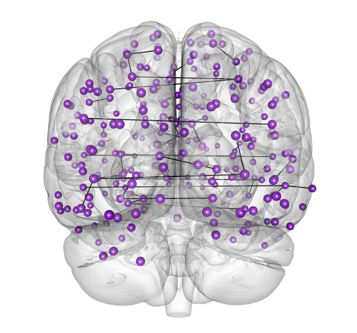
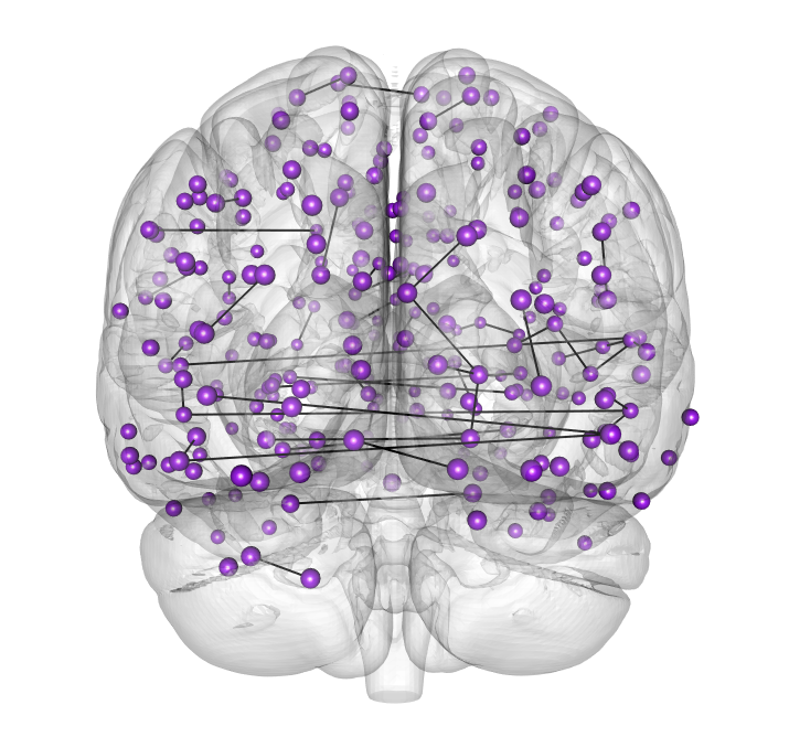
Figure 7: Coronal, sagittal, and transverse snapshots of the difference between our proposal and that of [24]. Panels (a–c) are coronal, sagittal, and transverse snapshots for children and panels (d–f) are coronal, sagittal, and transverse snapshots for adolescent.

We compare our proposed method to [24], which ignores both correlated replicates and unmeasured confounders. We apply [24] by treating replicates as independent subjects. We select the tuning parameter for Meinshausen & Bühlmann 2006 to yield 155 and 159 edges for children and adolescent, respectively. We compare the estimated graphs obtained from our proposed method to that of Meinshausen & Bühlmann 2006 for both the children and adolescent datasets. The difference between the two estimated graphs are plotted in Figure 7. The estimated graphs between the two methods are drastically different for both children and adolescents. In particular, out of approximately 160 total number of edges, 50 edges are different between the two methods for both children and adolescents graphs. Our results suggest that the potential bias introduced by the correlation across replicates and unmeasured confounders can be large, and care must be taken when estimating a conditional dependence graph.

Appendix A Technical Lemmas

We first provide some technical lemmas to facilitate the proof of Theorem 1–2. Lemmas 1 and 2 control the tail behavior of interaction terms between the observed variable and the random noise ϵi​t​j\epsilon_{itj}. The proof of Lemma 1 is provided in Section C.1. The proof of Lemma 2 is similar to Lemma 1 and is omitted. Recall from Section 4 that Xi​t​j∼N⁡(μi​t​j,σj​j,t2)X_{itj}\sim N(\mu_{itj},\sigma_{jj,t}^{2}) with |μi​t​j|≤μm|\mu_{itj}|\leq\mu_{m} and (σmX)2=maxj,t⁡(σj​j,t2)(\sigma_{m}^{X})^{2}=\max_{j,t}(\sigma_{jj,t}^{2}). Besides, let ϵi​t​j∼N⁡{0,(σj​j,tϵ)2}\epsilon_{itj}\sim N\{0,(\sigma_{jj,t}^{\epsilon})^{2}\} and (σmϵ)2=maxj,t⁡{(σj​j,tϵ)2}(\sigma_{m}^{\epsilon})^{2}=\max_{j,t}\{(\sigma_{jj,t}^{\epsilon})^{2}\}.

Lemma 1.

Assume Xi​t​j∼N⁡(μi​t​j,σj​j,t2)X_{itj}\sim N(\mu_{itj},\sigma_{jj,t}^{2}) and ϵi​t​j∼N⁡{0,(σj​j,tϵ)2}\epsilon_{itj}\sim N\{0,(\sigma_{jj,t}^{\epsilon})^{2}\}. We have

max1≤k≤p,k≠j​1n​T​|∑i=1n∑t=1Tϵi​t​j​Xi​t​k|≤λ0,\underset{1\leq k\leq p,k\neq j}{\max}~\frac{1}{nT}\left|\sum_{i=1}^{n}\sum_{t=1}^{T}\epsilon_{itj}X_{itk}\right|\leq\lambda_{0},

with probability at least 1−exp(−min[log2(T)/{2σmϵμm2+(σmX)2}2,log(T)/|2σmϵμm2+(σmX)2|]/2)−exp[log{2(p−1)}−3λ02nT/{2λ0log(T)+6log2(T)}]1-\exp(-\min[\log^{2}(T)/\{2\sigma_{m}^{\epsilon}\sqrt{\mu_{m}^{2}+(\sigma_{m}^{X})^{2}}\}^{2},\log(T)/|2\sigma_{m}^{\epsilon}\sqrt{\mu_{m}^{2}+(\sigma_{m}^{X})^{2}}|]/2)-\exp[\log\{2(p-1)\}-3\lambda_{0}^{2}nT/\{2\lambda_{0}\log(T)+6\log^{2}(T)\}].

Lemma 2.

Assume Xi⁡(t−1)​k∼N⁡(μi⁡(t−1)​k,σk​k,t−12)X_{i(t-1)k}\sim N(\mu_{i(t-1)k},\sigma_{kk,t-1}^{2}) and ϵi​t​j∼N⁡{0,(σj​j,tϵ)2}\epsilon_{itj}\sim N\{0,(\sigma_{jj,t}^{\epsilon})^{2}\}. We have

max1≤k≤p​1n​T​|∑i=1n∑t=1Tϵi​t​j​Xi⁡(t−1)​k|≤β0,\underset{1\leq k\leq p}{\max}~\frac{1}{nT}\left|\sum_{i=1}^{n}\sum_{t=1}^{T}\epsilon_{itj}X_{i(t-1)k}\right|\leq\beta_{0},

with probability at least 1−exp(−min[log2(T)/{2σmϵμm2+(σmX)2}2,log(T)/|2σmϵμm2+(σmX)2|]/2)−exp[log(2p)−3β02nT/{2β0log(T)+6log2(T)}]1-\exp(-\min[\log^{2}(T)/\{2\sigma_{m}^{\epsilon}\sqrt{\mu_{m}^{2}+(\sigma_{m}^{X})^{2}}\}^{2},\log(T)/|2\sigma_{m}^{\epsilon}\sqrt{\mu_{m}^{2}+(\sigma_{m}^{X})^{2}}|]/2)-\exp[\log(2p)-3\beta_{0}^{2}nT/\{2\beta_{0}\log(T)+6\log^{2}(T)\}].

Lemma 3 establishes upper bounds for terms related to 𝚫i​j\bm{\Delta}_{ij}. The proof is provided in Section C.2.

Lemma 3.

Let 𝛈∼N⁡(𝟎,𝐐)\bm{\eta}\sim N\left(\bm{0},\mathbf{Q}\right) and D=8​T​log⁡(T)/(π2​i0)D=8\sqrt{T\log(T)/(\pi^{2}i_{0})}. For i0∈{1,…,T−1}i_{0}\in\{1,\ldots,T-1\}, we have

1n​T​𝜼T​(𝚫¯i​j−𝚫i​j)≤2​‖𝐐‖op​{i0+log⁡(T)}n​T​‖𝚫¯i​j−𝚫i​j‖2+‖𝐐‖op​Dn​T​(‖𝐂​𝚫¯i​j‖1+‖𝐂​𝚫i​j‖1),\frac{1}{nT}\bm{\eta}^{\mathrm{\scriptstyle T}}\left(\bar{\bm{\Delta}}_{ij}-\bm{\Delta}_{ij}\right)\leq\frac{\sqrt{2\big\|\mathbf{Q}\big\|_{\mathrm{op}}}\left\{\sqrt{i_{0}}+\sqrt{\log\left(T\right)}\right\}}{nT}\big\|\bar{\bm{\Delta}}_{ij}-\bm{\Delta}_{ij}\big\|_{2}+\frac{\sqrt{\big\|\mathbf{Q}\big\|_{\mathrm{op}}}D}{nT}\left(\big\|\mathbf{C}\bar{\bm{\Delta}}_{ij}\big\|_{1}+\big\|\mathbf{C}\bm{\Delta}_{ij}\big\|_{1}\right),

with probability at least 1−{2​(T−1)​log⁡(T−1)}−1−2​exp⁡(−i0)−1/{T​2​log⁡(T)}1-\{2(T-1)\sqrt{\log(T-1)}\}^{-1}-2\exp(-i_{0})-1/\{T\sqrt{2\log{(T)}}\}, where ‖𝐐‖op\|\mathbf{Q}\|_{\mathrm{op}} is the operator norm of 𝐐\mathbf{Q}.

Appendix B Proof of Theorems

B.1 Proof of Theorem 1

Let 𝜽j,−j∗∈ℝp−1\bm{\theta}_{j,-j}^{*}\in\mathbb{R}^{p-1}, 𝜶j∗∈ℝp\bm{\alpha}_{j}^{*}\in\mathbb{R}^{p}, and 𝚫j∗∈ℝn​T\bm{\Delta}_{j}^{*}\in\mathbb{R}^{nT} be the true underlying parameters, and let 𝜽^j,−j\widehat{\bm{\theta}}_{j,-j}, 𝜶^j\widehat{\bm{\alpha}}_{j}, and 𝚫^j\widehat{\bm{\Delta}}_{j} be the solution obtained from solving (8) under the Gaussian loss. For notational convenience, we write 𝝎j∗={(𝜽j,−j∗)T,(𝜶j∗)T}T\bm{\omega}_{j}^{*}=\{(\bm{\theta}_{j,-j}^{*})^{\mathrm{\scriptstyle T}},(\bm{\alpha}_{j}^{*})^{\mathrm{\scriptstyle T}}\}^{\mathrm{\scriptstyle T}} and 𝝎^j=(𝜽^j,−jT,𝜶^jT)T\widehat{\bm{\omega}}_{j}=(\widehat{\bm{\theta}}_{j,-j}^{\mathrm{\scriptstyle T}},\widehat{\bm{\alpha}}_{j}^{\mathrm{\scriptstyle T}})^{\mathrm{\scriptstyle T}}. Let 𝒮j={k:ωj​k∗≠0}{\mathcal{S}}_{j}=\{k:\omega_{jk}^{*}\neq 0\} be the active set and let sj=|𝒮j|s_{j}=|{\mathcal{S}}_{j}| be the cardinality of 𝒮j{\mathcal{S}}_{j}. To establish an upper bound on the estimation error, we start with defining

N=‖𝜽^j,−j−𝜽j,−j∗‖1+‖𝜶^j−𝜶j∗‖1+1n​T​‖𝚫^j−𝚫j∗‖2.N=\big\|\widehat{\bm{\theta}}_{j,-j}-\bm{\theta}_{j,-j}^{*}\big\|_{1}+\big\|\widehat{\bm{\alpha}}_{j}-\bm{\alpha}_{j}^{*}\big\|_{1}+\frac{1}{\sqrt{nT}}\big\|\widehat{\bm{\Delta}}_{j}-\bm{\Delta}_{j}^{*}\big\|_{2}.

The goal is to show that N≤MN\leq M, where

M=2​max⁡(c1​n−16​T−13,c2​n−16​T−13+c3​n−12​T−12);c1=4​log⁡(T)​log⁡(n​T​p)​(4​sj+sj​ϕ0)ϕ02;c2=1792​σm2​c443​(μm+1)2log⁡(T)​log⁡(n​T​p)+448​σm​c423;c3=448​σm​log⁡(T)+1792​σm2​{log⁡(T)+2​(μm+1)​c423​log⁡(T)}log⁡(T)​log⁡(n​T​p);c4=[4​log⁡(T)​Δmax2​τ2π2]14.\begin{split}M&=2\max\left(c_{1}n^{-\frac{1}{6}}T^{-\frac{1}{3}},c_{2}n^{-\frac{1}{6}}T^{-\frac{1}{3}}+c_{3}n^{-\frac{1}{2}}T^{-\frac{1}{2}}\right);\\ c_{1}&=\frac{4\log\left(T\right)\log\left(nTp\right)\left(4s_{j}+\sqrt{s_{j}}\phi_{0}\right)}{\phi_{0}^{2}};\\ c_{2}&=\frac{1792\sigma_{m}^{2}c_{4}^{\frac{4}{3}}\left(\mu_{m}+1\right)^{2}}{\log\left(T\right)\log\left(nTp\right)}+448\sigma_{m}c_{4}^{\frac{2}{3}};\\ c_{3}&=448\sigma_{m}\sqrt{\log\left(T\right)}+\frac{1792\sigma_{m}^{2}\left\{\log\left(T\right)+2\left(\mu_{m}+1\right)c_{4}^{\frac{2}{3}}\sqrt{\log\left(T\right)}\right\}}{\log\left(T\right)\log\left(nTp\right)};\\ c_{4}&=\left[\frac{4\log\left(T\right)\Delta_{\max}^{2}\tau^{2}}{\pi^{2}}\right]^{\frac{1}{4}}.\end{split}

Note that the constant ϕ0>0\phi_{0}>0 is the same compatability-type constant that appears in Assumption 4. Let ζ=M/(M+N)\zeta=M/(M+N) such that 0<ζ<10<\zeta<1. Set

𝜽¯j,−j=ζ​𝜽^j,−j+(1−ζ)​𝜽j,−j∗;𝜶¯j=ζ​𝜶^j+(1−ζ)​𝜶j∗;𝚫¯j=ζ​𝚫^j+(1−ζ)​𝚫j∗.\begin{split}\bar{\bm{\theta}}_{j,-j}&=\zeta\widehat{\bm{\theta}}_{j,-j}+(1-\zeta)\bm{\theta}_{j,-j}^{*};\\ \bar{\bm{\alpha}}_{j}&=\zeta\widehat{\bm{\alpha}}_{j}+(1-\zeta)\bm{\alpha}_{j}^{*};\\ \bar{\bm{\Delta}}_{j}&=\zeta\widehat{\bm{\Delta}}_{j}+(1-\zeta)\bm{\Delta}_{j}^{*}.\end{split}

Then, it can be shown that ζ​N=‖𝜽¯j,−j−𝜽j,−j∗‖1+‖𝜶¯j−𝜶j∗‖1+‖𝚫¯j−𝚫j∗‖2/n​T.\zeta N=\big\|\bar{\bm{\theta}}_{j,-j}-\bm{\theta}_{j,-j}^{*}\big\|_{1}+\big\|\bar{\bm{\alpha}}_{j}-\bm{\alpha}_{j}^{*}\big\|_{1}+\big\|\bar{\bm{\Delta}}_{j}-\bm{\Delta}_{j}^{*}\big\|_{2}/\sqrt{nT}. In the following, we show that ζ​N≤M/2\zeta N\leq M/2, which implies N≤MN\leq M.

Let Q⁡(𝝎j,𝚫j)Q\left(\bm{\omega}_{j},\bm{\Delta}_{j}\right) be the loss function in (8) under the assumption that the random variables are Gaussian, that is,

Q⁡(𝝎j,𝚫j)=12​n​T​‖𝐗j−𝐘j​𝝎j−𝚫j‖22+λ​‖𝜽j,−j‖1+β​‖𝜶j‖1+γ​∑i=1n‖𝐂​𝚫i​j‖1,\displaystyle Q\left(\bm{\omega}_{j},\bm{\Delta}_{j}\right)=\frac{1}{2nT}\big\|\mathbf{X}_{j}-\mathbf{Y}_{j}\bm{\omega}_{j}-\bm{\Delta}_{j}\big\|_{2}^{2}+\lambda\big\|\bm{\theta}_{j,-j}\big\|_{1}+\beta\big\|\bm{\alpha}_{j}\big\|_{1}+\gamma\sum_{i=1}^{n}\big\|\mathbf{C}\bm{\Delta}_{ij}\big\|_{1}, (17)

where 𝝎j=(𝜽j,−jT,𝜶jT)T\bm{\omega}_{j}=(\bm{\theta}_{j,-j}^{\mathrm{\scriptstyle T}},\bm{\alpha}_{j}^{\mathrm{\scriptstyle T}})^{\mathrm{\scriptstyle T}}, 𝐘i​t​j=(𝐗i​t​(−j),𝐗i⁡(t−1))\mathbf{Y}_{itj}=(\mathbf{X}_{it(-j)},\mathbf{X}_{i(t-1)}), and 𝐘j=(𝐘11​jT,𝐘12​jT,…,𝐘1​T​jT,𝐘21​jT,…,𝐘n​T​jT)T\mathbf{Y}_{j}=(\mathbf{Y}_{11j}^{\mathrm{\scriptstyle T}},\mathbf{Y}_{12j}^{\mathrm{\scriptstyle T}},\ldots,\mathbf{Y}_{1Tj}^{\mathrm{\scriptstyle T}},\mathbf{Y}_{21j}^{\mathrm{\scriptstyle T}},\ldots,\mathbf{Y}_{nTj}^{\mathrm{\scriptstyle T}})^{\mathrm{\scriptstyle T}}. Since Q⁡(⋅)Q(\cdot) is a convex loss, by convexity, we have

Q⁡(𝝎¯j,𝚫¯j)\displaystyle Q\left(\bar{\bm{\omega}}_{j},\bar{\bm{\Delta}}_{j}\right) =Q⁡{ζ​𝝎^j+(1−ζ)​𝝎j∗,ζ​𝚫^j+(1−ζ)​𝚫j∗}\displaystyle=Q\left\{\zeta\widehat{\bm{\omega}}_{j}+\left(1-\zeta\right)\bm{\omega}_{j}^{*},\zeta\widehat{\bm{\Delta}}_{j}+(1-\zeta)\bm{\Delta}_{j}^{*}\right\}
≤ζ​Q​(𝝎^j,𝚫^j)+(1−ζ)​Q​(𝝎j∗,𝚫j∗)\displaystyle\leq\zeta Q\left(\widehat{\bm{\omega}}_{j},\widehat{\bm{\Delta}}_{j}\right)+\left(1-\zeta\right)Q\left(\bm{\omega}_{j}^{*},\bm{\Delta}_{j}^{*}\right)
≤Q⁡(𝝎j∗,𝚫j∗),\displaystyle\leq Q\left(\bm{\omega}_{j}^{*},\bm{\Delta}_{j}^{*}\right), (18)

where the last inequality follows from the fact that Q⁡(𝝎^j,𝚫^j)≤Q⁡(𝝎j∗,𝚫j∗)Q(\widehat{\bm{\omega}}_{j},\widehat{\bm{\Delta}}_{j})\leq Q(\bm{\omega}_{j}^{*},\bm{\Delta}_{j}^{*}). Substituting (12) and (17) into (B.1), and upon rearranging the terms, we have

12​n​T​‖𝐘j​(𝝎¯j−𝝎j∗)‖22+12​n​T​‖𝚫¯j−𝚫j∗‖22\displaystyle\frac{1}{2nT}\big\|\mathbf{Y}_{j}\left(\bar{\bm{\omega}}_{j}-\bm{\omega}_{j}^{*}\right)\big\|_{2}^{2}+\frac{1}{2nT}\big\|\bar{\bm{\Delta}}_{j}-\bm{\Delta}_{j}^{*}\big\|_{2}^{2}
≤1n​T​ϵjT​𝐘j​(𝝎¯j−𝝎j∗)+λ⁡(‖𝜽j,−j∗‖1−‖𝜽¯j,−j‖1)+β⁡(‖𝜶j∗‖1−‖𝜶¯j‖1)⏟𝕀1\displaystyle\leq\underbrace{\frac{1}{nT}\bm{\epsilon}_{j}^{\mathrm{\scriptstyle T}}\mathbf{Y}_{j}\left(\bar{\bm{\omega}}_{j}-\bm{\omega}_{j}^{*}\right)+\lambda\left(\|\bm{\theta}_{j,-j}^{*}\|_{1}-\|\bar{\bm{\theta}}_{j,-j}\|_{1}\right)+\beta\left(\|\bm{\alpha}_{j}^{*}\|_{1}-\|\bar{\bm{\alpha}}_{j}\|_{1}\right)}_{\mathbb{I}_{1}}
+∑i=1n{1n​T​ϵi​jT​(𝚫¯i​j−𝚫i​j∗)+1n​T​(𝝎¯j−𝝎j∗)T​𝐘i​jT​(𝚫i​j∗−𝚫¯i​j)⏟𝕀2+γ(∥𝐂𝚫i​j∗∥1−∥𝐂𝚫¯i​j∥1)}.\displaystyle+\sum_{i=1}^{n}\left\{\underbrace{\frac{1}{nT}\bm{\epsilon}_{ij}^{\mathrm{\scriptstyle T}}\left(\bar{\bm{\Delta}}_{ij}-\bm{\Delta}_{ij}^{*}\right)+\frac{1}{nT}\left(\bar{\bm{\omega}}_{j}-\bm{\omega}_{j}^{*}\right)^{\mathrm{\scriptstyle T}}\mathbf{Y}_{ij}^{\mathrm{\scriptstyle T}}\left(\bm{\Delta}_{ij}^{*}-\bar{\bm{\Delta}}_{ij}\right)}_{\mathbb{I}_{2}}+\gamma\left(\|\mathbf{C}\bm{\Delta}_{ij}^{*}\|_{1}-\|\mathbf{C}\bar{\bm{\Delta}}_{ij}\|_{1}\right)\right\}. (19)

We now establish upper bounds for 𝕀1\mathbb{I}_{1} and 𝕀2\mathbb{I}_{2}, respectively.

Upper Bound for 𝕀1\mathbb{I}_{1}: from the definition of 𝐘j\mathbf{Y}_{j}, we have

ϵjT​𝐘j​(𝝎¯j−𝝎j∗)=ϵjT​𝐗−j⊗​(𝜽¯j,−j−𝜽j,−j∗)⏟𝕀11+ϵjT​𝐗j⊗​(𝜶¯j−𝜶j∗)⏟𝕀12.\displaystyle\bm{\epsilon}_{j}^{\mathrm{\scriptstyle T}}\mathbf{Y}_{j}(\bar{\bm{\omega}}_{j}-\bm{\omega}_{j}^{*})=\underbrace{\bm{\epsilon}_{j}^{\mathrm{\scriptstyle T}}\mathbf{X}_{-j}^{\otimes}(\bar{\bm{\theta}}_{j,-j}-\bm{\theta}_{j,-j}^{*})}_{\mathbb{I}_{11}}+\underbrace{\bm{\epsilon}_{j}^{\mathrm{\scriptstyle T}}\mathbf{X}_{j}^{\otimes}(\bar{\bm{\alpha}}_{j}-\bm{\alpha}_{j}^{*})}_{\mathbb{I}_{12}}.

It suffices to obtain upper bounds for 𝕀11\mathbb{I}_{11} and 𝕀12\mathbb{I}_{12}. By the Holder’s inequality, Lemma 1, and picking λ=2log(T)log(nTp)n−1/6T−1/3\lambda=2\log(T)\log(nTp)n^{-1/6}T^{-1/3}, when n,T,p≥6n,T,p\geq 6 we have

1n​T​ϵjT​𝐗−j⊗​(𝜽¯j,−j−𝜽j,−j∗)≤1n​T​‖ϵjT​𝐗−j⊗‖∞⋅‖𝜽¯j,−j−𝜽j,−j∗‖1≤λ2​‖𝜽¯j,−j−𝜽j,−j∗‖1,\frac{1}{nT}\bm{\epsilon}_{j}^{\mathrm{\scriptstyle T}}\mathbf{X}_{-j}^{\otimes}\left(\bar{\bm{\theta}}_{j,-j}-\bm{\theta}_{j,-j}^{*}\right)\leq\frac{1}{nT}\big\|\bm{\epsilon}_{j}^{\mathrm{\scriptstyle T}}\mathbf{X}_{-j}^{\otimes}\big\|_{\infty}\cdot\big\|\bar{\bm{\theta}}_{j,-j}-\bm{\theta}_{j,-j}^{*}\big\|_{1}\leq\frac{\lambda}{2}\big\|\bar{\bm{\theta}}_{j,-j}-\bm{\theta}_{j,-j}^{*}\big\|_{1}, (20)

with probability at least 1−exp(−min[log2(T)/{2σmϵμm2+(σmX)2}2,log(T)/|2σmϵμm2+(σmX)2|]/2)−2/(nTp)1-\exp(-\min[\log^{2}(T)/\{2\sigma_{m}^{\epsilon}\sqrt{\mu_{m}^{2}+(\sigma_{m}^{X})^{2}}\}^{2},\log(T)/|2\sigma_{m}^{\epsilon}\sqrt{\mu_{m}^{2}+(\sigma_{m}^{X})^{2}}|]/2)-2/(nTp). Similarly, by an application of Lemma 2 and picking β=λ\beta=\lambda, when n,T,p≥6n,T,p\geq 6 we obtain

1n​T​ϵjT​𝐗j⊗​(𝜶¯j−𝜶j∗)≤1n​T​‖ϵjT​𝐗j⊗‖∞⋅‖𝜶¯j−𝜶j∗‖1≤β2​‖𝜶¯j−𝜶j∗‖1,\frac{1}{nT}\bm{\epsilon}_{j}^{\mathrm{\scriptstyle T}}\mathbf{X}_{j}^{\otimes}(\bar{\bm{\alpha}}_{j}-\bm{\alpha}_{j}^{*})\leq\frac{1}{nT}\big\|\bm{\epsilon}_{j}^{\mathrm{\scriptstyle T}}\mathbf{X}_{j}^{\otimes}\big\|_{\infty}\cdot\|\bar{\bm{\alpha}}_{j}-\bm{\alpha}_{j}^{*}\|_{1}\leq\frac{\beta}{2}\|\bar{\bm{\alpha}}_{j}-\bm{\alpha}_{j}^{*}\|_{1}, (21)

with probability at least 1−exp(−min[log2(T)/{2σmϵμm2+(σmX)2}2,log(T)/|2σmϵμm2+(σmX)2|]/2)−2/(nTp)1-\exp(-\min[\log^{2}(T)/\{2\sigma_{m}^{\epsilon}\sqrt{\mu_{m}^{2}+(\sigma_{m}^{X})^{2}}\}^{2},\log(T)/|2\sigma_{m}^{\epsilon}\sqrt{\mu_{m}^{2}+(\sigma_{m}^{X})^{2}}|]/2)-2/(nTp). Since λ=β\lambda=\beta, substituting (20) and (21) into 𝕀1\mathbb{I}_{1} yields

𝕀1≤β2​‖𝝎¯j−𝝎j∗‖1+β⁡(‖𝝎j∗‖1−‖𝝎¯j‖1),\displaystyle\mathbb{I}_{1}\leq\frac{\beta}{2}\|\bar{\bm{\omega}}_{j}-\bm{\omega}_{j}^{*}\|_{1}+\beta\left(\|\bm{\omega}_{j}^{*}\|_{1}-\|\bar{\bm{\omega}}_{j}\|_{1}\right), (22)

with probability at least 1−2exp(−min[log2(T)/{2σmϵμm2+(σmX)2}2,log(T)/|2σmϵμm2+(σmX)2|]/2)−4/(nTp)1-2\exp(-\min[\log^{2}(T)/\{2\sigma_{m}^{\epsilon}\sqrt{\mu_{m}^{2}+(\sigma_{m}^{X})^{2}}\}^{2},\log(T)/|2\sigma_{m}^{\epsilon}\sqrt{\mu_{m}^{2}+(\sigma_{m}^{X})^{2}}|]/2)-4/(nTp). Let 𝝎j𝒮j\bm{\omega}_{j}^{{\mathcal{S}}_{j}} and 𝝎j𝒮jc\bm{\omega}_{j}^{{\mathcal{S}}_{j}^{c}} be subvectors of 𝝎j\bm{\omega}_{j} with indices 𝒮j{\mathcal{S}}_{j} and 𝒮jc{\mathcal{S}}_{j}^{c}, respectively. Then, upon rearranging the terms, (22) can be rewritten as

𝕀1≤3​β2​‖𝝎¯j𝒮j−(𝝎j∗)𝒮j‖1−β2​‖𝝎¯j𝒮jc‖1,\displaystyle\mathbb{I}_{1}\leq\frac{3\beta}{2}\left\|\bar{\bm{\omega}}_{j}^{{\mathcal{S}}_{j}}-(\bm{\omega}_{j}^{*})^{{\mathcal{S}}_{j}}\right\|_{1}-\frac{\beta}{2}\left\|\bar{\bm{\omega}}_{j}^{{\mathcal{S}}_{j}^{c}}\right\|_{1}, (23)

with probability at least 1−2exp(−min[log2(T)/{2σmϵμm2+(σmX)2}2,log(T)/|2σmϵμm2+(σmX)2|]/2)−4/(nTp)1-2\exp(-\min[\log^{2}(T)/\{2\sigma_{m}^{\epsilon}\sqrt{\mu_{m}^{2}+(\sigma_{m}^{X})^{2}}\}^{2},\log(T)/|2\sigma_{m}^{\epsilon}\sqrt{\mu_{m}^{2}+(\sigma_{m}^{X})^{2}}|]/2)-4/(nTp).

Upper Bound for 𝕀2\mathbb{I}_{2}: we start with providing an upper bound for ϵi​jT​(𝚫¯i​j−𝚫i​j∗)/(n​T)\bm{\epsilon}_{ij}^{\mathrm{\scriptstyle T}}(\bar{\bm{\Delta}}_{ij}-\bm{\Delta}_{ij}^{*})/(nT). For i0∈{1,…,T−1}i_{0}\in\{1,\ldots,T-1\}, let D=8​T​log⁡(T)/(π2​i0)D=8\sqrt{T\log(T)/(\pi^{2}i_{0})}. Recall that ϵi​t​j∼N⁡{0,(σt​jϵ)2}\epsilon_{itj}\sim N\{0,(\sigma^{\epsilon}_{tj})^{2}\} and (σmϵ)2=maxt,j⁡{(σt​jϵ)2}(\sigma^{\epsilon}_{m})^{2}=\max_{t,j}\{(\sigma^{\epsilon}_{tj})^{2}\}. By Lemma 3, we have

1n​T​ϵi​jT​(𝚫¯i​j−𝚫i​j∗)≤2​σmϵ​{i0+log⁡(T)}n​T​‖𝚫¯i​j−𝚫i​j∗‖2+σmϵ​Dn​T​(‖𝐂​𝚫¯i​j‖1+‖𝐂​𝚫i​j∗‖1),\displaystyle\frac{1}{nT}\bm{\epsilon}_{ij}^{\mathrm{\scriptstyle T}}\left(\bar{\bm{\Delta}}_{ij}-\bm{\Delta}_{ij}^{*}\right)\leq\frac{\sqrt{2}\sigma^{\epsilon}_{m}\left\{\sqrt{i_{0}}+\sqrt{\log\left(T\right)}\right\}}{nT}\big\|\bar{\bm{\Delta}}_{ij}-\bm{\Delta}_{ij}^{*}\big\|_{2}+\frac{\sigma^{\epsilon}_{m}D}{nT}\left(\big\|\mathbf{C}\bar{\bm{\Delta}}_{ij}\big\|_{1}+\big\|\mathbf{C}\bm{\Delta}_{ij}^{*}\big\|_{1}\right), (24)

with probability at least 1−{2​(T−1)​log⁡(T−1)}−1−2​exp⁡(−i0)−1/{T​2​log⁡(T)}1-\{2(T-1)\sqrt{\log(T-1)}\}^{-1}-2\exp(-i_{0})-1/\{T\sqrt{2\log{(T)}}\}.

Next, we provide an upper bound for (𝝎¯j−𝝎j∗)T​𝐘i​jT​(𝚫i​j∗−𝚫¯i​j)/(n​T)(\bar{\bm{\omega}}_{j}-\bm{\omega}_{j}^{*})^{\mathrm{\scriptstyle T}}\mathbf{Y}_{ij}^{\mathrm{\scriptstyle T}}(\bm{\Delta}_{ij}^{*}-\bar{\bm{\Delta}}_{ij})/(nT) in 𝕀2\mathbb{I}_{2}. Let 𝔼⁡(𝐘i​j)=𝐔i​j\mathbb{E}(\mathbf{Y}_{ij})=\mathbf{U}_{ij} and B⁡(n,T)=μm​min⁡(c42/3​n1/3​T1/6,T)B(n,T)=\mu_{m}\min(c_{4}^{2/3}n^{1/3}T^{1/6},\sqrt{T}). By Assumption 3, ‖𝝁i​j‖2≤B⁡(n,T)\|\bm{\mu}_{ij}\|_{2}\leq B(n,T). Recall that ‖𝝎¯j−𝝎j∗‖1+‖𝚫¯j−𝚫j∗‖2/n​T=ζ​N≤M\|\bar{\bm{\omega}}_{j}-\bm{\omega}_{j}^{*}\|_{1}+\|\bar{\bm{\Delta}}_{j}-\bm{\Delta}_{j}^{*}\|_{2}/\sqrt{nT}=\zeta N\leq M with ζ=M/(N+M)\zeta=M/(N+M). This implies that ‖𝝎¯j−𝝎j∗‖1≤M\big\|\bar{\bm{\omega}}_{j}-\bm{\omega}_{j}^{*}\big\|_{1}\leq M. Coupling the above with the Holder’s inequality, we obtain

1n​T​(𝝎¯j−𝝎j∗)T​𝐘i​jT​(𝚫i​j∗−𝚫¯i​j)≤1n​T​‖𝝎¯j−𝝎j∗‖1⋅‖𝐘i​jT​(𝚫i​j∗−𝚫¯i​j)‖∞≤Mn​T​‖𝐘i​jT​(𝚫i​j∗−𝚫¯i​j)‖∞≤Mn​T​‖(𝐘i​j−𝐔i​j)T​(𝚫i​j∗−𝚫¯i​j)‖∞+Mn​T​‖𝐔i​jT​(𝚫i​j∗−𝚫¯i​j)‖∞≤Mn​T​‖(𝐘i​j−𝐔i​j)T​(𝚫i​j∗−𝚫¯i​j)‖∞+Mn​T​maxk≠j​‖𝝁i​k‖2​‖𝚫i​j∗−𝚫¯i​j‖2≤M​2​κ​{i0+log⁡(T)+B⁡(n,T)}n​T​‖𝚫¯i​j−𝚫i​j∗‖2+M​κ​Dn​T​(‖𝐂​𝚫¯i​j‖1+‖𝐂​𝚫i​j∗‖1),\begin{split}&\frac{1}{nT}\left(\bar{\bm{\omega}}_{j}-\bm{\omega}_{j}^{*}\right)^{\mathrm{\scriptstyle T}}\mathbf{Y}_{ij}^{\mathrm{\scriptstyle T}}\left(\bm{\Delta}_{ij}^{*}-\bar{\bm{\Delta}}_{ij}\right)\\ &\leq\frac{1}{nT}\big\|\bar{\bm{\omega}}_{j}-\bm{\omega}_{j}^{*}\big\|_{1}\cdot\big\|\mathbf{Y}_{ij}^{\mathrm{\scriptstyle T}}\left(\bm{\Delta}_{ij}^{*}-\bar{\bm{\Delta}}_{ij}\right)\big\|_{\infty}\\ &\leq\frac{M}{nT}\big\|\mathbf{Y}_{ij}^{\mathrm{\scriptstyle T}}\left(\bm{\Delta}_{ij}^{*}-\bar{\bm{\Delta}}_{ij}\right)\big\|_{\infty}\\ &\leq\frac{M}{nT}\big\|\left(\mathbf{Y}_{ij}-\mathbf{U}_{ij}\right)^{\mathrm{\scriptstyle T}}\left(\bm{\Delta}_{ij}^{*}-\bar{\bm{\Delta}}_{ij}\right)\big\|_{\infty}+\frac{M}{nT}\big\|\mathbf{U}_{ij}^{\mathrm{\scriptstyle T}}\left(\bm{\Delta}_{ij}^{*}-\bar{\bm{\Delta}}_{ij}\right)\big\|_{\infty}\\ &\leq\frac{M}{nT}\big\|\left(\mathbf{Y}_{ij}-\mathbf{U}_{ij}\right)^{\mathrm{\scriptstyle T}}\left(\bm{\Delta}_{ij}^{*}-\bar{\bm{\Delta}}_{ij}\right)\big\|_{\infty}+\frac{M}{nT}\max_{k\neq j}\big\|\bm{\mu}_{ik}\big\|_{2}\big\|\bm{\Delta}_{ij}^{*}-\bar{\bm{\Delta}}_{ij}\big\|_{2}\\ &\leq\frac{M\sqrt{2\kappa}\left\{\sqrt{i_{0}}+\sqrt{\log\left(T\right)}+B\left(n,T\right)\right\}}{nT}\big\|\bar{\bm{\Delta}}_{ij}-\bm{\Delta}_{ij}^{*}\big\|_{2}+\frac{M\sqrt{\kappa}D}{nT}\left(\big\|\mathbf{C}\bar{\bm{\Delta}}_{ij}\big\|_{1}+\big\|\mathbf{C}\bm{\Delta}_{ij}^{*}\big\|_{1}\right),\end{split} (25)

with probability at least 1−{2​(T−1)​log⁡(T−1)}−1−2​exp⁡(−i0)−1/{T​2​log⁡(T)}1-\{2(T-1)\sqrt{\log(T-1)}\}^{-1}-2\exp(-i_{0})-1/\{T\sqrt{2\log{(T)}}\}. Note that the last inequality follows by an application of Lemma 3, Assumption 3, and the fact that ‖(𝐘i​j−𝐔i​j)T​(𝚫i​j∗−𝚫¯i​j)‖∞=maxk≠{j,j+2​p}​𝒀~i​kT​(𝚫i​j∗−𝚫¯i​j)\|(\mathbf{Y}_{ij}-\mathbf{U}_{ij})^{\mathrm{\scriptstyle T}}(\bm{\Delta}_{ij}^{*}-\bar{\bm{\Delta}}_{ij})\|_{\infty}=\underset{k\neq\{j,j+2p\}}{\max}~\widetilde{\bm{Y}}_{ik}^{\mathrm{\scriptstyle T}}(\bm{\Delta}_{ij}^{*}-\bar{\bm{\Delta}}_{ij}), where 𝒀~i​k\widetilde{\bm{Y}}_{ik} is the kkth column of {(𝐘i​j−𝐔i​j),−(𝐘i​j−𝐔i​j)}\{(\mathbf{Y}_{ij}-\mathbf{U}_{ij}),-(\mathbf{Y}_{ij}-\mathbf{U}_{ij})\}. Let σm=max⁡{2​κ,2​σmϵ,1}\sigma_{m}=\max\{\sqrt{2\kappa},\sqrt{2}\sigma_{m}^{\epsilon},1\}. By (24) and (25), we have

𝕀2≤(M+1)​{i0+log⁡(T)+B⁡(n,T)}​σmn​T​‖𝚫¯i​j−𝚫i​j∗‖2+(M+1)​σm​Dn​T​(‖𝐂​𝚫i​j∗‖1+‖𝐂​𝚫¯i​j‖1),\mathbb{I}_{2}\leq\frac{\left(M+1\right)\left\{\sqrt{i_{0}}+\sqrt{\log\left(T\right)}+B\left(n,T\right)\right\}\sigma_{m}}{nT}\big\|\bar{\bm{\Delta}}_{ij}-\bm{\Delta}_{ij}^{*}\big\|_{2}+\frac{\left(M+1\right)\sigma_{m}D}{nT}\left(\big\|\mathbf{C}\bm{\Delta}_{ij}^{*}\big\|_{1}+\big\|\mathbf{C}\bar{\bm{\Delta}}_{ij}\big\|_{1}\right), (26)

with probability at least 1−{2​(T−1)​log⁡(T−1)}−1−2​exp⁡(−i0)−1/{T​2​log⁡(T)}1-\{2(T-1)\sqrt{\log(T-1)}\}^{-1}-2\exp(-i_{0})-1/\{T\sqrt{2\log{(T)}}\}.

Under the condition that 2max(c1n−1/6T−1/3,c2n−1/6T−1/3+c3n−1/2T−1/2)≤12\max(c_{1}n^{-1/6}T^{-1/3},c_{2}n^{-1/6}T^{-1/3}+c_{3}n^{-1/2}T^{-1/2})\leq 1, we have M≤1M\leq 1. Moreover, recall that γ\gamma is the tuning parameter for ‖(𝐈n⊗𝐂)​𝚫j∗‖1\|(\mathbf{I}_{n}\otimes\mathbf{C})\bm{\Delta}_{j}^{*}\|_{1}. Let γ=2​σm​D/(n​T)\gamma=2\sigma_{m}D/(nT) and substituting (23) and (26) into (B.1), we have

12​n​T​‖𝐘j​(𝝎¯j−𝝎j∗)‖22+12​n​T​‖𝚫¯j−𝚫j∗‖22+β2​‖𝝎¯j𝒮jc‖\displaystyle\frac{1}{2nT}\big\|\mathbf{Y}_{j}\left(\bar{\bm{\omega}}_{j}-\bm{\omega}_{j}^{*}\right)\big\|_{2}^{2}+\frac{1}{2nT}\big\|\bar{\bm{\Delta}}_{j}-\bm{\Delta}_{j}^{*}\big\|_{2}^{2}+\frac{\beta}{2}\big\|\bar{\bm{\omega}}_{j}^{{\mathcal{S}}_{j}^{c}}\big\|
≤3​β2​‖𝝎¯j𝒮j−(𝝎j∗)𝒮j‖1+2​σm​{i0+log⁡(T)}+B⁡(n,T)n​T​‖𝚫¯j−𝚫j∗‖2+4​σm​Dn​T​‖(𝐈n⊗𝐂)​𝚫j∗‖1,\displaystyle\leq\frac{3\beta}{2}\big\|\bar{\bm{\omega}}_{j}^{{\mathcal{S}}_{j}}-(\bm{\omega}_{j}^{*})^{{\mathcal{S}}_{j}}\big\|_{1}+\frac{2\sigma_{m}\left\{\sqrt{i_{0}}+\sqrt{\log\left(T\right)}\right\}+B\left(n,T\right)}{nT}\big\|\bar{\bm{\Delta}}_{j}-\bm{\Delta}_{j}^{*}\big\|_{2}+\frac{4\sigma_{m}D}{nT}\big\|\left(\mathbf{I}_{n}\otimes\mathbf{C}\right)\bm{\Delta}_{j}^{*}\big\|_{1}, (27)

with probability at least 1−{2(T−1)log⁡(T−1)}−1−2exp(−i0)−1/{T2​log⁡(T)}−4/(nTp)−exp(−min[log2(T)/{2σmϵμm2+(σmX)2}2,log(T)/|2σmϵμm2+(σmX)2|]/2)1-\{2(T-1)\sqrt{\log(T-1)}\}^{-1}-2\exp(-i_{0})-1/\{T\sqrt{2\log{(T)}}\}-4/(nTp)-\exp(-\min[\log^{2}(T)/\{2\sigma_{m}^{\epsilon}\sqrt{\mu_{m}^{2}+(\sigma_{m}^{X})^{2}}\}^{2},\log(T)/|2\sigma_{m}^{\epsilon}\sqrt{\mu_{m}^{2}+(\sigma_{m}^{X})^{2}}|]/2).

We now consider (B.1) under the following two cases:

  1. (i)

    2​σm​{i0+log⁡(T)+B⁡(n,T)}n​T​‖𝚫¯j−𝚫j∗‖2+4​σm​Dn​T​‖(𝐈n⊗𝐂)​𝚫j∗‖1≤14​β​‖𝝎¯j−𝝎j∗‖1\frac{2\sigma_{m}\left\{\sqrt{i_{0}}+\sqrt{\log\left(T\right)}+B\left(n,T\right)\right\}}{nT}\big\|\bar{\bm{\Delta}}_{j}-\bm{\Delta}_{j}^{*}\big\|_{2}+\frac{4\sigma_{m}D}{nT}\big\|\left(\mathbf{I}_{n}\otimes\mathbf{C}\right)\bm{\Delta}_{j}^{*}\big\|_{1}\leq\frac{1}{4}\beta\big\|\bar{\bm{\omega}}_{j}-\bm{\omega}_{j}^{*}\big\|_{1};

  2. (ii)

    2​σm​{i0+log⁡(T)+B⁡(n,T)}n​T​‖𝚫¯j−𝚫j∗‖2+4​σm​Dn​T​‖(𝐈n⊗𝐂)​𝚫j∗‖1>14​β​‖𝝎¯j−𝝎j∗‖1\frac{2\sigma_{m}\left\{\sqrt{i_{0}}+\sqrt{\log\left(T\right)}+B\left(n,T\right)\right\}}{nT}\big\|\bar{\bm{\Delta}}_{j}-\bm{\Delta}_{j}^{*}\big\|_{2}+\frac{4\sigma_{m}D}{nT}\big\|\left(\mathbf{I}_{n}\otimes\mathbf{C}\right)\bm{\Delta}_{j}^{*}\big\|_{1}>\frac{1}{4}\beta\big\|\bar{\bm{\omega}}_{j}-\bm{\omega}_{j}^{*}\big\|_{1}.

Recall that ζ​N=‖𝝎¯j−𝝎j∗‖1+‖𝚫¯j−𝚫j∗‖2/n​T\zeta N=\|\bar{\bm{\omega}}_{j}-\bm{\omega}_{j}^{*}\|_{1}+\|\bar{\bm{\Delta}}_{j}-\bm{\Delta}_{j}^{*}\|_{2}/\sqrt{nT} and the goal is to obtain ζ​N≤M/2\zeta N\leq M/2. To this end, we will derive upper bounds for ‖𝝎¯j−𝝎j∗‖1\|\bar{\bm{\omega}}_{j}-\bm{\omega}_{j}^{*}\|_{1} and ‖𝚫¯j−𝚫j∗‖2/n​T\|\bar{\bm{\Delta}}_{j}-\bm{\Delta}_{j}^{*}\|_{2}/\sqrt{nT} separately.

Case (i): in this case, (B.1) can be simplified to

12​n​T​‖𝐘j​(𝝎¯j−𝝎j∗)‖22+12​n​T​‖𝚫¯j−𝚫j∗‖22+β4​‖𝝎¯j𝒮jc‖≤7​β4​‖𝝎¯j𝒮j−(𝝎j∗)𝒮j‖1.\displaystyle\frac{1}{2nT}\big\|\mathbf{Y}_{j}\left(\bar{\bm{\omega}}_{j}-\bm{\omega}_{j}^{*}\right)\big\|_{2}^{2}+\frac{1}{2nT}\big\|\bar{\bm{\Delta}}_{j}-\bm{\Delta}_{j}^{*}\big\|_{2}^{2}+\frac{\beta}{4}\big\|\bar{\bm{\omega}}_{j}^{{\mathcal{S}}_{j}^{c}}\big\|\leq\frac{7\beta}{4}\big\|\bar{\bm{\omega}}_{j}^{{\mathcal{S}}_{j}}-(\bm{\omega}_{j}^{*})^{{\mathcal{S}}_{j}}\big\|_{1}. (28)

Since ‖𝝎¯j−𝝎j∗‖1=‖𝝎¯j𝒮j−(𝝎j∗)𝒮j‖1+‖𝝎¯j𝒮jc‖1\|\bar{\bm{\omega}}_{j}-\bm{\omega}_{j}^{*}\|_{1}=\|\bar{\bm{\omega}}_{j}^{{\mathcal{S}}_{j}}-(\bm{\omega}_{j}^{*})^{{\mathcal{S}}_{j}}\|_{1}+\|\bar{\bm{\omega}}_{j}^{{\mathcal{S}}_{j}^{c}}\|_{1}, following an argument similar to Lemma 6.3 in [6], we have

2n​T​‖𝐘j​(𝝎¯j−𝝎j∗)‖22+2n​T​‖𝚫¯j−𝚫j∗‖22+β​‖𝝎¯j−𝝎j∗‖1\displaystyle\frac{2}{nT}\big\|\mathbf{Y}_{j}\left(\bar{\bm{\omega}}_{j}-\bm{\omega}_{j}^{*}\right)\big\|_{2}^{2}+\frac{2}{nT}\big\|\bar{\bm{\Delta}}_{j}-\bm{\Delta}_{j}^{*}\big\|_{2}^{2}+\beta\big\|\bar{\bm{\omega}}_{j}-\bm{\omega}_{j}^{*}\big\|_{1}
=2n​T​‖𝐘j​(𝝎¯j−𝝎j∗)‖22+2n​T​‖𝚫¯j−𝚫j∗‖22+β​‖𝝎¯j𝒮j−(𝝎j∗)𝒮j‖1+β​‖𝝎¯j𝒮jc‖1\displaystyle=\frac{2}{nT}\big\|\mathbf{Y}_{j}\left(\bar{\bm{\omega}}_{j}-\bm{\omega}_{j}^{*}\right)\big\|_{2}^{2}+\frac{2}{nT}\big\|\bar{\bm{\Delta}}_{j}-\bm{\Delta}_{j}^{*}\big\|_{2}^{2}+\beta\big\|\bar{\bm{\omega}}_{j}^{{\mathcal{S}}_{j}}-(\bm{\omega}_{j}^{*})^{{\mathcal{S}}_{j}}\big\|_{1}+\beta\big\|\bar{\bm{\omega}}_{j}^{{\mathcal{S}}_{j}^{c}}\big\|_{1}
≤8​β​‖𝝎¯j𝒮j−(𝝎j∗)𝒮j‖1\displaystyle\leq 8\beta\big\|\bar{\bm{\omega}}_{j}^{{\mathcal{S}}_{j}}-(\bm{\omega}_{j}^{*})^{{\mathcal{S}}_{j}}\big\|_{1}
≤8​β​sjϕ0​n​T​‖𝐘j​(𝝎¯j−𝝎j∗)‖2\displaystyle\leq\frac{8\beta\sqrt{s_{j}}}{\phi_{0}\sqrt{nT}}\big\|\mathbf{Y}_{j}\left(\bar{\bm{\omega}}_{j}-\bm{\omega}_{j}^{*}\right)\big\|_{2}
≤2n​T​‖𝐘j​(𝝎¯j−𝝎j∗)‖22+8​β2​sjϕ02,\displaystyle\leq\frac{2}{nT}\big\|\mathbf{Y}_{j}\left(\bar{\bm{\omega}}_{j}-\bm{\omega}_{j}^{*}\right)\big\|_{2}^{2}+\frac{8\beta^{2}s_{j}}{\phi_{0}^{2}}, (29)

where ϕ0\phi_{0} is a compatibility-type constant introduced in Assumption 4. The first inequality follows from (28), the second inequality follows from Assumption 4, and the last inequality follows from the fact that u​v≤u2+v2/4uv\leq u^{2}+v^{2}/4 for any u,v≥0u,v\geq 0. Simplifying (B.1), we obtain

2n​T​‖𝚫¯j−𝚫j∗‖22+β​‖𝝎¯j−𝝎j∗‖1≤8​β2​sjϕ02,\frac{2}{nT}\big\|\bar{\bm{\Delta}}_{j}-\bm{\Delta}_{j}^{*}\big\|_{2}^{2}+\beta\big\|\bar{\bm{\omega}}_{j}-\bm{\omega}_{j}^{*}\big\|_{1}\leq\frac{8\beta^{2}s_{j}}{\phi_{0}^{2}},

which directly implies ‖𝝎¯j−𝝎j∗‖1≤8​β​sj/ϕ02\|\bar{\bm{\omega}}_{j}-\bm{\omega}_{j}^{*}\|_{1}\leq 8\beta s_{j}/\phi_{0}^{2} and ‖𝚫¯j−𝚫j∗‖2/n​T≤2​β​sj/ϕ0\|\bar{\bm{\Delta}}_{j}-\bm{\Delta}_{j}^{*}\|_{2}/\sqrt{nT}\leq 2\beta\sqrt{s_{j}}/\phi_{0}. Recall that β=2log(T)log(nTp)n−1/6T−1/3\beta=2\log(T)\log(nTp)n^{-1/6}T^{-1/3}, and thus we have

ζ​N=‖𝝎¯j−𝝎j∗‖1+1n​T​‖𝚫¯j−𝚫j∗‖2≤c1​n−16​T−13,\displaystyle\zeta N=\big\|\bar{\bm{\omega}}_{j}-\bm{\omega}_{j}^{*}\big\|_{1}+\frac{1}{\sqrt{nT}}\big\|\bar{\bm{\Delta}}_{j}-\bm{\Delta}_{j}^{*}\big\|_{2}\leq c_{1}n^{-\frac{1}{6}}T^{-\frac{1}{3}}, (30)

where c1=4​log⁡(T)​log⁡(n​T​p)​(4​sj+sj​ϕ0)/ϕ02c_{1}=4\log(T)\log(nTp)(4s_{j}+\sqrt{s_{j}}\phi_{0})/\phi_{0}^{2}.

Case (ii): we first derive the upper bound of ‖𝚫¯j−𝚫j∗‖2/n​T\|\bar{\bm{\Delta}}_{j}-\bm{\Delta}_{j}^{*}\|_{2}/\sqrt{nT}. From the condition of case (ii), we have

3​β2​‖𝝎¯j𝒮j−(𝝎j∗)𝒮j‖1<12​σm​{i0+log⁡(T)+B⁡(n,T)}n​T​‖𝚫¯j−𝚫j∗‖2+24​σm​Dn​T​‖(𝐈n⊗𝐂)​𝚫j∗‖1.\displaystyle\frac{3\beta}{2}\big\|\bar{\bm{\omega}}_{j}^{{\mathcal{S}}_{j}}-(\bm{\omega}_{j}^{*})^{{\mathcal{S}}_{j}}\big\|_{1}<\frac{12\sigma_{m}\left\{\sqrt{i_{0}}+\sqrt{\log\left(T\right)}+B\left(n,T\right)\right\}}{nT}\big\|\bar{\bm{\Delta}}_{j}-\bm{\Delta}_{j}^{*}\big\|_{2}+\frac{24\sigma_{m}D}{nT}\big\|\left(\mathbf{I}_{n}\otimes\mathbf{C}\right)\bm{\Delta}_{j}^{*}\big\|_{1}. (31)

From (B.1), we obtain

12​n​T​‖𝚫¯j−𝚫j∗‖22≤\displaystyle\frac{1}{2nT}\big\|\bar{\bm{\Delta}}_{j}-\bm{\Delta}_{j}^{*}\big\|_{2}^{2}\leq 3​β2​‖𝝎¯j𝒮j−(𝝎j∗)𝒮j‖1+2​σm​{i0+log⁡(T)+B⁡(n,T)}n​T​‖𝚫¯j−𝚫j∗‖2\displaystyle\frac{3\beta}{2}\big\|\bar{\bm{\omega}}_{j}^{{\mathcal{S}}_{j}}-(\bm{\omega}_{j}^{*})^{{\mathcal{S}}_{j}}\big\|_{1}+\frac{2\sigma_{m}\left\{\sqrt{i_{0}}+\sqrt{\log\left(T\right)}+B\left(n,T\right)\right\}}{nT}\big\|\bar{\bm{\Delta}}_{j}-\bm{\Delta}_{j}^{*}\big\|_{2}
+4​σm​Dn​T​‖(𝐈n⊗𝐂)​𝚫j∗‖1.\displaystyle+\frac{4\sigma_{m}D}{nT}\big\|\left(\mathbf{I}_{n}\otimes\mathbf{C}\right)\bm{\Delta}_{j}^{*}\big\|_{1}. (32)

Substituting (31) into (B.1), we have

‖𝚫¯j−𝚫j∗‖22≤28​σm​{i0+log⁡(T)+B⁡(n,T)}​‖𝚫¯j−𝚫j∗‖2+56​σm​D​‖(𝐈n⊗𝐂)​𝚫j∗‖1.\displaystyle\big\|\bar{\bm{\Delta}}_{j}-\bm{\Delta}_{j}^{*}\big\|_{2}^{2}\leq 28\sigma_{m}\left\{\sqrt{i_{0}}+\sqrt{\log\left(T\right)}+B\left(n,T\right)\right\}\big\|\bar{\bm{\Delta}}_{j}-\bm{\Delta}_{j}^{*}\big\|_{2}+56\sigma_{m}D\big\|\left(\mathbf{I}_{n}\otimes\mathbf{C}\right)\bm{\Delta}_{j}^{*}\big\|_{1}. (33)

Let x=‖𝚫¯j−𝚫j∗‖2x=\|\bar{\bm{\Delta}}_{j}-\bm{\Delta}_{j}^{*}\|_{2}, b=28​σm​{i0+log⁡(T)+B⁡(n,T)}b=28\sigma_{m}\{\sqrt{i_{0}}+\sqrt{\log(T)}+B(n,T)\} and c=56​σm​D​‖(𝐈n⊗𝐂)​𝚫j∗‖1c=56\sigma_{m}D\|(\mathbf{I}_{n}\otimes\mathbf{C})\bm{\Delta}_{j}^{*}\|_{1}. Then (33) can be rewritten as x2−b​x−c≤0x^{2}-bx-c\leq 0. Since xx is bounded by the larger root of x2−b​x−c≤0x^{2}-bx-c\leq 0, we have

x≤b+b2+4​c2≤b+b2+4​c2≤b+c.x\leq\frac{b+\sqrt{b^{2}+4c}}{2}\leq\frac{b+\sqrt{b^{2}}+\sqrt{4c}}{2}\leq b+\sqrt{c}.

Thus, the upper bound for ‖𝚫¯j−𝚫j∗‖2/n​T\|\bar{\bm{\Delta}}_{j}-\bm{\Delta}_{j}^{*}\|_{2}/\sqrt{nT} takes the form

1n​T​‖𝚫¯j−𝚫j∗‖2≤28​σm​{i0+log⁡(T)+B⁡(n,T)}n​T+56​σm​D​‖(𝐈n⊗𝐂)​𝚫j∗‖1n​T.\displaystyle\frac{1}{\sqrt{nT}}\big\|\bar{\bm{\Delta}}_{j}-\bm{\Delta}_{j}^{*}\big\|_{2}\leq\frac{28\sigma_{m}\left\{\sqrt{i_{0}}+\sqrt{\log\left(T\right)}+B\left(n,T\right)\right\}}{\sqrt{nT}}+\frac{\sqrt{56\sigma_{m}D\big\|\left(\mathbf{I}_{n}\otimes\mathbf{C}\right)\bm{\Delta}_{j}^{*}\big\|_{1}}}{\sqrt{nT}}. (34)

Next, we derive the upper bound for ‖𝝎¯j−𝝎j∗‖1\|\bar{\bm{\omega}}_{j}-\bm{\omega}_{j}^{*}\|_{1} under case (ii). Recall σm≥1\sigma_{m}\geq 1, we obtain

‖𝝎¯j−𝝎j∗‖1\displaystyle\big\|\bar{\bm{\omega}}_{j}-\bm{\omega}_{j}^{*}\big\|_{1} <4β​[2​σm​{i0+log⁡(T)+B⁡(n,T)}n​T​‖𝚫¯j−𝚫j∗‖2+4​σm​Dn​T​‖(𝐈n⊗𝐂)​𝚫j∗‖1]\displaystyle<\frac{4}{\beta}\left[\frac{2\sigma_{m}\left\{\sqrt{i_{0}}+\sqrt{\log\left(T\right)}+B\left(n,T\right)\right\}}{nT}\big\|\bar{\bm{\Delta}}_{j}-\bm{\Delta}_{j}^{*}\big\|_{2}+\frac{4\sigma_{m}D}{nT}\big\|(\mathbf{I}_{n}\otimes\mathbf{C})\bm{\Delta}_{j}^{*}\big\|_{1}\right]
≤224​σm2β​n​T​{i0+log⁡(T)+B⁡(n,T)+D​‖(𝐈n⊗𝐂)​𝚫j∗‖1}2,\displaystyle\leq\frac{224\sigma_{m}^{2}}{\beta nT}\left\{\sqrt{i_{0}}+\sqrt{\log\left(T\right)}+B\left(n,T\right)+\sqrt{D\big\|(\mathbf{I}_{n}\otimes\mathbf{C})\bm{\Delta}_{j}^{*}\big\|_{1}}\right\}^{2}, (35)

where the first inequality follows the assumption of case (ii) and the last inequality follows from (34). Let Δmax=maxi,t,j⁡|Δi​t​j∗−Δi⁡(t−1)​j∗|+1\Delta_{\max}=\max_{i,t,j}~|\Delta_{itj}^{*}-\Delta_{i(t-1)j}^{*}|+1 and assume that 𝚫i​j∗\bm{\Delta}_{ij}^{*} are piecewise constants with at most τ\tau different constants across the TT replicates for each subject. Thus, ‖(𝐈n⊗𝐂)​𝚫j∗‖1≤Δmax​τ​n\|(\mathbf{I}_{n}\otimes\mathbf{C})\bm{\Delta}_{j}^{*}\|_{1}\leq\Delta_{\max}\tau n. Combining (34) and (B.1), we have

ζ​N\displaystyle\zeta N =‖𝝎¯j−𝝎j∗‖1+1n​T​‖𝚫¯j−𝚫j∗‖2\displaystyle=\big\|\bar{\bm{\omega}}_{j}-\bm{\omega}_{j}^{*}\big\|_{1}+\frac{1}{\sqrt{nT}}\big\|\bar{\bm{\Delta}}_{j}-\bm{\Delta}_{j}^{*}\big\|_{2}
≤224​σm2β​n​T​{i0+log⁡(T)+B⁡(n,T)+D​Δmax​τ​n}2\displaystyle\leq\frac{224\sigma_{m}^{2}}{\beta nT}\left\{\sqrt{i_{0}}+\sqrt{\log\left(T\right)}+B\left(n,T\right)+\sqrt{D\Delta_{\max}\tau n}\right\}^{2}
+112​σmn​T​{i0+log⁡(T)+B⁡(n,T)+D​Δmax​τ​n},\displaystyle+\frac{112\sigma_{m}}{\sqrt{nT}}\left\{\sqrt{i_{0}}+\sqrt{\log\left(T\right)}+B\left(n,T\right)+\sqrt{D\Delta_{\max}\tau n}\right\}, (36)

where D=8​T​log⁡(T)/(π2​i0)D=8\sqrt{T\log(T)/(\pi^{2}i_{0})}. Since (B.1) holds for any value of i0i_{0}, next, we identify i0i_{0} such that the upper bound ζ​N\zeta N at (B.1) is tight. For notational convenience, let h=i01/4h=i_{0}^{1/4} and z⁡(h)=h2+2​c4​T1/4​n1/2​h−1+log⁡(T)+B⁡(n,T)z(h)=h^{2}+2c_{4}T^{1/4}n^{1/2}h^{-1}+\sqrt{\log(T)}+B(n,T), where c4=[4​log⁡(T)​Δmax2​τ2/π2]1/4c_{4}=[4\log(T)\Delta_{\max}^{2}\tau^{2}/\pi^{2}]^{1/4}. Then, (B.1) can be rewritten as

ζ​N≤f⁡(z)=224​σm2β​n​T​z2+112​σmn​T​z.\displaystyle\zeta N\leq f(z)=\frac{224\sigma_{m}^{2}}{\beta nT}z^{2}+\frac{112\sigma_{m}}{\sqrt{nT}}z.

The fact that f′(z)=448σm2z/(βnT)+112σm/n​T>0f^{{}^{\prime}}(z)=448\sigma_{m}^{2}z/(\beta nT)+112\sigma_{m}/\sqrt{nT}>0 implies that f⁡(z)f(z) is an increasing function of zz, and thus it suffices to find the of hh such that the value of z⁡(h)z(h) is minimized. Since z′′(h)=2+4c4T1/4n1/2h−3>0z^{{}^{\prime\prime}}(h)=2+4c_{4}T^{1/4}n^{1/2}h^{-3}>0, zz is a strictly convex function of hh. It can be shown that the minimum of z⁡(h)z(h) is achieved when h=(c4​T1/4​n1/2)1/3h=(c_{4}T^{1/4}n^{1/2})^{1/3}. Since i0∈{1,2,…,T−1}i_{0}\in\{1,2,\ldots,T-1\}, we need to carefully select the value of i0i_{0} on its range. When T>c42​nT>c_{4}^{2}n, we have i0=max⁡{1,⌊(c4​T1/4​n1/2)4/3⌋}≤T−1i_{0}=\max\{1,\lfloor(c_{4}T^{1/4}n^{1/2})^{4/3}\rfloor\}\leq T-1. Thus, it can be shown that

i0+log⁡(T)+B⁡(n,T)+D​Δmax​τ​n≤4​c423​n13​T16+4​log⁡(T)+4​B​(n,T).\sqrt{i_{0}}+\sqrt{\log\left(T\right)}+B\left(n,T\right)+\sqrt{D\Delta_{\max}\tau n}\leq 4c_{4}^{\frac{2}{3}}n^{\frac{1}{3}}T^{\frac{1}{6}}+4\sqrt{\log(T)}+4B\left(n,T\right). (37)

Recall that B⁡(n,T)=μm​min⁡(c42/3​n1/3​T1/6,T)B(n,T)=\mu_{m}\min(c_{4}^{2/3}n^{1/3}T^{1/6},\sqrt{T}). Then the upper bound for ζ​N\zeta N at (B.1) is

min⁡f⁡(z)≤224​σm2β​n​T​{4​(μm+1)​c423​n13​T16+4​log⁡(T)}2+112​σmn​T​{4​(μm+1)​c423​n13​T16+4​log⁡(T)}.\min f\left(z\right)\leq\frac{224\sigma_{m}^{2}}{\beta nT}\left\{4\left(\mu_{m}+1\right)c_{4}^{\frac{2}{3}}n^{\frac{1}{3}}T^{\frac{1}{6}}+4\sqrt{\log(T)}\right\}^{2}+\frac{112\sigma_{m}}{\sqrt{nT}}\left\{4\left(\mu_{m}+1\right)c_{4}^{\frac{2}{3}}n^{\frac{1}{3}}T^{\frac{1}{6}}+4\sqrt{\log(T)}\right\}. (38)

Recall that β=2log(T)log(nTp)n−1/6T−1/3\beta=2\log(T)\log(nTp)n^{-1/6}T^{-1/3}, then (38) can be written as

min⁡f⁡(z)≤c2​n−16​T−13+c3​n−12​T−12,\displaystyle\min f\left(z\right)\leq c_{2}n^{-\frac{1}{6}}T^{-\frac{1}{3}}+c_{3}n^{-\frac{1}{2}}T^{-\frac{1}{2}}, (39)

where c2=1792​σm2​(μm+1)2​c44/3/{log⁡(T)​log⁡(n​T​p)}+448​σm​(μm+1)​c42/3c_{2}=1792\sigma_{m}^{2}(\mu_{m}+1)^{2}c_{4}^{4/3}/\{\log(T)\log(nTp)\}+448\sigma_{m}(\mu_{m}+1)c_{4}^{2/3} and c3=448​σm​log⁡(T)+1792​σm2​{log⁡(T)+2​(μm+1)​c42/3​log⁡(T)}/{log⁡(T)​log⁡(n​T​p)}c_{3}=448\sigma_{m}\sqrt{\log(T)}+1792\sigma_{m}^{2}\{\log(T)+2(\mu_{m}+1)c_{4}^{2/3}\sqrt{\log(T)}\}/\{\log(T)\log(nTp)\}.

Recall the definition of MM. Combining the upper bound for ζ​N\zeta N in (30) and (39) yields

ζ​N≤max⁡(c1​n−16​T−13,c2​n−16​T−13+c3​n−12​T−12)≤M2.\displaystyle\zeta N\leq\max\left(c_{1}n^{-\frac{1}{6}}T^{-\frac{1}{3}},c_{2}n^{-\frac{1}{6}}T^{-\frac{1}{3}}+c_{3}n^{-\frac{1}{2}}T^{-\frac{1}{2}}\right)\leq\frac{M}{2}. (40)

Since ζ=M/(M+N)\zeta=M/(M+N), by (40), we obtain N≤MN\leq M. Recall that N=‖𝜽^j,−j−𝜽j,−j∗‖1+‖𝜶^j−𝜶j∗‖1+‖𝚫^j−𝚫j∗‖2/n​TN=\|\widehat{\bm{\theta}}_{j,-j}-\bm{\theta}_{j,-j}^{*}\|_{1}+\|\widehat{\bm{\alpha}}_{j}-\bm{\alpha}_{j}^{*}\|_{1}+\|\widehat{\bm{\Delta}}_{j}-\bm{\Delta}_{j}^{*}\|_{2}/\sqrt{nT}, then

‖𝜽^j,−j−𝜽j,−j∗‖1+‖𝜶^j−𝜶j∗‖1+1n​T​‖𝚫^j−𝚫j∗‖2≤M≤2​max⁡(c1​n−16​T−13,c2​n−16​T−13+c3​n−12​T−12),\displaystyle\big\|\widehat{\bm{\theta}}_{j,-j}-\bm{\theta}_{j,-j}^{*}\big\|_{1}+\big\|\widehat{\bm{\alpha}}_{j}-\bm{\alpha}_{j}^{*}\big\|_{1}+\frac{1}{\sqrt{nT}}\big\|\widehat{\bm{\Delta}}_{j}-\bm{\Delta}_{j}^{*}\big\|_{2}\leq M\leq 2\max\left(c_{1}n^{-\frac{1}{6}}T^{-\frac{1}{3}},c_{2}n^{-\frac{1}{6}}T^{-\frac{1}{3}}+c_{3}n^{-\frac{1}{2}}T^{-\frac{1}{2}}\right),

with probability at least 1−{2(T−1)log⁡(T−1)}−1−2exp(−⌊[log{2(T−1)}Δmax2τ2Tn2/π2]1/3⌋)−1/{T2​log⁡(T)}−4/(nTp)−2exp(−min[log2(T)/{2σmϵμm2+(σmX)2}2,log(T)/|2σmϵμm2+(σmX)2|]/2)1-\{2(T-1)\sqrt{\log(T-1)}\}^{-1}-2\exp(-\lfloor[\log\{2(T-1)\}\Delta_{\max}^{2}\tau^{2}Tn^{2}/\pi^{2}]^{1/3}\rfloor)-1/\{T\sqrt{2\log{(T)}}\}-4/(nTp)-2\exp(-\min[\log^{2}(T)/\{2\sigma_{m}^{\epsilon}\sqrt{\mu_{m}^{2}+(\sigma_{m}^{X})^{2}}\}^{2},\log(T)/|2\sigma_{m}^{\epsilon}\sqrt{\mu_{m}^{2}+(\sigma_{m}^{X})^{2}}|]/2), as desired.

B.2 Proof of Theorem 2

The proof of Theorem 2 is similar to the proof of Theorem 1. In particular, let

N=‖𝜽^j,−j−𝜽j,−j∗‖1+‖𝜶^j−𝜶j∗‖1+1n​T​‖𝚫^j−𝚫j∗‖2.N=\big\|\widehat{\bm{\theta}}_{j,-j}-\bm{\theta}_{j,-j}^{*}\big\|_{1}+\big\|\widehat{\bm{\alpha}}_{j}-\bm{\alpha}_{j}^{*}\big\|_{1}+\frac{1}{\sqrt{nT}}\big\|\widehat{\bm{\Delta}}_{j}-\bm{\Delta}_{j}^{*}\big\|_{2}.

The goal is to show that N≤M′N\leq M^{{}^{\prime}}, where

M′=2max(c1′,c2′)T−12;c1′=2​log⁡(T)​log⁡(n​T​p)​(8​sj+2​sj​ϕ0)ϕ02;c2′=1792σm2c3′(μm+3)2log⁡(T)​log⁡(n​T​p)+224σm(c3′)12(μm+4);c3′=Δmax​τ​log12⁡(T).\begin{split}M^{{}^{\prime}}&=2\max\left(c_{1}^{{}^{\prime}},c_{2}^{{}^{\prime}}\right)T^{-\frac{1}{2}};\\ c_{1}^{{}^{\prime}}&=\frac{2\log\left(T\right)\log\left(nTp\right)\left(8s_{j}+2\sqrt{s_{j}}\phi_{0}\right)}{\phi_{0}^{2}};\\ c_{2}^{{}^{\prime}}&=\frac{1792\sigma_{m}^{2}c_{3}^{{}^{\prime}}\left(\mu_{m}+3\right)^{2}}{\log\left(T\right)\log\left(nTp\right)}+224\sigma_{m}\left(c_{3}^{{}^{\prime}}\right)^{\frac{1}{2}}\left(\mu_{m}+4\right);\\ c_{3}^{{}^{\prime}}&=\Delta_{\max}\tau\log^{\frac{1}{2}}\left(T\right).\end{split}

Similar to the proof of Theorem 1, we require M′≤1M^{{}^{\prime}}\leq 1. Thus, we assume the condition T12≥2max(c1′,c2′).T^{\frac{1}{2}}\geq 2\max\left(c_{1}^{{}^{\prime}},c_{2}^{{}^{\prime}}\right).

The proof is similar to that of Theorem 1 with the main difference being the choice of β\beta, λ\lambda, and i0i_{0}. First, we choose β=λ=2log(T)log(nTp)T−1/2\beta=\lambda=2\log(T)\log(nTp)T^{-1/2} to obtain the optimal upper bound of ζ​N\zeta N, then (30) will reduce to

ζN≤c1′T−12,\zeta N\leq c_{1}^{{}^{\prime}}T^{-\frac{1}{2}}, (41)

where c1′=2log(T)log(nTp)(8sj+2sjϕ0)/ϕ02c_{1}^{{}^{\prime}}=2\log(T)\log(nTp)(8s_{j}+2\sqrt{s_{j}}\phi_{0})/\phi_{0}^{2}. Besides, under the condition T≤2​log1/2⁡(T)​Δmax​τ​n/πT\leq 2\log^{1/2}(T)\Delta_{\max}\tau n/\pi, we choose i0=T−1i_{0}=T-1, then (37) can be rewritten as

i0+log⁡(T)+B⁡(n,T)+D​Δmax​τ​n≤(μm+2)​T+4​Δmax​τ​n​log12⁡(T).\sqrt{i_{0}}+\sqrt{\log\left(T\right)}+B\left(n,T\right)+\sqrt{D\Delta_{\max}\tau n}\leq\left(\mu_{m}+2\right)\sqrt{T}+4\sqrt{\Delta_{\max}\tau n\log^{\frac{1}{2}}\left(T\right)}. (42)

Thus, the upper bound for ζ​N\zeta N in (B.1) will be

ζN≤c2′T−12,\zeta N\leq c_{2}^{{}^{\prime}}T^{-\frac{1}{2}}, (43)

where c2′=1792σm2c3′(μm+3)2/log(T)log(nTp)+224σm(c3′)1/2(μm+4)c_{2}^{{}^{\prime}}=1792\sigma_{m}^{2}c_{3}^{{}^{\prime}}(\mu_{m}+3)^{2}/\log(T)\log(nTp)+224\sigma_{m}(c_{3}^{{}^{\prime}})^{1/2}(\mu_{m}+4) and c3′=Δmaxτlog1/2(T)c_{3}^{{}^{\prime}}=\Delta_{\max}\tau\log^{1/2}(T).

Combining (41) and (43), the upper bound for ζ​N\zeta N is

ζN≤max(c1′,c2′)T−12≤M′2.\zeta N\leq\max(c_{1}^{{}^{\prime}},c_{2}^{{}^{\prime}})T^{-\frac{1}{2}}\leq\frac{M^{{}^{\prime}}}{2}. (44)

Recall the definition of ζ\zeta and NN, we can obtain that

∥𝜽^j,−j−𝜽j,−j∗∥1+∥𝜶^j−𝜶j∗∥1+1n​T∥𝚫^j−𝚫j∗∥2≤2max(c1′,c2′)T−12,\big\|\widehat{\bm{\theta}}_{j,-j}-\bm{\theta}_{j,-j}^{*}\big\|_{1}+\big\|\widehat{\bm{\alpha}}_{j}-\bm{\alpha}_{j}^{*}\big\|_{1}+\frac{1}{\sqrt{nT}}\big\|\widehat{\bm{\Delta}}_{j}-\bm{\Delta}_{j}^{*}\big\|_{2}\leq 2\max\left(c_{1}^{{}^{\prime}},c_{2}^{{}^{\prime}}\right)T^{-\frac{1}{2}}, (45)

with probability at least 1−{2(T−1)log⁡(T−1)}−1−2exp{−(T−1)}−1/{T2​log⁡(T)}−4/(nTp)−2exp(−min[log2(T)/{2σmϵμm2+(σmX)2}2,log(T)/|2σmϵμm2+(σmX)2|]/2)1-\{2(T-1)\sqrt{\log(T-1)}\}^{-1}-2\exp\{-(T-1)\}-1/\{T\sqrt{2\log{(T)}}\}-4/(nTp)-2\exp(-\min[\log^{2}(T)/\{2\sigma_{m}^{\epsilon}\sqrt{\mu_{m}^{2}+(\sigma_{m}^{X})^{2}}\}^{2},\log(T)/|2\sigma_{m}^{\epsilon}\sqrt{\mu_{m}^{2}+(\sigma_{m}^{X})^{2}}|]/2).

Appendix C Proof of Technical Lemmas

C.1 Proof of Lemma 1

This proof is similar to the proof of Lemma 6 in [16]. Recall that for k≠jk\neq j, Xi​t​k∼N⁡(μi​t​k,σk​k,t2)X_{itk}\sim N(\mu_{itk},\sigma_{kk,t}^{2}) with (σmX)2=maxk,t⁡(σk​k,t2)(\sigma_{m}^{X})^{2}=\max_{k,t}(\sigma_{kk,t}^{2}), and ϵi​t​j∼N⁡{0,(σj​j,tϵ)2}\epsilon_{itj}\sim N\{0,(\sigma_{jj,t}^{\epsilon})^{2}\} with (σmϵ)2=maxt,j⁡{(σj​j,tϵ)2}(\sigma_{m}^{\epsilon})^{2}=\max_{t,j}\{(\sigma_{jj,t}^{\epsilon})^{2}\}. Let ϵj=(ϵ11​j,ϵ12​j,…,ϵ1​T​j,ϵ21​j,…,ϵn​T​j)T\bm{\epsilon}_{j}=(\epsilon_{11j},\epsilon_{12j},\ldots,\epsilon_{1Tj},\epsilon_{21j},\ldots,\epsilon_{nTj})^{\mathrm{\scriptstyle T}} and let 𝑿k=(X11​k,X12​k,…,X1​T​k,X21​k,…,Xn​T​k)T\bm{X}_{k}=(X_{11k},X_{12k},\ldots,X_{1Tk},X_{21k},\ldots,X_{nTk})^{\mathrm{\scriptstyle T}}. For simplicity, we rewrite ϵj\bm{\epsilon}_{j} and 𝑿k\bm{X}_{k} as ϵj=(ϵ1​j′,ϵ2​j′,…,ϵ(n​T)​j′)T\bm{\epsilon}_{j}=(\epsilon^{{}^{\prime}}_{1j},\epsilon^{{}^{\prime}}_{2j},\ldots,\epsilon^{{}^{\prime}}_{(nT)j})^{\mathrm{\scriptstyle T}} and 𝑿k=(X1​k′,X2​k′,…,X(n​T)​k′)T\bm{X}_{k}=(X^{{}^{\prime}}_{1k},X^{{}^{\prime}}_{2k},\ldots,X^{{}^{\prime}}_{(nT)k})^{\mathrm{\scriptstyle T}}, where ϵ′l​j=ϵi​t​j\epsilon^{{}^{\prime}}_{lj}=\epsilon_{itj} and X′l​k=Xi​t​kX^{{}^{\prime}}_{lk}=X_{itk} with l=(i−1)​T+tl=(i-1)T+t. Then, we have

max1≤k≤p,k≠j1n​T|∑i=1n∑t=1Tϵi​t​jXi​t​k|=max1≤k≤p,k≠j1n​T|∑l=1n​Tϵl​j′Xl​k′|.\displaystyle\underset{1\leq k\leq p,k\neq j}{\max}~\frac{1}{nT}\left|\sum_{i=1}^{n}\sum_{t=1}^{T}\epsilon_{itj}X_{itk}\right|=\underset{1\leq k\leq p,k\neq j}{\max}\frac{1}{nT}\left|\sum_{l=1}^{nT}\epsilon_{lj}^{{}^{\prime}}X_{lk}^{{}^{\prime}}\right|. (46)

In this proof, our goal is to bound (46) by Lemma 4. First, we define notation ZmZ_{m}, GmkG_{m}^{k} and RmR_{m} needed by Lemma 4. Denote the sequence ZmZ_{m} as

Zm=1n​T∑l=1mϵl​j′Xl​k′.Z_{m}=\frac{1}{nT}\sum_{l=1}^{m}\epsilon_{lj}^{{}^{\prime}}X_{lk}^{{}^{\prime}}.

Then we have

𝔼(Zm−Zm−1|ϵ1​j′,…,ϵ(m−1)​j′,X1​k′,…,X(m−1)​k′)\displaystyle\mathbb{E}\left(Z_{m}-Z_{m-1}\big|\epsilon_{1j}^{{}^{\prime}},\ldots,\epsilon_{(m-1)j}^{{}^{\prime}},X_{1k}^{{}^{\prime}},\ldots,X_{(m-1)k}^{{}^{\prime}}\right) =1n​T𝔼(ϵm​j′Xm​k′|ϵ1​j′,…,ϵ(m−1)​j′,X1​k′,…,X(m−1)​k′)\displaystyle=\frac{1}{nT}\mathbb{E}\left(\epsilon_{mj}^{{}^{\prime}}X_{mk}^{{}^{\prime}}\big|\epsilon_{1j}^{{}^{\prime}},\ldots,\epsilon_{(m-1)j}^{{}^{\prime}},X_{1k}^{{}^{\prime}},\ldots,X_{(m-1)k}^{{}^{\prime}}\right)
=1n​T𝔼(ϵm​j′)𝔼(Xm​k′|ϵ1​j′,…,ϵ(m−1)​j′,X1​k′,…,X(m−1)​k′)\displaystyle=\frac{1}{nT}\mathbb{E}\left(\epsilon_{mj}^{{}^{\prime}}\right)\mathbb{E}\left(X_{mk}^{{}^{\prime}}\big|\epsilon_{1j}^{{}^{\prime}},\ldots,\epsilon_{(m-1)j}^{{}^{\prime}},X_{1k}^{{}^{\prime}},\ldots,X_{(m-1)k}^{{}^{\prime}}\right)
=0,\displaystyle=0,

where the second equality holds since ϵm​j′\epsilon_{mj}^{{}^{\prime}} is independent with 𝑿k\bm{X}_{k} for j≠kj\neq k and ϵm​j′\epsilon_{mj}^{{}^{\prime}} is independent with ϵl​j′\epsilon_{lj}^{{}^{\prime}}, for l=1,…,m−1l=1,\ldots,m-1. Thus, we conclude that ZmZ_{m} is a martingale. Recall that Xm​k′∼N(μm​k′,σk​k,m2)X_{mk}^{{}^{\prime}}\sim N(\mu_{mk}^{{}^{\prime}},\sigma_{kk,m}^{2}). Let |r|≤1/|2​σmϵ​μm2+(σmX)2||r|\leq 1/|2\sigma_{m}^{\epsilon}\sqrt{\mu_{m}^{2}+(\sigma_{m}^{X})^{2}}|, then by smoothing we have

𝔼(erϵm​j′Xm​k′)\displaystyle\mathbb{E}\left(e^{r\epsilon_{mj}^{{}^{\prime}}X_{mk}^{{}^{\prime}}}\right) =𝔼{𝔼(erϵm​j′Xm​k′|ϵm​j′)}\displaystyle=\mathbb{E}\left\{\mathbb{E}\left(e^{r\epsilon_{mj}^{{}^{\prime}}X_{mk}^{{}^{\prime}}}\big|\epsilon_{mj}^{{}^{\prime}}\right)\right\}
=𝔼{erμm​k′ϵm​j′+12(rσk​k,mϵm​j′)2}\displaystyle=\mathbb{E}\left\{e^{r\mu_{mk}^{{}^{\prime}}\epsilon_{mj}^{{}^{\prime}}+\frac{1}{2}\left(r\sigma_{kk,m}\epsilon_{mj}^{{}^{\prime}}\right)^{2}}\right\}
≤𝔼(e2rμm​k′ϵm​j′)​𝔼{e(rσk​k,mϵm​j′)2}\displaystyle\leq\sqrt{\mathbb{E}\left(e^{2r\mu_{mk}^{{}^{\prime}}\epsilon_{mj}^{{}^{\prime}}}\right)}\sqrt{\mathbb{E}\left\{e^{\left(r\sigma_{kk,m}\epsilon_{mj}^{{}^{\prime}}\right)^{2}}\right\}}
=exp{2(rμm​k′σj​j,mϵ)2}1−2​(r​σj​j,mϵ​σk​k,m)2\displaystyle=\frac{\exp\left\{2\left(r\mu_{mk}^{{}^{\prime}}\sigma_{jj,m}^{\epsilon}\right)^{2}\right\}}{\sqrt{1-2\left(r\sigma_{jj,m}^{\epsilon}\sigma_{kk,m}\right)^{2}}}
≤e12​{2​r​σmϵ​μm2+(σmX)2}2,\displaystyle\leq e^{\frac{1}{2}\left\{2r\sigma_{m}^{\epsilon}\sqrt{\mu_{m}^{2}+\left(\sigma_{m}^{X}\right)^{2}}\right\}^{2}}, (47)

where the second equality holds with ϵm​j′\epsilon_{mj}^{{}^{\prime}} is independent with Xm​k′X_{mk}^{{}^{\prime}} and the third equality holds with ϵm​j′∼N{0,(σj​j,mϵ)2}\epsilon_{mj}^{{}^{\prime}}\sim N\{0,(\sigma_{jj,m}^{\epsilon})^{2}\} and (ϵm​j′/σj​j,mϵ)2∼χ12(\epsilon_{mj}^{{}^{\prime}}/\sigma_{jj,m}^{\epsilon})^{2}\sim\chi_{1}^{2}. Therefore, we obtain that ϵm​j′Xm​k′\epsilon_{mj}^{{}^{\prime}}X_{mk}^{{}^{\prime}} follows sub-exponential with parameter |2​σmϵ​μm2+(σmX)2||2\sigma_{m}^{\epsilon}\sqrt{\mu_{m}^{2}+(\sigma_{m}^{X})^{2}}|, denoted as ϵm​j′Xm​k′∼subE(|2σmϵμm2+(σmX)2|)\epsilon_{mj}^{{}^{\prime}}X_{mk}^{{}^{\prime}}\sim\mathrm{subE}(|2\sigma_{m}^{\epsilon}\sqrt{\mu_{m}^{2}+(\sigma_{m}^{X})^{2}}|). By Lemma 5, we have

ℙ{|ϵm​j′Xm​k′|≥log(T)}≤exp(−12min[log2⁡(T){2​σmϵ​μm2+(σmX)2}2,log⁡(T)|2​σmϵ​μm2+(σmX)2|]).\displaystyle\mathbb{P}\left\{\big|\epsilon_{mj}^{{}^{\prime}}X_{mk}^{{}^{\prime}}\big|\geq\log(T)\right\}\leq\exp\left(-\frac{1}{2}\min\left[\frac{\log^{2}\left(T\right)}{\left\{2\sigma_{m}^{\epsilon}\sqrt{\mu_{m}^{2}+\left(\sigma_{m}^{X}\right)^{2}}\right\}^{2}},\frac{\log\left(T\right)}{\bigg|2\sigma_{m}^{\epsilon}\sqrt{\mu_{m}^{2}+\left(\sigma_{m}^{X}\right)^{2}}\bigg|}\right]\right). (48)

Let B=log⁡(T)/(n​T)B=\log(T)/(nT) and define sequence GmkG_{m}^{k} as

Gmk=∑l=1m𝔼{(1n​Tϵl​j′Xl​k′)k|ϵ1​j′,…,ϵ(l−1)​j′,X1​k′,…,X(l−1)​k′}≤|Gmk|≤mBk,\displaystyle G_{m}^{k}=\sum_{l=1}^{m}\mathbb{E}\left\{\left(\frac{1}{nT}\epsilon_{lj}^{{}^{\prime}}X_{lk}^{{}^{\prime}}\right)^{k}\big|\epsilon_{1j}^{{}^{\prime}},\ldots,\epsilon_{(l-1)j}^{{}^{\prime}},X_{1k}^{{}^{\prime}},\ldots,X_{(l-1)k}^{{}^{\prime}}\right\}\leq\big|G_{m}^{k}\big|\leq mB^{k}, (49)

with probability at least 1−exp(−min[log2(T)/{2σmϵμm2+(σmX)2}2,log(T)/|2σmϵμm2+(σmX)2|]/2)1-\exp(-\min[\log^{2}(T)/\{2\sigma_{m}^{\epsilon}\sqrt{\mu_{m}^{2}+(\sigma_{m}^{X})^{2}}\}^{2},\log(T)/|2\sigma_{m}^{\epsilon}\sqrt{\mu_{m}^{2}+(\sigma_{m}^{X})^{2}}|]/2). The inequality in (49) follows (48). Then for ρ>0\rho>0, let

Rm=∑k=2∞ρk​Gmkk!;Rm′=∑k=2∞(−1)k​ρk​Gmkk!;Rm′′=m(eρ​B−1−ρB).R_{m}=\sum_{k=2}^{\infty}\frac{\rho^{k}G_{m}^{k}}{k!};\quad R_{m}^{{}^{\prime}}=\sum_{k=2}^{\infty}\frac{\left(-1\right)^{k}\rho^{k}G_{m}^{k}}{k!};\quad R_{m}^{{}^{\prime\prime}}=m\left(e^{\rho B}-1-\rho B\right).

Besides, we have

Rm′andRm≤m∑k=2∞(ρ​B)kk!=Rm′′,\displaystyle R_{m}^{{}^{\prime}}~\mathrm{and}~R_{m}\leq m\sum_{k=2}^{\infty}\frac{\left(\rho B\right)^{k}}{k!}=R_{m}^{{}^{\prime\prime}}, (50)

where the second inequality follows (49). The upper bound of |Zm||Z_{m}| is

ℙ⁡(|Zm|≥z)\displaystyle\mathbb{P}(|Z_{m}|\geq z) =ℙ⁡(Zm≥z)+ℙ⁡(−Zm≥z)\displaystyle=\mathbb{P}(Z_{m}\geq z)+\mathbb{P}(-Z_{m}\geq z)
≤𝔼⁡(eρ​Zm)​e−ρ​z+𝔼⁡(e−ρ​Zm)​e−ρ​z\displaystyle\leq\mathbb{E}\left(e^{\rho Z_{m}}\right)e^{-\rho z}+\mathbb{E}\left(e^{-\rho Z_{m}}\right)e^{-\rho z}
=𝔼(eρ​Zm−Rm+Rm)e−ρ​z+𝔼(e−ρZm−Rm′+Rm′)e−ρ​z\displaystyle=\mathbb{E}\left(e^{\rho Z_{m}-R_{m}+R_{m}}\right)e^{-\rho z}+\mathbb{E}\left(e^{-\rho Z_{m}-R_{m}^{{}^{\prime}}+R_{m}^{{}^{\prime}}}\right)e^{-\rho z}
≤𝔼(eρ​Zm−Rm)eRm′′−ρz+𝔼(e−ρZm−Rm′)eRm′′−ρz\displaystyle\leq\mathbb{E}\left(e^{\rho Z_{m}-R_{m}}\right)e^{R_{m}^{{}^{\prime\prime}}-\rho z}+\mathbb{E}\left(e^{-\rho Z_{m}-R_{m}^{{}^{\prime}}}\right)e^{R_{m}^{{}^{\prime\prime}}-\rho z}
≤2eRm′′−ρz,\displaystyle\leq 2e^{R_{m}^{{}^{\prime\prime}}-\rho z}, (51)

where the first inequality follows Markov’s inequality, the second inequality follows (50) and the last inequality follows Lemma 4. The next step of this proof is to find the value of ρ\rho to minimize the right hand side of (C.1). Recall the Rm′′=m(eρ​B−1−ρB)R_{m}^{{}^{\prime\prime}}=m(e^{\rho B}-1-\rho B). Denote the right hand side of (C.1) as

f(ρ)=2eRm′′−ρz=2exp{m(eρ​B−1−ρB)−ρz}.f\left(\rho\right)=2e^{R_{m}^{{}^{\prime\prime}}-\rho z}=2\exp\left\{m\left(e^{\rho B}-1-\rho B\right)-\rho z\right\}.

Since f⁡(ρ)f(\rho) is strictly convex, f⁡(ρ)f(\rho) obtains its minimizer at the root of f′(ρ)=0f^{{}^{\prime}}(\rho)=0, which is ρ∗=log⁡{z/(m​B)+1}/B\rho^{*}=\log\{z/(mB)+1\}/B. Then (C.1) will be

ℙ⁡(|Zm|≥z)≤f⁡(ρ∗)=2​exp⁡{−m​g​(zm​B)},\displaystyle\mathbb{P}\left(\big|Z_{m}\big|\geq z\right)\leq f\left(\rho^{*}\right)=2\exp\left\{-mg\left(\frac{z}{mB}\right)\right\},

where g⁡(x)=(1+x)​log⁡(1+x)−xg(x)=(1+x)\log(1+x)-x. Since g⁡(x)≥3​x2/{2​(x+3)}g(x)\geq 3x^{2}/\{2(x+3)\} for x≥0x\geq 0, we have

ℙ⁡(|Zm|≥z)≤2​exp⁡(−3​z22​z​B+6​m​B2)=2​exp⁡{−3​z2​n2​T22​z​n​T​log⁡(T)+6​m​log2⁡(T)},\displaystyle\mathbb{P}\left(\big|Z_{m}\big|\geq z\right)\leq 2\exp\left(-\frac{3z^{2}}{2zB+6mB^{2}}\right)=2\exp\left\{-\frac{3z^{2}n^{2}T^{2}}{2znT\log\left(T\right)+6m\log^{2}\left(T\right)}\right\}, (52)

where the equality follows the fact that B=log⁡(T)/(n​T)B=\log(T)/(nT). Let m=n​Tm=nT and z=λ0z=\lambda_{0}. By (52) we have

ℙ[max1≤k≤p,k≠j|1n​T∑l=1n​Tϵl​j′Xl​k′|≥λ0]≤2(p−1)exp{−3​λ02​n​T2​λ0​log⁡(T)+6​log2⁡(T)}.\displaystyle\mathbb{P}\left[\underset{1\leq k\leq p,k\neq j}{\max}\big|\frac{1}{nT}\sum_{l=1}^{nT}\epsilon_{lj}^{{}^{\prime}}X_{lk}^{{}^{\prime}}\big|\geq\lambda_{0}\right]\leq 2\left(p-1\right)\exp\left\{-\frac{3\lambda_{0}^{2}nT}{2\lambda_{0}\log\left(T\right)+6\log^{2}\left(T\right)}\right\}. (53)

Since (53) happens when (48) holds, we have

max1≤k≤p,k≠j|1n​T∑l=1n​Tϵl​j′Xl​k′|<λ0,\underset{1\leq k\leq p,k\neq j}{\max}\big|\frac{1}{nT}\sum_{l=1}^{nT}\epsilon_{lj}^{{}^{\prime}}X_{lk}^{{}^{\prime}}\big|<\lambda_{0},

with probability at least 1−exp(−min[log2(T)/{2σmϵμm2+(σmX)2}2,log(T)/|2σmϵμm2+(σmX)2|]/2)−exp[log{2(p−1)}−3λ02nT/{2λ0log(T)+6log2(T)}]1-\exp(-\min[\log^{2}(T)/\{2\sigma_{m}^{\epsilon}\sqrt{\mu_{m}^{2}+(\sigma_{m}^{X})^{2}}\}^{2},\log(T)/|2\sigma_{m}^{\epsilon}\sqrt{\mu_{m}^{2}+(\sigma_{m}^{X})^{2}}|]/2)-\exp[\log\{2(p-1)\}-3\lambda_{0}^{2}nT/\{2\lambda_{0}\log(T)+6\log^{2}(T)\}].

C.2 Proof of Lemma 3

Let 𝜼∼N⁡(𝟎,𝑸)\bm{\eta}\sim N(\bm{0},\bm{Q}). The goal is to obtain an upper bound for 𝜼T​(𝚫¯i​j−𝚫i​j)/(n​T)\bm{\eta}^{\mathrm{\scriptstyle T}}(\bar{\bm{\Delta}}_{ij}-\bm{\Delta}_{ij})/(nT). Recall that 𝐂\mathbf{C} is the discrete first derivative matrix,

𝐂=(−110⋯000−11⋯00000⋯−11).\mathbf{C}=\left(\begin{matrix}-1&1&0&\cdots&0&0\\ 0&-1&1&\cdots&0&0\\ \vdots\\ 0&0&0&\cdots&-1&1\\ \end{matrix}\right).

Let Sc​(1)={𝑾∈row⁡(𝐂):‖𝐂​𝑾‖1≤1}S_{c}(1)=\{\bm{W}\in\mathrm{row}(\mathbf{C}):\|\mathbf{C}\bm{W}\|_{1}\leq 1\}, where row⁡(𝐂)\mathrm{row}(\mathbf{C}) is the row space of 𝐂\mathbf{C}. The steps in this proof are:

  1. (i)

    get the upper bound of 𝜼T​𝑾\bm{\eta}^{\mathrm{\scriptstyle T}}\bm{W} for ∀𝑾∈Sc​(1)\forall\bm{W}\in S_{c}(1).

  2. (ii)

    substitute 𝑾\bm{W} with a specific value related to 𝚫¯i​j\bar{\bm{\Delta}}_{ij} and 𝚫i​j\bm{\Delta}_{ij}.

Step (i): first, we would like to introduce some new notation. The singular value decomposition of 𝐂\mathbf{C} is

𝐂=𝐔​𝚵​𝐕T,\mathbf{C}=\mathbf{U}\bm{\Xi}\mathbf{V}^{\mathrm{\scriptstyle T}},

where both 𝐔∈ℝ(T−1)×(T−1)\mathbf{U}\in\mathbb{R}^{(T-1)\times(T-1)} and 𝐕∈ℝT×(T−1)\mathbf{V}\in\mathbb{R}^{T\times(T-1)} are orthogonal matrixes and 𝚵∈ℝ(T−1)×(T−1)\bm{\Xi}\in\mathbb{R}^{(T-1)\times(T-1)} is a diagonal matrix with diagonal ξi\xi_{i}, i∈{1,2,…,T−1}i\in\{1,2,\ldots,T-1\}. Then the pseudoinverse of 𝐂\mathbf{C} is

𝐂+=𝐕​𝚵−1​𝐔T.\mathbf{C}^{+}=\mathbf{V}\bm{\Xi}^{-1}\mathbf{U}^{\mathrm{\scriptstyle T}}.

For i0∈{1,…,T−1}i_{0}\in\{1,\ldots,T-1\}, let [i0]={1,…,i0}[i_{0}]=\{1,\ldots,i_{0}\} and 𝐏[i0]=𝐕[i0]​𝐕[i0]T\mathbf{P}_{[i_{0}]}=\mathbf{V}_{[i_{0}]}\mathbf{V}_{[i_{0}]}^{\mathrm{\scriptstyle T}}, where 𝐕[i0]\mathbf{V}_{[i_{0}]} is a matrix containing the first i0i_{0} columns of 𝐕\mathbf{V}. Then 𝜼T​𝑾\bm{\eta}^{\mathrm{\scriptstyle T}}\bm{W} can be written as

𝜼T​𝑾=𝜼T​𝐏[i0]​𝑾⏟𝕀1+𝜼T​(𝐈−𝐏[i0])​𝑾⏟𝕀2.\displaystyle\bm{\eta}^{\mathrm{\scriptstyle T}}\bm{W}=\underbrace{\bm{\eta}^{\mathrm{\scriptstyle T}}\mathbf{P}_{[i_{0}]}\bm{W}}_{\mathbb{I}_{1}}+\underbrace{\bm{\eta}^{\mathrm{\scriptstyle T}}\left(\mathbf{I}-\mathbf{P}_{[i_{0}]}\right)\bm{W}}_{\mathbb{I}_{2}}. (54)

To bound the term 𝜼T​𝑾\bm{\eta}^{\mathrm{\scriptstyle T}}\bm{W}, we would consider 𝕀1\mathbb{I}_{1} and 𝕀2\mathbb{I}_{2} separately. Upper Bound for 𝕀1\mathbb{I}_{1} in (54): by Holder’s inequality, we have

𝕀1≤‖𝐏[i0]​𝜼‖2⋅‖𝑾‖2​=𝑑​∑i=1i0ηi2​‖𝑾‖2.\displaystyle\mathbb{I}_{1}\leq\big\|\mathbf{P}_{[i_{0}]}\bm{\eta}\big\|_{2}\cdot\big\|\bm{W}\big\|_{2}\overset{d}{=}\sqrt{\sum_{i=1}^{i_{0}}\eta_{i}^{2}}\big\|\bm{W}\big\|_{2}. (55)

Now, we would like to further bound the term ∑i=1i0ηi2\sum_{i=1}^{i_{0}}\eta_{i}^{2} in (55). Recall 𝜼∼N⁡(𝟎,𝐐)\bm{\eta}\sim N(\bm{0},\mathbf{Q}). Let 𝜼[i0]=(η1,η2,…,ηi0)T\bm{\eta}_{[i_{0}]}=(\eta_{1},\eta_{2},\ldots,\eta_{i_{0}})^{\mathrm{\scriptstyle T}} and 𝐐[i0]=Cov⁡(𝜼[i0])\mathbf{Q}_{[i_{0}]}=\mathrm{Cov}(\bm{\eta}_{[i_{0}]}). Then ∑i=1i0ηi2\sum_{i=1}^{i_{0}}\eta_{i}^{2} can be written as

∑i=1i0ηi2=𝜼[i0]T​𝜼[i0]=𝐙T​𝐐[i0]​𝐙,\sum_{i=1}^{i_{0}}\eta_{i}^{2}=\bm{\eta}_{[i_{0}]}^{\mathrm{\scriptstyle T}}\bm{\eta}_{[i_{0}]}=\mathbf{Z}^{\mathrm{\scriptstyle T}}\mathbf{Q}_{[i_{0}]}\mathbf{Z},

where 𝐙∼N⁡(𝟎,𝐈)\mathbf{Z}\sim N(\bm{0},\mathbf{I}). By Lemma 6, we have

ℙ{∑i=1i0ηi2−∑i=1i0𝔼(ηi2)>i0ν}\displaystyle\mathbb{P}\left\{\sum_{i=1}^{i_{0}}\eta_{i}^{2}-\sum_{i=1}^{i_{0}}\mathbb{E}\left(\eta_{i}^{2}\right)>i_{0}\nu\right\} ≤ℙ⁡(|𝐙T​𝐐[i0]​𝐙−𝔼​𝐙T​𝐐[i0]​𝐙|>i0​ν)\displaystyle\leq\mathbb{P}\left(\big|\mathbf{Z}^{\mathrm{\scriptstyle T}}\mathbf{Q}_{[i_{0}]}\mathbf{Z}-\mathbb{E}\mathbf{Z}^{\mathrm{\scriptstyle T}}\mathbf{Q}_{[i_{0}]}\mathbf{Z}\big|>i_{0}\nu\right)
≤2​exp⁡{−min⁡(i02​ν2‖𝐐[i0]‖F2,i0​ν‖𝐐[i0]‖op)},\displaystyle\leq 2\exp\left\{-\min\left(\frac{i_{0}^{2}\nu^{2}}{\big\|\mathbf{Q}_{[i_{0}]}\big\|_{\mathrm{F}}^{2}},\frac{i_{0}\nu}{\big\|\mathbf{Q}_{[i_{0}]}\big\|_{\mathrm{op}}}\right)\right\}, (56)

where ‖𝐐‖F\|\mathbf{Q}\|_{F} is the Frobenius norm and ‖𝐐‖op\|\mathbf{Q}\|_{\mathrm{op}} is the operator norm. Set ν=‖𝐐[i0]‖op\nu=\|\mathbf{Q}_{[i_{0}]}\|_{\mathrm{op}}. Since ∑i=1i0𝔼⁡(ηi2)=tr⁡(𝐐[i0])≤i0​‖𝐐[i0]‖op\sum_{i=1}^{i_{0}}\mathbb{E}(\eta_{i}^{2})=\mathrm{tr}(\mathbf{Q}_{[i_{0}]})\leq i_{0}\|\mathbf{Q}_{[i_{0}]}\|_{\mathrm{op}} and ‖𝐐[i0]‖F2≤i0​‖𝐐[i0]‖op2\|\mathbf{Q}_{[i_{0}]}\|_{\mathrm{F}}^{2}\leq i_{0}\|\mathbf{Q}_{[i_{0}]}\|^{2}_{\mathrm{op}}, (C.2) will be

ℙ⁡(∑i=1i0ηi2≥2​i0​‖𝐐[i0]‖op)≤2​exp⁡(−i0).\displaystyle\mathbb{P}\left(\sum_{i=1}^{i_{0}}\eta_{i}^{2}\geq 2i_{0}\big\|\mathbf{Q}_{[i_{0}]}\big\|_{\mathrm{op}}\right)\leq 2\exp\left(-i_{0}\right). (57)

Substituting (57) into (55), we have

𝕀1≤2​i0​‖𝐐[i0]‖op​‖𝑾‖2,\displaystyle\mathbb{I}_{1}\leq\sqrt{2i_{0}\big\|\mathbf{Q}_{[i_{0}]}\big\|_{\mathrm{op}}}\big\|\bm{W}\big\|_{2}, (58)

with probability at least 1−2​exp⁡(−i0)1-2\exp(-i_{0}).

Upper Bound for 𝕀2\mathbb{I}_{2} in (54): Recall that row⁡(𝐂)\mathrm{row}(\mathbf{C}) is the row space of 𝐂\mathbf{C}. Let 𝐏row⁡(𝐂)=𝐂+​𝐂\mathbf{P}_{\mathrm{row}(\mathbf{C})}=\mathbf{C}^{+}\mathbf{C} be the projection onto row⁡(𝐂)\mathrm{row}(\mathbf{C}), and for ∀𝑾∈Sc​(1)\forall\bm{W}\in S_{c}(1), ∃vector​𝑳\exists~\mathrm{vector}~\bm{L} that 𝑾=𝐏row⁡(𝐂)​𝑳\bm{W}=\mathbf{P}_{\mathrm{row}(\mathbf{C})}\bm{L}. Then we have

𝕀2=𝜼T​(𝐈−𝐏[i0])​𝐏row⁡(𝐂)​𝑳≤‖𝜼T​(𝐈−𝐏[i0])​𝐂+‖∞⋅‖𝐂​𝑳‖1≤‖𝜼T​(𝐈−𝐏[i0])​𝐂+‖∞,\displaystyle\mathbb{I}_{2}=\bm{\eta}^{\mathrm{\scriptstyle T}}\left(\mathbf{I}-\mathbf{P}_{[i_{0}]}\right)\mathbf{P}_{\mathrm{row}(\mathbf{C})}\bm{L}\leq\big\|\bm{\eta}^{\mathrm{\scriptstyle T}}\left(\mathbf{I}-\mathbf{P}_{[i_{0}]}\right)\mathbf{C}^{+}\big\|_{\infty}\cdot\big\|\mathbf{C}\bm{L}\big\|_{1}\leq\big\|\bm{\eta}^{\mathrm{\scriptstyle T}}\left(\mathbf{I}-\mathbf{P}_{[i_{0}]}\right)\mathbf{C}^{+}\big\|_{\infty}, (59)

where the first inequality holds with Holder’s inequality and the second inequality holds with the fact that ‖𝐂​𝑳‖1=‖𝐂𝐂+​𝐂​𝑾‖1=‖𝐂​𝑾‖1≤1\|\mathbf{C}\bm{L}\|_{1}=\|\mathbf{C}\mathbf{C}^{+}\mathbf{C}\bm{W}\|_{1}=\|\mathbf{C}\bm{W}\|_{1}\leq 1. To further bound 𝕀2\mathbb{I}_{2}, let 𝒆j\bm{e}_{j} be the jjth canonical basis vector and 𝒈j=(𝐈−𝐏[i0])​𝐂+​𝒆j\bm{g}_{j}=(\mathbf{I}-\mathbf{P}_{[i_{0}]})\mathbf{C}^{+}\bm{e}_{j}. let 𝒖j=(uj​1,uj​2,…,uj⁡(T−1))T\bm{u}_{j}=(u_{j1},u_{j2},\ldots,u_{j(T-1)})^{\mathrm{\scriptstyle T}}, j=1,…,T−1j=1,\ldots,T-1, as the jjth column of 𝐔\mathbf{U}, then we obtain

‖𝒈j‖22=‖[𝟎,𝐕[T−1]/[i0]]​𝚵−1​𝐔T​𝒆j‖22=∑i=i0+1T−1uj​i2ξi2,\displaystyle\big\|\bm{g}_{j}\big\|_{2}^{2}=\big\|\left[\bm{0},\mathbf{V}_{\left[T-1\right]/\left[i_{0}\right]}\right]\bm{\Xi}^{-1}\mathbf{U}^{\mathrm{\scriptstyle T}}\bm{e}_{j}\big\|_{2}^{2}=\sum_{i=i_{0}+1}^{T-1}\frac{u_{ji}^{2}}{\xi_{i}^{2}}, (60)

where [𝟎,𝐕[T−1]/[i0]][\bm{0},\mathbf{V}_{[T-1]/[i_{0}]}] can be obtained by substituting first i0i_{0} columns of 𝐕\mathbf{V} with 𝟎\bm{0}. By relating 𝐂\mathbf{C} with finite difference operator, [43] shows that ui​j=2/T​sin⁡(π​i​j/T)u_{ij}=\sqrt{2/T}\sin(\pi ij/T) and ξi=2sin{π(i−1)/(2T)}\xi_{i}=2\sin\{\pi(i-1)/(2T)\}. Then the upper bound for ‖𝒈j‖22\|\bm{g}_{j}\|_{2}^{2} is

∑i=i0+1T−1uj​i2ξi2\displaystyle\sum_{i=i_{0}+1}^{T-1}\frac{u_{ji}^{2}}{\xi_{i}^{2}} ≤2T​∑i=i0+1T−11ξi2\displaystyle\leq\frac{2}{T}\sum_{i=i_{0}+1}^{T-1}\frac{1}{\xi_{i}^{2}}
=2T​∑i=i0+1T−114​sin2⁡(π⁡(i−1)/(2​T))\displaystyle=\frac{2}{T}\sum_{i=i_{0}+1}^{T-1}\frac{1}{4\sin^{2}\left(\pi\left(i-1\right)/\left(2T\right)\right)}
≤2​∫(i0−1)/T(T−2)/T14​sin2⁡(π​x/2)​𝑑x\displaystyle\leq 2\int_{\left(i_{0}-1\right)/T}^{\left(T-2\right)/T}\frac{1}{4\sin^{2}\left(\pi x/2\right)}dx
=cot⁡{π⁡(i0−1)/(2​T)}π\displaystyle=\frac{\cot\left\{\pi\left(i_{0}-1\right)/\left(2T\right)\right\}}{\pi}
≤4​Tπ2​i0,\displaystyle\leq\frac{4T}{\pi^{2}i_{0}}, (61)

where the first equality holds by sin⁡(π​i​j/T)≤1\sin(\pi ij/T)\leq 1 and the last inequality holds by cot⁡(x)≤1/x\cot\left(x\right)\leq 1/x and i0/(i0−1)≤2i_{0}/(i_{0}-1)\leq 2. Recall that 𝜼∼N⁡(𝟎,𝐐)\bm{\eta}\sim N(\bm{0},\mathbf{Q}), then 𝒈jT​𝜼∼N⁡(𝟎,𝒈jT​𝐐​𝒈j)\bm{g}_{j}^{\mathrm{\scriptstyle T}}\bm{\eta}\sim N(\bm{0},\bm{g}_{j}^{\mathrm{\scriptstyle T}}\mathbf{Q}\bm{g}_{j}). Since ‖𝜼T​(𝐈−𝐏[i0])​𝐂+‖∞=max1≤j≤T−1​|𝜼T​𝒈j|=max1≤j≤T−1​|𝒈jT​𝜼|\|\bm{\eta}^{\mathrm{\scriptstyle T}}(\mathbf{I}-\mathbf{P}_{[i_{0}]})\mathbf{C}^{+}\|_{\infty}=\underset{1\leq j\leq T-1}{\max}|\bm{\eta}^{\mathrm{\scriptstyle T}}\bm{g}_{j}|=\underset{1\leq j\leq T-1}{\max}|\bm{g}_{j}^{\mathrm{\scriptstyle T}}\bm{\eta}|,

P{max1≤j≤T−1|𝒈jT𝜼|>4‖𝐐‖op​T​log⁡(T−1)π2​i0}\displaystyle P\left\{\max_{1\leq j\leq T-1}\big|\bm{g}_{j}^{\mathrm{\scriptstyle T}}\bm{\eta}\big|>4\sqrt{\frac{\big\|\mathbf{Q}\big\|_{\mathrm{op}}T\log{(T-1)}}{\pi^{2}i_{0}}}\right\} ≤∑j=1T−1P{|𝒈jT𝜼|>2‖𝐐‖op​‖𝒈j‖22​log⁡(T−1)}\displaystyle\leq\sum_{j=1}^{T-1}P\left\{\big|\bm{g}_{j}^{\mathrm{\scriptstyle T}}\bm{\eta}\big|>2\sqrt{\big\|\mathbf{Q}\big\|_{\mathrm{op}}\big\|\bm{g}_{j}\big\|_{2}^{2}\log{(T-1)}}\right\}
≤∑j=1T−1P{|𝒈jT𝜼|>2𝒈jT​𝐐​𝒈j​log⁡(T−1)}\displaystyle\leq\sum_{j=1}^{T-1}P\left\{\big|\bm{g}_{j}^{\mathrm{\scriptstyle T}}\bm{\eta}\big|>2\sqrt{\bm{g}_{j}^{\mathrm{\scriptstyle T}}\mathbf{Q}\bm{g}_{j}\log{(T-1)}}\right\}
≤12​(T−1)​log⁡(T−1),\displaystyle\leq\frac{1}{2(T-1)\sqrt{\log(T-1)}}, (62)

where the first inequality follows that 𝒈jT​𝐐​𝒈j=‖𝐐12​𝒈j‖22≤‖𝐐‖op​‖𝒈j‖22\bm{g}_{j}^{\mathrm{\scriptstyle T}}\mathbf{Q}\bm{g}_{j}=\|\mathbf{Q}^{\frac{1}{2}}\bm{g}_{j}\|_{2}^{2}\leq\|\mathbf{Q}\|_{\mathrm{op}}\|\bm{g}_{j}\|_{2}^{2} and the last inequality follows Lemma 7.

Let D=8​T​log⁡(T)/(π2​i0)D=8\sqrt{T\log(T)/(\pi^{2}i_{0})}, then the upper bound for 𝕀2\mathbb{I}_{2} is

𝕀2≤‖𝐐‖op​D,\displaystyle\mathbb{I}_{2}\leq\sqrt{\big\|\mathbf{Q}\big\|_{\mathrm{op}}}D, (63)

with probability at least 1−1/{2​(T−1)​log⁡(T−1)}1-1/\{2(T-1)\sqrt{\log(T-1)}\}. Substitute (58) and (63) into (54 ), we have

𝜼T​𝑾≤2​i0​‖𝐐[i0]‖op​‖𝑾‖2+‖𝐐‖op​D≤2​i0​‖𝐐‖op​‖𝑾‖2+‖𝐐‖op​D,\displaystyle\bm{\eta}^{\mathrm{\scriptstyle T}}\bm{W}\leq\sqrt{2i_{0}\big\|\mathbf{Q}_{[i_{0}]}\big\|_{\mathrm{op}}}\big\|\bm{W}\big\|_{2}+\sqrt{\big\|\mathbf{Q}\big\|_{\mathrm{op}}}D\leq\sqrt{2i_{0}\big\|\mathbf{Q}\big\|_{\mathrm{op}}}\big\|\bm{W}\big\|_{2}+\sqrt{\big\|\mathbf{Q}\big\|_{\mathrm{op}}}D, (64)

with probability at least 1−{2​(T−1)​log⁡(T−1)}−1−2​exp⁡(−i0)1-\{2(T-1)\sqrt{\log(T-1)}\}^{-1}-2\exp(-i_{0}). The second inequality follows Lemma 8.

Step (ii): since

1n​T​𝜼T​(𝚫¯i​j−𝚫i​j)=1n​T​𝜼T​𝐏row⁡(𝐂)​(𝚫¯i​j−𝚫i​j)⏟𝕀3+1n​T​𝜼T​(𝐈−𝐏row⁡(𝐂))​(𝚫¯i​j−𝚫i​j)⏟𝕀4.\displaystyle\frac{1}{nT}\bm{\eta}^{\mathrm{\scriptstyle T}}\left(\bar{\bm{\Delta}}_{ij}-\bm{\Delta}_{ij}\right)=\underbrace{\frac{1}{nT}\bm{\eta}^{\mathrm{\scriptstyle T}}\mathbf{P}_{\mathrm{row}(\mathbf{C})}\left(\bar{\bm{\Delta}}_{ij}-\bm{\Delta}_{ij}\right)}_{\mathbb{I}_{3}}+\underbrace{\frac{1}{nT}\bm{\eta}^{\mathrm{\scriptstyle T}}\left(\mathbf{I}-\mathbf{P}_{\mathrm{row}(\mathbf{C})}\right)\left(\bar{\bm{\Delta}}_{ij}-\bm{\Delta}_{ij}\right)}_{\mathbb{I}_{4}}. (65)

We bound 𝕀3\mathbb{I}_{3} and 𝕀4\mathbb{I}_{4} in (65) separately. Upper Bound for 𝕀3\mathbb{I}_{3} in (65): substituting 𝑾=𝐏row⁡(𝐂)​(𝚫¯i​j−𝚫i​j)/‖𝐂⁡(𝚫¯i​j−𝚫i​j)‖1\bm{W}=\mathbf{P}_{\mathrm{row}(\mathbf{C})}(\bar{\bm{\Delta}}_{ij}-\bm{\Delta}_{ij})/\|\mathbf{C}(\bar{\bm{\Delta}}_{ij}-\bm{\Delta}_{ij})\|_{1} into (64) and applying Holder’s inequality several times, we have

𝕀3\displaystyle\mathbb{I}_{3} ≤‖𝐐‖op​Dn​T​‖𝐂​𝚫¯i​j‖1+‖𝐐‖op​Dn​T​‖𝐂​𝚫i​j‖1+2​i0​‖𝐐‖opn​T​‖𝐂+​𝐂‖2⋅‖𝚫¯i​j−𝚫i​j‖2\displaystyle\leq\frac{\sqrt{\big\|\mathbf{Q}\big\|_{\mathrm{op}}}D}{nT}\big\|\mathbf{C}\bar{\bm{\Delta}}_{ij}\big\|_{1}+\frac{\sqrt{\big\|\mathbf{Q}\big\|_{\mathrm{op}}}D}{nT}\big\|\mathbf{C}\bm{\Delta}_{ij}\big\|_{1}+\frac{\sqrt{2i_{0}\big\|\mathbf{Q}\big\|_{\mathrm{op}}}}{nT}\big\|\mathbf{C}^{+}\mathbf{C}\big\|_{2}\cdot\big\|\bar{\bm{\Delta}}_{ij}-\bm{\Delta}_{ij}\big\|_{2}
≤‖𝐐‖op​Dn​T​‖𝐂​𝚫¯i​j‖1+‖𝐐‖op​Dn​T​‖𝐂​𝚫i​j‖1+2​i0​‖𝐐‖opn​T​‖𝚫¯i​j−𝚫i​j‖2,\displaystyle\leq\frac{\sqrt{\big\|\mathbf{Q}\big\|_{\mathrm{op}}}D}{nT}\big\|\mathbf{C}\bar{\bm{\Delta}}_{ij}\big\|_{1}+\frac{\sqrt{\big\|\mathbf{Q}\big\|_{\mathrm{op}}}D}{nT}\big\|\mathbf{C}\bm{\Delta}_{ij}\big\|_{1}+\frac{\sqrt{2i_{0}\big\|\mathbf{Q}\big\|_{\mathrm{op}}}}{nT}\big\|\bar{\bm{\Delta}}_{ij}-\bm{\Delta}_{ij}\big\|_{2}, (66)

with probability at least 1−{2​(T−1)​log⁡(T−1)}−1−2​exp⁡(−i0)1-\{2(T-1)\sqrt{\log(T-1)}\}^{-1}-2\exp(-i_{0}). The second inequality follows the fact that 𝐂+​𝐂\mathbf{C}^{+}\mathbf{C} is idempotent.

Upper Bound for 𝕀4\mathbb{I}_{4} in (65):

𝕀4≤1n​T​‖𝜼T​(𝐈−𝐏row⁡(𝐂))‖2⋅‖𝚫¯i​j−𝚫i​j‖2≤2​‖𝐐‖op​log⁡(T)n​T​‖𝚫¯i​j−𝚫i​j‖2,\displaystyle\mathbb{I}_{4}\leq\frac{1}{nT}\big\|\bm{\eta}^{\mathrm{\scriptstyle T}}\left(\mathbf{I}-\mathbf{P}_{\mathrm{row}(\mathbf{C})}\right)\big\|_{2}\cdot\big\|\bar{\bm{\Delta}}_{ij}-\bm{\Delta}_{ij}\big\|_{2}\leq\frac{\sqrt{2\big\|\mathbf{Q}\big\|_{\mathrm{op}}\log\left(T\right)}}{nT}\big\|\bar{\bm{\Delta}}_{ij}-\bm{\Delta}_{ij}\big\|_{2}, (67)

with probability at least 1−1/{T​2​log⁡(T)}1-1/\{T\sqrt{2\log{(T)}}\}. The second inequality is obtained by,

ℙ{∥𝜼T(𝐈−𝐏row⁡(𝐂))∥2>2​‖𝐐‖op​log⁡(T)}\displaystyle\mathbb{P}\left\{\|\bm{\eta}^{\mathrm{\scriptstyle T}}(\mathbf{I}-\mathbf{P}_{\mathrm{row}(\mathbf{C})})\|_{2}>\sqrt{2\big\|\mathbf{Q}\big\|_{\mathrm{op}}\log\left(T\right)}\right\} =ℙ{|𝟏T​𝜼|T>2​‖𝐐‖op​log⁡(T)}\displaystyle=\mathbb{P}\left\{\frac{\big|\bm{1}^{\mathrm{\scriptstyle T}}\bm{\eta}\big|}{\sqrt{T}}>\sqrt{2\big\|\mathbf{Q}\big\|_{\mathrm{op}}\log\left(T\right)}\right\}
=ℙ{|𝟏T𝜼|>2​‖𝟏‖22​‖𝐐‖op​log⁡(T)}\displaystyle=\mathbb{P}\left\{\big|\bm{1}^{\mathrm{\scriptstyle T}}\bm{\eta}\big|>\sqrt{2\big\|\bm{1}\|_{2}^{2}\big\|\mathbf{Q}\big\|_{\mathrm{op}}\log\left(T\right)}\right\}
≤ℙ{|𝟏T𝜼|>2​𝟏T​𝐐​𝟏​log⁡(T)}\displaystyle\leq\mathbb{P}\left\{\big|\bm{1}^{\mathrm{\scriptstyle T}}\bm{\eta}\big|>\sqrt{2\bm{1}^{\mathrm{\scriptstyle T}}\mathbf{Q}\bm{1}\log\left(T\right)}\right\}
≤1T​2​log⁡(T).\displaystyle\leq\frac{1}{T\sqrt{2\log{\left(T\right)}}}.

Substituting (C.2) and (67) into (65), we have the desired conclusion

1n​T​𝜼T​(𝚫¯i​j−𝚫i​j)≤2​‖𝐐‖op​{i0+log⁡(T)}n​T​‖𝚫¯i​j−𝚫i​j‖2+‖𝐐‖op​Dn​T​(‖𝐂​𝚫¯i​j‖1+‖𝐂​𝚫i​j‖1),\displaystyle\frac{1}{nT}\bm{\eta}^{\mathrm{\scriptstyle T}}\left(\bar{\bm{\Delta}}_{ij}-\bm{\Delta}_{ij}\right)\leq\frac{\sqrt{2\big\|\mathbf{Q}\big\|_{\mathrm{op}}}\left\{\sqrt{i_{0}}+\sqrt{\log\left(T\right)}\right\}}{nT}\big\|\bar{\bm{\Delta}}_{ij}-\bm{\Delta}_{ij}\big\|_{2}+\frac{\sqrt{\big\|\mathbf{Q}\big\|_{\mathrm{op}}}D}{nT}\left(\big\|\mathbf{C}\bar{\bm{\Delta}}_{ij}\big\|_{1}+\big\|\mathbf{C}\bm{\Delta}_{ij}\big\|_{1}\right),

with probability at least 1−{2​(T−1)​log⁡(T−1)}−1−2​exp⁡(−i0)−1/{T​2​log⁡(T)}1-\{2(T-1)\sqrt{\log(T-1)}\}^{-1}-2\exp(-i_{0})-1/\{T\sqrt{2\log{(T)}}\}.

C.3 Some Technical Lemmas

In this section, we provide several lemmas that are useful for proving Theorems 1–2 and Lemmas 1–3.

Lemma 4 (Lemma 3.3 in [18]).

Let (Zm,m∈N)(Z_{m},m\in N) be a martingale. For all k≥2k\geq 2, let Gmk=∑l=1m𝔼⁡{(Zl−Zl−1)k|ℱl−1}G_{m}^{k}=\sum_{l=1}^{m}\mathbb{E}\{(Z_{l}-Z_{l-1})^{k}|\mathcal{F}_{l-1}\}, where ℱl−1\mathcal{F}_{l-1} is the filter containing all the information up to l−1l-1. For ∀ρ>0\forall\rho>0, let Rm=∑k=2∞ρk​Gmk/k!R_{m}=\sum_{k=2}^{\infty}\rho^{k}G_{m}^{k}/k! and Rm′=∑k=2∞(−1)kρkGmk/k!R_{m}^{{}^{\prime}}=\sum_{k=2}^{\infty}(-1)^{k}\rho^{k}G_{m}^{k}/k!. If Z0=0Z_{0}=0, then

𝔼{exp(ρZm−Rm)}≤1;𝔼{exp(−ρZm−Rm′)}≤1.\mathbb{E}\left\{\exp\left(\rho Z_{m}-R_{m}\right)\right\}\leq 1;\quad\mathbb{E}\left\{\exp\left(-\rho Z_{m}-R_{m}^{{}^{\prime}}\right)\right\}\leq 1.
Lemma 5 (Bernstein’s inequality in [30]).

Let X∼subE⁡(ν)X\sim\mathrm{subE}(\nu) and 𝔼⁡(X)=0\mathbb{E}(X)=0, then for any t>0t>0,

ℙ⁡(|X|>t)≤exp⁡{−12​min⁡(t2ν2,tν)}.\mathbb{P}\left(\big|X\big|>t\right)\leq\exp\left\{-\frac{1}{2}\min\left(\frac{t^{2}}{\nu^{2}},\frac{t}{\nu}\right)\right\}.
Lemma 6 (Hanson-Wright inequality in [32]).

Let 𝐙=(Z1,…,Zn)∈ℝn\mathbf{Z}=(Z_{1},\ldots,Z_{n})\in\mathbb{R}^{n} be a random vector with independent components ZiZ_{i} such that 𝔼⁡(Zi)=0\mathbb{E}(Z_{i})=0 and ‖Zi‖ψ2≤K\|Z_{i}\|_{\psi_{2}}\leq K, where ∥⋅∥ψ2\|\cdot\|_{\psi_{2}} is the sub-gaussian norm. Let 𝐐\mathbf{Q} be an n×nn\times n matrix. Then, for every t≥0t\geq 0, we have

ℙ{|𝐙T𝐐𝐙−𝔼(𝐙T𝐐𝐙)|>t}≤2exp{−cmin(t2K4​‖𝐐‖F2,tK2​‖𝐐‖op)},\mathbb{P}\left\{\big|\mathbf{Z}^{\mathrm{\scriptstyle T}}\mathbf{Q}\mathbf{Z}-\mathbb{E}(\mathbf{Z}^{\mathrm{\scriptstyle T}}\mathbf{Q}\mathbf{Z})\big|>t\right\}\leq 2\exp\left\{-c\min\left(\frac{t^{2}}{K^{4}\big\|\mathbf{Q}\big\|_{\mathrm{F}}^{2}},\frac{t}{K^{2}\big\|\mathbf{Q}\big\|_{\mathrm{op}}}\right)\right\},

where ‖𝐐‖F\|\mathbf{Q}\|_{\mathrm{F}} is the Frobenius norm and ‖𝐐‖op\|\mathbf{Q}\|_{\mathrm{op}} is the operator norm.

Lemma 7 (Proposition 1.1 in [30]).

Let X∼N⁡(μ,σ2)X\sim N(\mu,\sigma^{2}), then for any t>0t>0,

ℙ⁡(|X−μ|>t)≤σt​exp⁡(−t22​σ2).\mathbb{P}\left(\big|X-\mu\big|>t\right)\leq\frac{\sigma}{t}\exp\left(-\frac{t^{2}}{2\sigma^{2}}\right).
Lemma 8 (Theorem 8.1.7 in [14]).

If 𝐐∈ℝT×T\mathbf{Q}\in\mathbb{R}^{T\times T} is symmetric and 𝐐t=𝐐(1:t,1:t)\mathbf{Q}_{t}=\mathbf{Q}(1:t,1:t), then

λt+1​(𝐐t+1)≤λt​(𝐐t)≤λt​(𝐐t+1)≤⋯≤λ2​(𝐐t+1)≤λ1​(𝐐t)≤λ1​(𝐐t+1),\lambda_{t+1}(\mathbf{Q}_{t+1})\leq\lambda_{t}(\mathbf{Q}_{t})\leq\lambda_{t}(\mathbf{Q}_{t+1})\leq\cdots\leq\lambda_{2}(\mathbf{Q}_{t+1})\leq\lambda_{1}(\mathbf{Q}_{t})\leq\lambda_{1}(\mathbf{Q}_{t+1}),

for t=1,…,T−1t=1,\ldots,T-1.

References

  • [1]
  • Allen & Liu [2012] Allen, G. I. & Liu, Z. [2012], A log-linear graphical model for inferring genetic networks from high-throughput sequencing data, in ‘Bioinformatics and Biomedicine (BIBM), 2012 IEEE International Conference on’, IEEE, pp. 1–6.
  • Basu & Michailidis [2015] Basu, S. & Michailidis, G. [2015], ‘Regularized estimation in sparse high-dimensional time series models’, The Annals of Statistics 43(4), 1535–1567.
  • Beck & Teboulle [2009] Beck, A. & Teboulle, M. [2009], ‘A fast iterative shrinkage-thresholding algorithm for linear inverse problems’, SIAM Journal on Imaging Sciences 2(1), 183–202.
  • Biswal et al. [2010] Biswal, B. B., Mennes, M., Zuo, X.-N., Gohel, S., Kelly, C., Smith, S. M., Beckmann, C. F., Adelstein, J. S., Buckner, R. L., Colcombe, S. et al. [2010], ‘Toward discovery science of human brain function’, Proceedings of the National Academy of Sciences 107(10), 4734–4739.
  • Bühlmann & Van De Geer [2011] Bühlmann, P. & Van De Geer, S. [2011], Statistics for High-Dimensional Data: Methods, Theory and Applications, Springer Science & Business Media.
  • Cai et al. [2011] Cai, T., Liu, W. & Luo, X. [2011], ‘A constrained ℓ1\ell_{1} minimization approach to sparse precision matrix estimation’, Journal of the American Statistical Association 106(494), 594–607.
  • Carroll et al. [2006] Carroll, R. J., Ruppert, D., Stefanski, L. A. & Crainiceanu, C. M. [2006], Measurement Error in Nonlinear Models: a Modern Perspective, CRC press.
  • Chandrasekaran et al. [2010] Chandrasekaran, V., Parrilo, P. A. & Willsky, A. S. [2010], Latent variable graphical model selection via convex optimization, in ‘Communication, Control, and Computing (Allerton), 2010 48th Annual Allerton Conference on’, IEEE, pp. 1610–1613.
  • Chen et al. [2014] Chen, S., Witten, D. M. & Shojaie, A. [2014], ‘Selection and estimation for mixed graphical models’, Biometrika 102(1), 47–64.
  • Drton & Maathuis [2017] Drton, M. & Maathuis, M. H. [2017], ‘Structure learning in graphical modeling’, Annual Review of Statistics and Its Application 4, 365–393.
  • Fan et al. [2017] Fan, J., Liu, H., Ning, Y. & Zou, H. [2017], ‘High dimensional semiparametric latent graphical model for mixed data’, Journal of the Royal Statistical Society: Series B (Statistical Methodology) 79(2), 405–421.
  • Friedman et al. [2008] Friedman, J., Hastie, T. & Tibshirani, R. [2008], ‘Sparse inverse covariance estimation with the graphical lasso’, Biostatistics 9(3), 432–441.
  • Golub & Van Loan [2012] Golub, G. H. & Van Loan, C. F. [2012], Matrix Computations, Vol. 3, JHU press.
  • Guo et al. [2007] Guo, F., Hanneke, S., Fu, W. & Xing, E. P. [2007], Recovering temporally rewiring networks: A model-based approach, in ‘Proceedings of the 24th international conference on Machine learning’, pp. 321–328.
  • Hall et al. [2016] Hall, E. C., Raskutti, G. & Willett, R. [2016], ‘Inference of high-dimensional autoregressive generalized linear models’, arXiv preprint arXiv:1605.02693 .
  • Hanneke et al. [2010] Hanneke, S., Fu, W. & Xing, E. P. [2010], ‘Discrete temporal models of social networks’, Electronic Journal of Statistics 4, 585–605.
  • Houdré & Reynaud-Bouret [2003] Houdré, C. & Reynaud-Bouret, P. [2003], Exponential inequalities, with constants, for u-statistics of order two, in ‘Stochastic Inequalities and Applications’, Springer, pp. 55–69.
  • Janofsky [2015] Janofsky, E. [2015], ‘Exponential series approaches for nonparametric graphical models’, arXiv preprint arXiv:1506.03537 .
  • Kolar et al. [2010] Kolar, M., Song, L., Ahmed, A. & Xing, E. P. [2010], ‘Estimating time-varying networks’, The Annals of Applied Statistics 4(1), 94–123.
  • Lancaster [2000] Lancaster, T. [2000], ‘The incidental parameter problem since 1948’, Journal of Econometrics 95(2), 391–413.
  • Lim & Yu [2016] Lim, C. & Yu, B. [2016], ‘Estimation stability with cross-validation (ES-CV)’, Journal of Computational and Graphical Statistics 25(2), 464–492.
  • Lin et al. [2016] Lin, L., Drton, M. & Shojaie, A. [2016], ‘Estimation of high-dimensional graphical models using regularized score matching’, Electronic Journal of Statistics 10(1), 806–854.
  • Meinshausen & Bühlmann [2006] Meinshausen, N. & Bühlmann, P. [2006], ‘High-dimensional graphs and variable selection with the lasso’, The Annals of Statistics pp. 1436–1462.
  • Power et al. [2011] Power, J. D., Cohen, A. L. & Nelson, S. M. [2011], ‘Functional network organization of the human brain’, Neuron 72(4), 665–678.
  • Qiu et al. [2016] Qiu, H., Han, F., Liu, H. & Caffo, B. [2016], ‘Joint estimation of multiple graphical models from high dimensional time series’, Journal of the Royal Statistical Society: Series B (Statistical Methodology) 78(2), 487–504.
  • Ravikumar et al. [2010] Ravikumar, P., Wainwright, M. J. & Lafferty, J. D. [2010], ‘High-dimensional Ising model selection using ℓ1\ell_{1}-regularized logistic regression’, The Annals of Statistics 38(3), 1287–1319.
  • Ravikumar et al. [2011] Ravikumar, P., Wainwright, M. J., Raskutti, G. & Yu, B. [2011], ‘High-dimensional covariance estimation by minimizing ℓ1\ell_{1}-penalized log-determinant divergence’, Electronic Journal of Statistics 5, 935–980.
  • Ren et al. [2015] Ren, Z., Sun, T., Zhang, C.-H. & Zhou, H. H. [2015], ‘Asymptotic normality and optimalities in estimation of large Gaussian graphical models’, The Annals of Statistics 43(3), 991–1026.
  • Rigollet & Hütter [2015] Rigollet, P. & Hütter, J.-C. [2015], ‘High dimensional statistics’, Lecture Notes for Course 18S997 .
  • Rothman et al. [2008] Rothman, A. J., Bickel, P. J., Levina, E. & Zhu, J. [2008], ‘Sparse permutation invariant covariance estimation’, Electronic Journal of Statistics 2, 494–515.
  • Rudelson & Vershynin [2013] Rudelson, M. & Vershynin, R. [2013], ‘Hanson-wright inequality and Sub-Gaussian concentration’, Electronic Communications in Probability 18.
  • Sarkar & Moore [2006] Sarkar, P. & Moore, A. W. [2006], Dynamic social network analysis using latent space models, in ‘Advances in Neural Information Processing Systems’, pp. 1145–1152.
  • Sun et al. [2015] Sun, S., Kolar, M. & Xu, J. [2015], Learning structured densities via infinite dimensional exponential families, in ‘Advances in Neural Information Processing Systems’, pp. 2287–2295.
  • Sun & Zhang [2013] Sun, T. & Zhang, C.-H. [2013], ‘Sparse matrix inversion with scaled lasso’, The Journal of Machine Learning Research 14(1), 3385–3418.
  • Tan et al. [2014] Tan, K. M., London, P., Mohan, K., Lee, S.-I., Fazel, M. & Witten, D. [2014], ‘Learning graphical models with hubs’, The Journal of Machine Learning Research 15(1), 3297–3331.
  • Tan et al. [2019] Tan, K. M., Lu, J., Zhang, T. & Liu, H. [2019], ‘Layer-wise learning strategy for nonparametric tensor product smoothing spline regression and graphical models’, The Journal of Machine Learning Research 20(119), 1–38.
  • Tan et al. [2016] Tan, K. M., Ning, Y., Witten, D. M. & Liu, H. [2016], ‘Replicates in high dimensions, with applications to latent variable graphical models’, Biometrika 103(4), 761–777.
  • Tan et al. [2015] Tan, K., Witten, D. & Shojaie, A. [2015], ‘The cluster graphical lasso for improved estimation of Gaussian graphical models’, Computational Statistics and Data Analysis 85, 23–36.
  • Tibshirani [2014] Tibshirani, R. J. [2014], ‘Adaptive piecewise polynomial estimation via trend filtering’, The Annals of Statistics 42(1), 285–323.
  • Tseng [2001] Tseng, P. [2001], ‘Convergence of a block coordinate descent method for nondifferentiable minimization’, Journal of Optimization Theory and Applications 109(3), 475–494.
  • Voorman et al. [2014] Voorman, A., Shojaie, A. & Witten, D. M. [2014], ‘Graph estimation with joint. additive models’, Biometrika 101(1), 85–101.
  • Wang et al. [2016] Wang, Y.-X., Sharpnack, J., Smola, A. J. & Tibshirani, R. J. [2016], ‘Trend filtering on graphs’, The Journal of Machine Learning Research 17(1), 3651–3691.
  • Wu et al. [2017] Wu, C., Zhao, H., Fang, H. & Deng, M. [2017], ‘Graphical model selection with latent variables’, Electronic Journal of Statistics 11(2), 3485–3521.
  • Yang et al. [2012] Yang, E., Allen, G., Liu, Z. & Ravikumar, P. K. [2012], Graphical models via generalized linear models, in ‘Advances in Neural Information Processing Systems’, pp. 1358–1366.
  • Yang et al. [2015] Yang, E., Ravikumar, P., Allen, G. I. & Liu, Z. [2015], ‘Graphical models via univariate exponential family distributions’, The Journal of Machine Learning Research 16(1), 3813–3847.
  • Yang et al. [2018] Yang, Z., Ning, Y. & Liu, H. [2018], ‘On semiparametric exponential family graphical models’, The Journal of Machine Learning Research 19(1), 2314–2372.
  • Yuan & Lin [2007] Yuan, M. & Lin, Y. [2007], ‘Model selection and estimation in the Gaussian graphical model’, Biometrika 94(1), 19–35.
  • Zhou et al. [2010] Zhou, S., Lafferty, J. & Wasserman, L. [2010], ‘Time varying undirected graphs’, Machine Learning 80(2-3), 295–319.