跳到论文正文
W Papers独立论文阅读器 arXiv:2012.04993 论文正文 计算阅读时间 · 0%
引用这篇论文根据当前论文元数据生成,正式投稿前建议核对。


License: CC BY 4.0
arXiv:2012.04993v1 [math.AP] 09 Dec 2020

Radial solutions for a dynamic debonding model
in dimension twoThanks: August 11, 2026

Giuliano Lazzaroni , Riccardo Molinarolo and Francesco Solombrino G. LazzaroniDipartimento di Matematica e Informatica “Ulisse Dini”, Università degli Studi di Firenze, Viale Morgagni 67/a, 50134 Firenze, Italy Email address: giuliano.lazzaroni@unifi.it R. Molinarolo and F. SolombrinoDipartimento di Matematica e Applicazioni “Renato Caccioppoli”, Università degli Studi di Napoli Federico II, Via Cintia, Monte S. Angelo, 80126 Napoli, Italy Email address: riccardo.molinarolo@unina.it Email address: francesco.solombrino@unina.it
Abstract.

In this paper we deal with a debonding model for a thin film in dimension two, where the wave equation on a time-dependent domain is coupled with a flow rule (Griffith’s principle) for the evolution of the domain. We propose a general definition of energy release rate, which is central in the formulation of Griffith’s criterion. Next, by means of an existence result, we show that such definition is well posed in the special case of radial solutions, which allows us to employ representation formulas typical of one-dimensional models.

Keywords: Thin films; Dynamic debonding; Wave equation in time-dependent domains; Dynamic energy release rate; Energy-dissipation balance; Maximum dissipation principle; Griffith’s criterion; Dynamic fracture.

2020 Mathematics Subject Classification: 2020 MSC: 35L85, 35Q74, 35R35, 74H20, 74K35.

Introduction

In recent years, mathematical analysis gave a fundamental contribution to the theory of dynamic fracture, by means of existence and uniqueness results which show that mechanical models are well posed. This issue was studied in several frameworks: sharp crack [27, 9, 10, 5, 6], phase field [18, 23, 4], delamination [32, 34, 33]. However, further understanding is needed of propagation criteria capable of predicting crack paths without geometric constraints. In contrast, in the quasistatic setting, where inertial effects are neglected, different notions of solutions were discussed, see [3, 26] and references therein.

In this paper we deal with a closely related model, that is dynamic debonding [15]. We consider a flexible, inextensible, thin film, initially attached to a planar rigid substrate. The film is progressively peeled off by applying a tension and an opening to its edge. The free part of the film (debonded region, subject to inertia) is parametrized in the reference configuration by a time-dependent domain where (the third component of) the displacement satisfies the equation of the vibrating membrane, i.e., the wave equation. The part of the film still attached to the substrate is called bonded region. The interface between the two parts is called debonding front. Its evolution is unknown and governed by energetic criteria, which results in a flow rule coupled to the equation of motion of the free part (as typical in dynamic fracture). The problem is to determine the evolution of the debonding front and of the displacement.

Problems of dynamic debonding were considered in [14, 19, 11, 20, 21, 22, 30, 28, 29] assuming that the debonding front is a line orthogonal to the x1x_{1}-axis and the displacement is parallel to the x1x_{1}-axis and depends only on x1x_{1} and not on x2x_{2}. Under such assumptions the setting is one-dimensional, so one can exploit the properties of the wave equation in dimension one, for instance the formula of d’Alembert, in order to completely solve the problem. For numerical modeling we mention e.g. [1] and references therein.

Here we attack the two-dimensional model by considering a special case with radial solutions. More precisely, we assume that at the initial time the bonded region is a disk whose center is the origin (so the initial debonding front is a circle). Outside of such disk, the initial displacement is radial (i.e., it depends only on the distance from the center of the disk), as well as the initial speed and the time-dependent boundary condition. Under such assumptions, and in absence of body forces, we show that the problem of dynamic debonding has a radial solution, i.e., at every time the debonding front is a circle centered at the origin and the displacement is a radial function.

To obtain this result, we first consider a prescribed evolution of the debonding front, so we fix a nondecreasing, Lipschitz function t↦ρ⁡(t)t\mapsto\rho(t) and consider the time-dependent domain BR∖BR−ρ⁡(t)B_{R}\setminus B_{R-\rho(t)}. We show that there is a unique radial solution to the wave equation on the time-dependent domain BR∖BR−ρ⁡(t)B_{R}\setminus B_{R-\rho(t)}, complemented with radial initial and boundary conditions (see Theorem ??). Notice that the existence of solutions to the wave equation in a growing domain could be proven by abstract methods, see e.g. [2]. On the other hand, if ρ\rho is sufficiently regular, uniqueness follows from methods by Ladyzenskaya [17], which in our case show a posteriori that the unique solution is radial (Remark ?? and Appendix ??). Anyhow, in our paper we provide a proof based on explicit representation formulas, which turn out useful in the analysis of the coupled problem.

In fact, when the evolution of the debonding front t↦ρ⁡(t)t\mapsto\rho(t) is not a priori known, we show that it can be selected by a flow rule, called Griffith’s principle and based on energetic criteria (see Definition ?? and Theorem ??). In order to state such propagation law, a central quantity is the energy release rate, which accounts for the energy variation due to an infinitesimal growth of the domain. After proving that this sort of energy derivative exists, one can state Griffith’s criterion, which requires that the domain is nondecreasing in time and may grow only if the energy release rate equals a material parameter measuring the toughness of the glue between the film and the substrate. There is a strong coupling between the flow rule and the wave equation, since the energy release rate implicitly depends on the displacement and its derivatives.

In this work, we limit ourselves to considering solutions where the bonded region is a disk. (By our first results, this implies that the displacement is a radial function, provided the initial data are sufficiently regular; see Remark ??.) This ansatz allows us to simplify the setting: indeed, since we know the shape of the debonded region, which is described by a single parameter, we can explicitly compute the energy release rate. Specifically, using polar coordinates we can pass to a one-dimensional problem, where the wave equation contains some damping terms similar to that considered in [30], weighted with a different kernel. By means of a further nontrivial change of variables (see Section ??), we can recast the problem in a form that is suitable for the methods developed in [11, 22, 30] based on fixed point theorems and representation formulas for the solutions of the wave equation. Moreover, following [30] it is possible to include a damping term accounting for friction produced by air resistance (i.e., the term with coefficient α\alpha in () below). It is also possible to account for toughness discontinuities. Because of our ansatz, uniqueness holds only among those configurations with a radial debonding front.

The scope of our work is to give a general definition of energy release rate and Griffith’s criterion for debonding models in dimension two. The well posedness of the problem is here tested in the special case of radial solutions, which simplifies the setting as hinted above. To some extent, the ansatz of radial solutions is comparable to the restriction to prescribed crack paths in fracture mechanics. However, in our work the definition of energy release rate is formulated without a priori assumptions on the solutions, so Griffith’s criterion can be stated for a very wide class of possible debonding fronts (see Definition ?? and Proposition ??). We thus believe that our results represent a first step towards the understanding of more general models in dimension two, where the circular symmetry is possibly broken.

1. The problem with prescribed debonding front

We consider a flexible, inextensible, thin film, initially attached to a planar substrate parametrized in the reference configuration on the (x1,x2)(x_{1},x_{2})-plane and progressively peeled off from the substrate. In this section we assume that the evolution of the debonded region and of the debonded front is prescribed on a time interval [0,T][0,T]; in Section ?? we will remove such prescription.
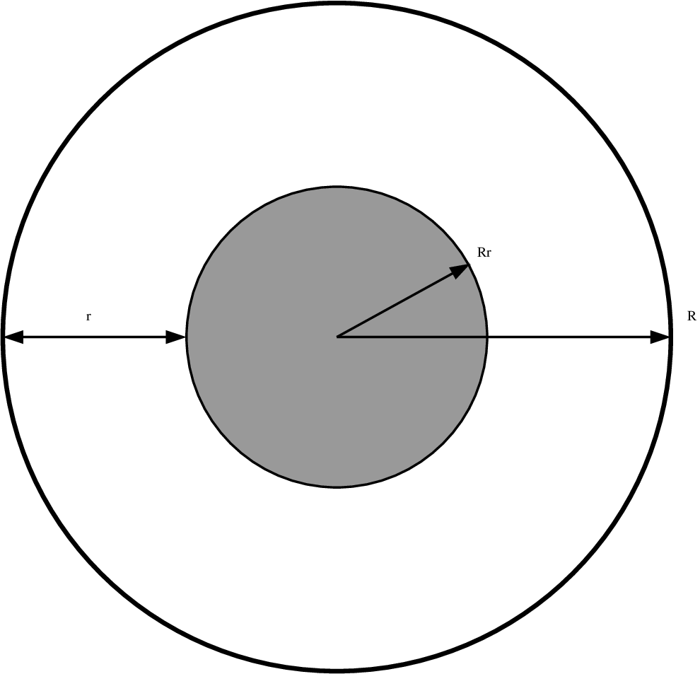
Refer to caption
(a)
Refer to caption
(b)
Figure 1. (a) Reference configuration for a circular film peeled off from a substrate. (b) Deformed configuration displaying the tension and the opening displacement exerted on the edge of the film.

We assume that the debonded region is parametrized on a growing annulus (Figure ??), whose width is given by a function ρ:[0,T]→[ρ0,R)\rho:[0,T]\to[\rho_{0},R), where R>ρ0>0R>\rho_{0}>0 are fixed. We assume

(1.1) ρ∈C0,1​([0,T],[ρ0,R)),ρ⁡(0)=ρ0​ and ​0≤ρ˙​(t)<1​ for a.e. ​t∈[0,T].\rho\in C^{0,1}([0,T];[\rho_{0},R)),\ \rho(0)=\rho_{0}\mbox{ and }0\leq\dot{\rho}(t)<1\mbox{ for a.e. }t\in[0,T].

For r<Rr<R, we define 𝒞r,R:={x∈ℝ2|r<|x|<R}\mathcal{C}_{r,R}:=\{x\in\mathbb{R}^{2}\,|\,r<|x|<R\} and

(1.2) 𝒪ρ:={(t,x)∈[0,+∞)×ℝ2| 0<t<T,x∈𝒞R−ρ⁡(t),R}.\mathcal{O}_{\rho}:=\{(t,x)\in[0,+\infty)\times\mathbb{R}^{2}\,|\,0<t<T,\ x\in\mathcal{C}_{R-\rho(t),R}\}.

At time tt, the debonded region is parametrized in the reference configuration on 𝒞R−ρ⁡(t),R\mathcal{C}_{R-\rho(t),R}.

Moreover, we fix a coefficient α≥0\alpha\geq 0 which governs a term related to the friction produced by air resistance on the vibrating film. Thus, for t∈[0,T]t\in[0,T] and x=(x1,x2)∈𝒞R−ρ⁡(t),Rx=(x_{1},x_{2})\in\mathcal{C}_{R-\rho(t),R}, the transverse component u⁡(t,x)u(t,x) of the displacement satisfies the following damped wave equation, complemented by initial and boundary conditions:

(1.3) {ut​t​(t,x)−Δx​u​(t,x)+α​ut​(t,x)=0t∈(0,T),R−ρ⁡(t)<|x|<R,u⁡(t,x)=w⁡(t)t∈(0,T),|x|=R,u⁡(t,x)=0t∈(0,T),|x|=R−ρ(t),u⁡(0,x)=u0​(x)R−ρ0<|x|<R,ut​(0,x)=u1​(x)R−ρ0<|x|<R.\begin{cases}u_{tt}(t,x)-\Delta_{x}u(t,x)+\alpha\,u_{t}(t,x)=0\qquad&t\in(0,T),\,R-\rho(t)<|x|<R,\\ u(t,x)=w(t)\qquad&t\in(0,T),\,|x|=R,\\ u(t,x)=0\qquad&t\in(0,T),\,|x|=R-\rho(t),\\ u(0,x)=u_{0}(x)\qquad&R-\rho_{0}<|x|<R,\\ u_{t}(0,x)=u_{1}(x)\qquad&R-\rho_{0}<|x|<R.\end{cases}

We look for solutions u∈W1,2​(𝒪ρ)u\in W^{1,2}(\mathcal{O}_{\rho}).

We remark that the boundary condition u⁡(t,x)=0u(t,x)=0 on {|x|=R−ρ(t)}\{|x|=R-\rho(t)\} models the fact that the film is still bonded to the substrate on that circle (and thus, on the whole disk {|x|≤R−ρ(t)}\{|x|\leq R-\rho(t)\}). On the other hand, the boundary condition u⁡(t,x)=w⁡(t)u(t,x)=w(t) on {|x|=R}\{|x|=R\} models the fact that the film is peeled off from the substrate through a tension exerted on its edge and an opening displacement w⁡(t)w(t), a given function of time corresponding to a time-dependent load. For simplicity we assume that no volume force is present. The initial conditions on the transverse displacement and its velocity are given by two functions of space u0​(x)u_{0}(x) and u1​(x)u_{1}(x), respectively, as usual for the wave equation. The requirement that ρ˙​(t)<1\dot{\rho}(t)<1 in () corresponds to the physical requirement that the debonding speed is subsonic, i.e., less than the wave speed.

We will seek for radial solutions of problem (), i.e., such that there exists U:[0,T]×(0,R)→ℝU:[0,T]\times(0,R)\to\mathbb{R} with u⁡(t,x)=U⁡(t,r)u(t,x)=U(t,r) for every t∈[0,T]t\in[0,T] and |x|=r|x|=r. Hence we define the following spaces:

Lrad2(𝒞r,R):={u∈L2(𝒞r,R)|∃u~:(r,R)→ℝ such that u(x)=u~(|x|) for a.e. x∈𝒞r,R},\displaystyle L^{2}_{\text{rad}}(\mathcal{C}_{r,R}):=\{u\in L^{2}(\mathcal{C}_{r,R})\,|\,\exists\,\tilde{u}:(r,R)\to\mathbb{R}\mbox{ such that }u(x)=\tilde{u}(|x|)\mbox{ for a.e. }x\in\mathcal{C}_{r,R}\},
Wrad1,2(𝒞r,R):={u∈W1,2(𝒞r,R)|∃u~:(r,R)→ℝ such that u(x)=u~(|x|) for a.e. x∈𝒞r,R},\displaystyle W^{1,2}_{\text{rad}}(\mathcal{C}_{r,R}):=\{u\in W^{1,2}(\mathcal{C}_{r,R})\,|\,\exists\,\tilde{u}:(r,R)\to\mathbb{R}\mbox{ such that }u(x)=\tilde{u}(|x|)\mbox{ for a.e. }x\in\mathcal{C}_{r,R}\},
Wrad1,2(B(0,R)):={u∈W1,2(B(0,R))|∃u~:(0,R)→ℝ such that u(x)=u~(|x|) for a.e. x∈B(0,R)}.\displaystyle W^{1,2}_{\text{rad}}(B(0,R)):=\{u\in W^{1,2}(B(0,R))\,|\,\exists\,\tilde{u}:(0,R)\to\mathbb{R}\mbox{ such that }u(x)=\tilde{u}(|x|)\mbox{ for a.e. }x\in B(0,R)\}.

We will assume that

(1.4) w∈W1,2​(0,T),u0∈Wrad1,2​(𝒞R−ρ0,R),u1∈Lrad2​(𝒞R−ρ0,R),w\in W^{1,2}(0,T),\quad u_{0}\in W^{1,2}_{\text{rad}}(\mathcal{C}_{R-\rho_{0},R}),\quad u_{1}\in L^{2}_{\text{rad}}(\mathcal{C}_{R-\rho_{0},R}),

with the compatibility conditions

(1.5) u0​(R)=w⁡(0),u0​(R−ρ0)=0.u_{0}(R)=w(0),\quad u_{0}(R-\rho_{0})=0.

We are now in a position to state the notion of solution to (). To this end, a standard argument allows one to make precise the initial condition on the velocity: given a solution u∈W1,2​(𝒪ρ)u\in W^{1,2}(\mathcal{O}_{\rho}), we consider the restriction of u⁡(t)u(t) to 𝒞ρ0,R\mathcal{C}_{\rho_{0},R}; since ut,ux∈L2​((0,T),L2​(𝒞ρ0,R))u_{t},u_{x}\in L^{2}((0,T);L^{2}(\mathcal{C}_{\rho_{0},R})), then ut​t=Δx​u​(t,x)−α​ut​(t,x)∈L2​((0,T),W−1,2​(𝒞ρ0,R))u_{tt}=\Delta_{x}u(t,x)-\alpha\,u_{t}(t,x)\in L^{2}((0,T);W^{-1,2}(\mathcal{C}_{\rho_{0},R})), hence ut∈W1,2​((0,T),W−1,2​(𝒞ρ0,R))⊂C0​([0,T],W−1,2​(𝒞ρ0,R))u_{t}\in W^{1,2}((0,T);W^{-1,2}(\mathcal{C}_{\rho_{0},R}))\subset C^{0}([0,T];W^{-1,2}(\mathcal{C}_{\rho_{0},R})).

Definition 1.1.

We say that a function u∈W1,2​(𝒪ρ)u\in W^{1,2}(\mathcal{O}_{\rho}) is a solution of () if

  1. (1)

    ut​t​(t,x)−Δx​u​(t,x)+α​ut​(t,x)=0u_{tt}(t,x)-\Delta_{x}u(t,x)+\alpha\,u_{t}(t,x)=0 holds in the sense of distributions in 𝒪ρ\mathcal{O}_{\rho},

  2. (2)

    the boundary conditions are satisfied in the trace sense,

  3. (3)

    the initial conditions are satisfied in the sense of L2​(𝒞R−ρ0,R)L^{2}(\mathcal{C}_{R-\rho_{0},R}) and W−1,2​(𝒞R−ρ0,R)W^{-1,2}(\mathcal{C}_{R-\rho_{0},R}) respectively.

We say that uu is a radial solution if in addition u⁡(t,⋅)∈Wrad1,2​(𝒞R−ρ⁡(t),R)u(t,\cdot)\in W^{1,2}_{\text{rad}}(\mathcal{C}_{R-\rho(t),R}) for a.e. t∈[0,T]t\in[0,T].

It will be more convenient for our analysis to introduce the following transformation:

(1.6) v⁡(t,r)=u⁡(t,x) for ​t∈(0,T),|x|=R−r,v(t,r)=u(t,x)\quad\mbox{ for }t\in(0,T),\,|x|=R-r,

where the initial conditions are defined in an analogous way:

(1.7) v0​(r)=u0​(x),v1​(r)=u1​(x) with ​|x|=R−r.v_{0}(r)=u_{0}(x),\quad v_{1}(r)=u_{1}(x)\quad\mbox{ with }|x|=R-r.

Then, passing to polar coordinates, we get that uu solves () if and only if vv solves the following system:

(1.8) {vt​t​(t,r)−vr​r​(t,r)+1R−r​vr​(t,r)+α​vt​(t,r)=0t∈(0,T), 0<r<ρ(t),v⁡(t,0)=w⁡(t)t∈(0,T),v⁡(t,ρ⁡(t))=0t∈(0,T),v⁡(0,r)=v0​(r)0<r<ρ0,vt​(0,r)=v1​(r)0<r<ρ0.\begin{cases}v_{tt}(t,r)-v_{rr}(t,r)+\frac{1}{R-r}\,v_{r}(t,r)+\alpha\,v_{t}(t,r)=0\qquad&t\in(0,T),\,0<r<\rho(t),\\ v(t,0)=w(t)\qquad&t\in(0,T),\\ v(t,\rho(t))=0\qquad&t\in(0,T),\\ v(0,r)=v_{0}(r)\qquad&0<r<\rho_{0},\\ v_{t}(0,r)=v_{1}(r)\qquad&0<r<\rho_{0}.\end{cases}

We notice that if w,u0w,u_{0} and u1u_{1} satisfy () and (), then

(1.9) w∈W1,2​(0,T),v0∈W1,2​(0,ρ0),v1∈L2​(0,ρ0),w\in W^{1,2}(0,T),\quad v_{0}\in W^{1,2}(0,\rho_{0}),\quad v_{1}\in L^{2}(0,\rho_{0}),

and the following compatibility conditions hold:

(1.10) v0​(0)=w⁡(0),v0​(ρ0)=0.v_{0}(0)=w(0),\quad v_{0}(\rho_{0})=0.

1.1. Equivalent reformulation

We now introduce the function

(1.11) h⁡(t,r):=(R−r)12​eα2​t​v​(t,r)t∈(0,T), 0<r<R.h(t,r):=(R-r)^{\frac{1}{2}}\,e^{\frac{\alpha}{2}t}\,v(t,r)\qquad t\in(0,T),\,0<r<R.

Simple computations give the following relations:

vt​(t,r)=(R−r)−12​e−α2​t​(ht​(t,r)−α2​h​(t,r)),vr​(t,r)=(R−r)−12​e−α2​t​(hr​(t,r)+12​(R−r)−1​h​(t,r)),vt​t​(t,r)=(R−r)−12​e−α2​t​(ht​t​(t,r)−α​ht​(t,r)+α24​h​(t,r)),vr​r​(t,r)=(R−r)−12​e−α2​t​(hr​r​(t,r)+(R−r)−1​hr​(t,r)+34​(R−r)−2​h​(t,r)).\begin{split}v_{t}(t,r)&=(R-r)^{-\frac{1}{2}}\,e^{-\frac{\alpha}{2}t}\left(h_{t}(t,r)-\frac{\alpha}{2}\,h(t,r)\right),\\ v_{r}(t,r)&=(R-r)^{-\frac{1}{2}}\,e^{-\frac{\alpha}{2}t}\left(h_{r}(t,r)+\frac{1}{2}(R-r)^{-1}\,h(t,r)\right),\\ v_{tt}(t,r)&=(R-r)^{-\frac{1}{2}}\,e^{-\frac{\alpha}{2}t}\left(h_{tt}(t,r)-\alpha\,h_{t}(t,r)+\frac{\alpha^{2}}{4}\,h(t,r)\right),\\ v_{rr}(t,r)&=(R-r)^{-\frac{1}{2}}\,e^{-\frac{\alpha}{2}t}\left(h_{rr}(t,r)+(R-r)^{-1}\,h_{r}(t,r)+\frac{3}{4}(R-r)^{-2}\,h(t,r)\right).\end{split}

Then from () we get the auxiliary problem

(1.12) {ht​t​(t,r)−hr​r​(t,r)−14​(α2+1(R−r)2)​h​(t,r)=0t∈(0,T), 0<r<ρ(t),h⁡(t,0)=z⁡(t)t∈(0,T),h⁡(t,ρ⁡(t))=0t∈(0,T),h⁡(0,r)=h0​(r)0<r<ρ0,ht​(0,r)=h1​(r)0<r<ρ0,\begin{cases}h_{tt}(t,r)-h_{rr}(t,r)-\frac{1}{4}\left(\alpha^{2}+\frac{1}{\left(R-r\right)^{2}}\right)\,h(t,r)=0\qquad&t\in(0,T),\,0<r<\rho(t),\\ h(t,0)=z(t)\qquad&t\in(0,T),\\ h(t,\rho(t))=0\qquad&t\in(0,T),\\ h(0,r)=h_{0}(r)\qquad&0<r<\rho_{0},\\ h_{t}(0,r)=h_{1}(r)\qquad&0<r<\rho_{0},\end{cases}

where the boundary conditions and the initial data are given by

(1.13) {z⁡(t):=R12​eα​t2​w​(t),h0​(r):=(R−r)12​v0​(r),h1​(r):=(R−r)12​(v1​(r)+α2​v0​(r)).\begin{cases}z(t):=R^{\frac{1}{2}}\,e^{\alpha\frac{t}{2}}\,w(t),\\ h_{0}(r):=(R-r)^{\frac{1}{2}}\,v_{0}(r),\\ h_{1}(r):=(R-r)^{\frac{1}{2}}\,\left(v_{1}(r)+\frac{\alpha}{2}v_{0}(r)\right).\end{cases}

We mention that if w,v0w,v_{0} and v1v_{1} satisfy () and (), then z,h0z,h_{0} and h1h_{1} satisfy

(1.14) z∈W1,2​(0,T),h0∈W1,2​(0,ρ0),h1∈L2​(0,ρ0),z\in W^{1,2}(0,T),\quad h_{0}\in W^{1,2}(0,\rho_{0}),\quad h_{1}\in L^{2}(0,\rho_{0}),

with the compatibility conditions

(1.15) h0​(0)=z⁡(0),h0​(ρ0)=0.h_{0}(0)=z(0),\quad h_{0}(\rho_{0})=0.

Moreover uu is a solution of problem () if and only if hh is a solution of ().

In [30] the authors studied the equations

ht​t−hx​x+α​ht=0andht​t−hx​x−α24​h=0.h_{tt}-h_{xx}+\alpha\,h_{t}=0\quad\text{and}\quad h_{tt}-h_{xx}-\frac{\alpha^{2}}{4}\,h=0.

When dealing with (), which features a nonconstant kernel multiplying a first derivative, we will follow an approach similar to the one of [30], based on representation formulas for the damped one-dimensional wave equation. Thus, as in [11] we introduce two functions defined for t∈[0,T]t\in[0,T],

ϕ⁡(t):=t−ρ⁡(t)​ and ​ψ​(t):=t+ρ⁡(t).\phi(t):=t-\rho(t)\mbox{ and }\psi(t):=t+\rho(t).

Since ψ\psi is strictly increasing, we can then define

ω:=[0,T+ρ⁡(T)]→[−ρ0,T−ρ⁡(T)],ω⁡(t):={ϕ∘ψ(−1)​(t)if​t≥ρ0,−ρ0if​t<ρ0,\omega:=[0,T{+}\rho(T)]\to[-\rho_{0},T{-}\rho(T)],\quad\omega(t):=\begin{cases}\phi\circ\psi^{(-1)}(t)&\ \text{if}\ t\geq\rho_{0},\\ -\rho_{0}&\ \text{if}\ t<\rho_{0},\end{cases}

and we notice that ω\omega is a Lipschitz function whose derivative satisfies for a.e. t∈[0,T]t\in[0,T]

0≤ω˙​(t)=1−ρ˙​(ψ(−1)​(t))1+ρ˙​(ψ(−1)​(t))≤1.0\leq\dot{\omega}(t)=\frac{1-\dot{\rho}(\psi^{(-1)}(t))}{1+\dot{\rho}(\psi^{(-1)}(t))}\leq 1.

We introduce the sets

(1.16) Ω:={(t,r)∈(0,T)×(0,R)| 0<r<ρ⁡(t)},\displaystyle\Omega:=\{(t,r)\in(0,T)\times(0,R)\,|\,0<r<\rho(t)\},
Ω1′:={(t,r)∈Ω|t≤r​ and ​t+r≤ρ0},\displaystyle\Omega^{\prime}_{1}:=\{(t,r)\in\Omega\,|\,t\leq r\mbox{ and }t+r\leq\rho_{0}\},
Ω2′:={(t,r)∈Ω|t>r​ and ​t+r<ρ0},\displaystyle\Omega^{\prime}_{2}:=\{(t,r)\in\Omega\,|\,t>r\mbox{ and }t+r<\rho_{0}\},
Ω3′:={(t,r)∈Ω|t<r​ and ​t+r>ρ0},\displaystyle\Omega^{\prime}_{3}:=\{(t,r)\in\Omega\,|\,t<r\mbox{ and }t+r>\rho_{0}\},
Ω′:=Ω1′∪Ω2′∪Ω3′.\displaystyle\Omega^{\prime}:=\Omega^{\prime}_{1}\cup\Omega^{\prime}_{2}\cup\Omega^{\prime}_{3}.

Moreover we define the dependence cone of the point (t,r)(t,r), given by

Refer to caption
(a)
Refer to caption
(b)
Refer to caption
(c)
Figure 2. Sets appearing in formula () in the three cases (t,r)∈Ω1′(t,r)\in\Omega^{\prime}_{1} (a), (t,r)∈Ω2′(t,r)\in\Omega^{\prime}_{2} (b), (t,r)∈Ω3′(t,r)\in\Omega^{\prime}_{3} (c). For convenience the tt-axis is vertical. In each case the region in dark gray is the set P⁡(t,r)P(t,r), while the dependence cone C⁡(t,r)C(t,r) is the union of the regions in dark and light gray.
(1.17) C⁡(t,r):={(τ,σ)∈Ω| 0≤τ≤t​ and ​r−t+τ≤σ≤r+t−τ}.C(t,r):=\{(\tau,\sigma)\in\Omega\,|\,0\leq\tau\leq t\mbox{ and }r-t+\tau\leq\sigma\leq r+t-\tau\}.

It will turn useful to define the set P⁡(t,r)P(t,r) as

(1.18) P⁡(t,r):={C⁡(t,r) if ​t<r​ and ​t+r<ρ0,C⁡(t,r)∖C⁡(t−r,0) if ​t>r​ and ​t+r<ρ0,C⁡(t,r)∖C⁡(ψ−1​(t+r),ρ⁡(ψ−1​(t+r))) if ​t<r​ and ​t+r>ρ0.P(t,r):=\begin{cases}C(t,r)&\mbox{ if }t<r\mbox{ and }t+r<\rho_{0},\\ C(t,r)\setminus C(t-r,0)&\mbox{ if }t>r\mbox{ and }t+r<\rho_{0},\\ C(t,r)\setminus C(\psi^{-1}(t{+}r),\rho(\psi^{-1}(t{+}r)))&\mbox{ if }t<r\mbox{ and }t+r>\rho_{0}.\end{cases}

See Figure ??.

Consider now the undamped wave equation in the time-dependent interval (0,ρ⁡(t))(0,\rho(t)), complemented with initial and boundary conditions as in (),

(1.19) {ℌt​t​(t,r)−ℌr​r​(t,r)=0t∈(0,T), 0<r<ρ(t),ℌ⁡(t,0)=z⁡(t)t∈(0,T),ℌ⁡(t,ρ⁡(t))=0t∈(0,T),ℌ⁡(0,r)=h0​(r)0<r<ρ0,ℌt​(0,r)=h1​(r)0<r<ρ0.\begin{cases}\mathfrak{H}_{tt}(t,r)-\mathfrak{H}_{rr}(t,r)=0\qquad&t\in(0,T),\,0<r<\rho(t),\\ \mathfrak{H}(t,0)=z(t)\qquad&t\in(0,T),\\ \mathfrak{H}(t,\rho(t))=0\qquad&t\in(0,T),\\ \mathfrak{H}(0,r)=h_{0}(r)\qquad&0<r<\rho_{0},\\ \mathfrak{H}_{t}(0,r)=h_{1}(r)\qquad&0<r<\rho_{0}.\end{cases}

In [11] it has been shown that this problem has a unique solution ℌ\mathfrak{H}, which satisfies the following d’Alembert formula in Ω′\Omega^{\prime}:

(1.20) ℌ⁡(t,r)={12​h0​(r−t)+12​h0​(r+t)+12​∫r−tr+th1​(s)​𝑑s if ​(t,r)∈Ω1′,z⁡(t−r)−12​h0​(t−r)+12​h0​(r+t)+12​∫t−rt+rh1​(s)​𝑑s if ​(t,r)∈Ω2′,12​h0​(r−t)−12​h0​(−ω⁡(r+t))+12​∫r−t−ω⁡(r+t)h1​(s)​𝑑s if ​(t,r)∈Ω3′.\mathfrak{H}(t,r)=\begin{cases}\frac{1}{2}h_{0}(r{-}t)+\frac{1}{2}h_{0}(r{+}t)+\frac{1}{2}\int_{r-t}^{r+t}h_{1}(s)\,ds&\mbox{ if }(t,r)\in\Omega^{\prime}_{1},\\ z(t{-}r)-\frac{1}{2}h_{0}(t{-}r)+\frac{1}{2}h_{0}(r{+}t)+\frac{1}{2}\int_{t-r}^{t+r}h_{1}(s)\,ds&\mbox{ if }(t,r)\in\Omega^{\prime}_{2},\\ \frac{1}{2}h_{0}(r{-}t)-\frac{1}{2}h_{0}(-\omega(r{+}t))+\frac{1}{2}\int_{r-t}^{-\omega(r+t)}h_{1}(s)\,ds&\mbox{ if }(t,r)\in\Omega^{\prime}_{3}.\end{cases}

Indeed, according to the principle of causality, ℌ\mathfrak{H} depends on the data interior to the dependence cone.

By a standard computation (which we detail for the reader’s convenience), we may derive a law holding for any solution of problem ().

Proposition 1.2.

A function h∈W1,2​(Ω′)h\in W^{1,2}(\Omega^{\prime}) is a solution of problem () in Ω′\Omega^{\prime} if and only if

(1.21) h⁡(t,r)=ℌ⁡(t,r)+12​∬P⁡(t,r)14​(α2+1(R−σ)2)​h​(τ,σ)​𝑑σ​𝑑τ for a.e.​(t,r)∈Ω′,h(t,r)=\mathfrak{H}(t,r)+\frac{1}{2}\iint_{P(t,r)}\frac{1}{4}\left(\alpha^{2}+\frac{1}{\left(R-\sigma\right)^{2}}\right)\,h(\tau,\sigma)\,d\sigma\,d\tau\quad\mbox{ for a.e.}\,(t,r)\in\Omega^{\prime},

where P⁡(t,r)P(t,r) and ℌ\mathfrak{H} are given by () and (), respectively.

Proof.

Let h∈W1,2​(Ω′)h\in W^{1,2}(\Omega^{\prime}) be a solution of problem () and consider the following change of variables,

(1.22) {ξ=t−r,η=t+r.\begin{cases}\xi=t-r,\\ \eta=t+r.\end{cases}

We remark en passant that the line t=0t=0 corresponds to ξ+η=0\xi+\eta=0. Then the function h~​(ξ,η):=h​(ξ+η2,η−ξ2)\tilde{h}(\xi,\eta):=h\left(\frac{\xi+\eta}{2},\frac{\eta-\xi}{2}\right) satisfies

(1.23) ∂ξ,ηh~=116​(α2+1(R−η−ξ2)2)​h~\partial_{\xi,\eta}\,\tilde{h}=\frac{1}{16}\left(\alpha^{2}+\frac{1}{\left(R-\frac{\eta-\xi}{2}\right)^{2}}\right)\,\tilde{h}

in the sense of distributions in Λ′\Lambda^{\prime}, where Λ′\Lambda^{\prime} is the image of Ω′\Omega^{\prime} through the affine transformation (). Let us denote by Λi′\Lambda^{\prime}_{i} the image of Ωi′\Omega^{\prime}_{i} through the change of coordinates (i=1,2,3i=1,2,3). Now define the right-hand side of () by H~\widetilde{H} and denote by C~​(ξ,η)\widetilde{C}(\xi,\eta) and P~​(ξ,η)\widetilde{P}(\xi,\eta) the sets given by () and (), respectively, in terms of the new coordinates. We fix a point (t¯,r¯)∈Ω′(\overline{t},\overline{r})\in\Omega^{\prime}, corresponding to (ξ¯,η¯)∈Λ′(\overline{\xi},\overline{\eta})\in\Lambda^{\prime}, and distinguish the three cases where such point lies in Λ1′\Lambda_{1}^{\prime}, Λ2′\Lambda_{2}^{\prime}, or Λ3′\Lambda_{3}^{\prime}.

(1) Case (ξ¯,η¯)∈Λ1′(\overline{\xi},\overline{\eta})\in\Lambda_{1}^{\prime}: Observe that in this case one has ξ¯≤0\overline{\xi}\leq 0 and P~​(ξ¯,η¯)=C~​(ξ¯,η¯)\widetilde{P}(\overline{\xi},\overline{\eta})=\widetilde{C}(\overline{\xi},\overline{\eta}) is defined by the conditions −η¯≤ξ≤ξ¯-\overline{\eta}\leq\xi\leq\overline{\xi} and |ξ|≤η≤η¯|\xi|\leq\eta\leq\overline{\eta}, where we took into account that ξ≤0\xi\leq 0 on the given domain (see Figure ??). By double integration one gets:

h~​(ξ¯,η¯)=h~​(−η¯,η¯)+∫−η¯ξ¯h~ξ​(ξ,|ξ|)​𝑑ξ+∬P~​(ξ¯,η¯)H~​(ξ,η)​𝑑ξ​𝑑η.\tilde{h}(\overline{\xi},\overline{\eta})=\tilde{h}(-\overline{\eta},\overline{\eta})+\int_{-\overline{\eta}}^{\overline{\xi}}\tilde{h}_{\xi}(\xi,|\xi|)\,d\xi+\iint_{\widetilde{P}(\overline{\xi},\overline{\eta})}\widetilde{H}(\xi,\eta)\,d\xi\,d\eta.

Then, by a change of variables in the last integral from the domain of integration P~​(ξ¯,η¯)\widetilde{P}(\overline{\xi},\overline{\eta}) to P⁡(t¯,r¯)P(\overline{t},\overline{r}), by observing that h~​(−η¯,η¯)=h0​(r¯+t¯)\tilde{h}(-\overline{\eta},\overline{\eta})=h_{0}(\overline{r}+\overline{t}) and by computing

∫−η¯ξ¯h~ξ​(ξ,|ξ|)​𝑑ξ\displaystyle\int_{-\overline{\eta}}^{\overline{\xi}}\tilde{h}_{\xi}(\xi,|\xi|)\,d\xi =−12∫r¯+t¯r¯−t¯(ht(0,r)−hr(0,r))dr\displaystyle=-\frac{1}{2}\int_{\overline{r}+\overline{t}}^{\overline{r}-\overline{t}}(h_{t}(0,r)-h_{r}(0,r))\,dr
=12​h0​(r¯−t¯)−12​h0​(r¯+t¯)+12​∫r¯−t¯r¯+t¯h1​(s)​𝑑s,\displaystyle=\frac{1}{2}h_{0}(\overline{r}-\overline{t})-\frac{1}{2}h_{0}(\overline{r}+\overline{t})+\frac{1}{2}\int_{\overline{r}-\overline{t}}^{\overline{r}+\overline{t}}h_{1}(s)\,ds,

one obtains that () holds in Ω1′\Omega^{\prime}_{1} (see also Figure ??).

Refer to caption
Figure 3. Some points appearing in the proof of Proposition ??, represented in the (t,r)(t,r)-plane (with rr on the horizontal axis) and marked using the (ξ,η)(\xi,\eta)-coordinates. The bold curve is the graph of t↦ρ⁡(t)t\mapsto\rho(t). In the picture we consider three points (ξ¯,η¯)∈Λ1′(\overline{\xi},\overline{\eta})\in\Lambda^{\prime}_{1}, (ξ¯,η¯)∈Λ2′(\underline{\xi},\overline{\eta})\in\Lambda^{\prime}_{2}, (ξ¯,η¯)∈Λ3′(\overline{\xi},\underline{\eta})\in\Lambda^{\prime}_{3}; notice that ξ¯<0<ξ¯\overline{\xi}<0<\underline{\xi}. The other points, lying on the characteristic lines, are the boundary points in the double integrations in the proof. Here we use the shorthand notation ω¯:=ω⁡(η¯)\underline{\omega}:=\omega(\underline{\eta}).

(2) Case (ξ¯,η¯)∈Λ2′(\overline{\xi},\overline{\eta})\in\Lambda_{2}^{\prime}: Observe that in this case P~​(ξ¯,η¯)\widetilde{P}(\overline{\xi},\overline{\eta}) is defined by the conditions ξ¯≤η≤η¯\overline{\xi}\leq\eta\leq\overline{\eta} and −η≤ξ≤ξ¯-\eta\leq\xi\leq\overline{\xi} (see Figure ??). By double integration one gets:

h~​(ξ¯,η¯)=h~​(ξ¯,ξ¯)+∫ξ¯η¯h~η​(−η,η)​𝑑η+∬P~​(ξ¯,η¯)H~​(ξ,η)​𝑑ξ​𝑑η.\tilde{h}(\overline{\xi},\overline{\eta})=\tilde{h}(\overline{\xi},\overline{\xi})+\int_{\overline{\xi}}^{\overline{\eta}}\tilde{h}_{\eta}(-\eta,\eta)\,d\eta+\iint_{\widetilde{P}(\overline{\xi},\overline{\eta})}\widetilde{H}(\xi,\eta)\,d\xi\,d\eta.

Then, by changing the variables in the last integral from the domain of integration P~​(ξ¯,η¯)\widetilde{P}(\overline{\xi},\overline{\eta}) back to P⁡(t¯,r¯)P(\overline{t},\overline{r}), by observing that h~​(ξ¯,ξ¯)=z​(t¯−r¯)\tilde{h}(\overline{\xi},\overline{\xi})=z(\overline{t}-\overline{r}) and h~​(−η¯,η¯)=h0​(t¯+r¯)\tilde{h}(-\overline{\eta},\overline{\eta})=h_{0}(\overline{t}+\overline{r}) and by computing

∫ξ¯η¯h~η​(−η,η)​𝑑η\displaystyle\int_{\overline{\xi}}^{\overline{\eta}}\tilde{h}_{\eta}(-\eta,\eta)\,d\eta =12​∫t¯−r¯t¯+r¯(ht​(0,r)+hr​(0,r))​𝑑r\displaystyle=\frac{1}{2}\int_{\overline{t}-\overline{r}}^{\overline{t}+\overline{r}}(h_{t}(0,r)+h_{r}(0,r))\,dr
=−12​h0​(t¯−r¯)+12​h0​(r¯+t¯)+12​∫t¯−r¯r¯+t¯h1​(s)​𝑑s,\displaystyle=-\frac{1}{2}h_{0}(\overline{t}-\overline{r})+\frac{1}{2}h_{0}(\overline{r}+\overline{t})+\frac{1}{2}\int_{\overline{t}-\overline{r}}^{\overline{r}+\overline{t}}h_{1}(s)\,ds,

one obtains that () holds in Ω2′\Omega^{\prime}_{2} (see also Figure ??).

(3) Case (ξ¯,η¯)∈Λ3′(\overline{\xi},\overline{\eta})\in\Lambda_{3}^{\prime}: Observe that in this case one has ξ¯<0\overline{\xi}<0 and P~​(ξ¯,η¯)\widetilde{P}(\overline{\xi},\overline{\eta}) is defined by the conditions ω⁡(η¯)≤ξ≤ξ¯\omega(\overline{\eta})\leq\xi\leq\overline{\xi} and |ξ|≤η≤η¯|\xi|\leq\eta\leq\overline{\eta}, where we took into account that ξ<0\xi<0 on the given domain (see Figure ??). By double integration one gets:

h~​(ξ¯,η¯)=h~​(ω⁡(η¯),η¯)+∫ω⁡(η¯)ξ¯h~ξ​(ξ,|ξ|)​𝑑ξ+∬P~​(ξ¯,η¯)H~​(ξ,η)​𝑑ξ​𝑑η.\tilde{h}(\overline{\xi},\overline{\eta})=\tilde{h}(\omega(\overline{\eta}),\overline{\eta})+\int_{\omega(\overline{\eta})}^{\overline{\xi}}\tilde{h}_{\xi}(\xi,|\xi|)\,d\xi+\iint_{\widetilde{P}(\overline{\xi},\overline{\eta})}\widetilde{H}(\xi,\eta)\,d\xi\,d\eta.

Then, by a change of variables in the last integral from P~​(ξ¯,η¯)\widetilde{P}(\overline{\xi},\overline{\eta}) to P⁡(t¯,r¯)P(\overline{t},\overline{r}), by observing that h~​(ω​(η¯),η¯)=0\tilde{h}(\omega(\overline{\eta}),\overline{\eta})=0 and by computing

∫ω⁡(η¯)ξ¯h~ξ​(ξ,|ξ|)​𝑑ξ\displaystyle\int_{\omega(\overline{\eta})}^{\overline{\xi}}\tilde{h}_{\xi}(\xi,|\xi|)\,d\xi =−12∫−ω⁡(r¯+t¯)r¯−t¯(ht(0,r)−hr(0,r))(r)dr\displaystyle=-\frac{1}{2}\int_{-\omega(\overline{r}+\overline{t})}^{\overline{r}-\overline{t}}(h_{t}(0,r)-h_{r}(0,r))(r)\,dr
=12​h0​(r¯−t¯)−12​h0​(−ω⁡(r¯+t¯))+12​∫r¯−t¯−ω⁡(r¯+t¯)h1​(s)​𝑑s,\displaystyle=\frac{1}{2}h_{0}(\overline{r}-\overline{t})-\frac{1}{2}h_{0}(-\omega(\overline{r}+\overline{t}))+\frac{1}{2}\int_{\overline{r}-\overline{t}}^{-\omega(\overline{r}+\overline{t})}h_{1}(s)\,ds,

one obtains that () holds in Ω3′\Omega^{\prime}_{3} (see also Figure ??).

Finally, to prove the converse implication it is sufficient to show that J⁡(ξ¯,η¯):=∬P~​(ξ¯,η¯)H~​(ξ,η)​𝑑ξ​𝑑ηJ(\overline{\xi},\overline{\eta}):=\iint_{\widetilde{P}(\overline{\xi},\overline{\eta})}\widetilde{H}(\xi,\eta)\,d\xi\,d\eta solves ∂ξ,η2J⁡(ξ¯,η¯)=H~​(ξ¯,η¯)\partial^{2}_{\xi,\eta}J(\overline{\xi},\overline{\eta})=\widetilde{H}(\overline{\xi},\overline{\eta}). We detail the computation only in case (3), the others being similar. In this case,

J(ξ¯,η¯)=∫ω⁡(η¯)ξ¯∫|ξ|η¯H~​(ξ,η)​dη⏟=:j⁡(ξ,η¯)dξ.J(\overline{\xi},\overline{\eta})=\int_{\omega(\overline{\eta})}^{\overline{\xi}}\underbrace{\int_{|\xi|}^{\overline{\eta}}\widetilde{H}(\xi,\eta)\,d\eta}_{=:j(\xi,\overline{\eta})}\,d\xi.

We then have ∂ηJ⁡(ξ¯,η¯)=−j⁡(ω⁡(η¯),η¯)​ω˙​(η¯)+∫ω⁡(η¯)ξ¯H~​(ξ,η¯)​𝑑ξ\partial_{\eta}J(\overline{\xi},\overline{\eta})=-j(\omega(\overline{\eta}),\overline{\eta})\,\dot{\omega}(\overline{\eta})+\int_{\omega(\overline{\eta})}^{\overline{\xi}}\widetilde{H}(\xi,\overline{\eta})\,d\xi. By deriving with respect to ξ¯\overline{\xi} the conclusion follows immediately. ∎

Below we shall use the following formula for the solutions of problem ().

Remark 1.3.

Let vv be a solution of problem (). Let 𝔙\mathfrak{V} be the solution of the pure wave equation given by () replacing the boundary data h0h_{0}, h1h_{1}, and zz by v0v_{0}, v1v_{1}, and ww, respectively. Then the very same argument of Proposition ?? shows that

(1.24) v⁡(t,r)=𝔙⁡(t,r)+12​∬P⁡(t,r)(−vr​(τ,σ)(R−r)−α​vt​(τ,σ))​𝑑σ​𝑑τ for a.e.​(t,r)∈Ω′.v(t,r)=\mathfrak{V}(t,r)+\frac{1}{2}\iint_{P(t,r)}\left(-\frac{v_{r}(\tau,\sigma)}{\left(R{-}r\right)}-\alpha\,v_{t}(\tau,\sigma)\right)\,d\sigma\,d\tau\quad\mbox{ for a.e.}\,(t,r)\in\Omega^{\prime}.

We summarize the regularity of the terms appearing in () in the following lemma. (For a detailed proof we refer to [30, Lemmas 1.10 and 1.11].)

Lemma 1.4.

The following hold true.

  1. (i)

    Let ℌ\mathfrak{H} be defined as in (). Then ℌ∈C0(Ω¯)′∩W1,2(Ω′)\mathfrak{H}\in C^{0}(\overline{\Omega}{}^{\prime})\cap W^{1,2}(\Omega^{\prime}). Moreover, setting ℌ≡0\mathfrak{H}\equiv 0 outside Ω¯\overline{\Omega},

    ℌ∈C0​([0,T],W1,2​(0,R))∩C1​([0,T],L2​(0,R)).\mathfrak{H}\in C^{0}([0,T];W^{1,2}(0,R))\cap C^{1}([0,T];L^{2}(0,R)).
  2. (ii)

    Let H∈L2​(Ω′)H\in L^{2}(\Omega^{\prime}) and for every (t,r)∈Ω′(t,r)\in\Omega^{\prime} define

    (1.25) Φ⁡[H]​(t,r):=∬P⁡(t,r)H⁡(τ,σ)​𝑑τ​𝑑σ.\Phi[H](t,r):=\iint_{P(t,r)}H(\tau,\sigma)\,d\tau d\sigma.

    Then Φ[H]∈C0(Ω¯)′∩W1,2(Ω′)\Phi[H]\in C^{0}(\overline{\Omega}{}^{\prime})\cap W^{1,2}(\Omega^{\prime}). Moreover, setting Φ⁡[H]≡0\Phi[H]\equiv 0 outside Ω¯\overline{\Omega},

    Φ⁡[H]∈C0​([0,T],W1,2​(0,R))∩C1​([0,T],L2​(0,R)).\Phi[H]\in C^{0}([0,T];W^{1,2}(0,R))\cap C^{1}([0,T];L^{2}(0,R)).

1.2. Existence of solutions for prescribed debonding front

In order to obtain existence and uniqueness of a solution to problem (), we first seek a solution in a small time interval [0,T~]⊂[0,T][0,\widetilde{T}]\subset[0,T]; afterwards we shall extend the solution to [0,T][0,T]. As a consequence, we have existence and uniqueness of a radial solution to problem (); moreover, if ρ\rho is sufficiently regular, the results in Appendix ?? show that such radial function is the unique solution to problem () in the sense of Definition ??. The solution to () is found as a fixed point of a certain linear operator. More precisely, let

𝒴:={h∈C0(Ω¯)′|h satisfies the initial and boundary conditions in ()}\mathcal{Y}:=\{h\in C^{0}(\overline{\Omega}{}^{\prime})\,|\,h\mbox{ satisfies the initial and boundary conditions in }\eqref{princeqh}\}

and consider

ℒ:𝒴→C0(Ω¯)′,h↦ℒ[h]\mathcal{L}:\,\mathcal{Y}\to C^{0}(\overline{\Omega}{}^{\prime}),\,h\mapsto\mathcal{L}[h]

defined by

(1.26) ℒ⁡[h]​(t,r):=ℌ⁡(t,r)+12​∬P⁡(t,r)14​(α2+1(R−σ)2)​h​(τ,σ)​𝑑σ​𝑑τ for a.e.​(t,r)∈Ω′.\mathcal{L}[h](t,r):=\mathfrak{H}(t,r)+\frac{1}{2}\iint_{P(t,r)}\frac{1}{4}\left(\alpha^{2}+\frac{1}{\left(R{-}\sigma\right)^{2}}\right)\,h(\tau,\sigma)\,d\sigma\,d\tau\quad\mbox{ for a.e.}\,(t,r)\in\Omega^{\prime}.

Then we have the following result, the proof of which is based on [30, Proposition 1.13]; we detail the proof in order to show how the kernel 14​(α2+1(R−σ)2)\frac{1}{4}\left(\alpha^{2}+\frac{1}{\left(R{-}\sigma\right)^{2}}\right) affects the constant in (). We employ the following notation:

ΩS:={(t,r)∈Ω|t<S}\Omega_{S}:=\{(t,r)\in\Omega\,|\,t<S\}

for S∈(0,T)S\in(0,T).

Proposition 1.5.

Let ρ~:=min⁡{ρ02,R−ρ02}\tilde{\rho}:=\min\left\{\frac{\rho_{0}}{2},\frac{R{-}\rho_{0}}{2}\right\}. Let T~∈(0,ρ~)\widetilde{T}\in(0,\tilde{\rho}) satisfy

(1.27) ρ0​T~4​(α2+4(R−ρ0)2)<1.\frac{\rho_{0}\widetilde{T}}{4}\left(\alpha^{2}+\frac{4}{\left(R{-}\rho_{0}\right)^{2}}\right)<1.

Then operator ℒ\mathcal{L} defined by () is a contraction from 𝒴∩C0​(Ω¯T~)\mathcal{Y}\cap C^{0}(\overline{\Omega}_{\widetilde{T}}) into C0​(Ω¯T~)C^{0}(\overline{\Omega}_{\widetilde{T}}).

Proof.

By Lemma ?? the operator ℒ\mathcal{L} maps 𝒴∩C0​(Ω¯T~)\mathcal{Y}\cap C^{0}(\overline{\Omega}_{\widetilde{T}}) into itself. Now let h(1),h(2)∈𝒴∩C0​(Ω¯T~)h^{(1)},h^{(2)}\in\mathcal{Y}\cap C^{0}(\overline{\Omega}_{\widetilde{T}}) and let (t,r)∈Ω¯T~(t,r)\in\overline{\Omega}_{\widetilde{T}}. Since h(1),h(2)∈𝒴h^{(1)},h^{(2)}\in\mathcal{Y}, one observes that in ℒ⁡[h(1)]−ℒ⁡[h(2)]\mathcal{L}[h^{(1)}]-\mathcal{L}[h^{(2)}] there is a cancellation of the term ℌ\mathfrak{H} which only depends on the boundary conditions; hence,

|ℒ⁡[h(1)]​(t,r)−ℒ⁡[h(2)]​(t,r)|≤18​|∬P⁡(t,r)(α2+1(R−σ)2)​(h(1)​(τ,σ)−h(2)​(τ,σ))​dσ​dτ|≤18​(max(τ,σ)∈P⁡(t,r)⁡(α2+1(R−σ)2))​∬P⁡(t,r)|(h(1)​(τ,σ)−h(2)​(τ,σ))|​𝑑σ​𝑑τ≤|ΩT~|8​(α2+1(R−ρ⁡(T~))2)​‖h(1)−h(2)‖C0​(Ω¯T~)≤ρ0​T~4​(α2+4(R−ρ0)2)​‖h(1)−h(2)‖C0​(Ω¯T~).\begin{split}|\mathcal{L}[h^{(1)}](t,r)-\mathcal{L}[h^{(2)}](t,r)|&\leq\frac{1}{8}\left|\iint_{P(t,r)}\left(\alpha^{2}+\frac{1}{\left(R{-}\sigma\right)^{2}}\right)\,(h^{(1)}(\tau,\sigma)-h^{(2)}(\tau,\sigma))\,d\sigma\,d\tau\right|\\ &\leq\frac{1}{8}\left(\max_{(\tau,\sigma)\in P(t,r)}\left(\alpha^{2}+\frac{1}{\left(R{-}\sigma\right)^{2}}\right)\right)\iint_{P(t,r)}|(h^{(1)}(\tau,\sigma)-h^{(2)}(\tau,\sigma))|\,d\sigma\,d\tau\\ &\leq\frac{|{\Omega}_{\widetilde{T}}|}{8}\left(\alpha^{2}+\frac{1}{(R{-}\rho(\widetilde{T}))^{2}}\right)\|h^{(1)}-h^{(2)}\|_{C^{0}(\overline{\Omega}_{\widetilde{T}})}\\ &\leq\frac{\rho_{0}\widetilde{T}}{4}\left(\alpha^{2}+\frac{4}{\left(R{-}\rho_{0}\right)^{2}}\right)\|h^{(1)}-h^{(2)}\|_{C^{0}(\overline{\Omega}_{\widetilde{T}})}.\end{split}

In the last inequality we have used the following facts:

  • •

    Since 0<ρ˙<10<\dot{\rho}<1 and T~<ρ~\widetilde{T}<\tilde{\rho}, it follows ρ⁡(T~)≤2​ρ0\rho(\widetilde{T})\leq 2\rho_{0}, thus |ΩT~|≤2​ρ0​T~|\Omega_{\widetilde{T}}|\leq 2\rho_{0}\widetilde{T};

  • •

    Since 0<ρ˙<10<\dot{\rho}<1 and T~<R−ρ02\widetilde{T}<\frac{R-\rho_{0}}{2}, one has ρ⁡(T~)≤R+ρ02\rho(\widetilde{T})\leq\frac{R+\rho_{0}}{2}, hence R−ρ⁡(T~)≥R−ρ02R-\rho(\widetilde{T})\geq\frac{R-\rho_{0}}{2}.

By assumption () we conclude. ∎

Theorem 1.6.

Let ρ\rho be as in (). Assume () and (). Then there exists a unique solution h∈W1,2​(Ω)h\in W^{1,2}(\Omega) of problem (). Moreover hh satisfies (), it has a continuous representative on Ω¯\overline{\Omega}, still denoted by hh, and, setting h≡0h\equiv 0 outside Ω¯\overline{\Omega}, it holds:

h∈C0​([0,T],W1,2​(0,R))∩C1​([0,T],L2​(0,R)).h\in C^{0}([0,T];W^{1,2}(0,R))\cap C^{1}([0,T];L^{2}(0,R)).
Proof.

Define

T1:=12​min⁡{ρ02,R−ρ02,4ρ0​(α2+4(R−ρ0)2)−1}T_{1}:=\frac{1}{2}\min\left\{\frac{\rho_{0}}{2},\frac{R{-}\rho_{0}}{2},\frac{4}{\rho_{0}}\left(\alpha^{2}+\frac{4}{\left(R{-}\rho_{0}\right)^{2}}\right)^{-1}\right\}

Then by Proposition ?? we deduce the existence of a unique continuous function h(1)h^{(1)} satisfying () in Ω¯T1\overline{\Omega}_{T_{1}}. By Lemma ?? we deduce that h(1)∈W1,2​(ΩT1)h^{(1)}\in W^{1,2}(\Omega_{T_{1}}); moreover,

(1.28) h(1)∈C0​([0,T1],W1,2​(0,R))∩C1​([0,T1],L2​(0,R)).h^{(1)}\in C^{0}([0,T_{1}];W^{1,2}(0,R))\cap C^{1}([0,T_{1}];L^{2}(0,R)).

Proposition ?? ensures that h(1)h^{(1)} solves problem () in ΩT1\Omega_{T_{1}}.

Now we can restart the argument from time T1T_{1} replacing ρ0\rho_{0} by ρ1=ρ⁡(T1)\rho_{1}=\rho(T_{1}), h0h_{0} by h(1)​(T1,⋅)h^{(1)}(T_{1},\cdot) and h1h_{1} by ht(1)​(T1,⋅)h^{(1)}_{t}(T_{1},\cdot); indeed by () it follows that h(1)​(T1,⋅)∈W1,2​(0,ρ1)h^{(1)}(T_{1},\cdot)\in W^{1,2}(0,\rho_{1}) and ht(1)​(T1,⋅)∈L2​(0,ρ1)h^{(1)}_{t}(T_{1},\cdot)\in L^{2}(0,\rho_{1}) and that they satisfy the compatibility conditions h(1)​(T1,0)=z⁡(T1)h^{(1)}(T_{1},0)=z(T_{1}) and h(1)​(T1,ρ1)=0h^{(1)}(T_{1},\rho_{1})=0. Arguing as before, we get the existence of a unique solution h(2)h^{(2)} of () in ΩT2∖ΩT1\Omega_{T_{2}}\setminus\Omega_{T_{1}} with

T2:=T1+12​min⁡{ρ12,R−ρ12,4ρ1​(α2+4(R−ρ1)2)−1},T_{2}:=T_{1}+\frac{1}{2}\min\left\{\frac{\rho_{1}}{2},\frac{R{-}\rho_{1}}{2},\frac{4}{\rho_{1}}\left(\alpha^{2}+\frac{4}{\left(R{-}\rho_{1}\right)^{2}}\right)^{-1}\right\},

and

h(2)∈C0​([T1,T2],W1,2​(0,R))∩C1​([T1,T2],L2​(0,R)).h^{(2)}\in C^{0}([T_{1},T_{2}];W^{1,2}(0,R))\cap C^{1}([T_{1},T_{2}];L^{2}(0,R)).

Then the function

h¯​(t,r)={h(1)​(t,r) if ​(t,r)∈Ω¯T1,h(2)​(t,r) if ​(t,r)∈Ω¯T2∖Ω¯T1,\overline{h}(t,r)=\begin{cases}h^{(1)}(t,r)&\mbox{ if }(t,r)\in\overline{\Omega}_{T_{1}},\\ h^{(2)}(t,r)&\mbox{ if }(t,r)\in\overline{\Omega}_{T_{2}}\setminus\overline{\Omega}_{T_{1}},\end{cases}

belongs to C0​([0,T2],W1,2​(0,R))∩C1​([0,T2],L2​(0,R))C^{0}([0,T_{2}];W^{1,2}(0,R))\cap C^{1}([0,T_{2}];L^{2}(0,R)) and it is the only solution of () in ΩT2\Omega_{T_{2}}.

To conclude and prove existence and uniqueness of a solution h∈W1,2​(Ω)h\in W^{1,2}(\Omega) of problem (), defined on the whole [0,T][0,T], we only need to show that, iterating the procedure, we may reach the fixed time horizon TT in a finite number of step. Indeed, define recursively

{Tk+1=Tk+12min{ρk2,R−ρk2,4ρk(α2+4(R−ρk)2)−1},if k≥1,T0=0,\begin{cases}T_{k+1}=T_{k}+\frac{1}{2}\min\left\{\frac{\rho_{k}}{2},\frac{R{-}\rho_{k}}{2},\frac{4}{\rho_{k}}\left(\alpha^{2}+\frac{4}{\left(R{-}\rho_{k}\right)^{2}}\right)^{-1}\right\},\quad\mbox{if }k\geq 1,\\ T_{0}=0,\end{cases}

with ρk=ρ⁡(Tk)\rho_{k}=\rho(T_{k}) for every k∈ℕk\in\mathbb{N}. This family is well defined as long as Tk≤TT_{k}\leq T. Since ρ0≤ρk≤ρ⁡(T)<R\rho_{0}\leq\rho_{k}\leq\rho(T)<R, the remainder of the sequence Tk+1−TkT_{k+1}-T_{k} is bounded from below by a positive constant, hence Tk+1>TT_{k+1}>T for some k≥1k\geq 1. ∎

The following corollary is an immediate consequence of Theorem ??.

Corollary 1.7.

Let ρ\rho be as in ().

  • (i)

    Assume () and (). Then there exists a unique solution v∈W1,2​(Ω)v\in W^{1,2}(\Omega) of problem (). Moreover, vv satisfies (), it has a continuous representative on Ω¯\overline{\Omega}, still denoted by vv, and, setting v≡0v\equiv 0 outside Ω¯\overline{\Omega}, it holds:

    v∈C0​([0,T],W1,2​(0,R))∩C1​([0,T],L2​(0,R)).v\in C^{0}([0,T];W^{1,2}(0,R))\cap C^{1}([0,T];L^{2}(0,R)).
  • (ii)

    Assume () and (). Then there exists a unique radial solution u∈W1,2​(𝒪ρ)u\in W^{1,2}(\mathcal{O}_{\rho}) of problem ().

Remark 1.8.

The results of this section ensure uniqueness of solutions to () only among radial functions. However, if the prescribed debonding front ρ\rho is of class C2,1C^{2,1}, we may apply Proposition ?? in the Appendix below. By combining such results, we obtain that there is a unique solution uu to () in the sense of Definition ?? (without a priori restrictions on the solutions). Moreover, such solution is radial and the function (t,r)↦u⁡(t,(R−r,0))(t,r)\mapsto u(t,(R{-}r,0)) satisfies ().

2. Energy criterion for the debonding evolution

The flow rule governing the evolution of the debonding front is based on a stability criterion involving the kinetic energy, the potential energy, and the dissipations. We define the energy terms in the setting of problem (), thus we use now the xx-coordinates in the plane. For given ρ:[0,T]→[ρ0,R)\rho:[0,T]\to[\rho_{0},R) satisfying (), let u∈W1,2​(𝒪ρ)u\in W^{1,2}(\mathcal{O}_{\rho}) be the unique radial solution found in Corollary ??(ii), corresponding to the data u0u_{0}, u1u_{1}, and ww introduced in () and (). For t∈[0,T]t\in[0,T] the internal energy is given by

(2.1) ℰ⁡(t):=12​∬R−ρ⁡(t)<|x|<R(ut2​(t,x)+|∇xu​(t,x)|2)​𝑑x\mathcal{E}(t):=\frac{1}{2}\iint_{R-\rho(t)<|x|<R}(u_{t}^{2}(t,x)+|\nabla_{x}u(t,x)|^{2})\,dx

and the energy dissipated by the friction of air is given by

(2.2) 𝒜⁡(t):=α​∫0t∬R−ρ⁡(τ)<|x|<Rut2​(τ,x)​𝑑x​𝑑τ.\mathcal{A}(t):=\alpha\int_{0}^{t}\iint_{R-\rho(\tau)<|x|<R}u_{t}^{2}(\tau,x)\,dx\,d\tau.

We define the total energy of uu,

(2.3) 𝒯⁡(t):=ℰ⁡(t)+𝒜⁡(t).\mathcal{T}(t):=\mathcal{E}(t)+\mathcal{A}(t).

2.1. Energy balance

We now provide a formula for the time derivative of the total energy, which gives a first expression for the energy balance. To this end it is convenient to resort to the functions vv and hh defined in () and (), respectively. The terms containing first derivatives in the equation for vv, (), are denoted by

(2.4) G⁡(τ,σ):=−1R−σ​vr​(τ,σ)−α​vt​(τ,σ)∈L2​(Ω′).G(\tau,\sigma):=-\frac{1}{R{-}\sigma}\,v_{r}(\tau,\sigma)-\alpha\,v_{t}(\tau,\sigma)\in L^{2}(\Omega^{\prime}).

The corresponding term in the equation for hh, (), is denoted by

(2.5) F⁡(τ,σ):=14​(α2+1(R−σ)2)​h​(τ,σ)∈L2​(Ω′).F(\tau,\sigma):=\frac{1}{4}\left(\alpha^{2}+\frac{1}{\left(R{-}\sigma\right)^{2}}\right)h(\tau,\sigma)\in L^{2}(\Omega^{\prime}).

Moreover, by Corollary ??(i), we have that

(2.6) G∈C0​([0,T],L2​(0,R)),F∈C0​([0,T],W1,2​(0,R)).G\in C^{0}([0,T];L^{2}(0,R)),\qquad F\in C^{0}([0,T];W^{1,2}(0,R)).

Henceforth, for simplicity we provide some formulas only in the interval [0,ρ02][0,\frac{\rho_{0}}{2}]: in fact, in the subsequent results we argue in small time intervals, as done in Proposition ?? and Theorem ??.

The following proposition holds true (for the proof see Appendix ??).

Proposition 2.1.

The total energy 𝒯\mathcal{T} defined as in () belongs to A​C​([0,T])AC([0,T]).

Moreover, for a.e. t∈[0,ρ02]t\in[0,\frac{\rho_{0}}{2}] the following formulas hold true:

𝒯˙​(t)=\displaystyle\dot{\mathcal{T}}(t)= −π​ρ˙​(t)​1−ρ˙​(t)1+ρ˙​(t)​(R−ρ⁡(t))​[v˙0​(ρ⁡(t)−t)−v1​(ρ⁡(t)−t)−∫0tG⁡(τ,τ+ρ⁡(t)−t)​𝑑τ]2\displaystyle-\pi\dot{\rho}(t)\,\frac{1-\dot{\rho}(t)}{1+\dot{\rho}(t)}\,(R-\rho(t))\left[\dot{v}_{0}(\rho(t){-}t)-v_{1}(\rho(t){-}t)-\int_{0}^{t}G(\tau,\tau{+}\rho(t){-}t)\,d\tau\right]^{2}
(2.7) +2​π​R​w˙​(t)​[w˙​(t)−(v˙0​(t)+v1​(t)+∫0tG⁡(τ,t−τ)​𝑑τ)]\displaystyle+2\pi R\,\dot{w}(t)\left[\dot{w}(t)-\left(\dot{v}_{0}(t)+v_{1}(t)+\int_{0}^{t}G(\tau,t{-}\tau)\,d\tau\right)\right]
=\displaystyle= −π​ρ˙​(t)​1−ρ˙​(t)1+ρ˙​(t)​e−α​t​[h˙0​(ρ⁡(t)−t)−h1​(ρ⁡(t)−t)−∫0tF⁡(τ,τ+ρ⁡(t)−t)​𝑑τ]2\displaystyle-\pi\dot{\rho}(t)\,\frac{1-\dot{\rho}(t)}{1+\dot{\rho}(t)}\,e^{-\alpha t}\left[\dot{h}_{0}(\rho(t){-}t)-h_{1}(\rho(t){-}t)-\int_{0}^{t}F(\tau,\tau{+}\rho(t){-}t)\,d\tau\right]^{2}
(2.8) +2​π​R​w˙​(t)​[w˙​(t)+12​(α−R−1)​w​(t)−R−12​e−α2​t​(h˙0​(t)+h1​(t)+∫0tF⁡(τ,t−τ)​𝑑τ)].\displaystyle+2\pi R\,\dot{w}(t)\left[\dot{w}(t)+\frac{1}{2}\left(\alpha{-}R^{-1}\right)w(t)-R^{-\frac{1}{2}}e^{-\frac{\alpha}{2}t}\left(\dot{h}_{0}(t)+h_{1}(t)+\int_{0}^{t}F(\tau,t{-}\tau)\,d\tau\right)\right].
Remark 2.2.

The time derivative of the energy can be computed more directly if more regularity is assumed. Indeed, by formally applying the Leibniz differentiation rule, integrating by parts, and using the equations () and () satisfied by vv and hh, it is possible to see that for a.e. t∈[0,ρ02]t\in\left[0,\frac{\rho_{0}}{2}\right]

𝒯˙​(t)=\displaystyle\dot{\mathcal{T}}(t)= π⁡(R−ρ⁡(t))​ρ˙​(t)​[vt2​(t,ρ⁡(t))+vr2​(t,ρ⁡(t))]\displaystyle\,\pi(R{-}\rho(t))\,\dot{\rho}(t)\left[v_{t}^{2}(t,\rho(t))+v_{r}^{2}(t,\rho(t))\right]
+2​π​(R−ρ⁡(t))​vt​(t,ρ⁡(t))​vr​(t,ρ⁡(t))−2​π​R​vt​(t,0)​vr​(t,0)\displaystyle+2\pi(R{-}\rho(t))\,v_{t}(t,\rho(t))\,v_{r}(t,\rho(t))-2\pi R\,v_{t}(t,0)\,v_{r}(t,0)
=\displaystyle= π​ρ˙​(t)​e−α​t​(ht2​(t,ρ⁡(t))+hr2​(t,ρ⁡(t)))+2​π​e−α​t​ht​(t,ρ⁡(t))​hr​(t,ρ⁡(t))\displaystyle\,\pi\dot{\rho}(t)\,e^{-\alpha t}\left(h_{t}^{2}(t,\rho(t))+h_{r}^{2}(t,\rho(t))\right)+2\pi e^{-\alpha t}\,h_{t}(t,\rho(t))\,h_{r}(t,\rho(t))
−2​π​e−α​t​(ht​(t,0)−α2​z​(t))​(hr​(t,0)+12​R−1​z​(t)).\displaystyle-2\pi e^{-\alpha t}\left(h_{t}(t,0)-\frac{\alpha}{2}z(t)\right)\left(h_{r}(t,0)+\frac{1}{2}R^{-1}z(t)\right).

These formulas show that the term (R−r)−1​vr(R{-}r)^{-1}v_{r} in () and () gives no contribution to the energy balance: indeed, some cancellations occur when integrating (2.7) by parts. This is clear if one compares () and (), since no dissipated energy should be associated to a term arising from the change of coordinates. In contrast, the damping term α​vt\alpha v_{t} entails a dissipated energy accounted in 𝒜\mathcal{A}.

In order to justify the differentiation of 𝒯\mathcal{T}, it is more convenient to use the representation formulas for the solutions which lead to (2.7) and (2.8). Moreover (2.8) has also the advantage that it does not contain partial derivatives of hh, provided one inserts the initial data h0h_{0} and h1h_{1}.

Remark 2.3.

The time derivative of the energy can be computed for a.e. t∈[0,T]t\in[0,T] by formally translating the initial data: precisely, for fixed t0>0t_{0}>0,

𝒯˙​(t)=\displaystyle\dot{\mathcal{T}}(t)= −π​ρ˙​(t)​1−ρ˙​(t)1+ρ˙​(t)​(R−ρ⁡(t))​[vr​(t0,ρ⁡(t)−t+t0)−vt​(t0,ρ⁡(t)−t+t0)−∫t0tG⁡(τ,τ+ρ⁡(t)−t)​𝑑τ]2\displaystyle-\pi\dot{\rho}(t)\,\frac{1{-}\dot{\rho}(t)}{1{+}\dot{\rho}(t)}\,(R{-}\rho(t))\left[v_{r}(t_{0},\rho(t){-}t{+}t_{0})-v_{t}(t_{0},\rho(t){-}t{+}t_{0})-\int_{t_{0}}^{t}G(\tau,\tau{+}\rho(t){-}t)\,d\tau\right]^{2}
+2​π​R​w˙​(t)​[w˙​(t)−(vr​(t0,t−t0)+vt​(t0,t−t0)+∫t0tG⁡(τ,t−τ)​𝑑τ)]\displaystyle+2\pi R\,\dot{w}(t)\left[\dot{w}(t)-\left(v_{r}(t_{0},t{-}t_{0})+v_{t}(t_{0},t{-}t_{0})+\int_{t_{0}}^{t}G(\tau,t{-}\tau)\,d\tau\right)\right]

for a.e. t∈[t0,t0+ρ02]∩[0,T]t\in\left[t_{0},t_{0}+\frac{\rho_{0}}{2}\right]\cap[0,T]. A similar argument holds for (2.8).

Since Proposition ?? guarantees the existence of the energy derivative only almost everywhere, we now present an improvement with a formula for the right derivative of 𝒯\mathcal{T} at a given point. To this end, we fix t¯∈(0,T)\overline{t}\in(0,T) and consider a function w¯∈W1,2​(0,T)\overline{w}\in W^{1,2}(0,T) and a function ρ¯:[0,T]→[ρ0,R)\overline{\rho}:[0,T]\to[\rho_{0},R) satisfying () and such that

(2.9) w¯​(t)=w⁡(t)andρ¯​(t)=ρ⁡(t)for every ​t∈[0,t¯].\overline{w}(t)=w(t)\quad\text{and}\quad\overline{\rho}(t)=\rho(t)\quad\text{for every }t\in[0,\overline{t}].

Let uu and u¯\overline{u} be the solutions of problem () corresponding to ρ,u0,u1,w\rho,u_{0},u_{1},w and to ρ¯,u0,u1,w¯\overline{\rho},u_{0},u_{1},\overline{w}, respectively. We regard the energies as functionals depending on ρ¯\overline{\rho} and on w¯\overline{w}, thus for every t∈[0,T]t\in[0,T] we define

(2.10) ℰ⁡(t,ρ¯,w¯):=12​∬R−ρ⁡(t)<|x|<R(u¯t2​(t,x)+|∇xu¯​(t,x)|2)​dx,𝒜⁡(t,ρ¯,w¯):=α​∫0t∬R−ρ⁡(τ)<|x|<Ru¯t2​(τ,x)​dx​dτ,\begin{split}\mathcal{E}(t;\overline{\rho},\overline{w})&:=\frac{1}{2}\iint_{R-\rho(t)<|x|<R}(\overline{u}_{t}^{2}(t,x)+|\nabla_{x}\overline{u}(t,x)|^{2})\,dx,\\ \mathcal{A}(t;\overline{\rho},\overline{w})&:=\alpha\int_{0}^{t}\iint_{R-\rho(\tau)<|x|<R}\overline{u}_{t}^{2}(\tau,x)\,dx\,d\tau,\end{split}

and

(2.11) 𝒯⁡(t,ρ¯,w¯):=ℰ⁡(t,ρ¯,w¯)+𝒜⁡(t,ρ¯,w¯).\mathcal{T}(t;\overline{\rho},\overline{w}):=\mathcal{E}(t;\overline{\rho},\overline{w})+\mathcal{A}(t;\overline{\rho},\overline{w}).

The following result shows that (2.8) can be extended to a given time t¯\overline{t}, apart from an exceptional set depending only on the data and independent of ρ¯\overline{\rho}, w¯\overline{w}. We omit the proof, which can be deduced from the one of [30, Theorem 3.2] with minor modifications.

Theorem 2.4.

Let ρ\rho be as in (). Assume () and (). Moreover assume that there exist β,γ∈ℝ\beta,\gamma\in\mathbb{R} such that

(2.12) limε→0+1ε​∫t¯t¯+ε|ρ¯˙​(t)−β|​𝑑t=0,limε→0+1ε​∫t¯t¯+ε|w¯˙​(t)−γ|2​𝑑t=0.\lim_{\varepsilon\to 0^{+}}\frac{1}{\varepsilon}\int_{\overline{t}}^{\overline{t}+\varepsilon}\left|\dot{\overline{\rho}}(t)-\beta\right|\,dt=0,\quad\lim_{\varepsilon\to 0^{+}}\frac{1}{\varepsilon}\int_{\overline{t}}^{\overline{t}+\varepsilon}\left|\dot{\overline{w}}(t)-\gamma\right|^{2}\,dt=0.

Then there exists a set N⊆[0,T]N\subseteq[0,T] of measure zero, depending on ρ\rho, u0u_{0}, u1u_{1}, and ww, such that for every t¯∈[0,T]∖N\overline{t}\in[0,T]\setminus N the following statement holds true:

Let ρ¯,w¯,u¯\overline{\rho},\overline{w},\overline{u} and uu be as above in () and (). Let v¯\overline{v} and h¯\overline{h} be defined by () and (), respectively, for the solution u¯\overline{u}. Then

𝒯˙​(t¯+,ρ¯,w¯):=limε→0+𝒯⁡(t¯+ε,ρ¯,w¯)−𝒯⁡(t¯,ρ¯,w¯)ε\dot{\mathcal{T}}(\overline{t}^{+};\overline{\rho},\overline{w}):=\lim_{\varepsilon\to 0^{+}}\frac{\mathcal{T}(\overline{t}+\varepsilon;\overline{\rho},\overline{w})-\mathcal{T}(\overline{t};\overline{\rho},\overline{w})}{\varepsilon}

exists. Moreover, if t¯∈[0,ρ02]∖N\overline{t}\in[0,\frac{\rho_{0}}{2}]\setminus N, one has the following explicit formula:

(2.13) 𝒯˙​(t¯+,ρ¯,w¯)=−π​β​1−β1+β​e−α​t¯​[h˙0​(ρ⁡(t¯)−t¯)−h1​(ρ⁡(t¯)−t¯)−∫0t¯F⁡(τ,τ+ρ⁡(t¯)−t¯)​𝑑τ]2+γ​𝒬​(t¯,γ),\dot{\mathcal{T}}(\overline{t}^{+};\overline{\rho},\overline{w})=-\pi\beta\,\frac{1{-}\beta}{1{+}\beta}\,e^{-\alpha\overline{t}}\left[\dot{h}_{0}(\rho(\overline{t}){-}\overline{t})-h_{1}(\rho(\overline{t}){-}\overline{t})-\int_{0}^{\overline{t}}F(\tau,\tau{+}\rho(\overline{t}){-}\overline{t})\,d\tau\right]^{2}+\gamma\,\mathcal{Q}(\overline{t},\gamma),

where FF is defined as in () and

(2.14) 𝒬⁡(t,γ):=2​π​R​[γ+12​(α−R−1)​w​(t¯)−R−12​e−α2​t¯​(h˙0​(t¯)+h1​(t¯)+∫0t¯F⁡(τ,t¯−τ)​𝑑τ)].\mathcal{Q}(t,\gamma):=2\pi R\left[\gamma+\frac{1}{2}\left(\alpha{-}R^{-1}\right)w(\overline{t})-R^{-\frac{1}{2}}e^{-\frac{\alpha}{2}\overline{t}}\left(\dot{h}_{0}(\overline{t})+h_{1}(\overline{t})+\int_{0}^{\overline{t}}F(\tau,\overline{t}{-}\tau)\,d\tau\right)\right].

It follows that w˙​(t)​𝒬​(t,w˙​(t))\dot{w}(t)\,\mathcal{Q}(t,\dot{w}(t)) is the power of external forces, see also (). The first term in () is related to the energy release rate as we outline below.

2.2. Dynamic energy release rate

The energy release rate [15] quantifies the energy gained by an infinitesimal debonding (or crack) growth, thus it is usually defined as the opposite of the derivative of the energy with respect to debonding elongation. In our model, the energy release rate is defined by taking into account both the potential and the kinetic energy. In order to rigorously define this notion in our setting, we follow [11] and [30] and use the time derivative of the energy studied above, suitably scaled by a factor corresponding to the derivative of the debonded surface.

In this section we provide a definition of dynamic energy release rate that can be applied to a general setting without a priori assumptions on the solutions. For simplicity we state the definition in dimension two, however it is straightforward to extend our considerations to general dimension n>2n>2. Let

Eρ⁡(t):={x∈ℝ2|R−ρ⁡(t)≤f⁡(x)≤R}E_{\rho(t)}:=\{x\in\mathbb{R}^{2}\,|\,R-\rho(t)\leq f(x)\leq R\}

be a growing domain depending on a prescribed function ff (in our case f⁡(x)=|x|f(x)=|x|). Assume

(2.15) f∈C1​(ℝ2),∇f≠0​in​Eρ⁡(T).f\in C^{1}(\mathbb{R}^{2}),\quad\nabla f\neq 0\ \text{in}\ E_{\rho(T)}.

Let 𝒯\mathcal{T} be defined as in () using the set Eρ⁡(t)E_{\rho(t)} as domain of integration and recall the notation introduced in ()–(). We first consider the case where the debonding speed β\beta is strictly positive, where such speed is defined as a right derivative as in (), i.e., ρ˙​(t¯+)=β∈(0,1)\dot{\rho}(\overline{t}^{+})=\beta\in(0,1).

Definition 2.5.

Let ρ\rho be as in (). Assume () and (). For a.e. t¯∈[0,T]\overline{t}\in[0,T] and for every β∈(0,1)\beta\in(0,1), the dynamic energy release rate corresponding to debonding speed β\beta is defined as

(2.16) 𝒢β(t¯):=limt→t¯+−𝒯⁡(t,ρ¯,w¯)−𝒯⁡(t¯,ρ¯,w¯)|Eρ⁡(t)∖Eρ⁡(t¯)|,\mathcal{G}_{\beta}(\overline{t}):=\lim_{t\to\overline{t}^{+}}-\frac{\mathcal{T}(t;\overline{\rho},\overline{w})-\mathcal{T}(\overline{t};\overline{\rho},\overline{w})}{|E_{\rho(t)}\setminus E_{\rho(\overline{t})}|},

where ρ¯\overline{\rho} is an arbitrary Lipschitz extension of ρ|[0,t¯]\rho_{|[0,\overline{t}]} satisfying () and (), while

w¯​(t):={w⁡(t)if ​t∈[0,t¯],w⁡(t¯)if ​t∈(t¯,T].\overline{w}(t):=\begin{cases}w(t)\quad&\text{if }t\in[0,\overline{t}],\\ w(\overline{t})\quad&\text{if }t\in(\overline{t},T].\end{cases}

Whenever the right derivative 𝒯˙​(t¯+,ρ¯,w¯)\dot{\mathcal{T}}(\overline{t}^{+};\overline{\rho},\overline{w}) exists (cf. Theorem ??), the following proposition guarantees that the dynamic energy release rate in () is well defined.

Proposition 2.6.

Assume that the right derivative 𝒯˙​(t¯+,ρ¯,w¯)\dot{\mathcal{T}}(\overline{t}^{+};\overline{\rho},\overline{w}) exists. If () holds, then the limit in () exists, it only depends on t¯\overline{t} and β∈(0,1)\beta\in(0,1), and

𝒢β​(t¯)=−𝒯˙​(t¯+,ρ¯,w¯)dd​t​|Eρ⁡(t)||t=t¯+=−1β​𝒯˙​(t¯+,ρ¯,w¯)dd​ρ​|Eρ||ρ=ρ⁡(t¯).\mathcal{G}_{\beta}(\overline{t})=-\frac{\dot{\mathcal{T}}(\overline{t}^{+};\overline{\rho},\overline{w})}{\frac{d}{dt}|E_{\rho(t)}|\big|_{t=\overline{t}^{+}}}=-\frac{1}{\beta}\,\frac{\dot{\mathcal{T}}(\overline{t}^{+};\overline{\rho},\overline{w})}{\frac{d}{d\rho}|E_{\rho}|\big|_{\rho=\rho(\overline{t})}}.
Proof.

We need to show that the right derivative of t↦|Eρ⁡(t)|t\mapsto|E_{\rho(t)}| exists at t=t¯+t=\overline{t}^{+}. Indeed, the coarea formula

∬ℝ2g(x)|∇f(x)|dx=∫ℝ(∫{f=s}g(y)dℋ1(y))ds\iint_{\mathbb{R}^{2}}g(x)|\nabla f(x)|\,dx=\int_{\mathbb{R}}\left(\int_{\{f=s\}}g(y)\,d\mathcal{H}^{1}(y)\right)\,ds

for the function g⁡(y)=χEρ​(y)|∇f​(y)|g(y)=\frac{\chi_{E_{\rho}}(y)}{|\nabla f(y)|} implies that

|Eρ|=∫R−ρR(∫{f=s}1|∇f​(y)|dℋ1(y))ds.|E_{\rho}|=\int_{R-\rho}^{R}\left(\int_{\{f=s\}}\frac{1}{|\nabla f(y)|}\,d\mathcal{H}^{1}(y)\right)\,ds.

Hence, recalling () we obtain the key formula

dd​ρ|Eρ||ρ=ρ⁡(t¯)=∫{f=R−ρ(t¯)}1|∇f​(y)|dℋ1(y).\frac{d}{d\rho}|E_{\rho}|\bigg|_{\rho=\rho(\overline{t})}=\int_{\{f=R-\rho(\overline{t})\}}\frac{1}{|\nabla f(y)|}\,d\mathcal{H}^{1}(y).

Clearly we have

dd​t​|Eρ⁡(t)||t=t¯+=ρ˙​(t¯+)​dd​ρ​|Eρ||ρ=ρ⁡(t¯),\frac{d}{dt}|E_{\rho(t)}|\bigg|_{t=\overline{t}^{+}}=\dot{\rho}(\overline{t}^{+})\,\frac{d}{d\rho}|E_{\rho}|\bigg|_{\rho=\rho(\overline{t})},

which only depends on t¯\overline{t} and on the right derivative ρ˙​(t¯+)=β>0\dot{\rho}(\overline{t}^{+})=\beta>0. ∎

We remark that our definition of energy release rate applies to the case already studied in [14, 19, 11, 30], that is the case of a strip (0,R)×(0,1)(0,R)\times(0,1) with debonding front x1=R−ρ⁡(t)x_{1}=R{-}\rho(t) and debonded region (R−ρ⁡(t),R)×(0,1)(R{-}\rho(t),R)\times(0,1). In this setting one may take f⁡(x)=x1f(x)=x_{1}.

In the radial case studied in this paper, one has f⁡(x)=|x|f(x)=|x|, |Eρ|=π⁡(R2−(R−ρ)2)|E_{\rho}|=\pi(R^{2}-(R{-}\rho)^{2}), and

dd​ρ​|Eρ|=2​π​(R−ρ),dd​t​|Eρ⁡(t)||t=t¯=2​π​(R−ρ⁡(t¯))​ρ˙​(t¯).\frac{d}{d\rho}|E_{\rho}|=2\pi(R-\rho),\quad\quad\frac{d}{dt}|E_{\rho(t)}|\bigg|_{t=\overline{t}}=2\pi(R-\rho(\overline{t}))\dot{\rho}(\overline{t}).

Hence, () reduces to

𝒢β​(t¯)=−12​π​β​(R−ρ⁡(t))​𝒯˙​(t¯+,ρ¯,w¯).\mathcal{G}_{\beta}(\overline{t})=-\frac{1}{2\pi\beta(R{-}\rho(t))}\,\dot{\mathcal{T}}(\overline{t}^{+};\overline{\rho},\overline{w}).

This definition has to be completed for β=0\beta=0. We do this exploiting the ansatz of radial solutions.

In general, one should verify the following property, which may depend on the representation of the solutions to the wave equation and is instrumental for deriving Griffith’s criterion below: for a.e. t¯\overline{t} the function

(2.17) (0,1)∋β↦𝒢β​(t¯)​is bounded, continuous, strictly decreasing, and​limβ→1−𝒢β​(t¯)=0.(0,1)\ni\beta\mapsto\mathcal{G}_{\beta}(\overline{t})\ \text{is bounded, continuous, strictly decreasing, and}\ \lim_{\beta\to 1^{-}}\mathcal{G}_{\beta}(\overline{t})=0.

Then one defines

(2.18) 𝒢0​(t¯):=limβ→0+𝒢β​(t¯)>𝒢β​(t¯)​for every​β∈(0,1).\mathcal{G}_{0}(\overline{t}):=\lim_{\beta\to 0^{+}}\mathcal{G}_{\beta}(\overline{t})>\mathcal{G}_{\beta}(\overline{t})\ \text{for every}\ \beta\in(0,1).

In the case of radial solutions, () is a consequence of (), as shown in the following remark.

Remark 2.7.

By Theorem ??, we know that for a.e. t¯∈[0,ρ02]\overline{t}\in\left[0,\frac{\rho_{0}}{2}\right]

(2.19) 𝒢β​(t¯)=12​(R−ρ​(t¯))​1−β1+β​e−α​t¯​[h˙0​(ρ⁡(t¯)−t¯)−h1​(ρ⁡(t¯)−t¯)−∫0t¯F⁡(τ,τ+ρ⁡(t¯)−t¯)​𝑑τ]2.\mathcal{G}_{\beta}(\overline{t})=\frac{1}{2(R{-}\rho(\overline{t}))}\,\frac{1{-}\beta}{1{+}\beta}\,e^{-\alpha\overline{t}}\left[\dot{h}_{0}(\rho(\overline{t}){-}\overline{t})-h_{1}(\rho(\overline{t}){-}\overline{t})-\int_{0}^{\overline{t}}F(\tau,\tau{+}\rho(\overline{t}){-}\overline{t})\,d\tau\right]^{2}.

For β=0\beta=0, arguing by continuity, for a.e. t¯∈[0,ρ02]\overline{t}\in\left[0,\frac{\rho_{0}}{2}\right] we have

(2.20) 𝒢0​(t¯)=12​(R−ρ​(t¯))​e−α​t¯​[h˙0​(ρ⁡(t¯)−t¯)−h1​(ρ⁡(t¯)−t¯)−∫0t¯F⁡(τ,τ+ρ⁡(t¯)−t¯)​𝑑τ]2.\mathcal{G}_{0}(\overline{t})=\frac{1}{2(R{-}\rho(\overline{t}))}\,e^{-\alpha\overline{t}}\left[\dot{h}_{0}(\rho(\overline{t}){-}\overline{t})-h_{1}(\rho(\overline{t}){-}\overline{t})-\int_{0}^{\overline{t}}F(\tau,\tau{+}\rho(\overline{t}){-}\overline{t})\,d\tau\right]^{2}.

We may extend this also for t¯>ρ02\overline{t}>\frac{\rho_{0}}{2} as hinted in Remark ??, obtaining () for t¯∈[0,T]\overline{t}\in[0,T]; however in the rest of the paper we only need such formulas for small t¯\overline{t}. In particular, it turns out that

(2.21) 𝒢β​(t¯)=1−β1+β​𝒢0​(t¯)\mathcal{G}_{\beta}(\overline{t})=\frac{1{-}\beta}{1{+}\beta}\,\mathcal{G}_{0}(\overline{t})

for a.e. t¯∈[0,T]\overline{t}\in\left[0,T\right].

2.3. Griffith’s criterion

The flow rule for the debonding evolution involves a material coefficient depending on the point in the reference configuration, given by a bounded measurable radial function κ¯:B⁡(0,R)→(0,+∞)\overline{\kappa}:B(0,R)\to(0,+\infty), quantifying the toughness of the glue between the film and the substrate. The amount of energy dissipated during the debonding process in the time interval (0,t)(0,t), for t∈[0,T]t\in[0,T], is

(2.22) ∬R−ρ⁡(t)<|x|<R−ρ0κ¯​(|x|)​𝑑x=2​π​∫ρ0ρ⁡(t)(R−r)​κ​(r)​𝑑r=2​π​∫0t(R−ρ⁡(s))​κ​(ρ⁡(s))​ρ˙​(s)​𝑑s,\iint_{R-\rho(t)<|x|<R-\rho_{0}}\overline{\kappa}(|x|)\,dx=2\pi\int_{\rho_{0}}^{\rho(t)}(R{-}r)\,\kappa(r)\,dr=2\pi\int_{0}^{t}(R{-}\rho(s))\,\kappa(\rho(s))\,\dot{\rho}(s)\,ds,

where κ:[ρ0,R]→(0,+∞)\kappa:[\rho_{0},R]\to(0,+\infty) is defined by κ​(r)=κ¯​(x)\kappa(r)=\overline{\kappa}(x) for |x|=R−r|x|=R-r, cf. ().

We are now in a position to state the principle governing the evolution of the debonding front. Henceforth, the function ρ\rho is unknown and is a solution of the following system, that is a formulation of the classical criterion of Griffith featuring the dynamic energy release rate:

(2.23) for a.e. ​t∈[0,T]{0≤ρ˙​(t)<1,𝒢ρ˙​(t)​(t)≤κ⁡(ρ⁡(t)),[𝒢ρ˙​(t)​(t)−κ⁡(ρ⁡(t))]​ρ˙​(t)=0.\mbox{for a.e. }t\in[0,T]\qquad\begin{cases}0\leq\dot{\rho}(t)<1,\\ \mathcal{G}_{\dot{\rho}(t)}(t)\leq\kappa(\rho(t)),\\ \left[\mathcal{G}_{\dot{\rho}(t)}(t)-\kappa(\rho(t))\right]\dot{\rho}(t)=0.\end{cases}

Griffith’s criterion requires that: the debonded region is set nondecreasing in time; the energy release rate is less than or equal to the toughness at the debonding front; the debonded region may actually increase only if the energy release rate is critical.

Moreover, it is possible to see that Griffith’s criterion () is equivalent to postulating an energy-dissipation balance (EDP) and a maximum dissipation principle (MDP):

(EDP) 𝒯⁡(t)+∬R−ρ⁡(t)<|x|<R−ρ0κ¯​(|x|)​𝑑x=𝒯⁡(0)+𝒲⁡(t) for every ​t∈[0,T],\displaystyle\mathcal{T}(t)+\iint_{R-\rho(t)<|x|<R-\rho_{0}}\overline{\kappa}(|x|)\,dx=\mathcal{T}(0)+\mathcal{W}(t)\quad\mbox{ for every }t\in[0,T],
(MDP) ρ˙​(t)=max⁡{β∈[0,1)|κ⁡(ρ⁡(t))​β=𝒢β​(t)​β} for every ​t∈[0,T],\displaystyle\dot{\rho}(t)=\max\{\beta\in[0,1)\,|\,\kappa(\rho(t))\beta=\mathcal{G}_{\beta}(t)\beta\}\quad\mbox{ for every }t\in[0,T],

where 𝒲\mathcal{W} is the work of the external loading. For t∈[0,ρ02]t\in\left[0,\frac{\rho_{0}}{2}\right] it holds

(2.24) 𝒲⁡(t)=∫0tw˙​(s)​𝒬​(s,w˙​(s))​𝑑s,\mathcal{W}(t)=\int_{0}^{t}\dot{w}(s)\,\mathcal{Q}(s,\dot{w}(s))\,ds,

where 𝒬\mathcal{Q} is defined in () and (). We refer to [11, Section 2.2] for a proof of the equivalence between (EDP)–(MDP) and (). Here we only observe that one needs () in order to show that (MDP) implies 𝒢ρ˙​(t)​(t)≤κ⁡(ρ⁡(t))\mathcal{G}_{\dot{\rho}(t)}(t)\leq\kappa(\rho(t)) in (). Indeed, this is trivial if ρ˙​(t)>0\dot{\rho}(t)>0; on the other hand, assuming κ⁡(ρ⁡(t))<𝒢0​(t)\kappa(\rho(t))<\mathcal{G}_{0}(t) would imply κ⁡(ρ⁡(t))=𝒢β​(t)\kappa(\rho(t))=\mathcal{G}_{\beta}(t) for some β∈(0,1)\beta\in(0,1), which gives a contradiction if ρ˙​(t)=0\dot{\rho}(t)=0.

Using () it is easy to see that () is equivalent to the following ordinary differential equation:

(2.25) ρ˙​(t)=max⁡{0,𝒢0​(t)−κ⁡(ρ⁡(t))𝒢0​(t)+κ⁡(ρ⁡(t))} for a.e. ​t∈[0,T].\dot{\rho}(t)=\max\left\{0,\ \frac{\mathcal{G}_{0}(t)-\kappa(\rho(t))}{\mathcal{G}_{0}(t)+\kappa(\rho(t))}\right\}\quad\mbox{ for a.e. }t\in[0,T].

It will be convenient to resort again to the function hh defined in (). By () the differential equation, for a.e. t∈[0,ρ02]t\in[0,\frac{\rho_{0}}{2}], can be rewritten as

(2.26) ρ˙​(t)=max⁡{0,[h˙0​(ρ⁡(t)−t)−h1​(ρ⁡(t)−t)−∫0tF⁡(τ,τ+ρ⁡(t)−t)​𝑑τ]2−2​(R−ρ⁡(t))​eα​t​κ​(ρ⁡(t))[h˙0​(ρ⁡(t)−t)−h1​(ρ⁡(t)−t)−∫0tF⁡(τ,τ+ρ⁡(t)−t)​𝑑τ]2+2​(R−ρ⁡(t))​eα​t​κ​(ρ⁡(t))}.\dot{\rho}(t)=\max\left\{0,\ \frac{\left[\dot{h}_{0}(\rho(t){-}t)-h_{1}(\rho(t){-}t)-\int_{0}^{t}F(\tau,\tau{+}\rho(t){-}t)\,d\tau\right]^{2}-2(R{-}\rho(t))\,e^{\alpha t}\,\kappa(\rho(t))}{\left[\dot{h}_{0}(\rho(t){-}t)-h_{1}(\rho(t){-}t)-\int_{0}^{t}F(\tau,\tau{+}\rho(t){-}t)\,d\tau\right]^{2}+2(R{-}\rho(t))\,e^{\alpha t}\,\kappa(\rho(t))}\right\}.

Notice that the latter equation is strongly coupled with the wave equation in the time-dependent interval (0,ρ⁡(t))(0,\rho(t)) due to the term FF defined in (). In the following section we shall see how to solve such differential equation and deal with the coupled problem: this will show that the definition of dynamic energy release rate (Definition ??) and the formulation of Griffith’s criterion () are well posed in the case of radial solutions.

3. Evolution of the debonding front

In this section the function ρ\rho is unknown and it is found as a solution to Griffith’s criterion (). We prove the existence of a pair (u,ρ)(u,\rho) which solves the coupled problem ()–() (see Definition ?? below). In general, uniqueness only holds among radial functions; however, if the data of the problem are sufficiently regular, it turns out that the displacement uu is the only solution of the wave equation in the growing domain 𝒞R−ρ⁡(t),R\mathcal{C}_{R-\rho(t),R}: see Remark ?? for details.

Recalling the definition of κ\kappa in (), we will assume that

(3.1) there exist ​c1,c2>0​ such that ​0<c1≤κ⁡(r)≤c2∀x∈ℝ2,ρ0≤r<R,\mbox{there exist }c_{1},c_{2}>0\mbox{ such that }0<c_{1}\leq\kappa(r)\leq c_{2}\quad\forall x\in\mathbb{R}^{2},\,\rho_{0}\leq r<R,
(3.2) for every ​r∈[ρ0,R)​ there exists ​ε=ε⁡(r)>0​ such that ​κ∈C0,1​([r,r+ε]).\mbox{for every }r\in[\rho_{0},R)\mbox{ there exists }\varepsilon=\varepsilon(r)>0\mbox{ such that }\kappa\in C^{0,1}([r,r+\varepsilon]).

Throughout this section we will assume that the data of the problem u0,u1,wu_{0},u_{1},w, originally introduced in (), satisfy the following assumptions,

(3.3) w∈C0,1​(0,+∞),u0∈Crad0,1​(𝒞R−ρ0,R),u1∈Lrad∞​(𝒞R−ρ0,R),w\in C^{0,1}(0,+\infty),\quad u_{0}\in C^{0,1}_{\text{rad}}(\mathcal{C}_{R-\rho_{0},R}),\quad u_{1}\in L^{\infty}_{\text{rad}}(\mathcal{C}_{R-\rho_{0},R}),

where the subscript rad means that the initial data are radial, as above. Then we give the following definition of radial solution to the coupled problem ()–().

Definition 3.1.

Let ρ:[0,T]→[ρ0,R)\rho:[0,T]\to[\rho_{0},R) be as in (). Let u:[0,T]×B⁡(0,R)→ℝu:[0,T]\times B(0,R)\to\mathbb{R} be a measurable function of class W1,2W^{1,2}. Define 𝒢β\mathcal{G}_{\beta} as in () and (). We say that the pair (u,ρ)(u,\rho) is a radial solution to the coupled problem ()–() if:

  1. (1)

    u⁡(t,⋅)∈Wrad1,2​(𝒞R−ρ⁡(t),R)u(t,\cdot)\in W^{1,2}_{\mathrm{rad}}(\mathcal{C}_{R-\rho(t),R}) for every t∈[0,T]t\in[0,T];

  2. (2)

    u solves problem () in 𝒪ρ\mathcal{O}_{\rho}, where 𝒪ρ\mathcal{O}_{\rho} is as in ();

  3. (3)

    u≡0u\equiv 0 outside 𝒪¯ρ\overline{\mathcal{O}}_{\rho};

  4. (4)

    (u,ρ)(u,\rho) satisfies Griffith’s criterion () for a.e. t∈[0,T]t\in[0,T].

In the existence proof we resort to the variable hh defined in () and (). Hence we reduce to a one-dimensional problem, ()–(), which is solved using the results of [30, Section 4]. In this section we only mention the parts of the proof which differ from [30]. As already done before, we first consider a small time interval [0,T][0,T] and assume T∈(0,ρ02)T\in\left(0,\frac{\rho_{0}}{2}\right). Under this assumption, Griffith’s criterion is equivalent to the ordinary differential equation (), with initial condition ρ⁡(0)=ρ0\rho(0)=\rho_{0}. In order to study such equation, we introduce an auxiliary function λ\lambda, defined as the inverse of the map t↦t−ρ⁡(t)t\mapsto t-\rho(t). In particular we have ρ⁡(t)=t−λ−1​(t)\rho(t)=t-\lambda^{-1}(t).

Remark 3.2.

From now on, if not otherwise specified, ρ\rho and λ\lambda will be tacitly related as just described. Moreover we will stress the dependence on λ\lambda (and hence on ρ\rho) by writing Ωλ\Omega^{\lambda}, PλP^{\lambda}, ℌλ\mathfrak{H}^{\lambda}, Φλ​[F]\Phi^{\lambda}[F], instead of Ω\Omega, PP, ℌ\mathfrak{H}, and Φ⁡[F]\Phi[F], respectively; cf. (), (), (), and (). Moreover, for the dynamic energy release rate we will use the notation 𝒢0h,λ\mathcal{G}_{0}^{h,\lambda} instead of 𝒢0\mathcal{G}_{0}; see () and () for the dependence on the solution hh given by () and ().

Since 0≤ρ˙<10\leq\dot{\rho}<1 a.e., the function λ\lambda is absolutely continuous. By () and by deriving the relation λ⁡(t−ρ⁡(t))=t\lambda(t{-}\rho(t))=t we get

{λ˙​(t−ρ​(t))=1if ​𝒢0h,λ​(t)≤κ⁡(ρ⁡(t)),λ˙​(t−ρ⁡(t))=𝒢0h,λ​(t)+κ⁡(ρ⁡(t))2​κ​(ρ⁡(t))if ​𝒢0h,λ​(t)>κ⁡(ρ⁡(t)).\begin{cases}\dot{\lambda}(t{-}\rho(t))=1&\quad\mbox{if }\mathcal{G}^{h,\lambda}_{0}(t)\leq\kappa(\rho(t)),\\ \dot{\lambda}(t{-}\rho(t))=\frac{\mathcal{G}^{h,\lambda}_{0}(t)+\kappa(\rho(t))}{2\kappa(\rho(t))}&\quad\mbox{if }\mathcal{G}^{h,\lambda}_{0}(t)>\kappa(\rho(t)).\end{cases}

Hence, recalling also (), (), and (), we obtain that λ\lambda satisfies the following differential equation:

(3.4) {λ˙​(s)=12​(1+max⁡{Λh,λ​(s),1})s∈[−ρ0,λ−1​(T)],λ⁡(−ρ0)=0,\begin{cases}\dot{\lambda}(s)=\frac{1}{2}\left(1+\max\{\Lambda^{h,\lambda}(s),1\}\right)\quad&s\in[-\rho_{0},\lambda^{-1}(T)],\\ \lambda(-\rho_{0})=0,\end{cases}

where for a.e. s∈[−ρ0,λ−1​(T)]s\in[-\rho_{0},\lambda^{-1}(T)]

(3.5) Λh,λ​(s):=(h˙0​(−s)−h1​(−s)−∫0λ⁡(s)F⁡(τ,τ−s)​𝑑τ)22​(R−λ⁡(s)+s)​eα​λ​(s)​κ​(λ⁡(s)−s).\Lambda^{h,\lambda}(s):=\frac{\left(\dot{h}_{0}(-s)-h_{1}(-s)-\int_{0}^{\lambda(s)}F(\tau,\tau{-}s)\,d\tau\right)^{2}}{2(R{-}\lambda(s){+}s)\,e^{\alpha\lambda(s)}\,\kappa(\lambda(s){-}s)}.

We observe that, by assumption (), Λh,λ\Lambda^{h,\lambda} is L∞​(−ρ0,λ−1​(T))L^{\infty}(-\rho_{0},\lambda^{-1}(T)) which implies, by (), that λ\lambda is Lipschitz.

Now, we recast the coupled problem ()–() into a fixed point problem. Recalling that we have assumed T∈(0,ρ02)T\in\left(0,\frac{\rho_{0}}{2}\right), by (), (), (), and ()) the coupled problem is equivalent to

(3.6) {h⁡(t,r)=(ℌλ​(t,r)+12​Φλ​[F]​(t,r))​χΩλ​(t,r) for a.e. ​(t,r)∈(0,T)×(0,R),λ⁡(s)=12​∫−ρ0s(1+max⁡{Λh,λ​(σ),1})​𝑑σ for every ​s∈[−ρ0,λ−1​(T)].\begin{cases}h(t,r)=\left(\mathfrak{H}^{\lambda}(t,r)+\frac{1}{2}\Phi^{\lambda}[F](t,r)\right)\chi_{\Omega^{\lambda}}(t,r)&\mbox{ for a.e. }(t,r)\in(0,T)\times(0,R),\\ \lambda(s)=\frac{1}{2}\int_{-\rho_{0}}^{s}\left(1+\max\{\Lambda^{h,\lambda}(\sigma),1\}\right)\,d\sigma&\mbox{ for every }s\in[-\rho_{0},\lambda^{-1}(T)].\end{cases}

For y∈(0,ρ0)y\in(0,\rho_{0})

Refer to caption
Figure 4. Sets defined in formula (): Qλ,T,yQ^{\lambda,T,y} is the region in dark gray, while QT,yQ^{T,y} is the union of the regions in dark and light gray.

we define the following sets (cf. Figure ??):

(3.7) Iy:=[−ρ0,−ρ0+y],QT,y:={(t,r)| 0≤t≤T,ρ0−y+t≤r≤ρ0+t},Qλ,T,y:=QT,y∩Ω¯λ.\begin{split}I^{y}&:=[-\rho_{0},-\rho_{0}+y],\\ Q^{T,y}&:=\{(t,r)\,|\,0\leq t\leq T,\,\rho_{0}-y+t\leq r\leq\rho_{0}+t\},\\ Q^{\lambda,T,y}&:=Q^{T,y}\cap\overline{\Omega}^{\lambda}.\end{split}

Moreover, for M>0M>0 we introduce the following spaces:

𝒳1​(M,T,y):={h∈C0​(QT,y)|‖h‖C0​(QT,y)≤M},𝒳2​(T,y):={λ∈C0(Iy)|λ(−ρ0)=0,∥λ∥C0​(Iy)≤T,s↦λ(s)−s is nondecreasing},𝒳⁡(M,T,y):=𝒳1​(M,T,y)×𝒳2​(T,y).\begin{split}\mathcal{X}_{1}(M,T,y)&:=\{h\in C^{0}(Q^{T,y})\,|\,\|h\|_{C^{0}(Q^{T,y})}\leq M\},\\ \mathcal{X}_{2}(T,y)&:=\{\lambda\in C^{0}(I^{y})\,|\,\lambda(-\rho_{0})=0,\,\|\lambda\|_{C^{0}(I^{y})}\leq T,\,s\mapsto\lambda(s){-}s\mbox{ is nondecreasing}\},\\ \mathcal{X}(M,T,y)&:=\mathcal{X}_{1}(M,T,y)\times\mathcal{X}_{2}(T,y).\end{split}

Then, for (h,λ)∈𝒳⁡(M,T,y)(h,\lambda)\in\mathcal{X}(M,T,y), we consider the following two operators associated with the coupled problem (), and defined by

(3.8) Ψ1​[h,λ]​(t,r)\displaystyle\Psi_{1}[h,\lambda](t,r) :=(ℌλ​(t,r)+12​Φλ​[F]​(t,r))​χΩλ​(t,r)\displaystyle:=\left(\mathfrak{H}^{\lambda}(t,r)+\frac{1}{2}\Phi^{\lambda}[F](t,r)\right)\chi_{\Omega^{\lambda}}(t,r) for​(t,r)∈QT,y,\displaystyle\text{for}\ (t,r)\in Q^{T,y},
(3.9) Ψ2​[h,λ]​(s)\displaystyle\Psi_{2}[h,\lambda](s) :=12​∫−ρ0s(1+max⁡{Λh,λ​(σ),1})​𝑑σ\displaystyle:=\frac{1}{2}\int_{-\rho_{0}}^{s}\left(1+\max\{\Lambda^{h,\lambda}(\sigma),1\}\right)\,d\sigma for​s∈Iy.\displaystyle\text{for}\ s\in I^{y}.

Finally we set

(3.10) Ψ⁡[h,λ]:=(Ψ1​[h,λ],Ψ2​[h,λ]).\Psi[h,\lambda]:=(\Psi_{1}[h,\lambda],\Psi_{2}[h,\lambda]).

Then we have the following result.

Lemma 3.3.

Assume T∈(0,ρ02)T\in\left(0,\frac{\rho_{0}}{2}\right). For every M>0M>0, there exists y~∈(0,ρ0)\tilde{y}\in(0,\rho_{0}) such that, for every y∈(0,y~)y\in(0,\tilde{y}), the operator Ψ\Psi defined by (3.8)–() maps 𝒳⁡(M,T,y)\mathcal{X}(M,T,{y}) into itself.

Proof.

Fix M>0M>0 and let y∈(0,ρ0)y\in(0,\rho_{0}). Consider (h,λ)∈𝒳⁡(M,T,y)(h,\lambda)\in\mathcal{X}(M,T,y). By Lemma ??, we know that Ψ1​[h,λ]\Psi_{1}[h,\lambda] is continuous on QT,yQ^{T,y}, while, by construction, Ψ2​[h,λ]\Psi_{2}[h,\lambda] is absolutely continuous on IyI^{y}, being Λh,λ∈L∞​(−ρ0,λ−1​(T))\Lambda^{h,\lambda}\in L^{\infty}(-\rho_{0},\lambda^{-1}(T)). Moreover,

Ψ2​[h,λ]​(−ρ0)=0 and dd​y​Ψ2​[h,λ]​(s)≥1 for a.e. ​s∈Iy.\Psi_{2}[h,\lambda](-\rho_{0})=0\quad\mbox{ and }\quad\frac{d}{dy}\Psi_{2}[h,\lambda](s)\geq 1\quad\mbox{ for a.e. }s\in I^{y}.

Hence, it is enough to find y∈(0,ρ0)y\in(0,\rho_{0}) such that

‖Ψ1​[h,λ]‖C0​(QT,y)≤M and Ψ2​[h,λ]​(−ρ0+y)≤T.\|\Psi_{1}[h,\lambda]\|_{C^{0}(Q^{T,y})}\leq M\quad\mbox{ and }\quad\Psi_{2}[h,\lambda](-\rho_{0}+y)\leq T.

So let us consider (t,r)∈Qλ,T,y(t,r)\in Q^{\lambda,T,y} and estimate Ψ1​[h,λ]​(t,r)\Psi_{1}[h,\lambda](t,r) as follows:

(3.11) |Ψ1​[h,λ]​(t,r)|≤|ℌλ​(t,r)|+12​|Φλ​[F]​(t,r)|≤|ℌλ​(t,r)|+18​|∬Pλ​(t,r)(α2+1(R−σ)2)​h​(τ,σ)​dτ​dσ|≤∫ρ0−yρ0(|h˙0​(s)|+|h1​(s)|)​ds+18​(α2+1(R−ρλ​(T))2)​M​T​y,\begin{split}|\Psi_{1}[h,\lambda](t,r)|&\leq|\mathfrak{H}^{\lambda}(t,r)|+\frac{1}{2}\,|\Phi^{\lambda}[F](t,r)|\\ &\leq|\mathfrak{H}^{\lambda}(t,r)|+\frac{1}{8}\left|\iint_{P^{\lambda}(t,r)}\left(\alpha^{2}+\frac{1}{(R{-}\sigma)^{2}}\right)h(\tau,\sigma)\,d\tau d\sigma\right|\\ &\leq\int_{\rho_{0}-{y}}^{\rho_{0}}(|\dot{h}_{0}(s)|+|h_{1}(s)|)\,ds+\frac{1}{8}\left(\alpha^{2}+\frac{1}{(R{-}\rho^{\lambda}(T))^{2}}\right)MTy\,,\end{split}

where we have used () (observe that Qλ,T,y⊂Ω1′∪Ω3′Q^{\lambda,T,y}\subset\Omega_{1}^{\prime}\cup\Omega_{3}^{\prime}) and the fact that |Qλ,T,y|≤T​y|Q^{\lambda,T,y}|\leq Ty. For Ψ2​[h,λ]​(−ρ0+y)\Psi_{2}[h,\lambda](-\rho_{0}+y) we proceed as follows:

Ψ2​[h,λ]​(−ρ0+y)=12​∫−ρ0−ρ0+y(1+max⁡{Λh,λ​(σ),1})​𝑑σ≤12​∫−ρ0−ρ0+y(2+Λh,λ​(σ))​𝑑σ≤y+12​∫−ρ0−ρ0+yΛh,λ​(σ)​𝑑σ≤y+12​∫−ρ0−ρ0+y(h˙0​(−σ)−h1​(−σ)−∫0λ⁡(σ)F⁡(τ,τ−σ)​𝑑τ)22​(R−λ⁡(σ)+σ)​eα​λ​(σ)​κ​(λ⁡(σ)−σ)​𝑑σ≤y+12​∫−ρ0−ρ0+y(h˙0​(−σ)−h1​(−σ))2+(∫0λ⁡(σ)F⁡(τ,τ−σ)​𝑑τ)2c1​(R−c2−ρ0)​dσ.\begin{split}\Psi_{2}[h,\lambda](-\rho_{0}+y)&=\frac{1}{2}\int_{-\rho_{0}}^{-\rho_{0}+y}\left(1+\max\{\Lambda^{h,\lambda}(\sigma),1\}\right)\,d\sigma\\ &\leq\frac{1}{2}\int_{-\rho_{0}}^{-\rho_{0}+y}\left(2+\Lambda^{h,\lambda}(\sigma)\right)\,d\sigma\leq{y}+\frac{1}{2}\int_{-\rho_{0}}^{-\rho_{0}+y}\Lambda^{h,\lambda}(\sigma)\,d\sigma\\ &\leq{y}+\frac{1}{2}\int_{-\rho_{0}}^{-\rho_{0}+y}\frac{\left(\dot{h}_{0}(-\sigma)-h_{1}(-\sigma)-\int_{0}^{\lambda(\sigma)}F(\tau,\tau{-}\sigma)\,d\tau\right)^{2}}{2(R{-}\lambda(\sigma){+}\sigma)\,e^{\alpha\lambda(\sigma)}\,\kappa(\lambda(\sigma){-}\sigma)}\,d\sigma\\ &\leq{y}+\frac{1}{2}\int_{-\rho_{0}}^{-\rho_{0}+y}\frac{\left(\dot{h}_{0}(-\sigma)-h_{1}(-\sigma)\right)^{2}+\left(\int_{0}^{\lambda(\sigma)}F(\tau,\tau{-}\sigma)\,d\tau\right)^{2}}{c_{1}(R{-}c_{2}{-}\rho_{0})}\,d\sigma.\end{split}

Then plugging the definition of FF, cf. (), and recalling that |Qλ,T,y|≤T​y|Q^{\lambda,T,y}|\leq Ty, we obtain

(3.12) 0≤Ψ2​[h,λ]​(−ρ0+y)≤y+12​c1​(R−c2−ρ0)​∫−ρ0−ρ0+y(h˙0​(−σ)−h1​(−σ))2​𝑑σ+132​c1​(R−c2−ρ0)​M2​T2​(α2+1(R−c2−ρ0)2)2​y.\begin{split}0\leq\Psi_{2}[h,\lambda](-\rho_{0}+y)&\leq{y}+\frac{1}{2c_{1}(R{-}c_{2}{-}\rho_{0})}\int_{-\rho_{0}}^{-\rho_{0}+y}\left(\dot{h}_{0}(-\sigma)-h_{1}(-\sigma)\right)^{2}\,d\sigma\\ &\quad+\frac{1}{32c_{1}(R{-}c_{2}{-}\rho_{0})}M^{2}T^{2}\left(\alpha^{2}+\frac{1}{(R{-}c_{2}{-}\rho_{0})^{2}}\right)^{2}{y}\,.\end{split}

Then we conclude since both the expressions on the right-hand side of () and () go to 00 as y→0+y\to 0^{+}. ∎

Lemma 3.4.

Assume T∈(0,ρ02)T\in\left(0,\frac{\rho_{0}}{2}\right). Fix M>0M>0 and let y~∈(0,ρ0)\tilde{y}\in(0,\rho_{0}) be given by Lemma ??. Then, for every y∈(0,y~)y\in(0,\tilde{y}), Ψ1​(𝒳​(M,T,y))\Psi_{1}(\mathcal{X}(M,T,{y})) is an equicontinuous family of 𝒳1​(M,T,y)\mathcal{X}_{1}(M,T,{y}).

Proof.

Let y∈(0,y~)y\in(0,\tilde{y}) and (h,λ)∈𝒳⁡(M,T,y)(h,\lambda)\in\mathcal{X}(M,T,y) and fix ε>0\varepsilon>0. First we observe that

|Pλ​(t1,r1)​△​Pλ​(t2,r2)|≤C1​Per​(Pλ​(t1,r1))|(t1,r1)−(t2,r2)|≤C2​(T+y)​|(t1,r1)−(t2,r2)|,|P^{\lambda}(t_{1},r_{1})\triangle P^{\lambda}(t_{2},r_{2})|\leq C_{1}\,\textnormal{Per}(P^{\lambda}(t_{1},r_{1}))\,|(t_{1},r_{1})-(t_{2},r_{2})|\leq C_{2}(T+y)|(t_{1},r_{1})-(t_{2},r_{2})|\,,

for every (t1,r1),(t2,r2)∈Qλ,T,y(t_{1},r_{1}),(t_{2},r_{2})\in Q^{\lambda,T,y}, where Per​(Pλ​(t1,r1))\textnormal{Per}(P^{\lambda}(t_{1},r_{1})) is the perimeter of the set Pλ​(t1,r1)P^{\lambda}(t_{1},r_{1}) and C1C_{1} and C2C_{2} are two positive constants. Moreover, by () there exists δ1>0\delta_{1}>0 such that for every a,b∈[0,ρ0]a,b\in[0,\rho_{0}] satisfying |a−b|≤δ1|a-b|\leq\delta_{1} it holds

|h0​(a)−h0​(b)|+|∫abh1​(s)​𝑑s|≤ε2.|h_{0}(a)-h_{0}(b)|+\left|\int_{a}^{b}h_{1}(s)\,ds\right|\leq\frac{\varepsilon}{2}\,.

Now define

δ:=min⁡{δ12,4​εM​C2​(T+y)​(α2+1(R−ρλ​(T))2)}\delta:=\min\left\{\frac{\delta_{1}}{2},\frac{4\varepsilon}{MC_{2}(T+y)\left(\alpha^{2}+\frac{1}{(R-\rho^{\lambda}(T))^{2}}\right)}\right\}

and take (t1,r1),(t2,r2)∈Qλ,T,y(t_{1},r_{1}),(t_{2},r_{2})\in Q^{\lambda,T,y} such that |(t1,r1)−(t2,r2)|≤δ|(t_{1},r_{1})-(t_{2},r_{2})|\leq\delta. Then,

|Ψ1​[h,λ]​(t1,r1)−Ψ1​[h,λ]​(t2,r2)|≤J1+J2,|\Psi_{1}[h,\lambda](t_{1},r_{1})-\Psi_{1}[h,\lambda](t_{2},r_{2})|\leq J_{1}+J_{2},

where

J1:=|ℌλ​(t1,r1)​χΩλ​(t1,r1)−ℌλ​(t2,r2)​χΩλ​(t2,r2)|,\displaystyle J_{1}:=|\mathfrak{H}^{\lambda}(t_{1},r_{1})\chi_{\Omega^{\lambda}}(t_{1},r_{1})-\mathfrak{H}^{\lambda}(t_{2},r_{2})\chi_{\Omega^{\lambda}}(t_{2},r_{2})|,
J2:=12​|Φλ​[F]​(t1,r1)​χΩλ​(t1,r1)−Φλ​[F]​(t2,r2)​χΩλ​(t2,r2)|.\displaystyle J_{2}:=\frac{1}{2}\left|\Phi^{\lambda}[F](t_{1},r_{1})\chi_{\Omega^{\lambda}}(t_{1},r_{1})-\Phi^{\lambda}[F](t_{2},r_{2})\chi_{\Omega^{\lambda}}(t_{2},r_{2})\right|.

We now estimate J2J_{2}. Since ℌλ​χΩλ\mathfrak{H}^{\lambda}\chi_{\Omega^{\lambda}} and Φλ​[F]​χΩλ\Phi^{\lambda}[F]\chi_{\Omega^{\lambda}} are continuous on Qλ,T,yQ^{\lambda,T,y} and vanish on QT,y∖ΩλQ^{T,y}\setminus\Omega^{\lambda}, it is enough to consider the case in which both (t1,r1)(t_{1},r_{1}) and (t2,r2)(t_{2},r_{2}) are in Ωλ\Omega^{\lambda}. Then for J2J_{2} we obtain

J2≤18​∫Pλ​(t1,r1)​△​Pλ​(t2,r2)(α2+1(R−σ)2)​|h⁡(τ,σ)|​𝑑τ​𝑑σ≤18​(α2+1(R−ρλ​(T))2)​M​|Pλ​(t1,r1)​△​Pλ​(t2,r2)|≤18​(α2+1(R−ρλ​(T))2)​M​C2​(T+y)​|(t1,r1)−(t2,r2)|≤18​(α2+1(R−ρλ​(T))2)​M​C2​(T+y)​δ≤ε2.\begin{split}J_{2}&\leq\frac{1}{8}\int_{P^{\lambda}(t_{1},r_{1})\triangle P^{\lambda}(t_{2},r_{2})}\left(\alpha^{2}+\frac{1}{(R{-}\sigma)^{2}}\right)|h(\tau,\sigma)|\,d\tau d\sigma\\ &\leq\frac{1}{8}\left(\alpha^{2}+\frac{1}{(R{-}\rho^{\lambda}(T))^{2}}\right)M|P^{\lambda}(t_{1},r_{1})\triangle P^{\lambda}(t_{2},r_{2})|\\ &\leq\frac{1}{8}\left(\alpha^{2}+\frac{1}{(R{-}\rho^{\lambda}(T))^{2}}\right)MC_{2}(T+y)|(t_{1},r_{1})-(t_{2},r_{2})|\\ &\leq\frac{1}{8}\left(\alpha^{2}+\frac{1}{(R{-}\rho^{\lambda}(T))^{2}}\right)MC_{2}(T+y)\,\delta\leq\frac{\varepsilon}{2}.\end{split}

For the estimate of J1J_{1}, one proceeds in the same way as in the proof of [30, Lemma 4.4], obtaining J1<ε2J_{1}<\frac{\varepsilon}{2}. Hence, the above estimates for J1J_{1} and J2J_{2} yield to

|Ψ1​[h,λ]​(t1,r1)−Ψ1​[h,λ]​(t2,r2)|≤ε|\Psi_{1}[h,\lambda](t_{1},r_{1})-\Psi_{1}[h,\lambda](t_{2},r_{2})|\leq\varepsilon

and the lemma is proven. ∎

Fix M>0M>0 and let y∈(0,y~)y\in(0,\tilde{y}) with y~\tilde{y} be given by Lemma ??. Then, consider the following space:

𝒵⁡(M,T,y):=clC0​(Ψ1​(𝒳⁡(M,T,y)))×𝒳2​(T,y),\mathcal{Z}(M,T,y):=\mathrm{cl}_{\,C^{0}}\left(\Psi_{1}(\mathcal{X}(M,T,y))\right)\times\mathcal{X}_{2}(T,y),

endowed with the distance defined as

d⁡((h(1),λ(1)),(h(2),λ(2))):=max⁡{‖h(1)−h(2)‖L2​(QT,y),‖λ(1)−λ(2)‖C0​(Iy)}d((h^{(1)},\lambda^{(1)}),(h^{(2)},\lambda^{(2)})):=\max\left\{\|h^{(1)}-h^{(2)}\|_{L^{2}(Q^{T,y})},\|\lambda^{(1)}-\lambda^{(2)}\|_{C^{0}(I^{y})}\right\}

for every (h(1),λ(1)),(h(2),λ(2))∈𝒵⁡(M,T,y)(h^{(1)},\lambda^{(1)}),(h^{(2)},\lambda^{(2)})\in\mathcal{Z}(M,T,y). Then by Lemma ?? and by the Ascoli-Arzelà Theorem, (𝒵⁡(M,T,y),d)(\mathcal{Z}(M,T,y),d) is a complete metric space. Hence we have the following result. In the proof we show that we can reduce to the setting of [30], where a corresponding result is proven for the kernel F=hF=h; after seeing this, the proof then follows from [30, Proposition 4.5].

Proposition 3.5.

Assume T∈(0,ρ02)T\in\left(0,\frac{\rho_{0}}{2}\right). In addition to ()–(), assume that κ∈C0,1​([ρ0,R))\kappa\in C^{0,1}([\rho_{0},R)). Then for every M>0M>0 there exists y∈(0,ρ0){y}\in(0,\rho_{0}) such that the operator Ψ\Psi is a contraction from the (𝒵⁡(M,T,y),d)(\mathcal{Z}(M,T,{y}),d) into itself.

Proof.

From now on, we will denote by CC a constant that may change from line to line. Fix (h(1),λ(1)),(h(2),λ(2))∈𝒵⁡(M,T,y)(h^{(1)},\lambda^{(1)}),(h^{(2)},\lambda^{(2)})\in\mathcal{Z}(M,T,{y}), where y{y} will be chosen later on. By now we require that y∈(0,y~)y\in(0,\tilde{y}), where y~\tilde{y} is given by Lemma ??.

Lipschitz estimate on Ψ2\Psi_{2}.

For a.e. s∈Iys\in I^{y} we introduce the functions

j⁡(s):=|h˙0​(−s)|+|h1​(−s)|+1j(s):=|\dot{h}_{0}(-s)|+|h_{1}(-s)|+1

and

J⁡[h(i),λ(i)]​(s):=h˙0​(−s)−h1​(−s)−∫0λ(i)​(s)F(i)​(τ,τ−s)​𝑑τ,J[h^{(i)},\lambda^{(i)}](s):=\dot{h}_{0}(-s)-h_{1}(-s)-\int_{0}^{\lambda^{(i)}(s)}F^{(i)}(\tau,\tau{-}s)\,d\tau,

where, for i=1,2i=1,2, the functions F(i)F^{(i)} are defined as in () using the functions h(i)h^{(i)}, respectively. First we observe that, by (), j∈L2​(−ρ0,0)j\in L^{2}(-\rho_{0},0) and there exists a positive constant CC such that

(3.13) |J⁡[h(i),λ(i)]​(s)|≤C​j​(s)for a.e. ​s∈Iy.|J[h^{(i)},\lambda^{(i)}](s)|\leq Cj(s)\quad\mbox{for a.e. }s\in I^{y}.

Then, recalling () and (3.9) we have the following estimate:

‖Ψ2​[h(1),λ(1)]−Ψ2​[h(2),λ(2)]‖C0​(Iy)≤12​∫−ρ0−ρ0+y|Λh(1),λ(1)​(σ)−ΛOPENh(2),λ(2)]​(σ)|​𝑑σ≤12​∫−ρ0−ρ0+y|(J⁡[h(1),λ(1)]​(σ))22​(R−λ(1)​(σ)+σ)​eα​λ(1)​(σ)​κ​(λ(1)​(σ)−σ)−(J⁡[h(2),λ(2)]​(σ))22​(R−λ(2)​(σ)+σ)​eα​λ(2)​(σ)​κ​(λ(2)​(σ)−σ)|​𝑑σ≤12​∫−ρ0−ρ0+y|d(2)​(σ)​(J⁡[h(1),λ(1)]​(σ))2−d(1)​(σ)​(J⁡[h(2),λ(2)]​(σ))2D⁡(σ)|​dσ,\begin{split}&\|\Psi_{2}[h^{(1)},\lambda^{(1)}]-\Psi_{2}[h^{(2)},\lambda^{(2)}]\|_{C^{0}(I^{y})}\leq\frac{1}{2}\int_{-\rho_{0}}^{-\rho_{0}+y}\left|\Lambda^{h^{(1)},\lambda^{(1)}}(\sigma)-\Lambda^{h^{(2)},\lambda^{(2)}]}(\sigma)\right|\,d\sigma\\ &\leq\frac{1}{2}\int_{-\rho_{0}}^{-\rho_{0}+y}\left|\frac{(J[h^{(1)},\lambda^{(1)}](\sigma))^{2}}{2(R{-}\lambda^{(1)}(\sigma){+}\sigma)\,e^{\alpha\lambda^{(1)}(\sigma)}\,\kappa(\lambda^{(1)}(\sigma){-}\sigma)}-\frac{(J[h^{(2)},\lambda^{(2)}](\sigma))^{2}}{2(R{-}\lambda^{(2)}(\sigma){+}\sigma)\,e^{\alpha\lambda^{(2)}(\sigma)}\,\kappa(\lambda^{(2)}(\sigma){-}\sigma)}\right|\,d\sigma\\ &\leq\frac{1}{2}\int_{-\rho_{0}}^{-\rho_{0}+y}\left|\frac{d^{(2)}(\sigma)(J[h^{(1)},\lambda^{(1)}](\sigma))^{2}-d^{(1)}(\sigma)(J[h^{(2)},\lambda^{(2)}](\sigma))^{2}}{D(\sigma)}\right|\,d\sigma,\end{split}

where for σ∈Iy\sigma\in I^{y} we set

d(1)​(σ)\displaystyle d^{(1)}(\sigma) :=(R−λ(1)​(σ)+σ)​eα​λ(1)​(σ)​κ​(λ(1)​(σ)−σ),\displaystyle:=(R{-}\lambda^{(1)}(\sigma){+}\sigma)\,e^{\alpha\lambda^{(1)}(\sigma)}\,\kappa(\lambda^{(1)}(\sigma){-}\sigma),
d(2)​(σ)\displaystyle d^{(2)}(\sigma) :=(R−λ(2)​(σ)+σ)​eα​λ(2)​(σ)​κ​(λ(2)​(σ)−σ),\displaystyle:=(R{-}\lambda^{(2)}(\sigma){+}\sigma)\,e^{\alpha\lambda^{(2)}(\sigma)}\,\kappa(\lambda^{(2)}(\sigma){-}\sigma),
D⁡(σ)\displaystyle D(\sigma) :=2​d(1)​(σ)​d(2)​(σ).\displaystyle:=2d^{(1)}(\sigma)\,d^{(2)}(\sigma).

We observe that, by the Lipschitz condition on λ(1)\lambda^{(1)} and λ(2)\lambda^{(2)} and by assumption (), for a.e. σ∈Iy\sigma\in I^{y} the term |D⁡(σ)||D(\sigma)| is bounded from below by a positive constant, d1​(σ)d_{1}(\sigma) and d2​(σ)d_{2}(\sigma) are bounded from above, and the quantity |d1​(σ)−d2​(σ)||d_{1}(\sigma)-d_{2}(\sigma)| can be estimated in terms of |λ1​(σ)−λ2​(σ)||\lambda_{1}(\sigma)-\lambda_{2}(\sigma)|. Hence, by the triangle inequality and by () we get

‖Ψ2​[h(1),λ(1)]−Ψ2​[h(2),λ(2)]‖C0​(Iy)≤C​∫−ρ0−ρ0+yd2​(σ)​j​(σ)​|J⁡[h(1),λ(1)]​(σ)−J⁡[h(2),λ(2)]​(σ)|​𝑑σ+C​∫−ρ0−ρ0+y(j⁡(σ))2​|d1​(σ)−d2​(σ)|​𝑑σ≤C​∫−ρ0−ρ0+yd2​(σ)​j​(σ)​|∫0λ(1)​(σ)h(1)​(τ,τ−σ)​𝑑τ−∫0λ(2)​(σ)h(2)​(τ,τ−σ)​𝑑τ|​𝑑σ+C∫−ρ0−ρ0+y(j(σ))2|λ1(σ)−λ2(σ)|dσ,\begin{split}&\|\Psi_{2}[h^{(1)},\lambda^{(1)}]-\Psi_{2}[h^{(2)},\lambda^{(2)}]\|_{C^{0}(I^{y})}\\ &\leq C\int_{-\rho_{0}}^{-\rho_{0}+y}d_{2}(\sigma)j(\sigma)\left|J[h^{(1)},\lambda^{(1)}](\sigma)-J[h^{(2)},\lambda^{(2)}](\sigma)\right|\,d\sigma+C\int_{-\rho_{0}}^{-\rho_{0}+y}(j(\sigma))^{2}\left|d_{1}(\sigma)-d_{2}(\sigma)\right|\,d\sigma\\ &\leq C\int_{-\rho_{0}}^{-\rho_{0}+y}d_{2}(\sigma)j(\sigma)\left|\int_{0}^{\lambda^{(1)}(\sigma)}h^{(1)}(\tau,\tau{-}\sigma)\,d\tau-\int_{0}^{\lambda^{(2)}(\sigma)}h^{(2)}(\tau,\tau{-}\sigma)\,d\tau\right|\,d\sigma\\ &\quad+C\int_{-\rho_{0}}^{-\rho_{0}+y}(j(\sigma))^{2}\left|\lambda_{1}(\sigma)-\lambda_{2}(\sigma)\right|\,d\sigma,\end{split}

where we have used the fact that

|J⁡[h(1),λ(1)]​(σ)−J⁡[h(2),λ(2)]​(σ)|≤|∫0λ(1)​(σ)F(1)​(τ,τ−σ)​dτ−∫0λ(2)​(σ)F(2)​(τ,τ−σ)​dτ|≤C​|∫0λ(1)​(σ)h(1)​(τ,τ−σ)​dτ−∫0λ(2)​(σ)h(2)​(τ,τ−σ)​dτ|.\begin{split}\left|J[h^{(1)},\lambda^{(1)}](\sigma)-J[h^{(2)},\lambda^{(2)}](\sigma)\right|&\leq\left|\int_{0}^{\lambda^{(1)}(\sigma)}F^{(1)}(\tau,\tau{-}\sigma)\,d\tau-\int_{0}^{\lambda^{(2)}(\sigma)}F^{(2)}(\tau,\tau{-}\sigma)\,d\tau\right|\\ &\leq C\left|\int_{0}^{\lambda^{(1)}(\sigma)}h^{(1)}(\tau,\tau{-}\sigma)\,d\tau-\int_{0}^{\lambda^{(2)}(\sigma)}h^{(2)}(\tau,\tau{-}\sigma)\,d\tau\right|.\end{split}

Then, one can proceed in the same way as in the proof of [30, inequality (4.15)] (originally written in the case F(i)=h(i)F^{(i)}=h^{(i)}) deducing that, choosing yy small enough, one gets:

‖Ψ2​[h(1),λ(1)]−Ψ2​[h(2),λ(2)]‖C0​(Iy)≤12​d​((h(1),λ(1)),(h(2),λ(2))).\|\Psi_{2}[h^{(1)},\lambda^{(1)}]-\Psi_{2}[h^{(2)},\lambda^{(2)}]\|_{C^{0}(I^{y})}\leq\frac{1}{2}\,d((h^{(1)},\lambda^{(1)}),(h^{(2)},\lambda^{(2)})).

Lipschitz estimate on Ψ1\Psi_{1}.

By the triangle inequality

‖Ψ1​[h(1),λ(1)]−Ψ1​[h(2),λ(2)]‖L2​(QT,y)\displaystyle\|\Psi_{1}[h^{(1)},\lambda^{(1)}]-\Psi_{1}[h^{(2)},\lambda^{(2)}]\|_{L^{2}(Q^{T,y})} ≤‖ℌλ(1)​χΩλ(1)−ℌλ(2)​χΩλ(2)‖L2​(QT,y)\displaystyle\leq\|\mathfrak{H}^{\lambda^{(1)}}\chi_{\Omega^{\lambda^{(1)}}}-\mathfrak{H}^{\lambda^{(2)}}\chi_{\Omega^{\lambda^{(2)}}}\|_{L^{2}(Q^{T,y})}
+12​‖Φλ(1)​[F(1)]​χΩλ(1)−Φλ(2)​[F(2)]​χΩλ(2)‖L2​(QT,y).\displaystyle\quad+\frac{1}{2}\left\|\Phi^{\lambda^{(1)}}[F^{(1)}]\chi_{\Omega^{\lambda^{(1)}}}-\Phi^{\lambda^{(2)}}[F^{(2)}]\chi_{\Omega^{\lambda^{(2)}}}\right\|_{L^{2}(Q^{T,y})}.

We proceed estimating the two norms separately. For the first term ‖ℌλ(1)​χΩλ(1)−ℌλ(2)​χΩλ(2)‖L2​(QT,y)\|\mathfrak{H}^{\lambda^{(1)}}\chi_{\Omega^{\lambda^{(1)}}}-\mathfrak{H}^{\lambda^{(2)}}\chi_{\Omega^{\lambda^{(2)}}}\|_{L^{2}(Q^{T,y})} one can proceed in the same way of the proof of [30, inequality (4.20)], obtaining

‖ℌλ(1)​χΩλ(1)−ℌλ(2)​χΩλ(2)‖L2​(QT,y)≤C​y​‖λ(1)−λ(2)‖C0​(Iy).\|\mathfrak{H}^{\lambda^{(1)}}\chi_{\Omega^{\lambda^{(1)}}}-\mathfrak{H}^{\lambda^{(2)}}\chi_{\Omega^{\lambda^{(2)}}}\|_{L^{2}(Q^{T,y})}\leq C\sqrt{y}\|\lambda^{(1)}-\lambda^{(2)}\|_{C^{0}(I^{y})}.

We detail the estimate of the second term:

‖Φλ(1)​[F(1)]​χΩλ(1)−Φλ(2)​[F(2)]​χΩλ(2)‖L2​(QT,y)2\displaystyle\left\|\Phi^{\lambda^{(1)}}[F^{(1)}]\chi_{\Omega^{\lambda^{(1)}}}-\Phi^{\lambda^{(2)}}[F^{(2)}]\chi_{\Omega^{\lambda^{(2)}}}\right\|^{2}_{L^{2}(Q^{T,y})}
=∬Qλ(1),T,y∖Qλ(2),T,y|∬Pλ(1)​(t,r)14​(α2+1(R−σ)2)​h(1)​(τ,σ)​𝑑τ​𝑑σ|2​𝑑r​𝑑t\displaystyle=\iint_{Q^{\lambda^{(1)},T,y}\setminus Q^{\lambda^{(2)},T,y}}\left|\iint_{P^{\lambda^{(1)}}(t,r)}\frac{1}{4}\left(\alpha^{2}+\frac{1}{(R{-}\sigma)^{2}}\right)h^{(1)}(\tau,\sigma)\,d\tau d\sigma\right|^{2}\,dr\,dt
+∬Qλ(2),T,y∖Qλ(1),T,y|∬Pλ(2)​(t,r)14(α2+1(R−σ)2)h(2)(τ,σ)dτdσ|2drdt\displaystyle\quad+\iint_{Q^{\lambda^{(2)},T,y}\setminus Q^{\lambda^{(1)},T,y}}\left|\iint_{P^{\lambda^{(2)}}(t,r)}\frac{1}{4}\left(\alpha^{2}+\frac{1}{(R{-}\sigma)^{2}}\right)h^{(2)}(\tau,\sigma)\,d\tau d\sigma\right|^{2}\,dr\,dt
+∬Qλ(1),T,y∩Qλ(2),T,y|∬Pλ(1)​(t,r)F(1)(τ,σ)dτdσ−∬Pλ(2)​(t,r)F(2)(τ,σ)dτdσ|2drdt\displaystyle\quad+\iint_{Q^{\lambda^{(1)},T,y}\cap\,Q^{\lambda^{(2)},T,y}}\left|\iint_{P^{\lambda^{(1)}}(t,r)}F^{(1)}(\tau,\sigma)\,d\tau d\sigma-\iint_{P^{\lambda^{(2)}}(t,r)}F^{(2)}(\tau,\sigma)\,d\tau d\sigma\right|^{2}\,dr\,dt
≤C​∬Qλ(1),T,y∖Qλ(2),T,y|∬Pλ(1)​(t,r)h(1)​(τ,σ)​𝑑τ​𝑑σ|2​𝑑r​𝑑t\displaystyle\leq C\iint_{Q^{\lambda^{(1)},T,y}\setminus Q^{\lambda^{(2)},T,y}}\left|\iint_{P^{\lambda^{(1)}}(t,r)}h^{(1)}(\tau,\sigma)\,d\tau d\sigma\right|^{2}\,dr\,dt
+C∬Qλ(2),T,y∖Qλ(1),T,y|∬Pλ(2)​(t,r)h(2)(τ,σ)dτdσ|2drdt\displaystyle\quad+C\iint_{Q^{\lambda^{(2)},T,y}\setminus Q^{\lambda^{(1)},T,y}}\left|\iint_{P^{\lambda^{(2)}}(t,r)}h^{(2)}(\tau,\sigma)\,d\tau d\sigma\right|^{2}\,dr\,dt
+C∬Qλ(1),T,y∩Qλ(2),T,y|∬Pλ(1)​(t,r)h(1)(τ,σ)dτdσ−∬Pλ(2)​(t,r)h(2)(τ,σ)dτdσ|2drdt,\displaystyle\quad+C\iint_{Q^{\lambda^{(1)},T,y}\cap\,Q^{\lambda^{(2)},T,y}}\left|\iint_{P^{\lambda^{(1)}}(t,r)}h^{(1)}(\tau,\sigma)\,d\tau d\sigma-\iint_{P^{\lambda^{(2)}}(t,r)}h^{(2)}(\tau,\sigma)\,d\tau d\sigma\right|^{2}\,dr\,dt,

where we have used the fact that the kernel (α2+1(R−σ)2)\left(\alpha^{2}+\frac{1}{(R-\sigma)^{2}}\right) is bounded by a constant on each domain of integration. Now the proof proceeds in the same way of the proof of [30, inequality (4.22)] (where an analogous estimate is proven for F(i)=h(i)F^{(i)}=h^{(i)}), which shows that

‖Φλ(1)​[F(1)]​χΩλ(1)−Φλ(2)​[F(2)]​χΩλ(2)‖L2​(QT,y)2≤y​C​d​((h(1),λ(1)),(h(2),λ(2)))2.\left\|\Phi^{\lambda^{(1)}}[F^{(1)}]\chi_{\Omega^{\lambda^{(1)}}}-\Phi^{\lambda^{(2)}}[F^{(2)}]\chi_{\Omega^{\lambda^{(2)}}}\right\|^{2}_{L^{2}(Q^{T,y})}\leq y\,Cd((h^{(1)},\lambda^{(1)}),(h^{(2)},\lambda^{(2)}))^{2}.

Then by choosing yy small enough we finally deduce

‖Ψ1​[h(1),λ(1)]−Ψ1​[h(1),λ(2)]‖L2​(QT,y)≤12​d​((h(1),λ(1)),(h(2),λ(2))).\|\Psi_{1}[h^{(1)},\lambda^{(1)}]-\Psi_{1}[h^{(1)},\lambda^{(2)}]\|_{L^{2}(Q^{T,y})}\leq\frac{1}{2}d((h^{(1)},\lambda^{(1)}),(h^{(2)},\lambda^{(2)})).

The conclusion of the proof follows. ∎

Now we are in the position to state and prove the main result of this section. Here we remove the restriction T∈(0,ρ02)T\in\left(0,\frac{\rho_{0}}{2}\right) made in the previous technical results. The existence of a solution holds either in the time interval [0,+∞)[0,+\infty), or up to a time where the debonding front reaches the origin, so the film is completely debonded, apart from a point. (Recall that the origin is degenerate for our statement of Griffith’s criterion.)

Theorem 3.6.

Let κ\kappa satisfy assumptions ()–(). Assume () and (). Then, there exist T∗>0T^{\ast}>0 and a unique radial solution (u,ρ)(u,\rho) to the coupled problem ()–() in [0,T∗][0,T^{\ast}], in the sense of Definition ??. Moreover:

  1. (1)

    it either holds T∗=+∞T^{\ast}=+\infty, or T∗<+∞T^{\ast}<+\infty and lims→T∗ρ⁡(s)=R\displaystyle\lim\limits_{s\to T^{\ast}}\rho(s)=R;

  2. (2)

    uu has a continuous representative on [0,T∗)×B⁡(0,R)[0,T^{\ast})\times B(0,R) and

    u∈C0​([0,T∗),Wrad1,2​(B⁡(0,R)))∩C1​([0,T∗),Lrad2​(B⁡(0,R))).u\in C^{0}([0,T^{\ast});W^{1,2}_{\textnormal{rad}}(B(0,R)))\cap C^{1}([0,T^{\ast});L^{2}_{\textnormal{rad}}(B(0,R))).
Proof.

It suffices to prove that there exists a unique pair (h,ρ)(h,\rho) solution of ()–() and thus obtain the desired solution (u,ρ)(u,\rho) to the coupled problem ()–(), in the sense of Definition ??. The solution we find is unique among radial solutions; for further comments on the uniqueness of displacements, see the Remarks below.

We observe that, by restricting () to the triangle 𝐓={(t,r)| 0≤t≤ρ0, 0≤r≤ρ0−t}\mathbf{T}=\{(t,r)\,|\,0\leq t\leq\rho_{0},\ 0\leq r\leq\rho_{0}{-}t\} and arguing as in Proposition ??, there exist a unique solution h(0)h^{(0)} of () in 𝐓\mathbf{T}. Observe that this domain is independent of the debonding evolution.

Fix now ε=ε⁡(ρ0)>0\varepsilon=\varepsilon(\rho_{0})>0 as in assumption (), and introduce a toughness κ~\tilde{\kappa} that coincides with κ\kappa in [ρ0,ρ0+ε][\rho_{0},\rho_{0}+\varepsilon] and is constantly equal to κ⁡(ρ0+ε)\kappa(\rho_{0}+\varepsilon) after ρ0+ε\rho_{0}+\varepsilon. Clearly κ~∈C0,1​([ρ0,R))\tilde{\kappa}\in C^{0,1}([\rho_{0},R)). We can now apply Proposition ?? and find y∈(0,ρ0){y}\in(0,\rho_{0}) and Ty∈(0,ρ02)T^{{y}}\in\left(0,\frac{\rho_{0}}{2}\right) such that there exists a unique pair (h(1),λ(1))(h^{(1)},\lambda^{(1)}) with

(3.14) {h(1)​(t,r)=(ℌλ(1)​(t,r)+12​Φλ(1)​[F]​(t,r))​χΩλ(1)​(t,r) for a.e. ​(t,r)∈QTy,y,λ(1)​(s)=12​∫−ρ0s(1+max⁡{Λh(1),λ(1)​(σ),1})​𝑑σ for every ​s∈Iy.\begin{cases}h^{(1)}(t,r)=\left(\mathfrak{H}^{\lambda^{(1)}}(t,r)+\frac{1}{2}\Phi^{\lambda^{(1)}}[F](t,r)\right)\chi_{\Omega^{\lambda^{(1)}}}(t,r)&\mbox{ for a.e. }(t,r)\in Q^{T^{{y}},{y}},\\ \lambda^{(1)}(s)=\frac{1}{2}\int_{-\rho_{0}}^{s}\left(1+\max\{\Lambda^{h^{(1)},\lambda^{(1)}}(\sigma),1\}\right)\,d\sigma&\mbox{ for every }s\in I^{{y}}.\end{cases}

Now let ρ(1)\rho^{(1)} be defined by ρ(1):=t−(λ(1))−1​(t)\rho^{(1)}:=t-(\lambda^{(1)})^{-1}(t). Notice that ρ(1)​(0)=ρ0\rho^{(1)}(0)=\rho_{0}. Then, by the continuity of κ~\tilde{\kappa}, by the fact that κ~=κ\tilde{\kappa}=\kappa on [ρ0,ρ0+ε][\rho_{0},\rho_{0}+\varepsilon], and by the regularity properties given by Lemma ??, there exists T∈(0,Ty)T\in(0,T^{{y}}) such that

  1. (1)

    the pair (h(1),λ(1))(h^{(1)},\lambda^{(1)}) is the unique solution of () in [0,T][0,T], where κ\kappa is replaced by κ~\tilde{\kappa};

  2. (2)

    the function hh defined as

    h=h(0)​χ𝐓+h(1)​χQT,y∖𝐓h=h^{(0)}\chi_{\mathbf{T}}+h^{(1)}\chi_{Q^{T,{y}}\setminus\mathbf{T}}

    solves () on 𝐓∪QT,y\mathbf{T}\cup Q^{T,{y}};

  3. (3)

    the pair (h,ρ(1))(h,\rho^{(1)}) solves ()–() in [0,T][0,T] and

    h∈C0​([0,T],W1,2​(0,R))∩C1​([0,T],L2​(0,R)).h\in C^{0}([0,T];W^{1,2}(0,R))\cap C^{1}([0,T];L^{2}(0,R)).

This provides a short-time existence and uniqueness result for the coupled problem ()–(). Observe that a solution (h,ρ)(h,\rho) to the problem is locally unique as long as it is well-defined. Indeed, denote (with a slight abuse of notation) again with [0,T][0,T] a given interval where ()–() holds. For fixed t¯∈[0,T]\overline{t}\in[0,T] one can consider the auxiliary problem (), replacing ρ0\rho_{0} by ρ¯0:=ρ⁡(t¯)\overline{\rho}_{0}:=\rho(\overline{t}), h0h_{0} by h⁡(t¯,⋅)∈W1,2​(0,ρ¯0)h(\overline{t},\cdot)\in W^{1,2}(0,\overline{\rho}_{0}) and h1h_{1} by ht​(t¯,⋅)∈L2​(0,ρ¯0)h_{t}(\overline{t},\cdot)\in L^{2}(0,\overline{\rho}_{0}); notice that h⁡(t¯,0)=z⁡(t¯)h(\overline{t},0)=z(\overline{t}) and h⁡(t¯,ρ¯0)=0h(\overline{t},\overline{\rho}_{0})=0, so the compatibility conditions are satisfied. The same argument above then entails the existence of a uniquely defined solution in a neighborhood of t¯\overline{t}, which must therefore coincide with the given one. By a standard prolongation argument, we can eventually define T∗T^{\ast} as the maximal time of existence for the solution (h,ρ)(h,\rho) of ()–() in [0,T∗)[0,T^{\ast}). If T∗=+∞T^{\ast}=+\infty we conclude. If T∗<+∞T^{\ast}<+\infty, then, since ρ⁡(s)<R\rho(s)<R for every s∈(0,T∗)s\in(0,T^{\ast}), surely one has lims→T∗ρ⁡(s)≤R\lim\limits_{s\to T^{\ast}}\rho(s)\leq R. Set ρ⁡(T∗)\rho(T^{\ast}) to be equal to this limit. Now, if by contradiction a strict inequality ρ⁡(T∗)<R\rho(T^{\ast})<R holds, the prolongation argument sketched above may still be applied (with t¯\overline{t} replaced by T∗T^{\ast}). This contradicts the maximality of T∗T^{\ast} and gives lims→T∗ρ⁡(s)=R\lim\limits_{s\to T^{\ast}}\rho(s)=R. The proof is concluded. ∎

We conclude the discussion of the coupled problem by observing that the debonding front ρ\rho found in the previous theorem is more regular if the data of the problem are regular. As a consequence, we can prove that the corresponding displacement uu is the unique solution of the wave equation in the growing domain given by ρ\rho. This justifies to some extent the ansatz of radial solutions: indeed, starting from regular radial data, there is a radial debonding front satisfying Griffith’s criterion and the corresponding displacement is always radial.

Remark 3.7.

With suitable assumptions on the the data of the problem, the regularity of the function ρ\rho found in the previous theorem actually increases. Namely, assume that the toughness κ\kappa is in the class C0,1​([ρ0,R])C^{0,1}([\rho_{0},R]) and that the initial data u0u_{0}, u1u_{1}, and ww satisfy

(3.15) w∈C1,1​(0,+∞),u0∈Crad1,1​(𝒞R−ρ0,R),u1∈Crad0,1​(𝒞R−ρ0,R),w\in C^{1,1}(0,+\infty),\quad u_{0}\in C^{1,1}_{\textnormal{rad}}(\mathcal{C}_{R-\rho_{0},R}),\quad u_{1}\in C^{0,1}_{\textnormal{rad}}(\mathcal{C}_{R-\rho_{0},R}),

where rad means that the initial data are radial, as above. Then, we have that ρ∈C1,1​([0,T∗])\rho\in C^{1,1}([0,T^{\ast}]).

To see this, we first observe that

(3.16) t↦f⁡(t):=∫0tF⁡(τ,τ+ρ⁡(t)−t)​𝑑τ∈C0,1​([0,ρ02])t\mapsto f(t):=\int_{0}^{t}F(\tau,\tau{+}\rho(t){-}t)\,d\tau\in C^{0,1}\left(\left[0,\frac{\rho_{0}}{2}\right]\right)

(cf. definition and regularity of FF in ()–()). Indeed, the derivative of the right-hand side of () is given by

(3.17) f˙​(t)=F⁡(t,ρ⁡(t))+∫0tdd​t​F​(τ,τ+ρ⁡(t)−t)​𝑑τ,\dot{f}(t)=F(t,\rho(t))+\int_{0}^{t}\frac{d}{dt}F(\tau,\tau{+}\rho(t){-}t)\,d\tau,

where

(3.18) dd​t​F​(τ,τ+ρ⁡(t)−t)=∂∂σ​[F⁡(τ,τ+ρ⁡(t)−t)]​(ρ˙​(t)−1)=14​2(R−τ−ρ⁡(t)+t)3​h​(τ,τ+ρ⁡(t)−t)​(ρ˙​(t)−1)+14​(α2+1(R−τ−ρ⁡(t)+t)2)​hr​(τ,τ+ρ⁡(t)−t)​(ρ˙​(t)−1).\begin{split}\frac{d}{dt}F(\tau,\tau{+}\rho(t){-}t)&=\frac{\partial}{\partial\sigma}[F(\tau,\tau{+}\rho(t){-}t)]\,(\dot{\rho}(t){-}1)\\ &=\frac{1}{4}\,\frac{2}{\left(R{-}\tau{-}\rho(t){+}t\right)^{3}}\,h(\tau,\tau{+}\rho(t){-}t)\,(\dot{\rho}(t){-}1)\\ &\quad+\frac{1}{4}\left(\alpha^{2}+\frac{1}{\left(R{-}\tau{-}\rho(t){+}t\right)^{2}}\right)h_{r}(\tau,\tau{+}\rho(t){-}t)\,(\dot{\rho}(t){-}1)\,.\end{split}

Recalling that h∈C0​([0,T∗),W1,2​(0,R))h\in C^{0}([0,T^{\ast});W^{1,2}(0,R)), hr∈C0​([0,T∗),L2​(0,R))h_{r}\in C^{0}([0,T^{\ast});L^{2}(0,R)), and ρ˙∈L∞​([0,ρ02])\dot{\rho}\in L^{\infty}\left(\left[0,\frac{\rho_{0}}{2}\right]\right), we have f˙∈L∞​([0,ρ02])\dot{f}\in L^{\infty}\left(\left[0,\frac{\rho_{0}}{2}\right]\right), so that f∈C0,1​([0,ρ02])f\in C^{0,1}\left(\left[0,\frac{\rho_{0}}{2}\right]\right). From this, and by (), we deduce that

t↦max⁡{0,𝒢0​(t)−κ⁡(ρ⁡(t))𝒢0​(t)+κ⁡(ρ⁡(t))}∈C0,1​([0,ρ02])t\mapsto\max\left\{0,\ \frac{\mathcal{G}_{0}(t)-\kappa(\rho(t))}{\mathcal{G}_{0}(t)+\kappa(\rho(t))}\right\}\in C^{0,1}\left(\left[0,\frac{\rho_{0}}{2}\right]\right)

(cf. ()). By Remarks ?? and ??, we can extend this regularity property to the whole interval [0,T∗][0,T^{\ast}]. We conclude that the right-hand side of () belongs to C1,1​([0,T∗])C^{1,1}([0,T^{\ast}]) as well, so that ρ∈C1,1​([0,T∗])\rho\in C^{1,1}([0,T^{\ast}]).

Remark 3.8.

Consider the pair (u,ρ)(u,\rho) found in the previous theorem, solving the coupled problem ()–() in the sense of Definition ??. With suitable assumptions on the data of the problem, one can also show that the function uu is the unique solution of () corresponding to the debonding evolution t↦ρ⁡(t)t\mapsto\rho(t), without the constraint on the displacement to be radial. Namely, assume that the toughness κ\kappa is of class C1,1​([ρ0,R])C^{1,1}([\rho_{0},R]), that the initial data u0u_{0}, u1u_{1}, and ww satisfy

(3.19) w∈C2,1​(0,+∞),u0∈Crad2,1​(𝒞R−ρ0,R),u1∈Crad1,1​(𝒞R−ρ0,R),w\in C^{2,1}(0,+\infty),\quad u_{0}\in C^{2,1}_{\textnormal{rad}}(\mathcal{C}_{R-\rho_{0},R}),\quad u_{1}\in C^{1,1}_{\textnormal{rad}}(\mathcal{C}_{R-\rho_{0},R}),

and that the following first-order compatibility conditions hold:

(3.20) {h1​(0)=z˙​(0),h1​(ρ0)+h˙0​(0)​max⁡{0,(h˙0​(ρ0)−h1​(ρ0))2−2​(R−ρ0)​κ​(ρ0)(h˙0​(ρ0)−h1​(ρ0))2+2​(R−ρ0)​κ​(ρ0)}=0,\begin{cases}h_{1}(0)=\dot{z}(0),\\ h_{1}(\rho_{0})+\dot{h}_{0}(0)\max\left\{0,\frac{(\dot{h}_{0}(\rho_{0})-h_{1}(\rho_{0}))^{2}-2(R{-}\rho_{0})\kappa(\rho_{0})}{(\dot{h}_{0}(\rho_{0})-h_{1}(\rho_{0}))^{2}+2(R{-}\rho_{0})\kappa(\rho_{0})}\right\}=0,\end{cases}

where hh is given by () and zz by (). We then claim that

(3.21) 𝒢0​(t)−κ⁡(ρ⁡(t))𝒢0​(t)+κ⁡(ρ⁡(t))∈C1,1​([0,T∗]).\frac{\mathcal{G}_{0}(t)-\kappa(\rho(t))}{\mathcal{G}_{0}(t)+\kappa(\rho(t))}\in C^{1,1}([0,T^{\ast}]).

To see this, observe that, since ρ∈C1,1​([0,T∗])\rho\in C^{1,1}([0,T^{\ast}]) by Remark ??, with (), (), one has that h∈C1,1​(Ω¯ρ)h\in C^{1,1}(\overline{\Omega}^{\rho}). With this, and again using that ρ∈C1,1​([0,T∗])\rho\in C^{1,1}([0,T^{\ast}]), the function f˙\dot{f} in ()–() actually belongs to C0,1​([0,ρ02])C^{0,1}\left(\left[0,\frac{\rho_{0}}{2}\right]\right), hence f∈C1,1​([0,ρ02])f\in C^{1,1}\left(\left[0,\frac{\rho_{0}}{2}\right]\right). Again exploiting Remarks ?? and ??, and by the regularity assumption (), we get ().

Now () ensures that ρ˙\dot{\rho} coincides with the positive part of the C1,1C^{1,1} function in (), therefore we may (just) say that ρ\rho is C2,1C^{2,1} in an open neighborhood of each point t¯∈A\overline{t}\in A, where

A:={t∈[0,T∗]:ρ˙​(t)≠0},A:=\{t\in[0,T^{\ast}]:\,\dot{\rho}(t)\neq 0\},

since 𝒢0​(t)−κ⁡(ρ⁡(t))>0\mathcal{G}_{0}(t)-\kappa(\rho(t))>0 for every tt in an open neighborhood of t¯∈A\overline{t}\in A. For instance, we observe that if the following condition is fulfilled,

(v˙0​(ρ0)−v1​(ρ0))2>2​κ​(ρ0),\left(\dot{v}_{0}(\rho_{0})-v_{1}(\rho_{0})\right)^{2}>2\kappa(\rho_{0}),

then ρ˙​(0)>0\dot{\rho}(0)>0, hence it exists τ¯>0\overline{\tau}>0 such that ρ∈C2,1​([0,τ¯])\rho\in C^{2,1}([0,\overline{\tau}]). Therefore, by applying Proposition ??, the function uu given by Theorem ?? is the unique solution of () in the growing domain 𝒞R−ρ⁡(t),R\mathcal{C}_{R-\rho(t),R}.

We also observe that, if ∂A\partial A is finite (which can be checked a posteriori), then ρ\rho is C2,1C^{2,1}-piecewise in [0,T∗][0,T^{\ast}]. In this latter case one can apply Remark ?? and obtain again that the function uu is the unique solution of () in 𝒞R−ρ⁡(t),R\mathcal{C}_{R-\rho(t),R}.

Appendix A Proof of Proposition ??

In this appendix we provide a proof of Proposition ??. The proof follows the lines of [30, Proposition 2.1], with some modifications due to the nonconstant kernel in (), however we present the argument in order to highlight the role of the terms appearing in the energy balance formula (2.7)–(2.8).

As in Remark ?? we denote by 𝔙\mathfrak{V} the solution to the pure wave equation () with data v0v_{0}, v1v_{1}, and ww as in ()–(). We extend 𝔙\mathfrak{V} by setting 𝔙⁡(t,r)=0\mathfrak{V}(t,r)=0 if r∈(ρ⁡(t),R)r\in(\rho(t),R). For (t,r)∈Ω′(t,r)\in\Omega^{\prime} there is a formula for 𝔙\mathfrak{V} analogous to () (where Ω′\Omega^{\prime} is defined in ()). It is convenient to use the equivalent formula

(A.1) 𝔙⁡(t,r)=𝔙1​(t+r)+𝔙2​(t−r)∀(t,r)∈Ω′,\mathfrak{V}(t,r)=\mathfrak{V}_{1}(t{+}r)+\mathfrak{V}_{2}(t{-}r)\quad\forall(t,r)\in\Omega^{\prime},

where

(A.2) 𝔙1​(s):={12​v0​(s)+12​∫0sv1​(σ)​𝑑σ if ​s∈(0,ρ0],−12​v0​(−ω⁡(s))+∫0−ω⁡(s)v1​(σ)​𝑑σ if ​s∈(ρ0,2​t∗),𝔙2​(s):={12​v0​(−s)−12​∫0−sv1​(σ)​𝑑σ if s∈(−ρ0,0],w⁡(s)−12​v0​(s)−12​∫0sv1​(σ)​𝑑σ if ​s∈(0,ρ0),\begin{split}\mathfrak{V}_{1}(s):=\begin{cases}\frac{1}{2}v_{0}(s)+\frac{1}{2}\int_{0}^{s}v_{1}(\sigma)\,d\sigma&\mbox{ if }s\in(0,\rho_{0}],\\ -\frac{1}{2}v_{0}(-\omega(s))+\int_{0}^{-\omega(s)}v_{1}(\sigma)\,d\sigma&\mbox{ if }s\in(\rho_{0},2t^{\ast}),\end{cases}\\ \mathfrak{V}_{2}(s):=\begin{cases}\frac{1}{2}v_{0}(-s)-\frac{1}{2}\int_{0}^{-s}v_{1}(\sigma)\,d\sigma&\mbox{ if }s\in(-\rho_{0},0],\\ w(s)-\frac{1}{2}v_{0}(s)-\frac{1}{2}\int_{0}^{s}v_{1}(\sigma)\,d\sigma&\mbox{ if }s\in(0,\rho_{0}),\end{cases}\end{split}

and t∗t^{\ast} is defined by t∗=Tt^{\ast}=T if ρ⁡(T)>T\rho(T)>T, otherwise t∗t^{\ast} is the unique solution of t∗=ρ⁡(t∗)t^{\ast}=\rho(t^{\ast}). In fact notice that if (t,r)∈Ω1′(t,r)\in\Omega^{\prime}_{1}, then t−r∈(−ρ0,0]t{-}r\in(-\rho_{0},0] and t+r∈(0,ρ0]t{+}r\in(0,\rho_{0}]; if (t,r)∈Ω2′(t,r)\in\Omega^{\prime}_{2}, then t−r,t+r∈(0,ρ0]t{-}r,t{+}r\in(0,\rho_{0}]; if (t,r)∈Ω3′(t,r)\in\Omega^{\prime}_{3}, then t−r∈(−ρ0,0]t{-}r\in(-\rho_{0},0] and t+r∈(ρ0,2​t∗)t{+}r\in(\rho_{0},2t^{\ast}); cf. also Figure ??.

We will need the derivatives of 𝔙\mathfrak{V}, as well as the derivatives of a generic function () defined by double integration on the domain P⁡(t,r)P(t,r) given in (); in the following lemma we recall the corresponding formulas, computed in [30, Lemmas 1.10 and 1.11] to which we refer for the proof.

Lemma A.1.

The following hold true.

  1. (i)

    Let 𝔙\mathfrak{V}, 𝔙1\mathfrak{V}_{1}, and 𝔙2\mathfrak{V}_{2} be as in ()–(). Then for every t∈[0,ρ02]t\in[0,\frac{\rho_{0}}{2}] and for a.e. r∈(0,R)r\in(0,R) the partial derivatives of 𝔙\mathfrak{V} are given by

    𝔙t​(t,r)={𝔙˙1​(t+r)+𝔙˙2​(t−r) if ​r∈(0,ρ⁡(t)),0 if ​r∈(ρ⁡(t),R),𝔙r​(t,r)={𝔙˙1​(t+r)−𝔙˙2​(t−r) if ​r∈(0,ρ⁡(t)),0 if ​r∈(ρ⁡(t),R).\begin{split}\mathfrak{V}_{t}(t,r)&=\begin{cases}\dot{\mathfrak{V}}_{1}(t{+}r)+\dot{\mathfrak{V}}_{2}(t{-}r)&\mbox{ if }r\in(0,\rho(t)),\\ 0&\mbox{ if }r\in(\rho(t),R),\end{cases}\\ \mathfrak{V}_{r}(t,r)&=\begin{cases}\dot{\mathfrak{V}}_{1}(t{+}r)-\dot{\mathfrak{V}}_{2}(t{-}r)&\mbox{ if }r\in(0,\rho(t)),\\ 0&\mbox{ if }r\in(\rho(t),R).\end{cases}\end{split}
  2. (ii)

    Let H∈L2​(Ω′)H\in L^{2}(\Omega^{\prime}) and Φ⁡[H]\Phi[H] as in (). Then for every t∈[0,ρ02]t\in[0,\frac{\rho_{0}}{2}] the partial derivatives Φ​[H]t​(t,⋅)\Phi[H]_{t}(t,\cdot), Φ​[H]r​(t,⋅)\Phi[H]_{r}(t,\cdot) exist and for every t∈[0,ρ02]t\in[0,\frac{\rho_{0}}{2}] and for a.e. r∈(0,R)r\in(0,R) we have

    Φ​[H]t​(t,r)={g1​(t,r)+g2​(t,r) if ​r∈(0,ρ⁡(t)),0 if ​r∈(ρ⁡(t),R),\displaystyle\Phi[H]_{t}(t,r)=\begin{cases}g_{1}(t,r)+g_{2}(t,r)&\mbox{ if }r\in(0,\rho(t)),\\ 0&\mbox{ if }r\in(\rho(t),R),\end{cases}
    Φ​[H]r​(t,r)={g1​(t,r)−g2​(t,r) if ​r∈(0,ρ⁡(t)),0 if ​r∈(ρ⁡(t),R),\displaystyle\Phi[H]_{r}(t,r)=\begin{cases}g_{1}(t,r)-g_{2}(t,r)&\mbox{ if }r\in(0,\rho(t)),\\ 0&\mbox{ if }r\in(\rho(t),R),\end{cases}

    with

    (A.3) g1​(t,r):={∫0tH⁡(τ,t+r−τ)​𝑑τif ​0≤r≤ρ0−t,−ω˙(t+r)∫0ψ−1​(t+r)H(τ,τ−ω(t+r))dτ+∫ψ−1​(t+r)tH(τ,t+r−τ)dτif ​ρ0−t≤r≤ρ⁡(t)g_{1}(t,r):=\begin{cases}\int_{0}^{t}H(\tau,t{+}r{-}\tau)\,d\tau&\mbox{if }0\leq r\leq\rho_{0}{-}t,\\ -\dot{\omega}(t{+}r)\int_{0}^{\psi^{-1}(t{+}r)}\!\!\!\!\!\!\!\!\!\!H(\tau,\tau{-}\omega(t{+}r))\,d\tau+\int_{\psi^{-1}(t{+}r)}^{t}\!\!\!\!\!\!\!\!\!\!H(\tau,t{+}r{-}\tau)\,d\tau&\mbox{if }\rho_{0}{-}t\leq r\leq\rho(t)\end{cases}

    and

    (A.4) g2​(t,r):={∫0tH⁡(τ,r−t+τ)​𝑑τif ​t≤r≤ρ⁡(t),−∫0t−rH(τ,t−r−τ)dτ+∫t−rtH(τ,r−t+τ)dτif ​0≤r≤t.g_{2}(t,r):=\begin{cases}\int_{0}^{t}H(\tau,r{-}t{+}\tau)\,d\tau&\mbox{if }t\leq r\leq\rho(t),\\ -\int_{0}^{t-r}H(\tau,t{-}r{-}\tau)\,d\tau+\int_{t-r}^{t}H(\tau,r{-}t{+}\tau)\,d\tau&\mbox{if }0\leq r\leq t.\end{cases}

We remark that formulas ()–() correspond to an integration on the boundary of P⁡(t,r)P(t,r).

Proof of Proposition ??.

We detail the proof of formula (2.7). Recalling that 𝒜\mathcal{A} is absolutely continuous by construction, cf. (), changing variables one has for a.e. t∈[0,T]t\in[0,T]

𝒜˙​(t)=2​π​α​∫0ρ⁡(t)(R−r)​vt2​(t,r)​𝑑r.\dot{\mathcal{A}}(t)=2\pi\alpha\int_{0}^{\rho(t)}(R{-}r)\,v_{t}^{2}(t,r)\,dr.

The internal energy defined in () is rewritten as

(A.5) ℰ⁡(t)=π​∫0ρ⁡(t)(R−r)​(vt2​(t,r)+vr2​(t,r))​𝑑r.\mathcal{E}(t)=\pi\int_{0}^{\rho(t)}(R{-}r)\,(v_{t}^{2}(t,r)+v_{r}^{2}(t,r))\,dr.

By Remark ??, we know that for every (t,r)∈Ω¯T(t,r)\in\overline{\Omega}_{T}

v⁡(t,r)=𝔙⁡(t,r)+12​∬R⁡(t,r)(−vr​(τ,σ)R−σ−α​vt​(τ,σ))​𝑑σ​𝑑τ=𝔙⁡(t,r)+12​Φ​[G]​(t,r),v(t,r)=\mathfrak{V}(t,r)+\frac{1}{2}\iint_{R(t,r)}\left(-\frac{v_{r}(\tau,\sigma)}{R{-}\sigma}-\alpha\,v_{t}(\tau,\sigma)\right)\,d\sigma\,d\tau=\mathfrak{V}(t,r)+\frac{1}{2}\Phi[G](t,r),

where Φ\Phi is defined as in () and GG is given by (). Hence, by Lemma ??(i), for every t∈[0,T]t\in[0,T] we get

(A.6) vt​(t,r)=𝔙˙1​(t+r)+𝔙˙2​(t−r)+12​Φ​[G]t​(t,r) for a.e. ​r∈[0,ρ⁡(t)],vr​(t,r)=𝔙˙1​(t+r)−𝔙˙2​(t−r)+12​Φ​[G]r​(t,r) for a.e. ​r∈[0,ρ⁡(t)].\begin{split}v_{t}(t,r)=\dot{\mathfrak{V}}_{1}(t{+}r)+\dot{\mathfrak{V}}_{2}(t{-}r)+\frac{1}{2}\Phi[G]_{t}(t,r)\quad&\mbox{ for a.e. }r\in[0,\rho(t)],\\ v_{r}(t,r)=\dot{\mathfrak{V}}_{1}(t{+}r)-\dot{\mathfrak{V}}_{2}(t{-}r)+\frac{1}{2}\Phi[G]_{r}(t,r)\quad&\mbox{ for a.e. }r\in[0,\rho(t)].\end{split}

We now use the formulas for Φ​[G]t​(t,r)\Phi[G]_{t}(t,r) and Φ​[G]r​(t,r)\Phi[G]_{r}(t,r) provided by Lemma ??(ii), where we still denote by g1g_{1} and g2g_{2} the functions given by ()–() with H=GH=G. Hence by () and by the relation (a+b)2+(a−b)2=2​(a2+b2)(a{+}b)^{2}+(a{-}b)^{2}=2(a^{2}{+}b^{2}) we have

(A.7) 12​π​ℰ​(t)=2​∫0ρ⁡(t)(R−r)​(vt2​(t,r)+vr2​(t,r))​𝑑r=∫tt+ρ⁡(t)(R−y+t)​(𝔙˙1​(y)+12​g1​(t,y−t))2​dy+∫t−ρ⁡(t)t(R+y−t)​(𝔙˙2​(y)+12​g2​(t,t−y))2​dy.\begin{split}&\frac{1}{2\pi}\mathcal{E}(t)=2\int_{0}^{\rho(t)}(R{-}r)(v_{t}^{2}(t,r)+v_{r}^{2}(t,r))\,dr\\ &=\int_{t}^{t+\rho(t)}(R{-}y{+}t)\left(\dot{\mathfrak{V}}_{1}(y)+\frac{1}{2}g_{1}(t,y{-}t)\right)^{2}dy+\int_{t-\rho(t)}^{t}(R{+}y{-}t)\left(\dot{\mathfrak{V}}_{2}(y)+\frac{1}{2}g_{2}(t,t{-}y)\right)^{2}dy.\end{split}

It is now convenient to compute the expression of g1​(t,y−t)g_{1}(t,y{-}t) separately for y∈(t,ρ0)y\in(t,\rho_{0}) and y∈(ρ0,t+ρ⁡(t))y\in(\rho_{0},t{+}\rho(t)), obtaining by ()

g1​(t,y−t)={∫0tG⁡(τ,y−τ)​𝑑τ if ​t≤y≤ρ0,−ω˙(y)∫0ψ−1​(y)G(τ,τ−ω(y))dτ+∫ψ−1​(y)tG(τ,y−τ)dτ if ​ρ0≤y≤t+ρ⁡(t),g_{1}(t,y-t)=\begin{cases}\int_{0}^{t}G(\tau,y{-}\tau)\,d\tau&\mbox{ if }t\leq y\leq\rho_{0},\\ -\dot{\omega}(y)\int_{0}^{\psi^{-1}(y)}G(\tau,\tau{-}\omega(y))\,d\tau+\int_{\psi^{-1}(y)}^{t}G(\tau,y{-}\tau)\,d\tau&\mbox{ if }\rho_{0}\leq y\leq t+\rho(t),\end{cases}

where one can observe that the tt-dependence is only at one limit of the integrals. Analogously, computing g2​(t,t−y)g_{2}(t,t{-}y) for y∈(t−ρ⁡(t),0)y\in(t{-}\rho(t),0) and y∈(0,t)y\in(0,t), by () one has

g2​(t,t−y)={∫0tG⁡(τ,τ−y)​𝑑τ if ​t−ρ⁡(t)≤y≤0,−∫0yG(τ,y+τ)dτ+∫ytG(τ,τ−y)dτ if ​0≤y≤t.g_{2}(t,t-y)=\begin{cases}\int_{0}^{t}G(\tau,\tau{-}y)\,d\tau&\mbox{ if }t-\rho(t)\leq y\leq 0,\\ -\int_{0}^{y}G(\tau,y{+}\tau)\,d\tau+\int_{y}^{t}G(\tau,\tau{-}y)\,d\tau&\mbox{ if }0\leq y\leq t.\end{cases}

It follows that

(A.8) dd​t​g1​(t,y−t)=G⁡(t,y−t),dd​t​g2​(t,t−y)=G⁡(t,t−y).\frac{d}{dt}\,g_{1}(t,y{-}t)=G(t,y{-}t),\qquad\frac{d}{dt}\,g_{2}(t,t{-}y)=G(t,t{-}y).

We now want to derive (). To this aim, we analyse the regularity of the term g1g_{1} for t∈[0,ρ02]t\in\left[0,\frac{\rho_{0}}{2}\right] and y∈[ρ0,t+ρ⁡(t)]y\in[\rho_{0},t{+}\rho(t)], the case y∈[t,ρ0]y\in[t,\rho_{0}] being similar. We define f⁡(t,y):=g1​(t,y−t)f(t,y):=g_{1}(t,y-t) and set Iy:={t∈[0,ρ02]|y≤t+ρ⁡(t)}I^{y}:=\{t\in\left[0,\frac{\rho_{0}}{2}\right]\,|\,y\leq t+\rho(t)\} and Ω^:={(t,y)| 0≤t≤ρ02,ρ0≤y≤t+ρ(t)}\widehat{\Omega}:=\left\{(t,y)\,|\,0\leq t\leq\frac{\rho_{0}}{2},\ \rho_{0}\leq y\leq t{+}\rho(t)\right\}. Since G∈C0​([0,T],W1,2​(0,R))G\in C^{0}([0,T];W^{1,2}(0,R)) and ω\omega is Lipschitz, the following hold:

  1. (1)

    For every t∈[0,ρ02]t\in\left[0,\frac{\rho_{0}}{2}\right] we have f⁡(t,⋅)∈L∞​(ρ0,t+ρ⁡(t))f(t,\cdot)\in L^{\infty}(\rho_{0},t+\rho(t)).

  2. (2)

    For a.e. y∈[ρ0,t+ρ⁡(t)]y\in[\rho_{0},t+\rho(t)] we have f⁡(⋅,y)∈W1,2​(Iy)f(\cdot,y)\in W^{1,2}(I^{y}).

  3. (3)

    We have ∂∂t​f=G∈L2​(Ω^)\frac{\partial}{\partial t}f=G\in L^{2}(\widehat{\Omega}) (cf. ()).

Analogous observations hold for g2g_{2} with slight modifications. Moreover, the function t↦t+ρ⁡(t)t\mapsto t+\rho(t) is Lipschitz and nondecreasing. By [30, Theorem A.8], these properties guarantee that we can apply the chain rule when deriving (). Hence we can compute the total derivative of the energy ℰ\mathcal{E}, which we split into two terms,

ℰ˙​(t)=S1​(t)+S2​(t),\dot{\mathcal{E}}(t)=S_{1}(t)+S_{2}(t),

where S1S_{1} contains the boundary terms and S2S_{2} contains the integrals terms. Precisely, the function S1S_{1} is given by

(A.9) S1​(t):=−2​π​R​(𝔙˙1​(t)+12​g1​(t,0))2+2​π​(1+ρ˙​(t))​(R−ρ⁡(t))​(𝔙˙1​(t+ρ⁡(t))+12​g1​(t,ρ⁡(t)))2−2​π​(1−ρ˙​(t))​(R−ρ⁡(t))​(𝔙˙2​(t−ρ⁡(t))+12​g2​(t,ρ⁡(t)))2+2​π​R​(𝔙˙2​(t)+12​g2​(t,0))2.\begin{split}S_{1}(t):=&-2\pi R\left(\dot{\mathfrak{V}}_{1}(t)+\frac{1}{2}g_{1}(t,0)\right)^{2}+2\pi(1{+}\dot{\rho}(t))\,(R{-}\rho(t))\left(\dot{\mathfrak{V}}_{1}(t{+}\rho(t))+\frac{1}{2}g_{1}(t,\rho(t))\right)^{2}\\ &-2\pi(1{-}\dot{\rho}(t))\,(R{-}\rho(t))\left(\dot{\mathfrak{V}}_{2}(t{-}\rho(t))+\frac{1}{2}g_{2}(t,\rho(t))\right)^{2}+2\pi R\left(\dot{\mathfrak{V}}_{2}(t)+\frac{1}{2}g_{2}(t,0)\right)^{2}.\end{split}

By straightforward computations and changing back the variables to r=y−tr=y{-}t and r=t−yr=t{-}y, respectively, the function S2S_{2} is given by

S2​(t):=2​π​∫tt+ρ⁡(t)(𝔙˙1​(y)+12​g1​(t,y−t))2​𝑑y−2​π​∫t−ρ⁡(t)t(𝔙˙2​(y)+12​g2​(t,t−y))2​𝑑y+2π∫tt+ρ⁡(t)(R−y+t)(𝔙˙1(y)+12g1(t,y−t))(−vr​(t,y−t)R−y+t−αvt(t,y−t))dy+2π∫t−ρ⁡(t)t(R+y−t)(𝔙˙2(y)+12g2(t,t−y))(−vr​(t,t−y)R+y−t−αvt(t,t−y))dy=−2πα∫0ρ⁡(t)(R−r)vt2(t,r)dr,\begin{split}S_{2}(t)&:=2\pi\int_{t}^{t+\rho(t)}\left(\dot{\mathfrak{V}}_{1}(y)+\frac{1}{2}g_{1}(t,y{-}t)\right)^{2}\,dy-2\pi\int_{t-\rho(t)}^{t}\left(\dot{\mathfrak{V}}_{2}(y)+\frac{1}{2}g_{2}(t,t{-}y)\right)^{2}\,dy\\ &\phantom{:=}\ +2\pi\int_{t}^{t+\rho(t)}(R{-}y{+}t)\left(\dot{\mathfrak{V}}_{1}(y)+\frac{1}{2}g_{1}(t,y{-}t)\right)\left(-\frac{v_{r}(t,y{-}t)}{R{-}y{+}t}-\alpha\,v_{t}(t,y{-}t)\right)\,dy\\ &\phantom{:=}\ +2\pi\int_{t-\rho(t)}^{t}(R{+}y{-}t)\left(\dot{\mathfrak{V}}_{2}(y)+\frac{1}{2}g_{2}(t,t{-}y)\right)\left(-\frac{v_{r}(t,t{-}y)}{R{+}y{-}t}-\alpha\,v_{t}(t,t{-}y)\right)\,dy\\ &\phantom{:}=-2\pi\alpha\int_{0}^{\rho(t)}(R{-}r)\,v_{t}^{2}(t,r)\,dr,\end{split}

where we have used the formulas for vtv_{t} and vrv_{r} in (). Notice, moreover, that S2+𝒜˙=0S_{2}+\dot{\mathcal{A}}=0, hence

𝒯˙​(t)=S1​(t)+S2​(t)+𝒜˙​(t)=S1​(t).\dot{\mathcal{T}}(t)=\,S_{1}(t)+S_{2}(t)+\dot{\mathcal{A}}(t)=S_{1}(t).

We are left with the term S1S_{1}. In order to simplify that expression, we plug the definitions of g1g_{1} and g2g_{2} ()–(), recalling that H=GH=G. By an explicit computation of the derivatives of the functions 𝔙1\mathfrak{V}_{1} and 𝔙2\mathfrak{V}_{2} given in (), from () we get

S1​(t)=−2​π​R​[v˙0​(t)+v1​(t)2+12​∫0tG⁡(τ,t−τ)​dτ]2+2​π​(1+ρ˙​(t))​(R−ρ⁡(t))​ω˙2​(t+ρ⁡(t))​[v˙0​(ρ⁡(t)−t)−v1​(ρ⁡(t)−t)2−12​∫0tG⁡(τ,τ+ρ⁡(t)−t)​dτ]2−2​π​(1−ρ˙​(t))​(R−ρ⁡(t))​[v˙0​(ρ⁡(t)−t)−v1​(ρ⁡(t)−t)2−12​∫0tG⁡(τ,τ+ρ⁡(t)−t)​dτ]2+2​π​R​[w˙​(t)−(v˙0​(t)+v1​(t)2+12​∫0tG⁡(τ,t−τ)​dτ)]2.\begin{split}S_{1}(t)=&-2\pi R\left[\frac{\dot{v}_{0}(t)+v_{1}(t)}{2}+\frac{1}{2}\int_{0}^{t}G(\tau,t{-}\tau)\,d\tau\right]^{2}\\ &+2\pi(1{+}\dot{\rho}(t))\,(R{-}\rho(t))\,\dot{\omega}^{2}(t{+}\rho(t))\left[\frac{\dot{v}_{0}(\rho(t){-}t)-v_{1}(\rho(t){-}t)}{2}-\frac{1}{2}\int_{0}^{t}G(\tau,\tau{+}\rho(t){-}t)\,d\tau\right]^{2}\\ &-2\pi(1{-}\dot{\rho}(t))\,(R{-}\rho(t))\left[\frac{\dot{v}_{0}(\rho(t){-}t)-v_{1}(\rho(t){-}t)}{2}-\frac{1}{2}\int_{0}^{t}G(\tau,\tau{+}\rho(t){-}t)\,d\tau\right]^{2}\\ &+2\pi R\left[\dot{w}(t)-\left(\frac{\dot{v}_{0}(t)+v_{1}(t)}{2}+\frac{1}{2}\int_{0}^{t}G(\tau,t{-}\tau)\,d\tau\right)\right]^{2}.\end{split}

By using the relation −a2+(b−a)2=b⁡(b−2​a)-a^{2}+(b{-}a)^{2}=b\,(b{-}2a) and the formula ω˙​(t+ρ​(t))=1−ρ˙​(t)1+ρ˙​(t)\dot{\omega}(t+\rho(t))=\frac{1-\dot{\rho}(t)}{1+\dot{\rho}(t)} we obtain

S1​(t)=2​π​R​w˙​(t)​[w˙​(t)−(v˙0​(t)+v1​(t)+∫0tG⁡(τ,t−τ))]+π2​(R−ρ⁡(t))​((1+ρ˙​(t))​(1−ρ˙​(t))2(1+ρ˙​(t))2−(1−ρ˙​(t)))​[v˙0​(ρ⁡(t)−t)−v1​(ρ⁡(t)−t)−∫0tG⁡(τ,τ+ρ⁡(t)−t)​dτ]2.\begin{split}&S_{1}(t)=2\pi R\,\dot{w}(t)\left[\dot{w}(t)-\left(\dot{v}_{0}(t)+v_{1}(t)+\int_{0}^{t}G(\tau,t{-}\tau)\right)\right]\\ &+\frac{\pi}{2}(R{-}\rho(t))\left((1{+}\dot{\rho}(t))\frac{(1{-}\dot{\rho}(t))^{2}}{(1{+}\dot{\rho}(t))^{2}}-(1{-}\dot{\rho}(t))\right)\left[\dot{v}_{0}(\rho(t){-}t)-v_{1}(\rho(t){-}t)-\int_{0}^{t}G(\tau,\tau{+}\rho(t){-}t)\,d\tau\right]^{2}.\end{split}

Finally, in this expression we plug

((1+ρ˙​(t))​(ρ˙​(t)−1)2(1+ρ˙​(t))2−(1−ρ˙​(t)))=−2​ρ˙​(t)​1−ρ˙​(t)1+ρ˙​(t),\left((1{+}\dot{\rho}(t))\,\frac{(\dot{\rho}(t){-}1)^{2}}{(1{+}\dot{\rho}(t))^{2}}-(1{-}\dot{\rho}(t))\right)=-2\dot{\rho}(t)\,\frac{1{-}\dot{\rho}(t)}{1{+}\dot{\rho}(t)},

thus we see that formula (2.7) holds. Moreover, arguing by translation as in Remark ??, we deduce that 𝒯∈A​C​([0,T])\mathcal{T}\in AC([0,T]).

In order to prove the validity of formula (2.8) one can observe that since h⁡(t,r)=(R−r)12​eα2​t​v​(t,r)h(t,r)=(R{-}r)^{\frac{1}{2}}\,e^{\frac{\alpha}{2}t}\,v(t,r), then one can rewrite

ℰ⁡(t)=π​e−α​t​∫0ρ⁡(t)(ht​(t,r)−α2​h​(t,r))2+(hr​(t,r)+12​(R−r)−1​h​(t,r))2​𝑑r\mathcal{E}(t)=\pi e^{-\alpha t}\int_{0}^{\rho(t)}\left(h_{t}(t,r)-\frac{\alpha}{2}\,h(t,r)\right)^{2}+\left(h_{r}(t,r)+\frac{1}{2}(R{-}r)^{-1}\,h(t,r)\right)^{2}\,dr

and proceed with analogous computations as above. ∎

Appendix B A general uniqueness result

In this appendix we provide a uniqueness result for problem () when the debonding front ρ\rho is prescribed and is sufficiently regular; together with the results of Section ??, this in particular implies that the solution is radial. To this end, we follow a classic technique using changes of variables [13]: in our case, the space domain 𝒞R−ρ⁡(t),R\mathcal{C}_{R-\rho(t),R} is transformed into the fixed annulus 𝒞R−ρ0,R\mathcal{C}_{R-\rho_{0},R}. Correspondingly, the wave equation is transformed into a second order hyperbolic equation in divergence form. These problems are well studied (see e.g. [24] for hyperbolic equations with coefficients and [25, 31, 8, 7, 35, 16] for applications to time-dependent domains), however we were unable to find in literature a proof directly applicable to our setting. Therefore we provide a uniqueness result for such equation employing methods by Ladyzenskaya [17]. Our proof is based on a suitable modification of a result proven in [12, Thm. 3.10], where the authors consider a domain with a growing crack.

We first state a uniqueness result for a damped wave equation with coefficients dependent on time and space. Afterwards we will recast problem () in an equation of this type. Let T>0T>0 and 𝒞\mathcal{C} be an open domain of ℝ2\mathbb{R}^{2} with Lipschitz boundary. We introduce the coefficients with the following assumptions:

(B.1) B∈Lip([0,T];L∞(𝒞;ℝ2×2s​y​m))with coercivity constantcB>0,a∈Lip⁡([0,T],L∞​(𝒞,ℝ2)),b∈Lip([0,T];L∞(𝒞;ℝ2))withdivb∈Lip([0,T];L∞(𝒞)),c∈Lip⁡([0,T],L∞​(𝒞)).\begin{split}B&\in\mathrm{Lip}([0,T];L^{\infty}(\mathcal{C};\mathbb{R}^{2\times 2}_{sym}))\quad\text{with coercivity constant}\ c_{B}>0,\\ a&\in\mathrm{Lip}([0,T];L^{\infty}(\mathcal{C};\mathbb{R}^{2})),\\ b&\in\mathrm{Lip}([0,T];L^{\infty}(\mathcal{C};\mathbb{R}^{2}))\quad\text{with}\ \mathrm{div}\,b\in\mathrm{Lip}([0,T];L^{\infty}(\mathcal{C})),\\ c&\in\mathrm{Lip}([0,T];L^{\infty}(\mathcal{C})).\end{split}

Then we introduce the following definition.

Definition B.1.

We say that U:[0,T]×𝒞→ℝU:[0,T]\times\mathcal{C}\to\mathbb{R} is a generalized solution of problem

(B.2) {Ut​t−div(B(t)∇U)+a(t)⋅∇U−b(t)⋅∇Ut+c(t)Ut=0in​(0,T)×𝒞,U⁡(t,ξ)=0t∈(0,T),ξ∈∂𝒞,U⁡(0,ξ)=0ξ∈𝒞,Ut​(0,ξ)=0ξ∈𝒞,\begin{cases}U_{tt}-\mathrm{div}(B(t)\nabla U)+a(t)\cdot\nabla U-b(t)\cdot\nabla U_{t}+c(t)U_{t}=0&\text{in}\ (0,T)\times\mathcal{C},\\ U(t,\xi)=0\qquad&t\in(0,T),\,\xi\in\partial\mathcal{C},\\ U(0,\xi)=0\qquad&\xi\in\mathcal{C},\\ U_{t}(0,\xi)=0\qquad&\xi\in\mathcal{C},\end{cases}

if

  1. (i)

    U∈L∞​((0,T);H01​(𝒞)CLOSEU\in L^{\infty}((0,T);H^{1}_{0}(\mathcal{C}),

  2. (ii)

    Ut∈L∞​((0,T),L2​(𝒞))U_{t}\in L^{\infty}((0,T);L^{2}(\mathcal{C})),

  3. (iii)

    Ut​t∈L2​((0,T);H0−1​(𝒞)CLOSEU_{tt}\in L^{2}((0,T);H^{-1}_{0}(\mathcal{C}),

and UU satisfies

⟨Ut​t(t),V⟩H01​(𝒞)+⟨B(t)∇U(t),∇V⟩L2​(𝒞)\displaystyle\langle U_{tt}(t),V\rangle_{H^{1}_{0}(\mathcal{C})}+\langle B(t)\nabla U(t),\nabla V\rangle_{L^{2}(\mathcal{C})} +⟨a⁡(t)⋅∇U​(t),V⟩L2​(𝒞)\displaystyle+\langle a(t)\cdot\nabla U(t),V\rangle_{L^{2}(\mathcal{C})}
+⟨Ut​(t),div⁡(b⁡(t)​V)⟩L2​(𝒞)+⟨Ut​(t),c⁡(t)​V⟩L2​(𝒞)=0\displaystyle+\langle U_{t}(t),\mathrm{div}(b(t)V)\rangle_{L^{2}(\mathcal{C})}+\langle U_{t}(t),c(t)V\rangle_{L^{2}(\mathcal{C})}=0

for a.e. t∈[0,T]t\in[0,T] and every V∈H01​(𝒞)V\in H^{1}_{0}(\mathcal{C}).

Then we have the following result.

Lemma B.2.

There is a unique generalized solution for problem (), i.e. U=0U=0.

Proof.

We follow the proof of Dal Maso and Lucardesi [12, Thm. 3.10] highlighting the differences in our case. Let UU be a generalized solution of (): we shall prove that U=0U=0. Let us fix s∈(0,T)s\in(0,T) and choose a specific test function V∈L2​((0,T),H01​(𝒞))V\in L^{2}((0,T);H^{1}_{0}(\mathcal{C})) defined by

V⁡(t):={−∫tsU(τ)dτif ​t∈[0,s],0if ​t∈[s,T].V(t):=\begin{cases}-\int_{t}^{s}U(\tau)\,d\tau&\mbox{if }t\in[0,s],\\ 0&\mbox{if }t\in[s,T].\end{cases}

Note that V⁡(T)=V⁡(s)=0V(T)=V(s)=0 and that V,Vt∈L∞​((0,T);H01​(𝒞)CLOSEV,V_{t}\in L^{\infty}((0,T);H^{1}_{0}(\mathcal{C}) since U∈L∞​((0,T);H01​(𝒞)CLOSEU\in L^{\infty}((0,T);H^{1}_{0}(\mathcal{C}) and

Vt​(t):={U⁡(t)if ​t∈[0,s),0if ​t∈(s,T].V_{t}(t):=\begin{cases}U(t)&\mbox{if }t\in[0,s),\\ 0&\mbox{if }t\in(s,T].\end{cases}

Using this specific choice of test function in Definition ?? and integrating over time we get

∫0s⟨Ut​t(t),V(t)⟩H01​(𝒞)dt+⟨B(t)∇U(t),∇V(t)⟩L2​(𝒞)\displaystyle\int_{0}^{s}\langle U_{tt}(t),V(t)\rangle_{H^{1}_{0}(\mathcal{C})}\,{dt}+\langle B(t)\nabla U(t),\nabla V(t)\rangle_{L^{2}(\mathcal{C})}
(B.3) +⟨a⁡(t)⋅∇U​(t),V⁡(t)⟩L2​(𝒞)+⟨Ut​(t),div⁡(b⁡(t)​V​(t))⟩L2​(𝒞)+⟨Ut​(t),c⁡(t)​V⟩L2​(𝒞)​d​t=0.\displaystyle+\langle a(t)\cdot\nabla U(t),V(t)\rangle_{L^{2}(\mathcal{C})}+\langle U_{t}(t),\mathrm{div}(b(t)V(t))\rangle_{L^{2}(\mathcal{C})}+\langle U_{t}(t),c(t)V\rangle_{L^{2}(\mathcal{C})}\,dt=0.

We now proceed estimating all five terms in the integration above.

As for the first term, integrating by parts with respect to time we have

(B.4) ∫0s⟨Ut​t​(t),V⁡(t)⟩H01​(𝒞)​𝑑t\displaystyle\int_{0}^{s}\langle U_{tt}(t),V(t)\rangle_{H^{1}_{0}(\mathcal{C})}\,dt =−12​‖U⁡(s)‖L2​(𝒞)2,\displaystyle=-\frac{1}{2}\|U(s)\|^{2}_{L^{2}(\mathcal{C})},

where we have used the fact that Ut​(0)=0U_{t}(0)=0 and V⁡(s)=0V(s)=0 in H01​(𝒞)H^{1}_{0}(\mathcal{C}).

For the second term we proceed as follows: since V∈Lip⁡([0,T],H01​(𝒞))V\in\mathrm{Lip}([0,T];H^{1}_{0}(\mathcal{C})), by () we have B∇V∈Lip([0,T];L2(𝒞))B\nabla V\in\mathrm{Lip}([0,T];L^{2}(\mathcal{C})), so integrating again by parts with respect to time and using the fact that V⁡(s)=0V(s)=0 in H01​(𝒞)H^{1}_{0}(\mathcal{C}) we get

(B.5) ∫0s⟨B(t)∇U(t),∇V(t)⟩L2​(𝒞)dt=−12⟨∇V(0),B(0)∇V(0)⟩L2​(𝒞)−12∫0s⟨∇V(t),Bt(t)∇V(t)⟩L2​(𝒞)dt.\displaystyle\int_{0}^{s}\langle B(t)\nabla U(t),\nabla V(t)\rangle_{L^{2}(\mathcal{C})}\,dt=-\frac{1}{2}\langle\nabla V(0),B(0)\nabla V(0)\rangle_{L^{2}(\mathcal{C})}-\frac{1}{2}\int_{0}^{s}\langle\nabla V(t),B_{t}(t)\nabla V(t)\rangle_{L^{2}(\mathcal{C})}\,dt.

For the third term we proceed as follows: by () we have at∈L∞​((0,T),L∞​(𝒞,ℝ2))a_{t}\in L^{\infty}((0,T);L^{\infty}(\mathcal{C};\mathbb{R}^{2})), so integrating by parts with respect to time we obtain

(B.6) ∫0s⟨a⁡(t)⋅∇U​(t),V⁡(t)⟩L2​(𝒞)​𝑑t=∫0s⟨∇Vt​(t),a⁡(t)​V​(t)⟩L2​(𝒞)​𝑑t=−⟨∇V​(0),a⁡(0)​V​(0)⟩L2​(𝒞)−∫0s⟨∇V​(t),at​(t)​V​(t)⟩L2​(𝒞)​dt−∫0s⟨∇V​(t),a⁡(t)​U​(t)⟩L2​(𝒞)​dt,\begin{split}&\int_{0}^{s}\langle a(t)\cdot\nabla U(t),V(t)\rangle_{L^{2}(\mathcal{C})}\,dt=\int_{0}^{s}\langle\nabla V_{t}(t),a(t)V(t)\rangle_{L^{2}(\mathcal{C})}\,dt\\ &=-\langle\nabla V(0),a(0)V(0)\rangle_{L^{2}(\mathcal{C})}-\int_{0}^{s}\langle\nabla V(t),a_{t}(t)V(t)\rangle_{L^{2}(\mathcal{C})}\,dt-\int_{0}^{s}\langle\nabla V(t),a(t)U(t)\rangle_{L^{2}(\mathcal{C})}\,dt,\end{split}

where we have used the fact that V⁡(s)=0V(s)=0 in H01​(𝒞)H^{1}_{0}(\mathcal{C}).

For the fourth term we use the following relation: div(bV)=Vdivb+∇V⋅b\mathrm{div}(bV)=V\mathrm{div}\,b+\nabla V\cdot b. By () we can proceed as for the second term. Integrating by parts with respect to time we obtain

(B.7) ∫0s⟨Ut​(t),V⁡(t)​div​b​(t)⟩L2​(𝒞)​𝑑t=−∫0s⟨U(t),Vt(t)divb(t)⟩L2​(𝒞)dt−∫0s⟨U(t),V(t)(divb)t(t)⟩L2​(𝒞)dt,\begin{split}&\int_{0}^{s}\langle U_{t}(t),V(t)\,\mathrm{div}\,b(t)\rangle_{L^{2}(\mathcal{C})}\,dt\\ &=-\int_{0}^{s}\langle U(t),V_{t}(t)\,\mathrm{div}\,b(t)\rangle_{L^{2}(\mathcal{C})}\,dt-\int_{0}^{s}\langle U(t),V(t)\,(\mathrm{div}\,b)_{t}(t)\rangle_{L^{2}(\mathcal{C})}\,dt,\end{split}

where we have used the fact that V⁡(s)=0V(s)=0 and Ut​(0)=0U_{t}(0)=0. Moreover integrating with respect to time and space we get

(B.8) ∫0s⟨Ut​(t),∇V​(t)⋅b⁡(t)⟩L2​(𝒞)​𝑑t=12​∫0s⟨div​b​(t),|U⁡(t)|2⟩L1​(𝒞)​dt−∫0s⟨U⁡(t),∇V​(t)⋅bt​(t)⟩L2​(𝒞),\begin{split}&\int_{0}^{s}\langle U_{t}(t),\nabla V(t)\cdot b(t)\rangle_{L^{2}(\mathcal{C})}\,dt\\ &=\frac{1}{2}\int_{0}^{s}\langle\mathrm{div}\,b(t),|U(t)|^{2}\rangle_{L^{1}(\mathcal{C})}\,dt-\int_{0}^{s}\langle U(t),\nabla V(t)\cdot b_{t}(t)\rangle_{L^{2}(\mathcal{C})},\end{split}

where we have used the fact that V⁡(s)=0V(s)=0, U⁡(0)=0U(0)=0, and U⁡(t)=0U(t)=0 on ∂𝒞\partial\mathcal{C}.

For the fifth term we integrate by parts with respect to time and get

(B.9) ∫0s⟨Ut(t),c(t)V⟩L2​(𝒞)dt=−∫0s⟨U(t),c(t)U(t)⟩L2​(𝒞)dt−∫0s⟨U(t),ct(t)V(t)⟩L2​(𝒞)dt,\int_{0}^{s}\langle U_{t}(t),c(t)V\rangle_{L^{2}(\mathcal{C})}\,dt=-\int_{0}^{s}\langle U(t),c(t)U(t)\rangle_{L^{2}(\mathcal{C})}\,dt-\int_{0}^{s}\langle U(t),c_{t}(t)V(t)\rangle_{L^{2}(\mathcal{C})}\,dt,

where we have used the fact that V⁡(s)=0V(s)=0 and U⁡(0)=0U(0)=0 in H01​(𝒞)H^{1}_{0}(\mathcal{C}).

Finally (B)–() yield

(B.10) 12∥U(s)∥2L2​(𝒞)+12⟨∇V(0),B(0)∇V(0)⟩L2​(𝒞)=−12∫0s⟨∇V(t),Bt(t)∇V(t)⟩L2​(𝒞)dt−⟨∇V​(0),a⁡(0)​V​(0)⟩L2​(𝒞)−∫0s⟨∇V​(t),at​(t)​V​(t)⟩L2​(𝒞)​𝑑t−∫0s⟨∇V​(t),a⁡(t)​U​(t)⟩L2​(𝒞)​𝑑t−∫0s⟨U(t),Vt(t)divb(t)⟩L2​(𝒞)dt−∫0s⟨U(t),V(t)(divb)t(t)⟩L2​(𝒞)dt+12∫0s⟨divb(t),|U(t)|2⟩L1​(𝒞)dt−∫0s⟨U(t),∇V(t)⋅bt(t)⟩L2​(𝒞)dt−∫0s⟨U(t),c(t)U(t)⟩L2​(𝒞)dt−∫0s⟨U(t),ct(t)V(t)⟩L2​(𝒞)dt.\begin{split}&\frac{1}{2}\|U(s)\|^{2}_{L^{2}(\mathcal{C})}+\frac{1}{2}\langle\nabla V(0),B(0)\nabla V(0)\rangle_{L^{2}(\mathcal{C})}=-\frac{1}{2}\int_{0}^{s}\langle\nabla V(t),B_{t}(t)\nabla V(t)\rangle_{L^{2}(\mathcal{C})}\,dt\\ &-\langle\nabla V(0),a(0)V(0)\rangle_{L^{2}(\mathcal{C})}-\int_{0}^{s}\langle\nabla V(t),a_{t}(t)V(t)\rangle_{L^{2}(\mathcal{C})}\,dt-\int_{0}^{s}\langle\nabla V(t),a(t)U(t)\rangle_{L^{2}(\mathcal{C})}\,dt\\ &-\int_{0}^{s}\langle U(t),V_{t}(t)\,\mathrm{div}\,b(t)\rangle_{L^{2}(\mathcal{C})}\,dt-\int_{0}^{s}\langle U(t),V(t)\,(\mathrm{div}\,b)_{t}(t)\rangle_{L^{2}(\mathcal{C})}\,dt\\ &+\frac{1}{2}\int_{0}^{s}\langle\mathrm{div}\,b(t),|U(t)|^{2}\rangle_{L^{1}(\mathcal{C})}\,dt-\int_{0}^{s}\langle U(t),\nabla V(t)\cdot b_{t}(t)\rangle_{L^{2}(\mathcal{C})}\,dt\\ &-\int_{0}^{s}\langle U(t),c(t)U(t)\rangle_{L^{2}(\mathcal{C})}\,dt-\int_{0}^{s}\langle U(t),c_{t}(t)V(t)\rangle_{L^{2}(\mathcal{C})}\,dt.\end{split}

By coercivity of BB we deduce that

(B.11) ⟨∇V(0),B(0)∇V(0)⟩L2​(𝒞)≥cB∥∇V(0)∥L2​(𝒞)2.\langle\nabla V(0),B(0)\nabla V(0)\rangle_{L^{2}(\mathcal{C})}\geq c_{B}\|\nabla V(0)\|^{2}_{L^{2}(\mathcal{C})}.

From now on, CC will denote a positive constant which may change from line to line, independent of ss. Since ‖Bt​(t)‖L∞​(𝒞)≤C\|B_{t}(t)\|_{L^{\infty}(\mathcal{C})}\leq C for a.e. t∈(0,T)t\in(0,T), we deduce that

(B.12) −12∫0s⟨∇V(t),Bt(t)∇V(t)⟩L2​(𝒞)dt≤C∫0s∥V(t)∥H01​(𝒞)2dt.-\frac{1}{2}\int_{0}^{s}\langle\nabla V(t),B_{t}(t)\nabla V(t)\rangle_{L^{2}(\mathcal{C})}\,dt\leq C\int_{0}^{s}\|V(t)\|^{2}_{H^{1}_{0}(\mathcal{C})}\,dt.

Since a,at∈L∞​((0,T)×𝒞)a,a_{t}\in L^{\infty}((0,T)\times\mathcal{C}), we obtain that

(B.13) −∫0s⟨∇V(t),at(t)V(t)⟩L2​(𝒞)dt−∫0s⟨∇V(t),a(t)U(t)⟩L2​(𝒞)dt≤C∫0s(∥V(t)∥H01​(𝒞)2+∥U(t)∥L2​(𝒞)2)dt.-\int_{0}^{s}\langle\nabla V(t),a_{t}(t)V(t)\rangle_{L^{2}(\mathcal{C})}\,dt-\int_{0}^{s}\langle\nabla V(t),a(t)U(t)\rangle_{L^{2}(\mathcal{C})}\,dt\leq C\int_{0}^{s}(\|V(t)\|^{2}_{H^{1}_{0}(\mathcal{C})}+\|U(t)\|^{2}_{L^{2}(\mathcal{C})})\,dt.

By ()

(B.14) −∫0s⟨U(t),Vt(t)divb(t)⟩L2​(𝒞)dt−∫0s⟨U(t),V(t)(divb)t(t)⟩L2​(𝒞)dt+12∫0s⟨divb(t),|U(t)|2⟩L1​(𝒞)dt−∫0s⟨U(t),∇V(t)⋅bt(t)⟩L2​(𝒞)≤C∫0s(∥V(t)∥2H01​(𝒞)+∥U(t)∥2L2​(𝒞))dt.\begin{split}&-\int_{0}^{s}\langle U(t),V_{t}(t)\,\mathrm{div}\,b(t)\rangle_{L^{2}(\mathcal{C})}\,dt-\int_{0}^{s}\langle U(t),V(t)\,(\mathrm{div}\,b)_{t}(t)\rangle_{L^{2}(\mathcal{C})}\,dt\\ &+\frac{1}{2}\int_{0}^{s}\langle\mathrm{div}\,b(t),|U(t)|^{2}\rangle_{L^{1}(\mathcal{C})}\,dt-\int_{0}^{s}\langle U(t),\nabla V(t)\cdot b_{t}(t)\rangle_{L^{2}(\mathcal{C})}\leq C\int_{0}^{s}(\|V(t)\|^{2}_{H^{1}_{0}(\mathcal{C})}+\|U(t)\|^{2}_{L^{2}(\mathcal{C})})\,dt.\end{split}

Similarly,

(B.15) −∫0s⟨U(t),c(t)U(t)⟩L2​(𝒞)dt−∫0s⟨U(t),ct(t)V(t)⟩L2​(𝒞)dt≤C∫0s(∥V(t)∥H01​(𝒞)2+∥U(t)∥L2​(𝒞)2)dt.-\int_{0}^{s}\langle U(t),c(t)U(t)\rangle_{L^{2}(\mathcal{C})}\,dt-\int_{0}^{s}\langle U(t),c_{t}(t)V(t)\rangle_{L^{2}(\mathcal{C})}\,dt\leq C\int_{0}^{s}(\|V(t)\|^{2}_{H^{1}_{0}(\mathcal{C})}+\|U(t)\|^{2}_{L^{2}(\mathcal{C})})\,dt.

Finally, using the fact that a∈Lip⁡((0,T),L∞​(𝒞,ℝ2))a\in\mathrm{Lip}((0,T);L^{\infty}(\mathcal{C};\mathbb{R}^{2})), by a weighted Young inequality there is a positive constant ε>0\varepsilon>0 such that

⟨∇V​(0),a⁡(0)​V​(0)⟩L2​(𝒞)≤ε​‖∇V​(0)‖L2​(𝒞)2+Cε​‖V⁡(0)‖L2​(𝒞)2≤ε​‖∇V​(0)‖L2​(𝒞)2+Cε​∫0s‖U⁡(t)‖L2​(𝒞)2​𝑑t.\langle\nabla V(0),a(0)V(0)\rangle_{L^{2}(\mathcal{C})}\leq\varepsilon\|\nabla V(0)\|^{2}_{L^{2}(\mathcal{C})}+\frac{C}{\varepsilon}\|V(0)\|^{2}_{L^{2}(\mathcal{C})}\leq\varepsilon\|\nabla V(0)\|^{2}_{L^{2}(\mathcal{C})}+\frac{C}{\varepsilon}\int_{0}^{s}\|U(t)\|^{2}_{L^{2}(\mathcal{C})}\,dt.

By a suitable choice of ε\varepsilon, ()–() provide us with the following estimate:

(B.16) ‖U⁡(s)‖L2​(𝒞)2+C1​‖∇V​(0)‖L2​(𝒞)2≤C2​∫0s(‖U⁡(t)‖L2​(𝒞)2+‖V⁡(t)‖H01​(𝒞)2)​𝑑t,\displaystyle\|U(s)\|^{2}_{L^{2}(\mathcal{C})}+C_{1}\|\nabla V(0)\|^{2}_{L^{2}(\mathcal{C})}\leq C_{2}\int_{0}^{s}(\|U(t)\|^{2}_{L^{2}(\mathcal{C})}+\|V(t)\|^{2}_{H^{1}_{0}(\mathcal{C})})\,dt,

for two positive constants C1C_{1} and C2C_{2}.

Now we define the auxiliary function

Z⁡(s):=∫0sU⁡(τ)​𝑑τ,Z(s):=\int_{0}^{s}U(\tau)\,d\tau,

so we can rewrite V⁡(t)=Z⁡(t)−Z⁡(s)V(t)=Z(t)-Z(s) for every t∈[0,s]t\in[0,s]. In particular, we plug the following estimates into (B.16):

‖∇V​(0)‖L2​(𝒞)2\displaystyle\|\nabla V(0)\|^{2}_{L^{2}(\mathcal{C})} =‖∇Z​(s)‖L2​(𝒞)2,\displaystyle=\|\nabla Z(s)\|^{2}_{L^{2}(\mathcal{C})},
∫0s‖V⁡(t)‖H01​(𝒞)2​𝑑t\displaystyle\int_{0}^{s}\|V(t)\|^{2}_{H^{1}_{0}(\mathcal{C})}\,dt ≤2​s​‖Z⁡(s)‖H01​(𝒞)2+2​∫0s‖Z⁡(t)‖H01​(𝒞)2​𝑑t,\displaystyle\leq 2s\|Z(s)\|^{2}_{H^{1}_{0}(\mathcal{C})}+2\int_{0}^{s}\|Z(t)\|^{2}_{H^{1}_{0}(\mathcal{C})}\,dt,
‖Z⁡(s)‖L2​(𝒞)2\displaystyle\|Z(s)\|^{2}_{L^{2}(\mathcal{C})} ≤2​T​∫0s‖U⁡(t)‖L2​(𝒞)2​𝑑t.\displaystyle\leq 2T\int_{0}^{s}\|U(t)\|^{2}_{L^{2}(\mathcal{C})}\,dt.

Hence (B.16) implies

‖U⁡(s)‖L2​(𝒞)2+(C1−2​C2​s)​‖Z⁡(s)‖H01​(𝒞)2≤(2​T​C1+2​C2)​∫0s(‖U⁡(t)‖L2​(𝒞)2+‖Z⁡(t)‖H01​(𝒞)2)​𝑑t.\|U(s)\|^{2}_{L^{2}(\mathcal{C})}+(C_{1}{-}2C_{2}s)\|Z(s)\|^{2}_{H^{1}_{0}(\mathcal{C})}\leq(2TC_{1}{+}2C_{2})\int_{0}^{s}(\|U(t)\|^{2}_{L^{2}(\mathcal{C})}+\|Z(t)\|^{2}_{H^{1}_{0}(\mathcal{C})})\,dt.

By choosing s=s0s=s_{0} sufficiently small, we can apply Gronwall’s Lemma and obtain U=0U=0 in [0,s0][0,s_{0}]. By recursively applying the same argument to [s0,2​s0][s_{0},2s_{0}], [2​s0,3​s0][2s_{0},3s_{0}], etc., in a finite number of steps we obtain uniqueness on all the interval [0,T][0,T]. ∎

In the next lemma we consider a family of time-dependent Lipschitz domains 𝒞⁡(t)\mathcal{C}(t) and denote 𝒞:=𝒞⁡(0)\mathcal{C}:=\mathcal{C}(0). We assume that 𝒞⁡(t)\mathcal{C}(t) is mapped into 𝒞\mathcal{C} via a time-dependent diffeomorphism. Define

𝒪:={(t,x)∈[0,+∞)×ℝ2| 0<t<T,x∈𝒞(t)}.\mathcal{O}:=\{(t,x)\in[0,+\infty)\times\mathbb{R}^{2}\,|\,0<t<T,\ x\in{\mathcal{C}}(t)\}.

We check that, under suitable assumptions on such diffeomorphisms, a hyperbolic equation is still transformed into a hyperbolic equation.

Lemma B.3.

Let Ψ:𝒪¯→ℝ2\Psi:\overline{\mathcal{O}}\to\mathbb{R}^{2} and Φ:[0,T]×𝒞¯→ℝ2\Phi:[0,T]\times\overline{\mathcal{C}}\to\mathbb{R}^{2} be two functions of class C1,1C^{1,1} such that, for every t∈[0,T]t\in[0,T], Ψ⁡(t,⋅)\Psi(t,\cdot) maps 𝒞¯​(t)\overline{\mathcal{C}}(t) into 𝒞¯\overline{\mathcal{C}} and Φ⁡(t,⋅)\Phi(t,\cdot) maps 𝒞¯\overline{\mathcal{C}} into 𝒞¯​(t)\overline{\mathcal{C}}(t), and

(B.17) Ψ⁡(t,Φ⁡(t,ξ))=ξ∀t∈[0,T],∀ξ∈𝒞¯,Φ⁡(t,Ψ⁡(t,x))=x∀t∈[0,T],∀x∈𝒞¯(t).\begin{split}\Psi(t,\Phi(t,\xi))&=\xi\quad\forall t\in[0,T],\forall\xi\in\overline{\mathcal{C}},\\ \Phi(t,\Psi(t,x))&=x\quad\forall t\in[0,T],\forall x\in\overline{\mathcal{C}}(t).\end{split}

For every t∈[0,T]t\in[0,T], assume that Ψ⁡(t,⋅)\Psi(t,\cdot) and Φ⁡(t,⋅)\Phi(t,\cdot) are C2,1C^{2,1}-diffeomorphisms and that there exists δ>0\delta>0 such that

(B.18) |Φ˙​(t,ξ)|2≤1−δ∀t∈[0,T],∀ξ∈𝒞¯.|\dot{\Phi}(t,\xi)|^{2}\leq 1-\delta\quad\forall t\in[0,T],\forall\xi\in\overline{\mathcal{C}}.

Then the matrix BB given by

(B.19) B⁡(t,ξ):=D​Ψ​(t,Φ⁡(t,ξ))​D​Ψ​(t,Φ⁡(t,ξ))T−Ψ˙​(t,Φ⁡(t,ξ))⊗Ψ˙​(t,Φ⁡(t,ξ))B(t,\xi):=D\Psi(t,\Phi(t,\xi))D\Psi(t,\Phi(t,\xi))^{T}-\dot{\Psi}(t,\Phi(t,\xi))\otimes\dot{\Psi}(t,\Phi(t,\xi))

belongs to Lip⁡([0,T],L∞​(𝒞,ℝs​y​m2×2))\mathrm{Lip}([0,T];L^{\infty}(\mathcal{C};\mathbb{R}^{2\times 2}_{sym})) and it is coercive.

Proof.

The regularity properties and the symmetry of BB follow directly by definition and by the assumptions on Ψ\Psi and Φ\Phi. We prove it is coercive. We first recall that it holds

Ψ˙​(t,Φ⁡(t,ξ))=−D​Ψ​(t,Φ⁡(t,ξ))​Φ˙​(t,ξ)∀t∈[0,T],∀ξ∈𝒞¯,\dot{\Psi}(t,\Phi(t,\xi))=-D\Psi(t,\Phi(t,\xi))\,\dot{\Phi}(t,\xi)\quad\forall t\in[0,T],\forall\xi\in\overline{\mathcal{C}},

which stems out from deriving () with respect to time on both sides. Furthermore, under the above regularity assumptions, the matrix D​Ψ​(⋅,⋅)​D​Ψ​(⋅,⋅)TD\Psi(\cdot,\cdot)D\Psi(\cdot,\cdot)^{T} is positive definite uniformly with respect to (t,x)∈𝒪¯(t,x)\in\overline{\mathcal{O}}, so that it exists a constant cΨ>0c_{\Psi}>0 with

(D​Ψ​(t,Φ⁡(t,ξ))​D​Ψ​(t,Φ⁡(t,ξ))T​η)⋅η=|D​Ψ​(t,Φ⁡(t,ξ))T​η|2≥cΨ​|η|2(D\Psi(t,\Phi(t,\xi))D\Psi(t,\Phi(t,\xi))^{T}\eta)\cdot\eta=\left|D\Psi(t,\Phi(t,\xi))^{T}\eta\right|^{2}\geq c_{\Psi}|\eta|^{2}

for all (t,ξ)∈[0,T]×𝒞¯(t,\xi)\in[0,T]\times\overline{\mathcal{C}}. Hence, by the definition of BB (cf. ()), for every η∈ℝ2\eta\in\mathbb{R}^{2}, one has

(B⁡(t,ξ)​η)⋅η=(D​Ψ​(t,Φ⁡(t,ξ))​D​Ψ​(t,Φ⁡(t,ξ))T​η)⋅η−(Ψ˙​(t,Φ⁡(t,ξ))⊗Ψ˙​(t,Φ⁡(t,ξ))​η)⋅η\displaystyle(B(t,\xi)\eta)\cdot\eta=(D\Psi(t,\Phi(t,\xi))D\Psi(t,\Phi(t,\xi))^{T}\eta)\cdot\eta-(\dot{\Psi}(t,\Phi(t,\xi))\otimes\dot{\Psi}(t,\Phi(t,\xi))\eta)\cdot\eta
=(D​Ψ​(t,Φ⁡(t,ξ))​D​Ψ​(t,Φ⁡(t,ξ))T​η)⋅η−[D​Ψ​(t,Φ⁡(t,ξ))​Φ˙​(t,ξ)⊗D​Ψ​(t,Φ⁡(t,ξ))​Φ˙​(t,ξ)]​η⋅η\displaystyle=(D\Psi(t,\Phi(t,\xi))D\Psi(t,\Phi(t,\xi))^{T}\eta)\cdot\eta-[D\Psi(t,\Phi(t,\xi))\,\dot{\Phi}(t,\xi)\otimes D\Psi(t,\Phi(t,\xi))\,\dot{\Phi}(t,\xi)]\eta\cdot\eta
=(DΨ(t,Φ(t,ξ))DΨ(t,Φ(t,ξ))Tη)⋅η−|(DΨ(t,Φ(t,ξ))Φ˙(t,ξ)⋅η|2\displaystyle=(D\Psi(t,\Phi(t,\xi))D\Psi(t,\Phi(t,\xi))^{T}\eta)\cdot\eta-\left|(D\Psi(t,\Phi(t,\xi))\,\dot{\Phi}(t,\xi)\cdot\eta\right|^{2}
≥|(DΨ(t,Φ(t,ξ))Tη|2−|Φ˙(t,ξ)|2|DΨ(t,Φ(t,ξ))Tη|2\displaystyle\geq|(D\Psi(t,\Phi(t,\xi))^{T}\eta|^{2}-|\dot{\Phi}(t,\xi)|^{2}|D\Psi(t,\Phi(t,\xi))^{T}\eta|^{2}
≥δ​|D​Ψ​(t,Φ⁡(t,ξ))T​η|2≥δ​cΨ​|η|2,\displaystyle\geq\delta|D\Psi(t,\Phi(t,\xi))^{T}\eta|^{2}\geq\delta c_{\Psi}|\eta|^{2},

for every t∈[0,T]t\in[0,T] and for every ξ∈𝒞¯\xi\in\overline{\mathcal{C}}, where in the last inequality we have used the assumption on Φ˙\dot{\Phi} (cf. ()). ∎

We are now ready to prove the uniqueness of a solution for problem () for fixed debonding front ρ\rho, by providing an explicit diffeomorphism that maps the annulus 𝒞R−ρ⁡(t),R\mathcal{C}_{R-\rho(t),R} into the fixed domain 𝒞R−ρ0,R\mathcal{C}_{R-\rho_{0},R} for every t∈[0,T]t\in[0,T]. (Recall ()–() for the definition of the domains.) The idea is to consider an affine transformation of the radius depending on time, namely r↦p⁡(t)​r+q⁡(t)r\mapsto p(t)r+q(t), such that for every t∈[0,T]t\in[0,T]

{p⁡(t)​R+q⁡(t)=R,p⁡(t)​(R−ρ⁡(t))+q⁡(t)=ρ0,\begin{cases}p(t)R+q(t)=R,\\ p(t)(R{-}\rho(t))+q(t)=\rho_{0},\end{cases}

which yields to

{p⁡(t)=R−ρ0ρ⁡(t),q⁡(t)=R⁡(1−R−ρ0ρ⁡(t)).\begin{cases}p(t)=\frac{R-\rho_{0}}{\rho(t)},\\ q(t)=R\left(1-\frac{R-\rho_{0}}{\rho(t)}\right).\end{cases}

This generates the following change of variables in the plane depending on time:

Ψ:[0,T]×(ℝ2∖{0})→ℝ2,(t,x)↦Ψ⁡(t,x),\Psi:[0,T]\times(\mathbb{R}^{2}{\setminus}\{0\})\to\mathbb{R}^{2},\quad(t,x)\mapsto\Psi(t,x),

where Ψ⁡(t,x)\Psi(t,x) is given by

(B.20) Ψ⁡(t,x):=(p⁡(t)​x1+q⁡(t)​x1|x|,p⁡(t)​x2+q⁡(t)​x2|x|),\Psi(t,x):=\left(p(t)x_{1}+q(t)\frac{x_{1}}{|x|},\,p(t)x_{2}+q(t)\frac{x_{2}}{|x|}\right),

and, for every t∈[0,T]t\in[0,T], Ψ⁡(t,𝒞¯R−ρ⁡(t),R)=𝒞¯R−ρ0,R\Psi(t,\overline{\mathcal{C}}_{R-\rho(t),R})=\overline{\mathcal{C}}_{R-\rho_{0},R}. Moreover we define

Φ:[0,T]×(ℝ2∖{0})→ℝ2,(t,ξ)↦Φ⁡(t,ξ),\Phi:[0,T]\times(\mathbb{R}^{2}{\setminus}\{0\})\to\mathbb{R}^{2},\quad(t,\xi)\mapsto\Phi(t,\xi),

where Φ⁡(t,ξ)\Phi(t,\xi) is given by

(B.21) Φ⁡(t,ξ):=(|ξ|−q⁡(t)p⁡(t)​ξ1|ξ|,|ξ|−q⁡(t)p⁡(t)​ξ2|ξ|),\Phi(t,\xi):=\left(\frac{|\xi|{-}q(t)}{p(t)}\frac{\xi_{1}}{|\xi|},\,\frac{|\xi|{-}q(t)}{p(t)}\frac{\xi_{2}}{|\xi|}\right),

and, for every t∈[0,T]t\in[0,T], Φ⁡(t,𝒞¯R−ρ0,R)=𝒞¯R−ρ⁡(t),R\Phi(t,\overline{\mathcal{C}}_{R-\rho_{0},R})=\overline{\mathcal{C}}_{R-\rho(t),R}. We are now in a position to deduce that there is only one solution to problem (), provided some regularity is assumed on the function ρ\rho. In particular it follows that such solution is the one determined in ?? and fulfilling ().

Proposition B.4.

Let ρ:[0,T]→[ρ0,R)\rho:[0,T]\to[\rho_{0},R) be such that ρ∈C2,1​([0,T])\rho\in C^{2,1}([0,T]), ρ⁡(0)=ρ0>0\rho(0)=\rho_{0}>0 and 0≤ρ˙​(t)<10\leq\dot{\rho}(t)<1 for every t∈[0,T]t\in[0,T]. Then problem () admits at most one solution.

Proof.

By the regularity of ρ\rho and by the fact that ρ⁡(t)≥ρ0>0\rho(t)\geq\rho_{0}>0 for every t∈[0,T]t\in[0,T], one deduces that the functions Ψ\Psi and Φ\Phi defined by () and () are of class C1,1C^{1,1}, they satisfy (), and, for every t∈[0,T]t\in[0,T], Ψ⁡(t,⋅)\Psi(t,\cdot) and Φ⁡(t,⋅)\Phi(t,\cdot) are C2,1C^{2,1}-diffeomorphisms. By the continuity of ρ˙\dot{\rho}, we may fix δ\delta such that ρ˙​(t)2≤1−δ\dot{\rho}(t)^{2}\leq 1-\delta for all t∈[0,T]t\in[0,T]. Now let 𝒪ρ\mathcal{O}_{\rho} be as in () and u∈W1,2​(𝒪ρ)u\in W^{1,2}(\mathcal{O}_{\rho}) be a solution of problem (). For brevity let 𝒞:=𝒞R−ρ0,R\mathcal{C}:=\mathcal{C}_{R-\rho_{0},R}, and introduce the following auxiliary function UU, defined by

U⁡(t,ξ):=u⁡(t,Φ⁡(t,ξ))for every ​t∈[0,T],ξ∈𝒞.U(t,\xi):=u(t,\Phi(t,\xi))\quad\mbox{for every }t\in[0,T],\xi\in\mathcal{C}.

It holds equivalently u⁡(t,x)=U⁡(t,Ψ⁡(t,x))u(t,x)=U(t,\Psi(t,x)) for every (t,x)∈𝒪ρ(t,x)\in\mathcal{O}_{\rho}. Performing the change of variables (cf., for instance, [12, Equation (2.25)]), one deduces that UU is a generalized solution of

{Ut​t−div(B(t)∇U)+a(t)⋅∇U−2b(t)⋅∇Ut+c(t)Ut=0in​(0,T)×𝒞,U⁡(t,ξ)=w⁡(t)t∈(0,T),ξ=R,U⁡(t,ξ)=0t∈(0,T),ξ=R−ρ0,U⁡(0,ξ)=u0​(Φ⁡(0,ξ))ξ∈𝒞,Ut​(0,ξ)=u1​(Φ⁡(0,ξ))+Φ˙​(0,ξ)⋅∇u0​(Φ⁡(0,ξ))ξ∈𝒞,\begin{cases}U_{tt}-\mathrm{div}(B(t)\nabla U)+a(t)\cdot\nabla U-2b(t)\cdot\nabla U_{t}+c(t)U_{t}=0&\text{in}\ (0,T)\times\mathcal{C},\\ U(t,\xi)=w(t)&t\in(0,T),\,\xi=R,\\ U(t,\xi)=0&t\in(0,T),\,\xi=R-\rho_{0},\\ U(0,\xi)=u_{0}(\Phi(0,\xi))&\xi\in\mathcal{C},\\ U_{t}(0,\xi)=u_{1}(\Phi(0,\xi))+\dot{\Phi}(0,\xi)\cdot\nabla u_{0}(\Phi(0,\xi))&\xi\in\mathcal{C},\end{cases}

where for every t∈[0,T]t\in[0,T] and ξ∈𝒞¯\xi\in\overline{\mathcal{C}} we have defined

B⁡(t,ξ)\displaystyle B(t,\xi) :=D​Ψ​(t,Φ⁡(t,ξ))​D​Ψ​(t,Φ⁡(t,ξ))T−Ψ˙​(t,Φ⁡(t,ξ))⊗Ψ˙​(t,Φ⁡(t,ξ)),\displaystyle:=D\Psi(t,\Phi(t,\xi))D\Psi(t,\Phi(t,\xi))^{T}-\dot{\Psi}(t,\Phi(t,\xi))\otimes\dot{\Psi}(t,\Phi(t,\xi)),
a⁡(t,ξ)\displaystyle a(t,\xi) :=−{BT(t,ξ)∇(detDΦ(t,ξ))+∂t[b(t,ξ)detDΦ(t,ξ)]}detDΨ(t,Φ(t,ξ)))+αΨ˙(t,Φ(t,ξ)),\displaystyle:=-\{B^{T}(t,\xi)\nabla(\mbox{det}D\Phi(t,\xi))+\partial_{t}[b(t,\xi)\,\mbox{det}D\Phi(t,\xi)]\}\,\mbox{det}D\Psi(t,\Phi(t,\xi)))+\alpha\dot{\Psi}(t,\Phi(t,\xi)),
b⁡(t,ξ)\displaystyle b(t,\xi) :=−Ψ˙​(t,Φ​(t,ξ)),\displaystyle:=-\dot{\Psi}(t,\Phi(t,\xi)),
c⁡(t,ξ)\displaystyle c(t,\xi) :=α.\displaystyle:=\alpha.

By the regularity of ρ\rho and the consequential regularity of Φ\Phi and Ψ\Psi, we deduce that assumptions () hold. Moreover by the fact that ρ˙​(t)2≤1−δ\dot{\rho}(t)^{2}\leq 1-\delta for every t∈[0,T]t\in[0,T], we can deduce, by direct computation, that |Φ˙​(t,ξ)|2≤1−δ|\dot{\Phi}(t,\xi)|^{2}\leq 1-\delta for every t∈[0,T]t\in[0,T] and ξ∈𝒞¯\xi\in\overline{\mathcal{C}}. In fact,

|Φ˙​(t,ξ)|2=|q˙​(t)​p​(t)+(|ξ|−q⁡(t))​p˙​(t)p2​(t)|2=(R​ρ˙​(t)​R−ρ0ρ2​(t)−|ξ|​ρ˙​(t)​R−ρ0ρ2​(t))2(R−ρ0ρ⁡(t))4=(R−|ξ|R−ρ0)2​(ρ˙​(t))2|\dot{\Phi}(t,\xi)|^{2}=\left|\frac{\dot{q}(t)p(t)+(|\xi|{-}q(t))\,\dot{p}(t)}{p^{2}(t)}\right|^{2}=\frac{\left(R\dot{\rho}(t)\frac{R-\rho_{0}}{\rho^{2}(t)}-|\xi|\dot{\rho}(t)\frac{R-\rho_{0}}{\rho^{2}(t)}\right)^{2}}{\left(\frac{R-\rho_{0}}{\rho(t)}\right)^{4}}=\left(\frac{R{-}|\xi|}{R{-}\rho_{0}}\right)^{2}(\dot{\rho}(t))^{2}

where (R−|ξ|R−ρ0)2≤1\left(\frac{R-|\xi|}{R-\rho_{0}}\right)^{2}\leq 1 for every ξ∈𝒞¯\xi\in\overline{\mathcal{C}}. Then by Lemma ?? we deduce that B∈Lip⁡([0,T],L∞​(𝒞,ℝs​y​m2×2))B\in\mathrm{Lip}([0,T];L^{\infty}(\mathcal{C};\mathbb{R}^{2\times 2}_{sym})) and it is coercive. Hence the conclusion follows by Lemma ??. ∎

Remark B.5.

We observe that the hypotheses of Proposition ?? can be weakened in the following way. Let ρ:[0,T]→[ρ0,R)\rho:[0,T]\to[\rho_{0},R) be such that ρ∈C1​([0,T])\rho\in C^{1}([0,T]), ρ⁡(0)=ρ0>0\rho(0)=\rho_{0}>0 and 0≤ρ˙​(t)<10\leq\dot{\rho}(t)<1 for a.e. t∈[0,T]t\in[0,T]. Moreover, assume that there exists a finite partition {[ti,ti+1]}i=0m\{[t_{i},t_{i+1}]\}_{i=0}^{m} of the interval [0,T][0,T], such that ρ\rho is C2,1​([ti,ti+1])C^{2,1}([t_{i},t_{i+1}]) for i=0,…,m−1i=0,\dots,m{-}1. Then, it is enough to apply Proposition ?? on each subinterval [ti,ti+1][t_{i},t_{i+1}] and to update ρ0=ρ⁡(ti)\rho_{0}=\rho(t_{i}) at each ii-step. By continuity of ρ\rho, the uniqueness on the whole interval [0,T][0,T] follows.

References

  • [1] R. Abdelmoula and G. Debruyne, Modal analysis of the dynamic crack growth and arrest in a DCB specimen, Int. J. Fract., 188 (2014), pp. 187–202.
  • [2] M. L. Bernardi, G. Bonfanti, and F. Luterotti, On some abstract variable domain hyperbolic differential equations, Ann. Mat. Pura Appl. (4), 174 (1998), pp. 209–239.
  • [3] B. Bourdin, G. A. Francfort, and J.-J. Marigo, The variational approach to fracture, J. Elasticity, 91 (2008), no. 1-3, pp. 5–148.
  • [4] M. Caponi, Existence of solutions to a phase-field model of dynamic fracture with a crack-dependent dissipation, NoDEA Nonlinear Differential Equations Appl., 27 (2020), art. no. 14.
  • [5] M. Caponi, I. Lucardesi, and E. Tasso, Energy-dissipation balance of a smooth moving crack, J. Math. Anal. Appl., 483 (2020), art. no. 123656.
  • [6] M. Caponi and F. Sapio, A dynamic model for viscoelastic materials with prescribed growing cracks, Ann. Mat. Pura Appl. (4), 199 (2020), pp. 1263–1292.
  • [7] J. Cooper, Local decay of solutions of the wave equation in the exterior of a moving body, J. Math. Anal. Appl., 49 (1975), pp. 130–153.
  • [8] J. Cooper and C. Bardos, A nonlinear wave equation in a time dependent domain, J. Math. Anal. Appl., 42 (1973), pp. 29–60.
  • [9] G. Dal Maso, C. J. Larsen, and R. Toader, Existence for constrained dynamic Griffith fracture with a weak maximal dissipation condition, J. Mech. Phys. Solids, 95 (2016), pp. 697–707.
  • [10] G. Dal Maso, C. J. Larsen, and R. Toader, Existence for elastodynamic Griffith fracture with a weak maximal dissipation condition, J. Math. Pures Appl. (9), in press (2018), doi:10.1016/j.matpur.2018.08.006.
  • [11] G. Dal Maso, G. Lazzaroni, and L. Nardini, Existence and uniqueness of dynamic evolutions for a peeling test in dimension one, J. Differential Equations, 261 (2016), pp. 4897–4923.
  • [12] G. Dal Maso and I. Lucardesi, The wave equation on domains with cracks growing on a prescribed path: existence, uniqueness, and continuous dependence on the data, Appl. Math. Res. Express, 2017 (2016), pp. 184–241.
  • [13] R. Dautray and J.-L. Lions, Analyse mathématique et calcul numérique pour les sciences et les techniques. Vol. 8: Évolution: semi-groupe, variationnel, Masson, Paris, 1988.
  • [14] P.-E. Dumouchel, J.-J. Marigo, and M. Charlotte, Dynamic fracture: an example of convergence towards a discontinuous quasistatic solution, Contin. Mech. Thermodyn., 20 (2008), pp. 1–19.
  • [15] L. B. Freund, Dynamic fracture mechanics, Cambridge Monographs on Mechanics and Applied Mathematics, Cambridge University Press, Cambridge, 1990.
  • [16] A. I. Kozhanov and N. A. Larkin, On the solvability of boundary value problems for the wave equation with nonlinear dissipation in noncylindrical domains, Sibirsk. Mat. Zh., 6 (2001), pp. 1278–1299.
  • [17] O. A. Ladyzenskaya, On integral estimates, convergence, approximate methods, and solution in functionals for elliptic operators, Vestnik Leningrad Univ., 13 (1958), pp. 60–69.
  • [18] C. J. Larsen, C. Ortner, and E. Süli, Existence of solutions to a regularized model of dynamic fracture, Math. Models Methods Appl. Sci., 20 (2010), pp. 1021–1048.
  • [19] G. Lazzaroni, R. Bargellini, P.-E. Dumouchel, and J.-J. Marigo, On the role of kinetic energy during unstable propagation in a heterogeneous peeling test, Int. J. Fract., 175 (2012), pp. 127–150.
  • [20] G. Lazzaroni and L. Nardini, On the quasistatic limit of dynamic evolutions for a peeling test in dimension one, J. Nonlinear Sci., 28 (2018), pp. 269–304.
  • [21] G. Lazzaroni and L. Nardini, Analysis of a dynamic peeling test with speed-dependent toughness, SIAM J. Appl. Math., 78 (2018), pp. 1206–1227.
  • [22] G. Lazzaroni and L. Nardini, On the 1d wave equation in time-dependent domains and the problem of debond initiation, ESAIM Control Optim. Calc. Var., 25 (2019), art. no. 80.
  • [23] G. Lazzaroni, R. Rossi, M. Thomas, and R. Toader, Rate-independent damage in thermo-viscoelastic materials with inertia, J. Dynam. Differential Equations, 30 (2018), pp. 1311–1364.
  • [24] J. L. Lions and E. Magenes, Non-Homogeneous Boundary Value Problems and Applications, Vol. I, Die Grundlehren der mathematischen Wissenschaften, 181, Springer-Verlag, New York–Heidelberg, 1972.
  • [25] J.-L. Lions, Une remarque sur les problèmes d’évolution non linéaires dans des domaines non cylindriques, Rev. Roumaine Math. Pures Appl., 9 (1964), pp. 11–18.
  • [26] A. Mielke and T. Roubíček, Rate-Independent Systems: Theory and Application, Applied Mathematical Sciences, 193, Springer, New York (2015).
  • [27] S. Nicaise and A.-M. Sändig, Dynamic crack propagation in a 2D elastic body: the out-of-plane case, J. Math. Anal. Appl., 329 (2007), pp. 1–30.
  • [28] F. Riva, A continuous dependence result for a dynamic debonding model in dimension one, Milan J. Math., 87 (2019), pp. 315–350.
  • [29] F. Riva, On the approximation of quasistatic evolutions for the debonding of a thin film via vanishing inertia and viscosity, J. Nonlinear Sci., 30 (2020), pp. 903–951.
  • [30] F. Riva and L. Nardini, Existence and uniqueness of dynamic evolutions for a one-dimensional debonding model with damping, J. Evol. Equ., doi:10.1007/s00028-020-00571-4 (2020).
  • [31] E. D. Rogak, A mixed problem for the wave equation in a time dependent domain, Arch. Ration. Mech. Anal., 22 (1966), pp. 24–36.
  • [32] R. Rossi and T. Roubíček, Thermodynamics and analysis of rate-independent adhesive contact at small strains, Nonlinear Anal., 74 (2011), pp. 3159–3190.
  • [33] R. Rossi and M. Thomas, From adhesive to brittle delamination in visco-elastodynamics, Math. Models Methods Appl. Sci., 27 (2017), pp. 1489–1546.
  • [34] T. Roubíček, Adhesive contact of visco-elastic bodies and defect measures arising by vanishing viscosity, SIAM J. Math. Anal., 45 (2013), pp. 101–126.
  • [35] J. Sikorav, A linear wave equation in a time-dependent domain, J. Math. Anal. Appl., 153 (1990), pp. 533–548.

Acknowledgments

The authors would like to thank Corrado Maurini and Filippo Riva for fruitful discussions. This work is part of the Project Variational methods for stationary and evolution problems with singularities and interfaces (PRIN 2017) funded by the Italian Ministry of Education, University, and Research. GL and FS have been supported by the Istituto Nazionale di Alta Matematica (INdAM).