Magnetic Field Energy Harvesting in RailwayA. E. Espe and G. Mathisen are with the Department of Engineering Cybernetics, Norwegian University of Science and Technology, Trondheim, Norway (e-mail: asbjorn.e.espe@ntnu.no; geir.mathisen@ntnu.no)T. S. Haugan is with the Department of Electric Power Engineering, Norwegian University of Science and Technology, Trondheim, Norway (e-mail: thomas.haugan@ntnu.no)

Asbjørn Engmark Espe , ,
Thomas S. Haugan, and Geir Mathisen

Abstract

Magnetic field energy harvesting (MFEH) is a method by which a system can harness an ambient, alternating magnetic field in order to scavenge energy. Presented in this article is a novel application of the concept aimed at the magnetic fields surrounding the rail current in electrified railway. Due to its non-invasive nature, the approach has the potential to be widely deployed as part of low-cost trackside condition monitoring systems in order to increase lifetime and reduce maintenance requirements. In this work, the viability of MFEH in railway is substantiated experimentally—two different configurations are assessed both in a controlled laboratory environment, as well as in situ along Norwegian railway. When placed near an emulated section of railway carrying $200\text{\,}\mathrm{A}$ in the laboratory, the power output of the system is up to $40.5\text{\,}\mathrm{mW}$ at $50\text{\,}\mathrm{Hz}$ and $4.15\text{\,}\mathrm{mW}$ at $16$ $\nicefrac{{2}}{{3}}$ $\mathrm{Hz}$ . In the field, the prototype system harvests $109\text{\,}\mathrm{mJ}$ from a single freight train passing by, rendering an estimated daily energy output of $1.14\text{\,}\mathrm{J}$ in a moderately-trafficked location. It is argued that the approach could indeed eliminate the need for battery replacements, and potentially increase the lifetime of an energy-efficient, battery-powered condition monitoring system indefinitely.

Index Terms:

Energy harvesting, magnetic fields, rail transportation maintenance, monitoring, intelligent sensors.

I Introduction

A substantial number of both commercial and private actors routinely rely on the rail networks for the timely and secure transportation of goods and passengers as part of their daily endeavours. In 2016, over 440 billion tonne-kilometres and 470 billion passenger-kilometres were recorded across Europe [1]. Accordingly, the safe and continuous operation of the related infrastructure are of cardinal significance in our modern society, and hence fundamental priorities for railway administrations. In Norway alone, there are more than $2600$ bridges and $700$ tunnels that must be kept available and properly maintained at all times [2]. Indeed, as the frequency and severity of extreme weather appear to increase in response to climate change, a considerable amount of resources is expended to support traditional periodic maintenance schemes.

Enabled by advances in smart maintenance technologies, condition-based and predictive maintenance schemes have been introduced in a diverse range of areas as a more resource-conservative approach [3]. In the last few years, railway authorities have embodied this paradigm shift by increasingly taking interest in smart maintenance and its enabling technologies [4, 5]. As a central element of smart maintenance in railway, trackside condition monitoring systems may be installed to monitor the structural integrity of infrastructure such as bridges, tracks, turnouts, and tunnels [6]. Due to their low cost, low energy consumption, flexibility, and rapid deployment, wireless sensor networks (WSNs) have become an attractive solution for this type of real-time condition monitoring [7].

Traditionally powered by batteries, wireless sensor nodes are naturally limited by the capacity of their energy reserves. While such a node typically requires tens to hundreds of microwatts in active operation, and several hundred milliwatts during wireless transmission, the node may substantially decrease average power usage by spending most of its time in ultra-low power modes [8]. To ensure continuous operation, an additional maintenance step is in many cases stipulated in the form of periodic battery replacements, which is generally undesirable for end users [9]. As an alternative, energy harvesting can be employed to regularly charge the system and thereby increase its battery-life indefinitely, provided that the amount of harvested energy is sufficient [10].

Fig. 1: An alternating current

i_{r}

carried by the rails gives rise to a magnetic field from which energy can be harvested. A solid-core wire coil placed nearby will experience a varying flux

\varPhi

through its loops, inducing an electromotive force

\mathcal{E}

Many conventional energy harvesting sources such as solar energy, wind energy, and vibration energy have been successfully employed for railway condition monitoring systems [11]. Interestingly, while magnetic field energy harvesting (MFEH) has emerged as an attractive approach for energy harvesting near overhead power lines [12], the technique has received minimal recognition in a railway context, in spite of the fact that the contact line system of electrified railway closely resembles power lines in many aspects. In fact, the only previous work investigating the technique in this context appears to be the recent research by Kuang et al. [13], with results purely from a laboratory setting. Figure 1 illustrates a particularly promising variant of the concept that is investigated in this work. As trains pass by, current is drawn from the contact line and returned through the rails, giving rise to a magnetic field. In AC systems, the time-varying nature of this field allows it to be a source for energy harvesting if an electromagnetic coil is placed in its vicinity.

The novelty of this work lies in its pioneering in situ demonstration of MFEH for trackside condition monitoring systems in railway, substantiated by laboratory experiments and a fairly accurate theoretical model. While no real-world demonstration of this energy harvesting approach can be found in the literature, its potential is supported by the modelling and laboratory work of Kuang et al. [13], as well as a preliminary feasibility study by the authors of this article which indicates that MFEH may indeed be a feasible approach for railway [14]. The latter study is of a purely theoretical nature and thus does not provide any laboratory or real-world results. In [13], an energy harvester design to be placed underneath the railway tracks is introduced. Being extremely close to—and partially enclosing—the rail, their design is in a laboratory environment able to harvest $200\text{\,}\mathrm{mW}$ and $5\text{\,}\mathrm{W}$ with a rail current magnitude of $100\text{\,}\mathrm{A}$ and $520\text{\,}\mathrm{A}$ , respectively. However, the study provides no in situ results and only considers a single rail. In addition, it lacks simulated or experimental results for the electrification frequency of $16$ $\nicefrac{{2}}{{3}}$ $\mathrm{Hz}$ , making its results of limited value in countries employing this frequency.

Particularly relevant solutions from a power grid context are free-standing ferrite-core energy harvesting coils to be placed in the proximity of overhead power lines, such as the works by Yuan et al. [15, 16]. The former presents a ferrite core in the shape of a bow-tie, reporting a power output of $360\text{\,}\mathrm{\SIUnitSymbolMicro W}$ from a $7\text{\,}\mathrm{\SIUnitSymbolMicro T}$ magnetic field, while the latter improves this figure fourfold introducing a more complex helical design. In [17], a small device physically attached to the power line is able to harvest more than $30\text{\,}\mathrm{mW}$ . At the expense of a more involved installation procedure, [18] reports a figure of $230\text{\,}\mathrm{mW}$ using a flux guide that wraps around the power line itself.

While MFEH is a novel approach within railway, many other energy harvesting variants have been demonstrated previously [11]. Inductive coils have been physically attached to the rails in order to harness the mechanical energy stemming from vertical displacement, for instance in the work by Pourghodrat et al. [19]. Wischke et al. [20] examined the use of piezoelectric vibration energy harvesters. In [21], photovoltaic panels were attached to railway sleepers, while Nandan et al. [22] and Pan et al. [23] both introduce custom wind turbine designs.

II Background

A railway electrification system may employ either direct current (DC) or alternating current (AC) for power distribution. As of 2018, $63\text{\,}\mathrm{\%}$ of the world’s electrified railway uses AC [24]. The most common voltage system is $25\text{\,}\mathrm{kV}$ , $50\text{\,}\mathrm{Hz}$ , while a handful of nations in Central Europe and Scandinavia use $15\text{\,}\mathrm{kV}$ , $16$ $\nicefrac{{2}}{{3}}$ $\mathrm{Hz}$ ¹¹ 1 In 2000, the nominal frequency was changed to $16.7\text{\,}\mathrm{Hz}$ in Germany, Austria, and Switzerland.. For practical reasons, the in situ system presented in this work targets Norwegian railway which employs the latter. Nonetheless, it is established by laboratory experiments that a frequency of $50\text{\,}\mathrm{Hz}$ leads to a significant improvement in output power over $16$ $\nicefrac{{2}}{{3}}$ $\mathrm{Hz}$ , making the solution particularly attractive at this higher frequency.

A substantial part of electrified railway in Norway employs the configuration known as System B [25], illustrated in Figure 2. Railway conforming to this standard generally lacks a dedicated return conductor and rather utilises the rails themselves to complete the electric circuit; current drawn from locomotives is mainly carried by the rails back to the nearest substation. New and renovated railway in Norway is typically built to more modern standards—System C or D—which do feature dedicated return conductors. However, even in these configurations, current will still flow through the rails a short distance from the locomotive to the nearest pole.

Fig. 2: System B—the most common electrification configuration in Norway. Power is delivered from the nearest substation (SS) to the locomotive through the contact line circuit. The current

i_{\mathrm{s}}

carried by the contact line (CL) is complemented by currents through the rails (

i_{\mathrm{r}}

) and ground (

i_{\mathrm{g}}

). At regular intervals, booster transformers (BT) are employed to minimise the ground leakage currents.

The hypothesis in this work is that the current in the rails is of such a magnitude that it could serve as an energy harvesting source by magnetic induction. As mentioned in the previous, similar studies in a power grid context demonstrate the viability of using MFEH to supplement battery-powered systems. If compared to overhead power lines, railway tracks are generally of a more accessible nature, allowing energy harvesting solutions to be placed very close to the current without necessitating expensive procedures or invasive structures. Since the magnitude of the magnetic fields established by the currents scale inversely with distance, this renders MFEH a promising approach for energy harvesting in railway. A drawback compared to power lines is the intermittency of the current. For modern railway, a substantial current is carried by the rails only when an electric locomotive passes by. In the case of System B and similar configurations, the approach is more attractive as current passes through the rails for a significantly longer period of time.

In contrast to alternative energy harvesting approaches that depend on environmental conditions beyond control—such as photovoltaic panels or wind turbines—a MFEH system relies upon a considerably more predictable source of energy. Railway traffic is often strictly scheduled, making it possible to quite accurately predict future energy output from a MFEH system. If used in conjunction with battery-powered trackside condition monitoring systems, this desirable trait could improve the confidence level of power management optimisation techniques [26]. Compared to mechanical energy harvesters in railway, an MFEH approach is both galvanically and physically isolated from the rails, and generally offers a cheaper and less invasive installation procedure.

III Mathematical modelling

Compared to an overhead power line, the railway scenario is particularly challenging to model mathematically due to the complex shapes involved. However, certain assumptions and simplifications can make the problem less complicated at the expense of some accuracy. As an initial effort to aid in modelling, a typical scenario—depicted in Figure 3a—was simulated, with the resulting magnetic flux density shown in Figure 3b.

Refer to caption — (a) Simulation scenario

III-A Modelling assumptions

There are three main assumptions in the following model. A preliminary simplification is to treat the rails as two infinitely long, straight, and parallel conductors, and thereby assume any curvature to be negligible compared to the dimensions of the energy harvesting device. This simplification is generally valid for a real-world scenario, as the minimum curve radius of low-speed railway is typically at least $400\text{\,}\mathrm{m}$ [27]—several orders of magnitude larger than the distance to the harvester. Furthermore, as demonstrated in [14], beyond a radial distance of about $0.4\text{\,}\mathrm{m}$ the rail shape can be approximated as a cylinder with negligible loss of accuracy. Lastly, the environment of the rails is to be modelled as vacuum, as the permeabilities of steel and the MFEH core are far greater than that of surrounding materials such as air, wood, concrete, and crushed rock ballast, all of which have relative permeabilities close to 1. The recommended material for track ballast in Norway is crushed granite, the susceptibility of which is reported to be between $1.26\text{\times}{10}^{-5}$ and $5.03\text{\times}{10}^{-2}$ [28]—meaning a magnetic permeability comparable to that of air.

III-B Magnetic field

With these assumptions, the Biot-Savart law [29] is used to describe the ambient magnetic field strength around the rails,

\mathbf{H}=\frac{\nicefrac{{i_{\mathrm{r}}}}{{2}}}{2\pi r_{\mathrm{f}}}\hat{\boldsymbol{\phi}}_{\mathrm{f}}+\frac{\nicefrac{{i_{\mathrm{r}}}}{{2}}}{2\pi r_{\mathrm{n}}}\hat{\boldsymbol{\phi}}_{\mathrm{n}}\ ,

(1)

where $i_{\mathrm{r}}$ is the rail current, assumed to be distributed evenly between the rails. Cylindrical co-ordinates are employed, meaning $r_{\mathrm{f}}$ , $\hat{\boldsymbol{\phi}}_{\mathrm{f}}$ , $r_{\mathrm{n}}$ , and $\hat{\boldsymbol{\phi}}_{\mathrm{n}}$ are the radii and unit vectors in the rotational direction for the far and near rail, respectively.

Assuming a physical configuration similar to the one illustrated in Figure 1, the far and near rail are named according to their distance from the potential placement of the energy harvester. Furthermore, it is assumed that both rails are vertically centred on the same horisontal plane at $y=0$ , and that they are separated by a constant distance of $d_{\mathrm{rr}}$ . With the exception of the area between the rails, the contribution from each rail to the total magnetic field strength is parallel and additive on this plane, making it a promising region for placement of the energy harvester. Specifically, at any point in this region, the unit vectors $\hat{\boldsymbol{\phi}}_{\mathrm{f}}$ and $\hat{\boldsymbol{\phi}}_{\mathrm{n}}$ are equal to $\hat{\boldsymbol{y}}$ , and the relation $r_{\mathrm{f}}=r_{\mathrm{n}}+d_{\mathrm{rr}}$ holds. The magnetic field strength can therefore be expressed

\mathbf{H}_{0}=\left(\frac{i_{\mathrm{r}}}{4\pi\left(r_{\mathrm{n}}+d_{\mathrm{rr}}\right)}+\frac{i_{\mathrm{r}}}{4\pi r_{\mathrm{n}}}\right)\hat{\boldsymbol{y}}=\frac{i_{\mathrm{r}}}{2\pi r_{\mathrm{e}}}\hat{\boldsymbol{y}}\ ,

(2)

in which the variable

r_{\mathrm{e}}=\frac{2r_{\mathrm{n}}\left(r_{\mathrm{n}}+d_{\mathrm{rr}}\right)}{2r_{\mathrm{n}}+d_{\mathrm{rr}}}

(3)

is introduced as a measure of effective radius.

The expression in Equation 2 is used in the following to describe the applied magnetic field strength for the real-world scenario, thereby introducing an assumption that the magnetic field is close to uniform in the vicinity of the energy harvesting device. This is undoubtedly an approximation of its true shape, albeit necessary in order to reduce the complexity of the mathematical model. Presumably, the modelling error introduced by this choice will decrease as the distance $r_{\mathrm{n}}$ increases and the curvature of the field is reduced.

Another aspect of the scenario that is not accounted for in the model above is the alternating nature of the current, since the Biot-Savart law is only applicable for a direct current. The displacement current, however, is typically negligible for frequencies below the $\mathrm{THz}$ range [29]. In addition, the model does not consider the magnetic properties of the rails themselves; as described by Lenz’s law, eddy currents induced in the rails will generally lead to a reduction of the magnetic field strength. While it has been demonstrated that interaction of this kind between the coil and the rail is generally negligible beyond distances as small as $0.19\text{\,}\mathrm{m}$ [13], mutual inductance between the two rails is not accounted for. In summary, the magnetic field simulated in Figure 3b deviates from the model presumably due to the modelling approximations such as the conductor shape and nonlinearity in the response to the AC frequency of $16$ $\nicefrac{{2}}{{3}}$ $\mathrm{Hz}$ . Indeed, the simulated scenario reports a flux density of $22.2\text{\,}\mathrm{\SIUnitSymbolMicro T}$ at a distance of $0.5\text{\,}\mathrm{m}$ , while the mathematical model yields a magnetic flux density in free air of $25.2\text{\,}\mathrm{\SIUnitSymbolMicro T}$ at the same location.

III-C Loss mechanisms

There are three main phenomena that will affect the efficiency of the energy harvesting core itself: demagnetisation, hysteresis loss, and eddy current loss [29].

III-C1 Demagnetisation

The energy harvesting device is constructed as a wire coiled around a solid core with a relative permeability $\mu_{\mathrm{r}}>1$ . Since the core can not fully enclose the rail, the generation of a magnetic dipole moment gives rise to a demagnetising field opposing the applied field $\mathbf{H}_{0}$ . The result is that the magnetic field strength $\mathbf{H}_{\mathrm{c}}$ in the core is less than $\mathbf{H}_{0}$ , and may be expressed as Equation 4, where $\mathbf{M}_{\mathrm{c}}$ is the core’s magnetisation, and $N_{\mathrm{d}}$ is the demagnetisation factor [29].

\mathbf{H}_{\mathrm{c}}=\mathbf{H}_{0}-N_{\mathrm{d}}\mathbf{M}_{\mathrm{c}}

(4)

Under the assumption that the applied magnetic field is close to uniform and weak to the extent that the core’s response is linear, the magnetic flux density in the core may be approximated by the scalar expression

B_{\mathrm{c}}=\mu_{\mathrm{e}}\mu_{0}H_{0}\ ,

(5)

where $\mu_{\mathrm{e}}$ is a measure of the core’s effective permeability. A relation can be derived as shown in Equation 6, revealing the effective permeability to be dependent on the demagnetisation factor $N_{\mathrm{d}}$ , and residing in the range $1\leq\mu_{\mathrm{e}}\leq\mu_{\mathrm{r}}$ for $0\leq N_{\mathrm{d}}\leq 1$ .

\mu_{\mathrm{e}}=\frac{\mu_{\mathrm{r}}}{1+N_{\mathrm{d}}\left(\mu_{\mathrm{r}}-1\right)}

(6)

$N_{\mathrm{d}}$ is mainly determined by core shape, and an effort should therefore be made towards reducing it as much as possible, and thereby increase the efficiency of the core.

III-C2 Hysteresis loss

The hysteresis loss accounts for the work done by a periodically reversing magnetic field in order to magnetise the core material. This type of loss generally depends on the chosen material, as well as the frequency and magnitudes of the applied magnetic field.

III-C3 Eddy current loss

Eddy currents can have a great impact on the efficiency of an MFEH device [30]. The power loss is challenging to model accurately, however [29] introduces the empirical model Equation 7 for losses in a cylinder stemming from eddy current, where $d$ is the diameter of the cylinder, $f$ is the frequency, $B_{\mathrm{p}}$ is the peak magnetic flux density, and $\rho$ is the resistivity of the core material.

W_{\mathrm{ec}}=\frac{\pi^{2}B_{\mathrm{p}}^{2}d^{2}f^{2}}{16\rho}

(7)

From this equation, it is evident that a higher-resistivity material and smaller-diameter core will help mitigate the losses. The losses also scale with both magnetic flux density magnitude and frequency squared. It is therefore expected that eddy currents will only have minor impact in this application due to the low frequency and weak magnetic fields.

III-D Power output

In the following, $\bar{I}$ is introduced as a shorthand for the root-mean-square (RMS) phasor $I\angle$0\text{\,}\mathrm{\SIUnitSymbolDegree}$$ , and in time-domain equivalent to $i_{\mathrm{r}}=\sqrt{2}\,I\mathrm{cos}(\omega t)$ . Likewise, $\bar{B}_{\mathrm{c}}$ , $\bar{H}_{0}$ , and $\bar{V}_{\mathrm{oc}}$ denote RMS phasors for the magnetic flux density, the magnetic field strength, and the open-circuit voltage in the coil, respectively.

Faraday’s law may be applied as shown in Equation 8 to determine the induced electromotive force in the energy harvester. Inserting the applied magnetic field strength from Equation 2, the relation between the return current and open-circuit voltage is obtained.

\bar{V}_{\mathrm{oc}}=N\frac{\mathrm{d}(\bar{B}_{\mathrm{c}}A)}{\mathrm{d}t}=NA\mu_{\mathrm{e}}\mu_{0}j\omega\bar{H}_{0}=\frac{NA\mu_{\mathrm{e}}\mu_{0}}{2\pi r_{\mathrm{e}}}j\omega\bar{I}

(8)

The angular frequency is denoted by $\omega$ , and the number of turns and the average enclosed area are given by $N$ and $A$ , respectively.

The power $P_{\ell}$ dissipated in an impedance-matched load can then be expressed as Equation 9.

P_{\ell}=\frac{\left|\bar{V}_{\mathrm{oc}}\right|^{2}}{4R}=\frac{\left(NA\mu_{\mathrm{e}}\mu_{0}\omega H_{0}\right)^{2}}{4R}=\frac{\left(NA\mu_{\mathrm{e}}\mu_{0}fI\right)^{2}}{4Rr_{\mathrm{e}}^{2}}

(9)

In the above expression, $R$ denotes the coil’s resistance, while $f=\nicefrac{{\omega}}{{2\pi}}$ and $I$ are the frequency and RMS magnitude of the total rail current that gives rise to the magnetic field.

IV Energy harvester design

Since the goal of this research is to highlight the viability and potential of MFEH in railway, limited effort will be spent researching the optimal core design—a substantial body of research that can be readily employed is available on the subject of power grid solutions in the literature. A central finding is that a ferrite core with a narrower diameter at its centre than at its ends is beneficial in terms of efficiency [15, 31]. In general, the effective permeability $\mu_{\mathrm{e}}$ of a given design depends on its geometry [29], and according to the model Equation 9, output power scales with $\mu_{\mathrm{e}}$ squared. In fact, [31] reports that employing a funnel-shaped ferrite core to help guide the magnetic flux may improve the power density by an order of magnitude compared to a similarly-sized rectangular coil. The designs in this paper were developed with these results in mind.

In this project, two harvester coil designs were developed and tested both in the laboratory and in the field. Pictured in Figure 4, their design employs a dumbbell shape inspired by the bow-tie shape introduced in [15] and the funnel core in [31]. While [15] argues that their bow-tie shape has a slightly higher effective permeability than a dumbbell shape, the latter shape was chosen as it is a simpler shape to construct and therefore results in a more economically viable solution.

The relevant parameters of the two coils are shown in Table I. Both core designs in this paper feature steel disks at either end, connected by a number of cylindrical ferrite rods. Arranged in a hexagonal pattern, Coil A is comprised of seven ferrite rods while Coil B only requires three. The steel disks have a diameter of $50\text{\,}\mathrm{mm}$ and a thickness of $10\text{\,}\mathrm{mm}$ , and each ferrite rod a diameter of $8\text{\,}\mathrm{mm}$ and length of $150\text{\,}\mathrm{mm}$ .

TABLE I: Main coil parameters of relevance.

	Rods	Cost	$A$ [ ${\mathrm{mm}}^{2}$ ]	$N$	$R$ [ $\mathrm{k\SIUnitSymbolOhm}$ ]	$L$ [ $\mathrm{H}$ ]	$\mu_{\mathrm{e}}$
Coil A	$7$	$80	$590$	$80\,000$	$17.2$	$1000$	$23.5$
Coil B	$3$	$30	$334$	$62\,000$	$9.2$	$500$	$31.3$

IV-A Magnetic characteristics

The ferrite rod material is Ferroxcube’s 4B1, which has a relative permeability of $250$ and a resistivity of $1\text{\times}{10}^{5}\text{\,}\mathrm{\SIUnitSymbolOhm}\text{\,}\mathrm{m}$ [32]. This material was chosen for three reasons. Firstly, its resistivity is very high, meaning that eddy current losses will be substantially reduced. Secondly, its relative permeability is close to the point at which the effective permeability becomes saturated. [15] estimates the point of saturation to be around $\mu_{\mathrm{r}}=400$ for a similar core, and that any increase in the relative permeability beyond this will lead to rapidly diminishing returns. Thirdly, the material is affordable and available in a diverse range of shapes and sizes.

Steel disks were used at either end to further guide the magnetic flux towards the ferrite cores. Theoretically, ferrite would be a more efficient material as its higher resistivity would reduce eddy current loss. However, steel was chosen for the flux guides as a compromise; the required shape was challenging and expensive to acquire, and would therefore presumably be undesirable for an end-user. Nonetheless, due to the narrow thickness of the disks and weak, low-frequency magnetic fields involved, it is demonstrated in Figure 5 that eddy currents in the steel disks do not substantially impact the magnetic characteristics of the cores.

Hysteresis loss is not likely to play a huge role in efficiency, as the frequency and magnitude of the applied magnetic field are both very low. The ferrite material has a magnetic loss tangent of less than $90\text{\times}{10}^{-6}$ when applied a magnetic field of $0.25\text{\,}\mathrm{mT}$ at a frequency of $1\text{\,}\mathrm{MHz}$ [32], and presumably even less when the frequency is many orders of magnitude lower. It is therefore expected that the material response is for all practical purposes linear and in phase with the applied field.

The effective permeability listed in Table I was determined by simulation as outlined in [33], using the expression

\mu_{\mathrm{e}}=\frac{V_{\mathrm{core}}}{V_{\mathrm{air}}}\ ,

(10)

where $V_{\mathrm{core}}$ and $V_{\mathrm{air}}$ are the induced open-circuit RMS voltages for the given coil and a corresponding air-core coil, respectively.

IV-B Electrical characteristics

Using enamelled copper wire with a diameter of $0.1\text{\,}\mathrm{mm}$ , $80\,000$ windings were applied to Coil A and $62\,000$ windings to Coil B. The core geometry and number of windings resulted in Coil A rendering an inductance of $1000\text{\,}\mathrm{H}$ and a resistance of $17.2\text{\,}\mathrm{k\SIUnitSymbolOhm}$ , and Coil B approximately halving both figures with an inductance of $500\text{\,}\mathrm{H}$ and a resistance of $9.2\text{\,}\mathrm{k\SIUnitSymbolOhm}$ .

V Laboratory results

An experiment was conducted in a smart grid laboratory in order to validate the design and performance of the energy harvester coils, as well as to verify the correctness of the theoretical model. The controlled environment allowed the energy harvesting system to be tested at a range of distances, with currents of configurable magnitudes and frequencies.

V-A Setup

As highlighted in the equivalent circuit in Figure 6, the experimental setup consisted of two galvanically isolated circuits: (a) a high-current circuit representing the rail, which is magnetically coupled to (b) the low-power energy harvesting circuit. While a real-world scenario will have two parallel current-carrying rails separated by some distance, matters were simplified in the experimental setup by only emulating a single rail. The laboratory setup is depicted in Figure 7.

Fig. 6: Equivalent circuit diagram of the laboratory setup. The rail current circuit (a) induces an open-circuit voltage

V_{\mathrm{oc}}

in the energy harvester (b), from which the maximum power output can be derived.

V-A1 Rail current emulation

The rail was realised as a low-resistance cable which carried a controllable AC current, and thereby gave rise to the magnetic field from which energy could be harvested. The configurable current of up to $200\text{\,}\mathrm{A}$ was generated by a power amplifier (EGSTON CSU200), through a power resistor $R_{\mathrm{p}}$ of $800\text{\,}\mathrm{m\SIUnitSymbolOhm}$ . A clamp meter (Fluke 325) was employed as a feedback mechanism in order to ensure that the desired current magnitude was attained.

V-A2 Energy harvesting circuit

The energy harvester was placed a precise distance from the high-current cable. The induced open-circuit RMS voltage in the energy harvester was measured using an oscilloscope (Teledyne Lecroy WaveJet 325) with an active differential probe in order to eliminate any load on the circuit. From this measurement, $P_{\ell}$ was calculated as the output for a perfectly impedance-matched load with a compensating capacitance.

V-B Model adaption

The expression for the applied magnetic field $H_{0}$ as defined in Section III-B will need to be adapted to the laboratory scenario, since the assumption that the conductor is much longer than the distance to the coil is not valid. In addition, the current runs as a loop, meaning that the reverse polarity of the magnetic field generated from the far side needs to be accounted for. The loop is fairly symmetric, so any contribution from the sides can be assumed to cancel out.

To this end, the integral form of the Biot-Savart law Equation 11 is used to derive the magnetic field at a distance $r$ from a conductor of length $a$ .

\mathbf{H}=\frac{i_{\mathrm{r}}}{4\pi}\int\limits_{\mathcal{C}}\frac{\text{d}\boldsymbol{\ell}\times\hat{\mathbf{r}}}{|\mathbf{r}|^{2}}

(11)

Using the substitutions

|\mathbf{r}|^{2}=x^{2}+r^{2}\qquad\text{and}\qquad\text{d}\boldsymbol{\ell}\times\hat{\mathbf{r}}=\frac{r\hat{\boldsymbol{y}}}{\sqrt{x^{2}+r^{2}}}\,\text{d}x\ ,

(12)

an expression of the field can be derived as shown in Equation 13. The resulting definition is similar to that in Equation 2, with an additional correction factor depending on $a$ and $r$ .

\mathbf{H}=\frac{i_{\mathrm{r}}}{4\pi}\int\limits_{-\nicefrac{{a}}{{2}}}^{\nicefrac{{a}}{{2}}}\frac{r\hat{\boldsymbol{y}}}{\left(x^{2}+r^{2}\right)^{\nicefrac{{3}}{{2}}}}\,\text{d}x=\frac{i_{\mathrm{r}}}{2\pi r}\frac{a}{\sqrt{4r^{2}+a^{2}}}\hat{\boldsymbol{y}}

(13)

To account for both the near and far side of the loop, two similar magnetic fields are superimposed on each other. The resulting applied field $H_{0}$ is shown in Equation 14, where $b$ is the distance between the far and near side of the loop, measured to $3\text{\,}\mathrm{m}$ in the laboratory.

H_{0}=\frac{i_{\mathrm{r}}}{2\pi r}\frac{a}{\sqrt{4r^{2}+a^{2}}}-\frac{i_{\mathrm{r}}}{2\pi(r+b)}\frac{a}{\sqrt{4(r+b)^{2}+a^{2}}}

(14)

V-C Results and discussion

(a) Output power at

16

\nicefrac{{2}}{{3}}

\mathrm{Hz}

(b) Output power at

50\text{\,}\mathrm{Hz}

Fig. 8: Expected and measured power output

P_{\ell}

from Coils A and B as a function of rail current

I

, at

16

\nicefrac{{2}}{{3}}

\mathrm{Hz}

and

50\text{\,}\mathrm{Hz}

The results from the laboratory trials are summarised in Figure 8 and compared to expected values obtained from the model, Equation 9. The two coils were tested at both $16$ $\nicefrac{{2}}{{3}}$ $\mathrm{Hz}$ (Figure 8a) and $50\text{\,}\mathrm{Hz}$ (Figure 8b), with measurements of the harvester’s open-circuit voltage recorded for a series of increasing current levels ranging from $50\text{\,}\mathrm{A}$ to $200\text{\,}\mathrm{A}$ . In order to paint a detailed picture of how this parameter affects performance, distances of $0.25$ , $0.50$ , $0.75$ , and $1.00\text{\,}\mathrm{m}$ were chosen as a reasonable range representative of what may be permitted in a real-world scenario. For instance in Norwegian railway, height restrictions placed on trackside equipment dictate that the harvester cannot be placed closer than $0.5\text{\,}\mathrm{m}$ from the rail, due to risk of damage from equipment such as snowploughs. In other jurisdictions, the core may be placed closer to the rails.

V-C1 Power and energy output

The power draw of an electric locomotive is highly dependent on the mass it pulls and the slope of the track. The typical current requirement of a passenger train along a flat section of railway is reported to be over $100\text{\,}\mathrm{A}$ , and several hundred amperes if the track is sloped [34]. The best-case power output from the two energy harvester coils was achieved at a distance of $0.25\text{\,}\mathrm{m}$ from a current of $200\text{\,}\mathrm{A}$ . At $16$ $\nicefrac{{2}}{{3}}$ $\mathrm{Hz}$ the output was $4.15\text{\,}\mathrm{mW}$ and $3.23\text{\,}\mathrm{mW}$ for Coils A and B, respectively, while increasing the frequency to $50\text{\,}\mathrm{Hz}$ revealed a power output of $40.5\text{\,}\mathrm{mW}$ and $29.6\text{\,}\mathrm{mW}$ for the coils.

The energy output will depend on the number of trains passing by, and the duration for which the locomotives draw current of this magnitude. However, the given power output convincingly demonstrates the viability of MFEH in railway. In fact, the instantaneous power output is more than sufficient to power an LED directly, as demonstrated in Figure 9. According to [8], the typical power requirements of a node in a wireless sensor network is in the range of tens to hundreds of microwatts in active operation, and tens of nanowatts in sleep-mode. With this in mind, the laboratory experiments provide convincing evidence that a WSN node could be solely powered by MFEH, especially if employed in conjunction with energy accumulation and adaptive duty-cycling techniques. Due to the scheduled nature of railway traffic, prediction models utilising knowledge of train timetables could be especially beneficial. Further examination of the energy output was conducted as part of the in situ testing, discussed in Section VI.

V-C2 Model evaluation

In the following, the results will be discussed in the context of the theoretical model Equation 9.

P_{\ell}=\frac{\left(NA\mu_{\mathrm{e}}\mu_{0}\omega H_{0}\right)^{2}}{4R}

(9 revisited)

As shown in the Figure 8, the model is quite accurate in its prediction of the laboratory measurements. Nonetheless, there is a divergence between predicted and measured values in the lower end of the range of power outputs. This discrepancy is likely due to the substantial amount of electromagnetic interference (EMI) emitted from the various equipment in the laboratory, leading to measurements in the microwatt range being inflated. In fact, the EMI alone induced an open-circuit RMS voltage of around $350\text{\,}\mathrm{mV}$ in both coils, offsetting the power figures by approximately $1.78\text{\,}\mathrm{\SIUnitSymbolMicro W}$ for Coil A and $3.33\text{\,}\mathrm{\SIUnitSymbolMicro W}$ for Coil B.

With the correction term introduced in Equation 14, the model is quite precise in terms of how the power output $P_{\ell}$ scales with the distance $r$ . There is a minor discrepancy for the measurements at distance $0.25\text{\,}\mathrm{m}$ , especially for Coil B, which is most likely attributable to the increasing curvature of the magnetic field. In [14], this assumption was shown to be largely valid from about $0.4\text{\,}\mathrm{m}$ and outwards when employing two current-carrying rails. A single-rail scenario, such as the one employed in the laboratory, will presumably highlight the discrepancy to a greater degree.

In terms of other parameters, the measurements show that a doubling of the rail current results in a fourfold increase in the output power. This resonates well with the model, which would dictate a quadratic relationship between rail current and power output. Furthermore, it is anticipated from the model that a change in the frequency of the rail current should have a quadratic impact on the output power. And, indeed, increasing the frequency threefold from $16$ $\nicefrac{{2}}{{3}}$ $\mathrm{Hz}$ to $50\text{\,}\mathrm{Hz}$ does manifest as a power output increase by a factor of close to $9$ . The relationship is not exact, with minor deviations presumably caused by nonlinear phenomena not accounted for in the model. One such effect is eddy current losses, an empirical model for which was discussed in the previous Equation 7. This model describes how the losses scale with frequency squared, which could explain some of the deviations. Hysteresis losses and effects of mutual induction are also not taken into account in the model and could have played a larger part than expected.

VI In situ results

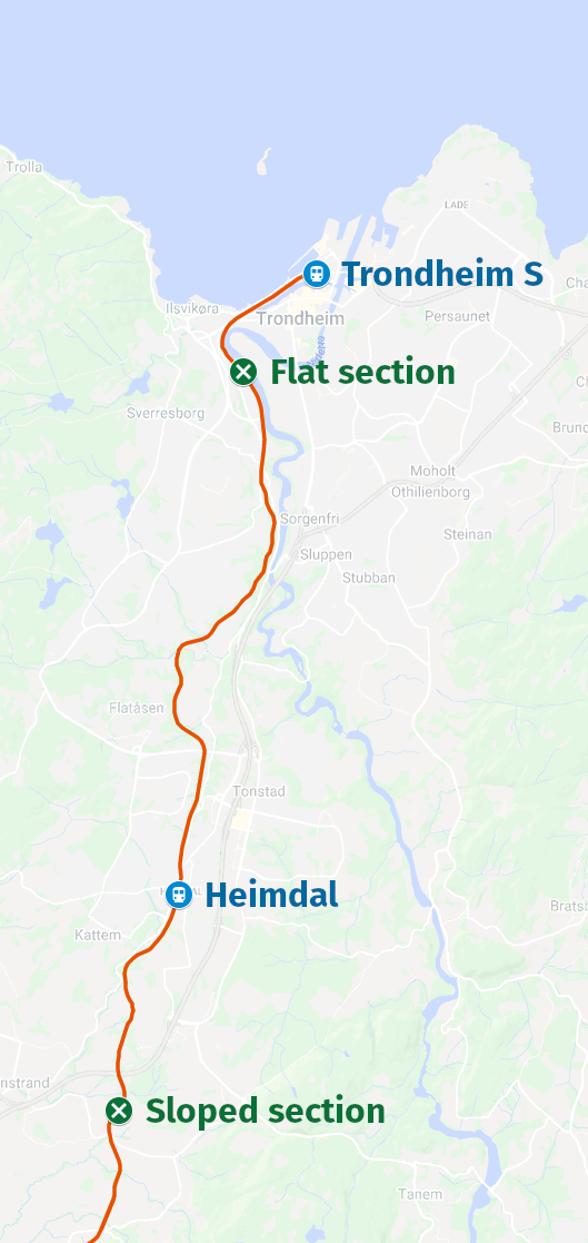
In order to properly demonstrate the viability of MFEH in railway, the coils were subsequently tested in a real-world scenario. The field setup, similar to that of the lab tests, is depicted in Figure 10a. For practical reasons, the coils were only tested along Norwegian railway, for which the electrification frequency is $16$ $\nicefrac{{2}}{{3}}$ $\mathrm{Hz}$ . Highlighted on the map in Figure 10b, two different test sites were used: a flat section of railway south of Trondheim Central station (Trondheim S), and an inclined section with a slope of $18\text{\,}\mathrm{\text{\textperthousand}}$ ( $1.8\text{\,}\mathrm{\%}$ ) south of Heimdal station.

The installation procedure was completed quickly and effortlessly; only about 10 minutes passed from the point where access to the section of railway was granted until the harvesting system was fully deployed and traffic could resume. This speaks to the ease of installation and non-invasiveness of MFEH along railway. Since access to the electrification system itself is not necessary, a condition monitoring system employing MFEH can be quickly installed with minimal impact on railway traffic. The installed system is pictured in Figure 11.

VI-A Results and discussion

The system was placed in each location for approximately two days, continuously recording the power output from the energy harvesting coils. The envelope of the output voltage indicates when a train draws current, and its magnitude is a result of the amount of current drawn by the locomotive, and—due to ground leakage currents—the locomotive’s distance to the harvester coil. The signal was matched with the train schedules to determine which train passed at which point in time. Shown in Figure 12 are two representative intervals from the recorded data, one from each test site.

(a) Flat section

(b) Sloped section

Fig. 12: The closed-loop voltage

V_{\ell}

across an impedance-matched load was recorded as trains passed by. The instantaneous dissipated power was derived as

P_{\ell}=\nicefrac{{V_{\ell}^{2}}}{{R_{\ell}}}

. In , a passenger train followed a few minutes later by a freight train both depart from Trondheim S, drawing relatively short bursts of current. Chart shows how a freight train sustains a larger current draw in order to maintain speed up the

18\text{\,}\mathrm{\text{\textperthousand}}

slope.

As illustrated in Figure 10b, the flat section is situated just $2.35\text{\,}\mathrm{km}$ south of Trondheim S, which means that trains running past in either direction will not draw a substantial amount of current. Northbound trains are arriving at the station and therefore generally do not draw current, while southbound trains are leaving the station and limited to a speed of $30\text{\,}\mathrm{km/h}$ . According to the daily schedule, the trains recorded in Figure 12a are both southbound trains leaving the station—one passenger and one freight.

Figure 12b shows the output from the energy harvester as a northbound freight train passes by up the $18\text{\,}\mathrm{\text{\textperthousand}}$ slope. The rail current is in the same order of magnitude as that seen for the flat section, albeit maintained at higher levels for a considerably longer duration of time. Compared to the short bursts of current in Figure 12a, a substantial current is drawn for about 9 minutes. In this location, only northbound trains, i.e. those running up the sloped section, will draw a significant current. It is presumably locations like this in which MFEH will be most effective.

VI-A1 Power and energy output

In Figure 12a, the voltage induced in Coil A by the passenger train peaks at $2\text{\,}\mathrm{V}$ amplitude, resulting in an instantaneous power output of $233\text{\,}\mathrm{\SIUnitSymbolMicro W}$ . For the freight train passing by a few minutes later, the peak induced voltage is $4.17\text{\,}\mathrm{V}$ and the power output $1.01\text{\,}\mathrm{mW}$ . For Coil B, the power figures are approximately halved— $169\text{\,}\mathrm{\SIUnitSymbolMicro W}$ and $569\text{\,}\mathrm{\SIUnitSymbolMicro W}$ for the passenger and freight trains, respectively.

Comparing Figures 12a and 12b, it is evident that the peak voltages induced by the two freight trains are similar. However, the power output from the sloped section is sustained for a substantially longer time. Accumulating the power output as the freight train passes by the sloped section gives a figure of $109\text{\,}\mathrm{mJ}$ and $80.4\text{\,}\mathrm{mJ}$ for Coils A and B, respectively.

Typically, around nine northbound freight trains pass by this point every day, which—through extrapolation—renders a daily energy harvest of around $981\text{\,}\mathrm{mJ}$ and $724\text{\,}\mathrm{mJ}$ for Coils A and B, respectively. When accounting for the four northbound electric passenger trains that also pass by ( $40\text{\,}\mathrm{mJ}$ and $26\text{\,}\mathrm{mJ}$ per train), the estimates become $1.14\text{\,}\mathrm{J}$ and $828\text{\,}\mathrm{mJ}$ per day for Coils A and B. Both coils therefore seem to be viable solutions for powering condition monitoring systems along railway. [10] reports instances of structural health monitoring systems requiring as little as $132\text{\,}\mathrm{mJ}$ per day, a little less than one tenth of the amount generated by Coil A on the sloped section.

The location of the energy harvester substantially impacts the amount of energy that can be scavenged. It was shown that a steeper incline increases the power output, although unless regenerative braking is used, only trains running up the slope will provide a significant rail current. Apart from the slope, there are several other factors at play. The current return path will generally be directed towards the closest power substation, which means that only when the harvester is located between the locomotive and the substation will there be a substantial current in the rails. Placing the coil close to a power substation will therefore presumably increase average power output.

It should be noted that for both in situ tests, the coils were placed $0.5\text{\,}\mathrm{m}$ from the rail due to restrictions placed on the height of trackside equipment. If the coils were constructed in a more compact form-factor, they could have been placed much closer to the rail, and—as seen in the laboratory trials—provided a substantially larger power output.

VII Conclusions

In this article, magnetic field energy harvesting (MFEH) in railway was modelled, tested, and demonstrated in situ. Initially, models were derived for the magnetic fields encountered in railway and the power output of an MFEH device. Following this modelling effort, two prototype energy harvesting coils were constructed, testing of which was performed in a controlled laboratory environment to validate their designs and verify the model. In the laboratory, the largest harvester rendered a power output of $40.5\text{\,}\mathrm{mW}$ when placed a distance of $0.25\text{\,}\mathrm{m}$ from a $50\text{\,}\mathrm{Hz}$ rail current of $200\text{\,}\mathrm{A}$ . Ultimately, both energy harvesters were placed in situ at two points along Norwegian railway to record real-world performance. The results make a convincing case for viability of MFEH in railway, with one coil harvesting approximately $0.1\text{\,}\mathrm{J}$ from a single freight train passing by up a sloped section. Depending on the number of trains passing by, the estimated daily output is in excess of $1\text{\,}\mathrm{J}$ —a sufficient energy budget for a low-power sensor node.

The power output was shown to be dependent on a number of factors, chief among them the magnitude and duration of the rail current. The amount of energy that can be harvested is therefore governed by the location of the system, the railway topology, as well as the amount traffic. Other factors include the coil’s distance to the rail and the magnetic properties of the core. It is expected that the power output may be substantially improved by increasing the core’s effective permeability, and by employing designs that allow placement closer to the rails.

This article provides the first known in situ demonstration of MFEH in railway. The concept lends itself to a quick, cost-effective, and non-invasive installation procedure, and could therefore be an attractive approach for railway administrations to extend the lifetime of battery-powered condition monitoring systems. Furthermore, the magnetic fields encountered in railway serve as a predictable source of energy, permitting power management optimisation techniques to employ train schedules to further improve energy consumption of trackside equipment.

References

[1] Publications Office of the European Union, “EU transport in figures,” Luxembourg, 2018.
[2] Norwegian Railway Directorate, “Jernbanestatistikk 2018,” Oslo, Norway, 2019, (in Norwegian).
[3] H. Akkermans, L. Besselink, L. van Dongen, and R. Schouten, “Smart Moves for Smart Maintenance,” in World Class Maintenance, 2016.
[4] Bane NOR (Norwegian National Rail Administration), “We create the railway of the future,” Oslo, Norway, 2017.
[5] M. Takikawa, “Innovation in railway maintenance utilizing information and communication technology (smart maintenance initiative).” Japan Railway & Transport Rev., no. 67, pp. 22–35, 2016.
[6] V. J. Hodge, S. O’Keefe, M. Weeks, and A. Moulds, “Wireless Sensor Networks for Condition Monitoring in the Railway Industry: A Survey,” IEEE Trans. Intell. Transp. Syst., vol. 16, no. 3, pp. 1088–1106, Jun. 2015.
[7] I. F. Akyìldìz, W. Su, Y. Sankarasubramaniam, and E. Çayırcı, “Wireless sensor networks: A survey,” Comput. Netw., vol. 38, no. 4, pp. 393–422, Mar. 2002.
[8] D. E. Boyle, M. E. Kiziroglou, P. D. Mitcheson, and E. M. Yeatman, “Energy Provision and Storage for Pervasive Computing,” IEEE Pervasive Comput., vol. 15, no. 4, pp. 28–35, Oct. 2016.
[9] A. Gjerstad, Bane NOR (Norwegian National Rail Administration), Aug. 2020, personal communication.
[10] K. S. Adu-Manu, N. Adam, C. Tapparello, H. Ayatollahi, and W. Heinzelman, “Energy-Harvesting Wireless Sensor Networks (EH-WSNs): A Review,” ACM Trans. Sensor Netw., vol. 14, no. 2, pp. 1–50, Apr. 2018.
[11] C. Ulianov, Z. Hadaš, P. Hyde, and J. Smilek, “Novel Energy Harvesting Solutions for Powering Trackside Electronic Equipment,” in Sustainable Rail Transport, M. Marinov and J. Piip, Eds. Cham, Switzerland: Springer, 2020.
[12] F. Yang, L. Du, H. Yu, and P. Huang, “Magnetic and Electric Energy Harvesting Technologies in Power Grids: A Review,” Sensors, vol. 20, no. 5, p. 1496, Apr. 2020.
[13] Y. Kuang, Z. J. Chew, T. Ruan, T. Lane, B. Allen, B. Nayar, and M. Zhu, “Magnetic field energy harvesting from the traction return current in rail tracks,” Applied Energy, vol. 292, pp. 1–14, Jun. 2021.
[14] A. E. Espe and G. Mathisen, “Towards Magnetic Field Energy Harvesting near Electrified Railway Tracks,” in 9th Mediterranean Conf. on Embedded Comput., Budva, Montenegro, 2020, pp. 1–4.
[15] S. Yuan, Y. Huang, J. Zhou, Q. Xu, C. Song, and P. Thompson, “Magnetic Field Energy Harvesting under Overhead Power Lines,” IEEE Trans. Power Electron., vol. 30, no. 11, pp. 6191–6202, Nov. 2015.
[16] S. Yuan, Y. Huang, J. Zhou, Q. Xu, C. Song, and G. Yuan, “A High-Efficiency Helical Core for Magnetic Field Energy Harvesting,” IEEE Trans. Power Electron., vol. 32, no. 7, pp. 5365–5376, Jul. 2017.
[17] W. Jiang, J. Lu, S. Hashimoto, and Z. Lin, “A non-intrusive magnetic energy scavanger for renewable power generation state monitoring,” in IEEE Int. Conf. on Renewable Energy Res. and Appl., Birmingham, UK, 2016, pp. 562–566.
[18] Z. Wu, D. S. Nguyen, R. M. White, P. K. Wright, G. O’Toole, and J. R. Stetter, “Electromagnetic energy harvester for atmospheric sensors on overhead power distribution lines,” J. of Phys.: Conf. Ser., vol. 1052, no. 1, pp. 1–4, Jul. 2018.
[19] A. Pourghodrat, C. A. Nelson, S. E. Hansen, V. Kamarajugadda, and S. R. Platt, “Power harvesting systems design for railroad safety,” Proc. of the Institution of Mech. Engineers, Part F: J. of Rail and Rapid Transit, vol. 228, no. 5, pp. 504–521, Apr. 2014.
[20] M. Wischke, M. Masur, M. Kröner, and P. Woias, “Vibration harvesting in traffic tunnels to power wireless sensor nodes,” Smart Materials and Structures, vol. 20, no. 8, p. 085014, Aug. 2011.
[21] Community Research and Development Information Service, “Greenrail, innovative and sustainable railway sleepers: the greener solution for railway sector ,” 2016, Proj. No.: 738373—H2020-SMEINST-2-2016-2017. [Online]. Available: https://cordis.europa.eu/project/id/738373
[22] S. Nandan, S. Thakare, K. Kulkarni, H. Wagh, and G. Magre, “T-BOX Wind Power Generation,” in 7th Intl. Conf. on Sci., Technol. & Manage., Nashik, India, 2017, pp. 148–156.
[23] H. Pan, H. Li, T. Zhang, A. A. Laghari, Z. Zhang, Y. Yuan, and B. Qian, “A portable renewable wind energy harvesting system integrated S-rotor and H-rotor for self-powered applications in high-speed railway tunnels,” Energy Conversion and Management, vol. 196, pp. 56–68, Sep. 2019.
[24] F. Kiessling, R. Puschmann, A. Schmieder, and E. Schneider, Contact Lines for Electric Railways, 1st ed. Munich, Germany: Publicis, 2001.
[25] F. Nilsen, “Sporstrømmer og potensialer i kontaktledningsanlegg,” Jernbaneverket, Tech. Rep., 1997, (in Norwegian).
[26] R. Ahmed, B. Buchli, S. Draskovic, L. Sigrist, P. Kumar, and L. T. Takikawa, “Optimal Power Management with Guaranteed Minimum Energy Utilization for Solar Energy Harvesting Systems,” ACM Trans. on Embedded Comput. Syst., vol. 18, no. 4, p. 30, Jun. 2019.
[27] J.-H. Lee, J.-H. Kim, and Y.-G. Park, “Review of Minimum Curve Radius and Cant Range Setting for Mixed Section of Low and High speed Trains in Conventional Railway Line ,” Journal of the Korea Academia – Industrial Cooperation Society, vol. 21, no. 10, pp. 345–353, Oct. 2020.
[28] R. S. Carmichael, Ed., Handbook of the Physical Properties of Rocks: Volume II. Boca Raton, FL, USA: CRC Press, 1982.
[29] D. Jiles, Introduction to Magnetism and Magnetic Materials, 3rd ed. Boca Raton, FL, USA: CRC Press, 2016.
[30] N. M. Roscoe and M. D. Judd, “Harvesting Energy from Magnetic Fields to Power Condition Monitoring Sensors,” IEEE Sensors J., vol. 13, no. 6, pp. 2263–2270, Jun. 2013.
[31] S. W. Wright, M. E. Kiziroglou, S. Spasic, N. Radosevic, and E. M. Yeatman, “Inductive Energy Harvesting From Current-Carrying Structures,” IEEE Sensors Lett., vol. 3, no. 6, pp. 1–4, Jun. 2019.
[32] Ferroxcube, “4B1 Material Specification,” 2008. [Online]. Available: https://elnamagnetics.com/wp-content/uploads/library/Ferroxcube-Materials/4B1_Material_Specification.pdf
[33] K. Tashiro, H. Wakiwaka, and G.-Y. Hattori, “Estimation of Effective Permeability for Dumbbell-Shaped Magnetic Cores,” IEEE Trans. Magn., vol. 51, no. 1, pp. 1–4, Jan. 2015.
[34] B. I. Olsen, Bane NOR (Norwegian National Rail Administration), Mar. 2020, personal communication.