Skillearn: Machine Learning Inspired by Humans’ Learning Skills
Abstract
Humans, as the most powerful learners on the planet, have accumulated a lot of learning skills, such as learning through tests, interleaving learning, self-explanation, active recalling, to name a few. These learning skills and methodologies enable humans to learn new topics more effectively and efficiently. We are interested in investigating whether humans’ learning skills can be borrowed to help machines to learn better. Specifically, we aim to formalize these skills and leverage them to train better machine learning (ML) models. To achieve this goal, we develop a general framework – Skillearn, which provides a principled way to represent humans’ learning skills mathematically and use the formally-represented skills to improve the training of ML models. In two case studies, we apply Skillearn to formalize two learning skills of humans: learning by passing tests and interleaving learning, and use the formalized skills to improve neural architecture search. Experiments on various datasets show that trained using the skills formalized by Skillearn, ML models achieve significantly better performance.
1 Introduction
Given a group of human students, assuming they work equally hard, there are three major factors determining which students learn better than others, including intelligence, learning skills, and learning materials. People with higher intelligence quotient (IQ) are stronger learners. Learning materials, such as textbooks, video lectures, practice questions, etc. are also crucial in determining the quality of learning. Another vital factor impacting learning outcomes is learning skills. Oftentimes, students in the same class have similar IQ and have access to the same learning materials, but their final grades (which measure learning quality) have a large variance. The major differentiating factor is that different students have different levels of mastery of learning skills. Some students have better learning methodologies, which enable them to learn faster and better. In the long history of learning, humans have accumulated a lot of effective learning skills, such as learning through tests, interleaving learning, self-explanation, active recalling, etc.

Similar to human learning, the performance of machine learning (ML) models is also determined by several factors. In the current practice of ML, two dominant factors determining ML performance are the capacity of models and the abundance of data. ML model capacity is analogous to the intelligence of humans. From linear models such as support vector machine to nonlinear models such as deep neural networks, ML researchers have been continuously building more powerful ML models to deal with more complicated tasks. It is like the evolution of humans’ brains, which become increasingly intelligent. Data for ML is analogous to learning materials for humans. ML models trained with more labeled data in general perform better.
For intelligence and learning materials in human learning (HL), we identify their counterparts in machine learning as model capacity and data. We are interested in asking: for learning skills in HL, do they have counterparts in ML as well? Can machines be equipped with effective learning skills as humans are? In this paper, we aim to address these questions. We propose a general framework – Skillearn, which draws inspiration from humans’ learning skills and formulates them into machines’ learning skills (MLS). These MLS are leveraged to train better ML models. In Skillearn, there are one or multiple learner models, each with one or multiple sets of learnable parameters such as weight parameters, architectures, hyperparameters, etc. Different learners interact with each other through interaction functions. The learning of all learners is organized into multiple stages, each involving a subset of learners. The stages have an order, but they are performed end-to-end in a multi-level optimization framework where latter stages influence earlier stages and vice versa. We develop a unified optimization algorithm for solving the multi-level optimization problem in Skillearn. In two case studies, we apply Skillearn to formalize two learning skills of humans – learning by passing tests (LPT) and interleaving learning (IL) – into machines’ learning skills (MLS) and leverage these MLS for neural architecture search (Zoph and Le 2017; Real et al. 2019; Liu et al. 2019). In LPT, a tester model dynamically creates tests with increasing levels of difficulty to evaluate a testee model; the testee continuously improves its architecture by passing however difficult tests created by the tester. In IL, a set of models collaboratively learn a data encoder in an interleaving fashion: the encoder is trained by model 1 for a while, then passed to model 2 for further training, then model 3, and so on; after trained by all models, the encoder returns back to model 1 and is trained again, then moving to model 2, 3, etc. This process repeats for multiple rounds. Experiments on various datasets demonstrate that ML models trained by these two learning skills achieve significantly better performance.
The major contributions of this work are as follows.
- •
We propose to leverage the broadly-used and effective learning skills in human learning to develop better machine learning methods.
- •
We propose Skillearn, a general framework for formulating humans’ learning skills into machines’ learning skills that can be leveraged by ML models for achieving better learning outcomes.
- •
We apply Skillearn to formalize two skills in human learning – learning by passing tests (LPT) and interleaving learning (IL), and apply them to improve neural architecture search.
- •
On various datasets, we demonstrate the effectiveness of the two skills – LPT and IL formalized by Skillearn – in learning better neural architectures.
The rest of the paper is organized as follows. Section 2 presents the general Skillearn framework. In Section 3 and 4, we present two case studies, where Skillearn is applied to formalize two skills in human learning: learning by passing tests and interleaving learning. Section 5 reviews related works and Section 6 concludes the paper.
2 Skillearn: Machine Learning Inspired by Human’s Learning Skills
In this section, we present a general framework called Skillearn, which gets inspiration from humans’ learning skills, formalize these skills, and leverage them to improve machine learning. We begin with a brief overview of humans’ learning skills and summarize their properties. Then we present the Skillearn framework and the optimization algorithm for this framework.
2.1 Humans’ Learning Skills
Humans, as the most powerful learners on the planet, have accumulated a lot of skills and techniques in learning faster and better. Here are some examples.
- •
Learning through testing. After learning a topic, a student can solve some test problems (created or selected by a teacher) about this topic to identify the strong and weak points in his/her understanding of this topic, and re-learn the topic based on the identified strong and weak points. In re-learning, the identified strong and weak points help the student to know what to focus on. The quality of test problems plays a crucial role in effectively evaluating the student. How to create or select high-quality test problems is an important skill that the teacher needs to learn.
- •
Interleaving learning is a learning technique where a learner interleaves the studies of multiple topics: study topic for a while, then switch to , subsequently to ; then switch back to , and so on, forming a pattern of . Interleaving learning is in contrast to blocked learning, which studies one topic very thoroughly before moving to another topic. Compared with blocked learning, interleaving learning increases long-term retention and improves ability to transfer learned knowledge.
- •
Learning by ignoring. In course learning, given a large collection of practice problems provided in the textbook, the teacher selects a subset of problems as homework for the students to practice instead of using all problems in the textbook. Some practice problems are ignored because 1) they are too difficult which might confuse the students; 2) they are too simple which are not effective in helping the students to practice their knowledge learned during lectures; 3) they are repetitive.
2.1.1 Properties of Humans’ Learning Skills
From the above examples of humans’ learning skills, we observe the following properties of them.
- •
A learning event involves multiple learners. For example, in learning through testing, there are two learners: a student and a teacher. The teacher learns how to create test problems and the student learns how to solve these test problems.
- •
In a learning task, a learner has multiple aspects to learn about this task. For example, in learning by ignoring, to create effective homework problems, the teacher needs to learn: 1) how to solve these problems; 2) which problems are more valuable to use as homework.
- •
Different learners interact with each other during learning. For example, in learning through testing, the teacher creates test problems and uses them to evaluate the student.
- •
In a learning task, the learning process is divided into multiple stages. These stages have a certain order. Each stage involves a subset of learners. For example, in learning through testing, there are three stages: 1) the teacher learns a topic; 2) the teacher creates test problems about this topic and uses them to evaluate the student; 3) based on the strong and weak points identified during solving the test problems, the student re-learns this topic. The three stages have a sequential order and cannot be switched. The first stage involves the teacher only; the second stage involves both the teacher and the student; the third stage involves the student only.
- •
Testing and validation are widely used to evaluate the outcome of learning and provide feedback for improving learning. For example, in learning through testing, the student takes a test to identify the strong and weak points in his/her learning of a topic.
- •
Learning is performed on various learning materials, including textbooks used for initial learning, homeworks used for enhancing the understanding of knowledge learned from textbooks, tests used for evaluating the outcome of learning, etc.
2.2 General Framework of Skillearn

Based on the properties of humans’ learning skills, we propose a framework called Skillearn to formalize the learning skills of humans and incorporate them into machine learning. In Skillearn, we have the following elements.
- •
Learners. There could be one or multiple learners. Each learner is an ML model, such as a deep convolutional network, a deep generative model, a nonparametric kernel density estimator, etc. This is analogous to human learning which involves one or multiple human learners.
- •
Learnable parameters. Each learner has one or more sets of learnable parameters, which could be weight parameters of a network, architecture of a network, weights of training examples, hyperparameters, etc. This is analogous to human learning where each human learner learns multiple aspects in a learning task.
- •
Interaction function, which describes how two or more learners interact with others. Some examples of interaction include: 1) in knowledge distillation, given an unlabeled image dataset, model predicts the pseudo labels of these images; then model is trained using these images and the pseudo labels generated by model ; 2) given a set of texts, two text encoders and extract embeddings of the texts; and are tied together via distributional matching: the distribution of embeddings extracted by is encouraged to have small total-variance with the distribution of embeddings extracted by . This is analogous to human learning where multiple human learners interact with each other.
- •
Learning stages. The learning of all learners is not conducted at one shot simultaneously. The learning is performed at multiple stages with an order. At each stage, a subset of learners participate in the learning. For example, in knowledge distillation, there are two stages: 1) a teacher model is trained; 2) the teacher model predicts pseudo labels on an unlabeled dataset and the pseudo-labeled dataset is used to train the student model. The first stage involves a single learner, which is the teacher. The second stage involves two learners: the teacher and the student. This is analogous to human learning where the learning process is divided into multiple stages. Mathematically, we formulate the learning at each stage as an optimization problem. The outcome of one learning stage is passed to another learning stage via the interaction function.
- •
Validation stage. This stage evaluates the outcome of learning and provides feedback to improve the learning at the learning stages. This is analogous to the testing and validation in human learning. The validation stage is formulated as an optimization problem as well. The learning outcomes produced in the learning stages are passed to the validation stage.
- •
Datasets. Datasets in ML are analogous to learning materials in human learning. Each learner has a training dataset and a validation dataset. The training dataset is used in the learning stages and the validation dataset is used in the validation stage. Besides, there are auxiliary datasets (labeled or unlabeled) on which the learners interact with each other.
Next, we define the learning stages. Each learning stage performs a focused learning activity which is defined as an optimization problem. The optimization problem involves a training loss and (optionally) an interaction function which describes how the learners involved in this stage interact with each other. A learning stage consists of the following elements:
- •
Active learners. A subset of learners (one or more) are involved at this learning stage. These learners are called active learners.
- •
Active learnable parameters. For each active learner, a sub-collection of its learnable parameter sets are trained in this stage.
- •
Supporting learnable parameters. For each active learner, a sub-collection of its learnable parameter sets are used to define the loss function and interaction function, but they are not updated at this stage.
- •
Active training datasets, which include the training dataset of every active learner.
- •
Active auxiliary datasets, which include the auxiliary datasets where the interaction function in this learning stage is defined on.
- •
Training loss, which is defined on the active training data collection, active learnable parameters, and supporting learnable parameters.
- •
Interaction function, which depicts the interaction between two or more active learners. It is defined on the active auxiliary datasets, active learnable parameters, and supporting learnable parameters.
In Skillearn, there is a single validation stage where an optimization problem is defined. The optimization problem involves one or more validation losses and (optionally) an interaction function which describes how the learners in the validation stage interact with each other. The validation stage consists of the following elements.
- •
Active learners, which are the learners to validate.
- •
Remaining learnable parameters. At each learning stage, a subset of parameters are learned. After all learning stages, the parameters that have not been learned are called remaining parameters. The remaining parameters are updated in the validation stage.
- •
Validation datasets: validation datasets of all active learners.
- •
Active auxiliary datasets, which include the auxiliary datasets where the interaction function in the validation stage is defined on.
- •
Validation losses, which are defined on remaining learnable parameters, validation datasets, and (optionally) active auxiliary datasets.
- •
Interaction function, which depicts the interaction between two or more active learners. It is defined on remaining learnable parameters and active auxiliary datasets.
2.2.1 Mathematical Setup
| Notation | Meaning |
|---|---|
| Number of learners | |
| Training data of the -th learner | |
| Validation data of the -th learner | |
| Auxiliary datasets accessible to all learners | |
| Number of learnable parameter sets belonging to the -th learner | |
| The -th learnable parameter set of the -th learner | |
| Number of learning stages | |
| Number of active learners in the -th learning stage | |
| The set of active learners in the -th learning stage | |
| The -th active learner in the -th learning stage | |
| The number of active parameter sets of the -th active learner in the -th learning stage | |
| The -th active parameter set of the -th learner in the -th learning stage | |
| The collection of active parameter sets of the -th active learner in the -th learning stage | |
| All active parameter sets in the -th learning stage | |
| The number of supporting parameter sets of the -th active learner in the -th learning stage | |
| The -th supporting parameter set of the -th active learner in the -th learning stage | |
| The collection of supporting parameter sets of the -th active learner in the -th learning stage | |
| All supporting parameter sets in the -th learning stage | |
| Training dataset of the -th active learner in the -th learning stage | |
| Active training datasets in the -th learning stage | |
| Active auxiliary datasets in the -th learning stage | |
| Training loss in the -th learning stage | |
| Interaction function in the -th learning stage |
We assume there are learners in total. For each learner , it has a training set and optionally a validation set . Meanwhile, all learners share a common collection of auxiliary datasets , which could be unlabeled datasets used for self-supervised pretraining (He et al. 2019), additional labeled datasets used for validation, and so on. The learner has one or more sets of learnable parameters . The learnable parameters could be network weights, architectures, hyperparameters, weights of training examples, etc.
We assume there are learning stages. At each stage , a subset of learners are involved in the learning, which are called active learners. For each active learner , a sub-collection of its learnable parameter sets are trained at this stage, which are called active learnable parameters. Let denote the active learnable parameters for all active learners. Meanwhile, another sub-collection of its learnable parameter sets are used to define the training loss function and interaction function. But are not updated at this stage. They are called supporting learnable parameters. Let denote the supporting learnable parameters for all active learners. Let denote the active training datasets, consisting of the training dataset of each active learner in . Let denote the active auxiliary datasets used in this stage to define the interaction function. The learning activity at stage is formulated as an optimization problem where the optimization variables are active learnable parameters and the objective involves 1) a training loss defined on the active training datasets, active learnable parameters, and supporting learnable parameters; 2) (optionally) an interaction function that depicts the interaction between learners in . The notations are summarized in Table 1.
2.2.2 The Mathematical Framework for Skillearn
The formulation of Skillearn is shown in Eq.(1).
| (1) |
It is a multi-level optimization framework, which involves optimization problems. On the constraints are optimization problems, each corresponding to a learning stage. The learning stages are ordered. From bottom to top, the optimization problems correspond to the learning stage respectively. In the optimization problem of the learning stage , the optimization variables are the active learnable parameters of all active learners in this stage. The objective function consists of a training loss defined on the active learnable parameters , supporting learnable parameters , optimal solutions obtained in previous learning stages, active training datasets , and active auxiliary datasets . Typically, can be decomposed into a summation of active learners’ individual training losses:
| (2) |
where is the training loss of the active learner defined on its active parameters , supporting parameters , and training dataset . The learners do not interact in the training loss. The other part of the objective function is the interaction function which depicts how the active learners interact with each other in this learning stage. It is defined on the active learnable parameters , supporting learnable parameters , optimal solutions in previous stages, and active auxiliary datasets . is a tradeoff parameter between the training loss and interaction function. is needed to define the objective, but it is not updated at this stage. After completing the learning at stage , we obtain the optimal solution . Note that is function of since is a function of the objective and the objective is a function of . is used to define the objectives in later stages.
At the very top of Eq.(1), the optimization problem (outside the constraint block) corresponds to the validation stage which validates the optimal solutions obtained in the learning stages. The optimization variables are remaining learnable parameters that have not been learned in the learning stages. The objective function consists of a validation loss and an interaction function. is a tradeoff parameter. The validation loss is defined on the validation sets of all learners , the optimal solutions , and the auxiliary datasets . The interaction function is defined on and .
Remarks:
- •
Note that for simplicity, we assume the optimization problem at each stage is a minimization problem. The optimization problem can be more complicated problems such as min-max problems.
- •
At a certain stage, a learnable parameter cannot be simultaneously an active parameter and a supporting parameter. For active parameters in stage , once learned, they cannot be active parameters or supporting parameters in later stages. For supporting parameters in stage , they can be active parameters or supporting parameters in later stages.
- •
The supporting parameters are not learned in previous stages.
2.3 Optimization Algorithm for Skillearn
In this section, we develop an algorithm to solve the Skillearn problem in Eq.(1), inspired by the algorithm in (Liu et al. 2019). For each learning stage with an optimization problem: , we approximate the optimal solution by one-step gradient descent update of the variable :
| (3) |
In learning stages , may be used to define objective functions. For a stage where , if its objective involves , we replace with and get an approximated objective. When approximating , we use the gradient of the approximated objective:
| (4) |
For the objective in the validation stage, it can be approximated as:
| (5) |
We update the remaining learnable parameters by minimizing this approximated objective. The optimization algorithm for Skillearn is summarized in Algorithm 1.
3 Case Study I: Learning by Passing Tests
In this section, we apply our general Skillearn framework to formalize a human learning technique – learning by passing tests, and apply it to improve machine learning. In human learning, an effective and widely used methodology for improving learning outcome is to let the learner take increasingly more-difficult tests. To successfully pass a more challenging test, the learner needs to gain better learning ability. By progressively passing tests that have increasing levels of difficulty, the learner strengthens his/her learning capability gradually.
Inspired by this test-driven learning technique of humans, we are interested in investigating whether this methodology is helpful for improving machine learning as well. We use the Skillearn framework to formalize this human learning technique, which results in a novel machine learning framework called learning by passing tests (LPT). In this framework, there are two learners: a “testee” model and a “tester” model. The tester creates a sequence of “tests” with growing levels of difficulty. The testee tries to learn better so that it can pass these increasingly more-challenging tests. Given a large collection of data examples called “test bank”, the tester creates a test by selecting a subset of examples from the test bank. The testee applies its intermediately-trained model to make predictions on the examples in . The prediction error rate reflects how difficult this test is. If the testee can make correct predictions on , it means that is not difficult enough. The tester will create a more challenging test by selecting a new set of examples from the test bank in a way that the new error rate achieved by is larger than . Given this more demanding test , the testee re-learns its model to pass , in a way that the newly-learned model achieves a new error rate on where is smaller than . This process iterates until convergence.
In our framework, both the testee and tester perform learning. The testee learns how to best conduct a target task and the tester learns how to create difficult and meaningful tests. To encourage a created test to be meaningful, the tester trains a model using to perform a target task . If the model performs well on , it indicates that is meaningful. The testee has two sets of learnable parameters: neural architecture and network weights. The tester has three learnable modules: data encoder, test creator, and target-task executor. The learning is organized into three stages. In the first stage, the testee trains its network weights on the training set of task with the architecture fixed. In the second stage, the tester trains its data encoder and target-task executor on a created test to perform the target task , with the test creator fixed. In the third stage, the testee updates its model architecture by minimizing the predictive loss on the test created by the tester; the tester updates its test creator by maximizing and minimizing the loss on the validation set of . The testee and tester interact on the loss function in an adversarial manner, where the testee minimizes this loss while the tester maximizes this loss. The three stages are performed jointly end-to-end in a multi-level optimization framework, where a latter stage influences an earlier stage and vice versa. We apply our method for neural architecture search (Zoph and Le 2017; Liu et al. 2019; Real et al. 2019) in image classification tasks on CIFAR-100, CIFAR-10, and ImageNet (Deng et al. 2009). Our method achieves significant improvement over state-of-the-art baselines.
3.1 Method
In this section, we describe how to instantiate the general Skillearn framework to the LPT framework, and how to instantiate the general optimization procedure of Skillearn to a specialized optimization algorithm for LPT.
3.1.1 Learning by Passing Tests
In the learning by passing tests (LPT) framework, there are two learners: a testee model and a tester model, where the testee studies how to perform a target task such as classification, regression, etc. The eventual goal is to make the testee achieve a better learning outcome with the help of the tester. There is a collection of data examples called “test bank”. The tester creates a test by selecting a subset of examples from the test bank. Given a test , the testee applies its intermediately-trained model to make predictions on and measures the prediction error rate . From the perspective of the tester, indicates how difficult the test is. If is small, it means that the testee can easily pass this test. Under such circumstances, the tester will create a more difficult test which renders the new error rate achieved by on is larger than . From the testee’s perspective, indicates how well the testee performs on the test. Given this more difficult test , the testee refines its model to pass this new test. It aims to learn a new model in a way that the error rate achieved by on is smaller than . This process iterates until an equilibrium is reached. In addition to being difficult, the created test should be meaningful as well. It is possible that the test bank contains poor-quality examples where the class labels may be incorrect or the input data instances are outliers. Using an unmeaningful test containing poor-quality examples to guide the learning of the testee may render the testee to overfit these bad-quality examples and generalize poorly on unseen data. To address this problem, we encourage the tester to generate meaningful tests by leveraging the generated tests to perform a target task (e.g., classification). Specifically, the tester uses examples in the test to train a model for performing . If the performance (e.g., accuracy) achieved by this model in conducting is high, the test is considered to be meaningful. The tester aims to create a test that can yield a high .
| Notation | Meaning |
|---|---|
| Architecture of the testee | |
| Network weights of the testee | |
| Data encoder of the tester | |
| Test creator of the tester | |
| Target-task executor of the tester | |
| Training data of the testee | |
| Training data of the tester | |
| Validation data of the tester | |
| Test bank |
In our framework, both the testee and the tester performs learning. The testee studies how to best fulfill the target task . The tester studies how to create tests that are difficult and meaningful. In the testee’ model, there are two sets of learnable parameters: model architecture and network weights. The architecture and weights are both used to make predictions in . The tester’s model performs two tasks simultaneously: creating tests and performing target-task . The model has three modules with learnable parameters: data encoder, test creator, and target-task executor, where the test creator performs the task of generating tests and the target-task executor conducts . The test creator and target-task executor share the same data encoder. The data encoder takes a data example as input and generates a latent representation for this example. Then the representation is fed into the test creator which determines whether should be selected into the test. The representation is also fed into the target-task executor which performs prediction on during performing the target task .
| Active learners | Testee |
|---|---|
| Active learnable parameters | Network weights of the testee |
| Supporting learnable parameters | Architecture of the testee |
| Active training datasets | Training dataset of target-task performed by the testee |
| Active auxiliary datasets | – |
| Training loss | Training loss of target-task : |
| Interaction function | – |
| Optimization problem |
| Active learners | Examiner |
|---|---|
| Active learnable parameters | 1) Data encoder of the tester; 2) Target-task executor of the tester. |
| Supporting learnable parameters | Test creator of the tester |
| Active training datasets | Training data of target-task performed by the tester |
| Active auxiliary datasets | Test bank |
| Training loss | |
| Interaction function | – |
| Optimization problem |
In our framework, the learning of the testee and the tester is organized into three stages. In the first stage, the testee learns its network weights by minimizing the training loss defined on the training data in the task . The architecture is used to define the training loss, but it is not learned in this stage. If is learned by minimizing this training loss, a trivial solution will be yielded where is very large and complex that it can perfectly overfit the training data but will generalize poorly on unseen data. Let denotes the optimally learned in this stage. Note that is a function of because is a function of the training loss and the training loss is a function of . Table 3 shows the key elements of this learning stage under the Skillearn terminology. The testee is the active learner, which performs learning in this stage. Network weights of the testee are the active learnable parameters, which are updated at this stage. The architecture variables of the testee are the supporting learnable parameters, which are used to define the loss function, but are not updated at this stage. Active training datasets include the training data of the task performed by the testee. There are no active auxiliary datasets. Training loss is . There is no interaction function at this stage. The optimization problem is:
| (6) |
In the second stage, the tester learns its data encoder and target-task executor by minimizing the training loss in the task . The training loss consists of two parts. The first part is defined on the training dataset in . The second part is defined on the test created by the test creator. For each example in the test bank , it is first fed into the encoder , then the creator , which outputs a binary value indicating whether should be selected into the test. is the collection of examples whose binary value is equal to 1. is a tradeoff parameter between these two parts of losses. The creator is used to define the second-part loss, but it is not learned in this stage. Otherwise, a trivial solution will be yielded where always sets the binary value to 0 for each test-bank example so that the second-part loss becomes 0. Let and denote the optimally trained and in this stage. Note that they are both functions of since they are functions of the training loss and the training loss is a function of . Table 4 shows the key elements of this learning stage under the Skillearn terminology. The tester is the active learner. The active learnable parameters include the data encoder and target-task executor of the tester. The supporting learnable parameters include the test creator. The active training datasets include the training data of target-task performed by the tester. The active auxiliary datasets include the test bank. The training loss is . There is no interaction function at this stage. The optimization problem is:
| (7) |
| Active learners | Testee, tester |
|---|---|
| Remaining learnable parameters | 1) Architecture of the testee; 2) Test creator of the tester |
| Validation datasets | Validation dataset of the tester |
| Active auxiliary datasets | Test bank |
| Validation loss | |
| Interaction function | Testee’s prediction loss defined on the test created by the tester: |
| Optimization problem |
In the third stage, the testee learns its architecture by trying to pass the test created by the tester. Specifically, the testee aims to minimizes the predictive loss of its model on the test:
| (8) |
where is an example in the test and is the loss defined in this example. A smaller indicates that the testee performs well on this test. Meanwhile, the tester learns its test creator in a way that can create a test with more difficulty and meaningfulness. Difficulty is measured by the testee’s predictive loss on the test. Given a model of the testee and two tests of the same size (same number of examples): created by and created by , if , it means that is more challenging to pass than . Therefore, the tester can learn to create a more challenging test by maximizing . A trivial solution of increasing is to enlarge the size of the test. But a larger size does not imply more difficulty. To discourage this degenerated solution from happening, we normalize the loss using the size of the test:
| (9) |
where is the cardinality of the set . Under the Skillearn terminologies, the loss in Eq.(9) is the interaction function where the testee and tester interact. The testee aims to minimize this loss to “pass” the testee and the tester aims to maximize this loss to “fail” the testee. To measure the meaningfulness of a test, we check how well the optimally-trained task executor and data encoder of the tester perform on the validation data in the target task , and the performance is measured by the validation loss: . and are trained using the test generated by in the second stage. If the validation loss is small, it means that the created test is helpful in training the task executor and therefore is considered as being meaningful. To create a meaningful test, the tester learns by minimizing . In sum, is learned by maximizing , where is a tradeoff parameter between these two objectives. Under the Skillearn terminology, this stage is a validation stage. Table 5 summarizes the key elements of this stage. The active learners include both the testee and the tester. The remaining learnable parameters include the architecture of the testee and the test creator of the tester. The validation datasets include the validation data in the target-task performed by the tester. The active auxiliary datasets include the test bank. The validation loss is . The interaction function is . The optimization problem is:
| (10) |
| Skillearn | Learning by Passing Tests |
|---|---|
| Learners | 1) Testee; 2) Tester |
| Learnable parameters | 1) Architecture of testee; 2) Network weights of testee; 3) Data encoder of tester; 4) Target-task executor of tester; 5) Test creator of tester. |
| Interaction function | Testee’s prediction loss defined on the test created by the tester: |
| Learning stages |
Learning stage I: the testee learns its network weights on its training data:
Learning stage II: the tester uses its test creator to select a subset of examples from the test bank, then it learns its data encoder and target-task executor on its training data and on the selected examples from the test bank: |
| Validation stage | 1) The testee updates its architecture to minimize the prediction loss on the test created by the tester; 2) The tester updates its test creator to maximize the testee’s prediction loss and minimize its own validation loss. |
| Datasets | 1) Training data of the testee; 2) Training data of the tester; 3) Validation data of the tester; 4) Test bank. |
The three stages are mutually dependent: learned in the first stage and and learned in the second stage are used to define the objective function in the third stage; the updated and in the third stage in turn change the objective functions in the first and second stage, which subsequently render , , and to be changed. Putting these pieces together, we instantiate the Skillearn framework into the following LPT formulation:
| (11) |
This formulation nests three optimization problems. On the constraints of the outer optimization problem are two inner optimization problems corresponding to the first and second learning stage respectively. The objective function of the outer optimization problem corresponds to the validation stage. Table 6 summarizes the instantiation of Skillearn to LPT.
As of now, the test is represented as a subset, which is highly discrete and therefore difficult for optimization. To address this problem, we perform a continuous relaxation of :
| (12) |
where for each example in the test bank, the original binary value indicating whether should be selected is now relaxed to a continuous probability representing how likely should be selected. Under this relaxation, can be computed as follows:
| (13) |
where we calculate the loss on each test-bank example and weigh this loss using . If is small, it means that is less likely to be selected into the test and its corresponding loss should be down-weighted. Similarly, is calculated as . And can be calculated as
| (14) |
Similar to (Liu et al. 2019), we represent the architecture of the testee in a differentiable way. The search space of is composed of a large number of building blocks. The output of each block is associated with a variable indicating how important this block is. After learning, blocks whose is among the largest are retained to form the final architecture. In this end, architecture search amounts to optimizing the set of architecture variables .
3.1.2 Optimization Algorithm
In this section, we instantiate the general optimization framework in Section 2.3 to derive an optimization algorithm for LPT. We approximate and using one-step gradient descent update of and with respect to and approximate using one-step gradient descent update of with respect to . Then we plug in these approximations into
| (15) |
and perform gradient-descent update of and with respect to this approximated objective. In the sequel, we use to denote .
Approximating using where is a learning rate and simplifying the notation of as , we can calculate the approximated gradient of w.r.t as:
| (16) |
The second term in the third line involves expensive matrix-vector product, whose computational complexity can be reduced by a finite difference approximation:
| (17) |
where and is a small scalar that equals . We approximate and using the following one-step gradient descent update of and respectively:
| (18) |
where and are learning rates. Plugging in these approximations into the objective function in Eq.(15), we can learn by maximizing the following objective using gradient methods:
| (19) |
The derivative of the second term in this objective with respect to can be calculated as:
| (20) |
where
| (21) |
Similar to Eq.(17), using finite difference approximation to calculate
and , we have:
| (22) |
where and . For the first term in the objective, we can use chain rule to calculate its derivative w.r.t , which involves calculating the derivative of and w.r.t to . The derivative of w.r.t can be calculated as:
| (23) |
where is given in Eq.(21) and
can be approximated with ,
where is . The derivative of w.r.t can be calculated as
| (24) |
where is given in Eq.(21). The algorithm for solving LPT is summarized in Algorithm 2.
not converged
1. Update the architecture of the testee by descending the gradient calculated in Eq.(16)
2. Update the test creator of the tester by ascending the gradient calculated in Eq.(20-24)
3. Update the data encoder and target-task executor of the tester using Eq.(18)
4. Update the weights of the testee by descending
3.2 Experiments
We apply LPT for neural architecture search in image classification tasks. Following (Liu et al. 2019), we first perform architecture search which finds out an optimal cell, then perform architecture evaluation which composes multiple copies of the searched cell into a large network, trains it from scratch, and evaluates the trained model on the test set. We let the target task of the learner and that of the tester be the same.
3.2.1 Datasets
We used three datasets in the experiments: CIFAR-10, CIFAR-100, and ImageNet (Deng et al. 2009). The CIFAR-10 dataset contains 50K training images and 10K testing images, from 10 classes (the number of images in each class is equal). Following (Liu et al. 2019), we split the original 50K training set into a new 25K training set and a 25K validation set. In the sequel, when we mention “training set”, it always refers to the new 25K training set. During architecture search, the training set is used as the training data of the learner and the training data of the tester. The validation set is used as the test bank and the validation data of the tester. During architecture evaluation, the combination of the training data and validation data is used to train the large network stacking multiple copies of the searched cell. The CIFAR-100 dataset contains 50K training images and 10K testing images, from 100 classes (the number of images in each class is equal). Similar to CIFAR-100, the 50K training images are split into a 25K training set and 25K validation set. The usage of the new training set and validation set is the same as that for CIFAR-10. The ImageNet dataset contains a training set of 1.2M images and a validation set of 50K images, from 1000 object classes. The validation set is used as a test set for architecture evaluation. Following (Liu et al. 2019), we evaluate the architectures searched using CIFAR-10 and CIFAR-100 on ImageNet: given a cell searched using CIFAR-10 and CIFAR-100, multiple copies of it compose a large network, which is then trained on the 1.2M training data of ImageNet and evaluated on the 50K test data.
3.2.2 Experimental Settings
Our framework is a general one that can be used together with any differentiable search method. Specifically, we apply our framework to the following NAS methods: 1) DARTS (Liu et al. 2019), 2) P-DARTS (Chen et al. 2019), 3) DARTS+ (Liang et al. 2019b), 4) DARTS- (Chu et al. 2020a). The search space in these methods are similar. The candidate operations include: and separable convolutions, and dilated separable convolutions, max pooling, average pooling, identity, and zero. In LPT, the network of the learner is a stack of multiple cells, each consisting of 7 nodes. For the data encoder of the tester, we tried ResNet-18 and ResNet-50 (He et al. 2016b). For the test creator and target-task executor, they are set to one feed-forward layer. and are both set to 1.
For CIFAR-10 and CIFAR-100, during architecture search, the learner’s network is a stack of 8 cells, with the initial channel number set to 16. The search is performed for 50 epochs, with a batch size of 64. The hyperparameters for the learner’s architecture and weights are set in the same way as DARTS, P-DARTS, PC-DARTS, DARTS+, and DARTS-. The data encoder and target-task executor of the tester are optimized using SGD with a momentum of 0.9 and a weight decay of 3e-4. The initial learning rate is set to 0.025 with a cosine decay scheduler. The test creator is optimized with the Adam (Kingma and Ba 2014) optimizer with a learning rate of 3e-4 and a weight decay of 1e-3. During architecture evaluation, 20 copies of the searched cell are stacked to form the learner’s network, with the initial channel number set to 36. The network is trained for 600 epochs with a batch size of 96 (for both CIFAR-10 and CIFAR-100). The experiments are performed on a single Tesla v100. For ImageNet, following (Liu et al. 2019), we take the architecture searched on CIFAR-10 and evaluate it on ImageNet. We stack 14 cells (searched on CIFAR-10) to form a large network and set the initial channel number as 48. The network is trained for 250 epochs with a batch size of 1024 on 8 Tesla v100s. Each experiment on LPT is repeated for ten times with the random seed to be from 1 to 10. We report the mean and standard deviation of results obtained from the 10 runs.
3.2.3 Results
| Method | Error(%) | Param(M) | Cost |
|---|---|---|---|
| *ResNet (He et al. 2016a) | 22.10 | 1.7 | - |
| DenseNet (Huang et al. 2017) | 17.18 | 25.6 | - |
| *PNAS (Liu et al. 2018a) | 19.53 | 3.2 | 150 |
| ENAS (Pham et al. 2018) | 19.43 | 4.6 | 0.5 |
| AmoebaNet (Real et al. 2019) | 18.93 | 3.1 | 3150 |
| *GDAS (Dong and Yang 2019) | 18.38 | 3.4 | 0.2 |
| R-DARTS (Zela et al. 2020) | 18.010.26 | - | 1.6 |
| DropNAS (Hong et al. 2020) | 16.39 | 4.4 | 0.7 |
| †DARTS-1st (Liu et al. 2019) | 20.520.31 | 1.8 | 0.4 |
| LPT-R18-DARTS-1st (ours) | 19.110.11 | 2.1 | 0.6 |
| *DARTS-2nd (Liu et al. 2019) | 20.580.44 | 1.8 | 1.5 |
| LPT-R18-DARTS-2nd (ours) | 19.470.20 | 2.1 | 1.8 |
| LPT-R50-DARTS-2nd (ours) | 18.400.16 | 2.5 | 2.0 |
| *DARTS- (Chu et al. 2020a) | 17.510.25 | 3.3 | 0.4 |
| †DARTS- (Chu et al. 2020a) | 18.970.16 | 3.1 | 0.4 |
| LPT-R18-DARTS- (ours) | 18.280.14 | 3.4 | 0.6 |
| ΔDARTS+ (Liang et al. 2019a) | 17.110.43 | 3.8 | 0.2 |
| LPT-R18-DARTS+ (ours) | 16.580.19 | 3.7 | 0.3 |
| PC-DARTS (Xu et al. 2020) | 17.960.15 | 3.9 | 0.1 |
| LPT-R18-PC-DARTS (ours) | 17.040.05 | 3.6 | 0.1 |
| LPT-R50-PC-DARTS (ours) | 16.970.21 | 4.0 | 0.1 |
| *P-DARTS (Chen et al. 2019) | 17.49 | 3.6 | 0.3 |
| LPT-R18-P-DARTS (ours) | 16.280.10 | 3.8 | 0.5 |
| LPT-R50-P-DARTS (ours) | 16.380.07 | 3.6 | 0.5 |
| Method | Error(%) | Param(M) | Cost |
|---|---|---|---|
| *DenseNet (Huang et al. 2017) | 3.46 | 25.6 | - |
| *HierEvol (Liu et al. 2018b) | 3.750.12 | 15.7 | 300 |
| NAONet-WS (Luo et al. 2018) | 3.53 | 3.1 | 0.4 |
| PNAS (Liu et al. 2018a) | 3.410.09 | 3.2 | 225 |
| ENAS (Pham et al. 2018) | 2.89 | 4.6 | 0.5 |
| NASNet-A (Zoph et al. 2018) | 2.65 | 3.3 | 1800 |
| AmoebaNet-B (Real et al. 2019) | 2.550.05 | 2.8 | 3150 |
| *R-DARTS (Zela et al. 2020) | 2.950.21 | - | 1.6 |
| GDAS (Dong and Yang 2019) | 2.93 | 3.4 | 0.2 |
| SNAS (Xie et al. 2019) | 2.85 | 2.8 | 1.5 |
| BayesNAS (Zhou et al. 2019) | 2.810.04 | 3.4 | 0.2 |
| MergeNAS (Wang et al. 2020) | 2.730.02 | 2.9 | 0.2 |
| NoisyDARTS (Chu et al. 2020b) | 2.700.23 | 3.3 | 0.4 |
| ASAP (Noy et al. 2020) | 2.680.11 | 2.5 | 0.2 |
| SDARTS (Chen and Hsieh 2020) | 2.610.02 | 3.3 | 1.3 |
| DropNAS (Hong et al. 2020) | 2.580.14 | 4.1 | 0.6 |
| PC-DARTS (Xu et al. 2020) | 2.570.07 | 3.6 | 0.1 |
| FairDARTS (Chu et al. 2019) | 2.54 | 3.3 | 0.4 |
| DrNAS (Chen et al. 2020) | 2.540.03 | 4.0 | 0.4 |
| P-DARTS (Chen et al. 2019) | 2.50 | 3.4 | 0.3 |
| *DARTS-1st (Liu et al. 2019) | 3.000.14 | 3.3 | 0.4 |
| LPT-R18-DARTS-1st (ours) | 2.850.09 | 2.7 | 0.6 |
| *DARTS-2nd (Liu et al. 2019) | 2.760.09 | 3.3 | 1.5 |
| LPT-R18-DARTS-2nd (ours) | 2.720.07 | 3.4 | 1.8 |
| LPT-R50-DARTS-2nd (ours) | 2.680.02 | 3.4 | 2.0 |
| *DARTS- (Chu et al. 2020a) | 2.590.08 | 3.5 | 0.4 |
| †DARTS- (Chu et al. 2020a) | 2.970.04 | 3.3 | 0.4 |
| LPT-R18-DARTS- (ours) | 2.740.07 | 3.4 | 0.6 |
| ΔDARTS+ (Liang et al. 2019a) | 2.830.05 | 3.7 | 0.4 |
| LPT-R18-DARTS+ (ours) | 2.690.05 | 3.6 | 0.5 |
| *PC-DARTS (Xu et al. 2020) | 2.570.07 | 3.6 | 0.1 |
| LPT-R18-PC-DARTS (ours) | 2.650.17 | 3.7 | 0.1 |
| *P-DARTS (Chen et al. 2019) | 2.50 | 3.4 | 0.3 |
| LPT-R18-P-DARTS (ours) | 2.580.14 | 3.3 | 0.5 |
| Method | Top-1 | Top-5 | Param | Cost |
| Error (%) | Error (%) | (M) | (GPU days) | |
| *Inception-v1 (Szegedy et al. 2015) | 30.2 | 10.1 | 6.6 | - |
| MobileNet (Howard et al. 2017) | 29.4 | 10.5 | 4.2 | - |
| ShuffleNet 2 (v1) (Zhang et al. 2018) | 26.4 | 10.2 | 5.4 | - |
| ShuffleNet 2 (v2) (Ma et al. 2018) | 25.1 | 7.6 | 7.4 | - |
| *NASNet-A (Zoph et al. 2018) | 26.0 | 8.4 | 5.3 | 1800 |
| PNAS (Liu et al. 2018a) | 25.8 | 8.1 | 5.1 | 225 |
| MnasNet-92 (Tan et al. 2019) | 25.2 | 8.0 | 4.4 | 1667 |
| AmoebaNet-C (Real et al. 2019) | 24.3 | 7.6 | 6.4 | 3150 |
| *SNAS (Xie et al. 2019) | 27.3 | 9.2 | 4.3 | 1.5 |
| BayesNAS (Zhou et al. 2019) | 26.5 | 8.9 | 3.9 | 0.2 |
| PARSEC (Casale et al. 2019) | 26.0 | 8.4 | 5.6 | 1.0 |
| GDAS (Dong and Yang 2019) | 26.0 | 8.5 | 5.3 | 0.2 |
| DSNAS (Hu et al. 2020) | 25.7 | 8.1 | - | - |
| SDARTS-ADV (Chen and Hsieh 2020) | 25.2 | 7.8 | 5.4 | 1.3 |
| PC-DARTS (Xu et al. 2020) | 25.1 | 7.8 | 5.3 | 0.1 |
| ProxylessNAS (Cai et al. 2019) | 24.9 | 7.5 | 7.1 | 8.3 |
| FairDARTS (Chu et al. 2019) | 24.9 | 7.5 | 4.8 | 0.4 |
| P-DARTS (CIFAR-100) (Chen et al. 2019) | 24.7 | 7.5 | 5.1 | 0.3 |
| P-DARTS (CIFAR-10) (Chen et al. 2019) | 24.4 | 7.4 | 4.9 | 0.3 |
| FairDARTS (Chu et al. 2019) | 24.4 | 7.4 | 4.3 | 3.0 |
| DrNAS (Chen et al. 2020) | 24.2 | 7.3 | 5.2 | 3.9 |
| PC-DARTS (Xu et al. 2020) | 24.2 | 7.3 | 5.3 | 3.8 |
| DARTS+ (Liang et al. 2019a) | 23.9 | 7.4 | 5.1 | 6.8 |
| DARTS- (Chu et al. 2020a) | 23.8 | 7.0 | 4.9 | 4.5 |
| DARTS+ (CIFAR-100) (Liang et al. 2019a) | 23.7 | 7.2 | 5.1 | 0.2 |
| *DARTS-2nd-CIFAR-10 (Liu et al. 2019) | 26.7 | 8.7 | 4.7 | 4.0 |
| LPT-R18-DARTS-2nd-CIFAR-10 (ours) | 25.3 | 7.9 | 4.7 | 4.0 |
| *P-DARTS (CIFAR10) (Chen et al. 2019) | 24.4 | 7.4 | 4.9 | 0.3 |
| LPT-R18-P-DARTS-CIFAR10 (ours) | 24.2 | 7.3 | 4.9 | 0.5 |
| *P-DARTS (CIFAR100) (Chen et al. 2019) | 24.7 | 7.5 | 5.1 | 0.3 |
| LPT-R18-P-DARTS-CIFAR100 (ours) | 24.0 | 7.1 | 5.3 | 0.5 |
| *PC-DARTS-ImageNet (Xu et al. 2020) | 24.2 | 7.3 | 5.3 | 3.8 |
| LPT-R18-PC-DARTS-ImageNet (ours) | 23.4 | 6.8 | 5.7 | 4.0 |
Table 7 shows the classification error (%), number of weight parameters (millions), and search cost (GPU days) of different NAS methods on CIFAR-100. From this table, we make the following observations. First, when our method LPT is applied to different NAS baselines including DARTS-1st (first order approximation), DARTS-2nd (second order approximation), DARTS- (our run), DARTS+, PC-DARTS, and P-DARTS, the classification errors of these baselines can be significantly reduced. For example, applying our method to P-DARTS, the error reduces from 17.49% to 16.28%. Applying our method to DARTS-2nd, the error reduces from 20.58% to 18.40%. This demonstrates the effectiveness of our method in searching for a better architecture. In our method, the learner continuously improves its architecture by passing the tests created by the tester with increasing levels of difficulty. These tests can help the learner to identify the weakness of its architecture and provide guidance on how to improve it. Our method creates a new test on the fly based on how the learner performs in the previous round. From the test bank, the tester selects a subset of difficult examples to evaluate the learner. This new test poses a greater challenge to the learner and encourages the learner to improve its architecture so that it can overcome the new challenge. In contrast, in baseline NAS approaches, a single fixed validation set is used to evaluate the learner. The learner can achieve a good performance via “cheating”: focusing on performing well on the majority of easy examples and ignoring the minority of difficult examples. As a result, the learner’s architecture does not have the ability to deal with challenging cases in the unseen data. Second, LPT-R50-DARTS-2nd outperforms LPT-R18-DARTS-2nd, where the former uses ResNet-50 as the data encoder in the tester while the latter uses ResNet-18. ResNet-50 has a better ability of learning representations than ResNet-18 since it is “deeper”: 50 layers versus 18 layers. This shows that a “stronger” tester can help the learner to learn better. With a more powerful data encoder, the tester can better understand examples in the test bank and can make better decisions in creating difficult and meaningful tests. Tests with better quality can more effectively evaluate the learner and promote its learning capability. Third, our method LPT-R18-P-DARTS achieves the best performance among all methods, which further demonstrates the effectiveness of LPT in driving the frontiers of neural architecture search forward. Fourth, the number of weight parameters and search costs corresponding to our methods are on par with those in differentiable NAS baselines. This shows that LPT is able to search better-performing architectures without significantly increasing network size and search cost. A few additional remarks: 1) On CIFAR-100, DARTS-2nd with second-order approximation in the optimization algorithm is not advantageous compared with DARTS-1st which uses first-order approximation; 2) In our run of DARTS-, the performance reported in (Chu et al. 2020a) cannot be achieved; 3) In our run of DARTS+, in the architecture evaluation stage, we set the number of epochs to 600 instead of 2000 as used in (Liang et al. 2019a), to ensure a fair comparison with other methods (where the epoch number is 600).
Table 8 shows the classification error (%), number of weight parameters (millions), and search cost (GPU days) of different NAS methods on CIFAR-10. As can be seen, applying our proposed LPT to DARTS-1st, DARTS-2nd, DARTS-, and DARTS+ significantly reduces the errors of these baselines. For example, with the usage of LPT, the error of DARTS-2nd is reduced from 2.76% to 2.68%. This further demonstrates the efficacy of our method in searching better-performing architectures, by creating tests with increasing levels of difficulty and improving the learner through taking these tests. On PC-DARTS and P-DARTS, applying our method does not yield better performance.
Table 9 shows the results on ImageNet, including top-1 and top-5 classification errors on the test set. In our proposed LPT-R18-PC-DARTS-ImageNet, the architecture is searched on ImageNet, where our method performs much better than PC-DARTS-ImageNet and achieves the lowest error (23.4% top-1 error and 6.8% top-5 error) among all methods in Table 9. In our methods including LPT-R18-P-DARTS-CIFAR100, LPT-R18-P-DARTS-CIFAR10, and LPT-R18-DARTS-2nd-CIFAR10, the architectures are searched on CIFAR-10 or CIFAR-100 and evaluated on ImageNet, where these methods outperform their corresponding baselines P-DARTS-CIFAR100, P-DARTS-CIFAR10, and DARTS-2nd-CIFAR10. These results further demonstrate the effectiveness of our method.
3.2.4 Ablation Studies
In order to evaluate the effectiveness of individual modules in LPT, we compare the full LPT framework with the following ablation settings.
- •
Ablation setting 1. In this setting, the tester creates tests solely by maximizing their level of difficulty, without considering their meaningfulness. Accordingly, the second stage in LPT where the tester learns to perform a target-task by leveraging the created tests is removed. The tester directly learns a selection scalar for each example in the test bank without going through a data encoder or a test creator. The corresponding formulation is:
(25) where . In this study, and are both set to 1. The data encoder of the tester is ResNet-18. For CIFAR-100, to avoid performance collapse because of skip connections, LPT is applied to P-DARTS. For CIFAR-10, LPT is applied to DARTS-2nd.
- •
Ablation setting 2. In this setting, in the second stage of LPT, the tester is trained solely based on the create test, without using the training data of the target task. The corresponding formulation is:
(26) In this study, and are both set to 1. The data encoder of the tester is ResNet-18. For CIFAR-100, to avoid performance collapse because of skip connections, LPT is applied to P-DARTS. For CIFAR-10, LPT is applied to DARTS-2nd.
- •
Ablation study on . We are interested in how the learner’s performance varies as the tradeoff parameter in Eq.(11) increases. In this study, the other tradeoff parameter in Eq.(11) is set to 1. For both CIFAR-100 and CIFAR-10, we randomly sample 5K data from the 25K training and 25K validation data, and use it as a test set to report performance in this ablation study. The rest 45K data (22.5K training data and 22.5K validation data) is used for architecture search and evaluation. Tester’s data encoder is ResNe-18. LPT is applied to P-DARTS.
- •
Ablation study on . We investigate how the learner’s performance varies as increases. In this study, the other tradeoff parameter is set to 1. Similar to the ablation study on , on 5K randomly-sampled test data, we report performance of architectures searched and evaluated on 45K data. Tester’s data encoder is ResNe-18. LPT is applied to P-DARTS.
| Method | Error (%) |
|---|---|
| Difficulty only (CIFAR-100) | 18.120.11 |
| Difficulty + meaningfulness (CIFAR-100) | 17.180.12 |
| Difficulty only (CIFAR-10) | 2.790.06 |
| Difficulty + meaningfulness (CIFAR-10) | 2.720.07 |
| Method | Error (%) |
|---|---|
| Test only (CIFAR-100) | 17.540.07 |
| Test + Training data (CIFAR-100) | 17.180.12 |
| Test only (CIFAR-10) | 2.750.03 |
| Test + Training data (CIFAR-10) | 2.720.07 |
Table 10 shows the results for ablation setting 1. As can be seen, on both CIFAR-10 and CIFAR-100, creating tests that are both difficult and meaningful is better than creating tests solely by maximizing difficulty. The reason is that a difficult test could be composed of bad-quality examples such as outliers and incorrectly-labeled examples. Even a highly-accurate learner model cannot achieve good performance on such erratic examples. To address this problem, it is necessary to make the created tests meaningful. LPT achieves meaningfulness of the tests by making the tester leverage the created tests to perform the target task. The results demonstrate that this is an effective way of improving meaningfulness.
Table 11 shows the results for ablation setting 2. As can be seen, for both CIFAR-100 and CIFAR-10, using both the created test and the training data of the target task to train the tester performs better than using the test only. By leveraging the training data, the data encoder can be better trained. And a better encoder can help to create higher-quality tests.


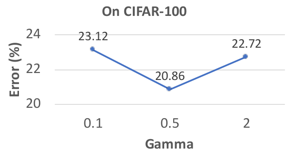
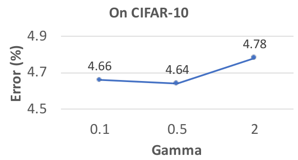
Figure 4 shows how classification errors change as increases. As can be seen, on both CIFAR-100 and CIFAR-10, when increases from 0.1 to 0.5, the error decreases. However, further increasing renders the error to increase. From the tester’s perspective, explores a tradeoff between difficulty and meaningfulness of the tests. Increasing encourages the tester to create tests that are more meaningful. Tests with more meaningfulness can more reliably evaluate the learner. However, if is too large, the tests are biased to be more meaningful and less difficult. Lacking enough difficulty, the tests may not be compelling enough to drive the learner for improvement. Such a tradeoff effect is observed in the results on CIFAR-10 as well.
Figure 5 shows how classification errors change as increases. As can be seen, on both CIFAR-100 and CIFAR-10, when increases from 0.1 to 0.5, the error decreases. However, further increasing renders the error to increase. Under a larger , the created test plays a larger role in training the tester to perform the target task. This implicitly encourages the test creator to generate tests that are more meaningful. However, if is too large, the training is dominated by the created test which incurs the following risk: if the test is not meaningful, it will result in a poor-quality data-encoder which further degrades the quality of test creation.
3.3 Summary
In this section, we apply Skillearn to formalize a skill in human learning – learning by passing tests (LPT) and use it for neural architecture search. In LPT, a tester model creates a sequence of tests with growing levels of difficulty. A learner model continuously improves its learning ability by striving to pass these increasingly more-challenging tests. The tester learns to select hard validation examples rendering the learner to make large prediction errors and the learner refines its model to rectify these prediction errors. Our framework achieves significant improvement in neural architecture search on CIFAR-100, CIFAR-10, and ImageNet.
4 Case Study II: Interleaving Learning
In this section, we instantiate our general Skillearn framework to formalize another human learning technique – interleaving learning, and apply it to improve machine learning. Interleaving learning is a learning technique where a learner interleaves the studies of multiple topics: study topic for a while, then switch to , subsequently to ; then switch back to , and so on, forming a pattern of . Interleaving learning is in contrast to blocked learning, which studies one topic very thoroughly before moving to another topic. Compared with blocked learning, interleaving learning increases long-term retention and improves ability to transfer learned knowledge.
We are interested in investigating whether the interleaving strategy is helpful for training machine learning models. We instantiate the Skillearn framework to an interleaving learning (IL) framework. We assume there are learning tasks, each performed by a learner model. Each learner has a data encoder and a task-specific head. The data encoders of all learners share the same architecture, but may have different weight parameters. The learners perform rounds of interleaving learning with the following order:
| (27) |
where denotes that the -th learner performs learning. In the first round, we first learn , then learn , and so on. At the end of the first round, is learned. Then we move to the second round, which starts with learning , then learns , and so on. This pattern repeats until the rounds of learning are finished. Between two consecutive learners , the encoder weights of the latter learner are encouraged to be close to the optimally learned encoder weights of the former learner .
4.1 Method
| Notation | Meaning |
|---|---|
| Number of learners | |
| Number of rounds | |
| Training dataset of the -th learner | |
| Validation dataset of the -th learner | |
| Encoder architecture shared by all learners | |
| Weight parameters in the data encoder of the -th learner in the -th round | |
| Weight parameters in the task-specific head of the -th learner in the -th round | |
| The optimal encoder weights of the -th learner in the -th round | |
| The optimal weight parameters of the task-specific head in the -th learner in the -th round | |
| Tradeoff parameter |
In this section, we present the details of the interleaving learning framework. There are learners. Each learner learns to perform a task. These tasks could be the same, e.g., image classification on CIFAR-10; or different, e.g., image classification on CIFAR-10, image classification on ImageNet (Deng et al. 2009), object detection on MS-COCO (Lin et al. 2014), etc. Each learner has a training dataset and a validation dataset . Each learner has a data encoder and a task-specific head performing the target task. For example, if the task is image classification, the data encoder could be a convolutional neural network extracting visual features of the input images and the task-specific head could be a multi-layer perceptron which takes the visual features of an image extracted by the data encoder as input and predicts the class label of this image. We assume the architecture of the data encoder in each learner is learnable. The data encoders of all learners share the same architecture, but their weight parameters could be different in different learners. The architectures of task-specific heads are manually designed by humans and they could be different in different learners. The learners perform rounds of interleaving learning with the following order:
| (28) |
where denotes that the -th learner performs learning. In the first round, we first learn , then learn , and so on. At the end of the first round, is learned. Then we move to the second round, which starts with learning , then learns , and so on. This pattern repeats until the rounds of learning are finished. Between two consecutive learners , the weight parameters of the latter learner are encouraged to be close to the optimally learned encoder weights of the former learner . For each learner, the architecture of its encoder remains the same across all rounds; the weights of the encoder and head can be different in different rounds.
Each learner has the following learnable parameter sets: 1) architecture of the encoder; 2) in each round , the learner’s encoder has a set of weight parameters specific to this round; 3) in each round , the learner’s task-specific head has a set of weight parameters specific to this round. The encoders of all learners share the same architecture and this architecture remains the same in different rounds. The encoders of different learners have different weight parameters. The weight parameters of a learner’s encoder are different in different rounds. Different learners have different task-specific heads in terms of both architectures and weight parameters. In the interleaving process, the learning of the -th learner is assisted by the -th learner. Specifically, during learning, the encoder weights of the -th learner are encouraged to be close to the optimal encoder weights of the -th learner. This is achieved by minimizing an interactive function: .
| Active learners | The first learner |
|---|---|
| Active learnable parameters | Weights of the data encoder and weights of the task-specific head in the first learner |
| Supporting learnable parameters | Encoder architecture shared by all learners |
| Active training datasets | Training dataset of the first learner |
| Active auxiliary datasets | – |
| Training loss | The first learner trains the weights of its data encoder and the weights of its task-specific head on its training dataset: . |
| Interaction function | – |
| Optimization problem |
There are learning stages: in each of the rounds, each of the learners is learned in a stage. In the very first learning stage, the first learner in the first round is learned. It trains the weight parameters of its data encoder and the weight parameters of its task-specific head on its training dataset. In this learning stage (Table 13), the active learner is the first learner. The active learnable parameters are the weight parameters of the data encoder and the weight parameters of the task-specific head in the first learner in the first round. The supporting learnable parameters include the encoder architecture shared by all learners. The active training dataset is the training data of the first learner. There is no auxiliary dataset. The training loss is the target-task’s loss defined on the training dataset of the first learner: . There is no interaction function. The optimization problem is:
| (29) |
In this optimization problem, is not learned. After learning, the optimal head is discarded. The optimal encoder weights are a function of since the training loss is a function of and is a function of the training loss. is passed to the next learning stage to help with the learning of the second learner.
In any other learning stage (Table 14), e.g., the -th stage where the learner is and the round of interleaving is , the active learner is the learner . The active learnable parameters include weights of the data encoder and weights of the task-specific head in the -th learner in the -th round. The supporting learnable parameters are the encoder architecture shared by all learners. The active training dataset is the training dataset of the -th learner. There is no active auxiliary dataset. The training loss is the target-task’s loss defined on the training dataset of the -th learner: . The interaction function encourages the encoder weights at this stage to be close to the optimal encoder weights learned in the previous stage. The optimization problem is:
| (30) |
where is a tradeoff parameter.
The optimal encoder weights are a function of the encoder architecture. The encoder architecture is not updated at this learning stage. In the round of 1 to , the optimal heads are discarded after learning. In the round of , the optimal heads are retained and will be used in the validation stage.
| Active learners | The -th learner |
|---|---|
| Active learnable parameters | Weights of the data encoder and weights of the task-specific head in the -th learner |
| Supporting learnable parameters | Encoder architecture shared by all learners |
| Active training datasets | Training dataset of the -th learner |
| Active auxiliary datasets | – |
| Training loss | The -th learner trains the weights of its data encoder and the weights of its task-specific head on its training dataset: |
| Interaction function | The learner encourages its encoder weights to be close to the optimal encoder weights learned in the stage: |
| Optimization problem |
| Active learners | All learners |
|---|---|
| Remaining learnable parameters | Encoder’s architecture of all learners |
| Validation datasets | Validation datasets of all learners |
| Active auxiliary datasets | – |
| Validation loss | The sum of every learner’s validation loss on its validation dataset: |
| Interaction function | – |
| Optimization problem |
In the validation stage (Table 15), the active learners are all learners. The remaining learnable parameters are the encoder architecture shared by all learners. The validation datasets are the validation datasets of all learners. There is no active auxiliary dataset. The validation loss is the sum of every learner’s validation loss calculated using the optimal encoder weights and head weights learned in the final round: . There is no interaction function. The optimization problem is:
| (31) |
Putting all these pieces together, we instantiate the Skillearn framework to an interleaving learning framework, as shown in Eq.(32). From bottom to top, the learners perform rounds of interleaving learning. Learners in adjacent learning stages are coupled via the interaction function. The architecture is not updated in the learning stages. It is learned by minimizing the validation loss. Table 16 summarizes the key elements of interleaving learning under the Skillearn terminology.
| (32) |
| Skillearn | Interleaving Learning |
|---|---|
| Learners | learners |
| Learnable parameters | 1) Encoder architecture shared by all learners; 2) In each round, each learner has weight parameters for the data encoder and weight parameters for the task-specific head. |
| Interaction function | The encoder weights at learning stage are encouraged to be close to the optimal encoder weights at stage : . |
| Learning stages | 1) In the first learning stage (the first learner in the first round), the learner trains the weights of its data encoder and the weights of its task-specific head on its training dataset: ; 2) In other learning stages, the learner trains the weights of its data encoder and the weights of its task-specific head on its training dataset where the encoder weights are encouraged to be close to the optimal encoder weights trained in the previous stage: . |
| Validation stage | Each learner validates its optimal data encoder and task-specific head learned in the last round on its validation dataset. |
| Datasets | Each learner has a training dataset and a validation dataset. |
4.2 Optimization Algorithm
In this section, we develop an optimization algorithm for interleaving learning by instantiating the general optimization framework of Skillearn in Section 2.3. For each optimization problem in a learning stage, we approximate the optimal solution by one-step gradient descent update of the optimization variable :
| (33) |
For , the approximation is:
| (34) |
For , the approximation is:
| (35) |
where is the approximation of . Note that are calculated recursively, where is a function of , is a function of , and so on. When and , . For , the approximation is:
| (36) |
In the validation stage, we plug in the approximations of and into the validation loss function, calculate the gradient of the approximated objective w.r.t the encoder architecture , then update via:
| (37) |
The update steps from Eq.(34) to Eq.(37) until convergence. The entire algorithm is summarized in Algorithm 3.
4.3 Experiments
We apply interleaving learning for neural architecture search in image classification tasks. Two tasks are interleaved: image classification on CIFAR-10 and image classification on CIFAR-100. We search the shared architecture of data encoders in these two tasks.
| Method | Error(%) | Param(M) | Cost |
|---|---|---|---|
| *ResNet (He et al. 2016a) | 22.10 | 1.7 | - |
| DenseNet (Huang et al. 2017) | 17.18 | 25.6 | - |
| *PNAS (Liu et al. 2018a) | 19.53 | 3.2 | 150 |
| ENAS (Pham et al. 2018) | 19.43 | 4.6 | 0.5 |
| AmoebaNet (Real et al. 2019) | 18.93 | 3.1 | 3150 |
| †DARTS-1st (Liu et al. 2019) | 20.520.31 | 1.8 | 0.4 |
| GDAS (Dong and Yang 2019) | 18.38 | 3.4 | 0.2 |
| R-DARTS (Zela et al. 2020) | 18.010.26 | - | 1.6 |
| DARTS- (Chu et al. 2020a) | 17.510.25 | 3.3 | 0.4 |
| †DARTS- (Chu et al. 2020a) | 18.970.16 | 3.1 | 0.4 |
| ΔDARTS+ (Liang et al. 2019a) | 17.110.43 | 3.8 | 0.2 |
| DropNAS (Hong et al. 2020) | 16.39 | 4.4 | 0.7 |
| *DARTS-2nd (Liu et al. 2019) | 20.580.44 | 1.8 | 1.5 |
| JL(DARTS2nd) | 18.920.17 | 2.4 | 3.1 |
| IL(DARTS2nd) (ours) | 17.120.08 | 2.6 | 3.2 |
| *P-DARTS (Chen et al. 2019) | 17.49 | 3.6 | 0.3 |
| JL(PDARTS) | 17.670.31 | 3.5 | 0.6 |
| IL(PDARTS) (ours) | 16.140.17 | 3.6 | 0.6 |
| PC-DARTS (Xu et al. 2020) | 17.960.15 | 3.9 | 0.1 |
| JL(PCDARTS) | 18.110.27 | 3.9 | 0.2 |
| IL(PCDARTS) (ours) | 17.830.14 | 3.8 | 0.3 |
| Method | Error(%) | Param(M) | Cost |
|---|---|---|---|
| *DenseNet (Huang et al. 2017) | 3.46 | 25.6 | - |
| *HierEvol (Liu et al. 2018b) | 3.750.12 | 15.7 | 300 |
| NAONet-WS (Luo et al. 2018) | 3.53 | 3.1 | 0.4 |
| PNAS (Liu et al. 2018a) | 3.410.09 | 3.2 | 225 |
| ENAS (Pham et al. 2018) | 2.89 | 4.6 | 0.5 |
| NASNet-A (Zoph et al. 2018) | 2.65 | 3.3 | 1800 |
| AmoebaNet-B (Real et al. 2019) | 2.550.05 | 2.8 | 3150 |
| *DARTS-1st (Liu et al. 2019) | 3.000.14 | 3.3 | 0.4 |
| R-DARTS (Zela et al. 2020) | 2.950.21 | - | 1.6 |
| GDAS (Dong and Yang 2019) | 2.93 | 3.4 | 0.2 |
| SNAS (Xie et al. 2019) | 2.85 | 2.8 | 1.5 |
| ΔDARTS+ (Liang et al. 2019a) | 2.830.05 | 3.7 | 0.4 |
| BayesNAS (Zhou et al. 2019) | 2.810.04 | 3.4 | 0.2 |
| MergeNAS (Wang et al. 2020) | 2.730.02 | 2.9 | 0.2 |
| NoisyDARTS (Chu et al. 2020b) | 2.700.23 | 3.3 | 0.4 |
| ASAP (Noy et al. 2020) | 2.680.11 | 2.5 | 0.2 |
| SDARTS (Chen and Hsieh 2020) | 2.610.02 | 3.3 | 1.3 |
| DARTS- (Chu et al. 2020a) | 2.590.08 | 3.5 | 0.4 |
| †DARTS- (Chu et al. 2020a) | 2.970.04 | 3.3 | 0.4 |
| DropNAS (Hong et al. 2020) | 2.580.14 | 4.1 | 0.6 |
| FairDARTS (Chu et al. 2019) | 2.54 | 3.3 | 0.4 |
| DrNAS (Chen et al. 2020) | 2.540.03 | 4.0 | 0.4 |
| *DARTS2nd (Liu et al. 2019) | 2.760.09 | 3.3 | 1.5 |
| JL(DARTS2nd) | 2.910.12 | 2.4 | 3.1 |
| IL(DARTS2nd) (ours) | 2.620.04 | 2.6 | 3.2 |
| *PC-DARTS (Xu et al. 2020) | 2.570.07 | 3.6 | 0.1 |
| JL(PCDARTS) | 2.630.05 | 3.9 | 0.2 |
| IL(PCDARTS) (ours) | 2.550.11 | 3.8 | 0.3 |
| *P-DARTS (Chen et al. 2019) | 2.50 | 3.4 | 0.3 |
| JL(PDARTS) | 2.630.12 | 3.5 | 0.6 |
| IL(PDARTS) (ours) | 2.510.10 | 3.6 | 0.6 |
| Method | Top-1 | Top-5 | Param | Cost |
| Error (%) | Error (%) | (M) | (GPU days) | |
| *Inception-v1 (Szegedy et al. 2015) | 30.2 | 10.1 | 6.6 | - |
| MobileNet (Howard et al. 2017) | 29.4 | 10.5 | 4.2 | - |
| ShuffleNet 2 (v1) (Zhang et al. 2018) | 26.4 | 10.2 | 5.4 | - |
| ShuffleNet 2 (v2) (Ma et al. 2018) | 25.1 | 7.6 | 7.4 | - |
| *NASNet-A (Zoph et al. 2018) | 26.0 | 8.4 | 5.3 | 1800 |
| PNAS (Liu et al. 2018a) | 25.8 | 8.1 | 5.1 | 225 |
| MnasNet-92 (Tan et al. 2019) | 25.2 | 8.0 | 4.4 | 1667 |
| AmoebaNet-C (Real et al. 2019) | 24.3 | 7.6 | 6.4 | 3150 |
| *SNAS (Xie et al. 2019) | 27.3 | 9.2 | 4.3 | 1.5 |
| BayesNAS (Zhou et al. 2019) | 26.5 | 8.9 | 3.9 | 0.2 |
| PARSEC (Casale et al. 2019) | 26.0 | 8.4 | 5.6 | 1.0 |
| GDAS (Dong and Yang 2019) | 26.0 | 8.5 | 5.3 | 0.2 |
| DSNAS (Hu et al. 2020) | 25.7 | 8.1 | - | - |
| SDARTS-ADV (Chen and Hsieh 2020) | 25.2 | 7.8 | 5.4 | 1.3 |
| PC-DARTS (Xu et al. 2020) | 25.1 | 7.8 | 5.3 | 0.1 |
| ProxylessNAS (Cai et al. 2019) | 24.9 | 7.5 | 7.1 | 8.3 |
| FairDARTS (CIFAR-10) (Chu et al. 2019) | 24.9 | 7.5 | 4.8 | 0.4 |
| FairDARTS (ImageNet) (Chu et al. 2019) | 24.4 | 7.4 | 4.3 | 3.0 |
| DrNAS (Chen et al. 2020) | 24.2 | 7.3 | 5.2 | 3.9 |
| DARTS+ (ImageNet) (Liang et al. 2019a) | 23.9 | 7.4 | 5.1 | 6.8 |
| DARTS- (Chu et al. 2020a) | 23.8 | 7.0 | 4.9 | 4.5 |
| DARTS+ (CIFAR-100) (Liang et al. 2019a) | 23.7 | 7.2 | 5.1 | 0.2 |
| *DARTS2nd(CIFAR10) (Liu et al. 2019) | 26.7 | 8.7 | 4.7 | 1.5 |
| JL(DARTS2nd,CIFAR10/100) | 26.4 | 8.5 | 3.5 | 3.1 |
| IL(DARTS2nd,CIFAR10/100) (ours) | 25.5 | 8.0 | 3.8 | 3.2 |
| *PDARTS(CIFAR10) (Chen et al. 2019) | 24.4 | 7.4 | 4.9 | 0.3 |
| PDARTS(CIFAR100) (Chen et al. 2019) | 24.7 | 7.5 | 5.1 | 0.3 |
| JL(PDARTS,CIFAR10/100) | 25.0 | 7.9 | 5.1 | 0.6 |
| IL(PDARTS,CIFAR10/100) (ours) | 24.1 | 7.1 | 5.3 | 0.6 |
4.3.1 Experimental Settings
We follow the experimental protocol in (Liu et al. 2019). Each experiment consists of a search phrase and an evaluation phrase. In the search phrase, an optimal architecture cell is searched. In the evaluation phrase, the searched cell is copied multiple times and these copies are stacked into a larger network. The larger network is trained from scratch. Each experiment was repeated 10 times with different random initialization.
In interleaving learning, we perform two tasks: image classification on CIFAR-100 and image classification on CIFAR-10, using two classification models and . CIFAR-10 contains 10 classes and CIFAR-100 contains 100 classes. For CIFAR-10 and CIFAR-100, each of them is split into a 25K training set, a 25K validation set, and a 10K test set. The training and validation set of CIFAR-100 is used as and respectively; the training and validation set of CIFAR-10 is used as and respectively. For the architecture search space of the feature extractors, we experimented with the search spaces of DARTS (Liu et al. 2019), P-DARTS (Chen et al. 2019), and PC-DARTS (Xu et al. 2020). These search spaces are composed of and (dilated) separable convolutions, max pooling, average pooling, zero, and identity. For the CIFAR-100 classification head, we set it to a 100-way linear classifier. For the CIFAR-10 classification head, we set it to a 10-way linear classifier.
During architecture search, we perform two rounds of learning, with an order of CIFAR-100, CIFAR-10, CIFAR-100, CIFAR-10. The tradeoff parameter in interleaving learning was set to 100. The network of the feature extractor is a stack of 8 cells. Each cell has 7 nodes. We set the initial channel number to 16. We optimized the architecture variables using Adam (Kingma and Ba 2014). The learning rate was set to 3e-5 for IL-DARTS, 6e-4 for IL-P-DARTS, and 3e-3 for IL-PC-DARTS. The weight decay was set to 1e-3. We optimized the network weights using SGD. The initial learning rate was set to 0.025 for IL-DARTS and IL-P-DARTS and 0.1 for IL-PC-DARTS. The batch size was set to 64 for IL-DARTS and IL-P-DARTS and 256 for IL-PC-DARTS. The epoch number was set to 50 for IL-DARTS and IL-PC-DARTS and 25 for IL-P-DARTS. Weight decay was set to 3e-4 and momentum was set to 0.9. Cosine decay scheduler was used for scheduling the learning rate. The search was performed on a single Teslav100 GPU.
During architecture evaluation, the searched cell in interleaving learning is evaluated on CIFAR-10 and CIFAR-100 independently. For either dataset, 20 copies of the searched cell are composed into a larger network as the feature extractor, which is trained on the combination of training and validation sets and tested on the test set. The initial channel number was set to 36. We trained the network for 600 epochs, with a mini-batch size of 96 for IL-DARTS and 64 for IL-P-DARTS and IL-PC-DARTS. The evaluation on CIFAR-10 and CIFAR-100 was performed on a single Tesla v100 GPU. Given the architecture searched on CIFAR10/100, we also evaluate it on ImageNet. Specifically, 14 copies of the searched cell are composed into a larger network as the feature extractor, which is trained on 1.2M training images in ImageNet and tested on 50K testing images. We set the initial channel number to 48. The number of epochs was set to 250. The batch size was set to 1024. The training on ImageNet was performed on Tesla v100 GPUs.
4.3.2 Experimental Results
Table 17 and Table 18 shows the results on CIFAR-100 and CIFAR-10 respectively, including classification errors on the test set, number of model parameters, and search cost (GPU days). As can be seen, applying interleaving learning (IL) to DARTS-2nd, P-DARTS, and PC-DARTS significantly reduces the errors of these baselines approaches. For example, on CIFAR-100, applying IL to DARTS-2nd reduces the error from 20.58% to 17.12% and applying IL to P-DARTS reduces the error from 17.49% to 16.14%. As another example, on CIFAR-10, applying IL to DARTS-2nd reduces the error from 2.76% to 2.62%. These results show that interleaving learning can help to search better architectures. With interleaving learning, the search task on CIFAR-100 and CIAFR-10 can mutually benefit each other. The feature extractor trained on CIFAR-100 is used to initialize the feature extractor for CIFAR-10. Since is trained on CIFAR-100, it is better than random weights. Therefore, using to initialize is better than random initialization. Likewise, the trained on CIFAR-10 is used to initialize in the next round of training, which is better than random initialization. These two feature extractors mutually help each other to improve in the interleaving process. In baseline approaches, such a mechanism is missing. Therefore, interleaving learning achieves better performance than the baselines.
One may wonder whether the performance gain of interleaving learning is due to more data (CIFAR100+CIFAR10) is used. To investigate this, we compare interleaving learning with a joint learning (JL) baseline with the following formulation:
| (38) |
where denotes the architecture of the feature extractors; and denote the feature extractor weights and classification head of model (for CIFAR-100); and denote the feature extractor weights and classification head of model (for CIFAR-10). In the inner optimization problem (on the constraint), we train , , , and by minimizing the training losses defined of both datasets, with the architecture fixed. In the outer optimization problem, we update the architecture by minimizing the validation losses of both datasets. In this formulation, the architecture is learned using both datasets. Table 17 and Table 18 show the results of this joint learning (JL) formulation. As can be seen, our IL method outperforms JL. For example, on CIFAR-100, when applied to DARTS-2nd, the error of IL is 17.12% while that of JL is 18.92%; when applied to P-DARTS, the error of IL is 16.14% while that of JL is 17.67%. As another example, on CIFAR-10, when applied to DARTS-2nd, the error of IL is 2.62% while that of JL is 2.91%. These results show that the performance gain of interleaving learning comes from the interleaving mechanism rather than due to more data is used. In the JL formulation, the weights of feature extractors of model and are trained independently. In contrast, in IL, the weights of feature extractors of model and mutually help each other to improve via pretraining in the interleaving process. Therefore, IL achieves better performance than JL. It is worth noting that while IL achieves better performance than baselines, it does not substantially increase parameter number or search cost.
Table 19 shows the results on ImageNet, including top-1 and top-5 errors, number of model parameters, and search cost (GPU days). From this table, we make the following observations. First, applying IL to DARTS and P-DARTS reduces the errors of these two baselines. For example, applying IL to DARTS-2nd reduces the top-1 error from 26.7% to 25.5% and reduces the top-5 error from 8.7% to 8.0%. This further demonstrates the effectiveness of IL in searching better architectures by encouraging two models to mutually help each other in the interleaving process. Second, IL achieves better performance than JL. For example, applied to DARTS-2nd, the top-1 and top-5 errors of IL are lower than those in JL. This further shows that the performance gain of IL comes from the interleaving process rather than leveraging more data. Third, while achieving better performance, IL does not substantially increase parameter number or search cost.
4.4 Summary
In this section, we apply Skillearn to formalize the interleaving learning (IL) skill of humans. In IL, a set of models collaboratively learn a data encoder in an interleaving fashion: the encoder is trained by model 1 for a while, then passed to model 2 for further training, then model 3, and so on; after trained by all models, the encoder returns back to model 1 and is trained again, then moving to model 2, 3, etc. This process repeats for multiple rounds. Via interleaving, different models transfer their learned knowledge to each other to better represent data and avoid being stuck in bad local optimums. Experiments of neural architecture search on CIFAR-100 and CIFAR-10 demonstrate the effectiveness of interleaving learning.
4.5 Related Works
4.5.1 Neural Architecture Search
Neural architecture search (NAS) has achieved remarkable progress recently, which aims at searching for the optimal architecture of neural networks to achieve the best predictive performance. In general, there are three paradigms of methods in NAS: reinforcement learning (RL) approaches (Zoph and Le 2017; Pham et al. 2018; Zoph et al. 2018), evolutionary learning approaches (Liu et al. 2018b; Real et al. 2019), and differentiable approaches (Cai et al. 2019; Liu et al. 2019; Xie et al. 2019). In RL-based approaches, a policy is learned to iteratively generate new architectures by maximizing a reward which is the accuracy on the validation set. Evolutionary learning approaches represent the architectures as individuals in a population. Individuals with high fitness scores (validation accuracy) have the privilege to generate offspring, which replaces individuals with low fitness scores. Differentiable approaches adopt a network pruning strategy. On top of an over-parameterized network, the weights of connections between nodes are learned using gradient descent. Then weights close to zero are pruned later on. There have been many efforts devoted to improving differentiable NAS methods. In P-DARTS (Chen et al. 2019), the depth of searched architectures is allowed to grow progressively during the training process. Search space approximation and regularization approaches are developed to reduce computational overheads and improve search stability. PC-DARTS (Xu et al. 2020) reduces the redundancy in exploring the search space by sampling a small portion of a super network. Operation search is performed in a subset of channels with the held-out part bypassed in a shortcut. Our proposed LCT framework can be applied to any differentiable NAS methods.
4.5.2 Adversarial Learning
Our proposed LPT involves a min-max optimization problem, which is analogous to that in adversarial learning. Adversarial learning (Goodfellow et al. 2014a) has been widely applied to 1) data generation (Goodfellow et al. 2014a; Yu et al. 2017) where a discriminator tries to distinguish between generated images and real images and a generator is trained to generate realistic data by making such a discrimination difficult to achieve; 2) domain adaptation (Ganin and Lempitsky 2015) where a discriminator tries to differentiate between source images and target images while the feature learner learns representations which make such a discrimination unachievable; 3) adversarial attack and defence (Goodfellow et al. 2014b) where an attacker adds small perturbations to the input data to alter the prediction outcome and the defender trains the model in a way that the prediction outcome remains the same given perturbed inputs. Different from these existing works, in our work, a tester aims to create harder tests to “fail” the learner while the learner learns to “pass” however hard tests created by the tester. Shu et al. 2020 proposed to use an adversarial examiner to identify the weakness of a trained model. Our work differs from this one in that we progressively re-train a learner model based on how it performs on the tests dynamically created by a tester model while the learner model in (Shu et al. 2020) is fixed and not affected by the examination results.
5 Conclusions
In this paper, we develop a general framework called Skillearn to formalize humans’ learning skills into machine-executable learning skills and leverage them to train better machine learning models. Our framework can flexibly formulate many learning skills of humans, by mapping from learners, learnable parameters, interaction functions, learning stages, etc. in Skillearn to their counterparts in human learning. The formulated machine-executable learning skills can be applied to improve any ML model. In two case studies, we apply Skillearn to formalize two learning skills of humans – learning by passing tests (LPT) and interleaving learning (IL). In LPT, a tester model dynamically creates tests with increasing levels of difficulty to evaluate a testee model; the testee continuously improves its architecture by passing however difficult tests created by the tester. In IL, a set of models collaboratively learn a data encoder in an interleaving fashion: the encoder is trained by model 1 for a while, then passed to model 2 for further training, then model 3, and so on; after trained by all models, the encoder returns back to model 1 and is trained again, then moving to model 2, 3, etc. This process repeats for multiple rounds. Experiments on various datasets demonstrate that ML models trained by these two learning skills achieve significantly better performance.
References
- Cai et al. (2019) Han Cai, Ligeng Zhu, and Song Han. Proxylessnas: Direct neural architecture search on target task and hardware. In ICLR, 2019.
- Casale et al. (2019) Francesco Paolo Casale, Jonathan Gordon, and Nicoló Fusi. Probabilistic neural architecture search. CoRR, abs/1902.05116, 2019.
- Chen and Hsieh (2020) Xiangning Chen and Cho-Jui Hsieh. Stabilizing differentiable architecture search via perturbation-based regularization. CoRR, abs/2002.05283, 2020.
- Chen et al. (2020) Xiangning Chen, Ruochen Wang, Minhao Cheng, Xiaocheng Tang, and Cho-Jui Hsieh. Drnas: Dirichlet neural architecture search. CoRR, abs/2006.10355, 2020.
- Chen et al. (2019) Xin Chen, Lingxi Xie, Jun Wu, and Qi Tian. Progressive differentiable architecture search: Bridging the depth gap between search and evaluation. In ICCV, 2019.
- Chu et al. (2019) Xiangxiang Chu, Tianbao Zhou, Bo Zhang, and Jixiang Li. Fair DARTS: eliminating unfair advantages in differentiable architecture search. CoRR, abs/1911.12126, 2019.
- Chu et al. (2020a) Xiangxiang Chu, Xiaoxing Wang, Bo Zhang, Shun Lu, Xiaolin Wei, and Junchi Yan. DARTS-: robustly stepping out of performance collapse without indicators. CoRR, abs/2009.01027, 2020a.
- Chu et al. (2020b) Xiangxiang Chu, Bo Zhang, and Xudong Li. Noisy differentiable architecture search. CoRR, abs/2005.03566, 2020b.
- Deng et al. (2009) Jia Deng, Wei Dong, Richard Socher, Li-Jia Li, Kai Li, and Li Fei-Fei. Imagenet: A large-scale hierarchical image database. In 2009 IEEE conference on computer vision and pattern recognition, pages 248–255. Ieee, 2009.
- Dong and Yang (2019) Xuanyi Dong and Yi Yang. Searching for a robust neural architecture in four GPU hours. In CVPR, 2019.
- Ganin and Lempitsky (2015) Yaroslav Ganin and Victor Lempitsky. Unsupervised domain adaptation by backpropagation. In International Conference on Machine Learning, pages 1180–1189, 2015.
- Goodfellow et al. (2014a) Ian Goodfellow, Jean Pouget-Abadie, Mehdi Mirza, Bing Xu, David Warde-Farley, Sherjil Ozair, Aaron Courville, and Yoshua Bengio. Generative adversarial nets. In Advances in neural information processing systems, pages 2672–2680, 2014a.
- Goodfellow et al. (2014b) Ian J Goodfellow, Jonathon Shlens, and Christian Szegedy. Explaining and harnessing adversarial examples. arXiv preprint arXiv:1412.6572, 2014b.
- He et al. (2016a) Kaiming He, Xiangyu Zhang, Shaoqing Ren, and Jian Sun. Deep residual learning for image recognition. In CVPR, 2016a.
- He et al. (2016b) Kaiming He, Xiangyu Zhang, Shaoqing Ren, and Jian Sun. Deep residual learning for image recognition. In CVPR, 2016b.
- He et al. (2019) Kaiming He, Haoqi Fan, Yuxin Wu, Saining Xie, and Ross Girshick. Momentum contrast for unsupervised visual representation learning. arXiv preprint arXiv:1911.05722, 2019.
- Hong et al. (2020) Weijun Hong, Guilin Li, Weinan Zhang, Ruiming Tang, Yunhe Wang, Zhenguo Li, and Yong Yu. Dropnas: Grouped operation dropout for differentiable architecture search. In IJCAI, 2020.
- Howard et al. (2017) Andrew G. Howard, Menglong Zhu, Bo Chen, Dmitry Kalenichenko, Weijun Wang, Tobias Weyand, Marco Andreetto, and Hartwig Adam. Mobilenets: Efficient convolutional neural networks for mobile vision applications. CoRR, abs/1704.04861, 2017.
- Hu et al. (2020) Shoukang Hu, Sirui Xie, Hehui Zheng, Chunxiao Liu, Jianping Shi, Xunying Liu, and Dahua Lin. DSNAS: direct neural architecture search without parameter retraining. In CVPR, 2020.
- Huang et al. (2017) Gao Huang, Zhuang Liu, Laurens van der Maaten, and Kilian Q. Weinberger. Densely connected convolutional networks. In CVPR, 2017.
- Kingma and Ba (2014) Diederik Kingma and Jimmy Ba. Adam: A method for stochastic optimization. International Conference on Learning Representations, 12 2014.
- Liang et al. (2019a) Hanwen Liang, Shifeng Zhang, Jiacheng Sun, Xingqiu He, Weiran Huang, Kechen Zhuang, and Zhenguo Li. DARTS+: improved differentiable architecture search with early stopping. CoRR, abs/1909.06035, 2019a.
- Liang et al. (2019b) Hanwen Liang, Shifeng Zhang, Jiacheng Sun, Xingqiu He, Weiran Huang, Kechen Zhuang, and Zhenguo Li. Darts+: Improved differentiable architecture search with early stopping. arXiv preprint arXiv:1909.06035, 2019b.
- Lin et al. (2014) Tsung-Yi Lin, Michael Maire, Serge Belongie, James Hays, Pietro Perona, Deva Ramanan, Piotr Dollár, and C Lawrence Zitnick. Microsoft coco: Common objects in context. In ECCV, 2014.
- Liu et al. (2018a) Chenxi Liu, Barret Zoph, Maxim Neumann, Jonathon Shlens, Wei Hua, Li-Jia Li, Li Fei-Fei, Alan L. Yuille, Jonathan Huang, and Kevin Murphy. Progressive neural architecture search. In ECCV, 2018a.
- Liu et al. (2018b) Hanxiao Liu, Karen Simonyan, Oriol Vinyals, Chrisantha Fernando, and Koray Kavukcuoglu. Hierarchical representations for efficient architecture search. In ICLR, 2018b.
- Liu et al. (2019) Hanxiao Liu, Karen Simonyan, and Yiming Yang. DARTS: differentiable architecture search. In ICLR, 2019.
- Luo et al. (2018) Renqian Luo, Fei Tian, Tao Qin, Enhong Chen, and Tie-Yan Liu. Neural architecture optimization. In NeurIPS, 2018.
- Ma et al. (2018) Ningning Ma, Xiangyu Zhang, Hai-Tao Zheng, and Jian Sun. Shufflenet V2: practical guidelines for efficient CNN architecture design. In ECCV, 2018.
- Noy et al. (2020) Asaf Noy, Niv Nayman, Tal Ridnik, Nadav Zamir, Sivan Doveh, Itamar Friedman, Raja Giryes, and Lihi Zelnik. ASAP: architecture search, anneal and prune. In AISTATS, 2020.
- Pham et al. (2018) Hieu Pham, Melody Y. Guan, Barret Zoph, Quoc V. Le, and Jeff Dean. Efficient neural architecture search via parameter sharing. In ICML, 2018.
- Real et al. (2019) Esteban Real, Alok Aggarwal, Yanping Huang, and Quoc V Le. Regularized evolution for image classifier architecture search. In Proceedings of the aaai conference on artificial intelligence, volume 33, pages 4780–4789, 2019.
- Shu et al. (2020) Michelle Shu, Chenxi Liu, Weichao Qiu, and Alan Yuille. Identifying model weakness with adversarial examiner. In Proceedings of the AAAI Conference on Artificial Intelligence, volume 34, pages 11998–12006, 2020.
- Szegedy et al. (2015) Christian Szegedy, Wei Liu, Yangqing Jia, Pierre Sermanet, Scott Reed, Dragomir Anguelov, Dumitru Erhan, Vincent Vanhoucke, and Andrew Rabinovich. Going deeper with convolutions. In CVPR, 2015.
- Tan et al. (2019) Mingxing Tan, Bo Chen, Ruoming Pang, Vijay Vasudevan, Mark Sandler, Andrew Howard, and Quoc V. Le. Mnasnet: Platform-aware neural architecture search for mobile. In CVPR, 2019.
- Wang et al. (2020) Xiaoxing Wang, Chao Xue, Junchi Yan, Xiaokang Yang, Yonggang Hu, and Kewei Sun. Mergenas: Merge operations into one for differentiable architecture search. In IJCAI, 2020.
- Xie et al. (2019) Sirui Xie, Hehui Zheng, Chunxiao Liu, and Liang Lin. SNAS: stochastic neural architecture search. In ICLR, 2019.
- Xu et al. (2020) Yuhui Xu, Lingxi Xie, Xiaopeng Zhang, Xin Chen, Guo-Jun Qi, Qi Tian, and Hongkai Xiong. PC-DARTS: partial channel connections for memory-efficient architecture search. In ICLR, 2020.
- Yu et al. (2017) Lantao Yu, Weinan Zhang, Jun Wang, and Yong Yu. Seqgan: Sequence generative adversarial nets with policy gradient. In AAAI, 2017.
- Zela et al. (2020) Arber Zela, Thomas Elsken, Tonmoy Saikia, Yassine Marrakchi, Thomas Brox, and Frank Hutter. Understanding and robustifying differentiable architecture search. In ICLR, 2020.
- Zhang et al. (2018) Xiangyu Zhang, Xinyu Zhou, Mengxiao Lin, and Jian Sun. Shufflenet: An extremely efficient convolutional neural network for mobile devices. In CVPR, 2018.
- Zhou et al. (2019) Hongpeng Zhou, Minghao Yang, Jun Wang, and Wei Pan. Bayesnas: A bayesian approach for neural architecture search. In ICML, 2019.
- Zoph and Le (2017) Barret Zoph and Quoc V. Le. Neural architecture search with reinforcement learning. In ICLR, 2017.
- Zoph et al. (2018) Barret Zoph, Vijay Vasudevan, Jonathon Shlens, and Quoc V Le. Learning transferable architectures for scalable image recognition. In CVPR, 2018.