Nonlinearity accelerates the thermalization of the quartic FPUT model with stochastic baths
Abstract
We investigate the equilibration process of the strongly coupled quartic Fermi-Pasta-Ulam-Tsingou (FPUT) model by adding Langevin baths to the ends of the chain. The time evolution of the system is investigated by means of extensive numerical simulations and shown to match the results expected from equilibrium statistical mechanics in the time-asymptotic limit. Upon increasing the nonlinear coupling, the thermalization of the energy spectrum displays an increasing asymmetry in favour of small-scale, high-frequency modes, which relax significantly faster than the large-scale, low-frequency ones. The global equilibration time is found to scale linearly with system size and shown to exhibit a power-law decay with the strength of the nonlinearity and temperature. Nonlinear interaction adds to energy distribution among modes, thus speeding up the thermalization process.
Keywords: Fermi-Pasta-Ulam-Tsingou, Equilibration time, Canonical ensemble, Langevin heat baths
1 Introduction
Thermalization in the Fermi-Pasta-Ulam-Tsingou (FPUT) model has attracted much attention since the original formulation of the problem [1, 2, 3]. In the weak coupling regime the system reaches equipartition on a timescale which depends as a power-law [4, 5, 6] on the energy density. In this work, we take a different approach by studying the equilibration process ranging from the weak to the strong coupling regime. In particular, we explore the steady-state dynamics and the relaxation to steady-state of the quartic FPUT attaching stochastic Langevin baths to both ends of the chain. A detailed study of the nonlinear model in equilibrium conditions was performed in [7] by realizing the canonical setting in a textbook manner, considering a small part of the microcanonical system. We show that our description using Langevin baths proves to be a successful framework to simulate both equilibrium and non-equilibrium properties of the nonlinear model in a canonical setting. We find by numerical simulations of the stochastic equations that increasing the nonlinear coupling accelerates the approach to equilibrium. Even at high nonlinearity equilibrium is surprisingly characterized by quasi-equipartition of linear energy among Fourier modes and relaxation to equilibrium is faster for high-frequency modes. We derive analytically a compact representation of the equilibrium properties of the model, introducing a dimensionless scaling variable with temperature of the baths and coupling strength . The expressions obtained from the canonical partition function for equilibrium quantities, such as internal energy and nonlinear energy, are in satisfactory agreement with the numerical results of the stochastic model. The equilibration time is shown to be linear in the system-size for a sufficiently large number of oscillators and is probed as a function of coupling (temperature) at different temperatures (couplings). We find that both dependencies are well-fitted by a decaying power-law with exponent across four decades in temperature.
2 The model
We consider the following extension to the quartic FPUT with particles given by the Langevin equations [8]
| (1) |
where the baths at the left and right edge () have the same temperature
| (2) |

Fixed boundary conditions were imposed such that . Initially, the position and momenta are plain for all sites, and . For reasons of simplicity, the mass and the spring constant of the harmonic interaction are set to unity, i.e. and . Having a physical realization of our system in mind [9, 10], we couple stochastic motion only to the edges of the chain. The Langevin approach for the baths is a special case of the general Markovian evolution of the baths where the reservoirs are not affected by the system at all. The particular choice of the baths provides a physical implementation of the thermostats compared with more efficient schemes like Nosé-Hoover baths [11, 12] which have been applied to determine probability distributions for canonical momenta [13]. The model without nonlinearity () coupled to Langevin baths is known to thermalize, i. e. all particles have equal kinetic energy as time goes to infinity [14, 15].
3 Numerical implementation
We have integrated the equations of motion using a standard fourth order Runge-Kutta scheme (RK4) for the deterministic part and a simple first order Euler–Maruyama method for the stochastic term [16]. Other integration schemes (e.g. Velocity-Verlet), have also been considered for the deterministic part, which proved to be slower at a comparable order of accuracy. Setting the dissipation to unity ( fixed for the rest of the paper), a stepsize proved to be stable and sufficiently accurate for the purpose of this paper. Considering the deterministic part separately (), the largest observed deviation from energy conservation using the RK4 scheme, was of the order of , for the case of sites and strong nonlinearity . For the full stochastic system, equipartition was reached numerically and the fluctuation-dissipation theorem was satisfied within less then 1 % for the longest simulation times (5000 timesteps). Ensemble-averaging and time-averaging were implemented simultaneously for every quantity under inspection. In equations:
| (3) |
with being a measured quantity for a single Wiener-process realization. Unless explicitly mentioned otherwise, we will refer from now on to every quantity in the text as the averaged one. A window of and runs are used for the statistics. Numerical errors appear due the choice of the timestep which affects predominantly the integration of the stochastic part, due to the low-order Euler-Mayurama scheme (time-integration is numerically more costly than ensemble-averaging since the latter can be run in parallel across independent tasks). We have checked the validity of our results by doubling the timestep, size of the ensemble and of the time-averaging window for the time-average, thus confirming satisfactory convergence of the stochastic simulations. Higher order schemes for the stochastic part might improve the efficiency of the code and will be considered in the future for longer time simulations.


4 Time-evolution of the normal modes
The kinetic energy of a single site defines a temperature distribution in real space . For the linear Langevin chain (recovered by setting ) all oscillators equilibrate to the temperature of the baths, i. e. [14, 17]. We will show that this holds also for the nonlinear case. It is useful to introduce the normal modes of the harmonic system [18]
| (4) |
Their frequencies are and the linear energy is given by . The total energy stored in the linear motion of the modes is . The probability to find the system in mode is adopted according to [5, 19, 20]
| (5) |
If the nonlinearity is weak the total energy is well-approximated by the linear energy in the modes, i. e. . This is not true anymore for the strong coupling regime. Nevertheless, (5) defines the probability distribution of the normal modes at every value of the coupling, and is properly normalized by . Excluding an anharmonic term from the definition gives us a clear perspective on the modification of the spectrum when the coupling is changed. We observe that the nonlinearity has an impact on the time evolution of the spectrum .
Snapshots of temperature profiles and the distribution of modes for different coupling strengths are shown at different points during their evolution in figure 2 and 3. For the latest time in our simulation, the system approaches a homogeneous temperature in real space and a flat spectrum in mode space, regardless of the coupling strength. Comparing distributions/temperature profiles for different coupling strengths at the early points in the evolution, the nonlinearity accelerates the thermalization process. For the linear case (), modes around are fastest excited at early stages in the evolution. In comparison with the real space evolution, the exterior sites and attached to the baths are early excited. Low- and high-oscillating Fourier modes at the ends of the spectrum reach equipartition latest and nearly at the same time. Ramping up , an asymmetry in the spectrum is observed, as high-oscillating modes are quicker to reach equipartition than the low ones. At (figure 2 c)), the first snapshot in the evolution (black curve) displays a spectrum which is almost flat for modes and steeply declines for low-oscillating modes. The high-oscillating modes approach equilibrium on the same time scale as the fastest relaxed modes whereas low modes trail behind.
5 Thermodynamics from the stochastic model
Next, we derive analytic expressions for the internal energy, and the nonlinear and harmonic part of the energy in equilibrium. They are required to validate the corresponding time-asymptotic quantities in the simulation of the stochastic quartic FPUT. The partition function for the system reads
| (6) |
with momenta and as well as . Singling out the kinetic term we make the coordinate transformation [7]
| (7) |
The variables and are not real coordinates but parameters due to the fixed boundaries. The Jacobian of the transformation is invertible and has determinant equal to the identity. The partition function is transformed to
| (8) |
displaying the same contribution of every variable . The prefactor is a relict of the transformation and does not depend on the coordinates due to the fixed boundary conditions. The integral of the quartic exponential is found in terms of modified Bessel functions of the second kind . The partition function becomes
| (9) |

This is equivalent to the result given in [7] by the relation of the parabolic cylinder functions and the Bessel functions , upon changing from fixed to periodic boundary conditions.
The internal energy is related to the partition function by . We obtain
| (10) |
where we have definded the ratio of the Bessel functions
| (11) |
Again, the result is equivalent to [7]. Dividing in (10) by , the internal energy has a dimensionless scale
| (12) |
The coupling plays by the found relation for the role of an inverse nonlinear temperature scale. It is also worth investigating the harmonic part and nonlinear part of the energy
| (13) | |||||
| (14) |
where is the Hamiltonian of the quartic FPUT. The change of variables (7) and rewriting by parameter differentiation yields
| (15) | |||||
| (16) |
The result can again be given in dimensionless form
| (17) |
Observe that for infinitely strong coupling , so the asymptotics is given by
| (18) |
The asymptotic (and maximum) ratio of nonlinear energy and internal energy settles at . The following ratio yields the contribution of nonlinear coupling to potential energy
| (19) |
It assumes values on the unit interval, i.e. (purely linear) and (purely nonlinear), and thus provides a good measure to separate strong from weak coupling which we define by
| (20) |
We have simulated the linear case up to values (at ), covering both weak and strong coupling regime. The stochastic implementation of the canonical ensemble of the quartic FPUT shows quantitative agreement with the values of internal, linear and nonlinear energy expected from equilibrium statistical mechanics (see figure 4).
6 Equilibration time


Having assessed the equilibrium properties of the system, next we utilize the stochastic
model to numerically investigate the dependence of the relaxation to steady-state
on the system size, temperature and nonlinearity.
We define the equilibration time as the minimum time for which
the total energy reaches the equilibrium energy
(10) and stays around it within fluctuations
of the order of a small fraction of .
Numerically, it is convenient to take a window
(illustrated in figure 5 b)).
For a given temperature and coupling , we find that the equilibration
time depends linearly on the system size, provided is large enough,
see figure 6.
We have fixed (strong coupling) and plotted
as a function of for various temperatures, finding good agreement with the
following fit (the numerical values of the parameters are given in Appendix A)
| (21) |
Besides being directly suggested by visual inspection of the numerical data, this
fit also responds to a simple physical interpretation.
Indeed, is associated to single-body relaxation time, while
is the increment of due to the insertion of a single
extra-node in the lattice chain. For large , a linear scaling is clearly observed, with
coefficient depending on the temperature, but not on the coupling strength.
The main outcome of this analysis is the linear dependence of on .
Figure 7 reports
the equilibration time as a function of the nonlinearity .
For a given temperature, the curves for different are equidistantly spaced,
e.g.
indicating that depends only weakly on the nonlinear coupling.
For the case of a few sites , temperature (at fixed )
has no effect on the equilibration time, as seen from the fact that all curves
in the figure 6 merge into a single one
for ).


The linear dependence of on the system size is the main result of the work. We have added a cubic nonlinearity to the quartic FPUT model (1) and performed simulations to study for fixed and (not shown in this paper). The linear relationship is still valid in this case, as long as the cubic nonlinearity is sufficiently weak to act as perturbation to the quartic model, namely as long as the potential displays a single minimum.
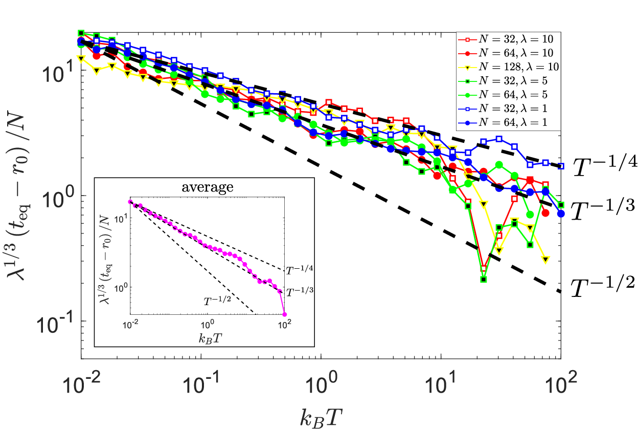
Next, we analyse the relaxation time as a function of temperature (see figure 8). The equilibration time decays weakly over a large range of simulated bath temperatures, and appears to be satisfactorly fitted by a power-law decay of the form:
| (22) |
Fitting more generally , the exponent is
found for different couplings and system sizes (see
A). The first parameter decays
weakly with and increases linearly with , as
the two curves for and in each subfigure
8 a)
- c) are almost equidistantly spaced. The second parameter
is a sublinear function of and numerically
almost independent on , since the curves in figure
8 a)
- c) (different , fixed ) have the same value
for the largest bath temperature. We relate the parameters
in (21)
and (22)
in the large limit: the parameter takes
numerically values similar to the case of the single-body
relaxation time in our simulations at large .
By expanding
(21) in
, we identify the term with , thereby
deducing .
At last, we investigate the effect of the coupling on
the equilibration time. From the spectral time evolution
(see figure 2), we have already observed that
equilibration is accelerated by nonlinearity.
As in the temperature-dependent study, depends weakly on ,
a power-law with a small exponent
| (23) |
We have again assumed first a general dependence like
, and concluded
from our data that (see A).
The time-asymptotic value does not significantly depend on , and increases with
, assuming numerically comparable values like and .
Again, we can indentify them in the large -limit and relate to
and , to give the leading contribution to the equilibration time in temperature
(there might be also a contribution from ).
It follows that and scale like .
The power-laws (22)
and (23) can be motivated by dimensional analysis. The quantity
| (24) |
has the dimension of a inverse time. This suggests that if the equilibration time depends like a power-law on , then it should also depend like a power-law on with the same exponent, and vice versa. Like in thermal equilibrium, plays the role of an inverse temperature. The other time-scales in the problem are the inverse dissipation constant, multiplied by the mass and the harmonic frequency . The simulations provide strong evidence for a behavior of the form , see figure 9, hence the nonlinear frequency enters like .
7 Discussion and conclusion
We have implemented the quartic FPUT model and succesfully reproduced
the equilibrium canonical ensemble using Langevin baths.
The equilibrium energy of our numerical approach agrees with the internal
energy expected from the canonical ensemble (cf. figure 4).
By an exact integration of the partition function of the nonlinear chain, we have been able to
recover non-perturbative results from statistical mechanics, covering
both weak and strong coupling regimes.
Numerical integration of the stochastic differential equations matched the expression of the
internal, nonlinear energy and harmonic energy from statistical mechanics in the time-asymptotic limit.
It was found that the mentioned components of the equilibrium energy of the quartic FPUT, normalized
to the thermal energy in a linear chain, depend only on the product of
temperature and coupling via the dimensionless scaling ,
i. e. .
By the found scaling in , we can make a proportionality argument: consider
the potential of a single bond of
the quartic FPUT and a change in coupling .
The internal energy of the bond remains exactly the same if we cool down the
bond by , regardless of the interaction strength, temperature
of the baths and also system size. At equilibrium, all bonds feel the bath as
if it was adjacent to them.
The amount of nonlinearity is likewise only a function of , providing a
closed formula (19) to distinguish quantitatively
between the strong and weak coupling regimes.
Attaching the nonlinear system in the framework of Langevin baths puts us
in the position to investigate the time evolution of the FPUT during the
thermalization process.
It is found that the nonlinearity accelerates equipartition, although not to a dramatic extent.
This becomes clear from comparing the classic FPUT with the harmonic chain
in terms of energy distribution.
In the harmonic chain, energy is kept only in the intially excited mode, whereas
in the FPUT case, energy is distributed among all modes
(provided at least one even and odd modes are initially excited in the quartic FPUT).
When thermal baths are attached to the nonlinear FPUT, energy equipartition
is reached through the Langevin terms under the presence of nonlinearity, while in the
linear chain, this is obtained solely by the action of the Langevin terms.
Nonlinear interaction adds to energy distribution
among modes, thus speeding up the thermalization process.
This happens selectively in different regions of the spectrum.
Energy is faster channeled to the high modes as the coupling is amplified.
The equipartition time is a function of system size, temperature and coupling strength.
For large enough (), it increases linearly with the system size, with
the slope dependent on temperature but not on the coupling strength.
The relaxation time is increased by increasing the temperature of the baths
and displays a power law behavior with exponent .
Increasing the coupling leads to quicker equilibration, following
again power-law dependence, with approximately the same exponent.
In a future work, the faster distribution of energy, favoring high-oscillating modes, should
be investigated by considering the transient solution of the mode equations.
It would also be interesting to investigate the effect of dimensionality on the scaling of
the equilibration time with system size.
We hope that the stochastic implementation of the canonical ensemble presented in this paper
can prove useful to study equilibrium and non-equilibrium properties of
similar nonlinear models, such as the Toda chain.
Acknowledgments
This work is part of MUR-PRIN2017 project ”Coarse-grained description for non- equilibrium systems and transport phenomena (CO-NEST)” No. 201798CZL whose partial financial support is acknowledged. One of the authors (SS) acknowledges funding from the European Research Council under the Horizon 2020 Programme Grant Agreement n. 739964 (”COPMAT”). HS was financially supported by the ERASMUS program and the Physics Advanced program of the Elite Network of Bavaria (University of Regensburg, Germany), and is grateful for the hospitality of the Scuola Normale Superiore.
Appendix A Fitting parameters
| 0.1 | 1 | 10 | |
|---|---|---|---|
| 8.4 | 7.5 | 5.8 |
00 , , , ,
References
References
- [1] Fermi E, Pasta P and Ulam S 1955 Studies of nonlinear problems Tech. rep. Los Alamos Scientific Lab., N. Mex.
- [2] Gallavotti G 2007 The Fermi-Pasta-Ulam problem: a status report vol 728 (Berlin, Heidelberg: Springer Verlag)
- [3] Berman G P and Izrailev F M The Fermi–Pasta–Ulam problem: Fifty years of progress 2005 Chaos 15 015104
- [4] Benettin G, Christodoulidi H and Ponno A The Fermi-Pasta-Ulam Problem and Its Underlying Integrable Dynamics 2013 J. Stat. Phys. 152 195–212
- [5] Onorato M, Vozella L, Proment D and Lvov Y V Route to thermalization in the -Fermi–Pasta–Ulam system 2015 Proceedings of the National Academy of Sciences 112 4208–4213
- [6] Lvov Y V and Onorato M Double Scaling in the Relaxation Time in the -Fermi-Pasta-Ulam-Tsingou Model 2018 Phys. Rev. Lett. 120 144301
- [7] Livi R, Pettini M, Ruffo S and Vulpiani A Chaotic behavior in nonlinear Hamiltonian systems and equilibrium statistical mechanics 1987 J. Stat. Phys. 48 539–559
- [8] Lepri S, Livi R and Politi A Thermal conduction in classical low-dimensional lattices 2003 Physics Reports 377 1–80
- [9] Experimental realization of Fermi-Pasta-Ulam-Tsingou recurrence in a long-haul optical fiber transmission system 2019 Scientific Reports 9 1–11
- [10] Pierangeli D, Flammini M and Zhang L e a 2019 Fermi-Pasta-Ulam-Tsingou Recurrence in Spatial Optical Dynamics 2019 Conference on Lasers and Electro-Optics Europe & European Quantum Electronics Conference (CLEO/Europe-EQEC) pp 1–1
- [11] Nosé S A unified formulation of the constant temperature molecular dynamics methods 1984 The Journal of Chemical Physics 81 511–519
- [12] Hoover W G Canonical dynamics: Equilibrium phase-space distributions 1985 Phys. Rev. A 31 1695–1697
- [13] Demirel M C and Sayar M Statistical mechanics of Fermi-Pasta-Ulam chains with the canonical ensemble 1997 Phys. Rev. E 55 3727–3730
- [14] Rieder Z, Lebowitz J L and Lieb E Properties of a Harmonic Crystal in a Stationary Nonequilibrium State 1967 J. Math. Phys 8 1073–1078
- [15] Kim S Temperature profile and equipartition law in a Langevin harmonic chain 2017 J. Korean Phys. Soc. 71 264–268
- [16] Press W H, Teukolsky S A, Vetterling W T and Flannery B P 2007 Numerical recipes (Cambridge university press)
- [17] Nakazawa H On the Lattice Thermal Conduction 1970 Progress of Theoretical Physics Supplement 45 231–262
- [18] Ford J The Fermi-Pasta-Ulam problem: Paradox turns discovery 1992 Physics Reports 213 271–310
- [19] Livi R, Pettini M, Ruffo S, Sparpaglione M and Vulpiani A Equipartition threshold in nonlinear large Hamiltonian systems: The Fermi-Pasta-Ulam model 1985 Phys. Rev. A 31(2) 1039–1045
- [20] Pistone L, Chibbaro S, D Bustamante M, V Lvov Y and Onorato M Universal route to thermalization in weakly-nonlinear one-dimensional chains 2019 Mathematics in Engineering 1 672–698