Structured Index Coding Problem
and Multi-access Coded Caching

Index coding is a fundamental problem in network information theory [2] which consists of a central server with a collection of messages, communicating with a set of users over a broadcast channel. Each user has prior knowledge of a subset of the messages, referred to as side-information, and is interested in recovering another subset of the messages. The goal of the index coding problem (ICP) is to minimize the server transmission size while satisfying all the user requests. While the problem in general remains open, several bounds are known based on min rank [3], local chromatic number [4], local partial clique cover [5] and maximum acyclic induced subgraph (MAIS)[6]. There has been work on characterizing the optimal transmission rate for specific classes of ICPs such as the uniprior ICP [7], single unicast index coding problem (SUICP) with symmetric neighboring and consecutive (SUICP-SNC) side-information [8, 9], SUICP with symmetric consecutive interference (SUICP-SCI) [10] and the ICP with interlinked cycle structure [11]. An ICP is said to be symmetric [8], if the relative positions of side-information and interference users are the same for all the users. In this work, we focus on a new class of structured ICPs which are formed by the union of several symmetric ICPs and are motivated by the multi-access coded caching problem (MACC) [12].

ICP also has close relations to several other active research topics, including network coding [13], distributed storage [14], distributed computing [15], and coded caching [16]. The coded caching problem was introduced in [17], which pioneered an information-theoretic view of the classical caching problem, and helps in reducing the network congestion by offloading the data traffic from peak to off-peak hours. The setup in [17] (Ali-Niesen setup) consists of a central server with $N$ files, each of size 1 unit, communicating over an error-free broadcast link with $K$ users each with a cache of size $M$ units. There are two phases in the system. The first phase is the placement phase, in which the content related to the files is stored in the caches. The second phase is the delivery phase, in which each user requests a file from the central server, and these requests are served by the central server with the help of the caches. The aim is to minimize the central server transmission while ensuring that each user can recover its requested file using the server’s transmission message and the cache content user has access to. [17] proposed a (uncoded²² 2 In the uncoded placement policy, we are allowed to split the files into parts and store the individual file parts, but coding across the file parts is not allowed while storing in the caches.) placement and (coded) delivery policy, which is order-wise optimal up to a constant factor of 12 with respect to the information-theoretic lower bound. Following this, the coded caching problem has attracted a lot of attention in the information theory community. Several works focus on improving the gap between the achievable rates and the lower bounds, see for example [16] for an extensive survey. In fact, [18, 19] showed that the policy proposed in [17] is exactly optimal under the restriction of uncoded placement. In particular, [19] exploited the connection between the coded caching and the index coding problems to prove the exact optimality.

A generalization of the Ali-Niesen setup is the multi-access coded caching (MACC) problem introduced in [12], where each user is connected to $L$ consecutive caches with a cyclic wrap-around, see Section VI for the detailed description of the problem setup. [12] proposed a (uncoded) placement and (coded) delivery policy and showed that the multiplicative gap between their achievable rate and the information-theoretic lower bound is bounded by $c\cdot L$, for some constant $c$. Following this, [20, 21, 22, 23] focus on improving the achievable rate and deriving the order-optimal bound. [20, 21, 22, 23] primarily use the uncoded placement policies and coded delivery policies.

In the second part of this paper, we establish a connection between the MACC problem to the class of structured symmetric ICPs studied in the first part, and use the results derived to establish new bounds on the optimal rate-memory trade-off of the caching problem. If the placement policy and the request pattern are fixed, then a coded caching problem is equivalent to solving an ICP. In our work, we use the same uncoded placement policy proposed in [20] and then use our ICP results in the delivery policy to derive the new bounds on the optimal rate-memory trade-off. We analytically show that our achievable rate can be better than the achievable rates in [12, 20, 23]. Furthermore, we also show via examples and numerical evaluations that there exist system parameter regimes where our achievable rate can be better than those proposed in [21, 22].

Recently, the MACC problem has also been studied in [24, 25, 26, 27]. In particular, [24, 25] focus on the MACC with linear sub-packetization. The works [26, 27] focus on a MACC problem with a slightly altered topology based on cross-resolvable designs. [26, 27] consider a new metric rate-per-user and showed that the schemes from cross-resolvable designs perform better under this new metric than the schemes in [17, 22].

Our contributions in this paper are summarized below:

1. 1.

   We define a new class of structured ICPs which are formed by the union of several symmetric ICPs. We derive upper and lower bounds on the optimal transmission rate for this class and show that they differ by at most a multiplicative factor of 2.

2. 2.

   We derive the exact optimal transmission rate of some special symmetric ICPs.

3. 3.

   We apply our ICP results to derive a new bound on the achievable rate of the MACC problem and show that our achievable rate can be better than the achievable rates in [12, 20, 21, 22, 23] using examples and numerical evaluations.

4. 4.

   For the MACC problem with access degree $L\geq K/2$, we show that our proposed achievable rate is at most a factor 5/4 away from the optimal rate under the restriction of uncoded placement. This improves the previously best known multiplicative gap of 2 [20].

The rest of the paper is organized as follows: Sections II and III define some useful notations and describe the ICP setting studied in this paper. Sections IV and V include some ICP preliminaries and present the main results respectively. Section VI describes the MACC setting and presents the improved upper bound on the optimal rate. Numerical results are given in Section VII and the summary of our work and future possible extensions are given in VIII. All the proofs are relegated to Appendix.

• •

  $[n]=\{1,2,3,...,n\}$

• •

  For some given³³ 3 In our manuscript, $K$ is the number of users in the index coding problem / multi-access coded caching problem. integer $K$ such that $K\geq m,n$,

  $\displaystyle[m:n]=\begin{cases}\{m,m+1,...,n\}&\text{ if }m\leq n\\ \{m,m+1,...,K,1,2,...,n\}&\text{ if }m>n\end{cases}$

• •

  $\displaystyle<m>_{n}=\begin{cases}m\ (\mathrm{mod}\ n)&\text{ if }m\ (\mathrm{mod}\ n)\neq 0\\ n&\text{ if }m\ (\mathrm{mod}\ n)=0\end{cases}$

• •

  $|S|-$ size of file / subfile / set $S$

• •

  ${F}_{i,\mathcal{S}}$ denotes parts of File $i$ exclusively available to users with index in set $\mathcal{S}$

• •

  $len(\mathbf{v})$ denotes the number of components of the vector $\mathbf{v}$

• •

  $\mathbf{\widehat{a}}$ denotes the maximum value amongst the components of the vector $\mathbf{a}$

An index coding problem (ICP) consists of $N$ files $\mathcal{X}=\{x_{1},x_{2},...,x_{N}\}$, each of size 1 unit ($=F$ bits⁴⁴ 4 We assume that the file size $F$ is sufficiently large.) at a central server and a set of $K$ users $\mathcal{U}=\{U_{1},U_{2},...,U_{K}\}$. Each user $U_{k}=(\mathcal{W}_{k},\mathcal{K}_{k})$ wants a subset of files $\mathcal{W}_{k}\subseteq\mathcal{X}$, and we call it the want-set of $U_{k}$. Each user $U_{k}$ knows another subset of files $\mathcal{K}_{k}\subseteq\mathcal{W}_{k}^{c}$, and we call it the known-set or side-information of $U_{k}$. The remaining subset of files $(\mathcal{W}_{k}\cup\mathcal{K}_{k})^{c}$, i.e., the files which are neither requested nor available, are called the interference-set of User $k$. The central server transmits a message such that each user $k$ recovers its want-set $\mathcal{W}_{k}$ using its known-set $\mathcal{K}_{k}$ and the central server’s transmitted message. The goal is to minimize the server transmission size while satisfying all the user requests. The minimum transmission size required to satisfy all the user demands in an ICP, over all possible coding strategies, is called the optimal transmission rate $R^{*}$ of the ICP. An ICP is said to be a unicast index coding problem (UICP) if none of the users want the same file, i.e., $\mathcal{W}_{k_{1}}\cap\mathcal{W}_{k_{2}}=\phi$, $\forall k_{1}\neq k_{2}$ and an ICP is said to be a single unicast index coding problem (SUICP) if every user wants only one file and it is a UICP, i.e., $|\mathcal{W}_{k}|=1$, $\forall k$ and $\mathcal{W}_{k_{1}}\cap\mathcal{W}_{k_{2}}=\phi$, $\forall k_{1}\neq k_{2}$.

We refer to an ICP as an $(a_{i},a_{i-1},...,a_{1})_{L}-$ICP for some non-negative integers $a_{1},a_{2},...,a_{i}$ and a natural number $L$ such that

if $\forall k\in[K]$, User $k$

• •

  wants $x_{k}$, i.e., $\mathcal{W}_{k}=\{x_{k}\}$ and

• •

  knows

  $\displaystyle\mathcal{K}_{k}=\{x_{b}:b=<k+\sum_{j=1}^{v}a_{i+1-j}+(v-1)L+r>_{K},v\in[i-1],r\in[L]\},$

  i.e., the side-information $\mathcal{K}_{k}$ is available in $i-1$ chunks, each of which is a collection of $L$ consecutive elements and the separation/gap between the consecutive chunks is determined by $a_{i},a_{i-1},\ldots,a_{1}$. More explicitly, the side information $\mathcal{K}_{k}$ of User $k$ is given by

Note that the $(a_{i},a_{i-1},...,a_{1})_{L}-$ICP is an SUICP and $|\mathcal{K}_{k}|=(i-1)L$. In an $(a_{i},a_{i-1},...,a_{1})_{L}-$ ICP, if we arrange the files $x_{1},x_{2},...,x_{K}$ circularly in clock-wise direction, then User $k$ wants File $x_{k}$ and if we go on from $x_{k}$ in clock-wise direction, first we see $a_{i}$ interference files for User $k$, then $L$ side-information files, then $a_{i-1}$ interference files, then $L$ side-information files and so on. It ends with $a_{1}$ interference files for User $k$. See Figure 1 for an illustration.

In this paper, we focus on a union of multiple SUICPs which is defined as follows. Let there be $K$ users such that User $k$ wants $\mathcal{W}_{k}^{j}$ and knows $\mathcal{K}_{k}^{j}$ in the $j^{th}$ instance for some $j\in[i]$, $i\in\mathbb{N}$, then the union of these $i$ instances is an ICP with

• •

  want set $\mathcal{W}_{k}=\mathcal{W}^{1}_{k}\cup\mathcal{W}^{2}_{k}\cup...\cup\mathcal{W}^{i}_{k}$ and

• •

  known set $\mathcal{K}_{k}=\mathcal{K}^{1}_{k}\cup\mathcal{K}^{2}_{k}\cup...\cup\mathcal{K}^{i}_{k}$.

We assume that there are no common files involved across the instances.

In this paper, we focus on a UICP formed by the union of $i\in\mathbb{N}$ special SUICPs. We use the notation $x_{k,j}$ to represent the $j^{th}$ file requested by User $k$.

We refer to an ICP as the $\overline{(a_{i},a_{i-1},...,a_{1})}_{L}-$ICP, if it is a union of the $(a_{i},a_{i-1},...,a_{1})_{L}-$ICP, $(a_{1},a_{i},...,a_{2})_{L}-$ICP, and so on till $(a_{i-1},a_{i-2},...,a_{1},a_{i})_{L}-$ICP, i.e., an $\overline{(a_{i},a_{i-1},...,a_{1})}_{L}-$ICP is formed by the union of the $(a_{i},a_{i-1},...,a_{1})_{L}-$ICP and its $i-1$ clockwise rotations. In an $\overline{(a_{i},a_{i-1},...,a_{1})}_{L}-$ICP, $a_{j}$ is a non-negative integer $\forall j\in[i]$, $L$ is a natural number and they satisfy (1). In the $\overline{(a_{i},a_{i-1},...,a_{1})}_{L}-$ICP, $\forall k\in[K]$

• •

  want set $\mathcal{W}_{k}=\{x_{k,1},x_{k,2},...,x_{k,i}\}$, and

• •

  known set

  $\displaystyle\mathcal{K}_{k}=\{x_{b,t}:t\in[i],v\in[i-1],r\in[L],b=<k+\sum_{j=1}^{v}a_{<i+t-j>_{i}}+(v-1)L+r>_{K}\},$

  (2)

  i.e.,

  $$\mathcal{K}_{k}=\mathcal{K}^{1}_{k}\cup\mathcal{K}^{2}_{k}\cup\ldots\cup\mathcal{K}^{i}_{k},$$

  where $\mathcal{K}_{k}^{p}$ is the side-information structure of $(a_{p-1},a_{p-2}...,a_{1},a_{i},...,a_{p})_{L}-$ICP, which denotes the $(p-1)^{th}$ clock-wise rotation of ${(a_{i},a_{i-1},...,a_{1})}_{L}-$ICP, and is given by

Note that in an $\overline{(a_{i},a_{i-1},...,a_{1})}_{L}-$ICP, each user wants $i$ files and has $i(i-1)L$ files as side-information. Since $\overline{(a_{i},a_{i-1},...,a_{1})}_{L}-$ICP, $\overline{(a_{1},a_{i},...,a_{2})}_{L}-$ICP, …, $\overline{(a_{i-1},a_{i-2},...,a_{1},a_{i})}_{L}-$ICP all are equivalent, we assume without loss of generality (WLOG) $a_{i}\geq a_{j}$ $\forall j\in[i]$.

An $\overline{(a_{i},a_{i-1},...,a_{1})}_{L}-$ICP can be represented by a $K\times i$ table such that the $k^{th}$ row and $j^{th}$ column contains the $j^{th}$ file requested by User $k$. We represent a general $\overline{(a_{i},a_{i-1},...,a_{1})}_{L}-$ICP in Table 1 and the $\overline{(2,1,0)}_{2}-$ICP in Table 2. We denote the $k^{th}$ row and $j^{th}$ column’s entry as Node $(k,j)$. In these tables, $k^{th}$ row represents User $k$’s requested files. In Table 2, we highlight User 3’s requested files with red color, bold fonts and its side-information files with blue color fonts and shaded nodes. A Node $(m_{1},n_{1})$ is said to be side-information node of any Node $(m_{2},n_{2})$, if User $m_{2}$ has File $x_{m_{1},n_{1}}$ in its side-information. For example, the shaded nodes in Table 2 are side-information nodes of Node $(3,1)$. Recall that an $\overline{(a_{i},a_{i-1},...,a_{1})}_{L}-$ICP is formed by the union of the $(a_{i},a_{i-1},...,a_{1})_{L}-$ICP and its $i-1$ clockwise rotations. According to our tabular representation in Table 1, the first column corresponds to the $(a_{i},a_{i-1},...,a_{1})_{L}-$ICP, the second column corresponds to the $(a_{1},a_{i},a_{i-1},...,a_{2})_{L}-$ICP and so on till the $i^{th}$ column which corresponds to the $(a_{i-1},a_{i-2},...,a_{1},a_{i})_{L}-$ICP. In Column 1 of Table 2, User 3’s requested file is $x_{3,1}$ and it is followed by the two interference files $x_{4,1}$ and $x_{5,1}$, then two side-information files $x_{6,1}$ and $x_{7,1}$, then one interference file $x_{8,1}$, then two side-information files $x_{1,1}$ and $x_{2,1}$ and it ends with the 0 interference files. From symmetry, the same structure holds in the first column for all other users as well and thus we can conclude that the first column corresponds to $(2,1,0)_{2}-$ICP. Similarly, we can verify that the second column corresponds to $(0,2,1)_{2}-$ICP and the third column corresponds to $(1,0,2)_{2}-$ICP.

Our aim is to find the optimal broadcast rate of an $\overline{(a_{i},a_{i-1},...,a_{1})}_{L}-$ICP.

There are several upper and lower bounds [6, 4, 5, 3] available for an SUICP. We use local chromatic number and maximum acyclic induced sub-graph based bounds in our proofs and they are described below.

In an SUICP, User $j$ is said to be interfering with User $k$, if User $j$ is requesting a file from $\mathcal{K}_{k}^{c}$, i.e., User $j$’s requested file is not available at User $k$. The closed anti-outneighborhood of User $k$ is defined as the set containing User $k$ itself and all its interfering users and is denoted by $\mathcal{N}^{+}(k)$. A proper coloring scheme assigns a color to each user such that no user shares its color with any of its interfering users. For an SUICP with $m$ users, let $c:[m]\rightarrow[n]$ for some positive integer $n\leq m$ be a proper coloring scheme with $n$ colors and let $c(\mathcal{N}^{+}(k))$ denote the set of different colors assigned to the closed anti-outneighborhood of User $k$ under coloring scheme $c$. Then the local chromatic number of the ICP ($\mathcal{X}_{l}$) is defined as

In words, the local chromatic number of an ICP is defined as the maximum number of different colors that appear in any user’s closed anti-outneighborhood, minimized over all proper coloring schemes.

Lemma 1 gives an upper bound on the optimal broadcast rate of an SUICP and it follows from [4, Theorem 1]. [4] also discusses the explicit construction of server transmission schemes based on MDS codes which achieve this bound.

An SUICP with $m$ users can equivalently be represented by a side information graph $\mathcal{G}$ with $m$ nodes such that each node represents a unique user and there exists an edge from Node $k$ to Node $j$ if User $j$’s requested file belongs to Known-set $\mathcal{K}_{k}$ of User $k$.

Lemma 2 gives a lower bound on the optimal broadcast rate of an SUICP and it follows from [3, Theorem 3].

In this section, we discuss our main results related to the $\overline{(a_{i},a_{i-1},...,a_{1})}_{L}-$ICP. Let the variable $R_{u}$ be defined as

The following theorem gives an upper bound on the optimal rate of the $\overline{(a_{i},a_{i-1},...,a_{1})}_{L}-$ICP.

As mentioned in Section IV, the local chromatic number gives an upper bound on the SUICP. So, we convert a UICP with $K$ users into an SUICP with $iK$ virtual users such that each user in the UICP maps into $i$ virtual users in the SUICP, and each virtual user requests a distinct file of the original user’s requested files. The side-information at the virtual user is the same as its corresponding real user. We find an upper bound on the local chromatic number by assigning a proper coloring scheme to the virtual users. This upper bound works as an upper bound for the broadcast rate of the original problem. One naive coloring scheme is to assign a unique color to each virtual user. Note that for this coloring scheme, the number of colors assigned to the closed anti-outneighborhood of any virtual user is $iK-i(i-1)L$. This is because the total number of users is $iK$ and the size of the side-information set for any user is $i(i-1)L$. In this paper, we propose a better coloring scheme, which gives the upper bound shown in Theorem 1. The details are given in Appendix -A. Here, we discuss the coloring scheme and upper bound for the $\overline{(2,1,0)}_{2}-$ICP mentioned in Example 2. Note that for the $\overline{(2,1,0)}_{2}-$ICP, the bound corresponding to the naive coloring scheme is $iK-i(i-1)L=12$ whereas our proposed scheme gives a bound of $2(K-(i-1)L)+i-2-a_{i}=7$.

Recall that the upper bound in Theorem 1 is the minimum of $K$ and $2(K-(i-1)L)+i-2-a_{i}$. For the $\overline{(2,1,0)}_{2}-$ICP discussed in Example 2, we got the upper bound as $2(K-(i-1)L)+i-2-a_{i}$ $(<K)$. Now, we discuss the $\overline{(3,2,1)}_{2}-$ICP in Example 3, where we get $K$ $(<2(K-(i-1)L)+i-2-a_{i})$ as upper bound.

Thus far, we have discussed the achievable schemes and the upper bounds on broadcast rate for the $\overline{(a_{i},a_{i-1},...,a_{1})}_{L}$ $-$ICP. Now, we focus on the lower bound on the optimal broadcast rate of the $\overline{(a_{i},a_{i-1},...,a_{1})}_{L}$ $-$ICP and check the tightness of the bounds. The following theorem gives a lower bound on the optimal broadcast rate of the $\overline{(a_{i},a_{i-1},...,a_{1})}_{L}$ $-$ICP and its proof is given in Appendix -B.

The following corollary compares the bounds in Theorems 1 and 2, and shows that the rate achieved by our proposed scheme is always within a factor of two from the optimal.

The multi-access coded caching (MACC) problem was proposed in [12] and has been studied recently in [20, 22, 21] under the additional assumption of uncoded placement. In particular, the bounds proposed in [20] are based on establishing a mapping between the MACC problem and a class of ICPs. Along similar lines, we use the ICP results derived in the previous section to derive a new achievable rate for the MACC problem and also compare it to other achievable rates in the literature.

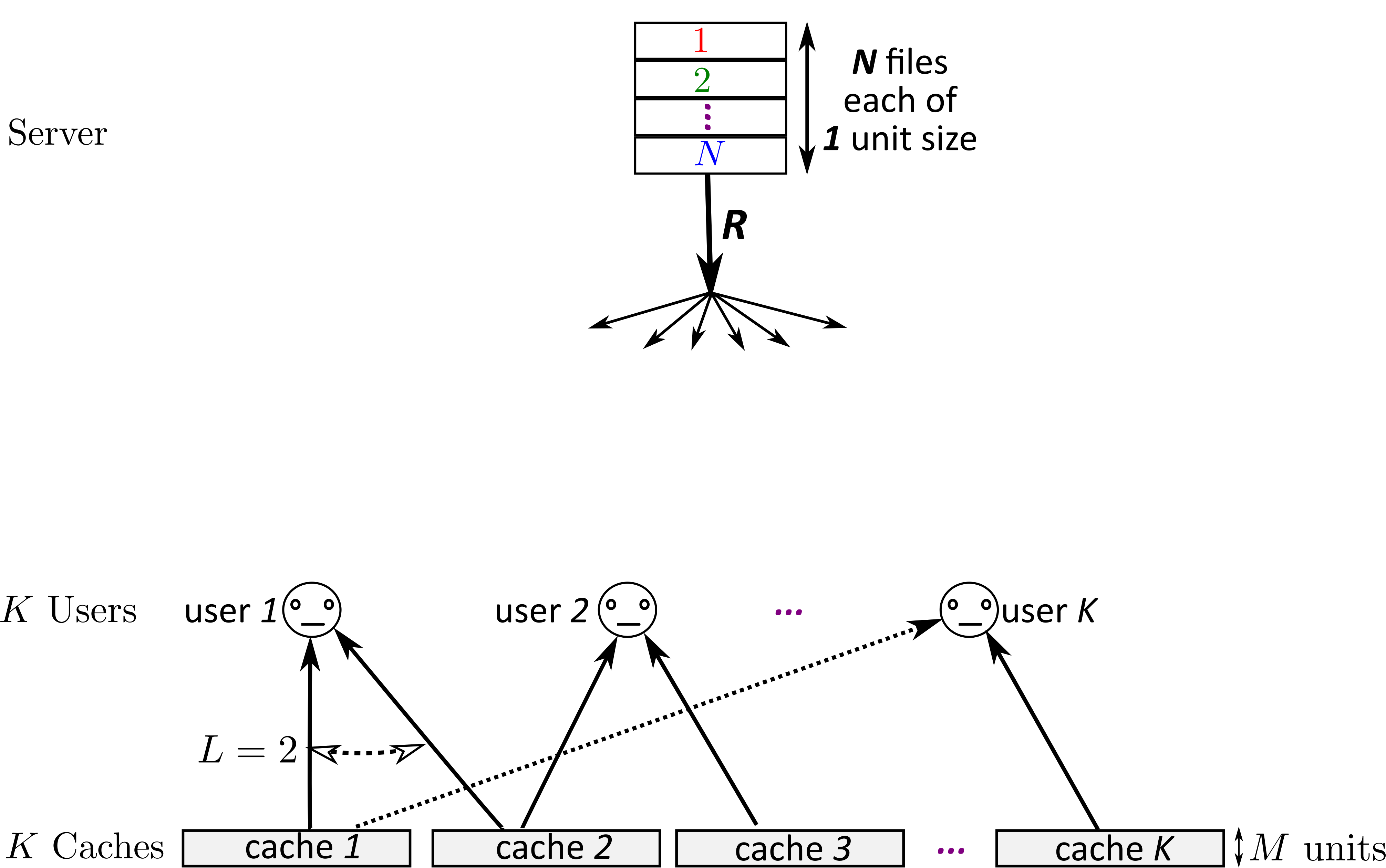
The MACC setup in [12] consists of a central server with $N$ files $\mathcal{F}_{1},\mathcal{F}_{2},...,\mathcal{F}_{N}$, each of size 1 unit. There are $K$ caches, each of size $M$ units, and $K$ users, each of which has access to $L$ consecutive caches with a cyclic wrap-around, as shown in Figure 2. The system is called as the ($N,K,L$)$-$Cache aided content delivery network (CCDN) [12]. In short, it is referred as ($N,K,L$)$-$CCDN. The system operates in two phases. The first one is the placement phase, in which we store the files according to some policy. Similar to the works in [20, 21, 22], we restrict to uncoded placement policies wherein the caches can store the individual files and parts thereof, but no coded content is cached. The second phase is the delivery phase, in which each user requests a file from the central server and we serve the user requests using a central server broadcast message and the caches’ content. Our aim is to find the central server’s optimal transmission rate ($R^{*}(M)$) for any given memory $M$ under the restriction of uncoded placement.

In our work, we use the same uncoded placement policy as the one proposed in [20] and propose a better delivery policy based on the ICP results derived in Section V. First, we consider the memory points $M$ of the form $M=wN/K$ $w\in[\lfloor K/L\rfloor]$ and derive corresponding achievable rates. The achievable rate at the intermediate points is given by memory sharing. At the extreme memory points $M=0$ units and $M=\lceil\frac{K}{L}\rceil\frac{N}{K}$ units, we can easily achieve the transmission rates $K$ units and $0$ units respectively. The details are there in [20] and also given in Appendix H-F. Now, we discuss the uncoded placement policy and delivery policy proposed for the other corner points $M=wN/K$, where $w\in[\lfloor K/L\rfloor]$.

References

- [1] K. S. Reddy and N. Karamchandani, “Structured index coding problem and multi-access coded caching,” in IEEE Information Theory Workshop (ITW), 2020, pp. 1232–1236.
- [2] Y. Birk and T. Kol, “Informed-source coding-on-demand (iscod) over broadcast channels,” in Proceedingsof the Seventeenth Annual Joint Conference of the IEEE Computer and Communications Societies (INFOCOM),.
- [3] Z. Bar-Yossef, Y. Birk, T. Jayram, and T. Kol, “Index coding with side information,” IEEE Transactions on Information Theory, vol. 57, no. 3, pp. 1479–1494, 2011.
- [4] K. Shanmugam, A. G. Dimakis, and M. Langberg, “Local graph coloring and index coding,” in IEEE International Symposium on Information Theory (ISIT), 2013, pp. 1152–1156.
- [5] A. Agarwal and A. Mazumdar, “Local partial clique covers for index coding,” arXiv preprint arXiv:1603.02366, 2016.
- [6] F. Arbabjolfaei, B. Bandemer, Y.-H. Kim, E. Şaşoğlu, and L. Wang, “On the capacity region for index coding,” in IEEE International Symposium on Information Theory (ISIT), 2013, pp. 962–966.
- [7] L. Ong, C. K. Ho, and F. Lim, “The single-uniprior index-coding problem: The single-sender case and the multi-sender extension,” IEEE Transactions on Information Theory, vol. 62, no. 6, pp. 3165–3182, 2016.
- [8] H. Maleki, V. R. Cadambe, and S. A. Jafar, “Index coding—an interference alignment perspective,” IEEE Transactions on Information Theory, vol. 60, no. 9, pp. 5402–5432, 2014.
- [9] M. B. Vaddi and B. S. Rajan, “On the minrank of symmetric and neighboring side-information index coding problems,” in IEEE Information Theory Workshop (ITW), 2019, pp. 1–5.
- [10] ——, “On the broadcast rate of index coding problems with symmetric and consecutive interference,” in 2018 International Symposium on Information Theory and Its Applications (ISITA), 2018, pp. 110–114.
- [11] C. Thapa, L. Ong, and S. J. Johnson, “Interlinked cycles for index coding: Generalizing cycles and cliques,” IEEE Transactions on Information Theory, vol. 63, no. 6, pp. 3692–3711, 2017.
- [12] J. Hachem, N. Karamchandani, and S. N. Diggavi, “Coded caching for multi-level popularity and access,” IEEE Transactions on Information Theory, vol. 63, no. 5, pp. 3108–3141, 2017.
- [13] M. Effros, S. El Rouayheb, and M. Langberg, “An equivalence between network coding and index coding,” IEEE Transactions on Information Theory, vol. 61, no. 5, pp. 2478–2487, 2015.
- [14] A. Mazumdar, “Storage capacity of repairable networks,” IEEE Transactions on Information Theory, vol. 61, no. 11, pp. 5810–5821, 2015.
- [15] S. Li, M. A. Maddah-Ali, Q. Yu, and A. S. Avestimehr, “A fundamental tradeoff between computation and communication in distributed computing,” IEEE Transactions on Information Theory, vol. 64, no. 1, pp. 109–128, 2017.
- [16] M. A. Maddah-Ali and U. Niesen, “Coding for caching: fundamental limits and practical challenges,” IEEE Communications Magazine, vol. 54, no. 8, pp. 23–29, 2016.
- [17] ——, “Fundamental limits of caching,” IEEE Transactions on Information Theory, vol. 60, no. 5, pp. 2856–2867, 2014.
- [18] Q. Yu, M. A. Maddah-Ali, and A. S. Avestimehr, “The exact rate-memory tradeoff for caching with uncoded prefetching,” IEEE Transactions on Information Theory, vol. 64, no. 2, pp. 1281–1296, 2017.
- [19] K. Wan, D. Tuninetti, and P. Piantanida, “On the optimality of uncoded cache placement,” in IEEE Information Theory Workshop (ITW), 2016, pp. 161–165.
- [20] K. S. Reddy and N. Karamchandani, “Rate-memory trade-off for multi-access coded caching with uncoded placement,” IEEE Transactions on Communications, 2020.
- [21] S. Sasi and B. S. Rajan, “An improved multi-access coded caching with uncoded placement,” arXiv preprint arXiv:2009.05377, 2020.
- [22] B. Serbetci, E. Parrinello, and P. Elia, “Multi-access coded caching: gains beyond cache-redundancy,” in IEEE Information Theory Workshop (ITW), 2019, pp. 1–5.
- [23] M. Cheng, K. Wan, D. Liang, M. Zhang, and G. Caire, “A novel transformation approach of shared-link coded caching schemes for multiaccess networks,” IEEE Transactions on Communications, 2021.
- [24] S. Sasi and B. S. Rajan, “Multi-access coded caching scheme with linear sub-packetization using pdas,” arXiv preprint arXiv:2102.06616, 2021.
- [25] A. A. Mahesh and B. S. Rajan, “A coded caching scheme with linear sub-packetization and its application to multi-access coded caching,” arXiv preprint arXiv:2009.10923, 2020.
- [26] D. Katyal, P. N. Muralidhar, and B. S. Rajan, “Multi-access coded caching schemes from cross resolvable designs,” IEEE Transactions on Communications, 2021.
- [27] P. N. Muralidhar and B. S. Rajan, “Multi-access coded caching from a new class of cross resolvable designs,” arXiv preprint arXiv:2102.00400, 2021.
- [28] R. P. Stanley, “Enumerative combinatorics volume 1 second edition,” Cambridge studies in advanced mathematics, 2011.
-A Proof of Theorem 1
We use the following lemmas to prove Theorem 1 and their proofs are relegated to Appendices H-G and H-H.
Lemma 3
In Table 1, for any User , , and ,
- •
if Node is a side-information node then Node is also a side-information node,
if Node is an interference node then Node is also an interference node.
Lemma 4
For the ICP given in Table 1, if we assign Color to nodes () , then the coloring scheme is a proper coloring scheme.
Proof:
Proof of Theorem 1: Recall that, in an ICP, each user wants files and has files as side-information. We form a table such that row and column contains file requested by User , see Table 1. We denote the row and column’s entry as Node .
Note that the ICP is a UICP with users, and each user requesting distinct files. As we did for Example 2 in Section V, we convert this UICP into an SUICP with virtual users, each one requesting a distinct file. In particular, each user in the UICP is mapped to virtual users in the SUICP, such that each virtual user requesting a distinct file of the original user’s requested files. The side-information at the virtual user is the same as its corresponding original user. In Table 1, recall that we use Node to represent the file requested by User and refer to it as the virtual user of User . The side-information for Node in the constructed SUICP is the same as the side-information for User in the original UICP. We give an upper bound for the SUICP, and it also works as a bound for the original UICP.
Recall from Section IV that for an SUICP, a proper coloring scheme assigns a color to each user such that no user shares its color with any of its interfering users. We take colors and assign Color to nodes . Note that, every color occurs in a column exactly once. Lemma 4 tells that the above coloring scheme is a proper coloring scheme.
The closed anti-outneighborhood of User is defined as the set containing User itself and all its interfering users. The local chromatic number of an ICP is defined as the maximum number of different colors that appear in the closed anti-outneighborhood of any user, minimized over all proper coloring schemes.
Consider a Node () and calculate the number of colors in closed anti-outneighborhood of it by going over column by column, i.e., we first add the first column’s colors contributing to the closed anti-outneighborhood, then we add second column’s colors contributing to the closed anti-outneighborhood, then we add third column’s colors and so on finally column’s colors. Recall that, in the first column, we assign colors with one color per node, and Node () contains side-information nodes which are not involved under the closed anti-outneighborhood. Therefore, there are colors in the first column which contribute to the closed anti-outneighborhood of Node(). Note that according to our coloring scheme, Node and Node share a common color. From Lemma 3, , if Node () is an interference node then Node ( is also an interference node. Therefore, using Lemma 3 and our coloring scheme, we can see that a color assigned to any interference node of Node (), is also assigned to an interference node of Node () in the first column and hence is already added to the set. Therefore, the nodes , don’t add any new colors to the set. According to our problem setup, amongst the remaining nodes in Column 2 given by , , there are side-information nodes. Therefore, the extra colors added from Column 1 to Column 2 are at most . Similarly, for a general , we can see that Node and Node share a common color. From Lemma 3, , if Node () is an interference node then Node ( is also an interference node. Therefore, using Lemma 3 and our coloring scheme, we can see that a color assigned to any interference node of Node (), is also assigned to an interference node of Node () in the column and hence is already added to the set. Therefore, the nodes , don’t add any new colors to the set. According to our problem setup, amongst the remaining nodes in Column given by , , there are side-information nodes. Therefore, the extra colors added from Column to Column are at most . Therefore, the total number of colors in the closed anti-outneighborhood of any Node () is less than or equal to K-(i-1)L+∑_m=1^i-1(a_m+1)= 2(K-(i-1)L)-a_i+i-2. Therefore, from Lemma 1, R^*≤X_l≤2(K-(i-1)L)+i-2-a_i.
In our coloring scheme, we are using only colors. Hence, every node contains at most colors in its closed anti-outneighborhood. Therefore, from Lemma 1, we also have R^*≤X_l≤K. This completes the proof. ∎
-B Proof of Theorem 2
As an illustration, we first discuss the ICP. Recall from Section III that the number of nodes in a ICP is given by and that the ICP can be represented by a table such that row and column contains file requested by User , see Table 9. We denote the row and column’s entry as Node . In Table 9, we also highlight User 1’s requested files with red color fonts and User 1’s side-information files with shaded cells and blue-colored fonts.
Note that the ICP is a UICP with 15 users, and each user requests 3 files. Similar to the proof of Theorem 1, we convert this UICP into an SUICP with 45 virtual users, each one requesting a distinct file. In particular, each user in the UICP is mapped to 3 virtual users in the SUICP with each virtual user requesting a distinct file from amongst the original user’s requested files. The side-information at the virtual user is the same as its corresponding original user. In Table 9, we use Node to represent the virtual user of User . The optimal broadcast rate in the two ICPs (the virtual SUICP and the original UICP) are equal. We give a lower bound for the SUICP, and it also works as a bound for the original UICP.
Recall that an SUICP with users can equivalently be represented by a side information graph with nodes such that each node represents a unique user and there exists an edge from Node to Node if User ’s requested file belongs to Known-set of User . Lemma 2 shows that the number of nodes in any acyclic induced sub-graph of the side-information graph is a lower bound on the broadcast rate of the corresponding ICP.
Now, we construct an acyclic induced sub-graph for our ICP. The idea is: first we take all nodes belonging to the same row of the ICP table, which do not contain any cycles by definition. Then, we increase the set size step by step by adding nodes row by row, which do not create cycles by their addition. To decide the nodes to be added in a row, first sort the multi-set in decreasing order. Let the sorted multi-set be , i.e., is the largest element of the multi-set and is the smallest element of the multi-set. For ICP, , Now, we shuffle the columns 2 and 3 of Table 9 so that User 1 contains interference nodes in rows 2 to in Column (see Table 9), i.e., the columns are rearranged so that the number of interference nodes in the first chunk for User 1 in each given column are in non-increasing order. Then, for each subsequent row, we start adding nodes from the left and continue till we encounter a side-information node. Note that, by rearranging the columns, the ICP doesn’t change. Now, form the acyclic induced subgraph as follows: the first set of nodes are User 1’s requested files (Row 1 nodes), then we add left nodes from each of the rows from Row to Row , then we add left nodes from each of the rows from Row to Row and finally, add nodes from each of the rows from Row to Row . First set of nodes are Row 1 nodes , and . Then, we add 3 Row 2 nodes , and . Then, we add 3 Row 3 nodes and . Then, we add 2 Row 4 nodes , and . Then, we add 1 Row 5 node and finally we add 1 Row 6 node . We highlight all these nodes with the green color in Table 9. Note that in Column , if Node is an interference node to Row 1 nodes, and none of the nodes such that are side-information to Row 1 nodes then Node is also an interference node to Row nodes . Thus, all the newly added nodes in each step are interference nodes to already existing nodes and they don’t have incoming edges from already added nodes. Therefore, the newly added nodes don’t form cycles with the already added nodes. Therefore, the acyclic induced sub-graph contains nodes , , , , , , , , , , and and from Lemma 2, . Now, we discuss the general ICP lower bound proof.
Proof of Theorem 2: An ICP can be represented by a table. The ICP above was represented in Table 9. In this tabular representation, Column represents the ICP. For User 1, in Column of the table, the number of interference nodes in the first chunk from the top are , i.e., in Column of the table, the nodes in rows 2 to are interference nodes. In the ICP, columns 1, 2 and 3 of Table 9 represent the ICP, ICP and ICP respectively. In Table 9, for User 1, the number of interference nodes in the first chunk from the top in columns 1, 2 and 3 are , and respectively. First sort the multi-set in decreasing order. Let the sorted multi-set be , i.e., is the largest element of the multi-set and is the smallest element of the multi-set. Now, we rearrange the columns such that User 1 contains interference nodes in rows 2 to in Column , i.e., the columns are rearranged so that the number of interference nodes in the first chunk for User 1 in each given column are in non-increasing order. Note that, by rearranging the columns, the ICP doesn’t change. Recall that Table 9 represents the rearranged table of Table 9. In Table 9, for User 1, the number of interference nodes in the first chunk from the top in columns 1, 2 and 3 are , and respectively, i.e., the columns are rearranged so that the number of interference nodes in the first chunk for User 1 in each given column are in non-increasing order.
Similar to the ICP, an ICP can be represented as an SUICP with virtual users, each one requesting a distinct file. Recall that an SUICP with virtual users can equivalently be represented by a side information graph with nodes such that each node represents a unique user and there exists an edge from Node to Node if User ’s requested file belongs to Known-set of User . The number of nodes in any acyclic induced sub-graph of the side-information graph is a lower bound on the broadcast rate of the corresponding ICP.
For a general ICP, we construct an acyclic induced sub-graph for our ICP from the re-arranged table as follows: First, we take all the nodes corresponding to User 1. We then continue to add all nodes from Row 2 to Row . From the definition of , we do not encounter any side-information nodes in this step. Next, for each of the rows from Row to Row , we add nodes starting from the left. We continue this until we add 1 left node from each of the rows from Row to Row . Note that, the added nodes are User 1’s nodes and all its interference nodes in the first chunk from the top across the columns. This further implies that in each step, the added nodes are interference nodes for all the nodes added previously. Therefore, while adding the new nodes, they don’t have edges from the already added nodes and thus don’t form any cycles.
The total number of nodes in the above acyclic induced sub-graph are , which is equal to From Lemma 2, ∎
-C Proof of Theorem 5
Recall that, in an ICP, each user wants files and has files as side-information. To understand the structural properties of the ICP, we form a table such that the entry in the row and column corresponds to the file requested by User , see Table 10.