A formula for membrane mediated point particle interactions on near spherical biomembranes

Charles M. Elliott Affiliation: Mathematics Institute, Zeeman Building, University of Warwick, Affiliation: Coventry, CV4 7AL. UK Email: c.m.elliott@warwick.ac.uk Affiliation: Philip J. Herbert Affiliation: Mathematics Institute, Zeeman Building, University of Warwick, Affiliation: Coventry, CV4 7AL. UK Email: p.j.herbert@warwick.ac.uk

Abstract

We consider a model of a biomembrane with attached proteins. The membrane is represented by a near spherical continuous surface and attached proteins are described as discrete rigid structures which attach to the membrane at a finite number of points. The resulting surface minimises a quadratic elastic energy (obtained by a perturbation of the Canham-Helfrich energy) subject to the point constraints which are imposed by the attachment of the proteins. We calculate the derivative of the energy with respect to protein configurations. The proteins are constrained to move tangentially by translation and by rotation in the axis normal to a reference point. Previous studies have typically restricted themselves to a nearly flat membrane and circular inclusions. A numerically accessible representation of this derivative is derived and employed in some numerical experiments.

2010 Mathematics Subject Classification: 35J35, 26B05, 65N30

Keywords: Membrane-mediated interaction, Canham-Helfrich, surface PDE, point Dirichlet constraints, mixed finite elements, domain mapping

1 Introduction

The morphology of cell membranes and a variety of functions are well-known to be regulated by the interplay between surface proteins and the curvature of the membrane. Biological membranes are composed of a lipid bilayer, this layer is believed to act like a fluid in the lateral direction and elastically in the normal direction. This means that in principle, any proteins which may be embedded into or attached to the surface of the membrane may move freely. This means that not only can the proteins influence the shape of the membrane, but also the protein interaction will be membrane mediated.

Indeed, although direct protein-protein interactions are important, [20] demonstrated that the long range interactions are predominantly membrane mediated. An overview of membrane mediated interactions is given in [3]. An assumption of symmetry of the protein inclusion allows for either analytic representation or approximation by an asymptotic expansion of the interactions [29, 37, 10, 39, 19]. Frequently the studies of these interactions were restricted to a nearly flat membrane with circular or single point inclusions. It is known that the shape of the inclusion has a significant impact on the interaction [30]. In the recent work of [35], they consider a near spherical membrane which is deformed by particles which attach along segments of an ellipsoid or hyperbolid and in [22], they consider arbitrary, sufficiently regular, particle inclusions on a flat membrane. Recent work has looked at shape formation of multiple smaller particles into larger structures [36, 21]. The article [9] considers generic elastic energies on a manifold with embedded point particles which have a given interaction potential. A variational formulation for equilibria of the surface and particle system is presented, along a discretisation. Numerical validations are given, in particular, a Helfrich problem is presented. We further note the work of [5] which considers point constraints in a Kirchoff plate, this bears a striking similarity to the biological problems of optimising the locations of constraints with respect to the an elastic membrane energy.

It is widely accepted in the literature that the near stationary state of lipid membranes are minimisers of the Canham-Helfrich energy [6, 25],

\int_{\mathcal{M}}\left(\frac{\kappa}{2}(H-c_{0})^{2}+\sigma+\kappa_{G}K\right){\rm d}\mathcal{M}.

(1.1)

Where the membrane is assumed to be thin and well modelled by a 2-dimensional surface $\mathcal{M}$ , with the quantities $\kappa>0$ , $\kappa_{G}\in\mathbb{R}$ are the bending rigidities associated to the mean and Gauss curvature respectively and $\sigma\geq 0$ is the surface tension. For the principle curvatures of $\mathcal{M}$ , $\kappa_{1},\kappa_{2}$ we take $H:=\kappa_{1}+\kappa_{2}$ to be 2 times the usual value of the mean curvature and $K:=\kappa_{1}\kappa_{2}$ the typical Gauss curvature. The value $c_{0}\in\mathbb{R}$ is the spontaneous curvature, this corresponds to a mis-match between the inner and outer layers of the membrane, for example differing lipid composition.

We make some simplifying assumptions. The first is to set $c_{0}=0$ , corresponding to a physical assumption that the mismatch between the layers is rather small. Another assumption is to neglect the Gauss curvature term. This may be justified by taking the rigidity $\kappa_{G}$ to be constant and applying the Gauss-Bonnet theorem, which states that when $\mathcal{M}$ is closed, the quantity $\int_{\mathcal{M}}K$ depends only on the Euler characteristic of $\mathcal{M}$ . As we are considering a fixed topology of near-spherical membranes, we may ignore this constant. This leads to

\int_{\mathcal{M}}\left(\frac{\kappa}{2}H^{2}+\sigma\right){\rm d}\mathcal{M}.

(1.2)

It is natural to introduce a volume constraint corresponding to the membrane being impermeable and the fluid contained within the membrane being incompressible. Indeed, without the volume constraint, it is known (1.2) is bounded below by $8\pi\kappa$ [38] and the degenerate sequence $\mathbb{S}^{2}\left(0,\frac{1}{n}\right)$ for $n\to\infty$ is a minimising sequence. Further to this, we are interested in constraining $\mathcal{M}$ to contain a set of points, this corresponds to a protein in a fixed location being attached to the membrane.

We assume that the attached proteins are rigid, that is to say they do not bend and can only move by translations or rotations. It is of clear interest to consider the force that the membrane exerts on these attached proteins. This is relevant to, say, calculate locally minimising configuration of multiple proteins via a gradient flow, to estimate statistical quantities using over-damped Langevin Dynamics [32, Section 2.2.2] or as a step for a full model for the problem of particles in membranes. For further details on estimation of the free energy of a particle membrane, see [28].

The derivative of the energy with respect to particle location is calculated as a shape derivative in [14], and appears by use of a pull back method in [22], both in the case of large particles on a nearly flat membrane. We will follow many of the ideas of this second work, making use of methods from [7] to deal with the fact we are on a surface rather than a flat domain.

One motivation for constructing a formula for the membrane mediated particle interactions may be seen from the following example. For $\bar{\mathcal{E}}(p)$ the total energy of the particle system (the membrane energy with electrostatic interaction) in configuration $p$ , one might be interested in finding $p^{*}$ such that $\bar{\mathcal{E}}(p^{*})$ is minimal. One may choose to do this with a gradient descent algorithm in which an update step might be:

p_{n+1}=p_{n}-\alpha_{n}\nabla_{p}\bar{\mathcal{E}}(p_{n}),

for some $\alpha_{n}>0$ which may depend on $n$ . Clearly one may approximate the derivative $\nabla_{p}\bar{\mathcal{E}}(p_{n})$ by taking a difference quotient. However this will be expensive, as one would require solving $3N+1$ linear systems - the system associated to the state $p_{n}$ and the $3N$ directions that $\nabla_{p}$ corresponds to. With the explicit formula we find, the algorithm to construct the gradient would require solving $1$ linear system and evaluating $3N$ functionals, where these functionals are relatively cheap to evaluate compared to a linear solve for a fourth order PDE.

1.1 Outline

The quadratic energy approximating the general Canham-Helfrich energy (1.2) is presented in Section 2 along with precise definitions and notation for the attachments of particles to the membrane. The formula for the derivative of the minimising energy with respect to the location of the particles is derived in Section 3. Some numerical examples are presented in Section 4. In a finite element setting we calculate and compare derivatives using the formula and a difference quotient of the energies for comparison.

1.2 Surface PDE preliminaries

For completion, we now provide several definitions and results on the topic of surface PDEs which we will later need, the results may be found in [11]. For $\Gamma$ a closed sufficiently smooth hypersurface in $\mathbb{R}^{3}$ , there is a bounded domain $\Omega\subset\mathbb{R}^{3}$ such that $\Gamma=\partial\Omega$ . The unit normal to $\Gamma$ , $\nu$ , that points away from $\Omega$ is called the outwards unit normal. Define $P_{\Gamma}:={\rm I}-\nu\otimes\nu$ on $\Gamma$ to be, at each point $x\in\Gamma$ , the projection onto the tangent space at that point, $T_{x}\Gamma$ , where ${\rm I}$ is the identity matrix and for $a,b\in\mathbb{R}^{n}$ , $a\otimes b:=ab^{T}$ . For a differentiable function $f$ on $\Gamma$ , we define the tangential gradient

\nabla_{\Gamma}f:=P_{\Gamma}\nabla\tilde{f},

where $\tilde{f}$ is a differentiable extension of $f$ to an open neighbourhood of $\Gamma$ in $\mathbb{R}^{3}$ . Here $\nabla$ is the standard derivative on $\mathbb{R}^{3}$ . Lemma 2.4 of [11] shows this definition is independent of the choice of extension $\tilde{f}$ . The components of the tangential gradient are denoted

\underline{D}_{i}f:=(\nabla_{\Gamma}f)_{i}.

The map $\mathcal{H}:=\nabla_{\Gamma}\nu$ is called the extended Weingarten map and is symmetric with zero eigenvalue in the normal direction. The mean curvature $H$ is given as the trace of $\mathcal{H}$ . For a twice differentiable function, the Laplace-Beltrami operator is defined to be

\Delta_{\Gamma}f:=\nabla_{\Gamma}\cdot\nabla_{\Gamma}f=\sum_{i=1}^{3}\underline{D}_{i}\underline{D}_{i}f.

We write $D_{\Gamma}^{2}f$ to be the surface Hessian and Lemma 2.6 in [11] shows that the surface Hessian is, in general, not symmetric with the relation

\underline{D}_{i}\underline{D}_{j}f-\underline{D}_{j}\underline{D}_{i}f=(\mathcal{H}\nabla_{\Gamma}f)_{j}\nu_{i}-(\mathcal{H}\nabla_{\Gamma}f)_{i}\nu_{j}.

(1.3)

It is well-known [11, Lemma 2.8] that there is a small neighbourhood around $\Gamma$ of width $\delta>0$ , $\mathcal{N}_{\delta}$ , and maps $d\colon\mathcal{N}_{\delta}\to\mathbb{R}$ , the oriented distance function, and $\pi\colon\mathcal{N}_{\delta}\to\Gamma$ , the closest point projection, such that for any $\tilde{X}\in\mathcal{N}_{\delta}$ we may uniquely decompose

\tilde{X}=\pi(\tilde{X})+d(\tilde{X})\nu(\pi(\tilde{X})).

(1.4)

2 Membrane and particle model

We begin with the deformation model for the membrane along with model for the particles and their attachment to the membrane.

2.1 Membrane model

We now fix $\Gamma:=\mathbb{S}^{2}(0,R)$ to be the 2-sphere of radius $R$ , for a given $R>0$ . In light of this, we see that for $X\in\mathbb{R}^{3}\setminus\{0\}$ , $\pi(X)=R\frac{X}{|X|}$ and $d(X)=|X|-R$ . We are interested in finding a surface which is a near spherical membrane of the form

\mathcal{M}(v):=\left\{x+\rho v(x)\nu(x):x\in\Gamma\right\}.

where $\rho$ is small and $v$ is sufficiently smooth. Thus $\mathcal{M}(v)$ is a graph over $\Gamma$ . We use the following energy:

J(v):=\frac{1}{2}\int_{\Gamma}\kappa(\Delta_{\Gamma}v)^{2}+\left(\sigma-\frac{2\kappa}{R^{2}}\right)|\nabla_{\Gamma}v|^{2}-\frac{2\sigma}{R^{2}}v^{2}

(2.1)

derived by [12]. It is seen for $\int_{\Gamma}v=0$ that $J(v)$ is the first non-trivial term of the Taylor expansion in $\rho$ of the Lagrangian induced by the Canham-Helfrich energy for surfaces with enclosed volume constrained to be $\frac{4}{3}\pi R^{3}$ around the critical point $(\Gamma,-\frac{\sigma}{R})$ . This energy is analogous to the Monge-Gauge for a nearly flat membrane, [14], which is formally obtained by taking the limit $R\to\infty$ .

Definition 2.1.

We define a bilinear form $a\colon H^{2}(\Gamma)\times H^{2}(\Gamma)\to\mathbb{R}$ to be

a(\eta,v):=\int_{\Gamma}\kappa\Delta_{\Gamma}\eta\Delta_{\Gamma}v+\left(\sigma-\frac{2\kappa}{R^{2}}\right)\nabla_{\Gamma}\eta\cdot\nabla_{\Gamma}v-\frac{2\sigma}{R^{2}}\eta v~~\forall\eta,v\in H^{2}(\Gamma),

(2.2)

which is the bilinear form given by the first variation of (2.1). We define the space

U:=\left\{v\in H^{2}(\Gamma):\int_{\Gamma}v=0\right\}.

Remark 2.2.

We note that under the small deformation methodology of [12] that one may deal with appropriately small $c_{0}$ as considered in [16, 15].

2.2 An energy minimising membrane subject to point constraints

With the above definitions, one may now write the following problem:

Problem 2.3.

Given $Z\in\mathbb{R}^{K}$ and $\mathcal{C}=\{X_{j}\in\Gamma,\,j=1,...,K\}$ , find $u\in U$ such that $J(u)$ is minimised subject to $u(X_{j})=Z_{j}$ for $j=1,...,K$ .

This defines $K$ point constraints on $u$ and is admissible for $u\in H^{2}(\Gamma)$ because of the well known embedding for 2 dimensions, $H^{2}(\Gamma)\subset C(\Gamma)$ [1].

We have the following well-posedness and regularity result. The well-posedness follows from [17, Theorem 5.1] while the regularity result may be found in Appendix C.

Theorem 2.4.

Suppose $K\geq 4$ and the points of $\mathcal{C}$ do not lie in a single plane. Then there there is a unique $u\in U$ which solves Problem 2.3. Furthermore, for any $p\in(1,2)$ , it holds that $u\in W^{3,p}(\Gamma)$ .

Remark 2.5.

•

The fact the solution of Problem 2.3 has three weak derivatives will be used to give a more convenient representation of the derivative we calculate.
•

A related problem has been considered in [12], where the authors consider the minimisation over a smaller space which enforces a fixed centre of mass for the membrane.
•

The works [14, 22, 23] consider a larger solution space whereby the particles may, in some sense, tilt. The problem for this tilting on a sphere, or general domain, is of interest and may be studied in future work.
•

An example of non-uniqueness for $K>4$ would be to consider $\mathcal{C}\subset\{x\in\Gamma:x_{1}=0\}$ . Then for $u$ a solution of Problem 2.3, we see that $u+\alpha\nu_{1}\in U$ and $J(u+\alpha\nu_{1})=J(u)$ for any $\alpha\in\mathbb{R}$ .

2.3 A single particle model

We wish to model the attachment of proteins to a biomembrane. A protein is considered to be a rigid discrete structure which is attached to the membrane at a finite number of fixed points. An example would be a protein such as FCHo2 F-BAR domains, where it is understood that a small number of atoms are more likely to attach to the membrane [26, 27]. This is in contrast to the case mainly considered in [23], where the protein is modelled as being embedded in the membrane and attached along a curved boundary. The protein biomembrane interaction is modelled by attachment at these points.

To begin, we restrict ourselves to a single protein in order to establish notation. We describe the protein by a finite set of distinct points $\mathcal{G}:=\{\tilde{X}_{i}\in\mathbb{R}^{3},\,i=1,...,M\}$ . The points of $\mathcal{G}$ correspond to charged ends of the protein which attach to the membrane. The attachment constraint is the requirement that $\mathcal{G}$ is contained in the graph $\mathcal{M}(u)$ which we write as

\mathcal{G}\subset\mathcal{M}(u).

(2.3)

It follows that any $\tilde{X}\in\mathcal{G}$ may be uniquely decomposed into

\tilde{X}=\pi(\tilde{X})+d(\tilde{X})\nu(\pi(\tilde{X}))=R\frac{\tilde{X}}{|\tilde{X}|}+\left(|\tilde{X}|-R\right)\frac{\tilde{X}}{|\tilde{X}|}

and the condition (2.3) becomes

u(\pi(\tilde{X}))=d(\tilde{X})~~\forall\tilde{X}\in\mathcal{G}.

(2.4)

For ease of notation, we write $X:=\pi(\tilde{X})$ , $z:=d(\tilde{X})$ and index the points of $\mathcal{G}$ so that $\{\tilde{X}_{i}\}_{i=1}^{M}=\mathcal{G}$ , hence we may write (2.4) as

u(X_{i})=z_{i}~~\forall i=1,...,M.

(2.5)

Definition 2.6.

We write $\mathcal{C}:=\{\pi(\tilde{X}):\tilde{X}\in\mathcal{G}\}=\{X_{i}\}_{i=1}^{M}$ to be the sites of attachment. Furthermore, we write

u|_{\mathcal{C}}=Z

to be shorthand for (2.5).

2.4 Parametrisation of a single particle

We now parameterise the movement of a single particle. We attempt to keep our notation as similar as possible to that of [22] which deals with the movement of curves in a flat domain, in contrast to our points which move on a sphere.

The assumption that the protein is rigid is meant in the sense that any movement of $\mathcal{G}$ should preserve the orientation and the distance between points. There are 6 degrees of freedom by which $\mathcal{G}$ can be moved, this is translation and rotation. We further restrict to lateral (i.e. tangential) movement of $\mathcal{G}$ over the membrane. This means that the height of attachment above $\Gamma$ , the values $Z$ , will be independent of any movement. In the flat setting these lateral movements correspond to rotation perpendicular to the plane and translation within the plane. Although this is a strong restriction to make to the full model, it is important in this setting to avoid the particle moving out of the graph-like description.

The configuration of a single particle $\mathcal{G}$ is defined by a rigid transformation from a fixed position. We associate one point $X_{\mathcal{G}}\in\Gamma$ with $\mathcal{G}$ . We call $X_{\mathcal{G}}$ the centre of $\mathcal{G}$ . The configuration of the particle is defined by a rotation about the axis defined by $\nu(X_{\mathcal{G}})$ together with a tangential translation of $X_{\mathcal{G}}$ along the surface of $\Gamma$ . A rotation around $\nu(X_{\mathcal{G}})$ is characterised by an angle, $\alpha\in\mathbb{R}$ . A tangential translation is characterised by a tangent vector $\tau\in T_{X_{\mathcal{G}}}\Gamma\cong\mathbb{R}^{2}$ . For this tangent vector, the idea is to consider the transport of $X_{\mathcal{G}}$ along the geodesic defined by $\tau$ and that the other points should follow with a rigid transformation. In the setting of a sphere, this corresponds to rotating the points by angle $|\tau|$ in the axis perpendicular to both $\nu(X_{\mathcal{G}})$ and $\tau$ . Thus for a particle with centre $X_{\mathcal{G}}$ we write $\mathcal{G}(p)$ , $p=(\alpha,\tau)$ to be as described above, leading to the following definition of particle configuration.

Definition 2.7.

Given particle $\mathcal{G}\subset\mathbb{R}^{3}$ with centre $X_{\mathcal{G}}$ and $p=(\alpha,\tau)\in\mathbb{R}\times T_{X_{\mathcal{G}}}\Gamma$ , we write

\mathcal{G}(p):=\{\phi(p,\tilde{X}):\tilde{X}\in\mathcal{G}\},

with

\phi(p,x):=R_{T}(\tau)R_{n}(\alpha)x~~\forall x\in\mathbb{R}^{3},

(2.6)

where $R_{n}(\alpha)$ is given by

R_{n}(\alpha)x:=(\nu(X_{\mathcal{G}})\otimes\nu(X_{\mathcal{G}}))x+\cos(\alpha)(\nu(X_{\mathcal{G}})\times x)\times\nu(X_{\mathcal{G}})+\sin(\alpha)(\nu(X_{\mathcal{G}})\times x),

and for $\tau\neq 0$ , define $\tilde{\tau}:=\nu(X_{\mathcal{G}})\times\frac{\tau}{|\tau|}$ , $R_{T}(\tau)$ is given by

R_{T}(\tau)x:=(\tilde{\tau}\otimes\tilde{\tau})x+\cos(|{\tau}|)(\tilde{\tau}\times x)\times\tilde{\tau}+\sin(|{\tau}|)(\tilde{\tau}\times x),

and $R_{T}(0)x=x$ . A diagram showing the transformations $R_{n}$ and $R_{T}$ may be found in Figure 1. Furthermore, write

\mathcal{C}(p):=\{\phi(p,X):X\in\mathcal{C}\},

this coincides with the projection of $\mathcal{G}(p)$ onto $\Gamma$ .

Refer to caption — (a) Diagram for $R_{n}$ .

Remark 2.8.

The choice that $\phi(p,x):=R_{T}(\tau)R_{n}(\alpha)x$ rather than $R_{n}(\alpha)R_{T}(\tau)x$ is arbitrary. It is clear that they will both generate the same family of configurations.

We notice $\mathcal{G}=\mathcal{G}(0)$ and similarly $\mathcal{C}=\mathcal{C}(0)$ . We further note that $p$ is periodic in the following sense. For $p=(\alpha,\tau)$ , $\bar{p}=(\alpha+2\pi,\tau)$ and $\tilde{p}=(\alpha,\tau+2\pi\frac{\tau}{|\tau|})$ it holds,

\phi(p,\cdot)\equiv\phi(\bar{p},\cdot)\equiv\phi(\tilde{p},\cdot).

Further note that if $\mathcal{G}$ contains only one point, $\tilde{X}_{1}$ , and one sets $X_{\mathcal{G}}=X_{1}$ , it is seen that $\alpha$ becomes a redundant parameter.

2.5 Configuration of particles

We now make the extension to multiple groups of particles.

Definition 2.9.

Given discrete sets with finite number of points,

\mathcal{G}_{1},...,\mathcal{G}_{N}\subset\mathcal{N}_{\delta}\subset\mathbb{R}^{3},

we write

\mathcal{C}_{i}:=\{\pi(\tilde{X}):\tilde{X}\in\mathcal{G}_{i}\}~\mbox{for}~i=1,...,N,

the projection of $\mathcal{G}_{i}$ onto $\Gamma$ . Let the $\mathcal{G}_{1},...,\mathcal{G}_{N}$ have centres $X_{\mathcal{G}_{1}},...,X_{\mathcal{G}_{N}}$ and let $p=(p_{1},...,p_{N})\in\prod_{i=1}^{N}(\mathbb{R}\times T_{X_{\mathcal{G}_{i}}}\Gamma)$ , where $p_{i}=(\alpha_{i},\tau_{i})\in\mathbb{R}\times T_{X_{\mathcal{G}_{i}}}\Gamma$ we define

\phi_{i}(p,x):=R_{T_{i}}(\tau_{i})R_{n_{i}}(\alpha_{i})x~~\forall x\in\mathbb{R}^{3},

where the operators $R_{T_{i}}(\tau_{i}),\,R_{n_{i}}(\alpha_{i})$ are defined relative to the centres $X_{\mathcal{G}_{i}}$ , as in Definition 2.7.

Further define

\mathcal{G}_{i}(p):=\{\phi_{i}(p,\tilde{X}):\tilde{X}\in\mathcal{G}_{i}\}~\mbox{for}~i=1,...,N,

and

\mathcal{C}_{i}(p):=\left\{\phi_{i}(p,X):X\in\mathcal{C}_{i}\right\}~\mbox{for}~i=1,...,N,

the projection of $\mathcal{G}_{i}(p)$ onto $\Gamma$ . Observe that

\mathcal{G}_{i}(0)=\mathcal{G}_{i}~~\mbox{and}~~~\mathcal{C}_{i}(0)=\mathcal{C}_{i},~~~i=1,...,N.

Definition 2.10.

We define the set of feasible particle configurations to be

\Lambda^{\circ}:=\left\{p\in\prod_{i=1}^{N}(\mathbb{R}\times T_{X_{\mathcal{G}_{i}}}\Gamma):\forall i,\,j=1,...,N,~i\neq j,~\mathcal{C}_{i}(p)\cap\mathcal{C}_{j}(p)=\emptyset\right\}.

We define the closure of the set of feasible particle configuration by $\Lambda:=\overline{\Lambda^{\circ}}$ . Furthermore, for $p\in\Lambda$ we define

\Gamma(p):=\Gamma\setminus\bigcup_{i=1}^{N}\mathcal{C}_{i}(p).

We first note that $0\in\prod_{i=1}^{N}(\mathbb{R}\times T_{X_{\mathcal{G}_{i}}})$ is not a distinguished configuration. Given any non-overlapping initial configuration of particles $\{\mathcal{C}_{i}\}_{i=1}^{N}$ , it is clear that $\Lambda^{\circ}$ is the set of all possible configurations of particles which have been moved by the rigid motions parametrised by $p$ described at the start of Section 2.4.

Remark 2.11.

Notice that for $p\in\Lambda^{\circ}$ , it may hold that the ’interiors’ of particles overlap. As such one might want to consider a subset of $\Lambda^{\circ}$ whereby one defines an appropriate interior of particles and assumes that the intersection of these is empty, or perhaps one may also assign a ’radius’ to each particle and consider the set where there are no points from another particle which lie inside this radius. Two ideas of these exclusion areas are shown in Figure 2. In this diagram, the clear dot is the centre of a particle and the black dots are the points of the particle and the exclusion area is signified by the hatched lines. The choice of this subset is not of importance when constructing the derivative, but is important when considering which particle configurations are admissible. Requiring that the particles do not overlap could be included as part of a Lennard-Jones potential, see (4.18) in [14], where it could be seen that this discussion pertains to a choice of the distance function in their formula.

For each $p\in\Lambda^{\circ}$ we have a set of point constraints on elements of $H^{2}(\Gamma)$ . This motivates the following parameterised trace operators.

Definition 2.12.

Given $p\in\Lambda^{\circ}$ :-

•

For $i=1,...,N$ , define the maps $T_{i}(p)\colon H^{2}(\Gamma)\to\mathbb{R}^{|\mathcal{C}_{i}|}$ by

$T_{i}(p)\colon v\mapsto\left(v\circ\phi_{i}(p,\cdot)\right)|_{\mathcal{C}_{i}},$

where $\phi_{i}(p,\cdot)|_{\mathcal{C}_{i}}$ is meant as in Definition 2.6.
•

For $v\in H^{2}(\Gamma),$ $Z\in\prod_{i=1}^{N}\mathbb{R}^{|\mathcal{C}_{i}|},$ we say $T(p)v=Z$ when

$T_{i}(p)v=Z_{i}\in\mathbb{R}^{|\mathcal{C}_{i}|}~\mbox{for}~i=1,...,N$

where $Z$ is given by the particles $\mathcal{G}_{1},...,\mathcal{G}_{N}$ .
•

Define the following subsets of $H^{2}(\Gamma)$

$U(p):=\left\{v\in U:T(p)v=Z\right\},$

$U_{0}(p):=\left\{v\in U:T(p)v=0\right\}.$

Assumption 2.13.

Henceforth, we assume that there is $l$ , $1\leq l\leq N$ , such that $\mathcal{C}_{l}$ is not coplanar.

Definition 2.14 (Membrane configurational energy).

Given $p\in\Lambda^{\circ}$ , we define $u(p)\in U(p)$ by

u(p):=\argmin_{v\in U(p)}J(v)

and we define the membrane configurational energy $\mathcal{E}\colon\Lambda^{\circ}\to\mathbb{R}$ by

\mathcal{E}(p):=J(u(p)).

It is clear that, by a trivial extension to Theorem 2.4, $u(p)$ exists, is unique and satisfies $u(p)\in W^{3,2-\delta}(\Gamma)$ for any $\delta\in(0,1)$ . For $p\in\partial\Lambda^{\circ}$ we do not necessarily have that a $u(p)$ exists, this is due to $U(p)$ possibly being empty.

Remark 2.15.

Notice that $\mathcal{E}$ may not be the total energy associated to the particle-membrane configuration. For example, $\mathcal{E}$ may be augmented with a pairwise interaction between particles modeling forces between different particles.

3 Gradient of the energy with respect to configuration changes

In this section we find a formula for the derivative of $\mathcal{E}(p)$ with with respect to changes in the configuration $p$ .

Definition 3.1 (Derivative of the configurational energy).

The configurational energy is differentiable at $p\in\Lambda^{\circ}$ in the direction $e\in\prod_{i=1}^{N}(\mathbb{R}\times T_{X_{\mathcal{G}_{i}}}\Gamma)$ if the derivative

\frac{{\rm d}}{{\rm d}t}\mathcal{E}(p+te)|_{t=0},

exists and we denote this by $\partial_{e}\mathcal{E}(p)$ .

The difficulty lies in the implicit definition of the energy $\mathcal{E}(p)$ in terms of the minimisation of the quadratic energy $J(v)$ over the configurational space $U(p)$ requiring the evaluation of

\frac{{\rm d}}{{\rm d}t}J(u(p+te))|_{t=0}

which involves the minimisation of $J(\cdot)$ over $U(p+te)$ . In order to achieve this we fix $p$ and employ suitable local isomorphisms on the vector spaces $U(p)$ via appropriate diffeomorphisms of the domain $\Gamma(p)$ . This is applied locally to transform the energy (2.1) and the related minimisation problems over a reference function space.

We make the following assumption:

Assumption 3.2.

Let $k\geq 3$ . For each $p\in\Lambda^{\circ}$ there exists an open ball $\mathcal{B}\subset\prod_{i=1}^{N}\left(\mathbb{R}\times T_{X_{\mathcal{G}_{i}}}\Gamma\right)$ containing $0$ and a family of $C^{k}$ -diffeomorphisms $\chi\colon\mathcal{B}\times\Gamma\to\Gamma$ such that

\chi(0,\cdot)\mbox{ is the identity on}~\Gamma

and for all $q\in\mathcal{B}$ , $p+q\in\Lambda^{\circ}$ and

v\circ\chi(q,\cdot)^{-1}\in U(p+q)\iff v\in{U}(p).

(3.1)

We now define what we mean by the derivative of $\chi$ with respect to $e$ .

Definition 3.3.

Given $q\in\mathcal{B}$ and $e\in\prod_{i=1}^{N}\left(\mathbb{R}\times T_{X_{\mathcal{G}_{i}}}\Gamma\right)$ , for each $x\in\Gamma$ , the derivative of $\chi(\cdot,x)$ at $q$ in direction $e$ is defined to be

\partial_{e}\chi(q,x):=\frac{{\rm d}}{{\rm d}t}\chi(q+te,x)|_{t=0}.

Remark 3.4.

Notice that:

•

The dependence on $p$ of $\mathcal{B}$ and $\chi$ has been suppressed.
•

For our purposes we will not require full knowledge of the diffeomorphism $\chi$ , only the derivative $\partial_{e}\chi(0,\cdot)$ .
•

The fact that $\Lambda$ may be identified as a subset of the finite dimensional space $\mathbb{R}^{3\times N}$ will be exploited to reduce the problem of differentiability of $\mathcal{E}$ to be an application of the Implicit Function Theorem applied to a reformulated interaction energy.
•

The condition (3.1) may be decomposed into three parts: $T(p+q)\left(v\circ\chi^{-1}\right)=T(p)v$ for all $v\in H^{2}(\Gamma)$ , $\int_{\Gamma}v\circ\chi^{-1}=\int_{\Gamma}v$ for all $v\in H^{2}(\Gamma)$ and $v\in H^{2}(\Gamma)\iff v\circ\chi^{-1}\in H^{2}(\Gamma)$ .
•

The condition on $\chi$ that $\int_{\Gamma}v\circ\chi(q,\cdot)^{-1}=\int_{\Gamma}v$ for all $v\in H^{2}(\Gamma)$ is equivalent to requiring that $\det\left(\nabla_{\Gamma}\chi(q,\cdot)+\nu(\cdot)\circ\chi(q,\cdot)\otimes\nu(\cdot)\right)=1$ on $\Gamma$ . As such, it is sufficient to have $\partial_{e}\det\left(\nabla_{\Gamma}\chi(q,\cdot)+\nu(\cdot)\circ\chi(q,\cdot)\otimes\nu(\cdot)\right)=0$ for any $e\in\prod_{i=1}^{N}\left(\mathbb{R}\times T_{X_{\mathcal{G}_{i}}}\Gamma\right)$ . We will later see that, for $q=0$ , this is the same as requiring ${\rm div}_{\Gamma}\partial_{e}\chi(0,\cdot)$ vanishes.

3.1 The transformed functional and its derivative

Using the $\chi$ satisfying Assumption 3.2, we have the following functional.

Definition 3.5.

Let $J^{*}\colon\mathcal{B}\times U(p)\to\mathbb{R}$ be given by

J^{*}\colon(q,v)\mapsto J(v\circ\chi^{-1}(q,\cdot)),~J^{*}(0,v)=J(v)~\forall v\in U(p).

We call $J^{*}(\cdot,v)$ the transformed membrane energy. Given $e\in\prod_{i=1}^{N}\left(\mathbb{R}\times T_{X_{\mathcal{G}_{i}}}\right)$ , if, for any $v\in U(p)$ , the derivative

\frac{{\rm d}}{{\rm d}t}J^{*}(te,v)|_{t=0}

exists, we denote it $\partial_{e}J^{*}(0,v)$ .

We now define some terms which appear in [7] which are useful to give an explicit representation of $J^{*}$ .

Definition 3.6.

Given $q\in\mathcal{B}$ , we define on $\Gamma$ the matrices and determinant

	$\displaystyle B=$	$\displaystyle B(q,\cdot):=\nabla_{\Gamma}\chi(q,\cdot)+\nu(\cdot)\circ\chi(q,\cdot)\otimes\nu(\cdot),$
	$\displaystyle G=$	$\displaystyle G(q,\cdot):=B(q,\cdot)^{T}B(q,\cdot),$
	$\displaystyle b=$	$\displaystyle b(q,\cdot):=\det(B(q,\cdot)).$

The following, convenient representation of $J^{*}$ is immediate from the results Lemmas A.1 and A.2 in the appendix.

Lemma 3.7.

Given $v\in U(p)$ , $q\in\mathcal{B}$ , it holds that

\begin{split}J^{*}(q,v)=&\frac{\kappa}{2}\int_{\Gamma}\frac{1}{b}{\left({\rm div}_{\Gamma}(bG^{-1}\nabla_{\Gamma}v)\right)^{2}}+\left(\frac{\sigma}{2}-\frac{\kappa}{R^{2}}\right)\int_{\Gamma}b\nabla_{\Gamma}v\cdot G^{-1}\nabla_{\Gamma}v-\frac{\sigma}{R^{2}}\int_{\Gamma}bv^{2}.\end{split}

(3.2)

Note that we wish to differentiate $J^{*}$ with respect to $q$ and that the $q$ dependence is located in the coefficients $B(q)$ .

Lemma 3.8.

Suppose $\mathcal{B}\subset\prod_{i=1}^{N}(\mathbb{R}\times T_{X_{\mathcal{G}_{i}}}\Gamma)$ is sufficiently small with $0\in\mathcal{B}$ and $\chi\in C^{k}(\mathcal{B}\times\Gamma;\Gamma)$ , then $J^{*}\in C^{k-2}(\mathcal{B}\times U(p);\mathbb{R})$ .

Proof.

It is clear from the expression for $J^{*}$ that it depends on $B$ , the derivative of $B$ and smoothly (in $H^{2}(\Gamma)$ ) on $v$ . Since $B(0)={\rm I}$ , the identity matrix, $B$ depends continuously on $q$ and $\det$ is a continuous map, thus for a sufficiently small neighbourhood $\mathcal{B}\ni 0$ , $\det(B(q))>c>0$ it hold that $B$ is non-singular. Thus by smoothness of the integrand, we may apply the dominated convergence theorem to obtain $J^{*}\in C^{k-2}(\mathcal{B}\times U(p);\mathbb{R})$ . ∎

Theorem 3.9.

There exists an open neighbourhood $\hat{\mathcal{B}}$ of $0$ in $\prod_{i=1}^{N}(\mathbb{R}\times T_{X_{\mathcal{G}_{i}}}\Gamma)$ such that $\mathcal{E}(p+\cdot)\in C^{k-2}(\hat{\mathcal{B}};\mathbb{R})$ . In particular, for $k\geq 3$ and $u=\argmin_{v\in U(p)}J(v)$ ,

\partial_{e}\mathcal{E}(p)=\partial_{e}J^{*}(0,u).

Proof.

In the following we suppress the dependence on $p$ and write $u=u(p),U_{0}=U_{0}(p)$ . Define $\mathcal{J}\in C^{k-2}(\mathcal{B}\times U_{0};\mathbb{R})$ by

\mathcal{J}(q,v):=J^{*}(q,u+v)~~\mbox{for}~~~(q,v)\in\mathcal{B}\times U_{0}.

For fixed $q$ , $\mathcal{J}(q,\cdot)$ is a quadratic functional and by the definition of $u$ we have that the minimiser of the functional $\mathcal{J}(0,v)$ over $U_{0}$ is given by $v=0$ . Define $F\in C^{k-2}(\mathcal{B}\times U_{0};U_{0}^{*})$ by

F(q,v):=D_{v}\mathcal{J}(q,v)

where, for fixed $q$ , $D_{v}\mathcal{J}$ is the first variation of $\mathcal{J}(q,\cdot)$ over $U_{0}$ . For each $(q,v)$ , $F(q,v)$ is a linear functional. Since $J(0,v)$ attains minima at $v=0$ , it follows that $F(0,0)=D_{v}\mathcal{J}(0,0)=0\in U_{0}^{*}$ . Furthermore, the first variation of $F$ at $(0,0)$ ,

\displaystyle D_{v}F(0,0)\colon(\xi,\eta)\in U_{0}\times U_{0}\mapsto D_{v}F(0,0)[\xi,\eta]=D_{vv}\mathcal{J}(0,0)[\xi,\eta]=

\displaystyle a(\xi,\eta),

is a strictly coercive bilinear form over $U_{0}\times U_{0}$ . As a consequence, it follows that the map $U_{0}\ni v\mapsto D_{v}F(0,v)\in U_{0}^{*}$ is invertible.

It therefore holds that we may apply the implicit function theorem, Theorem B.1, to $f=F$ , with $(a,b)=(0,0)$ , $\mathcal{X}=\prod_{i=1}^{N}(\mathbb{R}\times T_{X_{\mathcal{G}_{i}}}\Gamma)$ , $\mathcal{Y}=U_{0}$ , $\mathcal{Z}=\mathcal{Y}^{*}$ and $\Omega=\mathcal{B}\times\mathcal{Y}$ . As such, there is neighbourhood of $0$ , $\hat{\mathcal{B}}=V\subset\mathcal{B}$ and a function $\hat{v}\in C^{k-2}(\hat{\mathcal{B}};U_{0}(p))$ such that $\hat{v}(0)=0$ and $F(q,\hat{v}(q))=0$ . That is to say $J^{*}_{v}(q,\hat{v}(q)+u)=0$ , so $\hat{v}(q)+u$ is a critical point of $J^{*}(q,\cdot)$ . By coercivity of $J^{*}(q,\cdot)$ over $U(p)$ , $\hat{u}(q):=\hat{v}(q)+u$ is the unique minimiser. Hence

\mathcal{E}(p+q)=\min_{\eta\in U(p+q)}J(\eta)=\min_{\eta\in U(p)}J^{*}(q,\eta)=J^{*}(q,\hat{u}(q)).

Since $\hat{u}\in C^{k-2}(\hat{\mathcal{B}};U(p))$ , $J^{*}\in C^{k-2}(\mathcal{B}\times U(p);\mathbb{R})$ , it follows $\mathcal{E}(p+\cdot)\in C^{k-2}(\hat{\mathcal{B}};\mathbb{R})$ . Taking the derivative of $\mathcal{E}$ gives

\partial_{e}\mathcal{E}(p)=\frac{{\rm d}}{{\rm d}t}\mathcal{E}(p+te)|_{t=0}=\frac{{\rm d}}{{\rm d}t}J^{*}(te,u)|_{t=0}+\frac{{\rm d}}{{\rm d}t}J^{*}(0,\hat{u}(te))|_{t=0}=\partial_{e}J^{*}(0,u),

where $\frac{{\rm d}}{{\rm d}t}J^{*}(0,\hat{u}(te))|_{t=0}=D_{v}J^{*}(0,u)\left[\frac{{\rm d}}{{\rm d}t}\hat{u}(te)|_{t=0}\right]$ vanishes since $D_{v}J^{*}(0,u)=0$ . ∎

Remark 3.10.

Although $J^{*}$ depends on the choice of $\chi$ , the derivative $\partial_{e}\mathcal{E}(p)$ is independent of the choice of $\chi$ . One may consider a different diffeomorphism, say, $\tilde{\chi}$ with energy $\tilde{J^{*}}$ , one would then have that

\min_{\eta\in U(p+q)}J^{*}(q,\eta)=\min_{\tilde{\eta}\in U(p+q)}\tilde{J^{*}}(q,\tilde{\eta})

and arrive at $\partial_{e}\mathcal{E}(p)=\partial_{e}\tilde{J^{*}}(0,u)=\partial_{e}J^{*}(0,u)$ .

3.2 An explicit formula for the derivative

It is convenient to define the following.

Definition 3.11.

Define the tangential vector field $V\colon\prod_{i=1}^{N}\left(\mathbb{R}\times T_{X_{\mathcal{G}_{i}}}\Gamma\right)\times\Gamma\to\mathbb{R}^{3}$ by

V(e,x):=\partial_{e}\chi(0,x),

which is tangential in the sense that $V(e,x)\in T_{x}\Gamma$ for all $(e,x)\in\prod_{i=1}^{N}\left(\mathbb{R}\times T_{X_{\mathcal{G}_{i}}}\Gamma\right)\times\Gamma$ .

Proposition 3.12.

Given $e\in\prod_{i=1}^{N}\left(\mathbb{R}\times T_{X_{\mathcal{G}_{i}}}\Gamma\right)$ , set $\mathcal{A}:=({\rm div}_{\Gamma}V)I-(\nabla_{\Gamma}V+\nabla_{\Gamma}V^{T})$ then for $\eta\in H^{2}(\Gamma)$

	$\displaystyle\partial_{e}J^{*}(0,\eta)=$	$\displaystyle\kappa\int_{\Gamma}(\mathcal{A}:D_{\Gamma}^{2}\eta-\Delta_{\Gamma}V\cdot\nabla_{\Gamma}\eta)\Delta_{\Gamma}\eta$
		$\displaystyle-\frac{\kappa}{R^{2}}\int_{\Gamma}(V\cdot\nabla_{\Gamma}\eta+\frac{1}{2}{\rm div}_{\Gamma}V\Delta_{\Gamma}\eta)\Delta_{\Gamma}\eta$
		$\displaystyle+\left(\frac{\sigma}{2}-\frac{\kappa}{R^{2}}\right)\int_{\Gamma}\nabla_{\Gamma}\eta\cdot\mathcal{A}\nabla_{\Gamma}\eta-\frac{\sigma}{R^{2}}\int_{\Gamma}{\rm div}_{\Gamma}V\eta^{2}.$

Proof.

We will make use of the fact that $B(0)={\rm I}$ and $\det(B(0))=1$ . To simplify notation when taking derivative $\partial_{e}$ , we assume that we are evaluating at $q=0$ , if there is no argument given. The product rule gives

\begin{split}\partial_{e}J^{*}(0,\eta)=&\frac{\kappa}{2}\int_{\Gamma}2{\rm div}_{\Gamma}\frac{{\rm d}}{{\rm d}t}(\det(B(te))G(te)^{-1}\nabla_{\Gamma}\eta)|_{t=0}\Delta_{\Gamma}\eta-\left(\Delta_{\Gamma}\eta\right)^{2}\frac{{\rm d}}{{\rm d}t}\det(B(te))|_{t=0}\\ &+\left(\frac{\sigma}{2}-\frac{\kappa}{R^{2}}\right)\int_{\Gamma}\nabla_{\Gamma}\eta\cdot\frac{{\rm d}}{{\rm d}t}(\det(B(te))G(te)^{-1})|_{t=0}\nabla_{\Gamma}\eta\\ &-\frac{\sigma}{R^{2}}\int_{\Gamma}\frac{{\rm d}}{{\rm d}t}\det(B(te))|_{t=0}\eta^{2}.\end{split}

(3.3)

Where we calculate

	$\displaystyle\partial_{e}B=$	$\displaystyle\nabla_{\Gamma}V+(\mathcal{H}V)\otimes\nu,$
	$\displaystyle\partial_{e}\det(B)=$	$\displaystyle{\rm div}_{\Gamma}V,$
	$\displaystyle\partial_{e}B^{-1}=$	$\displaystyle-\nabla_{\Gamma}V-(\mathcal{H}V)\otimes\nu.$

Since $G:=B^{T}B$ one has,

\displaystyle\frac{{\rm d}}{{\rm d}t}(\det(B(te))G(te)^{-1})|_{t=0}=

\displaystyle({\rm div}_{\Gamma}V)\,{\rm I}-\nabla_{\Gamma}V-(\mathcal{H}V)\otimes\nu-\nabla_{\Gamma}V^{T}-\nu\otimes(\mathcal{H}V).

We are also required to calculate the surface divergence of the above quantity

	$\displaystyle{\rm div}_{\Gamma}\partial_{e}(\det(B)G^{-1}$	$\displaystyle)$
	$\displaystyle=$	$\displaystyle{\rm div}_{\Gamma}\left(({\rm div}_{\Gamma}V)\,{\rm I}-\nabla_{\Gamma}V-(\mathcal{H}V)\otimes\nu-\nabla_{\Gamma}V^{T}-\nu\otimes(\mathcal{H}V)\right)$
	$\displaystyle=$	$\displaystyle\sum_{k=1}^{n+1}(\nabla_{\Gamma}\underline{D}_{k}-\underline{D}_{k}\nabla_{\Gamma})V_{k}-\Delta_{\Gamma}V-{\rm div}_{\Gamma}((\mathcal{H}V)\otimes\nu+\nu\otimes(\mathcal{H}V))$
	$\displaystyle=$	$\displaystyle-\Delta_{\Gamma}V-H\mathcal{H}V+\sum_{k=1}^{n+1}(\mathcal{H}\nabla_{\Gamma}V_{k})_{k}\nu-(\mathcal{H}\nabla_{\Gamma}V_{k})\nu_{k}-\underline{D}_{k}(\nu(\mathcal{H}V)_{k}).$

It is possible to see

\sum_{k=1}^{n+1}(\mathcal{H}\nabla_{\Gamma}V_{k})_{k}=\mathcal{H}:\nabla_{\Gamma}V,

by using that $V\cdot\nu=0$ ,

\displaystyle\sum_{k=1}^{n+1}(\mathcal{H}\nabla_{\Gamma}V_{k})_{j}\nu_{k}=-(\mathcal{H}^{2}V)_{j}.

Furthermore,

\displaystyle\sum_{k=1}^{n+1}\underline{D}_{k}(\nu(\mathcal{H}V)_{k})=

\displaystyle\mathcal{H}^{2}V+(\mathcal{H}:\nabla_{\Gamma}V+(\nabla_{\Gamma}\cdot\mathcal{H})\cdot V)\nu.

Together this gives,

\displaystyle{\rm div}_{\Gamma}(\partial_{e}(\det(B)G^{-1}))=-\Delta_{\Gamma}V-\nu(\nabla_{\Gamma}\cdot\mathcal{H})\cdot V-H\mathcal{H}V,

where the middle term will vanish when multiplied against a tangential vector field. We are left with

	$\displaystyle\partial_{e}(\det(B(q))G^{-1}):D_{\Gamma}^{2}\eta=\mathcal{A}:D_{\Gamma}^{2}\eta$	$\displaystyle-(\mathcal{H}V)\otimes\nu:D_{\Gamma}^{2}\eta$
		$\displaystyle-\nu\otimes(\mathcal{H}V):D_{\Gamma}^{2}\eta,$

where one may recall that for $b,c$ vectors and matrix $A$ , $A:(b\otimes c)=b^{T}Ac$ . Thus

\partial_{e}(\det(B)G^{-1}):D_{\Gamma}^{2}\eta=\mathcal{A}:D_{\Gamma}^{2}\eta+\mathcal{H}^{2}\nabla_{\Gamma}\eta\cdot V,

which completes the result when evaluating $H$ and $\mathcal{H}$ for a sphere. ∎

By Theorem 3.9, when evaluating this at the solution of Problem 2.3, we will obtain the derivative we seek. We notice that it might be convenient to integrate by parts to remove the surface Hessian. This will give an alternate formula which is better suited for the numerical methods considered in [13, 17].

Corollary 3.13.

Under the assumptions of Proposition 3.12 it may be seen that, for $\eta\in W^{3,p}(\Gamma),\,p<2$ ,

\begin{split}\partial_{e}J^{*}(q,\eta)|_{q=0}=&-\kappa\int_{\Gamma}\frac{1}{2}\left({\rm div}_{\Gamma}V\right)\left(\Delta_{\Gamma}\eta\right)^{2}+\nabla_{\Gamma}\Delta_{\Gamma}\eta\cdot\mathcal{A}\nabla_{\Gamma}\eta\\ &+\frac{1}{2}\left(\sigma-\frac{2\kappa}{R^{2}}\right)\int_{\Gamma}\nabla_{\Gamma}\eta\cdot\mathcal{A}\nabla_{\Gamma}\eta-\frac{\sigma}{R^{2}}\int_{\Gamma}\left({\rm div}_{\Gamma}V\right)\eta^{2}.\end{split}

(3.4)

Proof.

This follows from integration by parts in (3.3) and following through with the proof above. The integration by parts is admissible by the regularity of $\eta$ .∎

By the additional regularity shown in Theorem 2.4, we see that we may pick $\eta=\argmin_{v\in U(p)}J(v)$ in the above. This gives the main result of the work which follows from the previous results.

Theorem 3.14.

Let $p\in\Lambda^{\circ}$ , $u=\argmin_{v\in U(p)}J(v)$ and $\mathcal{A}:=({\rm div}_{\Gamma}V)I-\nabla_{\Gamma}V-\nabla_{\Gamma}V^{T}$ , then

\begin{split}\partial_{e}\mathcal{E}(p)=&-\kappa\int_{\Gamma}\frac{1}{2}\left({\rm div}_{\Gamma}V\right)\left(\Delta_{\Gamma}u\right)^{2}+\nabla_{\Gamma}\Delta_{\Gamma}u\cdot\mathcal{A}\nabla_{\Gamma}u\\ &+\frac{1}{2}\left(\sigma-\frac{2\kappa}{R^{2}}\right)\int_{\Gamma}\nabla_{\Gamma}u\cdot\mathcal{A}\nabla_{\Gamma}u-\frac{\sigma}{R^{2}}\int_{\Gamma}\left({\rm div}_{\Gamma}V\right)u^{2}.\end{split}

(3.5)

Proof.

This is an application of Theorem 3.9 and Corollary 3.13. ∎

Corollary 3.15.

Let $N=1$ , then $\partial_{e}\mathcal{E}(p)=0$ for all $p\in\Lambda^{\circ}$ and directions $e\in\mathbb{R}\times T_{X_{\mathcal{G}}}\Gamma$ .

Proof.

This result follows from the symmetry of the sphere and the invariance of $J$ under rotations and translations. ∎

3.3 Transformations satisfying Assumption 3.2

Here, we verify Assumption 3.2 by constructing $\chi$ .

3.3.1 Rotation of a single particle

This example pertains to a simple rotation. The example we consider is rotating a single particle whose centre $X_{G}$ is taken to be the North pole $N:=(0,0,R)^{T}$ without loss of generality. The points of the particle are contained in the set $B_{r}(N):=\{x:x_{3}>R-r\}$ around the North pole and all other points are contained in the set $B_{r+\epsilon}(N)^{C}:=\{x:x_{3}<R-r-\epsilon\}$ .

Since this is a 1-parameter family of transformations, we write, with an abuse of notation $\chi(\alpha,\cdot)=\chi(q,\cdot)$ for the diffeomorphism.

We may then explicitly write

\displaystyle\chi(\alpha,x)=

\displaystyle\eta(x)\left((0,0,x_{3})^{T}+\cos(\alpha)\left(\frac{N}{R}\times x\right)\times\frac{N}{R}+\sin(\alpha)\left(\frac{N}{R}\times x\right)\right)+\left(1-\eta(x)\right))x,

where $\eta\colon\Gamma\to\mathbb{R}$ is a $C^{k}$ -smooth cut off function such that $\eta=1$ on $B_{r}(N)$ and $\eta=0$ on $B_{r+\epsilon}(N)^{C}$ and depends only on $x_{3}$ .

It is clear that this $\chi$ is smooth with $\chi(\alpha,\cdot)$ having inverse $\chi(-\alpha,\cdot)$ and that it moves the points of the particle based at the north pole as required, while others remain stationary. Furthermore, for each fixed $x_{3}$ it ,essentially, is a 2-dimensional rotation about $(0,0,x_{3})$ so the volume element induced by $\chi$ is constantly equal to 1.

It is convenient to calculate, for $e=(1,0)$ , $\partial_{e}\chi(0,x)$ ,

\partial_{e}\chi(0,x)=\partial_{s}\left(\chi(s,x)\right)|_{s=0}=\eta(x)\left(\frac{N}{R}\times x\right).

One may also verify that ${\rm div}_{\Gamma}\partial_{e}\chi(0,\cdot)=0$ . This follows by calculating

\displaystyle{\rm div}_{\Gamma}\partial_{e}\chi(0,x)=\frac{1}{R}\left(\nabla_{\Gamma}\eta(x)\cdot\left(N\times x\right)+\eta(x){\rm div}_{\Gamma}(N\times x)\right),

by the fact that $\eta$ depends only on $x_{3}$ , one sees that the first term is some scalar function multiplied by $P_{\Gamma}(x)N\cdot\left(N\times x\right)$ , which vanishes. For the second term, one calculates, by extending to a small neighbourhood of the surface (as in the definition of surface derivatives),

\displaystyle{\rm div}_{\Gamma}\left(N\times x\right)=\sum_{i=1}^{3}\underline{D}_{i}\left(N\times x\right)_{i}=\sum_{i,j=1}^{3}\left(\delta_{ij}-\frac{x_{i}x_{j}}{R^{2}}\right)\partial_{j}\left(N\times x\right)_{i}.

We see that this vanishes, since $\delta_{ij}\partial_{j}(N\times x)_{i}=0$ for any $i,j=1,2,3$ , and

\sum_{i=1}^{3}\frac{x_{i}x_{j}}{R^{2}}\partial_{j}(N\times x)_{i}=\sum_{i=1}^{3}\frac{x_{j}}{R^{2}}\partial_{j}\left(x_{i}(N\times x)_{i}\right)=0

for any $j=1,2,3$ .

3.3.2 A general $\chi$

Since the set $\bigcup_{i=1}^{N}\mathcal{C}_{i}(p)$ is a finite union of points, we know there is a strictly positive distance separating each pair of points. It follows that we may assume that the family of sets $\bigcup_{i=1}^{N}\mathcal{C}_{i}(p+tq)$ for $(t,q)\in[0,1]\times\mathcal{B}$ also satisfy this condition, and set $\epsilon>0$ to be the smallest separation between the points of $\bigcup_{i=1}^{N}\mathcal{C}_{i}(p+tq)$ - that is

\epsilon=\inf_{(t,q)\in[0,1]\times\mathcal{B}}\inf_{x\in\bigcup_{i=1}^{N}\mathcal{C}_{i}(p+tq)}\inf_{y\in\bigcup_{i=1}^{N}\mathcal{C}_{i}(p+tq),y\neq x}|x-y|.

Definition 3.16 (Equation (2.6) [34]).

We define the vector surface curl of a $C^{1}$ function $\psi\colon\Gamma\to\mathbb{R}$ by

{\rm curl}_{\Gamma}\psi:=\nu\times\nabla_{\Gamma}\psi.

Definition 3.17.

Given $\delta\in(0,\epsilon)$ , define $\mathcal{V}\colon[0,1]\times\mathcal{B}\times\Gamma\to\mathbb{R}^{3}$ by

\mathcal{V}:={\rm curl}_{\Gamma}\psi

where for each $(t,q)\in[0,1]\times\mathcal{B}$ , $x\in\bigcup_{i=1}^{N}\mathcal{C}_{i}(p+tq)$ , the function $\psi\colon[0,1]\times\mathcal{B}\times\Gamma\to\mathbb{R}$ is given by

\psi(t,q,y)=\eta(|x-y|)y\cdot(\partial_{s}\left(\phi_{i}(p+sq,\cdot)\circ\phi_{i}(p+tq,\cdot)^{-1}(y)\right)|_{s=t}\times\nu(x))

for $y\in\Gamma\cap B_{\epsilon/2}(x)$ , otherwise $\psi=0$ , where $\eta\colon\mathbb{R}\to\mathbb{R}$ is a $C^{k+1}$ -smooth cut off function such that

\begin{cases}\eta(s)=1&|s|\leq\delta/4,\\ \eta(s)=0&|s|\geq\delta/2.\end{cases}

Example 3.18.

We now give a calculation of $\partial_{s}\left(\phi_{i}(p+sq,\cdot)\circ\phi_{i}(p+tq,\cdot)^{-1}(y)\right)|_{s=t}$ . For simplicity, we set $p=0$ and $t=0$ and neglect any $i$ subscripts.

Let $q=(\alpha,\tau)\in\mathbb{R}\times T_{X_{\mathcal{G}}}$ . We then have

\phi(sq,x)=R_{T}(s\tau)R_{n}(s\alpha)x,

therefore

\partial_{s}\left(\phi(sq,x)\right)|_{s=0}=\left(\nu(X_{\mathcal{G}})\times\tau\right)\times x+\alpha\left(\nu(X_{\mathcal{G}})\times x\right).

It is clear that the first term corresponds to the translation and the second term the rotation.

Lemma 3.19.

The function $\mathcal{V}$ given in Definition 3.17 satisfies:

•

$\mathcal{V}\in C^{k}$ ,
•

${\rm div}_{\Gamma}\mathcal{V}=0$ ,
•

$\mathcal{V}(t,0,x)=0$ for all $(t,x)\in[0,1]\times\Gamma$ ,
•

for each $i=1,...,N$ , $\mathcal{V}(t,q,\cdot)=\partial_{s}\left(\phi_{i}(p+tq,\cdot)\circ\phi_{i}(p+sq,\cdot)^{-1}\right)|_{s=t}$ on $\mathcal{C}_{i}(p+tq)$ , for each $(t,q)\in[0,1]\times\mathcal{B}$ ,
•

$\partial_{e}\mathcal{V}(t,0,x)=\mathcal{V}(0,e,x)$ for all $t\in[0,1]$ , $e\in\prod_{i=1}^{N}\left(T_{X_{\mathcal{G}_{i}}}\times\mathbb{R}\right)$ and $x\in\Gamma$ .

Proof.

Smoothness and that $\mathcal{V}(\cdot,0,\cdot)$ vanishes is clear by construction, divergence free follows from $\mathcal{V}$ being the curl of another function [34, Lemma 2.1]. For the point conditions we evaluate at $y\in\Gamma$ such that $|x-y|<\frac{\delta}{4}$ for some $x\in\mathcal{C}_{i}(p+tq)$ ,

	$\displaystyle{\rm curl}_{\Gamma}\psi(t,q,y)=$	$\displaystyle{\rm curl}_{\Gamma}\left(y\cdot(\partial_{s}\left(\phi_{i}(p+sq,\cdot)\circ\phi_{i}(p+tq,\cdot)^{-1}(y)\right)\|_{s=t})\times\nu(x)\right)$
	$\displaystyle=$	$\displaystyle\nu(y)\times\left(\nabla_{\Gamma}y\cdot\left(\partial_{s}\left(\phi_{i}(p+sq,\cdot)\circ\phi_{i}(p+tq,\cdot)^{-1}(y)\right)\|_{s=t}\times\nu(x)\right)\right)$

for each $(t,q)\in[0,1]\times\mathcal{B}$ , $i=1,...,N$ . Which upon evaluation of at any $x\in\mathcal{C}_{i}(p+tq)$ , $(t,q)\in[0,1]\times\mathcal{B}$ , $i=1,...,N$ , leaves us with

{\rm curl}_{\Gamma}\psi(t,q,x)=\partial_{s}\left(\phi_{i}(p+sq,\cdot)\circ\phi_{i}(p+tq,\cdot)^{-1}\right)|_{s=t}(x).

The final condition takes a little bit of work. We show the condition near the ’special points’ of $\bigcup_{i=1}^{N}\mathcal{C}_{i}(p)$ . Given $i=1,...,N$ , for $x\in\mathcal{C}_{i}(p)$ and $y$ near $x$ , we see that

	$\displaystyle\partial_{e}\mathcal{V}(t,0,y)=$	$\displaystyle\partial_{s}\mathcal{V}(t,se,y)\|_{s=0}$
	$\displaystyle=$	$\displaystyle\partial_{s}\left(\mathcal{V}(t,se,\phi_{i}(p+se,\cdot)\circ\phi_{i}(p,\cdot)^{-1}(y))\right)\|_{s=0}$
		$\displaystyle+\partial_{s}\left(\mathcal{V}(t,se,x)-\mathcal{V}(t,se,\phi_{i}(p+se,\cdot)\circ\phi_{i}(p,\cdot)^{-1}(y))\right)\|_{s=0}$
	$\displaystyle=$	$\displaystyle\partial_{s}\left(\mathcal{V}(t,se,\phi_{i}(p+se,\cdot)\circ\phi_{i}(p,\cdot)^{-1}(y))\right)\|_{s=0}$
		$\displaystyle+\partial_{s}\left(\mathcal{V}(t,se,y)-\mathcal{V}(t,se,\phi_{i}(p+se,\cdot)\circ\phi_{i}(p,\cdot)^{-1}(y))\right)\|_{s=0}.$

This first term we may see is equal to $\mathcal{V}(0,e,x)$ , for the remaining terms,

	$\displaystyle\partial_{s}$	$\displaystyle\left(\mathcal{V}(t,se,\phi_{i}(p+se,\cdot)\circ\phi_{i}(p,\cdot)^{-1}(y))\mathcal{V}(t,se,y)\right)\|_{s=0}$
		$\displaystyle=\partial_{s}\left(\nabla_{\Gamma}\mathcal{V}(t,se,y)\cdot\left(\phi_{i}(p+se,\cdot)\circ\phi_{i}(p,\cdot)^{-1}(y)\right)-y\right)\|_{s=0},$

which we see vanishes due to the fact that $\nabla_{\Gamma}\mathcal{V}(\cdot,se,\cdot)\to 0$ as $s\to 0$ on $[0,1]\times\Gamma$ and also $\phi_{i}(p+se,\cdot)\circ\phi_{i}(p,\cdot)^{-1}(y)-y\to 0$ as $s\to 0$ . ∎

We will construct $\chi$ in the following way.

Definition 3.20.

1.

Let $\eta\colon[0,1]\times\mathcal{B}\times\Gamma\to\Gamma$ be the solution of the family of ODEs

$\partial_{t}\eta(t,q,x)=\mathcal{V}(t,q,\eta(t,q,x)),~\eta(0,q,x)=x$

for all $(q,x)\in\mathcal{B}\times\Gamma$ .
2.

Let $\chi\colon\mathcal{B}\times\Gamma\to\Gamma$ by $\chi(q,x)=\eta(1,q,x)$ for all $(q,x)\in\mathcal{B}\times\Gamma$ .

It is clear by standard ODE theory [24] that $\eta$ exists and is smooth, furthermore, it is clear that $\eta(1,q,\cdot)$ is a diffeomorphism.

Proposition 3.21.

The map $\chi\colon\mathcal{B}\times\Gamma\to\Gamma$ $(q,x)\mapsto\eta(1,q,x)$ satisfies Assumption 3.2.

Proof.

This follows from the properties of $\mathcal{V}$ in Lemma 3.19. The smoothness of $\chi$ follows from the smoothness of $\mathcal{V}$ and standard ODE theory [24], as does the existence and smoothness of an inverse. The condition that $\mathcal{V}(\cdot,0,\cdot)=0$ gives that $\chi(0,\cdot)$ is the identity.

The condition $v\circ\chi(q,\cdot)^{-1}\in U(p+q)\iff v\in U(p)$ has three parts:

•

$v\circ\chi(q,\cdot)\in H^{2}(\Gamma)\iff v\in H^{2}(\Gamma)$ ,
•

$\int_{\Gamma}v=\int_{\Gamma}v\circ\chi(q,\cdot)$ for all $v\in H^{2}(\Gamma)$ ,
•

$T(p+q)\left(v\circ\chi^{-1}\right)=T(p)v$ for all $v\in H^{2}(\Gamma)$ .

The first condition follows from two applications of Lemma A.2 with $X=\chi(q,\cdot)$ and $X=\chi(q,\cdot)^{-1}$ and the smoothness of these maps. The second condition follows from the fact that ${\rm div}_{\Gamma}\mathcal{V}=0$ . The final condition follows from the point conditions on $\mathcal{V}$ . By considering the ODE that $\eta$ solves, we see that $\chi$ satisfies for each $i=1,...,N$ ,

\chi(q,\cdot)=\phi_{i}(p+q,\cdot)\circ\phi_{i}(p,\cdot)^{-1}\mbox{ on }\mathcal{C}_{i}(p),

which gives, recalling the definition of $T$ in Definition 2.12,

	$\displaystyle T(p+q)_{i}v$	$\displaystyle=v\circ\phi_{i}(p+q,\cdot)\|_{\mathcal{C}_{i}}$
		$\displaystyle=v\circ\phi_{i}(p+q,\cdot)\circ\phi_{i}(p,\cdot)^{-1}\circ\phi_{i}(p,\cdot)\|_{\mathcal{C}_{i}}$
		$\displaystyle=T(p)_{i}(v\circ\chi(q,\cdot)).$

∎

We now wish to calculate $\partial_{e}\chi(0,\cdot)$ on $\Gamma$ .

Proposition 3.22.

For each $e\in\prod_{i=1}^{N}\left(T_{X_{\mathcal{G}_{i}}}\times\mathbb{R}\right)$ , the following formula holds

\partial_{e}\chi(0,\cdot)=\mathcal{V}(0,e,\cdot)~~\mbox{ on }~~\Gamma.

Proof.

It is clear that $\partial_{e}\chi(0,\cdot)=\partial_{e}\eta(1,0,\cdot)$ . From the ODE $\eta$ solves, one may see that $\eta_{e}(t,x):=\partial_{e}\eta(t,0,x)$ for $(t,x)\in[0,1]\times\Gamma$ satisfies

\partial_{t}\eta_{e}(t,x)=\partial_{e}\mathcal{V}(t,0,\eta(t,0,x))+\nabla_{\Gamma}\mathcal{V}(t,0,\eta(t,0,x))\eta_{e}(t,x),

for all $(t,x)\in[0,1]\times\Gamma$ . Recall that $\mathcal{V}(t,0,x)=0$ for all $(t,x)\in[0,1]\times\Gamma$ , so the second term in the above ODE vanishes and one has that $\eta(t,0,x)=x$ for all $(t,x)\in[0,1]\times\Gamma$ . By applying the final condition of Lemma 3.19, one has that

\partial_{t}\eta_{e}(t,x)=\mathcal{V}(0,e,x),

hence $\partial_{e}\chi(0,\cdot)=\eta_{e}(1,\cdot)=\mathcal{V}(0,e,\cdot)$ on $\Gamma$ . ∎

4 Numerical experiments

We are now equipped to present some simulations, but first we discuss the approximation errors which arise in numerical simulations.

Proposition 4.1.

Let $\tilde{u}\in W^{1,\infty}(\Gamma)$ with $-\Delta_{\Gamma}\tilde{u}\in W^{1,2-\delta}(\Gamma)$ for any $\delta>0$ . Then for any $\epsilon\in(0,1),$ $p\in(1,2)$ and $q=p^{*}$ , there is $C>0$ such that

	$\displaystyle\|\partial_{e}J^{*}(0,\tilde{u})-\partial_{e}\mathcal{E}(p)\|\leq C\\|\nabla_{\Gamma}V\\|_{0,\infty}\Big($	$\displaystyle\\|\Delta_{\Gamma}(u-\tilde{u})\\|_{1,p}\\|\nabla_{\Gamma}u\\|_{1,q}$
		$\displaystyle+\\|\Delta_{\Gamma}(u-\tilde{u})\\|_{0,2}\left(\\|\Delta_{\Gamma}\tilde{u}\\|_{0,2}+\\|\Delta_{\Gamma}u\\|_{0,2}\right)$
		$\displaystyle+\\|\nabla_{\Gamma}(u-\tilde{u})\\|_{0,\frac{2-\epsilon}{1-\epsilon}}\\|\Delta_{\Gamma}\tilde{u}\\|_{1,2-\epsilon}$
		$\displaystyle+\\|\nabla_{\Gamma}(u-\tilde{u})\\|_{1,2}\left(\\|\nabla_{\Gamma}u\\|_{1,2}+\\|\nabla_{\Gamma}\tilde{u})\\|_{1,2}\right)\Big).$

Proof.

This follows from the form $\partial_{e}J^{*}$ takes in (3.5) and making use of Hölder inequalities. ∎

The particular form for the estimate above is chosen so that one may apply the error estimates of [17] making use of a split formulation to approximate $u$ and $-\Delta_{\Gamma}u+u$ with linear finite elements. There may be different estimates one wishes to show which relate to the formula of Proposition 3.12, for example, if one were to use a higher order discretisation of the membrane problem such as the method of [31] which deals with a biharmonic problem on surfaces.

4.1 Experiments

We now conduct a selection of numerical experiments. These illustrate the formula and that the method of difference quotients may be unreliable. It is clear that the difference quotient will be slower - one would have to solve (at least) two algebraic systems, whereas when using the formula, a single algebraic system is solved and a functional evaluated.

For all of the experiments we fix $\kappa=\sigma=R=1$ . For the optimal membrane shape, $u(p)$ , we approximate it by solving a penalised finite element problem, we call this $u_{h}(p)$ . The penalisation weakly enforces the point constraints and is done in order to ease the linear algebra. We solve a split system for this fourth order problem, the well-posedness and analysis of the system is given in [17] where the error due to using a penalty formulation is shown to be well controlled. All the experiments have been implemented under the Distributed and Unified Numerics Environment (DUNE) [2, 4].

We begin with an experiment to demonstrate the convergence of the numerical calculation of the formula. This is done by fixing a particle configuration and refining the computational mesh. This experiment is then followed by some experiments where we fix the grid and vary the configuration to verify that the derivative we calculate matches the a difference quotient of the energy. In these experiments we also see that the formula is a better method than using difference quotients.

We now define the quantities which we will calculate in the numerical experiments.

Definition 4.2.

Let $\Gamma_{h}$ be a connected, polygonal surface approximating $\Gamma$ and $\mathcal{S}_{h}$ be the space of linear finite element functions on $\Gamma_{h}$ . Given $v_{h}\in\mathcal{S}_{h}$ a finite element function, let $w_{h}\in\mathcal{S}_{h}$ satisfy

\int_{\Gamma_{h}}\nabla_{\Gamma_{h}}v_{h}\cdot\nabla_{\Gamma_{h}}\eta_{h}+v_{h}\eta_{h}=\int_{\Gamma_{h}}w_{h}\eta_{h}

for all $\eta_{h}\in\mathcal{S}_{h}$ . We define

J_{h}(v_{h}):=\frac{1}{2}\int_{\Gamma_{h}}\kappa(w_{h}-v_{h})^{2}+\left(\sigma-\frac{2\kappa}{R^{2}}\right)|\nabla_{\Gamma_{h}}v_{h}|^{2}-\frac{2\sigma}{R^{2}}v_{h}^{2},

the discrete analogue of (2.1). Define

\mathcal{E}_{h}(p):=J_{h}(u_{h}(p)),

the discrete analogue of Definition 2.14, where $u_{h}(p)$ is the minimiser of $J_{h}$ over $\mathcal{S}_{h}$ such that $\int_{\Gamma_{h}}u_{h}(p)=0$ and $T(p)(u_{h}^{l}(p))=Z$ .

Let $V_{h}=I_{h}V$ , where $V$ is as in Definition 3.11 and $I_{h}\colon C(\Gamma)\to\mathcal{S}_{h}$ is the interpolation map. Then define $\mathcal{A}_{h}:=I({\rm div}_{\Gamma_{h}}V_{h})-\nabla_{\Gamma_{h}}V_{h}-\nabla_{\Gamma_{h}}V_{h}^{T}$ and

	$\displaystyle(\partial_{e}J^{*})_{h}(v_{h}):=-$	$\displaystyle\kappa\int_{\Gamma_{h}}\frac{1}{2}\left({\rm div}_{\Gamma_{h}}V\right)(v_{h}-w_{h})^{2}+\nabla_{\Gamma_{h}}(v_{h}-w_{h})\cdot\mathcal{A}_{h}\nabla_{\Gamma_{h}}v_{h}$
	$\displaystyle+$	$\displaystyle\frac{1}{2}\left(\sigma-\frac{2\kappa}{R^{2}}\right)\int_{\Gamma_{h}}\nabla_{\Gamma_{h}}v_{h}\cdot\mathcal{A}_{h}\nabla_{\Gamma_{h}}v_{h}-\frac{\sigma}{R^{2}}\int_{\Gamma_{h}}\left({\rm div}_{\Gamma_{h}}V\right)v_{h}^{2},$

the discrete analogue of (3.4).

Note that $(\partial_{e}J^{*})_{h}$ is not necessarily the derivative of $\mathcal{E}_{h}$ . It is clear that the difference quotients we calculate will be approximations of the derivative of $\mathcal{E}_{h}$ , should it exist, but not necessarily close to $(\partial_{e}J^{*})_{h}$ .

For the first three experiments we use $V(\cdot,\cdot)=\mathcal{V}(0,\cdot,\cdot)$ as in the construction in Definition 3.17. We take $\delta$ to be roughly $h$ so that the interpolation of $V$ has support on a small, fixed number of vertices. This makes the evaluation of the functional very quick. For the remaining experiments, $V$ is constructed as in Section 3.3.1, where the $r$ and $\epsilon$ we use for the cut off function are taken to be $r=0.75$ and $\epsilon=0.15$ .

For the presented convergence experiment, we do not know the exact values of the quantities we estimate. We take the error at level $h$ to be given by the difference between the value at level $h$ and the value on the most refined grid. That is for quantity $F_{h}$ and smallest grid size $h^{*}$ , we say the error $E_{h}$ is given by $|F_{h}-F_{h^{*}}|$ . For two grids with size $h_{1}$ and $h_{2}$ , we say the EOC of $F_{h}$ is given by $\log(E_{h_{1}}/E_{h_{2}})/\log(h_{1}/h_{2})$ , we will take $h_{1}$ and $h_{2}$ to be from successively refined grids.

4.1.1 Convergence experiment

We begin by checking the formula and the finite element approximation. We consider $6$ particles each consisting of a single point. The points and constraints are given by

\begin{split}X_{1}=&(0,0,1)^{T},\,~Z_{1}=1;\\ X_{3}=&(0,1,0)^{T},\,~Z_{3}=0;\\ X_{5}=&(1,0,0)^{T},\,~Z_{5}=0.1;\end{split}\quad\quad\begin{split}X_{2}=&(0,0,-1)^{T},\,Z_{2}=0;\\ X_{4}=&(0,-1,0)^{T},\,Z_{4}=0;\\ X_{6}=&(-1,0,0)^{T},\,Z_{6}=0.\end{split}

Approximate evaluations of the derivative in the direction $e=(1,0,0)^{T}\in T_{X_{1}}\Gamma$ are computed together with approximations of the energy. For each finite element mesh size $h$ , we calculate

\mathcal{E}_{h}(0),\,\mathcal{E}_{h}(\theta(\delta_{h})),\,\mathcal{E}_{h}(-\theta(\delta_{h})),\,(\partial_{e}J^{*})_{h}(u_{h}).

Here $\mathcal{E}_{h}(\theta(\delta))$ denotes the energy where the point $X_{1}$ is replaced by the point

X_{1}(\theta(\delta)):=(\sin(\theta(\delta)),0,\cos(\theta(\delta)))^{T}\mbox{ with }\theta(\delta):=\arcsin\left(\frac{\delta}{\sqrt{\delta^{2}+(\delta-1)^{2}}}\right).

We are then able to compute another approximation to $\partial_{e}\mathcal{E}(0)$ using a difference quotient

DQ_{h}:=\frac{(\mathcal{E}_{h}(\theta(\delta_{h}))-\mathcal{E}_{h}(-\theta(\delta_{h})))}{(\theta(\delta_{h})-\theta(-\delta_{h}))}

of the energies. The function $\theta$ and the values of $\delta_{h}$ are chosen so that $X_{1}(\pm\theta(\delta_{h}))$ lie on a vertex of the grid. The results are tabulated in Table 1. Observe that the energy $\mathcal{E}_{h}(0)$ , the difference quotient $DQ_{h}$ and the derivative $(\partial_{e}J^{*})_{h}(u_{h})$ appear to converge as $h\rightarrow 0$ . The experimental order of convergence of the derivative quantities are displayed in Table 2.

Table 1: Calculated quantities for experiment in Subsection 4.1.1

$h$	$\delta_{h}$	$\mathcal{E}_{h}(-\theta(\delta_{h}))$	$\mathcal{E}_{h}(0)$	$\mathcal{E}_{h}(\theta(\delta_{h}))$	$(\partial_{e}J^{*})_{h}(u_{h})$	$DQ_{h}$
0.301511	0.25	16.7958	17.199	16.3577	-1.2195	-1.5438
0.152499	0.125	15.524	15.5781	15.3318	-1.33257	-1.4439
0.0764719	0.0625	15.0356	15.0309	14.945	-1.37356	-1.40516
0.0382639	0.03125	14.8615	14.8509	14.8174	-1.38244	-1.39168
0.0191355	0.0078125	14.8006	14.7929	14.7788	-1.38464	-1.38720

Table 2: Derived quantities for experiment in Subsection 4.1.1

$h$	$E_{\partial_{e}J^{*}_{h}}$	$E_{DQ_{h}}$	EOC ${}_{\partial_{e}J^{*}_{h}}$	EOC ${}_{DQ_{h}}$
0.301511	0.165134	0.156597	–	–
0.152499	0.0520672	0.0567013	1.69327	1.49032
0.0764719	0.0110707	0.0179647	2.24306	1.66523
0.0382639	0.00219195	0.00448579	2.33893	2.00384
0.0191355	–	–	–	–

4.1.2 Experiment for simple particles lying on vertices

For this experiment, we compute approximations of the energy and the derivative on a sequence of configurations parametrised by the location of one point $X_{1}(t)$ . The configuration is defined for each $t$ by

\begin{split}&X_{1}(t)=(\sin(\theta(t)),0,\cos(\theta(t)))^{T},\,~Z_{1}=0.1;\\ &X_{2}=(0,0,-1)^{T},\,~Z_{2}=0;\\ &X_{4}=(0,-1,0)^{T},\,~Z_{4}=0;\end{split}~~\begin{split}\hskip 1.0pt\\ X_{3}=&(0,1,0)^{T},\,~~~Z_{3}=0;\\ X_{5}=&(-1,0,0)^{T},\,~Z_{5}=0,\end{split}

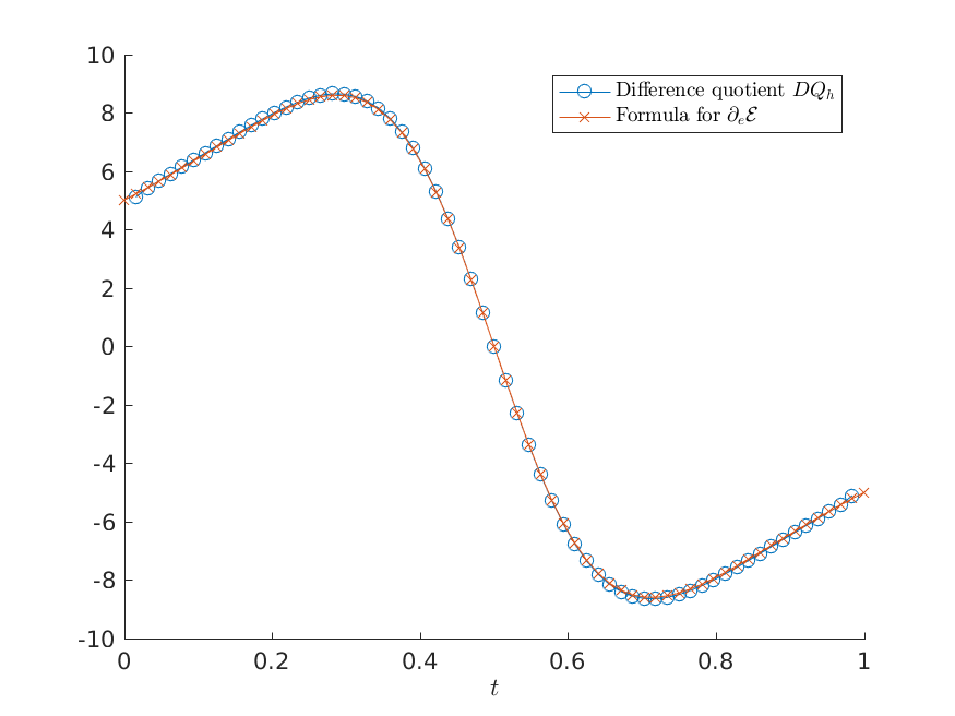
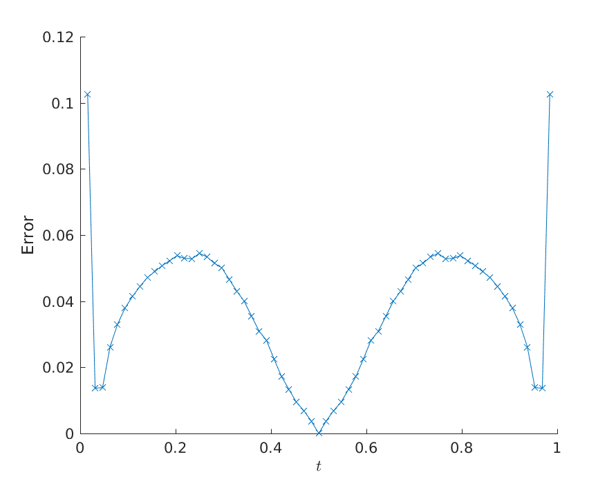
where, $\theta$ is again defined by $\theta(t):=\arcsin\left(\frac{t}{\sqrt{t^{2}+(t-1)^{2}}}\right)$ . With this choice of $\theta$ we have that the points $X_{1},...,X_{5}$ lie on vertices of our chosen grid for each evaluation of $t$ . We calculate $\mathcal{E}_{h}(t)$ and $(\partial_{e}J^{*})_{h}(u_{h}(t))$ for $t\in\left\{\frac{m}{2^{5}}:m\in\mathbb{N}_{0},m\leq 2^{5}\right\}$ . In Figure 3, we plot $\mathcal{E}_{h}(t)$ . The values $(\partial_{e}J^{*})_{h}(u_{h}(t))$ with the difference quotient of $\mathcal{E}_{h}(t)$ and also the difference between them are given in Figure 4. One may calculate that the relative error has a maximum of $2\%$ at the boundary and is below $1\%$ for the interior.

4.1.3 Experiment for simple particles not lying on vertices of the grid

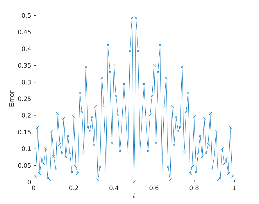
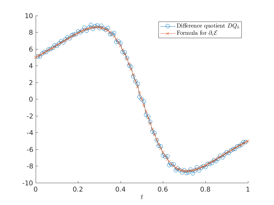
We now provide a perturbation of the above experiment. This experiment is to demonstrate that when the constraint points do not lie on the vertices of the grid, the difference quotient becomes a less reliable method. For this experiment we choose $t\in\{\frac{m}{100}:m\in\mathbb{N}_{0},m\leq 100\}$ . We plot the same quantities as in the previous experiment. In Figure 5, we plot $\mathcal{E}_{h}(t)$ , we notice it has the same characteristic shape as the previous experiment. For Figure 6, we plot $(\partial_{e}J^{*})_{h}(u_{h}(t))$ with the difference quotient of $\mathcal{E}_{h}(t)$ and also the difference between them. We notice that here, the difference quotient does not match the formula as well as in the previous experiment.

4.1.4 Experiment for non-trivial particles

This experiment now deals with two non-trivial particles whereby there is little chance of the points lying on vertices unless one is tailoring the grid to the points. We will see that the difference quotients become highly unreliable. We describe the base of the particle $\mathcal{C}_{1}$ with centre $X_{\mathcal{G}_{1}}=(0,0,1)^{T}$ . We have that $\mathcal{C}_{1}=\{X_{i}\}_{i=1}^{8}$ with

\begin{split}X_{1}=&(0.5,0,\sqrt{1-0.5^{2}})^{T},\\ X_{3}=&(0.25,0.25,\sqrt{1-0.25^{2}-0.25^{2}})^{T},\\ X_{5}=&(0.25,-0.25,\sqrt{1-0.25^{2}-0.25^{2}})^{T},\\ X_{7}=&(0,0.125,\sqrt{1-0.125^{2}})^{T},\end{split}\quad\quad\begin{split}X_{2}=&(-0.5,0,\sqrt{1-0.5^{2}})^{T},\\ X_{4}=&(-0.25,0.25,\sqrt{1-0.25^{2}-0.25^{2}})^{T},\\ X_{6}=&(-0.25,-0.25,\sqrt{1-0.25^{2}-0.25^{2}})^{T},\\ X_{8}=&(0,-0.125,\sqrt{1-0.125^{2}})^{T},\end{split}

and $(Z_{1})_{i}=1-\frac{1}{5}(X_{i})_{1}^{2}$ for $i=1,...,8$ . We let

\mathcal{C}_{2}:=\{x=(x_{1},x_{2},x_{3})^{T}\in\Gamma:(x_{1},x_{3},-x_{2})^{T}\in\mathcal{C}_{1}\},

with $(Z_{2})_{i}=1-\frac{1}{5}(X_{i})_{1}^{2}$ for $i=1,...,8$ .

We consider the rotation of $\mathcal{C}_{1}$ about the north pole, we write $\mathcal{C}_{1}(t):=\mathcal{C}(0,\frac{\pi}{2}t)$ . We calculate the quantities $\mathcal{E}_{h}(t)$ and $(\partial_{e}J^{*})_{h}(u_{h}(t))$ for $t\in\{\frac{m}{2^{4}}:m\in N_{0},m\leq 2^{5}\}$ . We plot $\mathcal{E}(t)$ in Figure 7. In Figure 8 we plot $(\partial_{e}J^{*})_{h}(u_{h}(t))$ and the central difference quotient for $\mathcal{E}_{h}(t)$ .

4.1.5 Experiment to observe the numerical error of a trivial system

We notice that the difference quotient in the previous experiment is extremely noisy, in this experiment, we consider a perturbation of the above experiment, where we remove $\mathcal{C}_{2}$ so that, in light of Corollary 3.15, we are approximating zero. The quantities from this experiment are plotted in Figure 9 where it is seen that there are moderately large perturbations from the average of the energy and the derivative is quite small, as expected.

4.1.6 Application of formula

We now give the results of a numerical experiment which shows that for a perturbation of our non-trivial particles, they demonstrate a preferential orientation. The idea of our experiment is to consider a particle based at a pole and a particle based at the equator. We then calculate the derivative of the energy as the particle at the pole is moved towards the particle at the equator. This experiment is then redone after rotating the particle at the pole by $\frac{\pi}{2}$ . We define the particle $\mathcal{C}_{1}=\{X_{i}\}_{i=1}^{8}$ by

\begin{split}X_{1}=&(0.3,0,\sqrt{1-0.3^{2}})^{T},\\ X_{3}=&(0.15,0.15,\sqrt{1-0.15^{2}-0.15^{2}})^{T},\\ X_{5}=&(0.15,-0.15,\sqrt{1-0.15^{2}-0.15^{2}})^{T},\\ X_{7}=&(0,0.075,\sqrt{1-0.075^{2}})^{T},\end{split}\quad\quad\begin{split}X_{2}=&(-0.3,0,\sqrt{1-0.3^{2}})^{T},\\ X_{4}=&(-0.15,0.15,\sqrt{1-0.15^{2}-0.15^{2}})^{T},\\ X_{6}=&(-0.15,-0.15,\sqrt{1-0.15^{2}-0.15^{2}})^{T},\\ X_{8}=&(0,-0.075,\sqrt{1-0.075^{2}})^{T},\end{split}

and $(Z_{1})_{i}=1-0.9(X_{i})_{1}^{2}$ for $i=1,...,8$ . We give this centre $X_{\mathcal{G}_{1}}:=(0,0,1)^{T}$ . We define $\mathcal{C}_{2}$ by

\mathcal{C}_{2}:=\{x=(x_{1},x_{2},x_{3})^{T}\in\Gamma:(x_{1},x_{3},-x_{2})^{T}\in\mathcal{C}_{1}\},

with $(Z_{2})_{i}=1-10(X_{i})_{1}^{2}$ for $i=1,...,8$ and centre .

We calculate the derivative at $0\in\prod_{i=1}^{2}(\mathbb{R}\times T_{X_{\mathcal{G}_{i}}}\Gamma)$ in direction $e=(0,\tau,0,0)$ , where $\tau=(0,1,0)^{T}\in T_{X_{\mathcal{G}_{1}}}$ represents the translation of $\mathcal{C}_{1}$ in the direction $\tau$ .

We then calculate the derivative at $p:=(\frac{\pi}{2},0,0,0)$ in the same direction $e$ .

We find that

(\partial_{e}J^{*})_{h}(0)\approx-10.6729\quad\mbox{and}\quad(\partial_{e}J^{*})_{h}(p)\approx\mbox{18.5636}.

This shows that the orientation affects whether the particles are attracted to each other, with one orientation being repulsive and the other attractive. In Figure 10 we give the numerical approximations for membranes $u(0)$ and $u(p)$ .

5 Conclusion

In this article we have shown the differentiability of $\mathcal{E}(p)$ , the membrane mediated interaction energy for a near spherical membrane with particles attached at points which depend smoothly on $p$ . Further to showing the differentiability, we have given an explicit formula to calculate the derivative and give numerical examples which demonstrate that this formula would appear to be more robust than a difference quotient approach.

It would be of interest to extend this analysis for particles which are able to move more generally, tilting and moving out from the surface. Furthermore it is desirable to consider the problem for inequality constraints on the ’interior’ of a particle. Finally, one could analyse higher order derivatives of the energy so that one could determine stability of a given configuration.

Acknowledgements

The work of CME was partially supported by the Royal Society via a Wolfson Research Merit Award. The research of PJH was funded by the Engineering and Physical Sciences Research Council grant EP/H023364/1 under the MASDOC centre for doctoral training at the University of Warwick.

Appendix A The pullback to a reference domain

We give some general results on the calculation of the composition of pullbacks and derivatives, where we consider that the image and domain of the diffeomorphism need not be the same. As we are working with different surfaces, we will need to make clear to which surface geometric quantities belong to, this is done with a superscript of the surface, e.g. $H^{\Gamma_{1}}$ is the mean curvature of $\Gamma_{1}$ and $H^{{\Gamma_{0}}}$ the mean curvature of ${\Gamma_{0}}$ . Consider the case of $\Gamma_{0}$ and $\Gamma_{1}$ being $C^{k}$ , compact surfaces, with $\mathrm{X}\colon\Gamma_{0}\to\Gamma_{1}$ a $C^{k}$ -diffeomorphism, where we require $k\geq 2$ .

Given some function $u\colon\Gamma_{1}\to\mathbb{R}$ we wish to obtain expressions for $(\nabla_{\Gamma_{1}}u)\circ\mathrm{X}$ and $(\underline{D}^{2}_{\Gamma_{1}}u)\circ\mathrm{X}$ . The first part of this is developed in [7], where also the trace of the second quantity, the Laplace-Beltrami, is calculated. Although for the model we consider in this work, the surface Hessian is not required, we compute it for completion as it may arise in other elastic type models, where the Hessian regularly arises. We choose to do this in an method which avoids integration by parts so that surfaces with boundary may be considered.

Lemma A.1.

Let $u\in H^{1}(\Gamma_{1})$ , then $u\circ\mathrm{X}\in H^{1}(\Gamma_{0})$ and

(\nabla_{\Gamma_{1}}u)\circ\mathrm{X}=\left(\nabla_{\Gamma_{0}}\mathrm{X}+\nu^{\Gamma_{1}}\circ\mathrm{X}\otimes\nu^{\Gamma_{0}}\right)^{-T}\nabla_{\Gamma_{0}}(u\circ\mathrm{X})=\nabla_{\Gamma_{0}}\mathrm{X}G_{\Gamma_{0}}^{-1}\nabla_{\Gamma_{0}}(u\circ\mathrm{X}),

where $G_{\Gamma_{0}}:=\nabla_{\Gamma_{0}}\mathrm{X}^{T}\nabla_{\Gamma_{0}}\mathrm{X}+\nu^{\Gamma_{0}}\otimes\nu^{\Gamma_{0}}$ .

The proof is shown in Lemma 3.2 of [7]. We write $B:=\nabla_{\Gamma_{0}}\mathrm{X}+\nu^{\Gamma_{1}}\circ\mathrm{X}\otimes\nu^{\Gamma_{0}}$ , which satisfies

B^{T}B=G_{\Gamma_{0}}.

This gives a simpler form of the above lemma,

(\nabla_{\Gamma_{1}}u)\circ\mathrm{X}=B^{-T}\nabla_{{\Gamma_{0}}}(u\circ\mathrm{X}).

Lemma A.2.

Let $u\in H^{2}(\Gamma_{1})$ , then $u\circ\mathrm{X}\in H^{2}(\Gamma_{0})$ and for $i,j=1,...,n+1$

	$\displaystyle(\underline{D}_{i}^{\Gamma_{1}}\underline{D}_{j}^{\Gamma_{1}}u)\circ\mathrm{X}=$	$\displaystyle\frac{1}{b}{\rm div}_{\Gamma_{0}}\left(bB^{-1}(B^{-T}\nabla_{\Gamma_{0}}\hat{u})_{j}\right)_{i}$
		$\displaystyle+(H^{\Gamma_{1}}\circ\mathrm{X}-H^{\Gamma_{0}})(\nu_{i}^{\Gamma_{1}}\circ\mathrm{X})(B^{-T}\nabla_{\Gamma_{0}}\hat{u})_{j},$

where $b=\det(B),\,b_{ij}=B_{ij}$ and $b^{ij}=\left(B^{-1}\right)_{ij}$ .

Proof.

We write $\hat{u}:=u\circ\mathrm{X}$ and where indices are repeated in a product, summation is assumed. We now make use of the preceding lemma to obtain,

\displaystyle\underline{D}_{i}^{\Gamma_{1}}\underline{D}^{\Gamma_{1}}_{j}u\circ\mathrm{X}=

\displaystyle b^{li}\underline{D}_{l}^{\Gamma_{0}}\left(b^{kj}\underline{D}_{k}^{\Gamma_{0}}\hat{u}\right).

We now put this into something similar to a divergence form,

\displaystyle\underline{D}_{i}^{\Gamma_{1}}\underline{D}_{j}^{\Gamma_{1}}u\circ\mathrm{X}=

\displaystyle\frac{1}{b}\underline{D}_{l}^{\Gamma_{0}}\left(bb^{li}b^{kj}\underline{D}_{k}^{\Gamma_{0}}\hat{u}\right)-\frac{1}{b}\underline{D}_{l}^{\Gamma_{0}}\left(b\right)b^{li}b^{kj}\underline{D}_{k}^{\Gamma_{0}}\hat{u}-\underline{D}_{l}^{\Gamma_{0}}\left(b^{li}\right)b^{kj}\underline{D}_{k}^{\Gamma_{0}}\hat{u}.

In [7], it is calculated

\underline{D}_{l}^{\Gamma_{0}}b^{li}=-b^{lm}\underline{D}_{l}^{\Gamma_{0}}b_{mf}b^{fi},~~\frac{1}{b}\underline{D}_{l}^{\Gamma_{0}}b=b^{fm}\underline{D}_{l}^{\Gamma_{0}}b_{mf},

inserting these into the above gives,

\underline{D}_{i}^{\Gamma_{1}}\underline{D}_{j}^{\Gamma_{1}}u\circ\mathrm{X}=\frac{1}{b}\underline{D}_{l}^{\Gamma_{0}}\left(bb^{li}b^{kj}\underline{D}_{k}^{\Gamma_{0}}\hat{u}\right)-b^{fm}\underline{D}_{l}^{\Gamma_{0}}b_{mf}b^{li}b^{kj}\underline{D}_{k}^{\Gamma_{0}}\hat{u}+b^{lm}\underline{D}_{l}^{\Gamma_{0}}b_{mf}b^{fi}b^{kj}\underline{D}_{k}^{\Gamma_{0}}\hat{u}.

Since we are summing over $f,\,k,\,l$ and $m$ in the above, it is possible to swap the indices, in particular we swap $f$ and $l$ in the second term. We now consider the terms

\begin{split}b^{lm}\underline{D}_{l}^{\Gamma_{0}}b_{mf}b^{fi}b^{kj}\underline{D}_{k}^{\Gamma_{0}}\hat{u}-&b^{lm}\underline{D}_{f}^{\Gamma_{0}}b_{ml}b^{fi}b^{kj}\underline{D}_{k}^{\Gamma_{0}}\hat{u}\\ &=b^{lm}b^{fi}\left(b^{kj}\underline{D}_{k}^{\Gamma_{0}}\hat{u}\right)\left(\underline{D}_{l}^{\Gamma_{0}}b_{mf}-\underline{D}_{f}^{\Gamma_{0}}b_{ml}\right).\end{split}

(A.1)

In order to simplify this, we will use the definition of $B$ and swap the order of derivatives. As in [7], one calculates

	$\displaystyle\underline{D}_{l}^{\Gamma_{0}}b_{mf}-\underline{D}_{f}^{\Gamma_{0}}b_{ml}=$	$\displaystyle\left(\underline{D}_{l}^{\Gamma_{0}}(\nu_{m}^{\Gamma_{1}}\circ\mathrm{X})-\left(\mathcal{H}^{\Gamma_{0}}\nabla_{\Gamma_{0}}\mathrm{X}_{m}\right)_{l}\right)\nu_{f}^{\Gamma_{0}}$
		$\displaystyle+\left(\left(\mathcal{H}^{\Gamma_{0}}\nabla_{\Gamma_{0}}\mathrm{X}_{m}\right)_{f}-\underline{D}_{f}^{\Gamma_{0}}(\nu_{m}^{\Gamma_{1}}\circ\mathrm{X})\right)\nu_{l}^{\Gamma_{0}}.$

We now use this to simplify (A.1). We will make use of the relation $b^{ki}\nu_{k}^{\Gamma_{0}}=\nu_{i}^{\Gamma_{1}}\circ\mathrm{X}$ . We calculate each part,

	$\displaystyle b^{lm}b^{fi}\underline{D}_{l}^{\Gamma_{0}}(\nu_{m}^{\Gamma_{1}}\circ\mathrm{X})\nu_{f}^{\Gamma_{0}}=$	$\displaystyle(\nu_{i}^{\Gamma_{1}}\circ\mathrm{X})(B^{-T}(\nabla_{\Gamma_{1}}\nu_{m})\circ\mathrm{X})_{m}$
	$\displaystyle=$	$\displaystyle(H^{\Gamma_{1}}\nu_{i}^{\Gamma_{1}})\circ\mathrm{X},$

	$\displaystyle b^{lm}b^{fi}(\mathcal{H}^{\Gamma_{0}}\nabla_{\Gamma_{0}}\mathrm{X}_{m})_{l}\nu_{f}^{\Gamma_{0}}=$	$\displaystyle b^{lm}b^{fi}\mathcal{H}^{\Gamma_{0}}_{lk}\underline{D}_{k}^{\Gamma_{0}}\mathrm{X}_{m}\nu_{f}^{\Gamma_{0}}$
	$\displaystyle=$	$\displaystyle b^{lm}b^{fi}\mathcal{H}^{\Gamma_{0}}_{lk}b_{mk}\nu_{f}^{\Gamma_{0}}$
	$\displaystyle=$	$\displaystyle H^{\Gamma_{0}}(\nu^{\Gamma_{1}}_{i}\circ\mathrm{X}),$

	$\displaystyle b^{lm}b^{fi}(\mathcal{H}^{\Gamma_{0}}\nabla_{\Gamma_{0}}\mathrm{X}_{m})_{f}\nu_{l}^{\Gamma_{0}}=$	$\displaystyle b^{lm}b^{fi}\mathcal{H}^{\Gamma_{0}}_{fk}\underline{D}_{k}^{\Gamma_{0}}\mathrm{X}_{m}\nu_{l}^{\Gamma_{0}}$
	$\displaystyle=$	$\displaystyle b^{lm}b^{fi}\mathcal{H}^{\Gamma_{0}}_{fk}b_{mk}\nu_{l}^{\Gamma_{0}}$
	$\displaystyle=$	$\displaystyle b^{fi}\mathcal{H}^{\Gamma_{0}}_{fl}\nu_{l}^{\Gamma_{0}}=0,$

	$\displaystyle b^{lm}b^{fi}(\nu^{\Gamma_{1}}_{m}\circ\mathrm{X})\nu_{l}^{\Gamma_{1}}=$	$\displaystyle(\nu_{m}^{\Gamma_{1}}\circ\mathrm{X})(B^{-T}\nabla_{\Gamma_{0}}(\nu^{\Gamma_{1}}\circ\mathrm{X}))_{i}$
	$\displaystyle=$	$\displaystyle(\nu_{m}^{\Gamma_{1}}\circ\mathrm{X})\mathcal{H}^{\Gamma_{1}}_{mi}\circ\mathrm{X}=0.$

This then gives

b^{lm}b^{fi}\left(b^{kj}\underline{D}_{k}^{\Gamma_{0}}\hat{u}\right)\left(\underline{D}_{l}^{\Gamma_{0}}b_{mf}-\underline{D}_{f}^{\Gamma_{0}}b_{ml}\right)=((H^{\Gamma_{1}}\circ\mathrm{X})-H^{\Gamma_{0}})(\nu_{i}^{\Gamma_{1}}\circ\mathrm{X})(B^{-T}\nabla_{\Gamma_{0}}\hat{u})_{j},

which completes the result. ∎

Remark A.3.

By taking the trace of $\underline{D}_{\Gamma_{1}}^{2}u\circ\mathrm{X}$ , one obtains

(\Delta_{\Gamma_{1}}u)\circ\mathrm{X}=\frac{1}{b}{\rm div}_{\Gamma_{0}}(bG_{\Gamma_{0}}^{-1}\nabla_{\Gamma_{0}}(u\circ\mathrm{X})).

Appendix B Implicit function theorem

We give the version of the implicit function theorem we use in Theorem 3.9. The result is taken from [8, Theorem 7.13-1].

Theorem B.1.

Let $\mathcal{X}$ be a normed vector space, $\mathcal{Y}$ and $\mathcal{Z}$ Banach spaces with $\Omega\subset\mathcal{X}\times\mathcal{Y}$ open with $(a,b)\in\Omega$ . Let $f\in C(\Omega;\mathcal{Z})$ with $f(a,b)=0$ , $\frac{\partial f}{\partial y}(x,y)\in\mathcal{L}(\mathcal{Y};\mathcal{Z})$ exists at all points $(x,y)\in\Omega$ and $\frac{\partial f}{\partial y}\in C(\Omega;\mathcal{L}(\mathcal{Y};\mathcal{Z})),$ $\frac{\partial f}{\partial y}(a,b)$ is a bijection, so that $\left(\frac{\partial f}{\partial y}(a,b)\right)^{-1}\in\mathcal{L}(\mathcal{Z};\mathcal{Y})$ .

1.

Then there is an open neighbourhood $V$ of $a$ in $\mathcal{X}$ , a neighbourhood $W$ of $b$ in $\mathcal{Y}$ and $g\in C(V;W)$ such that $V\times W\subset\Omega$ and $\{(x,y)\in V\times W:f(x,y)=0\}=\{(x,y)\in V\times W:y=g(x)\}$ .

Assume in addition that $f$ is differentiable at $(a,b)\in\Omega$ . Then $g$ is differentiable at $a$ and

g^{\prime}(a)=-\left(\frac{\partial f}{\partial y}(a,b)\right)^{-1}\frac{\partial f}{\partial x}(a,b)\in\mathcal{L}(\mathcal{X};\mathcal{Y}).

3.

Assume in addition that $f\in C^{k}(\Omega;\mathcal{Z})$ for some $k\geq 1$ . Then there is an open neighbourhood $\tilde{V}\subset V$ of $a$ in $\mathcal{X}$ and neighbourhood $\tilde{W}\subset W$ of $b$ in $\mathcal{Y}$ such that $\frac{\partial f}{\partial y}(x,y)\in\mathcal{L}(\mathcal{Y};\mathcal{Z})$ is a bijection, so that $\left(\frac{\partial f}{\partial y}(x,y)\right)^{-1}\in\mathcal{L}(\mathcal{Z};\mathcal{Y})$ at each $(x,y)\in\tilde{V}\times\tilde{W}$ , $g\in C^{k}(\tilde{V};\mathcal{Y})$ , $g^{\prime}(x)=-\left(\frac{\partial f}{\partial y}(x,g(x))\right)^{-1}\frac{\partial f}{\partial x}(x,g(x))\in\mathcal{L}(\mathcal{X};\mathcal{Y})$ for each $x\in\tilde{V}$ .

Appendix C Elliptic regularity

We first show, for arbitrary surfaces, that $\Delta_{\Gamma}u\in W^{1,p}(\Gamma)$ for $p\leq 2$ gives $u\in W^{3,p}(\Gamma)$ .

Proposition C.1.

Suppose $u\in H^{1}(\Gamma)$ with $\Delta_{\Gamma}u\in W^{1,p}(\Gamma)$ for some $p\in(1,2]$ and $\Gamma$ is $C^{3}$ , then there is a $C>0$ independent of $u$ such that for each $i,j=1,2,3$ ,

\|\underline{D}_{i}\underline{D}_{j}u\|_{1,p}\leq C\left(\|\underline{D}_{j}\Delta_{\Gamma}u\|_{0,p}+\|\Delta_{\Gamma}u\|_{0,2}+\|\nabla_{\Gamma}u\|_{0,2}\right).

Proof.

We make use of the following inf-sup condition, shown in [13]:

\exists\gamma>0:\gamma\|\xi\|_{1,p}\leq\sup_{\eta\in W^{1,q}(\Gamma)}\frac{\int_{\Gamma}\nabla_{\Gamma}\eta\cdot\nabla_{\Gamma}\xi+\eta\xi}{\|\eta\|_{1,q}}\quad\forall\xi\in W^{1,p}(\Gamma).

By the fact that $\Gamma$ has finite measure, it holds that $\|\underline{D}_{i}\underline{D}_{j}u\|_{0,p}\leq C\|\underline{D}_{i}\underline{D}_{j}u\|_{0,2}$ which we know is controlled by $\|\Delta_{\Gamma}u\|_{0,2}+\sqrt{\|\mathcal{H}H-2\mathcal{H}^{2}\|_{0,\infty}}\|\nabla_{\Gamma}u\|_{0,2}$ , [11]. It is then sufficient to show that $\int_{\Gamma}\nabla_{\Gamma}\underline{D}_{i}\underline{D}_{j}u\cdot\nabla_{\Gamma}\eta$ is bounded appropriately. One may calculate

	$\displaystyle\int_{\Gamma}\nabla_{\Gamma}\underline{D}_{i}\underline{D}_{j}u\cdot\nabla_{\Gamma}\eta=\int_{\Gamma}$	$\displaystyle\underline{D}_{j}\Delta_{\Gamma}u\underline{D}_{i}\eta$
		$\displaystyle+\left(\left(\mathcal{H}\nabla_{\Gamma}\underline{D}_{k}u\right)_{j}\nu_{k}-\left(\mathcal{H}\nabla_{\Gamma}\underline{D}_{k}u\right)_{k}\nu_{i}-\underline{D}_{k}\left[\left(\mathcal{H}\nabla_{\Gamma}u\right)_{k}\nu_{j}\right]\right)\underline{D}_{i}\eta$
		$\displaystyle-\underline{D}_{k}\underline{D}_{j}u\left(\mathcal{H}\nabla_{\Gamma}\eta\right)_{k}\nu_{i}-\left(\mathcal{H}\nabla_{\Gamma}\underline{D}_{j}u\right)_{k}\nu_{i}\underline{D}_{k}\eta.$

This follows from repeatedly applying integration by parts and swapping the order of derivatives. Applying Hölder’s inequality, the result immediately follows. ∎

Proposition C.2.

Let $u\in H^{2}(\Gamma)$ be the unique solution of Problem 2.3, then it holds that for any $p<2$ , $u\in W^{3,p}(\Gamma)$ .

Proof.

By [18, Theorem 2.34] and the arguments presented in [17, Section 5], it is clear that there is $\bar{p}\in\mathbb{R}$ and $\lambda\in\mathbb{R}^{K}$ such that

a(u,v)+\bar{p}\int_{\Gamma}v+\lambda\cdot v|_{\mathcal{C}}=0~~\forall v\in H^{2}(\Gamma).

Let $\eta:=-\Delta_{\Gamma}u-\frac{2}{R^{2}}u\in L^{2}(\Gamma)$ , then for any $v\in H^{2}(\Gamma)$ ,

a(u,v)=\int_{\Gamma}(-\kappa\Delta_{\Gamma}v+\sigma v)\eta=-\lambda\cdot v|_{\mathcal{C}}-\bar{p}\int_{\Gamma}v.

Let $\phi\in C^{\infty}(\Gamma)$ and consider the inverse Laplace type map $G\colon L^{2}(\Gamma)\to H^{2}(\Gamma)$ such that $G\colon\phi\mapsto v$ where $-\kappa\Delta_{\Gamma}v+\sigma v=\phi$ . Via a local argument, it may be seen that for any $q>2$ , $\|v\|_{0,\infty}\leq C\|\phi\|_{-1,q}$ [33]. Hence

	$\displaystyle\langle\phi,\eta\rangle$	$\displaystyle=\int_{\Gamma}\phi\eta=\int_{\Gamma}(-\kappa\Delta_{\Gamma}v+\sigma v)\eta$
		$\displaystyle=-\lambda\cdot v\|_{\mathcal{C}}-\bar{p}\int_{\Gamma}v$
		$\displaystyle\leq\\|\lambda\\|_{\mathbb{R}^{M}}\\|v\\|_{0,\infty}+\|\bar{p}\|\\|v\\|_{0,1}$
		$\displaystyle\leq C\\|\phi\\|_{-1,q}.$

Thus we have shown that $\eta$ represents a bounded linear operator on $W^{-1,q}(\Gamma)$ , thus we have shown that $-\Delta_{\Gamma}u-\frac{2}{R^{2}}u\in W^{1,q^{*}}(\Gamma)$ . In particular, by Proposition C.1, it holds that $u\in W^{3,q^{*}}(\Gamma)$ . Since $q^{*}<2$ is arbitrary, the result is complete. ∎

References

[1] R. A. Adams and J. J. Fournier, Sobolev spaces, Elsevier, 2003.
[2] M. Alkämper, A. Dedner, R. Klöfkorn, and M. Nolte, The DUNE-ALUGrid Module., Archive of Numerical Software, 4 (2016), pp. 1–28.
[3] A.-F. Bitbol, D. Constantin, and J.-B. Fournier, Membrane-mediated interactions, Physics of Biological Membranes, (2018), pp. 311–350.
[4] M. Blatt, A. Burchardt, A. Dedner, C. Engwer, J. Fahlke, B. Flemisch, C. Gersbacher, C. Gräser, F. Gruber, C. Grüninger, et al., The distributed and unified numerics environment, version 2.4, Archive of Numerical Software, 4 (2016), pp. 13–29.
[5] G. Buttazzo and S. A. Nazarov, An optimization problem for the biharmonic equation with Sobolev conditions, Journal of Mathematical Sciences, 176 (2011), p. 786.
[6] P. B. Canham, The minimum energy of bending as a possible explanation of the biconcave shape of the human red blood cell, Journal of Theoretical Biology, 26 (1970), pp. 61–81.
[7] L. Church, A. Djurdjevac, and C. M. Elliott, A domain mapping approach for elliptic equations posed on random bulk and surface domains, Numerische Mathematik, https://doi.org/10.1007/s00211-020-01139-7 (2020).
[8] P. G. Ciarlet, Linear and Nonlinear Functional Analysis with Applications, Society for Industrial and Applied Mathematics, Philadelphia, PA, USA, 2013.
[9] S. Dharmavaram and L. E. Perotti, A Lagrangian formulation for interacting particles on a deformable medium, Computer Methods in Applied Mechanics and Engineering, 364 (2020), p. 112949.
[10] P. G. Dommersnes and J.-B. Fournier, The many-body problem for anisotropic membrane inclusions and the self-assembly of “saddle” defects into an “egg carton”, Biophysical Journal, 83 (2002), pp. 2898 – 2905.
[11] G. Dziuk and C. M. Elliott, Finite element methods for surface PDEs, Acta Numer., 22 (2013), pp. 289–396.
[12] C. M. Elliott, H. Fritz, and G. Hobbs, Small deformations of Helfrich energy minimising surfaces with applications to biomembranes, Math. Models Methods Appl. Sci., 27 (2017), pp. 1547–1586.
[13] C. M. Elliott, H. Fritz, and G. Hobbs, Second order splitting for a class of fourth order equations, Mathematics of Computation, 88 (2019), pp. 2605–2634.
[14] C. M. Elliott, C. Gräser, G. Hobbs, R. Kornhuber, and M.-W. Wolf, A variational approach to particles in lipid membranes, Archive for Rational Mechanics and Analysis, 222 (2016), pp. 1011–1075.
[15] C. M. Elliott and L. Hatcher, Domain formation via phase separation for spherical biomembranes with small deformations, arXiv preprint arXiv:1912.10317, (2019).
[16] C. M. Elliott, L. Hatcher, and P. J. Herbert, Small deformations of spherical biomembranes, in The Role of Metrics in the Theory of Partial Differential Equations, vol. 85 of Advanced Studies in Pure Mathematics, Tokyo, Japan, 2020, Mathematical Society of Japan, pp. 39–61.
[17] C. M. Elliott and P. J. Herbert, Second order splitting of a class of fourth order PDEs with point constraints, Math. Comp., (2020).
[18] A. Ern and J. L. Guermond, Theory and Practice of Finite Elements, Applied Mathematical Sciences, Springer New York, 2004.
[19] J.-B. Fournier and P. Galatola, High-order power series expansion of the elastic interaction between conical membrane inclusions, The European Physical Journal E, 38 (2015), p. 86.
[20] M. Goulian, R. Bruinsma, and P. Pincus, Long-range forces in heterogeneous fluid membranes, Europhysics Letters (EPL), 22 (1993), pp. 145–150.
[21] N. Gov, Guided by curvature: Shaping cells by coupling curved membrane proteins and cytoskeletal forces, Philosophical Transactions of the Royal Society B: Biological Sciences, 373 (2018).
[22] C. Gräser and T. Kies, On differentiability of the membrane-mediated mechanical interaction energy of discrete-continuum membrane-particle models, arXiv preprint arXiv:1711.1119, (2017).
[23] C. Gräser and T. Kies, Discretization error estimates for penalty formulations of a linearized Canham–Helfrich-type energy, IMA Journal of Numerical Analysis, 39 (2019), pp. 626–649.
[24] P. Hartman, Ordinary differential equations, vol. 38 of Classics in Applied Mathematics, Society for Industrial and Applied Mathematics (SIAM), Philadelphia, PA, 2002.
[25] W. Helfrich, Elastic properties of lipid bilayers: theory and possible experiments, Zeitschrift für Naturforschung C, 28 (1973), pp. 693–703.
[26] W. M. Henne, E. Boucrot, M. Meinecke, E. Evergren, Y. Vallis, R. Mittal, and H. T. McMahon, FCHo proteins are nucleators of clathrin-mediated endocytosis, Science, 328 (2010), pp. 1281–1284.
[27] W. M. Henne, H. M. Kent, M. G. Ford, B. G. Hegde, O. Daumke, P. J. G. Butler, R. Mittal, R. Langen, P. R. Evans, and H. T. McMahon, Structure and analysis of FCHo2 F-BAR domain: A dimerizing and membrane recruitment module that effects membrane curvature, Structure, 15 (2007), pp. 839 – 852.
[28] T. Kies, Gradient methods for membrane-mediated particle interactions, PhD thesis, Institut für Mathematik, Freie Universität Berlin, 2019.
[29] K. Kim, J. Neu, and G. Oster, Curvature-mediated interactions between membrane proteins, Biophysical Journal, 75 (1998), pp. 2274 – 2291.
[30] K. S. Kim, J. Neu, and G. Oster, Effect of protein shape on multibody interactions between membrane inclusions, Phys. Rev. E, 61 (2000), pp. 4281–4285.
[31] K. Larsson and M. G. Larson, A continuous/discontinuous Galerkin method and a priori error estimates for the biharmonic problem on surfaces, Mathematics of Computation, 86 (2017), pp. 2613–2649.
[32] R. Mathias, S. Gabriel, and L. Tony, Free Energy Computations: A Mathematical Perspective, World Scientific, 2010.
[33] J. Necas, Direct methods in the theory of elliptic equations, Springer Science & Business Media, 2011.
[34] A. Reusken, Stream function formulation of surface stokes equations, IMA Journal of Numerical Analysis, 40 (2020), pp. 109–139.
[35] Y. Schweitzer and M. M. Kozlov, Membrane-mediated interaction between strongly anisotropic protein scaffolds, PLOS Computational Biology, 11 (2015), pp. 1–17.
[36] T. R. Weikl, Membrane-mediated cooperativity of proteins, Annual review of physical chemistry, 69 (2018), pp. 521–539.
[37] T. R. Weikl, M. M. Kozlov, and W. Helfrich, Interaction of conical membrane inclusions: Effect of lateral tension, Phys. Rev. E, 57 (1998), pp. 6988–6995.
[38] T. J. Willmore, Note on embedded surfaces, An. Sti. Univ.“Al. I. Cuza” Iasi Sect. I a Mat.(NS) B, 11 (1965), pp. 493–496.
[39] C. Yolcu, R. C. Haussman, and M. Deserno, The effective field theory approach towards membrane-mediated interactions between particles, Advances in Colloid and Interface Science, 208 (2014), pp. 89 – 109.

	$\displaystyle\partial_{e}\mathcal{V}(t,0,y)=$	$\displaystyle\partial_{s}\mathcal{V}(t,se,y)\|_{s=0}$
	$\displaystyle=$	$\displaystyle\partial_{s}\left(\mathcal{V}(t,se,\phi_{i}(p+se,\cdot)\circ\phi_{i}(p,\cdot)^{-1}(y))\right)\|_{s=0}$
		$\displaystyle+\partial_{s}\left(\mathcal{V}(t,se,x)-\mathcal{V}(t,se,\phi_{i}(p+se,\cdot)\circ\phi_{i}(p,\cdot)^{-1}(y))\right)\|_{s=0}$
	$\displaystyle=$	$\displaystyle\partial_{s}\left(\mathcal{V}(t,se,\phi_{i}(p+se,\cdot)\circ\phi_{i}(p,\cdot)^{-1}(y))\right)\|_{s=0}$
		$\displaystyle+\partial_{s}\left(\mathcal{V}(t,se,y)-\mathcal{V}(t,se,\phi_{i}(p+se,\cdot)\circ\phi_{i}(p,\cdot)^{-1}(y))\right)\|_{s=0}.$

	$\displaystyle\|\partial_{e}J^{*}(0,\tilde{u})-\partial_{e}\mathcal{E}(p)\|\leq C\\|\nabla_{\Gamma}V\\|_{0,\infty}\Big($	$\displaystyle\\|\Delta_{\Gamma}(u-\tilde{u})\\|_{1,p}\\|\nabla_{\Gamma}u\\|_{1,q}$
		$\displaystyle+\\|\Delta_{\Gamma}(u-\tilde{u})\\|_{0,2}\left(\\|\Delta_{\Gamma}\tilde{u}\\|_{0,2}+\\|\Delta_{\Gamma}u\\|_{0,2}\right)$
		$\displaystyle+\\|\nabla_{\Gamma}(u-\tilde{u})\\|_{0,\frac{2-\epsilon}{1-\epsilon}}\\|\Delta_{\Gamma}\tilde{u}\\|_{1,2-\epsilon}$
		$\displaystyle+\\|\nabla_{\Gamma}(u-\tilde{u})\\|_{1,2}\left(\\|\nabla_{\Gamma}u\\|_{1,2}+\\|\nabla_{\Gamma}\tilde{u})\\|_{1,2}\right)\Big).$

	$\displaystyle\langle\phi,\eta\rangle$	$\displaystyle=\int_{\Gamma}\phi\eta=\int_{\Gamma}(-\kappa\Delta_{\Gamma}v+\sigma v)\eta$
		$\displaystyle=-\lambda\cdot v\|_{\mathcal{C}}-\bar{p}\int_{\Gamma}v$
		$\displaystyle\leq\\|\lambda\\|_{\mathbb{R}^{M}}\\|v\\|_{0,\infty}+\|\bar{p}\|\\|v\\|_{0,1}$
		$\displaystyle\leq C\\|\phi\\|_{-1,q}.$

A formula for membrane mediated point particle interactions on near spherical biomembranes

Abstract

1 Introduction

1.1 Outline

1.2 Surface PDE preliminaries

2 Membrane and particle model

2.1 Membrane model

Definition 2.1.

Remark 2.2.

2.2 An energy minimising membrane subject to point constraints

Problem 2.3.

Theorem 2.4.

Remark 2.5.

2.3 A single particle model

Definition 2.6.

2.4 Parametrisation of a single particle

Definition 2.7.

Remark 2.8.

2.5 Configuration of particles

Definition 2.9.

Definition 2.10.

Remark 2.11.

Definition 2.12.

Assumption 2.13.

Definition 2.14 (Membrane configurational energy).

Remark 2.15.

3 Gradient of the energy with respect to configuration changes

Definition 3.1 (Derivative of the configurational energy).

Assumption 3.2.

Definition 3.3.

Remark 3.4.

3.1 The transformed functional and its derivative

Definition 3.5.

Definition 3.6.

Lemma 3.7.

Lemma 3.8.

Proof.

Theorem 3.9.

Proof.

Remark 3.10.

3.2 An explicit formula for the derivative

Definition 3.11.

Proposition 3.12.

Proof.

Corollary 3.13.

Proof.

Theorem 3.14.

Proof.

Corollary 3.15.

Proof.

3.3 Transformations satisfying Assumption 3.2

3.3.1 Rotation of a single particle

3.3.2 A general χ\chi

Definition 3.16 (Equation (2.6) [34]).

Definition 3.17.

Example 3.18.

Lemma 3.19.

Proof.

Definition 3.20.

Proposition 3.21.

Proof.

Proposition 3.22.

Proof.

4 Numerical experiments

Proposition 4.1.

Proof.

4.1 Experiments

Definition 4.2.

4.1.1 Convergence experiment

4.1.2 Experiment for simple particles lying on vertices

4.1.3 Experiment for simple particles not lying on vertices of the grid

4.1.4 Experiment for non-trivial particles

4.1.5 Experiment to observe the numerical error of a trivial system

4.1.6 Application of formula

5 Conclusion

Acknowledgements

Appendix A The pullback to a reference domain

Lemma A.1.

Lemma A.2.

Proof.

3.3.2 A general $\chi$