Single-Trajectory Characterization of Active Swimmers in a Flow.

In Ref. Junot et al. 2019, it was shown that rotational diffusion considerably affects the trajectories of mutant E. coli in a flow. This fact represents a strong motivation to consider the effects of rotational noise in the dynamics of the orientation vector of smooth swimmers. We focus on the model studied in Ref. Junot et al. 2019 in presence of noise, which we refer to as the stochastic active Betherton-Jefferey (SABJ) model from now on. The model describes the behavior of an ellipsoid swimming at a constant speed in a flow. Its dynamics read:

Above, $v_{0}$ is the self-propulsion velocity of the particle, $\mathbf{v}^{F}$ is the local flow velocity, the symbol $\mathbb{1}$ denotes the identity matrix, and $\otimes$ is used to denote tensor products. The number $\beta=(r^{2}-1)/(r^{2}+1)$ is the Betherton parameter, which represents a measure of the geometrical asymmetry of the swimmer ($r$ is the aspect-ratio of the ellipsoidal particle). The components of the tensors $\mathbb{E}$ and $\mathbb{\Omega}$ are given as follows, $E_{ij}(\mathbf{r})=(\partial_{x_{i}}v^{F}_{j}+\partial_{x_{j}}v^{F}_{i})/2$ and $\Omega_{ij}(\mathbf{r})=(\partial_{x_{i}}v^{F}_{j}-\partial_{x_{j}}v^{F}_{i})/2$.

In Eq. (II.1), rotational diffusion is encoded in the diffusion coefficient $D_{R}$ and the Gaussian white noise $\boldsymbol{\xi}_{R}$ which has zero mean and variance $\langle\boldsymbol{\xi}_{R}(t)\otimes\boldsymbol{\xi}_{R}(t^{\prime})\rangle=\mathbb{1}\delta(t-t^{\prime})$. In this work, Eq. (II.1) is interpreted in the Ito sense. The Ito term $-2D_{R}\mathbf{p}$ is thus needed to guarantee the conservation of the norm of $\mathbf{p}$. Note that, although one could also introduce a translational diffusion term in Eq. (1), such contribution can be assumed negligible in typical experimental situations. Consider, for instance, an E. coli bacterium which is few microns length, swimming at a typical speed of $25\text{\,}\mathrm{\SIUnitSymbolMicro m}\text{\,}{\mathrm{s}}^{-1}$. The distance over which it diffuses in $1\text{\,}\mathrm{s}$ is $\approx$0.1\text{\,}\mathrm{\SIUnitSymbolMicro m}$$ to be compared to the $25\text{\,}\mathrm{\SIUnitSymbolMicro m}$ travelled due to its activity.

In Fig. 1 we illustrate our model system, making explicit the way in which geometrical parameters are defined. It is important to remark that the bacterium is a complex object and that the optical determination of $\beta$ is non-trivial. In other words, $\beta$ is an effective parameter and its determination based on imagery alone may not be reliable. However, for an elongated bacterium such as E. coli its expected value should be close to one (see the sketch in Fig. 1(b)). In the same figure, we also show how the Péclet number is defined in presence of shear and Poiseulle flows. The Péclet number plays an important role in numerics because it is the natural dimensionless form of the inverse of the rotational diffusion coefficient, see Sec. IV for more details.

An important role is played by the Markov kernel of the process (1)-(II.1), which we denote by $K(\mathbf{r},\mathbf{p},t|\mathbf{r}^{\prime},\mathbf{p}^{\prime},t^{\prime})$. We focus here on stationary flow profiles in which case the propagtor only depends on $\Delta t=t-t^{\prime}$ due to time-translation invariance. We thus simplify the notations by writing $K(\mathbf{r},\mathbf{p},t|\mathbf{r}^{\prime},\mathbf{p}^{\prime},t^{\prime})=K(\mathbf{r},\mathbf{p},\Delta t|\mathbf{r}^{\prime},\mathbf{p}^{\prime},0)\equiv K(\mathbf{r},\mathbf{p},\Delta t|\mathbf{r}^{\prime},\mathbf{p}^{\prime})$. The propagator satisfies the Fokker-Planck equation $\partial_{t}K=\hat{L}_{FP}K$ with initial condition $K(\mathbf{r},\mathbf{p},0|\mathbf{r}^{\prime},\mathbf{p}^{\prime})=\delta(\mathbf{r}-\mathbf{r}^{\prime})\delta(\mathbf{p}-\mathbf{p}^{\prime})$. The Fokker-Planck operator associated to these dynamics reads

To write (II.1), we condensed the translational part of the motion into $\mathbf{v}(\mathbf{r},\mathbf{p})=v_{0}\mathbf{p}+\mathbf{v}^{F}(\mathbf{r})$, and the drift term in Eq. (II.1) into $\mathbf{h}(\mathbf{r},\mathbf{p})=(\mathbb{1}-\mathbf{p}\otimes\mathbf{p})(\beta\mathbb{E}(\mathbf{r})+\mathbb{\Omega}(\mathbf{r}))\mathbf{p}-2D_{R}\mathbf{p}$. Additionally, each element of the matrix $\tilde{\mathbb{M}}(\mathbf{p})$ is a quadratic form in $\mathbf{p}$, $\tilde{M}_{ij}(\mathbf{p})=\sum_{l,q}T_{ijlq}p_{l}p_{q}$, where

and $\epsilon_{ijk}$ denotes the Levi-Civita symbol.

By studying individual trajectories of bacteria, one could access the statistics of $D_{R}$ and $\beta$ over a population. To achieve an accurate measurement of those parameters, we develop an ML method. We start by constructing the log-likelihood characterizing a single-bacterium trajectory; then the relevant physical parameters are determined by maximizing it.

In this paragraph we sketch out the general philosophy of our procedure. In experiments, the trajectory of a bacterium is recorded at regularly spaced time instants $\{t_{\alpha}\}$, such that $\Delta t_{\alpha}=t_{\alpha+1}-t_{\alpha}\equiv f^{-1}$ for each $\alpha=0,1,\ldots,N-1$, where $f$ is the sampling frequency. The data has the form of a discrete set of $N$ position and orientation values, $\{\Gamma\}$, where $\Gamma=(\mathbf{r},\mathbf{p})$. Assuming that the dynamics of the swimmer are compatible with Eqs. (1)-(II.1), the probability of measuring that particular track can be expressed as follows:

Although not made explicit, the probability of the track is parametrized by the relevant physical quantities of the model, i.e., $v_{0}$, $D_{R}$, and $\beta$. One can introduce the log-likelihood as $\mathcal{S}=\ln\mathcal{P}$, or more explicitly

anticipating the importance of the Markov kernel of the SABJ model in this work. By maximizing the log-likelihood with respect to the parameters, we obtain the best estimates compatible with the hypothesis that the data are generated by Eqs. (1)-(II.1).

The above procedure can be formally justified by the fact that the SABJ model is Markovian, which means that the propagator encodes all the relevant physical information about the process. Markovianity, in conjunction with time-translational invariance, allows us then to interpret one trajectory as an esemble of independent ‘events’, each consisting on the generation of new values for the increments of the process, with each outcome being fully characterized by the same probabilistic model $K$.

It is important to emphasize that our method can be used to infer parameters from tracking data using generic models and not only the one we consider here. In particular, our method does not depend on the precise shape of the flow profile as far as it is stationary. It all comes down to computing the corresponding propagator and following the general steps sketched above. In the next section we discuss the case of the SABJ model and derive the ML estimators as well as their corresponding uncertainties.

As discussed above, we need access to the propagator $K$ in order to build the log-likelihood. However, solving the Fokker-Planck equation in presence of a generic flow seems hopeless. This implies that, in practice, the likelihood cannot be exactly constructed. Propitiously, a fairly good approximant can be derived by relying on the relatively large value of experimentally accessible sampling frequencies. The scheme developed in this section does not rely upon a direct approximate solution of the Fokker-Planck equation for particular flow profiles, since such approach would hinder the generality of our method. As we discuss below, we start from the expression of the continuous-time path probability representation of the SABJ model in presence of a generic flow profile and then introduce time-discretization in the simplest and more natural way possible.

To begin with, let us first consider the (ideal) limit at which a swimmer trajectory is sampled continuously, which corresponds to $f\to\infty$. In this case the track probability (5) becomes the continuous path probability associated to the process (1)-(II.1), which can be written in the Martin-Siggia-Rose-de Dominics-Janssen (MSRDJ) representation (see Refs. Martin et al. 1973; de Dominics 1976; Janssen 1976 for details) as follows:

where $\hat{\Gamma}=(\hat{\mathbf{r}},\hat{\mathbf{p}})$ denote the response fields of the MSRDJ formalism, while the action has the form

The vector fields $\mathbf{v}$ and $\mathbf{h}$, as well as the matrix $\tilde{\mathbb{M}}(\mathbf{p})$, were introduced in Sec. II and we have omitted their explicit dependence on $\mathbf{r}$ and $\mathbf{p}$ for compactness. Additionally, the prefactor $\mathcal{J}$ in Eq. (7) is a Jacobian whose precise form depends on the underlying discretization scheme of both, the stochastic dynamics (1)-(II.1) and the path probability. In the Ito convention (which we use here), one has $\mathcal{J}=1$ and this factor can be omitted.

Imagine now that the sampling frequency is large enough but finite. Then, to first order in $f^{-1}$, one can approximate the time integral involved in the expression of the continuous-time dynamical action (8) by a discrete sum (with a prescribed discretization scheme, i.e., Ito), which is no more than approximating a Riemann integral by one of its associated Darboux sums when the time step is small enough. After integrating over the response variables in (7), one gets for the (now discrete) path probability

The precise form of the function $\mathcal{L}$ is rather involved and we prefer not to discuss it here. In Appendix A we develop the full computation. The point we do wish to highlight is that a direct comparison between Eqs. (5) and (9) explicitly illustrates the nature of our approximation for the propagator $K$ between two events sampled within a very small time interval. In the same vein, taking the logarithm in (9) and comparing the result with Eq. (6) leads to our approximation for the log-likelihood:

Following this program, we derive an explicit expression for the log-likelihood of the SABJ model in Appendix A. The result reads:

where $\tilde{\mathcal{N}}_{R}=D_{R}^{-1}f$ is the inverse of the rotational diffusion coefficient adimensionalized by the sampling frequency. The dimensionless constants $A_{R}$, $B_{R}$, and $C_{R}$ are extensive in the number of sample points $N$ of the trajectory for $N\gg 1$ (see Eq. (A)), and depend on the registered position and orientation vectors along the track.

Although the computation leading to (11) is tedious, the final result exhibits a very simple dependence on both, $D_{R}$ and $\beta$. Maximizing $\mathcal{S}$ is now trivial. Provided that $\tilde{\mathcal{N}}_{R}\neq 0$, we obtain the following expressions

For consistency, these results must be positive numbers. We discuss below on the accuracy of such estimates.

From a methodological point of view, it is crucial to be able to quantify the quality of the estimates (12) and (13). A first important question is whether our approximation for the log-likelihood is compatible with experimental data or not. In other words, we need to provide a quantitative meaning to the statement “$f$ is sufficiently large”. A good way to answer this question is to have a closer look to a consistency condition derived in Appendix A, namely (see Eq. (30) and the discussion following it)

where $\Delta\mathbf{p}(t_{\alpha})$ is the increment of the orientation vector in a time step, $\Delta\mathbf{p}(t_{\alpha})=\mathbf{p}(t_{\alpha+1})-\mathbf{p}(t_{\alpha})$. This condition is linked to the conservation of the norm of $\mathbf{p}$. Indeed, when $f\to\infty$, Eq. (14) becomes $\mathbf{p}(t)\cdot d\mathbf{p}(t)=0$. However, an inconsistency may appear if $f$ is not large enough. To understand this, let us consider the scalar product $\mathbf{p}(t_{\alpha})\cdot\mathbf{p}(t_{\alpha+1})$ for vectors with constant norm, $|\mathbf{p}(t_{\alpha})|=|\mathbf{p}(t_{\alpha+1})|=1$ for all $\alpha$, as is the case for the orientation vector. From one side, we have $\mathbf{p}(t_{\alpha})\cdot\mathbf{p}(t_{\alpha+1})=\cos(\phi_{\alpha})$, where $\phi_{\alpha}$ is the angle between $\mathbf{p}(t_{\alpha})$ and $\mathbf{p}(t_{\alpha+1})$. On the other hand, we can write $\mathbf{p}(t_{\alpha})\cdot\mathbf{p}(t_{\alpha+1})=\mathbf{p}(t_{\alpha})\cdot(\mathbf{p}(t_{\alpha})+\Delta\mathbf{p}(t_{\alpha}))\equiv 1+\mathbf{p}(t_{\alpha})\cdot\Delta\mathbf{p}(t_{\alpha})$. Using then the condition (14), we finally get $\mathbf{p}(t_{\alpha})\cdot\mathbf{p}(t_{\alpha+1})=1-2D_{R}f^{-1}$, which implies $\cos(\phi_{\alpha})=1-2D_{R}f^{-1}$. It is now clear that our approximation breaks down when $f<D_{R}$, since in that case, one would have $|\cos(\phi_{\alpha})|>1$. In other words, our approximation is not reliable when the rotational diffusion coefficient to be estimated is larger than the sampling frequency.

To assess the efficiency of the method, we estimate the speed at which the computed parameters converge toward their exact values as a function of the length of the sample, $N$. Let us denote by $\boldsymbol{\theta}=(\beta,\tilde{\mathcal{N}}_{R})$ the estimated two-dimensional parameter vector, and by $\Delta\boldsymbol{\theta}$ the estimation error. We also write $\boldsymbol{\theta}^{\star}$ to denote the vector of the true values of the parameters. If the assumption that the data is generated by the model (1)-(II.1) is statistically correct, then one can assert that, up to order $N^{-1/2}$, the estimated parameters are unbiased. More precisely, the error vector $\sqrt{N}\Delta\boldsymbol{\theta}$ converges in distribution to a normal vector of zero mean and variance matrix $\mathbb{F}^{-1}(\boldsymbol{\theta}^{\star})$, where $\mathbb{F}(\boldsymbol{\theta}^{\star})$ is the Fisher information matrix Newey and McFadden 1994, which can be approximately determined from the log-likelihood (for large $N$) as $F_{ij}(\mathbf{\theta}^{\star})=-N^{-1}\partial_{\theta_{i},\theta_{j}}^{2}S\big|_{\boldsymbol{\theta}=\boldsymbol{\theta}^{\star}}$. Beyond order $N^{-1/2}$, the estimates (12) and (13) are known to exhibit a bias of order $O(1/N)$, but we can neglect such contributions if $N$ is large enough. From this calculation, we estimate the following error bars (we use the notation $e(\theta_{i})=\sqrt{\langle\theta_{i}^{2}\rangle}$):

Interestingly, there are also cross-correlations between the errors, meaning that $\beta$ and $\tilde{\mathcal{N}}_{R}$ cannot be determined independently with arbitrarily high accuracy. Explicitly, we have

As a consistency check, note that as $A_{R}$, $B_{R}$ and $C_{R}$ are extensive for $N\gg 1$, one has $e(\boldsymbol{\theta})\sim N^{-1/2}$, as it should be.

In this case, the orientation of the bacteria follows a diffusion process in the 2-dimensional unit sphere:

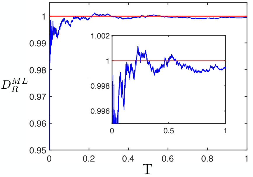
We adimensionalized time using the rotational diffusion coefficient $D_{R}$, and simulated trajectories with different duration $T$. The (dimensionless) time interval between two sampling events is fixed as $\Delta t=10^{-6}$. To test the convergence of the method, we compute the diffusion coefficient $D_{R}^{ML}$, using Eq (13), for trajectories of different duration. In Fig. 3, we illustrate the convergence of the estimated value $D_{R}^{ML}$ towards the prescribed value $D_{R}^{*}=1$ as the length of the trajectory increases. For instance, we find a value of $D_{R}^{ML}$ very close to 1, i.e $D_{R}^{ML}=0.9994$, at $T=1$.

In this case we simulate Eqs. (1) and (II.1) with a flow profile of the form $\mathbf{v}^{F}(\mathbf{r})=\dot{\gamma}z\mathbf{e_{x}}$, where $\dot{\gamma}$ is the shear rate. As before, simulations are performed using dimensionless variables. Time is adimensionalized by the inverse of the shear rate, so the relevant dimensionless, diffusion-related quantity to be estimated in this case is is the Péclet number, $Pe=\dot{\gamma}/D_{R}$. Note that the Péclet number can be directly estimated using Eq. (13), since it is just a rescaling of $\tilde{\mathcal{N}}_{R}$ by the known quantities $\dot{\gamma}$ and $f$, $Pe=(\dot{\gamma}/f)\tilde{\mathcal{N}}_{R}$.

We simulate trajectories for a vector $(\beta^{*},Pe^{*})=(0.9,100)$. To test the convergence of the ML method, we generate a set of trajectories of different duration $T$ with randomly chosen initial positions and orientations. In Fig. 4, we present the results of shear flow simulations. For a given trajectory length $T$, the estimated value of the parameters ($\beta^{ML}$ in Fig. 4(a) and $Pe^{ML}$ in Fig. 4(b)) are scattered around $Pe^{*}$ and $\beta^{*}$. This scattering is linked to the randomness encoded in the noise and the initial orientations. The average value of the estimations over all trajectories of the same length (dark blue points) is very close to the input value of the simulations. On average, even for short trajectories, the ML method gives a good estimation of the parameters. For instance, for a trajectory of duration $T=10$, the averaged estimated parameter differ only by $1\%$ from the input values. As $T$ increases, the scattering of the estimators decreases and our estimators become accurate for individual trajectories. Moreover, the standard deviation of the estimated parameters is bounded by the uncertainties computed using the expressions Eq. (15) and Eq. (16) and decays as $N^{-1/2}$.

We now test the method on a Poiseuille flow profile. Here we consider a flow confined between two infinite plates separated by a vertical distance $h$, so that the velocity profile is given by $\mathbf{v}^{F}(\mathbf{r})=\frac{4U_{m}}{h}z\Big(1-\frac{z}{h}\Big)\mathbf{e_{x}}$. $U_{m}$ denotes the maximal flow velocity at the middle of the Poiseille flow ($z=h/2$). We also work with dimensionless variables in this case, so that lengths and time are adimensionlalized using $h$ and the maximum shear rate $\dot{\gamma}_{W}=\frac{4U_{m}}{h}$, respectively. In addition to $\beta$, the relevant dimensionless parameter is again the Péclet number, $Pe=\frac{\dot{\gamma}_{W}}{D_{R}}$. We simulate trajectories for a vector: $(\beta^{*},Pe^{*})=(0.9,100)$ and different durations $T$ with the additional constraint that the simulation ends when the particle hits the surfaces (located in z=0 and z=1). For instance, for the parameters used in the Fig.5, it is difficult to have trajectories longer than T=50.

For a given $T$, the estimators are scattered around the input values. As $T$ increases the scattering decreases. The estimator $Pe^{ML}$ remains very good, both on average (less than $2\%$ of error) and for individual trajectories (less than $10\%$ of error), even for trajectories with durations as short as $T=1$. The estimator $\beta^{ML}$ is not as good as in the shear flow, but we still have an average estimated value within a $10\%$ of the input one. The standard deviation of the estimated values are still bounded by the expressions Eq. (15) and Eq. (16) and still decrease as $N^{-1/2}$. Our estimators can be further improved by computing errors up to $O(N^{-1})$ to compensate for the shorter tracks. This will be discussed in more detail elsewhere.

References

- Manzo and Garcia-Parajo (2015) C. Manzo and M. F. Garcia-Parajo, Rep. Prog. Phys. 78, 124601 (2015).
- Sarfati et al. (2017) R. Sarfati, J. Bławzdziewicz, and E. R. Dufresne, Soft Matter 13, 2174 (2017).
- Seyrich et al. (2018) M. Seyrich, Z. Alirezaeizanjani, C. Beta, and H. Stark, New J. Phys. 20, 103033 (2018).
- Pérez García et al. (2018) L. Pérez García, J. Donlucas Pérez, G. Volpe, A. V. Arzola, and G. Volpe, Nat. Commun. 9, 5166 (2018).
- Frishman and Ronceray (2020) A. Frishman and P. Ronceray, Phys. Rev. X 10, 021009 (2020).
- Lanoiselée and Grebenkov (2016) Y. Lanoiselée and D. S. Grebenkov, Phys. Rev. E 93, 052146 (2016).
- Lanoiselée and Grebenkov (2017) Y. Lanoiselée and D. S. Grebenkov, Phys. Rev. E 96, 022144 (2017).
- Gardel et al. (2005) M. L. Gardel, M. T. Valentine, and D. A. Weitz, in Microscale Diagnostic Techniques, edited by K. Breuer (Springer, Oxford, 2005) pp. 1–50.
- Abou and Gallet (2004) B. Abou and F. m. c. Gallet, Phys. Rev. Lett. 93, 160603 (2004).
- Puertas and Voigtmann (2014) A. M. Puertas and T. Voigtmann, J. Phys. Condens. Matter 26, 243101 (2014).
- Wirtz (2009) D. Wirtz, Annu. Rev. Biophys. 38, 301 (2009).
- Struntz and Weiss (2018) P. Struntz and M. Weiss, Phys. Chem. Chem. Phys. 20, 28910 (2018).
- Wu and Libchaber (2000) X.-L. Wu and A. Libchaber, Phys. Rev. Lett. 84, 3017 (2000).
- Miño et al. (2011) G. Miño, T. E. Mallouk, T. Darnige, M. Hoyos, J. Dauchet, J. Dunstan, R. Soto, Y. Wang, A. Rousselet, and E. Clement, Phys. Rev. Lett. 106, 048102 (2011).
- Jeanneret et al. (2016) R. Jeanneret, D. O. Pushkin, V. Kantsler, and M. Polin, Nat. Commun. 7, 12518 (2016).
- Chen et al. (2007) D. T. N. Chen, A. W. C. Lau, L. A. Hough, M. F. Islam, M. Goulian, T. C. Lubensky, and A. G. Yodh, Phys. Rev. Lett. 99, 148302 (2007).
- Miño et al. (2013) G. L. Miño, J. Dunstan, A. Rousselet, E. Clément, and R. Soto, J. Fluid Mech. 729, 423 (2013).
- Kasyap et al. (2014) T. V. Kasyap, D. L. Koch, and M. Wu, Phys. Fluids 26, 081901 (2014).
- Marini Bettolo Marconi and Maggi (2015) U. Marini Bettolo Marconi and C. Maggi, Soft Matter 11, 8768 (2015).
- Fodor et al. (2016) E. Fodor, C. Nardini, M. E. Cates, J. Tailleur, P. Visco, and F. van Wijland, Phys. Rev. Lett. 117, 038103 (2016).
- Dabelow et al. (2019) L. Dabelow, S. Bo, and R. Eichhorn, Phys. Rev. X 9, 021009 (2019).
- Burkholder and Brady (2019) E. W. Burkholder and J. F. Brady, J. Chem. Phys. 150, 184901 (2019).
- Katuri et al. (2016) J. Katuri, K. D. Seo, D. S. Kim, and S. Sánchez, Lab Chip 16, 1101 (2016).
- Baraban et al. (2013) L. Baraban, S. M. Harazim, S. Sanchez, and O. G. Schmidt, Angew. Chem. Int. Ed. 52, 5552 (2013).
- Palacci et al. (2015) J. Palacci, S. Sacanna, A. Abramian, J. Barral, K. Hanson, A. Y. Grosberg, D. J. Pine, and P. M. Chaikin, Sci. Adv. 1 (2015).
- Junot et al. (2019) G. Junot, N. Figueroa-Morales, T. Darnige, A. Lindner, R. Soto, H. Auradou, and E. Clément, EPL 126, 44003 (2019).
- Thapa et al. (2018) S. Thapa, M. A. Lomholt, J. Krog, A. G. Cherstvy, and R. Metzler, Phys. Chem. Chem. Phys. 20, 29018 (2018).
- Masson et al. (2012) J.-B. Masson, G. Voisinne, J. Wong-Ng, A. Celani, and M. Vergassola, Proc. Natl. Acad. Sci. U.S.A. 109, 1802 (2012).
- Martin et al. (1973) P. C. Martin, E. D. Siggia, and H. A. Rose, Phys. Rev. A 8, 423 (1973).
- de Dominics (1976) C. de Dominics, J. Phys. (Paris) Colloq. 37, C1 (1976).
- Janssen (1976) H.-K. Janssen, Z. Phys. B 23, 377 (1976).
- Newey and McFadden (1994) W. K. Newey and D. McFadden (Elsevier, 1994) pp. 2111 – 2245.
- Perrin (1934) F. Perrin, J. Phys. Radium 5, 497 (1934).
- Perrin (1936) F. Perrin, J. Phys. Radium 7, 1 (1936).
- Son et al. (2013) K. Son, J. S. Guasto, and R. Stocker, Nat. Phys. 9, 494 (2013).
- Spöring et al. (2018) I. Spöring, V. A. Martinez, C. Hotz, J. Schwarz-Linek, K. L. Grady, J. M. Nava-Sedeño, T. Vissers, H. M. Singer, M. Rohde, C. Bourquin, H. Hatzikirou, W. C. K. Poon, Y. S. Dufour, and M. Erhardt, PLOS Biology 16, 1 (2018).
- Marcos et al. (2012) Marcos, H. C. Fu, T. R. Powers, and R. Stocker, Proc. Natl. Acad. Sci. U.S.A. 109, 4780 (2012).
- Darnige et al. (2017) T. Darnige, N. Figueroa-Morales, P. Bohec, A. Lindner, and E. Clément, Rev. Sci. Instrum. 88, 055106 (2017).