Human Motion Tracking by Registering an Articulated Surface to 3-D Points and Normals

One convenient way to describe 3-D ellipsoids is to use an implicit equation and to embed the 3-D Euclidean space into the 3-D projective space. This yields a 4$\times$4 full-rank symmetric matrix Q:

where $\mbox{\bf D}=\mbox{Diag}\>[a^{-2},b^{-2},c^{-2}]$ is a $3\times$3 diagonal matrix, R is a $3\times 3$ rotation matrix and $t$ is a 3-D translation vector. In practice $b=c$ and we choose $a\geq b$. We denote by $X$ the homogeneous coordinates of a point $x$ lying onto the surface of the ellipsoid, $\mbox{\boldmath$X$}^{\top}\mbox{\bf Q}\mbox{\boldmath$X$}=0$. The adjoint matrix $\mbox{\bf Q}^{\star}=\mbox{\bf Q}^{-\top}$ defines the dual ellipsoid. The family $P$ of planes which are tangent to the ellipsoid Q satisfy the constraint $\mbox{\boldmath$P$}^{\top}\mbox{\bf Q}^{-1}\mbox{\boldmath$P$}=0$ since $\mbox{\bf Q}^{\top}=\mbox{\bf Q}$. We denote by $p$ the 3-D vector which is orthogonal to the plane $P$ (therefore $p$ is normal to the ellipsoid at point $x$): $\mbox{\boldmath$p$}=\overline{\mbox{\bf Q}}\mbox{\boldmath$x$}+\mbox{\boldmath$q$}$, where the notations of eq. (1) are used.

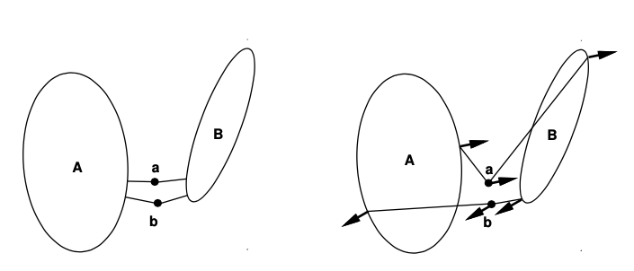
The algebraic distance from a 3-D point $Y$ to the surface of an ellipsoid was used in [12], defined by $q(\mbox{\boldmath$Y$})=\mbox{\boldmath$Y$}^{\top}\mbox{\bf Q}\mbox{\boldmath$Y$}$. The value of $q$ varies from $-1$ at the center of the ellipsoid, to $0$ on its surface, and then to $+\infty$ outside the ellipsoid as the point is farther away from the surface. The Euclidean distance from a point to an ellipsoid requires to solve a six-degree polynomial. In [6] an approximation of the Euclidean distance is used, i.e, a pseudo-Euclidean distance, as shown on Figure 1.

An observation will be refered to as a 3-D datum and consists of both a 3-D point and a 3-D vector. We define a metric between such a 3-D datum and an ellipsoid as follows. Let $\mbox{\boldmath$Y$}^{\top}=(\mbox{\boldmath$y$}^{\top}\;1)$ be the homogeneous coordinates of an observed point, and let $n$ be a 3-D observed vector. An observation or a 3-D datum is denoted by ${\cal{Y}}=(\mbox{\boldmath$y$},\mbox{\boldmath$n$})$. We seek an ellipsoid point $\mbox{\boldmath$X$}=(\mbox{\boldmath$x$}^{\top}\;1)$ under the constraint that the vector $p$ (normal to the ellipsoid at $x$) is aligned with $n$, e.g. Figure 1. In other words, we seek an association between ${\cal{X}}=(\mbox{\boldmath$x$},\mbox{\boldmath$p$})$ and ${\cal{Y}}=(\mbox{\boldmath$y$},\mbox{\boldmath$n$})$. Figure 2 compares the distance used in this paper with the Euclidean distance from a point to an ellipsoid.

Let $d_{{\cal{E}}}({\cal{Y}},{\cal{X}})$ be the Euclidean distance from the datum-point $y$ to the ellipsoid-point $x$ under the constraint that the datum-vector $n$ and the ellipsoid-vector $p$ are parallel:

where $\|\mbox{\boldmath$a$}\|_{2}$ denotes the Euclidean norm. We seek a solution for $x$ under the constraints that $p$ and $n$ are parallel and yield the same orientation. Using eq. (1) we obtain the following set of constraints:

From eq. (4) we obtain $\mbox{\boldmath$x$}=\overline{\mbox{\bf Q}}\;^{-1}\left(\lambda\mbox{\boldmath$n$}-\mbox{\boldmath$q$}\right)$. By substitution in eq. (3) we obtain two solutions for $\lambda$. From $\mbox{\boldmath$p$}^{\top}\mbox{\boldmath$n$}>0$ we have $\lambda>0$ and $\lambda=(\mbox{\boldmath$n$}^{\top}\mbox{\bf R}\mbox{\bf D}^{-1}\mbox{\bf R}^{\top}\mbox{\boldmath$n$})^{-1/2}$. Therefore, the point onto the ellipsoid where its normal $p$ is aligned with $n$ is given by:

It will be convenient to use the Mahalanobis distance:

Articulated motion has a long history in mechanics, biomechanics, robotics, and computer vision. A human body can be described by a number of open kinematic chains that share a common root. Such an open chain is composed of a number of rigid objects and two consecutive rigid objects in the chain are mechanically linked to form a joint. Rotational (or spherical) joints are the most convenient representations and they are well suited for human body modeling. Each such joint may have one, two, or three rotational degrees of freedom. Therefore, within such a chain, a body part Q is linked to a root body part $\mbox{\bf Q}_{r}$ through a constrained motion, i.e., a kinematic chain with a number of rotational degrees of freedom. Since each joint may have several degrees of freedom, the total number of rotational parameters of a chain is larger than the number of rigid parts composing the chain. Moreover, the root body part undergoes a free motion itself, i.e., a rigid displacement with up to six degrees of freedom: three rotations and three translations.

Therefore the motion of a body-part (or ellipsoid) Q is composed of the root’s free motion followed by the chain’s constrained motion. We will denote the motion of Q by the 4$\times$4 homogeneous matrix T which in turn is parameterized by the joint and free-motion parameter vector $\Lambda$:

A complete human-body model may be described with five kinematic chains that share a common root body-part. In this paper we use the following simplified human-body model. There are 14 body parts and 11 joints (2 ankles, 2 knees, 2 hips, 2 elbows, 2 shoulders, and a neck) with $22$ rotational degrees of freedom (there are two degrees of freedom for each joint). We also consider 3 rotations and 3 translations for the free motion. Hence, there is a total of 26 degrees of freedom.

As detailed above, body parts are described by one or several ellipsoids: The feet and the thighs are described by two ellipsoids, the torso is described by three ellipsoids, and all the other body parts are described by a single ellipsoid, hence there are 21 ellipsoids, e.g., Figure 3. The body parts are denoted by $\mbox{\bf Q}_{p},1\leq p\leq P$, where, for convenientce, $\mbox{\bf Q}_{1}$ corresponds to the common root body part.

In addition to using a collection of kinematically linked ellipsoids, we will fuse them in order to define a smooth surface $\mathcal{S}$ over the entire body. This surface will be described by the implicit equation $f(\mbox{\boldmath$y$})=C$ with $C=1$. The contribution of an ellipsoid $\mbox{\bf Q}_{p}$ is defined by:

where $d_{\mathcal{M}}$ is the Mahalanobis distance from $y$ to the ellipsoid defined by eq. (6), the point $\mbox{\boldmath$x$}_{p}$ lies onto the ellipsoid, and $\nu_{p}^{2}$ is a parameter that tunes the spatial influence of the ellipsoid.

An implicit surface is defined as a level set of the following implicit function which is the fusion (or blending) of $P$ ellipsoids verifying:

The class of implicit surfaces defined as above, i.e., $\mbox{\boldmath$y$}\in\mathcal{S}\Leftrightarrow f(\mbox{\boldmath$y$})=C$, has successfully been used in computer graphics and in computer vision in conjunction with the algebraic distance [12] and with the pseudo-Euclidean distance [6]. Within this paper we extend this concept to the distance defined above. As it will be detailed below, this is well suited to cast the problem of implicit surface fitting into the framework of maximum likelihood in the presence of outliers.

In order to track articulated objects, the task at hand consists of fitting the articulated implicit surface just described to a set of observations. For this purpose, we first define a distance from a set of observations to the implicit surface. We have to solve the equation $f(\mbox{\boldmath$y$})=1$, where $y$ is, as before, an observed 3-D point. One may notice that the first order Taylor expansion of $\ln a$ at $a=1$ is: $\ln a=a-1+O(a^{2})$. We retain the following approximation of the distance from a set of $I$ observations to the articulated implicit surface formed by $P$ ellipsoids and parameterized by the kinematic variables $\Lambda$:

where:

For convenience, we set $\nu=\nu_{1}=\ldots=\nu_{P}$. The notation $\mbox{\boldmath$x$}_{ip}$ means that the 3-D point $x$ lies on ellipsoid $p$ and is associated with observation $i$. It is worthwhile to notice that, whenever a set of observations is closed to one of the ellipsoids, the distance function is strictly equal to the sum of Mahalanobis distances from each such observation to the ellipsoid.

In this section we introduce a probabilistic interpretation of eq. (10). For this purpose we denote by $z_{i}$ a random variable that assigns an observation $i$ to an ellipsoid $p$, namely the notation $z_{i}=p$ means that the $i^{th}$ observation is assigned to the $p^{th}$ ellipsoid. There are as many hidden variables $z_{i}$ as observations: $i\in\{1,\ldots,I\}$. The set of all the hidden variables is denoted by $\mathcal{Z}=\{z_{1},\ldots,z_{I}\}$.

The likelihood of an observed 3-D point, given its assignment to an ellipsoid and given an observed 3-D normal, is drawn from a Gaussian distribution:

In practice the data are corrupted by noise and by errors and therefore there are observations which should not be assigned to an ellipsoid. For this reason we introduce an outlier class denoted by $P+1$, and we assume that the likelihood of an observation given that is classified as an outlier is a uniform distribution over the volume $V$ of the working space:

Therefore, one can write the likelihood of an observation as a mixture of $P$ Gaussian components and one uniform component:

The notation:

denotes the priors, the proportions, or the mixing parameters, and they obey the obvious constraint $\sum_{p=1}^{P+1}\pi_{p}=1$. Notice that this prior probability depends on the observed vector $\mbox{\boldmath$n$}_{i}$. In this paper we do not treat these observed vectors as random variables. By assuming independent and identically distributed observations one can write the joint likelihood of all the observations as:

Using Bayes’ formula and the equations above, the negative log-likelihood writes:

Notice that there is a strong analogy between eqs. (10) and (15): the former is a distance between a set of $I$ observations and an articulated implicit surface while the latter is the joint likelihood of the same observation set, where the likelihood is a mixture of $P$ normal distributions plus a uniform distribution that captures the bad observations. This analogy will be exploited in the next section in order to cast the estimation of the kinematic parameters in the framework of maximum likelihood with hidden variables via the EM algorithm.

We used an animation package to build a human body, to simulate various human motions, and to render image silhouettes. The simulator uses its own shape representation, that is different than ours, but it allows the user to define her/his own kinematic model. Therefore we used the same kinematic model with the same number of degrees of freedom as the one described in section II-B. Nevertheless, we have not attempted to finely tune the shape parameters of our model to the simulated data. We simulated a setup composed of seven calibrated cameras. Sequences of image silhouettes were generated from the 3-D model and rendered with the cameras’ parameters. We computed 3-D points and normals from these silhouettes and then we applied our method to these data sets. The articulated-motion parameters were recovered using our tracker. In order to assess the merits of the data-to-model fitting process, we added 20% of outliers uniformly distributed in the volume of the working space. These simulations allowed us to (i) assess the quality of the tracker with respect to ground-truth joint trajectories, (ii) analyse the behavior of the method in the presence of various perturbations that alter the quality of the data, (iii) quantify the merit of using both 3-D points and normals instead of using only points, and (iv) determine the optimal number of observations needed for reliable estimation of articulated motion.

We simulated a running sequence that involves both kinematic and free-motion parameters. The graphs of Figure 4 illustrate the average error between the simulated angle values and their estimated values (measured in radians) for the kinematic parameters but not for the free-motion parameters. The first graph compares the ground-truth (simulated) joint trajectories of the left knee and of the right elbow (dashed curve) with the trajectories estimated with our method (solid curve) over 100 frames. The second graph illustrates the behavior of the method in the presence of silhouette noise. The results of using both 3-D points and normals (dashed curve) are plotted against the results obtained using 3-D points and the algebraic distance (solid line). The relative large error corresponds to the fact that the shape model used by the animation package is not the same as our shape model. Hence, there is a systematic offset between the ground-truth kinematic parameters and the estimated parameters.

The third graph shows the average angle error as a function of the number of frames per second. The last graph shows the influence of the number of observations, where the latter varies from 50 to 550. The average angle error drops as the number of observations increases and our method (dashed) performs better than using 3-D points alone (solid). From all these experiments one may conclude that tracking is improved when both points and normals are used instead of just points.

The experimental data that we used for validating the human motion tracker was gathered with six calibrated and finely synchronized cameras. Each camera delivers 780$\times$580 color images at 28 frames per second with a synchronization accuracy within 1 mili-second. The figures below show these image sequences sampled at 14 frames per second.

We applied articulated human motion tracking to two multiple-image sequences, the taekwendo sequence shown on Figure 5 and the leaning sequence shown of Figure 7. The first data set is composed of 6$\times$700 frames while the second one is composed of 6$\times$200 frames. We used the same body-part dimensions for the two characters. One may notice that the silhouettes have holes and missing pieces, which results in the presence of 3-D outliers. The top row in Figure 6 shows the 3-D points and normals that were reconstructed from the imperfect silhouettes; The middle row shows the articulated implicit surface resulting from application of our method, while the bottom row shows the same surface resulting from application of our method in conjunction with the algebraic distance. Obviously, in this last case, there is a discrepancy between the data and the fitted model: the recovered motion of the right feet and the right thigh are incorrect. Similarly, figure 7 shows a sample of the leaning sequence, the corresponding silhouettes, and the fitted model using the proposed method.

References

- [1] C.M. Bishop. Pattern Recognition and Machine Learning. Springer, 2006.
- [2] E. Boyer and J-S. Franco. A hybrid approach for computing visual hulls of complex objects. In Proceedings of the IEEE Conference on Computer Vision and Pattern Recognition, pages 695–701, Madison, Wisconsin, USA, June 2003. IEEE Computer Society Press.
- [3] G.J. Brostow, I.A. Essa, D. Steedly, and V. Kwatra. Novel skeletal representation for articulated creatures. In European Conference on Computer Vision, pages Vol III: 66–78, 2004.
- [4] K.-M. Cheung, S. Baker, and T. Kanade. Shape-from-silhouette across time part ii:applications to human modeling and markerless motion. International Journal of Computer Vision, 63(3):225–245, 2005.
- [5] D. Demirdjian. Combining geometric- and view-based approaches for articulated pose estimation. In European Conference on Computer Vision, pages Vol III: 183–194, 2004.
- [6] G. Dewaele, F. Devernay, R. Horaud, and F. Forbes. The alignment between 3-d data and articulated shapes with bending surfaces. In Proceedings of the 9th European Conference on Computer Vision, Graz, Austria, volume III of LNCS, pages 578–591. Springer, May 2006.
- [7] C. Fraley and A. E. Raftery. Model-based clustering, discriminant analysis, and density estimation. Journal of the American Statistical Association, 97:611–631, 2002.
- [8] J-S. Franco, M. Lapierre, and E. Boyer. Visual shapes of silhouette sets. In Proceedings of the 3rd International Symposium on 3D Data Processing, Visualization and Transmission, Chapel Hill (USA), 2006.
- [9] S. Ilic, M. Salzmann, and P. Fua. Implicit meshes for effective silhouette handling. International Journal of Computer Vision, 72(2):159 – 178, 2007.
- [10] D. Knossow, R. Ronfard, and R. Horaud. Human motion tracking with a kinematic parameterization of extremal contours. International Journal of Computer Vision, 2008. To appear.
- [11] B. Luo and E.R. Hancock. Structural graph matching using the EM algorithm and singular value decomposition. IEEE Transactions on Pattern Analysis and Machine Intelligence, 23(2001):1120–1136, October 2001.
- [12] R. Plankers and P. Fua. Articulated Soft Objects for Multi-View Shape and Motion Capture. IEEE Transactions on Pattern Analysis and Machine Intelligence, 25(9):1182–1187, 2003.
- [13] J. Starck and A. Hilton. Model-based multiple view reconstruction of people. In IEEE International Conference on Computer Vision, October 2003.
- [14] W.M. Wells III. Statistical approaches to feature-based object recognition. International Journal of Computer Vision, 28(1/2):63–98, 1997.