- phase transition of zirconium predicted by on-the-fly machine-learned force field
Abstract
The accurate prediction of solid-solid structural phase transitions at finite temperature is a challenging task, since the dynamics is so slow that direct simulations of the phase transitions by first-principles (FP) methods are typically not possible. Here, we study the - phase transition of Zr at ambient pressure by means of on-the-fly machine-learned force fields. These are automatically generated during FP molecular dynamics (MD) simulations without the need of human intervention, while retaining almost FP accuracy. Our MD simulations successfully reproduce the first-order displacive nature of the phase transition, which is manifested by an abrupt jump of the volume and a cooperative displacement of atoms at the phase transition temperature. The phase transition is further identified by the simulated x-ray powder diffraction, and the predicted phase transition temperature is in reasonable agreement with experiment. Furthermore, we show that using a singular value decomposition and pseudo inversion of the design matrix generally improves the machine-learned force field compared to the usual inversion of the squared matrix in the regularized Bayesian regression.
I Introduction
Because of widespread applications in nuclear, chemical, and manufacturing process industries Northwood 1985; Kalavathi and Kumar Bhuyan 2019, zirconium has stimulated extensive interest in fundamental research aiming to clarify the underlying mechanisms responsible for the phase transitions and phase diagram from both experiment and theory Vogel and Tonn 1931; Fisher and Renken 1964; Olinger and Jamieson 1973; Sikka et al. 1982; Xia et al. 1990; *Xia_PRB1991; Song and III 1995; Zhao et al. 2005; Zhang et al. 2005; Liu et al. 2008; Akahama et al. 1991; *Akahama_Exp1992; Ostanin and Trubitsin 1998; Stavrou et al. 2018; Burgers 1934; Petry 1991; Ahuja et al. 1993; Greeff 2005; Schnell and Albers 2006; Souvatzis et al. 2011; Chen et al. 1985; Zong et al. 2018; Souvatzis et al. 2008; Qian and Yang 2018; Stassis et al. 1978; Ye et al. 1987; Heiming et al. 1991; Hu et al. 2011; Willaime and Massobrio 1989; Zong et al. 2020; Hellman et al. 2011. Upon cooling the melt, Zr solidifies to a body-centred cubic (bcc) structure (the phase) and undergoes a phase transformation to a hexagonal close-packed (hcp) structure (the phase) at a temperature lower than 1136 K at zero pressure Vogel and Tonn 1931 and at lower temperatures under pressure Zhang et al. 2005. With increasing pressure, the hcp phase transforms into another hexagonal but not close-packed structure (the phase) Olinger and Jamieson 1973; Sikka et al. 1982; Xia et al. 1990; Song and III 1995; Zhao et al. 2005; Zhang et al. 2005; Liu et al. 2008. Under further increased pressure, the phase transforms to the phase Xia et al. 1990; Zhang et al. 2005. The experimentally estimated -- triple point is at 4.9 GPa and 953 K Zhang et al. 2005.
To understand the microscopic mechanism of the bcc-hcp phase transition of Zr, Burgers Burgers 1934 proposed that the transition can be divided into two processes. As illustrated in Fig. 1, the bcc phase first undergoes a long wavelength shear in the [11] direction along the (112) plane (or equivalently in the [11] direction along the (2) plane), which squeezes the bcc octahedron to the hcp one, thereby changing the angle between the [11] and [11] directions from 109.5∘ to 120∘ Burgers 1934; Petry 1991. Then, the neighboring (011) planes of the bcc phase experience a shuffle along opposite [01] directions with a displacement of Burgers 1934; Petry 1991 [compare Figs. 1(b) and (c)]. The shuffle originates from displacements along the zone-boundary -point phonon of the branch in the [110] direction Burgers 1934; Petry 1991. The transition belongs to the martensitic transformations, is of first order and displacive, and adopts the definite orientational crystallographic relation (011)β //(0001)α and [11]β //[20]α Burgers 1934.
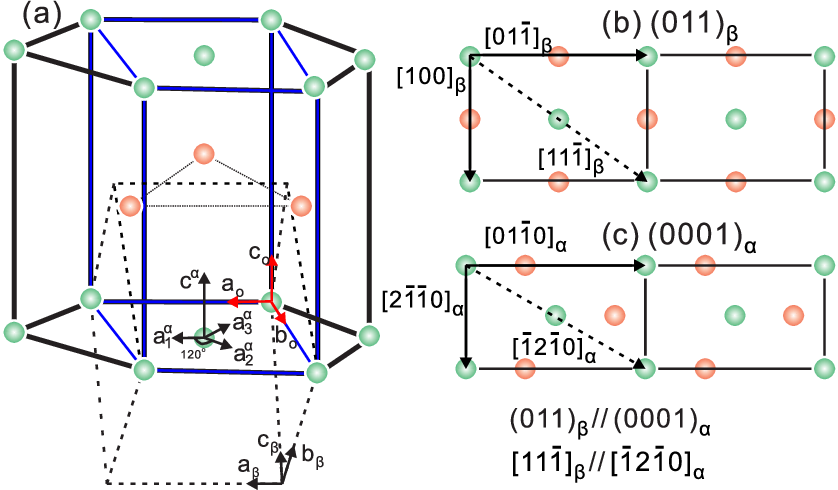
The Burgers mechanism was later confirmed by Willaime and Massobrio Willaime and Massobrio 1989 using classic molecular-dynamics (MD) simulations based on a semi-empirical tight-binding interatomic potential Willaime and Massobrio 1991, giving valuable insight on the temperature-induced hcp-bcc phase transition of Zr from an atomistic point of view. However, their predicted phase transition temperature deviated by nearly 800 K from the experimental value, since their potential was fitted to the hcp Zr phase only Willaime and Massobrio 1989. By including zero-temperature as well as high-temperature properties of both hcp and bcc Zr phases in the fitting procedure, Mendelev and Ackland Mendelev and Ackland 2007 developed an embedded-atom interatomic potential that predicted a reasonable hcp-bcc transition temperature. Some residual dependency on the target properties used in the fitting, however, remained. Furthermore, these physics-based semi-empirical potentials, in general, suffer from limited accuracy and are not very flexible, because of their rather simple analytical form. This cannot capture the properties of structures over a large phase space.
Machine learning (ML) based regression techniques Behler and Parrinello 2007; Bartók et al. 2010; Behler 2017; Botu et al. 2017; De et al. 2016; Schmidt et al. 2019 have recently emerged as a promising tool to construct interatomic potentials. Their advantage is that they are entirely data-driven and do not assume any specific functional form. Most machine-learned force fields (MLFF) try to learn the potential energy surface as well as its derivatives by finding a map from the local atomic environments onto local energies. Typically, energies, forces, and stress tensors that are calculated by first-principles (FP) techniques are fitted. Using the kernel ridge regression method, Zong et al. generated an interatomic potential that successfully reproduced the phase diagram of Zr Zong et al. 2018 and uncovered the nucleation mechanism for the shock-induced hcp-bcc phase transformation in hcp-Zr Zong et al. 2020. Using the Gaussian approximation potential model Bartók et al. 2010; Bartók et al. 2013, Qian and Yang Qian and Yang 2018 studied the temperature-induced phonon renormalization of bcc Zr and clarified the origin of its instability at low temperature. However, for the hereto employed ML methods, construction of suitable training structures is a fairly time-consuming trial and error process based on intuition. The thus obtained training datasets are normally huge and might contain unnecessary structures outside the phase space of interest. This can even reduce the accuracy of the generated ML potential. Furthermore, the generated ML potential showed only fair agreement with phonon frequencies and elastic constants calculated using density functional theory (DFT).
To reduce human intervention, on-the-fly machine learning schemes Li et al. 2015; Jacobsen et al. 2018; Jinnouchi et al. 2019a provide an elegant solution. These generate the force fields automatically during FP MD simulations while exploring potentially a large phase space. In particular, Jinnouchi et al. Jinnouchi et al. 2019a; Jinnouchi et al. 2019b suggested using the predicted Bayesian error to judge whether FP calculations are required or not. In this manner, usually more than 98% of the FP calculations are bypassed during the training, significantly enhancing the sampling of the configuration space and the efficiency of the force field generation Jinnouchi et al. 2019a. This method has been successfully applied to the accurate and efficient prediction of entropy-driven phase transitions of hybrid perovskites Jinnouchi et al. 2019a, melting points Jinnouchi et al. 2019b, as well as chemical potentials of atoms and molecules Jinnouchi et al. 2020a.
In this work, we attempt to revisit the hcp-bcc phase transition of Zr at ambient pressure by using the on-the-fly MLFF method developed by Jinnouchi et al. Jinnouchi et al. 2019a; Jinnouchi et al. 2019b. Almost without any human intervention, our generated MLFF successfully reproduces the phonon dispersions of both the hcp and bcc phases at 0 K as well as the first-order displacive nature of the phase transition manifested by an abrupt jump of the volume and cooperative movement of atoms at the phase transition temperature. This confirms the Burgers mechanism Burgers 1934. The phase transition is further confirmed by the simulated x-ray powder diffraction. Moreover, we demonstrate that using a singular value decomposition for the regression overall improves the accuracy of the MLFF compared to the regularized Bayesian regression.
II Method
For a comprehensive description of the on-the-fly MLFF generation implemented in the Vienna Ab initio Simulation Package (VASP), we refer to Ref. Jinnouchi et al. 2019b. A perspective article on this method can be found in Ref. Jinnouchi et al. 2020b. Here, we just summarize the most important aspects of the underlying MLFF techniques.
As in many MLFF methods Behler and Parrinello 2007; Bartók et al. 2010; Behler 2017; Botu et al. 2017; Bartók et al. 2013; Seko et al. 2014; Shapeev 2016; Glielmo et al. 2018; Faber et al. 2018; De et al. 2016; Schmidt et al. 2019, the potential energy of a structure with atoms is approximated as a summation of local atomic potential energies
| (1) |
where is described as a functional of the two-body () and three-body () distribution functions,
| (2) |
The two-body distribution function is defined as the probability to find an atom at a distance from atom Jinnouchi et al. 2019b; Jinnouchi et al. 2020c
| (3) |
where () is the three-dimensional atom distribution function around the atom defined as
| (4) | ||||
Here, is the likelihood to find atom at position relative to atom , is a cutoff function that smoothly eliminates the contribution from atoms outside a given cutoff radius , and is a smoothed -function. The three-body distribution function is defined as the probability to find an atom at a distance from atom and another atom at a distance from atom spanning the angle between them. It is defined as Jinnouchi et al. 2020c
| (5) |
It should be noted that the definition of in Eq. (5) is free of two-body components and the importance of the two- and three-body descriptors can thus be separately tuned. To distinguish from the power spectrum Bartók et al. 2013, we denote these descriptors as the separable descriptors. For more discussions on the difference between the separable descriptors and the power spectrum, we refer to Ref. Jinnouchi et al. 2020c.
In practice, and are discretized in a suitable basis and represented by a descriptor vector collecting all two- and three-body coefficients Jinnouchi et al. 2020c. Therefore, the functional in Eq. (2) becomes a function of Jinnouchi et al. 2020c
| (6) |
For the functional form of , a kernel based approach is used Bartók et al. 2013. Specifically, using the algorithm of data selection and sparsification Jinnouchi et al. 2019b, atoms are chosen from a set of reference structures generated by FP MD simulations and the atomic distributions surrounding the selected atoms are mapped onto the descriptors . The function is then approximated by the linear equation of coefficients
| (7) |
where the kernel function is a nonlinear function that is supposed to quantify the degree of similarity between a local configuration of interest and the reference configuration . Here, a polynomial function is used Bartók et al. 2013; Jinnouchi et al. 2020c. This introduces nonlinear mixing of purely two- and three-body descriptors, which was found to be important for an accurate and efficient description of the potential energy surfaces Jinnouchi et al. 2020c.
From Eq. (7), the total energy, forces and stress tensors of any structure can be obtained as linear equations of the coefficients . In a matrix-vector representation, it can be expressed as
| (8) |
where is a vector collecting the FP energy, forces, and stress tensors for the given structure of atoms, in total, components. is a matrix. The first line of the matrix is comprised of , the subsequent lines consist of the derivatives of the kernel with respect to the atomic coordinates, and the final six lines consist of the derivatives of the kernel with respect to the unit cell coordinates Jinnouchi et al. 2019b. is a vector collecting all coefficients . The generalized linear equation containing all reference structures is given by
| (9) |
Here, is a super vector collecting all FP energies, forces, and stress tensors for all reference structures and similarly, is the design matrix comprised of matrices for all reference structures Jinnouchi et al. 2019b. Based on Bayesian linear regression (BLR), the optimal coefficients are determined as Jinnouchi et al. 2019b; Bishop 2006
| (10) |
where is the variance of the uncertainty caused by noise in the training datasets, and is the variance of the prior distribution Jinnouchi et al. 2019b. The parameters and are obtained by maximizing the evidence function Jinnouchi et al. 2019b.
Having obtained the optimal coefficients , the energy, forces, and stress tensors for any given structure can be predicted by , and the uncertainty in the prediction is estimated as the variance of the posterior distribution Jinnouchi et al. 2020b
| (11) |
It is found that the square root of the second term in Eq. (11) resembles the real error remarkably well Jinnouchi et al. 2019b and thus provides a reliable measure of the uncertainty. This is the heart of the on-the-fly MLFF algorithm. Armed with a reliable error prediction, the machine can decide whether new structures are out of the training dataset or not by using state-of-the-art query strategies Jinnouchi et al. 2019b. Only if the machine finds the need to update the training dataset with the new structures, then FP calculations are carried out. Otherwise, the predicted energy, forces, and stress tensors by the yet available MLFF are used to update the atomic positions and velocities. In this manner, most of the FP calculations are bypassed during training runs and simulations are in general accelerated by several orders of magnitude while retaining almost FP accuracy Jinnouchi et al. 2019b; Jinnouchi et al. 2020b. A final note is in place here: we generally distinguish between training runs and the final application of the MLFF. In the first case, the force field is continuously updated and the total energy is not a constant of motion, whereas in the latter this is the case.
Furthermore, we notice that in Eq. (10), disregarding regularization, essentially an inversion of a squared matrix is performed
| (12) |
Similar procedures (inversion of a squared matrix) are adopted by Csányi and coworkers Szlachta et al. 2014, although a different regularization is used. We find that the condition number of the squared matrix often approaches , where is the machine precision (for double precision arithmetic is roughly ). Squaring the matrix , i.e., calculating means that the condition number of the matrix is also squared. If the condition number of the squared matrix exceeds , information is irrevocably lost from the original problem. The standard means to avoid squaring the problem is to replace the solution of the normal equation (12) by the decomposition and to obtain by backwards substitution . It is well known that algorithms significantly improve the stability of the solution of a least square problem. A slightly more expensive and equally controlled solution is to calculate the pseudoinverse of using a singular value decomposition (SVD)
| (13) | ||||
| (14) | ||||
| (15) |
This can be calculated by calling scaLAPACK routines Blackford et al. 1997. The key question is whether this allows us to salvage the additional information from that is lost by squaring the problem and solving the regularized normal equation. Inspection of the eigenvalue spectrum of for the present case shows that the condition number of is roughly . This confirms that some information is lost due to extinction and finite precision in the matrix , which would formally have a condition number of . As we show below, we are indeed able to recover some additional information and thus improve the accuracy by calculating the pseudoinverse of the design matrix instead of solving the regularized normal equation. In the present case the advantages are, however, small. Since calculating the pseudoinverse takes little extra time, we feel that this step should be performed regardless of the admittedly small gains in accuracy. We do this only once, after the on-the-fly training has finished. We note that the condition number of the design matrix is rarely reported in literature for MLFFs. It would be interesting to know whether other implementations observe similar issues. Specifically, we expect that a combination of radial and angular descriptors or use of the power spectrum generally leads to a fairly ill-conditioned problem.
Finally, we stress that regularization in a manner strictly compatible to Eq. (10) can be easily recovered by using the Tikhonov regularization Tikhonov et al. 1995 if needed. However, contrary to common belief, we find that due to the inclusion of equations for the forces and sparsification of the local environments, our system of equations is in general overdetermined and therefore regularization is not strictly required. To give an example, in the present case, the final force field is trained using 935 structures of 48 atoms, each yielding one energy equation, six equations for the stress tensor, and equations for the forces. Due to sparcification only 1013 fitting coefficients need to be determined (see Sec. III.2). This means that the number of equations is about 140 times larger than the number of unknowns. Finally, we note that we use the evidence approximation to determine and . We find that the quotient ( being the maximum eigenvalue of the squared matrix ) approaches machine precision in the present case. This also confirms that the system of equations is overdetermined and that regularization is not required.
III Computational Details
III.1 First-principles calculations
All FP calculations were performed using VASP Kresse and Hafner 1993; Kresse and Furthmüller 1996. The generalized gradient approximation of Perdew-Burke-Ernzerhof (PBE) Perdew et al. 1996 was used for the exchange-correlation functional. A plane wave cutoff of 500 eV and a -centered -point grid with a spacing of 0.16 between points were employed, which ensure that the total energy is converged to better than 1 meV/atom. The Gaussian smearing method with a smearing width of 0.05 eV was used to handle fractional occupancies of orbitals in the Zr metal. The electronic optimization was performed until the total energy difference between two iterations was less than 10-6 eV.
III.2 MLFF training
Our MLFFs were trained on-the-fly during MD simulations using a Langevin thermostat Allen and Tildesley at ambient pressure with a time step of 1.5 fs. The separable descriptors Jinnouchi et al. 2020c were used. The cutoff radius for the three-body descriptor and the width of the Gaussian functions used for broadening the atomic distributions of the three-body descriptor were set to 6 and 0.4 , respectively. The number of radial basis functions and maximum three-body momentum quantum number of spherical harmonics used to expand the atomic distribution for the three-body descriptor were set to 15 and 4, respectively. The parameters for the two-body descriptor were the same as those for the three-body descriptor.
The training was performed on a 48-atom orthorhombic cell using the following strategy. () We first trained the force field by a heating run from 0 to 1600 K using 20 000 MD steps starting from the DFT relaxed hcp structure. () Then, we continued training the bcc phase by a MD simulation with an isothermal-isobaric (NPT) ensemble at =1600 K using 10 000 MD steps. () Using the equilibrium bcc structure at =1600 K obtained from the previous step, the force field was further trained by a cooling run from 1600 to 0 K using 20 000 MD steps. () Since the bcc Zr is strongly anharmonic and dynamically stable only at high temperatures Stassis et al. 1978; Qian and Yang 2018; Ye et al. 1987; Heiming et al. 1991; Souvatzis et al. 2008, to include the ideal 0 K bcc structure in the training dataset, an additional heating run from 0 to 300 K using 10 000 MD steps was performed starting from the DFT relaxed bcc structure. Indeed, we observed that the bcc phase is unstable at low temperature and transformed into the more stable hcp structure just after 300 MD steps. It should be stressed here that our on-the-fly MLFF training is rather efficient. Eventually, only 935 FP calculations were performed out of 60 000 MD steps, i.e., nearly 98.4% of the FP calculations were bypassed. From these 935 reference structures, 1013 local configurations are selected as the basis sets. In the last step, the SVD [Eq. (15)] was used to redetermine the coefficients using the same design matrix as obtained from the BLR. In the following, we denote the MLFFs obtained by using BLR and SVD for the regression as MLFF-BLR and MLFF-SVD, respectively.
| Training errors | Validation errors | |||||
|---|---|---|---|---|---|---|
| BLR | SVD | BLR | SVD | |||
| Energy | 3.69 | 3.22 | 2.87 | 2.70 | ||
| Force | 0.08 | 0.07 | 0.10 | 0.09 | ||
| Stress | 1.16 | 1.04 | 1.16 | 1.12 | ||
| Energy | 2.33 | 1.74 | 2.17 | 1.96 | ||
| Force | 0.08 | 0.07 | 0.10 | 0.09 | ||
| Stress | 1.40 | 1.05 | 1.34 | 1.11 | ||
| Energy | 1.65 | 0.47 | 2.87 | 2.36 | ||
| Force | 0.09 | 0.08 | 0.11 | 0.10 | ||
| Stress | 1.89 | 1.27 | 1.98 | 1.29 | ||
Furthermore, we note that for any regression method it is possible to increase the weight of some equations, though this reduces the “relevance” and in turn the accuracy of the other equations. Presently our machine learning code first reweights all equations such that the standard deviations in the energy per atom, forces and stress tensors equal one. To give an example, if the standard deviation in the energy per atom is 100 meV, all energy equations are scaled by 1/100 meV-1. Likewise, if the standard deviation for the forces is 0.5 eV/Å, all force equations are scaled by 2 (eV/Å)-1.
After this scaling has been performed, we found that it is expedient to increase the relative weight of the energy equations () by a factor of 10 with respect to the equations for the forces and stress tensors in the linear regression. This decreased the root-mean-squared errors (RMSE) in the energies by almost 1.4 meV/atom for the training dataset, while the errors in the forces and stress tensors did not increase significantly (see Table 1). One motivation for increasing is that for each structure with atoms, there is only one equation for the energy, but 3 and 6 equations for the forces and stress tensors, respectively. Likewise, we found that increasing the relative weight of the stress tensor equations () by a factor of 5 improves the accuracy of the elastic constants, although it slightly worsens phonon dispersion relations (see Sec. IV).
III.3 MLFF validation
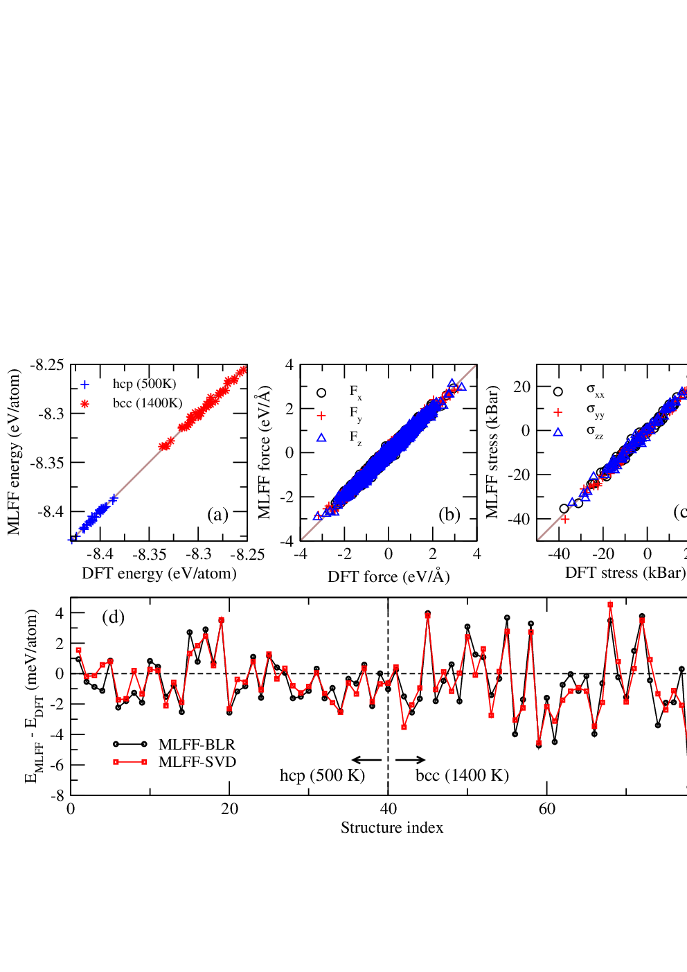
The generated MLFFs have been validated on a test dataset containing 40 hcp structures of 64 atoms at =500 K and another 40 bcc structures of 64 atoms at =1400 K. These structures were generated using MD simulations with an NPT ensemble at =500 and 1400 K employing the obtained MLFFs. Table 1 shows both the training and validation errors in energies, forces, and stress tensors calculated by MLFF-BLR and MLFF-SVD. Clearly, results using SVD are generally improved compared to the results using BLR, both for the test and training dataset. Although the improvement seems to be modest, we will see below that physical observables are also better described using the SVD. Concerning the relative weight of the energy equations, we note that using SVD the error in the energy in the training dataset decreases significantly, reaching sub meV precision (0.47 meV/atom), if the energy equations are reweighted by a factor of 100. Unfortunately, the errors in the test dataset increase, if is increased beyond a value of 10. This indicates that by strongly weighting the energy equations, the unregularized SVD tends to overfit the energies, and overall the best results on the test dataset are obtained by reweighting the energy equations by a factor of 10 and using SVD.
As an illustration, results on the energies, forces and diagonal components of stress tensors predicted by MLFF-SVD and density functional theory (DFT) for the test dataset are presented in Figs. 2(a)2(c), respectively, showing very good agreement. In addition, the MLFFs and DFT predicted energy difference for each structure in the test datasets is shown in Fig. 2(d). Compared to the hcp structures, the bcc ones exhibit larger errors due to the stronger thermal fluctuations at high temperature. We note that our generated MLFF-BLR is already very accurate with training and validation errors of 2.33 and 2.17 meV/atom in the energy, respectively. Due to the improved condition number, MLFF-SVD further improves upon MLFF-BLR by reducing the overall errors in energies, forces and stress tensors (see Table 1). These improvements are particularly relevant for the application to the prediction of defects energetics where supercells need to be used and errors in the range of 1 meV/atom will cause errors of the order of 100 meV for defects. In addition, as compared to MLFF-BLR, MLFF-SVD improves the phonon dispersions towards DFT results due to its improved forces, as will be discussed later on.
| DFT | BLR | SVD | Expt. | |
| hcp Zr | ||||
| (Å) | 3.235 | 3.234 | 3.235 | 3.233 Kolesnikov et al. 1994 |
| (Å) | 5.167 | 5.169 | 5.166 | 5.147 Kolesnikov et al. 1994 |
| bcc Zr | ||||
| (Å) | 3.574 | 3.574 | 3.573 | 3.551 Yasohama and Ogasawara 1974 |
| (bcc)(hcp) (eV/atom) | 0.084 | 0.081 | 0.082 | — |
We notice that our force field is more accurate than the one obtained by Zong et al. Zong et al. 2018, which exhibited much larger training mean absolute errors of 5.8 and 6.7 meV/atom in the energy for hcp and bcc Zr, respectively. This might be related to the fairly simplified ML model used in Ref. Zong et al. 2018 as well as a rather extensive training dataset containing multiphase structures. Surprisingly, the force field generated by Qian and Yang Qian and Yang 2018 shows rather small validation RMSE of 0.2 meV/atom for the hcp phase and 0.3 meV/atom for the bcc phase Qian and Yang 2018. In our experience, a precision of sub meV/atom can only be attained if fairly small displacements and low temperature structures are used. Indeed, the training structures considered in Ref. Qian and Yang 2018 correspond to small displacements of the groundstate hcp and bcc structure as well as finite temperature training data at 100, 300, and 1200 K, and validation was done for configurations selected from MD simulations at 300 K.
IV Results
We start by showing the lattice parameters of hcp and bcc Zr at 0 K as well as their energy difference predicted by DFT and MLFFs. As seen in Table 2, almost perfect agreement is observed between DFT and MLFFs for both BLR and SVD. The slightly larger lattice parameters predicted by theory as compared to experiment originate from the tendency of PBE to overestimate lattice constants. For the energy difference between bcc and hcp Zr, both MLFF-BLR and MLFF-SVD slightly underestimate the DFT value with MLFF-SVD being more accurate (see also Table 1).

Figure 3 presents the phonon dispersions of hcp and bcc Zr at 0 K calculated by DFT and MLFFs. Consistent with previous FP calculations Chen et al. 1985; Souvatzis et al. 2008; Zong et al. 2018; Qian and Yang 2018, at 0 K hcp Zr is dynamically stable, whereas bcc Zr is dynamically unstable due to the double-well shape of the potential energy surface Qian and Yang 2018. As compared to DFT, MLFF-BLR describes the acoustic phonons of hcp Zr very well. Although a slightly larger deviation exists for the optical phonons, it seems that difficulties in accurately describing optical phonons are quite general for machine learned interatomic potentials Zong et al. 2018; Qian and Yang 2018. For instance, our results are comparable with those predicted by Qian and Yang Qian and Yang 2018, but are better than those predicted by Zong et al. Zong et al. 2018. The latter show a very large discrepancy of nearly 2 THz for the optical phonons at the Brillouin-zone center Zong et al. 2018. The possible reasons have been discussed in Sec. III.3. Here, we want to emphasize that in contrast to Ref. Qian and Yang 2018 where the force field was purposely trained to model phonons by using perturbed supercells with strains and displacements, in the present work, the necessary information on the force constants were automatically captured during the on-the-fly MLFF training, and our MLFF predicted phonon dispersions came out to be in good agreement with the DFT results. In addition, we observe that the average optical phonon frequencies predicted by our MLFFs are quite accurate, which implies that free energy differences are likely to be described accurately. For the bcc phase, the MLFF-BLR is able to capture the soft zone-boundary -point phonon of the branch which is involved in the - phase transition Burgers 1934; Petry 1991 and the soft phonon mode in the - direction that is responsible for the - phase transition Stassis et al. 1978; Petry 1991; Sikka et al. 1982, but struggles to obtain accurate results along -. However, these soft phonon modes are extremely difficult to obtain accurately even by DFT, with the DFT results being strongly dependent on the system size. This means that training on a 48-atom cell is likely to be inadequate to describe all phonon instabilities in bcc Zr. As compared to MLFF-BLR, MLFF-SVD overall improves the phonon dispersions towards the DFT results for both hcp and bcc Zr, in particular for the optical phonon modes for both phases and the soft phonon modes along - for bcc Zr. This is not unexpected, since MLFF-SVD reduces errors in forces as compared to MLFF-BLR (see Table 1).

| DFT | BLR | SVD | SVD | Expt. | |
| (=1) | (=1) | (=5) | |||
| hcp Zr | |||||
| 143.4 | 133.9 | 132.0 | 140.7 | 155.4 | |
| (155.3) | (150.3) | (142.9) | (149.6) | – | |
| 64.9 | 78.0 | 61.8 | 63.2 | 67.2 | |
| (52.9) | (61.5) | (50.8) | (54.3) | – | |
| 65.4 | 68.6 | 56.7 | 62.8 | 64.6 | |
| 169.3 | 169.4 | 158.9 | 158.0 | 172.5 | |
| 24.4 | 26.7 | 24.5 | 24.0 | 36.3 | |
| 93.31 | 95.55 | 89.0 | 91.8 | 97.5 | |
| bcc Zr | |||||
| 73.3 | 109.0 | 72.3 | 76.7 | 104 | |
| 95.3 | 117.8 | 105.4 | 108.1 | 93 | |
| 28.8 | 39.5 | 36.5 | 32.7 | 38 | |
| 88.80 | 111.67 | 97.1 | 97.3 | — |
Another important quantity for the prediction of phase transition are the elastic properties, which are typically hard to accurately predict Zong et al. 2018; Qian and Yang 2018; Wimmer et al. 2020. Although our MLFFs were trained during a heating/cooling MD simulation at a constant zero pressure only (the focus of the present study is on the temperature-induced hcp-bcc phase transition at ambient pressure), it turns out that the fluctuations of the volumes in the MD simulation allow us to sample slightly strained structures and therefore our MLFFs are capable to describe elastic properties quite well. Indeed, Fig. 4 shows the volume dependence of the energies of hcp and bcc Zr at 0 K predicted by DFT and MLFFs. One observes that the DFT calculated energy vs. volume curve is well reproduced by our MLFFs. Obvious deviations are discernible only for small volumes away from the equilibrium volume. This is expected, because no external pressure is applied during training. The better agreement between DFT and MLFFs for the larger volumes apparently benefits from the thermal expansion during heating. As compared to the results in Ref. Zong et al. 2018, our MLFFs predicted energy vs. volume curves are, again, in better agreement with the DFT data. Table 3 summarizes the predicted elastic coefficients and bulk moduli. One can see that our MLFFs work well for the elastic properties of hcp Zr, showing reasonably good agreement with DFT. However, the description of the elastic properties for bcc Zr by our MLFFs is not so satisfactory. The largest discrepancy is found for . This is because at 0 K, the bcc phase is unstable both dynamically [see Fig. 3(b)] and mechanically [the Born elastic stability criterion () Born and Huang 1954 is disobeyed], and therefore, only few reference structures corresponding to the unstable ideal bcc phase are collected during our on-the-fly training. Concerning the comparison between MLFF-BLR and MLFF-SVD, we found that both MLFFs are comparably good in predicting the elastic properties of hcp Zr, whereas the MLFF-SVD dramatically improves over the MLFF-BLR for bcc Zr. In addition, by increasing by a factor of 5, the overall elastic properties are further improved, but this slightly worsens the phonon dispersion relations (see Fig. 3). This is expected, because increasing yields more accurate stress tensors, while slightly increasing the errors in energies and forces.

Finally, we turn to the hcp-bcc phase transition. To avoid large volume fluctuations appearing in small supercells, a reasonably large orthorhombic supercell with 180 Zr atoms is used to simulate the phase transition. Figure 5 shows the evolution of the volume with respect to the temperature during the heating and cooling MD simulations predicted by MLFF-BLR and MLFF-SVD. For each MD simulation, 2 million MD steps (corresponding to a heating/cooling rate 0.33 K/ps) were used. First, one can observe that both MLFFs successfully reproduce the hcp-bcc phase transition, a typical first-order phase transition manifested by an abrupt jump in the volume at . Second, the predicted phase transition between hcp and bcc phases is reversible via heating or cooling, but a fairly large hysteresis is observed, i.e., heating and cooling runs yield different . This is not unexpected for a first-order phase transition and similar to experimentally observed superheating and supercooling. Third, if we average over the upper and lower transition temperatures, both MLFFs predict a that is in reasonable agreement with the experimental value. However, as compared to the phonon dispersion relations, no improvement for the prediction of by SVD is obvious. We will explain this observation below.
We note that a quantitative comparison of between experiment and theory as obtained from direct heating and cooling should be done cautiously. For small systems, the transition temperatures might well be wrong by 100 K due to errors introduced by finite size effects or hysteresis. To mitigate this problem, we performed each heating or cooling run ten times to obtain a reasonable statistics for estimating , and we obtained a mean value of 1040 K with a standard deviation of 30 K for MLFF-SVD. Upon heating the lowest temperature at which the transition to the bcc structure occurred was 1107 K, while upon cooling the highest temperature at which the transition to the hcp structure occurred was 982 K. The mean (1045 K) is in excellent agreement with the above value. To refine the transition temperature further, we lowered the heating and cooling rate by a factor of 4 (0.08 K/ps) and performed four more cooling runs yielding transition temperatures of 1019-1047 K, as well as four more heating runs yielding transition temperatures of 1046-1093 K. These values clearly confirm that the transition temperature for a system size of 180 atoms is about 1045 K with an estimated error bar well below 10 K. Such a small error bar would be very hard to achieve using, for instance, thermodynamic integration and free energy methods.
Finally, we have explored how accurate the force fields, MLFF-BLR and MLFF-SVD, are compared to the reference PBE calculation. The previous assessments on the ideal hcp and bcc structures are not necessarily very accurate, since bcc Zr at 0 K is dynamically unstable, and finite temperature displacements are obviously not considered. To assess the accuracy of the MLFF for predictions of the transition temperature, we estimate the free energy difference between FP and MLFF calculations through thermodynamic perturbation theory (TPT) in the second-order cumulant expansion Zwanzig 1954; Dorner et al. 2018
| (16) |
where is the potential energy difference between FP and MLFF calculations. Without loss of generality, 40 structures close to =1040 K from the heating and cooling MD runs using MLFF-SVD were selected as test ensemble. The former (heating) are clearly hcp-like, whereas the later resemble bcc-like structures. The estimated values of are shown in Table 4. Obviously, MLFF-SVD is more accurate than MLFF-BLR for the free energies, in particular for the bcc Zr where a larger deviation of meV/atom from the FP free energy is observed in the MLFF-BLR. This is expected, since MLFF-SVD predicts more accurate potential energies as well as phonon dispersion relations. For the free energy difference between the bcc and hcp phases, which is relevant for estimating , MLFF-SVD and MLFF-BLR yield deviations of 0.27 and 0.84 meV/atom, respectively, as compared to the one calculated by PBE. After estimating the entropy difference between the two phases, we estimate that this translates to an error of 9 K for MLFF-SVD in predicting . With the correction by TPT, our final estimate for by PBE is placed at 1049 K, in reasonable agreement with the experimental value of 1136 K.
| Heating/ hcp | Cooling/ bcc | ||||
| BLR | SVD | BLR | SVD | ||
| 0.80 | 0.56 | 1.64 | 0.83 | ||


To further validate that the observed phase transition is from hcp to bcc, x-ray powder diffraction (XRD) patterns are simulated for snapshot structures picked from the MD trajectories. The results are shown in Fig. 6. From the XRD patterns, the hcp-bcc phase transition is unambiguously confirmed, in accordance with Fig. 5. Furthermore, the displacive nature of the phase transition can be visually observed from the changes in the atomic structure, as shown in Fig. 7. The cooperative movement of Zr atoms of alternating (011)β planes in the bcc phase along the opposite [01]β directions results in the hcp atomic stacking sequence, confirming the the Burgers mechanism for the temperature-driven bcc-hcp phase transition Burgers 1934.
Our good prediction for the hcp-bcc phase transition of Zr undoubtedly demonstrates the strength and accuracy of on-the-fly MLFF. In particular, almost no human interference was required during the training, which in the present study just involved heating and cooling of hcp and bcc Zr. In principle, the training can be done in less than a week, with the human effort of setting up the calculations being just few hours. As a matter of fact, testing the MLFF was a significantly more time-consuming endeavor in the present case. Our MLFF training strategies and analysis presented in this work can also be employed to study the temperature-dependent martensitic phase transitions in other materials such as other group-IV elements Ti and Hf and group-III elements Sc, Y, and La, with very little effort. In addition, the obtained force fields trained on hcp and bcc Zr at ambient pressure can be further trained by applying external pressure and by including the hexagonal phase in the training dataset so that the full temperature-pressure phase diagram of Zr can be readily constructed.
V Conclusions
To summarize, we have successfully applied the on-the-fly MLFF method to determine a force field for bcc and hcp Zr and study the hcp-bcc phase transition of Zr. This is a fairly challenging problem that is hard to address using brute force methods and FP MD simulations due to the limited length and time scales accessible to DFT simulations. Certainly, standard passive learning methods are possible and have been successfully used in the past, but they do not offer the same sort of convenience as the present approach. The first-order displacive nature of the hcp-bcc phase transition— manifested by an abrupt jump in the system volume and a change in the atomic stacking sequences —has been unambiguously reproduced by our MD simulations and identified by the simulated XRD patterns, confirming the Burgers mechanism for the temperature-induced hcp-bcc phase transition. In addition, our MLFF predicted phase transition temperature is found to be in reasonable agreement with experiment. Finally, we have shown that due to the improved condition number, SVD is in general more accurate than the regularized BLR, which is evidenced by the systematic decrease of the errors in energies, forces, and stress tensors for both the training and test datasets. The improvement by SVD over BLR has also been showcased by its improved prediction of the energy difference between bcc and hcp Zr and of the phonon dispersions of both hcp and bcc Zr. In summary, evidence shown in this paper suggests that pseudo inversion of the design matrix using SVD is a useful approach to overcome some of the limitations of regularized regression methods.
Acknowledgements.
We thank E. Wimmer and J. Wormald for helpful discussions about this work. This work was funded by the Advanced Materials Simulation Engineering Tool (AMSET) project, sponsored by the US Naval Nuclear Laboratory (NNL) and directed by Materials Design, Inc.References
- Northwood (1985) D. O. Northwood, Materials & Design 6, 58 (1985).
- Kalavathi and Kumar Bhuyan (2019) V. Kalavathi and R. Kumar Bhuyan, Materials Today: Proceedings 19, 781 (2019).
- Vogel and Tonn (1931) R. Vogel and W. Tonn, Z. Anorg. Allgem. Chem. 202, 292 (1931).
- Fisher and Renken (1964) E. S. Fisher and C. J. Renken, Phys. Rev. 135, A482 (1964).
- Olinger and Jamieson (1973) B. Olinger and J. C. Jamieson, High. Temp.-High. Press. 5, 123 (1973).
- Sikka et al. (1982) S. Sikka, Y. Vohra, and R. Chidambaram, Progress in Materials Science 27, 245 (1982).
- Xia et al. (1990) H. Xia, S. J. Duclos, A. L. Ruoff, and Y. K. Vohra, Phys. Rev. Lett. 64, 204 (1990).
- Xia et al. (1991) H. Xia, A. L. Ruoff, and Y. K. Vohra, Phys. Rev. B 44, 10374 (1991).
- Song and III (1995) S. G. Song and G. T. G. III, Philosophical Magazine A 71, 275 (1995).
- Zhao et al. (2005) Y. Zhao, J. Zhang, C. Pantea, J. Qian, L. L. Daemen, P. A. Rigg, R. S. Hixson, G. T. Gray, Y. Yang, L. Wang, Y. Wang, and T. Uchida, Phys. Rev. B 71, 184119 (2005).
- Zhang et al. (2005) J. Zhang, Y. Zhao, C. Pantea, J. Qian, L. L. Daemen, P. A. Rigg, R. S. Hixson, C. W. Greeff, G. T. Gray, Y. Yang, L. Wang, Y. Wang, and T. Uchida, Journal of Physics and Chemistry of Solids 66, 1213 (2005).
- Liu et al. (2008) W. Liu, B. Li, L. Wang, J. Zhang, and Y. Zhao, Journal of Applied Physics 104, 076102 (2008).
- Akahama et al. (1991) Y. Akahama, M. Kobayashi, and H. Kawamura, Journal of the Physical Society of Japan 60, 3211 (1991).
- Akahama et al. (1992) Y. Akahama, M. Kobayashi, and H. Kawamura, High Pressure Research 10, 711 (1992).
- Ostanin and Trubitsin (1998) S. A. Ostanin and V. Y. Trubitsin, Phys. Rev. B 57, 13485 (1998).
- Stavrou et al. (2018) E. Stavrou, L. H. Yang, P. Söderlind, D. Aberg, H. B. Radousky, M. R. Armstrong, J. L. Belof, M. Kunz, E. Greenberg, V. B. Prakapenka, and D. A. Young, Phys. Rev. B 98, 220101 (2018).
- Burgers (1934) W. Burgers, Physica 1, 561 (1934).
- Petry (1991) W. Petry, Phase Transitions 31, 119 (1991).
- Ahuja et al. (1993) R. Ahuja, J. M. Wills, B. Johansson, and O. Eriksson, Phys. Rev. B 48, 16269 (1993).
- Greeff (2005) C. W. Greeff, Modelling and Simulation in Materials Science and Engineering 13, 1015 (2005).
- Schnell and Albers (2006) I. Schnell and R. C. Albers, Journal of Physics: Condensed Matter 18, 1483 (2006).
- Souvatzis et al. (2011) P. Souvatzis, S. Arapan, O. Eriksson, and M. I. Katsnelson, EPL (Europhysics Letters) 96, 66006 (2011).
- Chen et al. (1985) Y. Chen, C.-L. Fu, K.-M. Ho, and B. N. Harmon, Phys. Rev. B 31, 6775 (1985).
- Zong et al. (2018) H. Zong, G. Pilania, X. Ding, G. J. Ackland, and T. Lookman, npj Computational Materials 4, 48 (2018).
- Souvatzis et al. (2008) P. Souvatzis, O. Eriksson, M. I. Katsnelson, and S. P. Rudin, Phys. Rev. Lett. 100, 095901 (2008).
- Qian and Yang (2018) X. Qian and R. Yang, Phys. Rev. B 98, 224108 (2018).
- Stassis et al. (1978) C. Stassis, J. Zarestky, and N. Wakabayashi, Phys. Rev. Lett. 41, 1726 (1978).
- Ye et al. (1987) Y. Y. Ye, Y. Chen, K. M. Ho, B. N. Harmon, and P. A. Lindgrd, Phys. Rev. Lett. 58, 1769 (1987).
- Heiming et al. (1991) A. Heiming, W. Petry, J. Trampenau, M. Alba, C. Herzig, H. R. Schober, and G. Vogl, Phys. Rev. B 43, 10948 (1991).
- Hu et al. (2011) C.-E. Hu, Z.-Y. Zeng, L. Zhang, X.-R. Chen, and L.-C. Cai, Computational Materials Science 50, 835 (2011).
- Willaime and Massobrio (1989) F. m. c. Willaime and C. Massobrio, Phys. Rev. Lett. 63, 2244 (1989).
- Zong et al. (2020) H. Zong, P. He, X. Ding, and G. J. Ackland, Phys. Rev. B 101, 144105 (2020).
- Hellman et al. (2011) O. Hellman, I. A. Abrikosov, and S. I. Simak, Phys. Rev. B 84, 180301 (2011).
- Willaime and Massobrio (1991) F. Willaime and C. Massobrio, Phys. Rev. B 43, 11653 (1991).
- Mendelev and Ackland (2007) M. I. Mendelev and G. J. Ackland, Philosophical Magazine Letters 87, 349 (2007).
- Behler and Parrinello (2007) J. Behler and M. Parrinello, Phys. Rev. Lett. 98, 146401 (2007).
- Bartók et al. (2010) A. P. Bartók, M. C. Payne, R. Kondor, and G. Csányi, Phys. Rev. Lett. 104, 136403 (2010).
- Behler (2017) J. Behler, Angewandte Chemie International Edition 56, 12828 (2017).
- Botu et al. (2017) V. Botu, R. Batra, J. Chapman, and R. Ramprasad, The Journal of Physical Chemistry C 121, 511 (2017).
- De et al. (2016) S. De, A. P. Bartók, G. Csányi, and M. Ceriotti, Phys. Chem. Chem. Phys. 18, 13754 (2016).
- Schmidt et al. (2019) J. Schmidt, M. R. G. Marques, S. Botti, and M. A. L. Marques, npj Computational Materials 5, 83 (2019).
- Bartók et al. (2013) A. P. Bartók, R. Kondor, and G. Csányi, Phys. Rev. B 87, 184115 (2013).
- Li et al. (2015) Z. Li, J. R. Kermode, and A. De Vita, Phys. Rev. Lett. 114, 096405 (2015).
- Jacobsen et al. (2018) T. L. Jacobsen, M. S. Jørgensen, and B. Hammer, Phys. Rev. Lett. 120, 026102 (2018).
- Jinnouchi et al. (2019a) R. Jinnouchi, J. Lahnsteiner, F. Karsai, G. Kresse, and M. Bokdam, Phys. Rev. Lett. 122, 225701 (2019a).
- Jinnouchi et al. (2019b) R. Jinnouchi, F. Karsai, and G. Kresse, Phys. Rev. B 100, 014105 (2019b).
- Jinnouchi et al. (2020a) R. Jinnouchi, F. Karsai, and G. Kresse, Phys. Rev. B 101, 060201 (2020a).
- Jinnouchi et al. (2020b) R. Jinnouchi, K. Miwa, F. Karsai, G. Kresse, and R. Asahi, The Journal of Physical Chemistry Letters 11, 6946 (2020b).
- Seko et al. (2014) A. Seko, A. Takahashi, and I. Tanaka, Phys. Rev. B 90, 024101 (2014).
- Shapeev (2016) A. V. Shapeev, Multiscale Modeling & Simulation 14, 1153 (2016).
- Glielmo et al. (2018) A. Glielmo, C. Zeni, and A. De Vita, Phys. Rev. B 97, 184307 (2018).
- Faber et al. (2018) F. A. Faber, A. S. Christensen, B. Huang, and O. A. von Lilienfeld, The Journal of Chemical Physics 148, 241717 (2018).
- Jinnouchi et al. (2020c) R. Jinnouchi, F. Karsai, C. Verdi, R. Asahi, and G. Kresse, The Journal of Chemical Physics 152, 234102 (2020c).
- Bishop (2006) C. M. Bishop, Pattern Recognition and Machine Learning (Information Science and Statistics) (Springer, New York, 2006).
- Szlachta et al. (2014) W. J. Szlachta, A. P. Bartók, and G. Csányi, Phys. Rev. B 90, 104108 (2014).
- Blackford et al. (1997) L. S. Blackford, J. Choi, A. Cleary, E. D’Azevedo, J. Demmel, I. Dhillon, J. Dongarra, S. Hammarling, G. Henry, A. Petitet, K. Stanley, D. Walker, and R. C. Whaley, ScaLAPACK Users’ Guide (Society for Industrial and Applied Mathematics, Philadelphia, PA, 1997).
- Tikhonov et al. (1995) A. N. Tikhonov, A. Goncharsky, V. V. Stepanov, and A. G. Yagola, Numerical Methods for the Solution of Ill-Posed Problems (Springer, New York, 1995).
- Kresse and Hafner (1993) G. Kresse and J. Hafner, Phys. Rev. B 47, 558 (1993).
- Kresse and Furthmüller (1996) G. Kresse and J. Furthmüller, Phys. Rev. B 54, 11169 (1996).
- Perdew et al. (1996) J. P. Perdew, K. Burke, and M. Ernzerhof, Phys. Rev. Lett. 77, 3865 (1996).
- (61) M. P. Allen and D. J. Tildesley, Computer simulation of liquids (Oxford university press: New York, 1991).
- Kolesnikov et al. (1994) A. I. Kolesnikov, A. M. Balagurov, I. O. Bashkin, A. V. Belushkin, E. G. Ponyatovsky, and M. Prager, Journal of Physics: Condensed Matter 6, 8977 (1994).
- Yasohama and Ogasawara (1974) K. Yasohama and T. Ogasawara, Journal of the Physical Society of Japan 36, 1349 (1974).
- Vinet et al. (1989) P. Vinet, J. H. Rose, J. Ferrante, and J. R. Smith, Journal of Physics: Condensed Matter 1, 1941 (1989).
- Wimmer et al. (2020) E. Wimmer, M. Christensen, W. Wolf, W. Howland, B. Kammenzind, and R. Smith, Journal of Nuclear Materials 532, 152055 (2020).
- Born and Huang (1954) M. Born and K. Huang, Dynamical Theory of Crystal Lattices (Clarendon, Oxford, 1954).
- Zwanzig (1954) R. W. Zwanzig, The Journal of Chemical Physics 22, 1420 (1954).
- Dorner et al. (2018) F. Dorner, Z. Sukurma, C. Dellago, and G. Kresse, Phys. Rev. Lett. 121, 195701 (2018).