Ratio of counts vs ratio of rates
in Poisson processes

The probability density function of $\lambda$ is evaluated from the so called Bayes’ rule:

where $f_{0}(\lambda)$ is the so called ‘prior’.⁹⁹ 9 This name is somehow unfortunate, because it might induce people think to time order, as discussed in Ref. [1], in which it is shown how, instead, the ‘prior’ can be applied in a second step, in particular by someone else, if a ‘flat prior’ used. Assuming for the moment a ‘flat’ prior, that is $f_{0}(\lambda)=k$, and neglecting all factors non depending on $\lambda$, we get

in which we recognize a Gamma pdf with $\alpha=x+1$ and $\beta=1$ (see Appendix A – for a detailed derivation see e.g. Ref. [13]), and therefore

Expected value, standard deviation and mode are $x+1$, $\sqrt{x+1}$ and $x$, respectively. The advantage of having expressed the distribution of $\lambda$ in terms of a Gamma is that we can use the probability distributions made available from programming languages, e.g. in R, which usually include also useful random generators (e.g. rgamma() in R). For example, making use of the R function dgamma() we can draw Fig. 4,

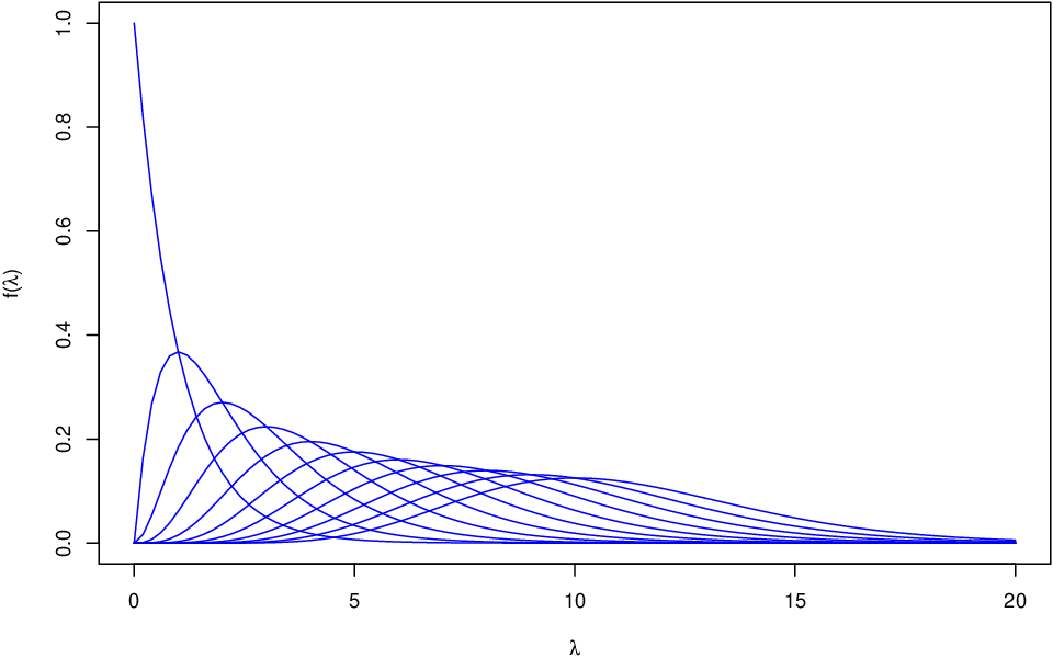
which shows $f(\lambda\,|\,x)$, for $x=1,2,\ldots,10$, with the following few lines of code:

for (x.o in 0:10) {
  curve(dgamma(x,x.o+1,1),xlim=c(0,20),ylim=c(0,1),col=’blue’,add=x.o>0,
        xlab=expression(lambda),ylab=expression(paste(’f(’,lambda,’)’)))
}

Once we have learned that the pdf of $\lambda$, in the light of the observation of $x$ count and assuming a flat prior, is a Gamma distribution, the easiest way to evaluate the distribution of $\lambda_{1}/\lambda_{2}$, for $x_{2}>0$, is by sampling. For example, using the following lines of R code,

x1 = 1
x2 = 1
lambda1 = rgamma(n, x1+1, 1)
lambda2 = rgamma(n, x2+1, 1)
rho = lambda1/lambda2

Then, varying x1 and x2 we can get the plots of Figs. 5 and 6.¹⁰¹⁰ 10 The complete script is provided in Appendix B.2.

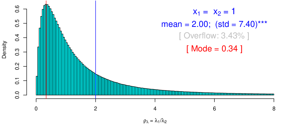
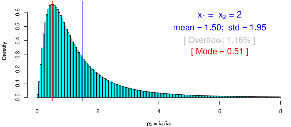
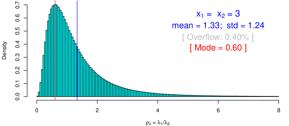
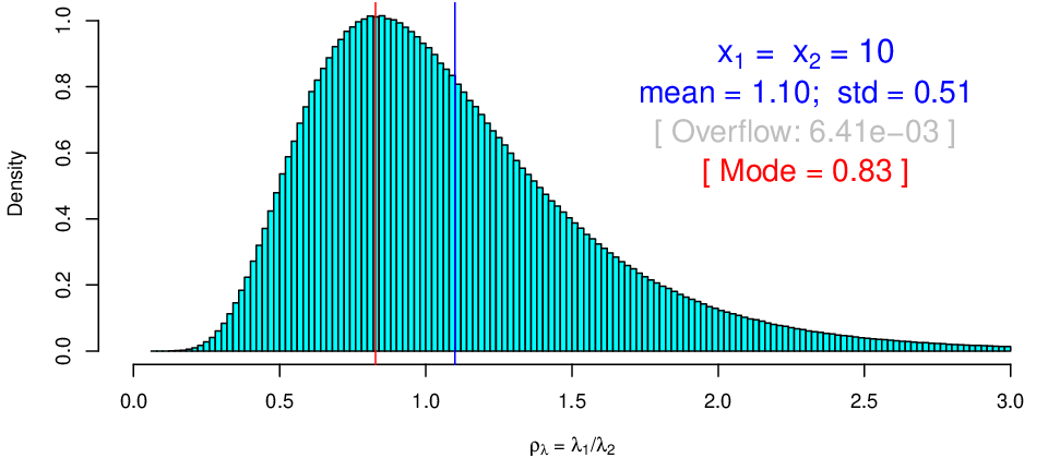
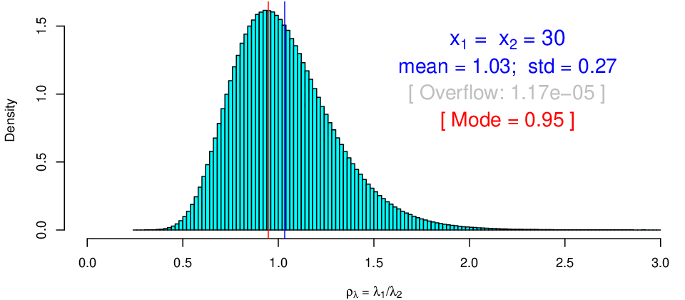
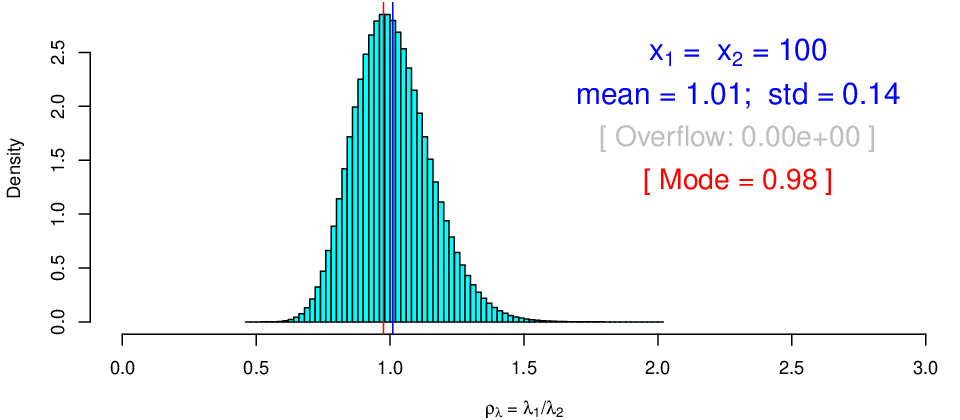
We immediately observe that the histograms are very regular, without divergences, although for small values of $x_{2}$ there is quite a long tail up to infinity, which is however reached with vanishing probability (the figures report also the proportions of overflows, having chosen the horizontal scale of the plots in order to show the most interesting part of each probability distribution). The mean and standard deviation (‘std’) shown on each plot are calculated from the Monte Carlo samples.

The effect of the long tails is that there is quite a big difference between mean value and the most probable one, located around the highest bar of the histogram. This is not a surprise (the famous exponential distribution has modal value equal to zero independently of its parameter!), but it should sound as a warning for those who use analysis methods which provide, as ‘estimator’, ‘‘the most probable value’’¹¹¹¹ 11 For the reason of the quote marks see footnote 8. [13]. Moreover, for very small $x_{2}$ the tails do not seem to go very fast to zero (in comparison e.g. to the exponential), leading to not-defined moments of the distribution (of the theoretical one, obviously, since in most cases mean and standard deviation of the Monte Carlo distribution have finite values). This question will be investigated in the next subsection, after the derivation of closed expressions.

When $x_{1}$ and $x_{2}$ become ‘quite large’ the Gamma distribution tends (slowly – think to the $\chi^{2}$, that is indeed a particular Gamma, as reminded in Appendix A) to a Gaussian, and likewise does (a bit slower) the ratio of two Gamma variables (as $\lambda_{1}$ and $\lambda_{2}$ are), as we can see for the case $x_{1}\!=\!x_{2}\!=\!100$ of Fig. 6,¹²¹² 12 Zero overflow in that plot is only due to the ‘limited’ number of sampled, chosen to be $10^{7}$, and to the fact that the same script of the other plot has been used. in which some skewness is still visible and the mode is about $3\%$ smaller than the mean value.

Being the evaluation of ratio of rates (to which the ratio of $\lambda$’s is related) an important issue in Physics, it is worth trying to get an analytic expression for its pdf. This can be done extending to the continuum Eq. (2),¹³¹³ 13 for a different approach to get Eq. (13) see footnote 13 , in which the integrand of Eq. (13) is interpreted as the joint pdf of $\rho_{\lambda}$, $\lambda_{1}$ and $\lambda_{2}$. that is replacing the sums by integrals, and applying the constraint between the two variables by a Dirac delta [13]:

Making use of the properties of the $\delta()$, we can rewrite it as

with $\lambda_{1}^{*}$ root of the equation $\rho_{\lambda}-\lambda_{1}/\lambda_{2}=0$, and therefore equal to $\rho_{\lambda}\cdot\lambda_{2}$. Equation (13) becomes then

Once more we recognize in the integrand something related to the Gamma distribution. In fact, identifying the power of $\lambda_{2}$ with ‘$\alpha-1$’ of a Gamma pdf, and ‘$(1+\rho_{\lambda})$’ at the exponent with the ‘rate parameter’ $\beta$, that is

the integrand in Eq. (18) can be rewritten as

in order to recognize within parentheses a Gamma pdf in the variable $\lambda_{2}$, whose integral over $\lambda_{2}$ is then equal to one because of normalization. We get then

The mode of the distribution can be easily obtained finding the maximum (of the log) of the pdf, thus getting

in agreement with what we have got in Figs. 5 and 6 by Monte Carlo (indeed, done there in a fast and rather rough way – see Appendix B.2).

In order to get expected value and standard deviation, we need to evaluate the relevant integrals¹⁴¹⁴ 14 Work done on a Raspberry Pi3, thanks to Mathematica 12.0 generously offered by Wolfram Inc. to the Raspbian system.

• •

  First we check that $f(\rho_{\lambda}\,|\,x_{1},x_{2})$ is properly normalized. Indeed the integral $\int_{0}^{\infty}\!f(\rho_{\lambda}\,|\,x_{1},x_{2})\,\mbox{d}\rho_{\lambda}$ is equal to unity for ‘all possible’ $x_{1}$ and $x_{2}$.¹⁵¹⁵ 15 To be precise, the condition is $x_{1}>-1$ and $x_{2}>-1$, but, given the role of the two variables in our context, it means for all possible counts (including $x_{1}=x_{2}=0$, for which the pdf becomes $1/(1+\rho_{\lambda})^{2}$, having however infinite mean and variance.)

• •

  The expected value is equal to

  $\displaystyle\mbox{E}(\rho_{\lambda}\,|\,x_{1},x_{2})$

  $\displaystyle=$

  $\displaystyle\frac{x_{1}+1}{x_{2}}\hskip 19.91684pt(\mathbf{x_{2}>0})\,,$

  (27)

  in perfect agreement with what we can read from the Monte Carlo results of Figs. 5 and 6.

• •

  The expected value of $\rho_{\lambda}^{2}$ is given by

  $\displaystyle\mbox{E}(\rho_{\lambda}^{2}\,|\,x_{1},x_{2})$

  $\displaystyle=$

  $\displaystyle\frac{(x_{1}+1)\cdot(x_{1}+2)}{x_{2}\cdot(x_{2}-1)}\hskip 85.35826pt(\mathbf{x_{2}>1})\,,$

  (28)

  from which we evaluate (subtracting to it the square of the expected value)

  $\displaystyle\mbox{Var}(\rho_{\lambda}\,|\,x_{1},x_{2})$

  $\displaystyle=$

  $\displaystyle\frac{x_{1}+1}{x_{2}}\cdot\left(\frac{x_{1}+2}{x_{2}-1}-\frac{x_{1}+1}{x_{2}}\right)\hskip 22.76228pt(\mathbf{x_{2}>1})\,,$

  (29)

  from which the standard deviation follows, that we rewrite in a more compact form as

  $\displaystyle\sigma(\rho_{\lambda})$

  $\displaystyle=$

  $\displaystyle\sqrt{\mu_{\rho_{\lambda}}\cdot\left(\frac{x_{1}+2}{x_{2}-1}-\mu_{\rho_{\lambda}}\right)}\hskip 113.81102pt(\mathbf{x_{2}>1})\,,$

  (30)

  having indicated by $\mu_{\rho_{\lambda}}$ the expected value of $\rho_{\lambda}$. For the values $x_{1}$ and $x_{2}$ used in Figs. 5 and 6, we get, starting from $\mathbf{x_{1}=x_{2}=2}$ in increasing order, the following standard deviations: 1.936, 1.247, 0.507, 0.269 and 0.143, in agreement with the Monte Carlo results (or the other way around).

The detailed comparison between closed expression of the pdf and the Monte Carlo outcome is shown in Fig. 7 for the toughest case we have met, that is $x_{1}=x_{2}=1$.

Being $r$ equal to $\lambda/T$, we can obtain its pdf by a simple change of variables.¹⁸¹⁸ 18 Starting from $f(\lambda\,|\,x)$ given by Eq. (12) we get $\displaystyle f(\lambda\,|\,x)\,\mbox{d}\lambda\,=\,\frac{\lambda^{x}\cdot e^{-\lambda}}{x!}\,\mbox{d}\lambda$ $\displaystyle=$ $\displaystyle\frac{(r\cdot T)^{x}\cdot e^{-r\,T}}{x!}\cdot T\,\mbox{d}r\,=\,f(r\,|\,x,T)\,\mbox{d}r$ $\displaystyle f(r\,|\,x,T)$ $\displaystyle=$ $\displaystyle\frac{T^{x+1}\cdot r^{x}\cdot e^{-T\,r}}{x!}\,.$ in which we recognize a Gamma pdf with $\alpha=x+1$ and $\beta=T$. But, having practiced a bit with the Gamma distribution, we can reach the identical result observing that, using again a flat prior and neglecting irrelevant factors, the pdf of $r$ is given by

in which we recognize, besides the normalization factor, a Gamma pdf for the variable $r$ with $\alpha=x+1$ and $\beta=T$, and hence

Mode, expected value and standard deviation of $r$ are then (see Appendix A)

as also expected from the ‘summaries’ of $f(\lambda\,|\,x)$ and making use of $r=\lambda/T$.
$[$ Note that the pdf (36) assumes, as explicitly written in the condition, a precise value of $T$. If this is not the case and $T$ is uncertain, then, similarly to what we have seen in footnote 3, the pdf of $r$ is evaluated as $f(r\,|\,x,I)=\int_{0}^{\infty}f(r\,|\,x,T,I)\cdot f(T\,|\,I)\,\mbox{d}T$. $]$

The very essence of the so called probabilistic inference (‘Bayesian inference’) is given by Eq. (31). The rest is just a question of normalization and of extending it to the continuum, that in our case of interest is

It is evident the symmetric role of $f(x\,|\,r,T,I)$ and $f(r\,|\,I)$, if the former is seen as a mathematical function of $r$ for a given (‘observed’) $x$, that is $x$ playing the role of a parameter. This function is known as likelihood and commonly indicated by ${\cal L}(r\,;\,x,T)$.¹⁹¹⁹ 19 The real issue with the ‘likelihood’ is not just replacing in Eq. (37) $f(x\,|\,r,T,I)$ by ${\cal L}(r\,;\,x,T)$, but rather the fact, that, being this a function of $r$, it is perceived as ‘the likelihood of $r$’. The result is that it is often (almost always) turned by practitioners into ‘probability of $r$’, being ‘likelihood’ and ’probability’ used practically as synonyms in the spoken language. It follows, for example, that the value that maximizes the likelihood function is perceived as the ‘most probable’ value, in the light of the observations. Indicating the second factor of Eq. (37), that is the ‘infamous’ prior that causes so much anxiety in practitioners [8], by $f_{0}(r)$, we get (assuming $I$ implicit, as it is usually the case)

which makes it clear that we have two mathematical functions of $r$ playing symmetric and peer roles. Stated in different words, each of the two has the role of ‘reshaping’ the other [1]. In usual ‘routine’ measurements (as watching your weight on a balance) the information provided by ${\cal L}(\ldots)$ is so much narrower, with respect to $f_{0}(\ldots)$,²⁰²⁰ 20 This is true unless the balance shows a ‘clear anomaly’, and then you stick to what you believed your weight should be. But you still learn something from the measurement, indeed: the balance is broken [13]. that we can neglect the latter and absorb it in the proportionality factor, as we have done above in Sec. 3.1. Employing a uniform ‘prior’ is then usually a good idea to start with, unless $f_{0}(\ldots)$ arises from previous measurements or from strong theoretical prejudice on the quantity of interest. It is also very important to understand that ‘the reshaping’ due to the priors can be done in a second step, as it has been pointed out, with practical examples, in Ref. [1].

Let us now see what happens when, in our case, the Bayes rule is applied in sequence in order to account for several results on the same rate $r$, that is assumed to be stable. Imagine we start from rather vague ideas about the value of $r$, such that $f_{0}(r)=k$ is, in practice, the best practical choice we can do. After the observation of $x_{1}$ counts during $T_{1}$ we get, as we have learned above,

Then we perform a new campaign of observations and record $x_{2}$ counts in $T_{2}$. It is clear now that in the second inference we have to use as ‘prior’ the piece of knowledge derived from the first inference. So, we have, all together, besides irrelevant factors,

that is exactly as we had done a single experiment, observing $x_{tot}=x_{1}+x_{2}$ counts in $T_{tot}=T_{1}+T_{2}$. The only real physical strong assumption is that the intensity of Poisson process was the same during the two measurements, i.e. we have being measuring the same thing.

This teaches us immediately how to ‘combine the results’, an often debated subject within experimental teams, if we have sets of counts $x_{i}$ during times $T_{i}$ (indicated all together by ’$\underline{x}$’ and ‘$\underline{T}$’):

without imaginative averages or fits. But this does not mean that we can blindly sum up counts and measuring times. Needless to say, it is important, whenever it is possible, to make a detailed study of the behavior of $f(r\,|\,x_{i}\,T_{i})$ in order to be sure that the intensity $r$ is compatible with being constant during the measurements. But, once we are confident about its constancy (or that there is no strong evidence against that hypothesis), the result is provided by Eq. (43), from which all summaries of interest can be derived.²¹²¹ 21 It is perhaps important to remind that in probability theory the full result of the inference is the probability distribution (typically a pdf, for continuous quantities) of the quantity of interest as inferred from the data, the model and all other pertinent pieces of information. Mode, mean, median, standard deviation and probability intervals are just useful numbers to summarize with few numbers the distribution, with should always be reported, unless it is (with some degree of approximation) as simple as a Gaussian, so that mean and standard deviation provide the complete information. For example, the shape of a not trivial pdf can be expressed with coefficients of a suitable fit made in the region of interest. Or one can provide several moments of a distribution, from which the pdf can be reobtained (see e.g. Ref. [22]).

Let us consider again Eq. (38) and focus on the role of the likelihood to reshape $f_{0}(r)$. Being multiplicative factor irrelevant, it can be useful to rewrite that equation as

with $r_{R}$ a reference value, in principle arbitrary, but conceptually very interesting if properly chosen. In fact, the ratio in the above formula acquires the meaning of relative belief update factor [13, 17, 23],²²²² 22 Note how at that time we wrote Eq. (44) in a more expanded way, but the essence of this factor is given by Eq. (45). For recent developments and applications see Refs. [24, 25, 26]. and the updating Bayes’ rule can be rewritten as

This way of rewriting the Bayes’ rule is particularly convenient when the likelihood is not ’closed’, that is it does not go to zero when the quantity of interest is ‘very large’ or ‘very small’.

To be clear, let us make the example of having observed zero counts, that is the experiment was indeed performed, but no event of interest was found during the measurement time $T$. If we use a flat prior and only stick to the summaries, we have that the most probable value is zero, with $\mbox{E}(r)=\sigma(r)=1/T$: the larger is the measuring time, the more the distribution of $r$ is squeezed towards zero. But this does not give a complete picture of what is going on. Since ${\cal L}(r;x=0,T)$ goes to 1 for $r\rightarrow 0$, the likelihood is opened in the left side. Figure 9 shows ${\cal R}$

functions for this case, for different $T$, although in this very simple case ${\cal R}$ is mathematically equivalent to the likelihood.²³²³ 23 The more interesting case, originally taken into account in Refs. [17, 23], is when some events are observed, which could be, however, also attributed to irreducible background. If our beliefs about $r$ were above O($100\,\mbox{s}^{-1}$), the observation of zero events practically rule them out, even with $T=1\,$s (‘1 s’ is arbitrarily chosen in this hypothetical example, just to remind that both $T$ and $r$ have physical dimensions).

If we run the experiment longer and longer, keeping observing zero events, the possible values of $r$ gets smaller and smaller. What is mostly interesting, in this plot, is the region in which ${\cal R}$ is flat: it means that if our beliefs are concentrate there, then the experiment does not teach us more than what we already believed: the experiment looses sensitivity in that region and then reporting ‘probabilistic’ upper limits makes no sense and it can be highly misleading (even more reporting ‘C.L. upper limits‘) [13, 27].

At this point a technical remark is in order. The reason why the Gamma appears so often is that the expression of the Poisson probability function, seen as a function of $\lambda$ and neglecting multiplicative factors, that is $f(\lambda)\propto\lambda^{x}\cdot\exp(-\lambda)$, has the same structure of a Gamma pdf. The same is true if the variable $r$ is considered, that is $f(r)\propto r^{x}\cdot\exp(-T\cdot r)$. If then we have a Gamma distribution as prior, with parameters $\alpha_{0}$ and $\beta_{0}$, the ‘final’ distributions is still a Gamma:

This kind of distributions, such that the ‘posterior’ belongs to the same family of the ‘prior’, with updated parameters, are called conjugate priors for obvious reasons, as it is rather obvious how convenient they are in applications, provided they are flexible enough to describe ‘somehow’ the prior belief.²⁴²⁴ 24 Remember that, as Laplace used to say, “the theory of probabilities is basically just common sense reduced to calculus”, that “All models are wrong, but some are useful” (G.Cox) and that even Gauss was ‘sorry’ because ‘his’ error function could not be strictly true [28] (see quote in footnote 9 of Ref. [29]). This was particularly important at the times when the monstrous computational power nowadays available was not even imaginable (also the development of logical and mathematical tools has a strong relevance). Therefore a quite rich collection of conjugate priors is available in the literature (see e.g. Ref. [30]).

In sum, these are the updating rules of the Gamma parameters for our cases of interest (the subscript ’$f$’ is to remind that is the parameter of the ‘final’ distribution):

(Note that in the case of $r$ the parameter $\beta$ has the dimension of a time, being $r$ a rate, that is counts per unit of time.) A flat prior distribution is recovered for $\alpha_{0}=1$ and $\beta_{0}\rightarrow 0$. Technically, for $\alpha=1$ a Gamma distribution turns into a negative exponential: if then the ‘rate parameter’ $\beta$ is chosen to be very small, the exponential becomes ‘essentially flat’ in the region of interest.

Once we have learned the updating rules (50)-(51) and (52)-(53), it might be convenient to turn a prior expressed in terms of mean $\mu_{0}$ and standard deviation $\sigma_{0}$ into $\alpha_{0}$ and $\beta_{0}$, inverting the expressions of expected value and standard deviation of a Gamma distributed variable (see Appendix A), thus getting

For example, if we have good reason to think that $r$ should be $(5\pm 2)\,\mbox{s}^{-1}$​, the parameters of our initial Gamma distribution are $\alpha_{0}=6.25$ and $\beta_{0}=1.25\,\mbox{s}$. This is equivalent to having started from a flat prior and having observed (rounding the numbers) 5 counts in about 1.2 seconds. This gives a clear idea of the ‘strength’ of the prior – not much in this case, but it certainly excludes the possibility of $r=0$. This happens in fact as soon as $\alpha_{0}$ is larger then 1, implying $r^{\alpha_{0}-1}$ vanishing at $r=0$. This observation can be a used as a trick to forbid a vanishing value of $\lambda$ or of $r$, if we have good physical reason to believe that they cannot be zero, although we are highly uncertain about even their order of magnitude: just choose a prior $\alpha_{0}$ slightly larger than one.

References

- [1] G. D’Agostini and A. Esposito, Checking individuals and sampling populations with imperfect tests, arXiv:2009.04843 [q-bio.PE].
- [2] W. Nelson, Confidence intervals for the ratio of two Poisson means and Poisson predictor intervals, IEEE Trans. on Reliability, Vol. R-19 (1970) 42-49.
- [3] F. James and M Roos, Errors on ratios of small numbers of events, Nuclear Physics B172 (1980) 475-470.
- [4] K.J. Coakley, D.S. Simons and A.M. Leifer, Secondary ion mass spectroscopy measurements in isotopic ratios: corrections for time varying count rate, Int. J. of Mass Spectrometry 240 (2005) 107-120.
- [5] K. Gu, H.K.T. Ng, M.L. Tang and W.R. Schucany, Testing the ratio of two Poisson rates, Biometrical Journal 50 (2008) 283-298.
- [6] R.C. Ogliore, G.R. Huss and K. Nagashima, Ratio estimation in SIMS analysis, Nucl. Instr. and Meth, in Phys. Reas. B269 (2011) 1910-1918.
- [7] C.D. Coath, R.C.J. Steele and W.F. Lunnon, Statistical bias in isotope ratios, J. Anal. At. Spectrom., 2013, 28, 52-58.
- [8] G. D’Agostini, Overcoming priors anxiety, Bayesian Methods in the Sciences, J. M. Bernardo Ed., special issue of Rev. Acad. Cien. Madrid, Vol. 93, Num. 3, 1999, arXiv:physics/9906048 [physics.data-an].
- [9] International Organization for Standardization (ISO), Guide to the expression of uncertainty in measurement, Geneva, Switzerland, 1993.
- [10] https://en.wikipedia.org/wiki/Skellam_distribution .
- [11]
R Core Team (2018), R: A language and environment for statistical
computing. R Foundation for Statistical Computing, Vienna, Austria.
https://www.R-project.org/ . - [12]
J.W. Lewis et al., Package ‘skellam’,
https://CRAN.R-project.org/package=skellam . - [13] G. D’Agostini, Bayesian Reasoning in Data Analysis. A critical Introduction, World Scientific, 2003.
- [14] G. D’Agostini, Bayesian reasoning versus conventional statistics in High Energy Physics, Proc. XVIII International Workshop on Maximum Entropy and Bayesian Methods, Garching (Germany), July 1998, V. Dose et al. eds., Kluwer Academic Publishers, Dordrecht, 1999, arXiv:physics/9811046 [physics.data-an].
- [15] G. D’Agostini, The Waves and the Sigmas (To Say Nothing of the 750 GeV Mirage), arXiv:1609.01668 [physics.data-an].
- [16]
D. Hume, Enquiry concerning human understanding (1748)
LibriVox entry (Chapter 8: Of probability) - [17] P. Astone and G. D’Agostini, Inferring the intensity of Poisson processes at the limit of the detector sensitivity (with a case study on gravitational wave burst search), CERN-EP/99-126, arXiv:hep-ex/9909047 .
- [18] J. Pearl, Causality, Cambridge University Press, 2000.
- [19] Bayes, Thomas and Price, Richard An Essay towards solving a Problem in the Doctrine of Chance. By the late Rev. Mr. Bayes, communicated by Mr. Price, in a letter to John Canton, A.M.F.R.S., Philosophical Transactions of the Royal Society of London. 53: 370–418, (1763), https://doi.org/10.1098%2Frstl.1763.0053 .
- [20] P.S. Laplace, Mémoire sur la probabilité des causes par les événements”, Mémoire de l’Académie royale des Sciences de Paris (Savants étrangers), Tome VI, p. 621, 1774, https://gallica.bnf.fr/ark:/12148/bpt6k77596b/f32 .
- [21] H. Poincaré, “Science and Hypothesis”, 1905 (Dover Publications, 1952).
- [22] M.G. Kendal and A. Stuart, The advanced theory of statistics, 1943 (C. Griffin & Co., 1969).
- [23] G. D’Agostini and G. Degrassi, Constraints on the Higgs boson mass from direct searches and precision measurements, Eur. Phys. J. C10 (1999) 633, https://arxiv.org/abs/hep-ph/9902226 .
- [24] S. Gariazzo, Constraining power of open likelihoods, made prior-independent, arXiv:1910.06646 [astro-ph.CO] .
- [25] P.F. de Salas, D.V. Forero, S. Gariazzo, P. Martínez-Miravé, O. Mena, C.A. Ternes, M. Tórtola, J.W.F. Valle, 2020 Global reassessment of the neutrino oscillation picture, arXiv:2006.11237 [hep-ph] .
- [26] G. Grilli di Cortona, A. Andrea and S. Piacentini, Migdal effect and photon Bremsstrahlung: improving the sensitivity to light dark matter of liquid argon experiments, arXiv:2006.02453 [hep-ph] .
- [27]
G. D’Agostini, Confidence limits: what is the problem?
Is there the solution?,
Workshop on Confidence Limits, CERN, Geneva, 17-18 January 2000,
arXiv:hep-ex/0002055. - [28]
C.F. Gauss, Theoria motus corporum coelestium in sectionibus
conicis solem ambientum, Hamburg 1809,
https://archive.org/details/bub_gb_ORUOAAAAQAAJ . - [29]
G. D’Agostini, Skeptical combination of experimental
results using JAGS/rjags with application to the K±
mass determination,
arXiv:2001.03466 [physics.data-an] - [30] https://en.wikipedia.org/wiki/Conjugate_prior .
- [31]
M. Bognar, Probability distributions,
https://play.google.com/store/apps/details?id=com.mbognar.probdist,
https://apps.apple.com/us/app/probability-distributions/id889106396 . - [32] https://en.wikipedia.org/wiki/Gamma_distribution .
- [33] https://en.wikipedia.org/wiki/Beta_function .
- [34] https://en.wikipedia.org/wiki/Beta_prime_distribution .
- [35] Th. Cathcart and D. Klein, Plato and a Platypus walk into a bar…: understanding Philosophy through jokes, Penguin Group, 2008.
- [36] M. Plummer, JAGS: A Program for Analysis of Bayesian Graphical Models Using Gibbs Sampling, Proceedings of the 3rd International Workshop on Distributed Statistical Computing (DSC 2003), March 20–22, Vienna, Austria. ISSN 1609-395X, http://mcmc-jags.sourceforge.net/ .
- [37]
M. Plummer, rjags: Bayesian Graphical Models using MCMC.
R package version 4-10, https://CRAN.R-project.org/package=rjags . - [38] C. Andrieu et al., An introduction to MCMC for Machine Learning, Machine Learning 50 5-43 (2003), https://doi.org/10.1023/A:1020281327116 .
- [39]
D. Lunn et al., The BUGS project:
Evolution, critique and future directions, Statistics in Medicine
28 3049-3067 (2008),
https://doi.org/10.1002/sim.3680 . - [40] The BUGS Project, http://www.mrc-bsu.cam.ac.uk/software/bugs/ .
- [41] http://www.openbugs.net/w/Examples .
- [42] J.O. Berger and D.A. Berry, Statistical analysis and the illusion of objectivity, Am. Scientist 76 (1988) 159.
- [43]
G. D’Agostini, Fits, and especially linear fits,
with errors on both axes, extra variance of the data points
and other complications,
arXiv:physics/0511182 [physics.data-an] . - [44]
G. D’Agostini, On a curious bias arising when the
scaling prescription is first applied to a
sub-sample of the individual results,
arXiv:2001.07562 [physics.data-an] . - [45]
A. Caldwell et al., BAT: The Bayesian Analysis Toolkit,
Comput. Phys. Comm. 180 (2009) 2197-2209;
J.Phys.Conf.Ser. 219 (2010) 032013;
J.Phys.Conf.Ser. 331 (2011) 072040;
https://bat.mpp.mpg.de/ . - [46]
J. Bezanson, A. Edelman, S. Karpinski, V.B. Shah,
Julia: A Fresh Approach to Numerical Computing,
arXiv:1411.1607 [cs.MS] - [47]
O. Schulz et al. BAT.jl – A Julia-based tool for Bayesian inference,
arXiv:2008.03132 [stat.CO].
Appendix A – From the Bernoulli process to the Poisson process: binomial, Poisson and exponential distributions (and more)
A1. Reminder of basic formulae
Let us start reminding the well known binomial and Poisson distributions, taken verbatim from Ref. [13], just to introduce the notation used in this note.
- Binomial distribution
-
(hereafter “” stands for “follows”); stands for binomial with parameters and :Expected value, standard deviation and variation coefficient :
- Poisson distribution
:Expected value, standard deviation and variation coefficient
- Binomial Poisson
A2. Bernoulli process and related distributions
A Bernoulli process is characterized by a probability of success, to which is associated the uncertain number , and probability of failure, to which is associated the uncertain number . Therefore, technically, a Bernoulli distribution is just a binomial with . But conceptually it is very important, because it is the basic process from which other distributions arise:
- •
a binomial distribution describes the probability of the total number of successes in independent Bernoulli trials ‘having’ (or more precisely ‘believed to have’) the same probability of success ;
a geometric distribution describes the probability (again assuming independence and constant ) of the trial at which3636 36 Indeed, it can also be found in the literature as the probability of the number of failures before the first success occurs’ (for example, my preferred vademecum of Probability Distributions, that is the homonymous app [31], reports both distributions). the first success occurs;
a Pascal distribution (or negative binomial distribution) concerns finally the trial at which the -th success occurs.3737 37 Also of this distribution there are two flavors, the other one describing the number of trials before the -th success [31].
![[Uncaptioned image]](2012.04455v1/Bernoulli_derived.png)
A3. Poisson process
Let us now imagine phenomena that might happen at random at a given instant3838 38 One could also think at ‘things’ occurring in ‘points’ in some different space. All what we are going to say in the domain of time can be translated in other domains.
![[Uncaptioned image]](2012.04455v1/dago70.png)
such that
the probability of one count in is proportional to , with ‘small’, that is
where the proportionality factor is interpreted as the intensity of the process;
the probability that two or more counts occur in is much smaller than the probability of one count (the condition holds if is small enough, that will be the case of interest):
what happens in one interval does not depend on what happened (or ‘will happen’) in other intervals (if disjoint).
Let us divide a finite time interval in small intervals, i.e. such that . Considering the possible occurrence of a count in each small interval as an independent Bernoulli trial, of probability
if we are interested in the total number of counts in T we get a binomial distribution, that is, indicating by the uncertain number of interest,
But when is ‘very large’ (‘’) we obtain a Poisson distribution with
equal to the intensity of the process times the finite time of observation. In particular, we can see that the physical quantity of interest is , while the Poisson parameter is a kind of ancillary quantity, depending on the measurement time.
A4 – Waiting time to observe the -event
It is clear that if we are interested in the probability that the first count occurs in the -th time interval of amplitude , we recover ‘in principle’ a geometric distribution. But since can be arbitrary small, it makes no sense in numbering the intervals. Nevertheless, thinking in terms of the Bernoulli process can be again very useful. Indeed, the probability that the first count occurs after the trial is equal to the probability that it never occurred in the trials from 1 to :
In the domain of time, indicating now by the time at which the first event can occur, the probability that this variable is larger than the value , the latter being times , is given by
As a complement, the cumulative distribution of , from which the probability density function follows, is given by
The time at which the first count is recorded is then described by an exponential distribution having expected value, standard deviation and variation coefficient equal to
while the mode (‘most probable value’) is always at , independently of .
As we can see, as it is reasonable to be, the higher is the intensity of the process, the smaller is the expected time at which the first count occurs (but note that the distribution extends always rather slowly to , a mathematical property reflecting the fact that such a distribution has always a 100% standard uncertainty, that is ). Moreover, since the choice of the instant at which we start waiting from the first event is arbitrary (this is related to the so called ‘property of no memory’ of the exponential distribution, which has an equivalent in the geometric one), we can choose it to be the instant at which a previous count occurred. Therefore, the same distribution describes the time intervals between the occurrence of subsequent counts.
Once we have got the probability distribution of , using probability rules we can get that of , reasoning on the fact that the associated variable is the sum of two exponentials, and so on. We shall not enter into details,3939 39 It is indeed a useful exercise to derive the Erlang distribution starting from and going on until the general rule is obtained. but only say that we end with the Erlang distribution, given by
The extension of to the continuum, indicated for clarity as , leads to the famous Gamma distribution (here written for our variable )
with the ‘rate parameter’ (and it is now clear the reason for the name) and the ‘shape parameter’ (the special cases in which is integer help to understand its meaning), having expected value and standard deviation equal to and , both having the dimensions of time (this observation helps to remember their expression).
However, since in the text the symbol is assigned to the intensity of the physical process of interest, we are going to use for the Gamma distribution the standard symbols met in the literature (see e.g. [31] and [32]) applying the following replacements:
Using also the usual symbol for generic variable, here is a summary of the most important expressions related to the Gamma distribution (we also add the mode, easily obtained by the condition of maximum4040 40 Taking the log of , we get the condition of maximum by resulting in . ):
:
Here is, finally, a summary of the distributions derived from the ‘apparently insignificant’ Bernoulli process:
![[Uncaptioned image]](2012.04455v1/Bernoulli_derived_all.png)
For completeness, let us also remind that:
the famous distribution is technically a Gamma, with and ;
most distributions appearing in this scheme, with the obvious exception of the geometric and the exponential, which have fixed shape, ‘tend to a Gaussian distribution’ for some values of the parameters. In particular, for what concerns this paper, the Poisson distribution tends to ‘normality’ for ‘large’ values of , as well known. However, it is perhaps worth remembering that, in general, such a limit applies to the cumulative distribution, and not to the probability function, defined for the Poisson distribution only for non negative integers:
Appendix B – R and JAGS code
B.1 – Distribution of the difference of Poisson distributed counts
dPoisDiff <- function(d, lambda1, lambda2) {
xmax = round(max(lambda1,lambda2)) + 20*sqrt(max(lambda1,lambda2))
sum( dpois((0+d):xmax, lambda1) * dpois(0:(xmax-d), lambda2) )
}
l1 = 1
l2 = 1
d = -8:8
fd = rep(0,length(d))
for(i in 1:length(d)) fd[i] = dPoisDiff(d[i], l1, l2)
E.d  <- sum(d*fd)
E.d2 <- sum(d^2*fd)
sigma.d <- sqrt(E.d2 - E.d^2)
cat(sprintf(" d: %.3f +- %.3f ", E.d, sigma.d))
cat(sprintf(" (exact:  %.3f +- %.3f)\n", l1-l2, sqrt(l1+l2)))
barplot(fd, names=d, col=’cyan’, xlab=’d’, ylab=’f(d)’)
(The function dPoisDiff() is simple implementation of the reasoning shown in the text. For a more professional function see footnote .)
B.2 – Monte Carlo estimate of the pdf of (flat priors on and )