跳到论文正文
W Papers独立论文阅读器 arXiv:2012.04417 论文正文 计算阅读时间 · 0%
引用这篇论文根据当前论文元数据生成,正式投稿前建议核对。


License: CC BY 4.0
arXiv:2012.04417v4 [hep-ph] 18 Jan 2021

A comprehensive study on the semileptonic decay of heavy flavor mesons

Lu Zhang1, Xian-Wei Kang1,2, Xin-Heng Guo1, Ling-Yun Dai3, Tao Luo4, Chao Wang5 Affiliation: 1 Key Laboratory of Beam Technology of Ministry of Education, College of Nuclear Science and Technology, Beijing Normal University, Beijing 100875, People’s Republic of China
2 Beijing Radiation Center, Beijing 100875, China
3 School of Physics and Electronics, Hunan University, Changsha 410082, China
4 Key Laboratory of Nuclear Physics and Ion-beam Application (MOE) and Institute of Modern Physics, Fudan University, Shanghai 200443, China
5 School of Ecology and Environment, Northwestern Polytechnical University, Xi’an 710072, China
Abstract

The semileptonic decay of heavy flavor mesons offers a clean environment for extraction of the Cabibbo-Kobayashi-Maskawa (CKM) matrix elements, which describes the CP-violating and flavor changing process in the Standard Model. The involved form factors where the dynamical information is encoded play an essential role in achieving any conclusive statement. That is, the knowledge of the form factors should be under good control, requiring one to examine more observables in addition to the branching fraction. In this paper, we provide the mean value and the q2q^{2}-dependent shape for further observables [differential decay distribution (d​Γ/d​q2d\Gamma/dq^{2}), forward-backward asymmetry (𝒜F​Bl\mathcal{A}_{FB}^{l}), longitudinal (PLlP_{L}^{l}) and transverse (PTlP_{T}^{l}) polarization of a charged lepton, longitudinal polarization of a vector meson in the final state (FLl​(V)F_{L}^{l}(V)), leptonic convexity parameter (CFlC_{F}^{l}), and trigonometric moments (WilW_{i}^{l}) in the decay of D(s)D_{(s)} and B(s)B_{(s)} to P/V​l+​νlP/Vl^{+}\nu_{l} (l=el=e, μ\mu or τ\tau)], based on the predictions of the relevant form factors from the covariant light-front quark model. PP and VV denote the pseudoscalar and vector meson, respectively. As a comparison, we find a good agreement with the results from the covariant confining quark model and the relativistic quark model in the literature. As it has been observed that the PLlP_{L}^{l} and FLl​(V)F_{L}^{l}(V) are crucial quantities to discriminate various New Physics models, the reexamination of these observables from a different method is also essential and necessary.

I INTRODUCTION

In charged-current transition, the semileptonic decay of heavy flavor mesons offers a clean environment (compared to the pure hadronic decay) to determine the Cabibbo-Kobayashi-Maskawa (CKM) matrix elements, which describes the quark flavor mixing Cabibbo 1963; Kobayashi and Maskawa 1973 in the Standard Model (SM). The precise determination of the matrix elements is one of the main tasks for both theorists and experimentalists. Any deviation from the unitarity relation encoded in the CKM matrix will certainly be an inspiring signal of New Physics (NP). As a result, the semileptonic decays are comprehensively studied to test the SM, or instead, to constrain NP parameters. In fact, there exist tensions for both |Vu​b||V_{ub}| and |Vc​b||V_{cb}| from their respective determinations by inclusive and exclusive modes Kang et al. 2014a; Tanabashi et al. 2018; Amhis et al. 2019. For a most recent review, see Ref. Gambino et al. 2020. Another aspect of hunting for NP via the semileptonic channel concerns the lepton-flavor universality violation; see the most recent review in Bifani et al. 2019. To gain a deeper understanding of these issues, re-examination of the semileptonic channel is not obsolete but rather is worth doing again.

The hadronic and leptonic currents are involved in the semileptonic decay, and the former is parameterized by Lorentz-invariant form factors containing the dynamical information. The theoretical precision of this channel relies on our good control of the knowledge of form factors. In this paper, we exploit the results from the covariant light-front quark model (CLFQM) (Ref. Cheng et al. 2004 and updated in Ref. Verma 2012). The light-front form was initiated by Dirac in a formulation of Hamiltonian dynamics Dirac 1949 and later developed and applied to the hadron transition in Refs. Jaus 1990; Jaus 1991; Choi and Ji 1999. However, owing to the absence of a zero-mode effect, the conventional light-front quark model is noncovariant. To compensate for this deficiency, the CLFQM was proposed Jaus 1999 (some recent applications can be found, e.g., Refs. Chang et al. 2019; Chang et al. 2020; Zhu et al. 2019; Ke et al. 2019; Shi et al. 2016), where all four-momentum of each vertex is conserved, and the constituent quarks are off-shell. In Ref. Cheng et al. 2004, the authors fixed the free parameters β\beta in the Gaussian-type wave function by the input value of the decay constant from other theory predictions, lattice and/or experiment results and then predicted the decay form factors. In Refs. Cheng and Kang 2017; Kang et al. 2018, the authors calculated the corresponding branching ratios of some relevant decay channels, forming a direct bridge between phenomenological calculation and experiment. The result shows that the form factors given in Ref. Cheng et al. 2004; Verma 2012 nicely reproduce the experimental values.

We stress that the branching fraction is not the whole landscape and is only a number. More observables are needed to distinguish various model predictions. The correlations among a series of observables are crucial to test a model calculation. We elucidate this point in two examples. One example concerns the K​πK\pi form factor in τ\tau decay. Currently, the most sophisticated description of the form factors corresponds to the dispersive representation with imposed chiral symmetry and short-distance QCD behavior, e.g., in Refs. Bernard 2014; Jamin et al. 2006. However, other options are available, e.g., in Ref. Kimura et al. 2013 and Belle paper Epifanov et al. 2007, where in the former reference the form factors are calculated up to one-loop using the Lagrangian, including vector mesons. The shape in Ref. Kimura et al. 2013 differs dramatically from that in Ref. Bernard 2014, which may be attributed to the perturbative versus nonperturbative treatment. In the experimental study of Ref. Epifanov et al. 2007, the superposition of Breit-Wigner functions is used in a pragmatic way, which violates the Watson final-state-interaction theorem and also the unitarity. However, all these variants of the form factor describe equally well the event distribution data, clearly indicating that one may need deeper theoretical founds or test more observable predictions. The other example is related to antinucleon-nucleon interaction. We will demonstrate this example by the Jülich potential Mull and Holinde 1995, where one sees that the cross section is well reproduced by various models there (models A(Box), C, D), but the predictions on the polarizations and spin observables differ dramatically. This situation also holds for the interaction constructed in chiral effective field theory (ChEFT) Kang et al. 2014b; Dai et al. 2017. Such a potential was applied to various hadron processes, e.g., in e+​e−→p​p¯e^{+}e^{-}\to p\bar{p} Haidenbauer et al. 2014 and J/ψ→γ​p​p¯J/\psi\to\gamma p\bar{p} Kang et al. 2015; Dai et al. 2018a. There, and especially in Ref. Kang et al. 2015, both the model A(OBE) and that for ChEFT successfully reproduce the phase shift (on-shell behavior) in the partial wave of S01{}^{1}S_{0}; however, they predict very different decay amplitudes in the distorted-wave Born approximation that involves the off-shell TT-matrix elements. In a word, probing other observables apart from the branching fraction (integrated rate) is crucial to examine the theoretical models, which drives us to access the differential decay rate and the polarization.

In this paper, we will present such observables mentioned above in the semileptonic decays of heavy flavor mesons (D,Ds,B,BsD,\,D_{s},\,B,\,B_{s}), namely, D(s)D_{(s)}, B(s)B_{(s)} decaying to P​l+​νlPl^{+}\nu_{l} and V​l+​νlVl^{+}\nu_{l} (l=el=e, μ\mu, or τ\tau), with PP and VV denoting the pseudoscalar and vector meson, respectively. For the ease of the reader, and to define our notation consistently, we closely follow Ref. Ivanov et al. 2019 and write out the relevant equations11 1 We perceive that the helicity formalism may be elegant. One example is that the decay rate for the semileptonic decay of a baryon, where the helicity formalism is analyzed in Ref. Gutsche et al. 2015, and the direct calculation is given in Ref. Garcia and Huerta 1992. The former is mathematically more straightforward than the latter.. In such a framework, one can evaluate the hadronic tensor in the mother-particle (e.g., DD) rest frame but the leptonic tensor in the rest frame of a WW boson, avoiding the somewhat complicated boost. Then, the observables are expressed by the combination of form factors via helicity amplitudes, including the differential decay rate, forward-backward asymmetry (denoted by AF​BlA_{FB}^{l}), longitudinal (PLlP_{L}^{l}) and transverse (PTlP_{T}^{l}) polarization of the charged lepton (PLlP_{L}^{l}), longitudinal polarization of vector in the final state (FLl​(V)F_{L}^{l}(V)), and trigonometric moments (WilW_{i}^{l}).

Additionally, we notice that the observables of AF​BlA_{FB}^{l}, PLlP_{L}^{l} have already been calculated in the covariant confining quark model (CCQM) Soni et al. 2018; Ivanov et al. 2015 and the relativistic quark model (RQM) Faustov et al. 2020. From a theoretical viewpoint, we need to complete the corresponding calculation in light of the CLFQM as an indispensable complement and comparison. In particular, some of the observables have been measured in the experiment, which will be used to rectify our theoretical predictions. These constituents are another motivation for the current work, continuing the series of our previously published papers Cheng and Kang 2017; Kang et al. 2018; Faustov et al. 2020; Cheng and Kang 2018.

In this work, we will consider the prediction of various observables, as mentioned above, based on the form factors calculated in the CLFQM. A full comparison will be made with the ones from CCQM and RQM, wherever available. Here we add some comments on the similarity and difference between these three models. They are all a kind of quark model and thus share some common features, e.g., containing the wave function (bound state property) of initial and final state mesons, the quark masses as parameters. Some differences are in the treatments of wave functions. The CCQM Ivanov et al. 2015 is based on the effective Lagrangian describing the coupling of hadron to its constituent quarks. The coupling constant is fixed by saturating the Weinberg compositeness to guarantee the meson as a pure bound state of a quark and antiquark. For the vertex function, a simple Gaussian function is adopted with cutoff Λ\Lambda characterizing the finite size of meson. The CLFQM Cheng et al. 2004 is based on Dirac’s light-front Hamiltonian dynamics and the relevant variables are expressed in the light-front system. The light-front vertex function derived from the Melosh transformation encodes the bound state nature. In the RQM Faustov et al. 2020, the wave function can be obtained by solving the quasipotential equation numerically, not necessary to assume a Gaussian function. In addition, the form factors in the CCQM and RQM can be calculated in the whole q2q^{2} region while CLFQM usually predicts the form factor in the spacelike region and then one analytically continue it to the (physical) timelike region.

This paper is organized as follows. In Sec. II, we introduce the form factors and helicity amplitudes of the transitions D​(B)(s)→P​l+​νlD(B)_{(s)}\rightarrow Pl^{+}\nu_{l} and D​(B)(s)→V​l+​νlD(B)_{(s)}\rightarrow Vl^{+}\nu_{l}. In Sec. III, we provide the differential decay distribution, expressed by the helicity structure functions, while in Sec. IV the definitions of various observables, as mentioned above, are presented. In Sec. V, we give the numerical results of these physical observables in their mean value and their q2q^{2} spectrum. We also compare the results with those from the constituent confining quark model Ivanov et al. 2019 and the relativistic quark model Faustov et al. 2020, and excellent agreement is obtained. We conclude in Sec. VI.

II FORM FACTORS AND HELICITY AMPLITUDES

In this paper, we take the decay process of DD as an example to demonstrate our derivation for the relevant equations. For the DsD_{s}, BB, and BsB_{s} meson, just replacing some relevant physical parameters, the calculation is completely similar.

In the SM, the invariant matrix element for semileptonic decay of DD meson to a pseudoscalar (PP) or a vector (VV) meson can be written as

ℳ⁡(D→P⁡(V)​l+​νl)\displaystyle\mathcal{M}\left(D\rightarrow P(V)l^{+}\nu_{l}\right) =GF2​Vc​q​⟨P⁡(V)∣q¯​Oμ​c∣D(s)⟩​l+​Oμ​νl\displaystyle=\frac{G_{F}}{\sqrt{2}}V_{cq}\left\langle P(V)\mid\bar{q}O^{\mu}c\mid D_{(s)}\right\rangle l^{+}O_{\mu}\nu_{l} (1)
=GF2​Vc​q​Hμ​Lμ,\displaystyle=\frac{G_{F}}{\sqrt{2}}V_{cq}H^{\mu}L_{\mu},

where Oμ=γμ​(1−γ5)O^{\mu}=\gamma^{\mu}(1-\gamma_{5}), q=d,sq=d,s, and GF=1.166×10⁻⁵​GeV−2G_{F}=1.166\times 10^{-5}\,\text{GeV}^{-2} is the fermion coupling constant.

The hadronic part can be parameterized by the invariant form factors, which are a function of the momentum transfer squared (q2)(q^{2}), between the initial and final meson. For the form factors, we stick to the commonly used Bauer-Stech-Wirbel (BSW) form Wirbel et al. 1985.

For the transition of D→P​l+​νlD\rightarrow Pl^{+}\nu_{l}, one has

⟨P⁡(p2)|Vμ|D⁡(p1)⟩=Tμ,\left\langle P(p_{2})|V_{\mu}|D(p_{1})\right\rangle=T_{\mu}, (2)

and the form factors are given by

Tμ=(Pμ−m12−m22q2​qμ)​F1​(q2)+m12−m22q2​qμ​F0​(q2).T_{\mu}=\left(P_{\mu}-\frac{m_{1}^{2}-m_{2}^{2}}{q^{2}}q_{\mu}\right)F_{1}(q^{2})+\frac{m_{1}^{2}-m_{2}^{2}}{q^{2}}q_{\mu}F_{0}(q^{2}). (3)

For the transition of D→V​l+​νlD\rightarrow Vl^{+}\nu_{l}, one has

⟨V⁡(p2)|Vμ−Aμ|D⁡(p1)⟩=ϵ2†ν​Tμ​ν,\left\langle V(p_{2})|V_{\mu}-A_{\mu}|D(p_{1})\right\rangle=\epsilon_{2}^{\dagger\nu}T_{\mu\nu}, (4)

where

Tμ​ν=−(m1+m2)​[gμ​ν−Pνq2​qμ]​A1​(q2)+Pνm1+m2​[Pμ−m12−m22q2​qμ]​A2​(q2)−2​m2​Pνq2​qμ​A0​(q2)+im1+m2​εμ​ν​α​β​Pα​qβ​V​(q2).\begin{split}T_{\mu\nu}&=-\left(m_{1}+m_{2}\right)\left[g_{\mu\nu}-\frac{P_{\nu}}{q^{2}}q_{\mu}\right]A_{1}(q^{2})+\frac{P_{\nu}}{m_{1}+m_{2}}\left[P_{\mu}-\frac{m_{1}^{2}-m_{2}^{2}}{q^{2}}q_{\mu}\right]A_{2}(q^{2})\\ &-2m_{2}\frac{P_{\nu}}{q^{2}}q_{\mu}A_{0}(q^{2})+\frac{i}{m_{1}+m_{2}}\varepsilon_{\mu\nu\alpha\beta}P^{\alpha}q^{\beta}V(q^{2}).\end{split} (5)

In the above equations, p1p_{1} (m1m_{1}) and p2p_{2} (m2m_{2}) are the four-momentum (mass) of the initial and final meson, respectively. The momenta PμP_{\mu} and qμq_{\mu} are defined as Pμ=(p1+p2)μP_{\mu}={(p_{1}+p_{2})}_{\mu} and qμ=(p1−p2)μq_{\mu}={(p_{1}-p_{2})}_{\mu}, respectively. ϵ2\epsilon_{2} is the polarization vector of the final state meson VV and satisfies ϵ2†⋅p2=0\epsilon_{2}^{\dagger}\cdot p_{2}=0.

In the covariant contraction of hadronic and leptonic tensors, Hμ​ν​Lμ​νH^{\mu\nu}L_{\mu\nu}, the hadronic tensor can be written as

Hμ​ν=∑⟨X|Vμ−Aμ|D⟩​⟨X|Vν−Aν|D⟩†={Tμ​Tν†,D→P,Tμ​α​Tν​β†​(−gα​β+p2α​p2βm22),D→V.\begin{split}H^{\mu\nu}&=\sum\left\langle X|V^{\mu}-A^{\mu}|D\right\rangle\left\langle X|V^{\nu}-A^{\nu}|D\right\rangle^{\dagger}\\ &=\begin{cases}T_{\mu}T_{\nu}^{\dagger},\quad\quad\quad\quad\quad\quad\quad\quad\quad\quad D\rightarrow P,\\ T_{\mu\alpha}T_{\nu\beta}^{\dagger}\left(-g^{\alpha\beta}+\frac{p_{2}^{\alpha}p_{2}^{\beta}}{m_{2}^{2}}\right),\quad\quad D\rightarrow V.\end{cases}\end{split} (6)

We can define the explicit representations of polarization four-vectors ϵμ​(λW)\epsilon^{\mu}(\lambda_{W}), where λW\lambda_{W} denotes the polarization index of Woff-shellW_{\text{off-shell}}, and ϵμ​(λW)​qμ=0\epsilon^{\mu}(\lambda_{W})q_{\mu}=0 for λW=±,0\lambda_{W}=\pm,0. These four-vectors ϵμ​(λW)\epsilon^{\mu}(\lambda_{W}) have the orthonormality property

ϵμ†(λW)ϵμ(λW′)=gλW​λW′,(λW,λW′=t,±,0)\epsilon_{\mu}^{\dagger}(\lambda_{W})\epsilon^{\mu}({\lambda^{\prime}_{W}})=g_{\lambda_{W}{\lambda^{\prime}_{W}}},\quad(\lambda_{W},{\lambda^{\prime}_{W}}=t,\pm,0) (7)

and satisfy the completeness relation

ϵμ​(λW)​ϵν†​(λW′)​gλW​λW′=gμ​ν.\epsilon_{\mu}(\lambda_{W})\epsilon_{\nu}^{\dagger}({\lambda^{\prime}_{W}})g_{\lambda_{W}{\lambda^{\prime}_{W}}}=g_{\mu\nu}. (8)

We can rewrite the contraction of leptonic and hadronic tensors by using the orthonormality and completeness relations as

Lμ​ν​Hμ​ν=Lμ′​ν′​gμ′​μ​gν′​ν​Hμ​ν=Lμ′​ν′​ϵμ′​(λW)​ϵ†μ​(λW′′)​gλW​λW′′​ϵ†ν′​(λW′)​ϵν​(λW′′′)​gλW′​λW′′′​Hμ​ν=L⁡(λW,λW′)​gλW​λW′′​gλW′​λW′′′​H​(λW′′​λW′′′),\begin{split}L^{\mu\nu}H_{\mu\nu}&=L_{\mu^{\prime}\nu^{\prime}}g^{\mu^{\prime}\mu}g^{\nu^{\prime}\nu}H_{\mu\nu}\\ &=L_{\mu^{\prime}\nu^{\prime}}\epsilon^{\mu^{\prime}}(\lambda_{W})\epsilon^{\dagger\mu}(\lambda_{W}^{\prime\prime})g_{\lambda_{W}\lambda_{W}^{\prime\prime}}\epsilon^{\dagger\nu^{\prime}}(\lambda_{W}^{\prime})\epsilon^{\nu}(\lambda_{W}^{\prime\prime\prime})g_{\lambda_{W}^{\prime}\lambda_{W}^{\prime\prime\prime}}H_{\mu\nu}\\ &=L\left(\lambda_{W},\lambda_{W}^{\prime}\right)g_{\lambda_{W}\lambda_{W}^{\prime\prime}}g_{\lambda_{W}^{\prime}\lambda_{W}^{\prime\prime\prime}}H\left(\lambda_{W}^{\prime\prime}\lambda_{W}^{\prime\prime\prime}\right),\end{split} (9)

where L⁡(λW,λW′)L(\lambda_{W},\lambda_{W}^{\prime}) and H⁡(λW,λW′)H(\lambda_{W},\lambda_{W}^{\prime}) are the leptonic and hadronic tensors in the helicity-component space:

L⁡(λW,λW′)=ϵμ​(λW)​ϵ†ν​(λW′)​Lμ​ν,H⁡(λW,λW′)=ϵ†μ​(λW)​ϵν​(λW′)​Hμ​ν.L\left(\lambda_{W},\lambda_{W}^{\prime}\right)=\epsilon^{\mu}(\lambda_{W})\epsilon^{\dagger\nu}(\lambda_{W}^{\prime})L_{\mu\nu},\quad H\left(\lambda_{W},\lambda_{W}^{\prime}\right)=\epsilon^{\dagger\mu}(\lambda_{W})\epsilon^{\nu}(\lambda_{W}^{\prime})H_{\mu\nu}. (10)

It is necessary to stress that the leptonic and hadronic tensor can be evaluated in two different Lorentz frames within this framework: the leptonic tensor is evaluated in the WW rest frame, and the hadronic tensor is evaluated in the DD rest frame.

II.1 The helicity amplitudes of D→P​l+​νlD\rightarrow Pl^{+}\nu_{l}

For the transition D→P​l+​νlD\rightarrow Pl^{+}\nu_{l} in the helicity-component space, the hadronic tensor is given by

H⁡(λW,λW′)=ϵ†μ​(λW)​ϵν​(λW′)​Hμ​ν=[ϵ†μ​(λW)​Tμ]​[ϵ†ν​(λW′)​Tν]†=HλW​HλW′†,\begin{split}H\left(\lambda_{W},\lambda_{W}^{\prime}\right)&=\epsilon^{\dagger\mu}(\lambda_{W})\epsilon^{\nu}(\lambda_{W}^{\prime})H_{\mu\nu}\\ &=[\epsilon^{\dagger\mu}(\lambda_{W})T_{\mu}][\epsilon^{\dagger\nu}(\lambda_{W}^{\prime})T_{\nu}]^{\dagger}=H_{\lambda_{W}}H_{\lambda_{W}^{\prime}}^{\dagger},\end{split} (11)

with HλW≡ϵμ†(λW)TμH_{\lambda_{W}}\equiv\epsilon^{\mu\dagger}(\lambda_{W})T_{\mu}. In the rest frame of the initial meson DD, one has the explicit representations Ivanov et al. 2015 of the polarization four-vectors ϵμ​(λW)\epsilon^{\mu}(\lambda_{W}):

ϵμ​(t)=1q2​(q0,0,0,|p→2|),ϵμ​(±)=12​(0,∓1,−i,0),ϵμ​(0)=1q2​(|p→2|,0,0,q0).\epsilon^{\mu}(t)=\frac{1}{\sqrt{q^{2}}}\left(q_{0},0,0,|\vec{p}_{2}|\right),\quad\epsilon^{\mu}(\pm)=\frac{1}{\sqrt{2}}\left(0,\mp 1,-i,0\right),\quad\epsilon^{\mu}(0)=\frac{1}{\sqrt{q^{2}}}\left(\left|\vec{p}_{2}\right|,0,0,q_{0}\right). (12)

Among these representations, q0q_{0} is the energy and |p→2||\vec{p}_{2}| is the momentum of the Woff-shellW_{\text{off-shell}} in the DD rest frame. Additionally, in this frame (see Fig. 2),

p1μ=(m1,0,0,0),\displaystyle p_{1}^{\mu}=\left(m_{1},0,0,0\right), (13)
p2μ=(E2,0,0,−|p→2|),\displaystyle p_{2}^{\mu}=\left(E_{2},0,0,-|\vec{p}_{2}|\right),
qμ=(q0,0,0,|p→2|),\displaystyle q^{\mu}=\left(q_{0},0,0,|\vec{p}_{2}|\right),

where E2E_{2} is the energy of the final meson, and q0q_{0} and |p→2||\vec{p}_{2}| are given by

2​m1​q0=m12−m22+q2,|p→2|2=E22−m22,2​m1​E2=m12+m22−q2.2m_{1}q_{0}=m_{1}^{2}-m_{2}^{2}+q^{2},\quad\left|\vec{p}_{2}\right|^{2}=E_{2}^{2}-m_{2}^{2},\quad 2m_{1}E_{2}=m_{1}^{2}+m_{2}^{2}-q^{2}.\quad (14)

To calculate the relations between form factors and helicity amplitudes, we project out the relevant helicity amplitudes using the polarization four-vectors ϵμ​(λW)\epsilon^{\mu}(\lambda_{W}). Combining Eq. (3) and Eq. (12), for the D→PD\rightarrow P transition, we obtain

Ht=1q2​(m12−m22)​F0​(q2),\displaystyle H_{t}=\frac{1}{\sqrt{q^{2}}}(m_{1}^{2}-m_{2}^{2})F_{0}(q^{2}), (15)
H±=0,\displaystyle H_{\pm}=0,
H0=2​m1​|p→2|q2​F1​(q2).\displaystyle H_{0}=\frac{2m_{1}|\vec{p}_{2}|}{\sqrt{q^{2}}}F_{1}(q^{2}).

The invariant form factors are only a function of q2q^{2}. From this equation, we find that Ht=H0H_{t}=H_{0} at the maximum recoil (q2=0)(q^{2}=0), and H0=0H_{0}=0 at the zero recoil (q2=qmax2)(q^{2}=q^{2}_{\text{max}}).

II.2 The helicity amplitudes of D→V​l+​νlD\rightarrow Vl^{+}\nu_{l}

For the transition D→V​l+​νlD\rightarrow Vl^{+}\nu_{l}, we also need the polarization four-vectors ϵ2ν​(λV)\epsilon_{2}^{\nu}(\lambda_{V}) to obtain the expressions of the helicity amplitudes. The index λV\lambda_{V} denotes the polarization index of vector meson VV. The hadronic tensor of the D→VD\rightarrow V transition can be rewritten as

H⁡(λW,λW′)=ϵ†μ​(λW)​ϵν​(λW′)​Hμ​ν=ϵ†μ​(λW)​ϵν​(λW′)​ϵ2†α​(λV)​Tμ​α​[ϵ2†β​(λV′)​Tν​β]†​δλV​λV′=ϵ†μ​(λW)​ϵ2†α​(λV)​Tμ​α​[ϵ†ν​(λW′)​ϵ2†β​(λV′)​Tν​β]†​δλV​λV′=HλW​λV​HλW′​λV†,\begin{split}H\left(\lambda_{W},\lambda_{W}^{\prime}\right)&=\epsilon^{\dagger\mu}(\lambda_{W})\epsilon^{\nu}(\lambda_{W}^{\prime})H_{\mu\nu}\\ &=\epsilon^{\dagger\mu}(\lambda_{W})\epsilon^{\nu}(\lambda_{W}^{\prime})\epsilon_{2}^{\dagger\alpha}(\lambda_{V})T_{\mu\alpha}\left[\epsilon_{2}^{\dagger\beta}(\lambda_{V}^{\prime})T_{\nu\beta}\right]^{\dagger}\delta_{\lambda_{V}\lambda_{V}^{\prime}}\\ &=\epsilon^{\dagger\mu}(\lambda_{W})\epsilon_{2}^{\dagger\alpha}(\lambda_{V})T_{\mu\alpha}\left[\epsilon^{\dagger\nu}(\lambda_{W}^{\prime})\epsilon_{2}^{\dagger\beta}(\lambda_{V}^{\prime})T_{\nu\beta}\right]^{\dagger}\delta_{\lambda_{V}\lambda_{V}^{\prime}}\\ &=H_{\lambda_{W}\lambda_{V}}H_{\lambda_{W}^{\prime}\lambda_{V}}^{\dagger},\end{split} (16)

with

HλW​λV≡ϵ†μ​(λW)​ϵ2†α​(λV)​Tμ​α.H_{\lambda_{W}\lambda_{V}}\equiv\epsilon^{\dagger\mu}(\lambda_{W})\epsilon_{2}^{\dagger\alpha}(\lambda_{V})T_{\mu\alpha}. (17)

According to the angular momentum conservation, λV=λW,λV′=λW′\lambda_{V}=\lambda_{W},\lambda_{V}^{\prime}=\lambda_{W}^{\prime} for λW,λW′=±,0\lambda_{W},\lambda_{W}^{\prime}=\pm,0; and λV,λV′=0\lambda_{V},\lambda_{V}^{\prime}=0 for λW,λW′=t\lambda_{W},\lambda_{W}^{\prime}=t.

In the DD rest frame, the explicit representations of the polarization four-vectors for the final vector meson ϵ2ν​(λV)\epsilon_{2}^{\nu}(\lambda_{V}) can be written as

ϵ2ν​(±)=12​(0,±1,−i,0),ϵ2ν​(0)=1m2​(|p→2|,0,0,−E2).\epsilon_{2}^{\nu}(\pm)=\frac{1}{\sqrt{2}}\left(0,\pm 1,-i,0\right),\quad\epsilon_{2}^{\nu}(0)=\frac{1}{m_{2}}\left(|\vec{p}_{2}|,0,0,-E_{2}\right). (18)

They satisfy the orthonormality condition

ϵ2​ν†​(λV)​ϵ2ν​(λV′)=−δλV​λV′,\epsilon_{2\nu}^{\dagger}(\lambda_{V})\epsilon_{2}^{\nu}({\lambda^{\prime}_{V}})=-\delta_{\lambda_{V}{\lambda^{\prime}_{V}}}, (19)

and the completeness relation

∑ϵ2​μ​(λV)​ϵ2​ν†​(λV′)​δλV​λV′=−gμ​ν+p2​μ​p2​νm22.\sum\epsilon_{2\mu}(\lambda_{V})\epsilon_{2\nu}^{\dagger}({\lambda^{\prime}_{V}})\delta_{\lambda_{V}{\lambda^{\prime}_{V}}}=-g_{\mu\nu}+\frac{p_{2\mu}p_{2\nu}}{m_{2}^{2}}. (20)

In terms of the Eq. (17), we use a similar method to obtain the nonvanishing helicity amplitudes of the transition D→V​l+​νlD\rightarrow Vl^{+}\nu_{l}:

Ht\displaystyle H_{t} ≡ϵ†μ​(t)​ϵ2†ν​(0)​Tμ​ν=−2​m1​|p→2|q2​A0​(q2),\displaystyle\equiv\epsilon^{\dagger\mu}(t)\epsilon_{2}^{\dagger\nu}(0)T_{\mu\nu}=-\frac{2m_{1}|\vec{p}_{2}|}{\sqrt{q^{2}}}A_{0}(q^{2}), (21)
H±\displaystyle H_{\pm} ≡ϵ†μ​(±)​ϵ2†ν​(±)​Tμ​ν=−(m1+m2)​A1​(q2)±2​m1​|p→2|m1+m2​V​(q2),\displaystyle\equiv\epsilon^{\dagger\mu}(\pm)\epsilon_{2}^{\dagger\nu}(\pm)T_{\mu\nu}=-(m_{1}+m_{2})A_{1}(q^{2})\pm\frac{2m_{1}|\vec{p}_{2}|}{m_{1}+m_{2}}V(q^{2}),
H0\displaystyle H_{0} ≡ϵ†μ​(0)​ϵ2†ν​(0)​Tμ​ν=−m1+m22​m2​q2​(m12−m22−q2)​A1​(q2)+1m1+m2​2​m12​|p→2|2m2​q2​A2​(q2).\displaystyle\equiv\epsilon^{\dagger\mu}(0)\epsilon_{2}^{\dagger\nu}(0)T_{\mu\nu}=-\frac{m_{1}+m_{2}}{2m_{2}\sqrt{q^{2}}}\left(m_{1}^{2}-m_{2}^{2}-q^{2}\right)A_{1}(q^{2})+\frac{1}{m_{1}+m_{2}}\frac{2m_{1}^{2}|\vec{p}_{2}|^{2}}{m_{2}\sqrt{q^{2}}}A_{2}(q^{2}).

At the maximum recoil (q2=0q^{2}=0), we have Ht​(0)=H0​(0)H_{t}(0)=H_{0}(0), and HtH_{t} and H0H_{0} dominate, while at the zero recoil (q2=qmax2q^{2}=q^{2}_{\text{max}}), Ht=0H_{t}=0 and H±=H0H_{\pm}=H_{0}.

II.3 The hadronic tensor including the cascade decay V→P1​P2V\rightarrow P_{1}P_{2}

Taking into account the finite width effect of the vector meson, we need to consider the cascade decay V→P1​P2V\rightarrow P_{1}P_{2} with PP denoting a pseudoscalar. For a more intuitive description, we give an example of cascade decay in Fig. 1.

Refer to caption

Figure 1: Illustration of the semileptonic decay process D→K∗(→Kπ)lνlD\rightarrow K^{*}(\rightarrow K\pi)l\nu_{l}.

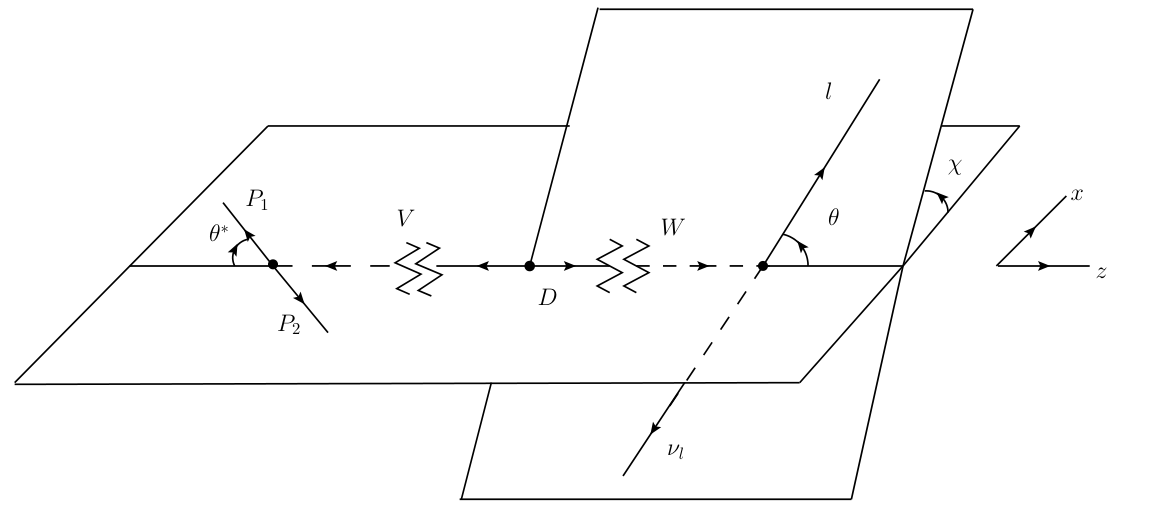
The kinematics for four-body decay is elaborated in Refs. Kang et al. 2014a; Cheng and Kang 2018; Stoffer 2014 and earlier papers Cabibbo and Maksymowicz 1965; Pais and Treiman 1968. As shown in Fig. 2, we define θ\theta as the polar angle of the lepton in the l+​νll^{+}\nu_{l} center-of-mass frame with respect to the Woff-shellW_{\text{off-shell}} line of flight in the DD rest frame. Additionally, θ∗\theta^{*} is defined as the polar angle of P1P_{1} in the VV rest frame with respect to the VV meson line of flight in the DD rest frame. χ\chi is the dihedral angle between the l+​νll^{+}\nu_{l} and the P1​P2P_{1}P_{2} planes. The zz-axis is along the momentum direction of Woff-shellW_{\text{off-shell}} in the DD rest frame, and the momenta of P1P_{1} and P2P_{2} lie in the x​zxz plane.

Refer to caption

Figure 2: The definitions of θ\theta, θ∗\theta^{*} and the azimuthal angle χ\chi.

In the rest frame of final meson VV, the corresponding momenta are

p2μ\displaystyle p_{2}^{\mu} =(m2,0,0,0),\displaystyle=\left(m_{2},0,0,0\right), (22)
p3μ\displaystyle p_{3}^{\mu} =(E3,|p→3|sinθ∗,0,−|p→3|cosθ∗),\displaystyle=\left(E_{3},|\vec{p}_{3}|\sin\theta^{*},0,-|\vec{p}_{3}|\cos\theta^{*}\right),
p4μ\displaystyle p_{4}^{\mu} =(E4,−|p→3|sinθ∗,0,|p→3|cosθ∗),\displaystyle=\left(E_{4},-|\vec{p}_{3}|\sin\theta^{*},0,|\vec{p}_{3}|\cos\theta^{*}\right),

and the polarization vectors of VV meson are

ϵ2μ​(+)=12​(0,+1,−i,0),ϵ2μ​(−)=12​(0,−1,−i,0),ϵ2μ​(0)=(0,0,0,−1).\epsilon_{2}^{\mu}(+)=\frac{1}{\sqrt{2}}\left(0,+1,-i,0\right),\;\epsilon_{2}^{\mu}(-)=\frac{1}{\sqrt{2}}\left(0,-1,-i,0\right),\;\epsilon_{2}^{\mu}(0)=\left(0,0,0,-1\right). (23)

In the decay process of D→V(→P1P2)lνlD\to V(\to P_{1}P_{2})l\nu_{l}, the hadronic tensor is given by

H⁡(λW,λW′)\displaystyle H\left(\lambda_{W},\lambda_{W}^{\prime}\right) =ϵ†μ​(λW)​ϵν​(λW′)​Hμ​ν\displaystyle=\epsilon^{\dagger\mu}(\lambda_{W})\epsilon^{\nu}(\lambda_{W}^{\prime})H_{\mu\nu} (24)
=ϵ†μ​(λW)​ϵν​(λW′)​ϵ2†α​(λV)​ϵ2β​(λV′)​Tμ​α​(Tν​β)†​gV​P​P2​p3​α′​p3​β′​ϵ2α′​(λV)​ϵ2†β′​(λV′)\displaystyle=\epsilon^{\dagger\mu}(\lambda_{W})\epsilon^{\nu}(\lambda_{W}^{\prime})\epsilon_{2}^{\dagger\alpha}(\lambda_{V})\epsilon_{2}^{\beta}(\lambda_{V}^{\prime})T_{\mu\alpha}(T_{\nu\beta})^{\dagger}g^{2}_{VPP}p_{3\alpha^{\prime}}p_{3\beta^{\prime}}\epsilon_{2}^{\alpha^{\prime}}(\lambda_{V})\epsilon_{2}^{\dagger\beta^{\prime}}(\lambda_{V}^{\prime})
=gV​P​P2​p3​α′​p3​β′​ϵ2α′​(λV)​ϵ2†β′​(λV′)×HλW,λV​HλW′,λV′†,\displaystyle=g^{2}_{VPP}p_{3\alpha^{\prime}}p_{3\beta^{\prime}}\epsilon_{2}^{\alpha^{\prime}}(\lambda_{V})\epsilon_{2}^{\dagger\beta^{\prime}}(\lambda_{V}^{\prime})\times H_{\lambda_{W},\lambda_{V}}H^{\dagger}_{\lambda_{W}^{\prime},\lambda_{V}^{\prime}},

where gV​P​P⋅ϵ2ρ​(λV)⋅p3​ρg_{VPP}\cdot\epsilon_{2}^{\rho}(\lambda_{V})\cdot p_{3\rho} describes the amplitude 𝒜⁡(V→P1​P2)\mathcal{A}(V\to P_{1}P_{2}), and the effective coupling constant gV​P​Pg_{VPP} is related to the branching ratio B​r​(V→P1​P2)Br(V\to P_{1}P_{2}) by

gV​P​P2=24​π​m22​ΓV​B​r|p→3|3,g^{2}_{VPP}=\frac{24\pi m_{2}^{2}\Gamma_{V}Br}{|\vec{p}_{3}|^{3}}, (25)

with ΓV\Gamma_{V} being the finite width of vector meson. Notice that Sα​α′​(p2)=∑λV=±1,0ϵ2α​(λV)​ϵ2†α′​(λV)S^{\alpha\alpha^{\prime}}(p_{2})=\displaystyle\sum_{\lambda_{V}=\pm 1,0}\epsilon_{2}^{\alpha}(\lambda_{V})\epsilon_{2}^{\dagger\alpha^{\prime}}(\lambda_{V}) is just the numerator of the propagator of intermediate meson VV. Additionally, Eq. (24) agrees with Eq. (37) in Ref. Ivanov et al. 2019, except for some extra factors that will be compensated in the final result.

III THE TWOFOLD AND FOURFOLD DIFFERENTIAL DECAY DISTRIBUTIONS

In this section, we consider the differential decay distribution. For the D→P⁡(V)​l+​νlD\rightarrow P(V)l^{+}\nu_{l} transition, we have

d2​Γ​(D→P⁡(V)​l+​νl)d​q2​d​cos⁡θ=|p→2|(2​π)3​32​m12​(1−ml2q2)​∑spins|ℳ|2=GF2​|Vc​q|2(2​π)3​|p→2|64​m12​(1−ml2q2)​L​(λW,λW′)​gλW​λW′′​gλW′​λW′′′​H​(λW′′,λW′′′),\begin{split}\frac{d^{2}\Gamma(D\rightarrow P(V)l^{+}\nu_{l})}{dq^{2}d\cos\theta}&=\frac{|\vec{p}_{2}|}{(2\pi)^{3}32m_{1}^{2}}\left(1-\frac{m_{l}^{2}}{q^{2}}\right)\sum\limits_{\text{spins}}\left|\mathcal{M}\right|^{2}\\ &=\frac{G_{F}^{2}|V_{cq}|^{2}}{(2\pi)^{3}}\frac{|\vec{p}_{2}|}{64m_{1}^{2}}\left(1-\frac{m_{l}^{2}}{q^{2}}\right)L\left(\lambda_{W},\lambda_{W}^{\prime}\right)g_{\lambda_{W}\lambda_{W}^{\prime\prime}}g_{\lambda_{W}^{\prime}\lambda_{W}^{\prime\prime\prime}}H\left(\lambda_{W}^{\prime\prime},\lambda_{W}^{\prime\prime\prime}\right),\end{split} (26)

where mlm_{l} is the lepton mass, and the factor in front of |ℳ|2|\mathcal{M}|^{2} corresponds to the three-body phase factor. In terms of the helicity amplitudes, Eqs. (11) and (16), the hadronic tensor is

H⁡(λW,λW′)={HλW​HλW′†,D→P,HλW​λV​HλW′​λV†,D→V.H\left(\lambda_{W},\lambda_{W}^{\prime}\right)=\begin{cases}H_{\lambda_{W}}H_{\lambda_{W}^{\prime}}^{\dagger},\quad\quad\quad\quad D\rightarrow P,\\ H_{\lambda_{W}\lambda_{V}}H_{\lambda_{W}^{\prime}\lambda_{V}}^{\dagger},\quad\quad D\rightarrow V.\end{cases} (27)

We then evaluate the leptonic tensor L⁡(λW,λW′)=ϵμ​(λW)​ϵ†ν​(λW′)​Lμ​νL(\lambda_{W},\lambda_{W}^{\prime})=\epsilon^{\mu}(\lambda_{W})\epsilon^{\dagger\nu}(\lambda_{W}^{\prime})L_{\mu\nu}. The leptonic tensor can be given by

Lμ​ν={tr​[(k̸1+ml)​Oμ​k̸2​Oν],W−→l−​ν¯l,tr​[(k̸1−ml)​Oν​k̸2​Oμ],W+→l+​νl,=8​(k1​μ​k2​ν+k1​ν​k2​μ−k1⋅k2​gμ​ν±i​εμ​ν​α​β​k1α​k2β),\begin{split}L_{\mu\nu}&=\begin{cases}\text{tr}\left[\left(\not{k}_{1}+m_{l}\right)O_{\mu}\not{k}_{2}O_{\nu}\right],\quad\quad W^{-}\rightarrow l^{-}\bar{\nu}_{l},\\ \text{tr}\left[\left(\not{k}_{1}-m_{l}\right)O_{\nu}\not{k}_{2}O_{\mu}\right],\quad\quad W^{+}\rightarrow l^{+}\nu_{l},\end{cases}\\ &=8\left(k_{1\mu}k_{2\nu}+k_{1\nu}k_{2\mu}-k_{1}\cdot k_{2}g_{\mu\nu}\pm i\varepsilon_{\mu\nu\alpha\beta}k_{1}^{\alpha}k_{2}^{\beta}\right),\end{split} (28)

where k1,k2k_{1},k_{2} denote the momentum of a charged lepton and neutrino, respectively. The evaluation of the leptonic tensor is performed in the Woff-shellW_{\text{off-shell}} rest frame, and the explicit expressions of the momentum can be written as

qμ=(q2,0,0,0),k1μ=(E1,|k→1|​sin⁡θ​cos⁡χ,|k→1|​sin⁡θ​sin⁡χ,|k→1|​cos⁡θ),k2μ=(|k→1|,−|k→1|​sin⁡θ​cos⁡χ,−|k→1|​sin⁡θ​sin⁡χ,−|k→1|​cos⁡θ),\begin{split}&q^{\mu}=\left(\sqrt{q^{2}},0,0,0\right),\\ &k_{1}^{\mu}=\left(E_{1},|\vec{k}_{1}|\sin\theta\cos\chi,|\vec{k}_{1}|\sin\theta\sin\chi,|\vec{k}_{1}|\cos\theta\right),\\ &k_{2}^{\mu}=\left(|\vec{k}_{1}|,-|\vec{k}_{1}|\sin\theta\cos\chi,-|\vec{k}_{1}|\sin\theta\sin\chi,-|\vec{k}_{1}|\cos\theta\right),\end{split} (29)

where E1=(q2+ml2)/2​q2E_{1}=\left(q^{2}+m_{l}^{2}\right)/2\sqrt{q^{2}} is the energy and |k1→|=(q2−ml2)/2​q2|\vec{k_{1}}|=\left(q^{2}-m_{l}^{2}\right)/2\sqrt{q^{2}} is the three-momentum of the lepton. The polarization vectors of WW in this rest frame are given by

ϵμ​(0)=(0,0,0,1),ϵμ​(±)=12​(0,∓1,−i,0),ϵμ​(t)=(1,0,0,0).\epsilon^{\mu}(0)=\left(0,0,0,1\right),\quad\epsilon^{\mu}(\pm)=\frac{1}{\sqrt{2}}\left(0,\mp 1,-i,0\right),\quad\epsilon^{\mu}(t)=\left(1,0,0,0\right). (30)

Combining the momentum and polarization vectors, Eqs. (28)-(30), we obtain the expression for L⁡(λW,λW′)L(\lambda_{W},\lambda_{W}^{\prime}), where the matrix columns and rows are ordered in the sequence (t,+,0,−)(t,+,0,-) (In Ref. Ivanov et al. 2019, the element in the first row and second column of the matrix after δ\delta contains a typo, χ\chi should be replaced by χ\chi):

(2​q2​v)−1​L​(λW,λW′)​(θ,χ)\displaystyle(2q^{2}v)^{-1}L(\lambda_{W},\lambda_{W}^{\prime})(\theta,\chi) =(00000(1∓cos⁡θ)2∓22​(1∓cos⁡θ)​sin⁡θ​ei​χsin2⁡θ​e2​i​χ0∓22​(1∓cos⁡θ)​sin⁡θ​e−i​χ2​sin2⁡θ∓22​(1±cos⁡θ)​sin⁡θ​ei​χ0sin2⁡θ​e−2​i​χ∓22​(1±cos⁡θ)​sin⁡θ​e−i​χ(1±cos⁡θ)2)\displaystyle=\left(\begin{array}[]{cccc}0&0&0&0\\ 0&(1\mp\cos\theta)^{2}&\mp\frac{2}{\sqrt{2}}(1\mp\cos\theta)\sin\theta e^{i\chi}&\sin^{2}\theta e^{2i\chi}\\ 0&\mp\frac{2}{\sqrt{2}}(1\mp\cos\theta)\sin\theta e^{-i\chi}&2\sin^{2}\theta&\mp\frac{2}{\sqrt{2}}(1\pm\cos\theta)\sin\theta e^{i\chi}\\ 0&\sin^{2}\theta e^{-2i\chi}&\mp\frac{2}{\sqrt{2}}(1\pm\cos\theta)\sin\theta e^{-i\chi}&(1\pm\cos\theta)^{2}\end{array}\right) (31)
+δl​(4−42​sin⁡θ​e−i​χ4​cos⁡θ42​sin⁡θ​ei​χ−42​sin⁡θ​ei​χ2​sin2⁡θ−22​sin⁡2​θ​ei​χ−2​sin2⁡θ​e2​i​χ4​cos⁡θ−22​sin⁡2​θ​e−i​χ4​cos2⁡θ22​sin⁡2​θ​ei​χ42​sin⁡θ​e−i​χ−2​sin2⁡θ​e−2​i​χ22​sin⁡2​θ​e−i​χ2​sin2⁡θ).\displaystyle+\delta_{l}\left(\begin{array}[]{cccc}4&-\frac{4}{\sqrt{2}}\sin\theta e^{-i\chi}&4\cos\theta&\frac{4}{\sqrt{2}}\sin\theta e^{i\chi}\\ -\frac{4}{\sqrt{2}}\sin\theta e^{i\chi}&2\sin^{2}\theta&-\frac{2}{\sqrt{2}}\sin 2\theta e^{i\chi}&-2\sin^{2}\theta e^{2i\chi}\\ 4\cos\theta&-\frac{2}{\sqrt{2}}\sin 2\theta e^{-i\chi}&4\cos^{2}\theta&\frac{2}{\sqrt{2}}\sin 2\theta e^{i\chi}\\ \frac{4}{\sqrt{2}}\sin\theta e^{-i\chi}&-2\sin^{2}\theta e^{-2i\chi}&\frac{2}{\sqrt{2}}\sin 2\theta e^{-i\chi}&2\sin^{2}\theta\end{array}\right).

where the upper/lower sign refers to the (l−​ν¯l)/(l+​νl)(l^{-}\bar{\nu}_{l})/(l^{+}\nu_{l}) configuration. To obtain the distribution on the polar angular θ\theta, we integrate over the azimuthal angel χ\chi, and then, the matrix becomes

(2​q2​v)−1​L​(λW,λW′)​(θ)=(00000(1∓cos⁡θ)200002​sin2⁡θ0000(1±cos⁡θ)2)+δl​(404​cos⁡θ002​sin2⁡θ004​cos⁡θ04​cos2⁡θ00002​sin2⁡θ),(2q^{2}v)^{-1}L(\lambda_{W},\lambda_{W}^{\prime})(\theta)=\left(\begin{array}[]{cccc}0&0&0&0\\ 0&(1\mp\cos\theta)^{2}&0&0\\ 0&0&2\sin^{2}\theta&0\\ 0&0&0&(1\pm\cos\theta)^{2}\end{array}\right)+\delta_{l}\left(\begin{array}[]{cccc}4&0&4\cos\theta&0\\ 0&2\sin^{2}\theta&0&0\\ 4\cos\theta&0&4\cos^{2}\theta&0\\ 0&0&0&2\sin^{2}\theta\end{array}\right), (32)

where v=1−ml2/q2v=1-m_{l}^{2}/q^{2} is the velocity-type parameter and δl=ml2/2​q2\delta_{l}=m_{l}^{2}/2q^{2} is the helicity-flip factor.

We consider now the circumstance of W+→l+​νlW^{+}\rightarrow l^{+}\nu_{l}, and the W−→l−​ν¯lW^{-}\rightarrow l^{-}\bar{\nu}_{l} case will be discussed later. Combing the Eq. (32) and Eq. (27), one has the contraction Hμ​ν​Lμ​ν​(θ)H^{\mu\nu}L_{\mu\nu}(\theta) in helicity amplitude space as follows:

Hμ​ν​Lμ​ν​(θ)=L⁡(λW,λW′)​gλW​λW′′​gλW′​λW′′′​H​(λW′′,λW′′′)=(2q2v)×{[(1+cos2θ)+2δlsin2θ](|H+|2+|H−|2)+(2sin2θ+4δlcos2θ)|H0|2+2cosθ(|H+|2−|H−|2)+4δl|Ht|2−8δlcosθRe(H0Ht†)}=(2q2v)×[(1+cos2θ)ℋU+2sin2θℋL+2cosθℋP+2δl(sin2θℋU+2cos2θℋL+2ℋS−4cosθℋS​L)].\begin{split}H^{\mu\nu}L_{\mu\nu}(\theta)=&L\left(\lambda_{W},\lambda_{W}^{\prime}\right)g_{\lambda_{W}\lambda_{W}^{\prime\prime}}g_{\lambda_{W}^{\prime}\lambda_{W}^{\prime\prime\prime}}H\left(\lambda_{W}^{\prime\prime},\lambda_{W}^{\prime\prime\prime}\right)\\ =&\left(2q^{2}v\right)\times\left\{\left[\left(1+\cos^{2}\theta\right)+2\delta_{l}\sin^{2}\theta\right]\left(\left|H_{+}\right|^{2}+\left|H_{-}\right|^{2}\right)+\left(2\sin^{2}\theta+4\delta_{l}\cos^{2}\theta\right)\left|H_{0}\right|^{2}\right.\\ &\left.+2\cos\theta\left(\left|H_{+}\right|^{2}-\left|H_{-}\right|^{2}\right)+4\delta_{l}\left|H_{t}\right|^{2}-8\delta_{l}\cos\theta\,\text{Re}\left(H_{0}H_{t}^{\dagger}\right)\right\}\\ =&\left(2q^{2}v\right)\times\left[\left(1+\cos^{2}\theta\right)\mathcal{H}_{U}+2\sin^{2}\theta\mathcal{H}_{L}+2\cos\theta\mathcal{H}_{P}\right.\\ &\left.+2\delta_{l}\left(\sin^{2}\theta\mathcal{H}_{U}+2\cos^{2}\theta\mathcal{H}_{L}+2\mathcal{H}_{S}-4\cos\theta\mathcal{H}_{SL}\right)\right].\end{split} (33)

The above equation contains relevant bilinear combinations ℋi\mathcal{H}_{i}, called by the helicity structure functions Ivanov et al. 2015, whose definitions are listed in Table 1.

Table 1: Definitions of helicity structure functions
Parity-conserving Parity-violating
ℋU=|H+|2+|H−|2\mathcal{H}_{U}=|H_{+}|^{2}+|H_{-}|^{2} ℋP=|H+|2−|H−|2\mathcal{H}_{P}=|H_{+}|^{2}-|H_{-}|^{2}
ℋL=|H0|2\mathcal{H}_{L}=|H_{0}|^{2} ℋA=12​Re​(H+​H0†−H−​H0†)\mathcal{H}_{A}=\frac{1}{2}\text{Re}(H_{+}H_{0}^{\dagger}-H_{-}H_{0}^{\dagger})
ℋT=Re​(H+​H−†)\mathcal{H}_{T}=\text{Re}(H_{+}H_{-}^{\dagger}) ℋI​A=12​Im​(H+​H0†−H−​H0†)\mathcal{H}_{IA}=\frac{1}{2}\text{Im}(H_{+}H_{0}^{\dagger}-H_{-}H_{0}^{\dagger})
ℋI​T=Im​(H+​H−†)\mathcal{H}_{IT}=\text{Im}(H_{+}H_{-}^{\dagger}) ℋS​A=12​Re​(H+​Ht†−H−​Ht†)\mathcal{H}_{SA}=\frac{1}{2}\text{Re}(H_{+}H_{t}^{\dagger}-H_{-}H_{t}^{\dagger})
ℋI=12​Re​(H+​H0†+H−​H0†)\mathcal{H}_{I}=\frac{1}{2}\text{Re}(H_{+}H_{0}^{\dagger}+H_{-}H_{0}^{\dagger}) ℋI​S​A=12​Im​(H+​Ht†−H−​Ht†)\mathcal{H}_{ISA}=\frac{1}{2}\text{Im}(H_{+}H_{t}^{\dagger}-H_{-}H_{t}^{\dagger})
ℋI​I=12​Im​(H+​H0†+H−​H0†)\mathcal{H}_{II}=\frac{1}{2}\text{Im}(H_{+}H_{0}^{\dagger}+H_{-}H_{0}^{\dagger})
ℋS=|Ht|2\mathcal{H}_{S}=|H_{t}|^{2}
ℋS​T=12​Re​(H+​Ht†+H−​Ht†)\mathcal{H}_{ST}=\frac{1}{2}\text{Re}(H_{+}H_{t}^{\dagger}+H_{-}H_{t}^{\dagger})
ℋI​S​T=12​Im​(H+​Ht†+H−​Ht†)\mathcal{H}_{IST}=\frac{1}{2}\text{Im}(H_{+}H_{t}^{\dagger}+H_{-}H_{t}^{\dagger})
ℋS​L=Re​(H0​Ht†)\mathcal{H}_{SL}=\text{Re}(H_{0}H_{t}^{\dagger})
ℋI​S​L=Im​(H0​Ht†)\mathcal{H}_{ISL}=\text{Im}(H_{0}H_{t}^{\dagger})
ℋt​o​t=ℋU+ℋL+δl​(ℋU+ℋL+3​ℋS)\mathcal{H}_{tot}=\mathcal{H}_{U}+\mathcal{H}_{L}+\delta_{l}\left(\mathcal{H}_{U}+\mathcal{H}_{L}+3\mathcal{H}_{S}\right)

Then, we obtain the twofold differential decay distribution on q2q^{2} and cos⁡θ\cos\theta:

d​Γ​(D→P⁡(V)​l+​νl)d​q2​d​cos⁡θ=GF2​|Vc​q|2​|p→2|​q2​v232​(2​π)3​m12×[(1+cos2θ)ℋU+2sin2θℋL+2cosθℋP+2δl(sin2θℋU+2cos2θℋL+2ℋS−4cosθℋS​L)].\begin{split}\frac{d\Gamma\left(D\rightarrow P(V)l^{+}\nu_{l}\right)}{dq^{2}d\cos\theta}=&\frac{G_{F}^{2}|V_{cq}|^{2}|\vec{p}_{2}|q^{2}v^{2}}{32(2\pi)^{3}m_{1}^{2}}\times\left[\left(1+\cos^{2}\theta\right)\mathcal{H}_{U}+2\sin^{2}\theta\mathcal{H}_{L}+2\cos\theta\mathcal{H}_{P}\right.\\ &\left.+2\delta_{l}\left(\sin^{2}\theta\mathcal{H}_{U}+2\cos^{2}\theta\mathcal{H}_{L}+2\mathcal{H}_{S}-4\cos\theta\mathcal{H}_{SL}\right)\right].\end{split} (34)

Further integrating over cos⁡θ\cos\theta, the differential q2q^{2} distribution will be

d​Γ​(D→P⁡(V)​l+​νl)d​q2=\displaystyle\frac{d\Gamma\left(D\rightarrow P(V)l^{+}\nu_{l}\right)}{dq^{2}}= GF2​|Vc​q|2​|p→2|​q2​v212​(2​π)3​m12×ℋt​o​t,\displaystyle\frac{G_{F}^{2}|V_{cq}|^{2}|\vec{p}_{2}|q^{2}v^{2}}{12(2\pi)^{3}m_{1}^{2}}\times\mathcal{H}_{tot}, (35)

with ℋt​o​t=ℋU+ℋL+δl​(ℋU+ℋL+3​ℋS)\mathcal{H}_{tot}=\mathcal{H}_{U}+\mathcal{H}_{L}+\delta_{l}\left(\mathcal{H}_{U}+\mathcal{H}_{L}+3\mathcal{H}_{S}\right).

For the cascade decays, we need to consider the fourfold distribution. Equation (24) shows the hadronic tensor, including the cascade decay. Combining the momenta of P1P_{1} Eq. (22) and the polarization vectors of VV meson Eq. (23), the hadronic tensor in the helicity space can be written as

1gV​P​P2​|p→3|2​H​(λW,λW′)=\displaystyle\frac{1}{g^{2}_{VPP}|\vec{p}_{3}|^{2}}H\left(\lambda_{W},\lambda_{W}^{\prime}\right)= (cos2⁡θ∗​|Ht|212​2​sin⁡2​θ∗​Ht​H+†cos2⁡θ∗​Ht​H0†−12​2​sin⁡2​θ∗​Ht​H−†12​2​sin⁡2​θ∗​H+​Ht†12​sin2⁡θ∗​|H+|212​2​sin⁡2​θ∗​H+​H0†−12​sin2⁡θ∗​H+​H−†cos2⁡θ∗​H0​Ht†12​2​sin⁡2​θ∗​H0​H+†cos2⁡θ∗​|H0|2−12​2​sin⁡2​θ∗​H0​H−†−12​2​sin⁡2​θ∗​H−​Ht†−12​sin2⁡θ∗​H−​H+†−12​2​sin⁡2​θ∗​H−​H0†12​sin2⁡θ∗​|H−|2),\displaystyle\left(\begin{array}[]{cccc}\cos^{2}\theta^{*}|H_{t}|^{2}&\frac{1}{2\sqrt{2}}\sin 2\theta^{*}H_{t}H_{+}^{\dagger}&\cos^{2}\theta^{*}H_{t}H_{0}^{\dagger}&-\frac{1}{2\sqrt{2}}\sin 2\theta^{*}H_{t}H_{-}^{\dagger}\\ \frac{1}{2\sqrt{2}}\sin 2\theta^{*}H_{+}H_{t}^{\dagger}&\frac{1}{2}\sin^{2}\theta^{*}|H_{+}|^{2}&\frac{1}{2\sqrt{2}}\sin 2\theta^{*}H_{+}H_{0}^{\dagger}&-\frac{1}{2}\sin^{2}\theta^{*}H_{+}H_{-}^{\dagger}\\ \cos^{2}\theta^{*}H_{0}H_{t}^{\dagger}&\frac{1}{2\sqrt{2}}\sin 2\theta^{*}H_{0}H_{+}^{\dagger}&\cos^{2}\theta^{*}|H_{0}|^{2}&-\frac{1}{2\sqrt{2}}\sin 2\theta^{*}H_{0}H_{-}^{\dagger}\\ -\frac{1}{2\sqrt{2}}\sin 2\theta^{*}H_{-}H_{t}^{\dagger}&-\frac{1}{2}\sin^{2}\theta^{*}H_{-}H_{+}^{\dagger}&-\frac{1}{2\sqrt{2}}\sin 2\theta^{*}H_{-}H_{0}^{\dagger}&\frac{1}{2}\sin^{2}\theta^{*}|H_{-}|^{2}\end{array}\right), (36)

with the matrix orders λW,λW′=t,+,0,−\lambda_{W},\lambda_{W}^{\prime}=t,+,0,-.

The four-body phase space for D→V(→P1P2)lνlD\to V(\to P_{1}P_{2})l\nu_{l} depends on five variables: P1​P2P_{1}P_{2} invariant mass squared ss, l​νll\nu_{l} invariant mass squared q2q^{2}, the angles θ\theta, θ∗\theta^{*} and χ\chi. See the definitions in Fig. 2. Considering the narrow width approximation

1(s−m22)2+m22​ΓV2→ΓV→0πm2​ΓV​δ​(s−m22)\frac{1}{(s-m_{2}^{2})^{2}+m_{2}^{2}\Gamma_{V}^{2}}\xrightarrow{\Gamma_{V}\to 0}\frac{\pi}{m_{2}\Gamma_{V}}\delta(s-m_{2}^{2}) (37)

in the four-body phase space integral, one arrives at

dΓ(D→V(→P1P2)l+νl)dq2dcosθdχdcosθ∗=3​GF2​|Vc​q|2​v​|p→2|(2​π)4​128​m12​B​r​(V→P1​P2)​1|p→3|2​H​(λW,λW′)​L​(λW,λW′),\frac{d\Gamma\left(D\rightarrow V(\rightarrow P_{1}P_{2})l^{+}\nu_{l}\right)}{dq^{2}d\cos\theta d\chi d\cos\theta^{*}}=\frac{3G_{F}^{2}|V_{cq}|^{2}v|\vec{p}_{2}|}{(2\pi)^{4}128m_{1}^{2}}Br(V\to P_{1}P_{2})\frac{1}{|\vec{p}_{3}|^{2}}H(\lambda_{W},\lambda_{W}^{\prime})L(\lambda_{W},\lambda_{W}^{\prime}), (38)

which is then generally expressed as

dΓ(D→V(→P1P2)l+νl)dq2dcosθdχ2​πdcosθ∗=GF2​|Vc​q|2​|p→2|​q2​v212​(2​π)3​m12​B​r​(V→P1​P2)​W​(θ,θ∗,χ),\frac{d\Gamma\left(D\rightarrow V(\rightarrow P_{1}P_{2})l^{+}\nu_{l}\right)}{dq^{2}d\cos\theta d\frac{\chi}{2\pi}d\cos\theta^{*}}=\frac{G_{F}^{2}|V_{cq}|^{2}|\vec{p}_{2}|q^{2}v^{2}}{12(2\pi)^{3}m_{1}^{2}}Br(V\rightarrow P_{1}P_{2})W(\theta,\theta^{*},\chi), (39)

and the angular distribution W⁡(θ,θ∗,χ)W(\theta,\theta^{*},\chi) is given by

W⁡(θ,θ∗,χ)=\displaystyle W\left(\theta,\theta^{*},\chi\right)= 932​(1+cos2⁡θ)​sin2⁡θ∗​ℋU+98​sin2⁡θ​cos2⁡θ∗​ℋL+916​cos⁡θ​sin2⁡θ∗​ℋP\displaystyle\frac{9}{32}\left(1+\cos^{2}\theta\right)\sin^{2}\theta^{*}\mathcal{H}_{U}+\frac{9}{8}\sin^{2}\theta\cos^{2}\theta^{*}\mathcal{H}_{L}+\frac{9}{16}\cos\theta\sin^{2}\theta^{*}\mathcal{H}_{P} (40)
−916​sin2⁡θ​sin2⁡θ∗​cos⁡2​χ​ℋT+98​sin⁡θ​sin⁡2​θ∗​cos⁡χ​ℋA\displaystyle-\frac{9}{16}\sin^{2}\theta\sin^{2}\theta^{*}\cos 2\chi\mathcal{H}_{T}+\frac{9}{8}\sin\theta\sin 2\theta^{*}\cos\chi\mathcal{H}_{A}
+916​sin⁡2​θ​sin⁡2​θ∗​cos⁡χ​ℋI−98​sin⁡θ​sin⁡2​θ∗​sin⁡χ​ℋI​I\displaystyle+\frac{9}{16}\sin 2\theta\sin 2\theta^{*}\cos\chi\mathcal{H}_{I}-\frac{9}{8}\sin\theta\sin 2\theta^{*}\sin\chi\mathcal{H}_{II}
−916​sin⁡2​θ​sin⁡2​θ∗​sin⁡χ​ℋI​A+916​sin2⁡θ​sin2⁡θ∗​sin⁡2​χ​ℋI​T\displaystyle-\frac{9}{16}\sin 2\theta\sin 2\theta^{*}\sin\chi\mathcal{H}_{IA}+\frac{9}{16}\sin^{2}\theta\sin^{2}\theta^{*}\sin 2\chi\mathcal{H}_{IT}
+\displaystyle+ δl[94cos2θ∗ℋS−92cosθcos2θ∗ℋS​L+94cos2θcos2θ∗ℋL\displaystyle\delta_{l}\left[\frac{9}{4}\cos^{2}\theta^{*}\mathcal{H}_{S}-\frac{9}{2}\cos\theta\cos^{2}\theta^{*}\mathcal{H}_{SL}+\frac{9}{4}\cos^{2}\theta\cos^{2}\theta^{*}\mathcal{H}_{L}\right.
+916​sin2⁡θ​sin2⁡θ∗​ℋU+98​sin2⁡θ​sin2⁡θ∗​cos⁡2​χ​ℋT\displaystyle+\frac{9}{16}\sin^{2}\theta\sin^{2}\theta^{*}\mathcal{H}_{U}+\frac{9}{8}\sin^{2}\theta\sin^{2}\theta^{*}\cos 2\chi\mathcal{H}_{T}
+94​sin⁡θ​sin⁡2​θ∗​cos⁡χ​ℋS​T−98​sin⁡2​θ​sin⁡2​θ∗​cos⁡χ​ℋI\displaystyle+\frac{9}{4}\sin\theta\sin 2\theta^{*}\cos\chi\mathcal{H}_{ST}-\frac{9}{8}\sin 2\theta\sin 2\theta^{*}\cos\chi\mathcal{H}_{I}
−94​sin⁡θ​sin⁡2​θ∗​sin⁡χ​ℋI​S​A+98​sin⁡2​θ​sin⁡2​θ∗​sin⁡χ​ℋI​A\displaystyle-\frac{9}{4}\sin\theta\sin 2\theta^{*}\sin\chi\mathcal{H}_{ISA}+\frac{9}{8}\sin 2\theta\sin 2\theta^{*}\sin\chi\mathcal{H}_{IA}
−98sin2θsin2θ∗sin2χℋI​T].\displaystyle\left.-\frac{9}{8}\sin^{2}\theta\sin^{2}\theta^{*}\sin 2\chi\mathcal{H}_{IT}\right].

Note that the observables such as differential decay rate, forward-backward asymmetry, polarization of τ\tau and vector mesons, can be constructed from three-body decays directly, without the help of Eq. (40), which is derived assuming the narrow width limit. The uncertainty due to the narrow width approximation influence only the following WiW_{i} measurements. Even so, the finite-width effect is generally very small for vector menson, less than a few percent, as explored in Ref. Cheng et al. 2020.

IV THE PHYSICAL OBSERVABLES

To study the effect of the lepton mass and provide a more detailed physical picture in semileptonic decays beyond the branching fraction, we can also define other physical observables that can be measured experimentally, such as forward-backward asymmetry (𝒜F​Bl)\left(\mathcal{A}_{FB}^{l}\right), longitudinal (PLl)\left(P_{L}^{l}\right) and transverse (PTl)\left(P_{T}^{l}\right) polarization of the charged lepton, longitudinal polarization (FLl​(V))\left(F_{L}^{l}(V)\right) of the final vector meson, leptonic convexity parameter (CFl)\left(C_{F}^{l}\right), and trigonometric momentum (Wi)\left(W_{i}\right) in the angular distribution. These observables are expressed again by the above helicity structure functions. The hadronic convexity parameter (CFh)\left(C_{F}^{h}\right) is simply related to the longitudinal polarization of vector, and we will not repetitively calculate CFhC_{F}^{h}.

First, we consider the forward-backward asymmetry. The “forward” region requires the θ∈[0,π/2]\theta\in\left[0,\pi/2\right] and the “backward” region θ∈[π/2,π]\theta\in\left[\pi/2,\pi\right]. Then, 𝒜F​Bl\mathcal{A}_{FB}^{l} is defined as

𝒜F​Bl​(q2)\displaystyle\mathcal{A}_{FB}^{l}(q^{2}) =∫01d​cos⁡θ​d​Γd​q2​d​cos⁡θ−∫−10d​cos⁡θ​d​Γd​q2​d​cos⁡θ∫01d​cos⁡θ​d​Γd​q2​d​cos⁡θ+∫−10d​cos⁡θ​d​Γd​q2​d​cos⁡θ\displaystyle=\frac{\int_{0}^{1}d\cos\theta\frac{d\Gamma}{dq^{2}d\cos\theta}-\int_{-1}^{0}d\cos\theta\frac{d\Gamma}{dq^{2}d\cos\theta}}{\int_{0}^{1}d\cos\theta\frac{d\Gamma}{dq^{2}d\cos\theta}+\int_{-1}^{0}d\cos\theta\frac{d\Gamma}{dq^{2}d\cos\theta}} (41)
=34​HP−4​δl​HS​LHt​o​t.\displaystyle=\frac{3}{4}\frac{H_{P}-4\delta_{l}H_{SL}}{H_{tot}}.

Next, we consider the polarization observables, which can be derived from the three-body decay. We then define a system where the leptons lie in the x​zxz plane, leading to k1=(E1,|k1→|​sin⁡θ, 0,|k1→|​cos⁡θ)k_{1}=\left(E_{1},\;|\vec{k_{1}}|\sin\theta,\;0,\;|\vec{k_{1}}|\cos\theta\right). That is, the observables have no χ\chi dependence and integration over χ\chi trivially gives 2​π2\pi factor. Generally, the expression of the spin four-vector ss is Greiner and Muller 1993

sμ=(k→1⋅s→^ml,s→^+k→1​(k→1⋅s→^)ml​(k10+ml)),s^{\mu}=\left(\frac{\vec{k}_{1}\cdot\hat{\vec{s}}}{m_{l}},\;\hat{\vec{s}}+\frac{\vec{k}_{1}\left(\vec{k}_{1}\cdot\hat{\vec{s}}\right)}{m_{l}\left(k_{1}^{0}+m_{l}\right)}\right), (42)

which can be obtained by imposing a Lorentz transformation to (0,s→)(0,\vec{s}), and s→\vec{s} is a unit vector defining the direction of spin in the rest frame. For the longitudinal polarization of the charged lepton, k→1⋅s→^=|k→1|\vec{k}_{1}\cdot\hat{\vec{s}}=|\vec{k}_{1}|, we obtain the longitudinal polarization vector:

sLμ=1ml​(|k→1|,E1​sin⁡θ, 0,E1​cos⁡θ),s_{L}^{\mu}=\frac{1}{m_{l}}\left(|\vec{k}_{1}|,\;E_{1}\sin\theta,\;0,\;E_{1}\cos\theta\right), (43)

which satisfies sL​μ​sLμ=−1s_{L\mu}s_{L}^{\mu}=-1, sL​μ​k1μ=0s_{L\mu}k_{1}^{\mu}=0.

For the leptonic tensor Lμ​νL_{\mu\nu} in Eq.(28), one sums over the spins in the the product of Dirac spinors, ∑su⁡(p,s)​u¯​(p,s)=(p̸+m)\sum\limits_{s}u(p,s)\bar{u}(p,s)=\left(\not{p}+m\right) and ∑sv⁡(p,s)​v¯​(p,s)=(p̸−m)\sum\limits_{s}v(p,s)\bar{v}(p,s)=\left(\not{p}-m\right). While the lepton is polarized, one has u⁡(p,sL)​u¯​(p,sL)=12​[(p̸+m)​(1+γ5​s̸)]u(p,s_{L})\bar{u}(p,s_{L})=\frac{1}{2}\left[\left(\not{p}+m\right)\left(1+\gamma_{5}\not{s}\right)\right] and v⁡(p,sL)​v¯​(p,sL)=12​[(p̸−m)​(1+γ5​s̸)]v(p,s_{L})\bar{v}(p,s_{L})=\frac{1}{2}\left[\left(\not{p}-m\right)\left(1+\gamma_{5}\not{s}\right)\right]. The expression of the leptonic tensor for the longitudinally polarized lepton is

Lμ​ν​(sL)=4\displaystyle L_{\mu\nu}(s_{L})=4 (k1​μ​k2​ν+k1​ν​k2​μ−k1⋅k2​gμ​ν±i​εμ​ν​α​β​k1α​k2βCLOSE\displaystyle\left(k_{1\mu}k_{2\nu}+k_{1\nu}k_{2\mu}-k_{1}\cdot k_{2}g_{\mu\nu}\pm i\varepsilon_{\mu\nu\alpha\beta}k_{1}^{\alpha}k_{2}^{\beta}\right. (44)
OPEN∓ml​sL​μ​k2​ν∓ml​sL​ν​k2​μ±ml​sL⋅k2​gμ​ν−i​ml​εμ​ν​α​β​sLα​k2β)\displaystyle\left.\mp m_{l}s_{L\mu}k_{2\nu}\mp m_{l}s_{L\nu}k_{2\mu}\pm m_{l}s_{L}\cdot k_{2}g_{\mu\nu}-im_{l}\varepsilon_{\mu\nu\alpha\beta}s_{L}^{\alpha}k_{2}^{\beta}\right)

where the upper/lower sign refers to the (l−​ν¯l)/(l+​νl)(l^{-}\bar{\nu}_{l})/(l^{+}\nu_{l}) configuration. In Ref. Gutsche et al. 2015 the leptonic tensor is written as

Lμ​ν​(sL)=∓8​ml​(sL​μ​k2​ν+sL​ν​k2​μ−sL⋅k2​gμ​ν±i​εμ​ν​α​β​sLα​k2β),L_{\mu\nu}(s_{L})=\mp 8m_{l}\left(s_{L\mu}k_{2\nu}+s_{L\nu}k_{2\mu}-s_{L}\cdot k_{2}g_{\mu\nu}\pm i\varepsilon_{\mu\nu\alpha\beta}s_{L}^{\alpha}k_{2}^{\beta}\right), (45)

i.e., making the replacement k1μ→∓ml​sLμk_{1}^{\mu}\rightarrow\mp m_{l}s_{L}^{\mu} from the unpolarized case. Equations (44) and (45) are equivalent in the sense of L⁡(λW,λW′)L(\lambda_{W},\lambda_{W}^{\prime}), cf. Eq. (10).

With Eq. (45) we obtain the polarized differential decay distribution:

d​Γ​(sL)d​q2\displaystyle\frac{d\Gamma(s_{L})}{dq^{2}} =GF2​|Vc​q|2​|p→2|​q2​v212​(2​π)3​m12​[−3​δl​|Ht|2+(1−δl)​(|H+|2+|H−|2+|H0|2)]\displaystyle=\frac{G_{F}^{2}|V_{cq}|^{2}|\vec{p}_{2}|q^{2}v^{2}}{12(2\pi)^{3}m_{1}^{2}}\left[-3\delta_{l}\left|H_{t}\right|^{2}+\left(1-\delta_{l}\right)\left(|H_{+}|^{2}+|H_{-}|^{2}+|H_{0}|^{2}\right)\right] (46)
=GF2​|Vc​q|2​|p→2|​q2​v212​(2​π)3​m12​[ℋU+ℋL−δl​(ℋU+ℋL+3​ℋS)].\displaystyle=\frac{G_{F}^{2}|V_{cq}|^{2}|\vec{p}_{2}|q^{2}v^{2}}{12(2\pi)^{3}m_{1}^{2}}\left[\mathcal{H}_{U}+\mathcal{H}_{L}-\delta_{l}\left(\mathcal{H}_{U}+\mathcal{H}_{L}+3\mathcal{H}_{S}\right)\right].

The longitudinal polarization of the lepton is then defined as the ratio of polarized decay distribution Eq. (46) to the unpolarized decay distribution Eq. (35):

PLl​(q2)\displaystyle P_{L}^{l}(q^{2}) =ℋU+ℋL−δl​(ℋU+ℋL+3​ℋS)ℋt​o​t\displaystyle=\frac{\mathcal{H}_{U}+\mathcal{H}_{L}-\delta_{l}\left(\mathcal{H}_{U}+\mathcal{H}_{L}+3\mathcal{H}_{S}\right)}{\mathcal{H}_{tot}} (47)

Similarly, one can obtain the definition of the leptonic transverse polarization PTl​(q2)P_{T}^{l}(q^{2}), where the leptonic polarization direction is perpendicular to its momentum direction:

sTμ=(0,s→^T)=(0,cos⁡θ, 0,−sin⁡θ).s_{T}^{\mu}=\left(0,\;\hat{\vec{s}}_{T}\right)=\left(0,\;\cos\theta,\;0,\;-\sin\theta\right). (48)

s→^T\hat{\vec{s}}_{T} is obtained from rotating s→^L=(sin⁡θ,0,cos⁡θ)\hat{\vec{s}}_{L}=(\sin\theta,0,\cos\theta) by π/2\pi/2 in the counterclockwise direction. Making the substitution k1μ→∓ml​sTμk_{1}^{\mu}\rightarrow\mp m_{l}s_{T}^{\mu}, one obtains the transversely polarized leptonic tensor, and the resulting differential decay distribution is

d​Γ​(sT)d​q2\displaystyle\frac{d\Gamma(s_{T})}{dq^{2}} =GF2​|Vc​q|2​|p→2|​q2​v212​(2​π)3​m12​3​π​δl4​2​[−|H+|2+|H−|2−2​Re​(H0​Ht†)]\displaystyle=\frac{G_{F}^{2}|V_{cq}|^{2}|\vec{p}_{2}|q^{2}v^{2}}{12(2\pi)^{3}m_{1}^{2}}\frac{3\pi\sqrt{\delta_{l}}}{4\sqrt{2}}\left[-\left|H_{+}\right|^{2}+\left|H_{-}\right|^{2}-2\text{Re}(H_{0}H_{t}^{\dagger})\right] (49)
=GF2​|Vc​q|2​|p→2|​q2​v212​(2​π)3​m12​3​π​δl4​2​[−ℋP−2​ℋS​L].\displaystyle=\frac{G_{F}^{2}|V_{cq}|^{2}|\vec{p}_{2}|q^{2}v^{2}}{12(2\pi)^{3}m_{1}^{2}}\frac{3\pi\sqrt{\delta_{l}}}{4\sqrt{2}}\left[-\mathcal{H}_{P}-2\mathcal{H}_{SL}\right].

The transverse polarization of lepton will be

PTl​(q2)\displaystyle P_{T}^{l}(q^{2}) =−3​π​δl4​2​ℋP+2​ℋS​Lℋt​o​t.\displaystyle=-\frac{3\pi\sqrt{\delta_{l}}}{4\sqrt{2}}\frac{\mathcal{H}_{P}+2\mathcal{H}_{SL}}{\mathcal{H}_{tot}}. (50)

In addition, the fourfold decay distribution allows us to define more physical quantities. The angular distribution can be normalized as

W~​(θ∗,θ,χ)=W⁡(θ∗,θ,χ)ℋt​o​t.\widetilde{W}\left(\theta^{*},\theta,\chi\right)=\frac{W\left(\theta^{*},\theta,\chi\right)}{\mathcal{H}_{tot}}. (51)

Integrating W⁡(θ∗,θ,χ)W\left(\theta^{*},\theta,\chi\right) over cos⁡θ∗\cos\theta^{*} and χ\chi, one can recover the angular distribution of θ\theta appearing in the D→V​l​νlD\to Vl\nu_{l} transition (Eq. (34)):

W⁡(θ)=\displaystyle W\left(\theta\right)= 38×[(1+2δl)ℋU+2ℋL+4δlℋS+(2ℋP−8δlℋS​L)cosθ\displaystyle\frac{3}{8}\times\left[\left(1+2\delta_{l}\right)\mathcal{H}_{U}+2\mathcal{H}_{L}+4\delta_{l}\mathcal{H}_{S}+\left(2\mathcal{H}_{P}-8\delta_{l}\mathcal{H}_{SL}\right)\cos\theta\right. (52)
+((1−2δl)ℋU−2(1−2δl)ℋL)cos2θ].\displaystyle\left.+((1-2\delta_{l})\mathcal{H}_{U}-2(1-2\delta_{l})\mathcal{H}_{L})\cos^{2}\theta\right].

The normalized angular distribution of θ\theta is then

W~​(θ)=W⁡(θ)ℋt​o​t=a+b​cos⁡θ+c​cos2⁡θ2​(a+c/3),\widetilde{W}(\theta)=\frac{W(\theta)}{\mathcal{H}_{tot}}=\frac{a+b\cos\theta+c\cos^{2}\theta}{2\left(a+c/3\right)}, (53)

where

a\displaystyle a =3/8×[(1+2​δl)​ℋU+2​ℋL+4​δl​ℋS],\displaystyle=3/8\times\left[\left(1+2\delta_{l}\right)\mathcal{H}_{U}+2\mathcal{H}_{L}+4\delta_{l}\mathcal{H}_{S}\right], (54)
b\displaystyle b =3/8×(2​ℋP−8​δl​ℋS​L),\displaystyle=3/8\times\left(2\mathcal{H}_{P}-8\delta_{l}\mathcal{H}_{SL}\right),
c\displaystyle c =3/8×[(1−2​δl)​ℋU−2​(1−2​δl)​ℋL].\displaystyle=3/8\times\left[\left(1-2\delta_{l}\right)\mathcal{H}_{U}-2\left(1-2\delta_{l}\right)\mathcal{H}_{L}\right].

By the above coefficient definition, it is clear that the linear coefficient indicates the forward-backward asymmetry

𝒜F​B​(q2)=b2​(a+c/3)=34​ℋP−4​δl​ℋS​Lℋt​o​t.\mathcal{A}_{FB}(q^{2})=\frac{b}{2\left(a+c/3\right)}=\frac{3}{4}\frac{\mathcal{H}_{P}-4\delta_{l}\mathcal{H}_{SL}}{\mathcal{H}_{tot}}. (55)

The leptonic convexity parameter is defined as

CFl​(q2)\displaystyle C_{F}^{l}(q^{2}) =d2​W~​(θ)d​(cos⁡θ)2=ca+c/3=34​(1−2​δl)​ℋU−2​ℋLℋt​o​t.\displaystyle=\frac{d^{2}\widetilde{W}(\theta)}{d(\cos\theta)^{2}}=\frac{c}{a+c/3}=\frac{3}{4}\left(1-2\delta_{l}\right)\frac{\mathcal{H}_{U}-2\mathcal{H}_{L}}{\mathcal{H}_{tot}}. (56)

In the same manner, we can obtain the θ∗\theta^{*} angular distribution by integrating the W⁡(θ,θ∗,χ)W(\theta,\theta^{*},\chi) over θ\theta and χ\chi:

W⁡(θ∗)=34×[(1+δl)​ℋU+(−(1+δl)​ℋU+2​(1+δl)​ℋL+6​δl​ℋS)​cos2⁡θ∗].\displaystyle W(\theta^{*})=\frac{3}{4}\times\left[\left(1+\delta_{l}\right)\mathcal{H}_{U}+\left(-\left(1+\delta_{l}\right)\mathcal{H}_{U}+2\left(1+\delta_{l}\right)\mathcal{H}_{L}+6\delta_{l}\mathcal{H}_{S}\right)\cos^{2}\theta^{*}\right]. (57)

The normalized θ∗\theta^{*} angular distribution is described by

W~​(θ∗)=W⁡(θ∗)ℋt​o​t=a′+c′​cos2⁡θ∗2​a′+2/3​c′,\widetilde{W}(\theta^{*})=\frac{W(\theta^{*})}{\mathcal{H}_{tot}}=\frac{a^{\prime}+c^{\prime}\cos^{2}\theta^{*}}{2a^{\prime}+2/3c^{\prime}}, (58)

where

a′\displaystyle a^{\prime} =(1+δl)​ℋU\displaystyle=\left(1+\delta_{l}\right)\mathcal{H}_{U} (59)
c′\displaystyle c^{\prime} =−(1+δl)​ℋU+2​(1+δl)​ℋL+6​δl​ℋS.\displaystyle=-\left(1+\delta_{l}\right)\mathcal{H}_{U}+2\left(1+\delta_{l}\right)\mathcal{H}_{L}+6\delta_{l}\mathcal{H}_{S}.

The hadronic convexity parameter can be extracted by taking the second derivative of W~​(θ∗)\widetilde{W}(\theta^{*}) as

CFh​(q2)\displaystyle C^{h}_{F}(q^{2}) =d2​W~​(θ∗)d​(cos⁡θ∗)2=c′a′+c′/3=−32​ℋU−2​ℋL+δl​(ℋU−2​ℋL−6​ℋS)ℋt​o​t.\displaystyle=\frac{d^{2}\widetilde{W}(\theta^{*})}{d(\cos\theta^{*})^{2}}=\frac{c^{\prime}}{a^{\prime}+c^{\prime}/3}=-\frac{3}{2}\frac{\mathcal{H}_{U}-2\mathcal{H}_{L}+\delta_{l}\left(\mathcal{H}_{U}-2\mathcal{H}_{L}-6\mathcal{H}_{S}\right)}{\mathcal{H}_{tot}}. (60)

The longitudinal polarization fraction of the final vector meson is given by

FLl​(q2)\displaystyle F_{L}^{l}(q^{2}) =d​Γ​(λV=0)/d​q2d​Γ/d​q2=(1+δl)​ℋL+3​δl​ℋSℋt​o​t,\displaystyle=\frac{d\Gamma(\lambda_{V}=0)/dq^{2}}{d\Gamma/dq^{2}}=\frac{(1+\delta_{l})\mathcal{H}_{L}+3\delta_{l}\mathcal{H}_{S}}{\mathcal{H}_{tot}}, (61)

and the transverse polarization fraction is FTl​(q2)=1−FLl​(q2)F_{T}^{l}(q^{2})=1-F_{L}^{l}(q^{2}). The hadronic convexity parameter is related to the longitudinal polarization of vector meson by

CFh​(q2)=32​(3​FL​(q2)−1).C_{F}^{h}(q^{2})=\frac{3}{2}(3F_{L}(q^{2})-1). (62)

Moreover, to examine more helicity structure functions in Eq. (40), we can define the trigonometric moments through the normalized angular decay distribution W~​(θ∗,θ,χ)\widetilde{W}(\theta^{*},\theta,\chi)

Wi=∫dcosθdcosθ∗d(χ/2π)Mi(θ,θ∗,χ)W~(θ,θ∗,χ)=⟨Mi(θ,θ∗,χ)⟩.W_{i}=\int d\cos\theta d\cos\theta^{*}d\left(\chi/2\pi\right)M_{i}\left(\theta,\theta^{*},\chi\right)\widetilde{W}\left(\theta,\theta^{*},\chi\right)=\left\langle M_{i}\left(\theta,\theta^{*},\chi\right)\right\rangle. (63)

Some explicit examples include

WT​(q2)\displaystyle W_{T}(q^{2}) =⟨cos⁡2​χ⟩=−12​(1−2​δl)​ℋTℋt​o​t,\displaystyle=\left\langle\cos 2\chi\right\rangle=-\frac{1}{2}\left(1-2\delta_{l}\right)\frac{\mathcal{H}_{T}}{\mathcal{H}_{tot}}, (64)
WI​(q2)\displaystyle W_{I}(q^{2}) =⟨cosθcosθ∗cosχ⟩=9​π2​(1−2​δl)512ℋIℋt​o​t,\displaystyle=\left\langle\cos\theta\cos\theta^{*}\cos\chi\right\rangle=\frac{9\pi^{2}\left(1-2\delta_{l}\right)}{512}\frac{\mathcal{H}_{I}}{\mathcal{H}_{tot}},
WA​(q2)\displaystyle W_{A}(q^{2}) =⟨sinθsinθ∗cosχ⟩=3​π16ℋA+2​δl​ℋS​Tℋt​o​t.\displaystyle=\left\langle\sin\theta\sin\theta^{*}\cos\chi\right\rangle=\frac{3\pi}{16}\frac{\mathcal{H}_{A}+2\delta_{l}\mathcal{H}_{ST}}{\mathcal{H}_{tot}}.

For final mesons being pseudoscalars, the helicity amplitudes H±=0H_{\pm}=0, which leads to vanishing trigonometric moments. Therefore, Eq. (64) is only applied to D→VD\rightarrow V transitions.

In practice, due to the limited statistics in the experiment, we show the average values of all mentioned physical observables. In such a case, we reinstate the phase factor C⁡(q2)=|p2→|​(q2−ml2)2/q2C(q^{2})=\left|\vec{p_{2}}\right|(q^{2}-m_{l}^{2})^{2}/q^{2} in both numerator and denominator and integrate them separately. More explicitly,

⟨𝒜F​Bl⟩=34​∫d​q2​C​(q2)​(ℋP−4​δl​ℋS​L)∫d​q2​C​(q2)​[ℋU+ℋL+δl​(ℋU+ℋL+3​ℋS)].\langle\mathcal{A}_{FB}^{l}\rangle=\frac{3}{4}\frac{{\int}dq^{2}C(q^{2})\left(\mathcal{H}_{P}-4\delta_{l}\mathcal{H}_{SL}\right)}{{\int}dq^{2}C(q^{2})\left[\mathcal{H}_{U}+\mathcal{H}_{L}+\delta_{l}\left(\mathcal{H}_{U}+\mathcal{H}_{L}+3\mathcal{H}_{S}\right)\right]}. (65)

A similar operation holds for all others. We also present the full momentum dependence of 𝒜F​Bl\mathcal{A}_{FB}^{l}, PLlP_{L}^{l} and PTlP_{T}^{l}.

For the case in which the charge of the lepton is negative, i.e., l−​ν¯ll^{-}\bar{\nu}_{l}, the relative sign in Eq. (28) and Eq. (45) will influence the expressions of some observables. To better compare with experimental and other theoretical results, we also give the definitions of forward-backward asymmetry, leptonic longitudinal and transverse polarization in such a case:

𝒜F​B​(q2)=−34​ℋP+4​δl​ℋS​Lℋt​o​t,\displaystyle\mathcal{A}_{FB}(q^{2})=-\frac{3}{4}\frac{\mathcal{H}_{P}+4\delta_{l}\mathcal{H}_{SL}}{\mathcal{H}_{tot}}, (66)
PLl​(q2)=−ℋU+ℋL−δl​(ℋU+ℋL+3​ℋS)ℋt​o​t,\displaystyle P_{L}^{l}(q^{2})=-\frac{\mathcal{H}_{U}+\mathcal{H}_{L}-\delta_{l}\left(\mathcal{H}_{U}+\mathcal{H}_{L}+3\mathcal{H}_{S}\right)}{\mathcal{H}_{tot}},
PTl​(q2)=−3​π​δl4​2​ℋP−2​ℋS​Lℋt​o​t.\displaystyle P_{T}^{l}(q^{2})=-\frac{3\pi\sqrt{\delta_{l}}}{4\sqrt{2}}\frac{\mathcal{H}_{P}-2\mathcal{H}_{SL}}{\mathcal{H}_{tot}}.

The expressions for other observables do not change.

V NUMERICAL RESULTS AND DISCUSSION

In this section, we will calculate the branching fractions of D(s)D_{(s)} and B(s)B_{(s)} to (P,V)​l+​νl(P,V)l^{+}\nu_{l} and the average values of 𝒜F​Bl\mathcal{A}_{FB}^{l}, PLlP_{L}^{l}, PTlP_{T}^{l}, CFlC_{F}^{l}, and WiW_{i}, on the basis of related form factors and the abovementioned helicity amplitudes. The average values for these observables and the q2q^{2} dependence are presented in the tables and figures below.

Concerning the related form factors in these physical quantities equations, we stick to the predictions in the covariant light-front quark model (CLFQM) Cheng et al. 2004; Verma 2012. The momentum dependence of form factors can be parameterized as 22 2 The shape of form factor is generally smooth, and such a parametrization works very accurately. The difference between it and the exact numerical value is less than 3%. However, there are indeed exceptions. See discussions between Eqs. (33) and (34) in Ref. Cheng et al. 2004. For the B⁡(D)→P11B(D)\to{}^{1}P_{1} decays, a new parametrisation is proposed, but it is not relevant to our current study.

F⁡(q2)=F⁡(0)1−a⁡(q2/mD2)+b​(q2/mD2)2.F(q^{2})=\frac{F(0)}{1-a\left(q^{2}/m_{D}^{2}\right)+b\left(q^{2}/m_{D}^{2}\right)^{2}}. (67)

The values of relevant parameters that appear in form factors are listed in Table 2.

For the final state of the D(s)D_{(s)} transitions, the pseudoscalar mesons PP contain η,η′,π0,K0\eta,\eta^{\prime},\pi^{0},K^{0}, K0¯\bar{K^{0}} and the vector mesons VV contain ρ,ω,ϕ,K∗\rho,\omega,\phi,K^{*},K∗¯\bar{K^{*}}; for the B(s)B_{(s)} transitions, the pseudoscalar mesons PP contain η,η′,π0,D¯0,Ds−\eta,\eta^{\prime},\pi^{0},\bar{D}^{0},D_{s}^{-} and the vector mesons VV contain ρ,ω,K∗⁣−,D¯∗0\rho,\omega,K^{*-},\bar{D}^{*0}, Ds∗⁣−D_{s}^{*-}. For η\eta and η′\eta^{\prime}, we need to consider the quark mixing scheme Feldmann et al. 1998; Feldmann 2000

(ηη′)=(cos⁡ϕ−sin⁡ϕsin⁡ϕcos⁡ϕ)​(ηqηs),\left(\begin{array}[]{c}\eta\\ \eta^{\prime}\end{array}\right)=\left(\begin{array}[]{cc}\cos\phi&-\sin\phi\\ \sin\phi&\cos\phi\end{array}\right)\left(\begin{array}[]{c}\eta_{q}\\ \eta_{s}\end{array}\right), (68)

where ηq=12​(μ​μ¯+d​d¯)\eta_{q}=\frac{1}{\sqrt{2}}(\mu\bar{\mu}+d\bar{d}), ηs=s​s¯\eta_{s}=s\bar{s}, and the mixing angle ϕ=39.3∘\phi=39.3^{\circ} from Ref. Zyla et al. 2020; Dai et al. 2018b.

Table 2: The form factor parameters predicted by CLFQM in D(s)/B(s)→P⁡(V)D_{(s)}/B_{(s)}\rightarrow P(V) transitions. The values are taken from Ref. Verma 2012.
FF F⁡(0)F(0) aa bb FF F⁡(0)F(0) aa bb FF F⁡(0)F(0) aa bb FF F⁡(0)F(0) aa bb
F1D​πF_{1}^{D\pi} 0.66 1.19 0.35 F0D​πF_{0}^{D\pi} 0.66 0.51 0.00 F1B​πF_{1}^{B\pi} 0.25 1.70 0.90 F0B​πF_{0}^{B\pi} 0.25 0.82 0.09
F1D​ηqF_{1}^{D\eta_{q}} 0.71 1.13 0.27 F0D​ηqF_{0}^{D\eta_{q}} 0.71 0.43 −0.01-0.01 F1B​ηqF_{1}^{B\eta_{q}} 0.29 1.63 0.74 F0B​ηqF_{0}^{B\eta_{q}} 0.29 0.75 0.04
F1D​KF_{1}^{DK} 0.79 1.05 0.25 F0D​KF_{0}^{DK} 0.79 0.47 −0.00-0.00 F1B​DF_{1}^{BD} 0.67 1.22 0.36 F0B​DF_{0}^{BD} 0.67 0.63 −0.01-0.01
F1Ds​KF_{1}^{D_{s}K} 0.66 1.11 0.48 F0Ds​KF_{0}^{D_{s}K} 0.66 0.56 0.04 F1Bs​KF_{1}^{B_{s}K} 0.23 1.88 1.58 F0Bs​KF_{0}^{B_{s}K} 0.23 1.05 0.35
F1Ds​ηsF_{1}^{D_{s}\eta_{s}} 0.76 1.02 0.40 F0Ds​ηsF_{0}^{D_{s}\eta_{s}} 0.76 0.60 0.04 F1Bs​DsF_{1}^{B_{s}D_{s}} 0.67 1.28 0.52 F0Bs​DsF_{0}^{B_{s}D_{s}} 0.67 0.69 0.070.07
VD​ρV^{D\rho} 0.88 1.23 0.40 A0D​ρA_{0}^{D\rho} 0.69 1.08 0.45 A1D​ρA_{1}^{D\rho} 0.60 0.46 0.01 A2D​ρA_{2}^{D\rho} 0.47 0.89 0.23
VD​ωV^{D\omega} 0.85 1.24 0.45 A0D​ωA_{0}^{D\omega} 0.64 1.08 1.50 A1D​ωA_{1}^{D\omega} 0.58 0.49 0.02 A2D​ωA_{2}^{D\omega} 0.49 0.95 0.28
VD​K∗V^{DK^{*}} 0.98 1.10 0.32 A0D​K∗A_{0}^{DK^{*}} 0.78 1.01 0.34 A1D​K∗A_{1}^{DK^{*}} 0.72 0.45 0.01 A2D​K∗A_{2}^{DK^{*}} 0.60 0.89 0.21
VDs​K∗V^{D_{s}K^{*}} 0.87 1.13 0.69 A0Ds​K∗A_{0}^{D_{s}K^{*}} 0.61 0.90 0.62 A1Ds​K∗A_{1}^{D_{s}K^{*}} 0.56 0.59 0.08 A2Ds​K∗A_{2}^{D_{s}K^{*}} 0.46 0.90 0.43
VDs​ϕV^{D_{s}\phi} 0.98 1.04 0.54 A0Ds​ϕA_{0}^{D_{s}\phi} 0.72 0.92 0.62 A1Ds​ϕA_{1}^{D_{s}\phi} 0.69 0.56 0.07 A2Ds​ϕA_{2}^{D_{s}\phi} 0.59 0.90 0.38
VB​ρV^{B\rho} 0.29 1.77 1.06 A0B​ρA_{0}^{B\rho} 0.32 1.67 1.01 A1B​ρA_{1}^{B\rho} 0.24 0.86 0.15 A2B​ρA_{2}^{B\rho} 0.22 1.56 0.85
VB​ωV^{B\omega} 0.27 1.81 1.18 A0B​ωA_{0}^{B\omega} 0.28 1.62 1.22 A1B​ωA_{1}^{B\omega} 0.23 0.91 0.18 A2B​ωA_{2}^{B\omega} 0.21 1.62 0.97
VB​D∗V^{BD^{*}} 0.77 1.25 0.38 A0B​D∗A_{0}^{BD^{*}} 0.68 1.21 0.36 A1B​D∗A_{1}^{BD^{*}} 0.65 0.60 0.00 A2B​D∗A_{2}^{BD^{*}} 0.61 1.12 0.31
VBs​K∗V^{B_{s}K^{*}} 0.23 2.03 2.27 A0Bs​K∗A_{0}^{B_{s}K^{*}} 0.25 1.95 2.20 A1Bs​K∗A_{1}^{B_{s}K^{*}} 0.19 1.24 0.62 A2Bs​K∗A_{2}^{B_{s}K^{*}} 0.16 1.83 1.85
VBs​Ds∗V^{B_{s}D_{s}^{*}} 0.75 1.37 0.67 A0Bs​Ds∗A_{0}^{B_{s}D_{s}^{*}} 0.66 1.33 0.63 A1Bs​Ds∗A_{1}^{B_{s}D_{s}^{*}} 0.62 0.76 0.13 A2Bs​Ds∗A_{2}^{B_{s}D_{s}^{*}} 0.57 1.25 0.56
Table 3: Branching fraction for the semileptonic decays of D+D^{+} and Ds+D_{s}^{+}, compared to the PDG Zyla et al. 2020 and BESIII{\mathrm{III}} results. All values are in unit of 10−310^{-3}

          ee mode μ\mu mode           CLFQM PDG BESIII{\mathrm{III}} CLFQM PDG BESIII{\mathrm{III}}         D+→PD^{+}\rightarrow P     D+→η​l+​νlD^{+}\rightarrow\eta l^{+}\nu_{l} 1.201.20 1.11±0.071.11\pm 0.07 1.161.16 1.04±0.151.04\pm 0.15 Ablikim 2020a           D+→η′​l+​νlD^{+}\rightarrow\eta^{\prime}l^{+}\nu_{l} 0.1790.179 0.20±0.040.20\pm 0.04 0.1690.169           D+→π0​l+​νlD^{+}\rightarrow\pi^{0}l^{+}\nu_{l} 4.094.09 3.72±0.173.72\pm 0.17 3.63±0.133.63\pm 0.13 Ablikim et al. 2017 4.044.04 3.50±0.153.50\pm 0.15           D+→K¯0​l+​νlD^{+}\rightarrow\bar{K}^{0}l^{+}\nu_{l} 103.2103.2 87.3±1.087.3\pm 1.0 86.0±2.186.0\pm 2.1 Ablikim et al. 2017 100.7100.7 87.6±1.987.6\pm 1.9         D+→VD^{+}\rightarrow V     D+→ρ​l+​νlD^{+}\rightarrow\rho l^{+}\nu_{l} 2.322.32 2.18−0.25+0.172.18^{+0.17}_{-0.25} 2.222.22 2.4±0.42.4\pm 0.4           D+→ω​l+​νlD^{+}\rightarrow\omega l^{+}\nu_{l} 2.072.07 1.69±0.111.69\pm 0.11 1.69±0.111.69\pm 0.11 Ablikim 2020b 1.981.98 1.77±0.291.77\pm 0.29 Ablikim 2020b           D+→K¯∗0​l+​νlD^{+}\rightarrow\bar{K}^{*0}l^{+}\nu_{l} 73.273.2 54.0±1.054.0\pm 1.0 69.369.3 52.7±1.552.7\pm 1.5         Ds+→PD_{s}^{+}\rightarrow P     Ds+→η​l+​νlD_{s}^{+}\rightarrow\eta l^{+}\nu_{l} 21.921.9 23.2±0.823.2\pm 0.8 23.0±3.923.0\pm 3.9 Ablikim et al. 2018 21.521.5 24±5.024\pm 5.0 24.2±5.724.2\pm 5.7 Ablikim et al. 2018           Ds+→η′​l+​νlD_{s}^{+}\rightarrow\eta^{\prime}l^{+}\nu_{l} 8.828.82 8.0±0.78.0\pm 0.7 9.3±3.59.3\pm 3.5 Ablikim et al. 2018 8.418.41 11±5.011\pm 5.0 10.6±6.110.6\pm 6.1 Ablikim et al. 2018           Ds+→K0​l+​νlD_{s}^{+}\rightarrow K^{0}l^{+}\nu_{l} 2.542.54 3.4±0.43.4\pm 0.4 2.492.49         Ds+→VD_{s}^{+}\rightarrow V     Ds+→ϕ​l+​νlD_{s}^{+}\rightarrow\phi l^{+}\nu_{l} 30.730.7 23.9±1.623.9\pm 1.6 22.6±5.422.6\pm 5.4 Ablikim et al. 2018 28.928.9 19.0±5.019.0\pm 5.0 19.4±6.219.4\pm 6.2 Ablikim et al. 2018           Ds+→K∗0​l+​νlD_{s}^{+}\rightarrow K^{*0}l^{+}\nu_{l} 1.901.90 2.15±0.282.15\pm 0.28 1.821.82    

Table 4: Branching fraction for the semileptonic decays of B+B^{+} and BsB_{s}, compared to the PDG Tanabashi et al. 2018 results.
      ee mode PDG (l+​νll^{+}\nu_{l}) τ\tau mode PDG (τ+​ντ\tau^{+}\nu_{\tau})    
    B+→PB^{+}\rightarrow P     B+→η​l+​νlB^{+}\rightarrow\eta l^{+}\nu_{l} 4.96×10−54.96\times 10^{-5} (3.9±0.5)×10−5(3.9\pm 0.5)\times 10^{-5} 3.03×10−53.03\times 10^{-5}    
      B+→η′​l+​νlB^{+}\rightarrow\eta^{\prime}l^{+}\nu_{l} 2.41×10−52.41\times 10^{-5} (2.3±0.8)×10−5(2.3\pm 0.8)\times 10^{-5} 1.28×10−51.28\times 10^{-5}    
      B+→π0​l+​νlB^{+}\rightarrow\pi^{0}l^{+}\nu_{l} 7.20×10−57.20\times 10^{-5} (7.8±0.27)×10−5(7.8\pm 0.27)\times 10^{-5} 4.89×10−54.89\times 10^{-5}    
      B+→D¯0​l+​νlB^{+}\rightarrow\bar{D}^{0}l^{+}\nu_{l} 2.59×10−22.59\times 10^{-2} (2.35±0.09)×10−2(2.35\pm 0.09)\times 10^{-2} 0.78×10−20.78\times 10^{-2} (0.77±0.25)×10−2(0.77\pm 0.25)\times 10^{-2}    
    B+→VB^{+}\rightarrow V     B+→ρ​l+​νlB^{+}\rightarrow\rho l^{+}\nu_{l} 2.00×10−42.00\times 10^{-4} (1.58±0.11)×10−4(1.58\pm 0.11)\times 10^{-4} 1.09×10−41.09\times 10^{-4}    
      B+→ω​l+​νlB^{+}\rightarrow\omega l^{+}\nu_{l} 1.89×10−41.89\times 10^{-4} (1.19±0.09)×10−4(1.19\pm 0.09)\times 10^{-4} 1.00×10−41.00\times 10^{-4}    
      B+→D¯∗0​l+​νlB^{+}\rightarrow\bar{D}^{*0}l^{+}\nu_{l} 6.67×10−26.67\times 10^{-2} (5.66±0.22)×10−2(5.66\pm 0.22)\times 10^{-2} 1.66×10−21.66\times 10^{-2} (1.88±0.20)×10−2(1.88\pm 0.20)\times 10^{-2}    
    Bs→PB_{s}\rightarrow P     Bs→K−​l+​νlB_{s}\rightarrow K^{-}l^{+}\nu_{l} 9.23×10−59.23\times 10^{-5} 6.18×10−56.18\times 10^{-5}    
      Bs→Ds−​l+​νlB_{s}\rightarrow D_{s}^{-}l^{+}\nu_{l} 2.41×10−22.41\times 10^{-2} 0.72×10−20.72\times 10^{-2}    
    Bs→VB_{s}\rightarrow V     Bs→K∗⁣−​l+​νlB_{s}\rightarrow K^{*-}l^{+}\nu_{l} 3.01×10−43.01\times 10^{-4} 1.56×10−41.56\times 10^{-4}    
      Bs→Ds∗⁣−​l+​νlB_{s}\rightarrow D_{s}^{*-}l^{+}\nu_{l} 5.91×10−25.91\times 10^{-2} 1.46×10−21.46\times 10^{-2}    

For the leptons involved, we consider the electron and muon mode for the D(s)D_{(s)} transition, separately. In addition, the corresponding tau mode is prohibited by the phase space. By contrast, for the B(s)B_{(s)} transition, the electron and tau mode are included, where the results of the electron and muon mode are almost identical, as expected, due to the large mass of B(s)B_{(s)}, and the difference between them is beyond the current experimental uncertainties.

Table 5: Forward-backward asymmetry, lepton polarization, leptonic convexity parameter, and longitudinal polarization of the vector meson for semileptonic decays of D+D^{+} and Ds+D_{s}^{+}, compared with other predictions from the CCQM Ivanov et al. 2019 and RQM Faustov et al. 2020. The dash indicates that the value does not exist. In Ref. Faustov et al. 2020, given the specific scale, some numbers of ⟨AF​Be⟩\langle A_{FB}^{e}\rangle and ⟨PTe⟩\langle P_{T}^{e}\rangle (with orders of 10−610^{-6} and 10−310^{-3}, respectively) are shown as 0.
      ⟨𝒜F​Be⟩\langle\mathcal{A}_{FB}^{e}\rangle ⟨𝒜F​Bμ⟩\langle\mathcal{A}_{FB}^{\mu}\rangle ⟨PLe⟩\langle P_{L}^{e}\rangle ⟨PLμ⟩\langle P_{L}^{\mu}\rangle ⟨PTe⟩​(10−2)\langle P_{T}^{e}\rangle(10^{-2}) ⟨PTμ⟩\langle P_{T}^{\mu}\rangle ⟨CFe⟩\langle C_{F}^{e}\rangle ⟨CFμ⟩\langle C_{F}^{\mu}\rangle ⟨FLe⟩\langle F_{L}^{e}\rangle ⟨FLμ⟩\langle F_{L}^{\mu}\rangle    
    D+→PD^{+}\rightarrow P     D+→η​l+​νlD^{+}\rightarrow\eta l^{+}\nu_{l} CLFQM −6.0×10⁻⁶-6.0\times 10^{-6} −0.05-0.05 1.001.00 0.840.84 −0.27-0.27 −0.43-0.43 −1.50-1.50 −1.36-1.36 - -    
      CCQM −6.4×10⁻⁶-6.4\times 10^{-6} −0.06-0.06 1.001.00 0.830.83 −0.28-0.28 −0.44-0.44 −1.50-1.50 −1.32-1.32 - -    
      RQM −0.052-0.052 1.00 0.85 −0.40-0.40 −1.50-1.50 −1.34-1.34 - -    
      D+→η′​l+​νlD^{+}\rightarrow\eta^{\prime}l^{+}\nu_{l} CLFQM −13.2×10⁻⁶-13.2\times 10^{-6} −0.10-0.10 1.001.00 0.710.71 −0.41-0.41 −0.57-0.57 −1.50-1.50 −1.27-1.27 - -    
      CCQM −13.0×10⁻⁶-13.0\times 10^{-6} −0.10-0.10 1.001.00 0.700.70 −0.42-0.42 −0.59-0.59 −1.50-1.50 −1.19-1.19 - -    
      RQM −0.097-0.097 1.00 0.72 −0.56-0.56 −1.50-1.50 −1.20-1.20 - -    
      D+→π0​l+​νlD^{+}\rightarrow\pi^{0}l^{+}\nu_{l} CLFQM −3.4×10⁻⁶-3.4\times 10^{-6} −0.04-0.04 1.001.00 0.900.90 −0.20-0.20 −0.34-0.34 −1.50-1.50 −1.40-1.40 - -    
      CCQM −4.1×10⁻⁶-4.1\times 10^{-6} −0.04-0.04 1.00 0.88 −0.22-0.22 −0.36-0.36 −1.50-1.50 −1.37-1.37 - -    
      RQM −0.040-0.040 1.00 0.89 −0.36-0.36 −1.50-1.50 −1.38-1.38 - -    
      D+→K¯0​l+​νlD^{+}\rightarrow\bar{K}^{0}l^{+}\nu_{l} CLFQM −5.8×10⁻⁶-5.8\times 10^{-6} −0.05-0.05 1.001.00 0.840.84 −0.27-0.27 −0.42-0.42 −1.50-1.50 −1.36-1.36 - -    
      CCQM −6.4×10⁻⁶-6.4\times 10^{-6} −0.06-0.06 1.00 0.83 −0.28-0.28 −0.43-0.43 −1.50-1.50 −1.32-1.32 - -    
      RQM −0.053-0.053 1.00 0.85 −0.42-0.42 −1.50-1.50 −1.34-1.34 - -    
    D+→VD^{+}\rightarrow V     D+→ρ​l+​νlD^{+}\rightarrow\rho l^{+}\nu_{l} CLFQM −0.24-0.24 −0.26-0.26 1.001.00 0.920.92 −0.10-0.10 −0.13-0.13 −0.48-0.48 −0.40-0.40 0.55 0.54    
      CCQM −0.21-0.21 −0.24-0.24 1.001.00 0.920.92 −0.09-0.09 −0.13-0.13 −0.44-0.44 −0.36-0.36 0.53 0.51    
      RQM −0.26-0.26 −0.28-0.28 1.001.00 0.920.92 −0.12-0.12 −0.42-0.42 −0.34-0.34 0.52 0.52    
      D+→ω​l+​νlD^{+}\rightarrow\omega l^{+}\nu_{l} CLFQM −0.24-0.24 −0.26-0.26 1.001.00 0.920.92 −0.09-0.09 −0.12-0.12 −0.45-0.45 −0.37-0.37 0.53 0.53    
      CCQM −0.21-0.21 −0.24-0.24 1.001.00 0.920.92 −0.09-0.09 −0.12-0.12 −0.43-0.43 −0.35-0.35 0.52 0.50    
      RQM −0.25-0.25 −0.27-0.27 1.001.00 0.930.93 −0.11-0.11 −0.39-0.39 −0.32-0.32 0.51 0.50    
      D+→K¯∗0​l+​νlD^{+}\rightarrow\bar{K}^{*0}l^{+}\nu_{l} CLFQM −0.19-0.19 −0.22-0.22 1.001.00 0.900.90 −0.11-0.11 −0.15-0.15 −0.48-0.48 −0.39-0.39 0.55 0.54    
      CCQM −0.18-0.18 −0.21-0.21 1.00 0.91 −0.11-0.11 −0.15-0.15 −0.47-0.47 −0.37-0.37 0.54 0.52    
      RQM −0.22-0.22 −0.25-0.25 1.001.00 0.900.90 −0.15-0.15 −0.47-0.47 −0.37-0.37 0.54 0.54    
    Ds+→PD_{s}^{+}\rightarrow P     Ds+→η​l+​νlD_{s}^{+}\rightarrow\eta l^{+}\nu_{l} CLFQM −5.6×10⁻⁶-5.6\times 10^{-6} −0.05-0.05 1.001.00 0.840.84 −0.27-0.27 −0.43-0.43 −1.50-1.50 −1.33-1.33 - -    
      CCQM −6.0×10⁻⁶-6.0\times 10^{-6} −0.06-0.06 1.001.00 0.840.84 −0.27-0.27 −0.42-0.42 −1.50-1.50 −1.33-1.33 - -    
      RQM −0.043-0.043 0.88 −0.35-0.35 −1.37-1.37 - -    
      Ds+→η′​l+​νlD_{s}^{+}\rightarrow\eta^{\prime}l^{+}\nu_{l} CLFQM −11.1×10⁻⁶-11.1\times 10^{-6} −0.09-0.09 1.001.00 0.740.74 −0.38-0.38 −0.55-0.55 −1.50-1.50 −1.23-1.23 - -    
      CCQM −11.2×10⁻⁶-11.2\times 10^{-6} −0.09-0.09 1.001.00 0.750.75 −0.38-0.38 −0.54-0.54 −1.50-1.50 −1.23-1.23 - -    
      RQM −0.080-0.080 0.77 −0.51-0.51 −1.26-1.26 - -    
      Ds+→K0​l+​νlD_{s}^{+}\rightarrow K^{0}l^{+}\nu_{l} CLFQM −5.1×10⁻⁶-5.1\times 10^{-6} −0.05-0.05 1.001.00 0.860.86 −0.25-0.25 −0.41-0.41 −1.50-1.50 −1.35-1.35 - -    
      CCQM −5.0×10⁻⁶-5.0\times 10^{-6} −0.05-0.05 1.001.00 0.860.86 −0.24-0.24 −0.39-0.39 −1.50-1.50 −1.35-1.35 - -    
      RQM −0.038-0.038 0.89 −0.34-0.34 −1.38-1.38 - -    
    Ds+→VD_{s}^{+}\rightarrow V     Ds+→ϕ​l+​νlD_{s}^{+}\rightarrow\phi l^{+}\nu_{l} CLFQM −0.18-0.18 −0.21-0.21 1.001.00 0.910.91 −0.11-0.11 −0.14-0.14 −0.48-0.48 −0.38-0.38 0.54 0.53    
      CCQM −0.18-0.18 −0.21-0.21 1.001.00 0.910.91 −0.11-0.11 −0.14-0.14 −0.43-0.43 −0.34-0.34 0.53 0.50    
      RQM −0.21-0.21 −0.24-0.24 1.001.00 0.900.90 −0.15-0.15 −0.49-0.49 −0.35-0.35 0.54 0.54    
      Ds+→K∗0​l+​νlD_{s}^{+}\rightarrow K^{*0}l^{+}\nu_{l} CLFQM −0.22-0.22 −0.25-0.25 1.001.00 0.920.92 −0.09-0.09 −0.12-0.12 −0.47-0.47 −0.38-0.38 0.54 0.54    
      CCQM −0.22-0.22 −0.25-0.25 1.001.00 0.920.92 −0.09-0.09 −0.11-0.11 −0.40-0.40 −0.33-0.33 0.51 0.49    
      RQM −0.26-0.26 −0.29-0.29 1.001.00 0.920.92 −0.11-0.11 −0.41-0.41 −0.33-0.33 0.52 0.51    

In Tables 3 and 4, we list the numerical results of the branching fractions for D(s)D_{(s)} and B(s)B_{(s)} decays, respectively, calculated through the helicity formalism in Eq. (35). The results are in perfect agreement with the values of Ref. Cheng and Kang 2017, which are calculated directly via form factors. These two ways are cross-checked well. We also compare our predictions with the results from the PDG Tanabashi et al. 2018 and BESIII{\mathrm{III}} collaboration Ablikim 2020a; Ablikim 2020b; Ablikim et al. 2018; Ablikim et al. 2017, and we find a good agreement among them within the uncertainty. But they differ a little larger for D→K​l​νlD\to Kl\nu_{l}, and especially for D→K∗​l​νlD\to K^{*}l\nu_{l}. Assuming 15% uncertainty for the decay rate, our result ℬ⁡(D+→K¯∗0​e+​νe)=73.2×10⁻³\mathcal{B}(D^{+}\to\bar{K}^{*0}e^{+}\nu_{e})=73.2\times 10^{-3} differs from the experimental one 54.0×10−354.0\times 10^{-3} by 1.7​σ1.7\sigma, while 2.5​σ2.5\sigma for assuming 10% uncertainty. This also happens for CCQM, see Table V in Faustov et al. 2020, where the RQM result agrees better with PDG. It shows again that investigation in a different model is necessary. For the values of the B+→P⁡(V)​l+​νlB^{+}\rightarrow P(V)l^{+}\nu_{l} decay from PDG in Table 4, the ll indicates an electron or a muon, not a sum over these two modes. We also note that in Ref. Ivanov et al. 2019, the branching fractions for D+→D0​e+​νeD^{+}\to D^{0}e^{+}\nu_{e} and Ds+→D0​e+​νeD_{s}^{+}\to D^{0}e^{+}\nu_{e} are calculated to be on the order of 10−1310^{-13} and 10−810^{-8}, respectively. These numbers are far beyond the current and even future scope of the experiment. We will refrain from considering these two channels in our work.

Table 6: Forward-backward asymmetry, lepton polarization, and leptonic convexity parameter and the longitudinal polarization of vector meson for semileptonic decays of B+B^{+} and BsB_{s}. The dash indicates that the value does not exist.
      ⟨𝒜F​Be⟩\langle\mathcal{A}_{FB}^{e}\rangle ⟨𝒜F​Bτ⟩\langle\mathcal{A}_{FB}^{\tau}\rangle ⟨PLe⟩\langle P_{L}^{e}\rangle ⟨PLτ⟩\langle P_{L}^{\tau}\rangle ⟨PTe⟩\langle P_{T}^{e}\rangle ⟨PTτ⟩\langle P_{T}^{\tau}\rangle ⟨CFe⟩\langle C_{F}^{e}\rangle ⟨CFτ⟩\langle C_{F}^{\tau}\rangle ⟨FLe⟩\langle F_{L}^{e}\rangle ⟨FLτ⟩\langle F_{L}^{\tau}\rangle    
    B+→PB^{+}\rightarrow P     B+→η​l+​νlB^{+}\rightarrow\eta l^{+}\nu_{l} −0.39×10⁻⁶-0.39\times 10^{-6} −0.29-0.29 1.001.00 0.110.11 −0.64×10⁻³-0.64\times 10^{-3} −0.86-0.86 −1.50-1.50 −0.60-0.60 - -    
      B+→η′​l+​νlB^{+}\rightarrow\eta^{\prime}l^{+}\nu_{l} −0.49×10⁻⁶-0.49\times 10^{-6} −0.31-0.31 1.001.00 0.0260.026 −0.72×10⁻³-0.72\times 10^{-3} −0.87-0.87 −1.50-1.50 −0.52-0.52 - -    
      B+→π0​l+​νlB^{+}\rightarrow\pi^{0}l^{+}\nu_{l} −0.35×10⁻⁶-0.35\times 10^{-6} −0.28-0.28 1.001.00 0.0870.087 −0.62×10⁻³-0.62\times 10^{-3} −0.85-0.85 −1.50-1.50 −0.59-0.59 - -    
      B+→D¯0​l+​νlB^{+}\rightarrow\bar{D}^{0}l^{+}\nu_{l} −1.04×10⁻⁶-1.04\times 10^{-6} −0.36-0.36 1.001.00 −0.32-0.32 −1.07×10⁻³-1.07\times 10^{-3} −0.84-0.84 −1.50-1.50 −0.27-0.27 - -    
    B+→VB^{+}\rightarrow V     B+→ρ​l+​νlB^{+}\rightarrow\rho l^{+}\nu_{l} −0.32-0.32 −0.39-0.39 1.001.00 0.600.60 −0.18×10⁻³-0.18\times 10^{-3} −0.10-0.10 −0.39-0.39 −0.12-0.12 0.51 0.49    
      B+→ω​l+​νlB^{+}\rightarrow\omega l^{+}\nu_{l} −0.30-0.30 −0.36-0.36 1.001.00 0.650.65 −0.15×10⁻³-0.15\times 10^{-3} −0.06-0.06 −0.42-0.42 −0.15-0.15 0.51 0.49    
      B+→D¯∗0​l+​νlB^{+}\rightarrow\bar{D}^{*0}l^{+}\nu_{l} −0.22-0.22 −0.30-0.30 1.001.00 0.510.51 −0.29×10⁻³-0.29\times 10^{-3} −0.10-0.10 −0.42-0.42 −0.056-0.056 0.52 0.45    
    Bs→PB_{s}\rightarrow P     Bs→K−​l+​νlB_{s}\rightarrow K^{-}l^{+}\nu_{l} −0.43×10⁻⁶-0.43\times 10^{-6} −0.29-0.29 1.001.00 −0.10-0.10 −0.72×10⁻³-0.72\times 10^{-3} −0.86-0.86 −1.50-1.50 −0.46-0.46 - -    
      Bs→Ds−​l+​νlB_{s}\rightarrow D_{s}^{-}l^{+}\nu_{l} −1.05×10⁻⁶-1.05\times 10^{-6} −0.36-0.36 1.001.00 −0.33-0.33 −1.07×10⁻³-1.07\times 10^{-3} −0.84-0.84 −1.50-1.50 −0.26-0.26 - -    
    Bs→VB_{s}\rightarrow V     Bs→K∗⁣−​l+​νlB_{s}\rightarrow K^{*-}l^{+}\nu_{l} −0.21-0.21 −0.28-0.28 1.001.00 0.650.65 −0.17×10⁻³-0.17\times 10^{-3} −0.13-0.13 −0.59-0.59 −0.26-0.26 0.59 0.56    
      Bs→Ds∗⁣−​l+​νlB_{s}\rightarrow D_{s}^{*-}l^{+}\nu_{l} −0.22-0.22 −0.29-0.29 1.001.00 0.510.51 −0.29×10⁻³-0.29\times 10^{-3} −0.10-0.10 −0.4-0.43 −0.058-0.058 0.52 0.45    

In Tables 5 and 6, we list the average values of other observables for the D(s)D_{(s)} and B(s)B_{(s)} transitions, including the forward-backward asymmetry ⟨𝒜F​Bl⟩\langle\mathcal{A}_{FB}^{l}\rangle, leptonic longitudinal and transverse polarization ⟨PLl⟩\langle P_{L}^{l}\rangle, ⟨PTl⟩\langle P_{T}^{l}\rangle, leptonic convexity parameter ⟨CFl⟩\langle C_{F}^{l}\rangle and longitudinal polarization ⟨FLl⟩\langle F_{L}^{l}\rangle of the final vector meson. In Table 5, we compare our results with other theoretical predictions from Ref. Ivanov et al. 2019 and Ref. Faustov et al. 2020. In these references, the form factors are obtained based on the covariant confining quark model (CCQM) and the relativistic quark model (RQM), separately, and the magnitude of these numerical results agree well. From these two tables, we find that the average values of the forward-backward asymmetry AF​Bμ⁡(τ)A_{FB}^{\mu(\tau)} are similar to those for 𝒜F​Be\mathcal{A}_{FB}^{e} for both the Ds→VD_{s}\rightarrow V and Bs→VB_{s}\rightarrow V transition, while for the Ds→PD_{s}\rightarrow P and Bs→PB_{s}\rightarrow P transitions, we obtain ⟨𝒜F​Bμ⟩/⟨𝒜F​Be⟩∼104\langle\mathcal{A}_{FB}^{\mu}\rangle/\langle\mathcal{A}_{FB}^{e}\rangle\sim 10^{4} and ⟨𝒜F​Bτ⟩/⟨𝒜F​Be⟩∼107\langle\mathcal{A}_{FB}^{\tau}\rangle/\langle\mathcal{A}_{FB}^{e}\rangle\sim 10^{7}. Therefore, the lepton mass effect is more apparent for the mode of the pseudoscalar in final state. In fact, it is a natural result of Eq. (41), where for the pseudoscalar case H±=0H_{\pm}=0, then ℋP=0\mathcal{H}_{P}=0 and 𝒜F​B\mathcal{A}_{FB} is proportional to the lepton mass squared; the above ratio just corresponds to mμ2/me2m_{\mu}^{2}/m_{e}^{2} and mτ2/me2m_{\tau}^{2}/m_{e}^{2}, respectively. Concerning the average values of the leptonic transverse polarization, the absolute values of ⟨PTμ⟩\langle P_{T}^{\mu}\rangle are much larger than ⟨PTe⟩\langle P_{T}^{e}\rangle for D(s)D_{(s)} decay and |⟨PTτ⟩|≫|⟨PTe⟩||\langle P_{T}^{\tau}\rangle|\gg|\langle P_{T}^{e}\rangle| for B(s)B_{(s)} decays. More precisely, one has ⟨PTμ⟩/⟨PTe⟩∼102\langle P_{T}^{\mu}\rangle/\langle P_{T}^{e}\rangle\sim 10^{2} for D(s)D_{(s)} decay and ⟨PTμ⟩/⟨PTe⟩∼103\langle P_{T}^{\mu}\rangle/\langle P_{T}^{e}\rangle\sim 10^{3} for B(s)B_{(s)} decay. Again, these ratios correspond to mμ/mem_{\mu}/m_{e} and mτ/mem_{\tau}/m_{e}, cf. Eq. (50). ⟨PLe⟩\langle P_{L}^{e}\rangle equals 1 for all the cases since in Eq. (47), the term proportional to δl\delta_{l} almost vanishes for a numerical calculation. Clearly, in the zero lepton mass limit, ⟨PTl⟩=0\langle P_{T}^{l}\rangle=0 and ⟨PLe⟩=1\langle P_{L}^{e}\rangle=1 for all channels, and ⟨CFe⟩=−1.5\langle C_{F}^{e}\rangle=-1.5 for the D(s)/B(s)→PD_{(s)}/B_{(s)}\rightarrow P case. In Table 6, the results from other models are still lacking. We note that some of those channels have been explored e.g., in the RQM Ebert et al. 2007; Ebert et al. 2010; Faustov and Galkin 2012; Faustov and Galkin 2014; Faustov and Galkin 2013a; Faustov and Galkin 2013b, in the QCD sum rule Azizi 2008; Azizi and Bayar 2008, in the light-cone sum rule Wang and Shen 2015; Wang et al. 2017; Lü et al. 2019; Gao et al. 2020; Azizi et al. 2011, however, the relevant observables are not given.

Through the longitudinal polarization of the final vector meson, we can obtain the ratios of the partial decay rates ΓL/ΓT=⟨FL⟩/(1−⟨FL⟩)\Gamma_{L}/\Gamma_{T}=\langle F_{L}\rangle/(1-\langle F_{L}\rangle). Experimental measurements give the results regarding these ratios ΓL/ΓT\Gamma_{L}/\Gamma_{T} for D+→K¯∗0​l+​νlD^{+}\rightarrow\bar{K}^{*0}l^{+}\nu_{l}, and Ds+→ϕ​l+​νlD_{s}^{+}\rightarrow\phi l^{+}\nu_{l} decays, and we give the comparison in Table 7. Our predictions are in good agreement with the available experimental values and other theoretical results from the CCQM Ivanov et al. 2019 and RQM Faustov et al. 2020. The PDG average for ΓL/ΓT\Gamma_{L}/\Gamma_{T} in D+→K¯∗0​l+​νlD^{+}\rightarrow\bar{K}^{*0}l^{+}\nu_{l} is 1.13±0.081.13\pm 0.08, which is fully taken from the measurements for D+→K¯∗0​μ+​νμD^{+}\rightarrow\bar{K}^{*0}\mu^{+}\nu_{\mu} with the exclusion of the data from Ref. Anjos et al. 1990 for the electron mode. The PDG average for ΓL/ΓT\Gamma_{L}/\Gamma_{T} in Ds+→ϕ​l+​νlD_{s}^{+}\rightarrow\phi l^{+}\nu_{l} is 0.72±0.180.72\pm 0.18, which is based on the value from Ref. Avery et al. 1994 as well as from Refs. Frabetti et al. 1994 and Kodama et al. 1993. The last two treat ΓL/ΓT\Gamma_{L}/\Gamma_{T} for a lepton mass of zero.

Table 7: The ratios of the partial decay rates ΓL/ΓT\Gamma_{L}/\Gamma_{T} for D+→K¯∗0​l+​νlD^{+}\rightarrow\bar{K}^{*0}l^{+}\nu_{l} and Ds→ϕ​l+​νlD_{s}\rightarrow\phi l^{+}\nu_{l} decays. The PDG averages are discussed in the text.
      CLFQM CCQM Ivanov et al. 2019 RQM Faustov et al. 2020 Experimental    
    D+→K¯∗0​e+​νeD^{+}\rightarrow\bar{K}^{*0}e^{+}\nu_{e}     1.211.21 1.171.17 1.171.17    
    D+→K¯∗0​μ+​νμD^{+}\rightarrow\bar{K}^{*0}\mu^{+}\nu_{\mu}     1.17 1.08 1.17 1.13±0.081.13\pm 0.08 Zyla et al. 2020    
    Ds→ϕ​e+​νeD_{s}\rightarrow\phi e^{+}\nu_{e}     1.171.17 1.121.12 1.171.17 1.0±0.3±0.21.0\pm 0.3\pm 0.2 Avery et al. 1994    
    Ds→ϕ​μ+​νμD_{s}\rightarrow\phi\mu^{+}\nu_{\mu}     1.121.12 11 1.171.17    

Considering the l−​ν¯ll^{-}\bar{\nu}_{l} mode, we recalculate the relevant physical observables for the B¯0→D+​l−​ν¯l\bar{B}^{0}\rightarrow D^{+}l^{-}\bar{\nu}_{l} and B¯0→D∗⁣+​l−​ν¯l\bar{B}^{0}\rightarrow D^{*+}l^{-}\bar{\nu}_{l} decay channels and compare our results with another prediction from the CCQM Ivanov et al. 2015 in Table 8. Again there is a good agreement.

Table 8: Forward-backward asymmetry, lepton polarization, and convexity parameters for semileptonic decays of B¯0→D+​l−​ν¯l\bar{B}^{0}\rightarrow D^{+}l^{-}\bar{\nu}_{l} and B¯0→D∗⁣+​l−​ν¯l\bar{B}^{0}\rightarrow D^{*+}l^{-}\bar{\nu}_{l}, compared with the prediction from the CCQM Ivanov et al. 2015, where ⟨PTe⟩\langle P_{T}^{e}\rangle is shown as 0 since it is on the order of 10−310^{-3}.
      ⟨𝒜F​Be⟩\langle\mathcal{A}_{FB}^{e}\rangle ⟨𝒜F​Bτ⟩\langle\mathcal{A}_{FB}^{\tau}\rangle ⟨PLe⟩\langle P_{L}^{e}\rangle ⟨PLτ⟩\langle P_{L}^{\tau}\rangle ⟨PTe⟩\langle P_{T}^{e}\rangle ⟨PTτ⟩\langle P_{T}^{\tau}\rangle ⟨CFe⟩\langle C_{F}^{e}\rangle ⟨CFτ⟩\langle C_{F}^{\tau}\rangle    
    B¯0→D+​l−​ν¯l\bar{B}^{0}\rightarrow D^{+}l^{-}\bar{\nu}_{l}     CLFQM −1.04×10⁻⁶-1.04\times 10^{-6} −0.36-0.36 −1-1 0.320.32 1.06×10−31.06\times 10^{-3} 0.840.84 −1.5-1.5 −0.27-0.27    
      CCQM −1.17×10⁻⁶-1.17\times 10^{-6} −0.36-0.36 −1-1 0.330.33 0.840.84 −1.5-1.5 −0.26-0.26    
    B¯0→D∗⁣+​l−​ν¯l\bar{B}^{0}\rightarrow D^{*+}l^{-}\bar{\nu}_{l}     CLFQM 0.220.22 0.0540.054 −1-1 −0.51-0.51 0.46×10−30.46\times 10^{-3} 0.470.47 −0.42-0.42 −0.056-0.056    
      CCQM 0.190.19 0.0270.027 −1-1 −0.50-0.50 0.460.46 −0.47-0.47 −0.062-0.062    
Table 9: The average values for trigonometric moments (see Eq.(64)), compared with the prediction from the CCQM Ivanov et al. 2019.
  ⟨WTe⟩\langle W_{T}^{e}\rangle ⟨WTμ⟩\langle W_{T}^{\mu}\rangle ⟨WIe⟩\langle W_{I}^{e}\rangle ⟨WIμ⟩\langle W_{I}^{\mu}\rangle ⟨WAe⟩\langle W_{A}^{e}\rangle ⟨WAμ⟩\langle W_{A}^{\mu}\rangle    
    D+→ρ​l+​νlD^{+}\rightarrow\rho l^{+}\nu_{l} CLFQM −0.078-0.078 −0.077-0.077 0.0520.052 0.0490.049 −0.078-0.078 −0.072-0.072    
  CCQM −0.091-0.091 −0.089-0.089 0.0540.054 0.0510.051 −0.067-0.067 −0.061-0.061    
    D+→ω​l+​νlD^{+}\rightarrow\omega l^{+}\nu_{l} CLFQM −0.081-0.081 −0.080-0.080 0.0520.052 0.0490.049 −0.077-0.077 −0.071-0.071    
  CCQM −0.093-0.093 −0.091-0.091 0.0540.054 0.0510.051 −0.066-0.066 −0.060-0.060    
    D+→K∗¯​l+​νlD^{+}\rightarrow\bar{K^{*}}l^{+}\nu_{l} CLFQM −0.091-0.091 −0.089-0.089 0.0540.054 0.0510.051 −0.062-0.062 −0.055-0.055    
  CCQM −0.097-0.097 −0.094-0.094 0.055 0.051 −0.056-0.056 −0.049-0.049    
    Ds+→ϕ​l+​νlD_{s}^{+}\rightarrow\phi l^{+}\nu_{l} CLFQM −0.095-0.095 −0.093-0.093 0.0540.054 0.0510.051 −0.057-0.057 −0.050-0.050    
  CCQM −0.101-0.101 −0.098-0.098 0.0550.055 0.0520.052 −0.055-0.055 −0.048-0.048    
    Ds+→K∗​l+​νlD_{s}^{+}\rightarrow K^{*}l^{+}\nu_{l} CLFQM −0.085-0.085 −0.083-0.083 0.0530.053 0.0500.050 −0.072-0.072 −0.066-0.066    
  CCQM −0.094-0.094 −0.092-0.092 0.0540.054 0.0510.051 −0.068-0.068 −0.062-0.062    
  ⟨WTe⟩\langle W_{T}^{e}\rangle ⟨WTτ⟩\langle W_{T}^{\tau}\rangle ⟨WIe⟩\langle W_{I}^{e}\rangle ⟨WIτ⟩\langle W_{I}^{\tau}\rangle ⟨WAe⟩\langle W_{A}^{e}\rangle ⟨WAτ⟩\langle W_{A}^{\tau}\rangle    
    B+→ρ​l+​νlB^{+}\rightarrow\rho l^{+}\nu_{l} CLFQM −0.050-0.050 −0.042-0.042 0.0480.048 0.0310.031 −0.109-0.109 −0.056-0.056    
    B+→ω​l+​νlB^{+}\rightarrow\omega l^{+}\nu_{l} CLFQM −0.056-0.056 −0.048-0.048 0.0490.049 0.0320.032 −0.103-0.103 −0.058-0.058    
    B+→D∗¯​l+​νlB^{+}\rightarrow\bar{D^{*}}l^{+}\nu_{l} CLFQM −0.091-0.091 −0.056-0.056 0.0540.054 0.0250.025 −0.069-0.069 −0.005-0.005    
    Bs→K∗⁣−​l+​νlB_{s}\rightarrow K^{*-}l^{+}\nu_{l} CLFQM −0.063-0.063 −0.053-0.053 0.0510.051 0.0340.034 −0.085-0.085 −0.042-0.042    
    Bs→Ds∗⁣−​l+​νlB_{s}\rightarrow D_{s}^{*-}l^{+}\nu_{l} CLFQM −0.092-0.092 −0.056-0.056 0.0540.054 0.0250.025 −0.067-0.067 −0.043-0.043    

In Table 9, we present our predictions for the trigonometric moments of D(s)D_{(s)} and B(s)B_{(s)} decay. Except for the electron mode, for D(s)D_{(s)} decay, we have also calculated the muon mode, while for B(s)B_{(s)}, the tau mode is also illustrated. For the transitions of meson D(s)D_{(s)}, we give the comparison with the predictions of the CCQM Soni et al. 2018, and we find that our predictions are in good agreement with them.

As a drawback of the model, it is hard to quantify the theoretical uncertainty. Comparing the central values between Refs. Verma 2012 and Cheng et al. 2004, one finds that a general 7%-10% uncertainly attached to form factor is reasonable. Reference Verma 2012 is just an update of Cheng et al. 2004 with utilizing the latest experimental information, wherever available, or the lattice results to fix the parameter β\beta in the wave function of meson involved. Considering also the uncertainty from CKM matrix elements (the uncertainty for |Vu​b||V_{ub}| is larger due to the difference between the extractions from the exclusive and inclusive mode), a 10%-15% uncertainty will be assigned to the observable.

Table 10: Our predictions for FLτ​(D(s)∗)F_{L}^{\tau}(D_{(s)}^{*}) and PLτ​(D(s)(∗))P_{L}^{\tau}(D_{(s)}^{(*)}), compared with other models as well as experimental values. In parenthesis, we also include the value of FLe​(D∗)F_{L}^{e}(D^{*}) for B¯→D∗​τ−​ν¯τ\bar{B}\rightarrow D^{*}\tau^{-}\bar{\nu}_{\tau}.
    Observables Approach B¯→D​τ−​ν¯τ\bar{B}\rightarrow D\tau^{-}\bar{\nu}_{\tau} B¯→D∗​τ−​ν¯τ​(e−​ν¯e)\bar{B}\rightarrow D^{*}\tau^{-}\bar{\nu}_{\tau}\,(e^{-}\bar{\nu}_{e}) Bs→Ds​τ−​ν¯τB_{s}\rightarrow D_{s}\tau^{-}\bar{\nu}_{\tau} Bs→Ds∗​τ−​ν¯τB_{s}\rightarrow D_{s}^{*}\tau^{-}\bar{\nu}_{\tau}    
    FLτ​(D(s)∗)F_{L}^{\tau}(D_{(s)}^{*}) CLFQM - 0.451 (0.521) - 0.453    
  SM1 Alok et al. 2017 - 0.46±0.040.46\pm 0.04 - -    
  SM2 Das and Dutta 2020 - 0.455 - 0.433    
  PQCD Hu et al. 2020 - 0.43 - 0.43    
  Belle Abdesselam et al. 2019 - 0.60±0.08±0.040.60\pm 0.08\pm 0.04 (0.56±0.020.56\pm 0.02) - -    
    PLτ​(D(s)(∗))P_{L}^{\tau}(D_{(s)}^{(*)}) CLFQM 0.320.32 −0.51-0.51 0.330.33 −0.51-0.51    
  SM1 0.325±0.090.325\pm 0.09 Tanaka and Watanabe 2010 −0.497±0.013-0.497\pm 0.013 Tanaka and Watanabe 2013 - -    
  SM2 Das and Dutta 2020 0.352 −0.501-0.501 - −0.520-0.520    
  PQCD Hu et al. 2020 0.30 −0.53-0.53 0.30 −0.53-0.53    
  Belle Hirose et al. 2017 - −0.38±0.51−0.16+0.21-0.38\pm 0.51^{+0.21}_{-0.16} - -    

The Belle collaboration has measured the longitudinal polarization of the final vector meson as FLτ​(D∗)=0.60±0.08±0.04F_{L}^{\tau}(D^{*})=0.60\pm 0.08\pm 0.04 Abdesselam et al. 2019 and the longitudinal polarization of the τ\tau lepton33 3 Notice that the Belle collaboration measures the longitudinal polarization of lepton with τ\tau decays τ→π−​ντ\tau\rightarrow\pi^{-}\nu_{\tau} and τ→ρ−​ντ\tau\rightarrow\rho^{-}\nu_{\tau} in the rest frame of τ\tau. In fact, it could also be measured in laboratory frame of τ\tau or in the rest frame of virtual W Hagiwara et al. 1990. Nevertheless, in the rest frame of τ\tau, the formula becomes much simpler. as PLτ​(D∗)=−0.38±0.51−0.16+0.21P_{L}^{\tau}(D^{*})=-0.38\pm 0.51^{+0.21}_{-0.16} Hirose et al. 2017 for the decay B¯→D∗​τ−​ντ\bar{B}\rightarrow D^{*}\tau^{-}\nu_{\tau}. Our results from the CLFQM, as well as other predictions, are compared to those from the experiment in Table 10. The results agree well within uncertainties; however, the uncertainty for PLτP_{L}^{\tau} of the Belle measurement is very large. Further precise measurement is important and desirable. As discussed in many works Hirose et al. 2017; Blanke et al. 2019; Shi et al. 2019; Ivanov et al. 2020; Alok et al. 2018; Alok et al. 2020, the polarization observables FLτ​(D∗)F_{L}^{\tau}(D^{*}), PLτ​(D∗)P_{L}^{\tau}(D^{*}), and the yet unmeasured PLτ​(D)P_{L}^{\tau}(D) could potentially discriminate the effects of new operator structure beyond the SM. Their correlation with other NP models—the two Higgs doublet model and a leptoquark model—are discussed in Refs. Tanaka and Watanabe 2010; Tanaka and Watanabe 2013. We also notice that the values of PτP^{\tau} and 𝒜F​B\mathcal{A}_{FB} in Table VI{\mathrm{VI}} in Ref. Hu et al. 2020 should correspond to the τ−​ν¯τ\tau^{-}\bar{\nu}_{\tau} mode, not the τ+​ντ\tau^{+}\nu_{\tau} mode. As mentioned, the two modes will lead to different results with not only an overall sign difference, cf. Eq. (66) and Eqs. (41), (47), and (50).

As a matter of fact, there are very different landscapes for polarizations of τ\tau and lighter ones ee and μ\mu. The polarisation of τ\tau can be accessed by analysing its decay product, as has been done by Belle collaboration, but it is not possible for ee and μ\mu. In a complete angular analysis, cf. Eq. (40), the helicity structure functions ℋU,L,S,P,S​L\mathcal{H}_{U,L,S,P,SL} could be extracted, and from them the polarisation observables are defined.


Figure 3: The differential decay rates of the decays Ds+→K(∗)​l+​νlD_{s}^{+}\rightarrow K^{(*)}l^{+}\nu_{l}, B+→D¯(∗)​l+​νlB^{+}\rightarrow\bar{D}^{(*)}l^{+}\nu_{l} and Bs→Ds(∗)−​l+​νlB_{s}\rightarrow D_{s}^{(*)-}l^{+}\nu_{l}. The lepton mode is indicated by the corresponding legend. The solid and dashed lines denote the central values and the band demonstrates our estimated uncertainty.

We also show the differential decay distribution d​Γ/d​q2d\Gamma/dq^{2} within the full range of the momentum transfer squared in Fig. 3 for some selected channels. These are direct observables in the experiment and will be tested in the future.


Figure 4: The differential decay rate for the decays D→K​e+​νeD\rightarrow Ke^{+}\nu_{e} and D→π​e+​νeD\rightarrow\pi e^{+}\nu_{e}. The solid line indicates our central values and the band indicates the estimated uncertainty. We have used the experimental data from BES III{\mathrm{III}} for neutral D0D^{0} Ablikim et al. 2015 (red dots with error bars) and charged D+D^{+} Ablikim et al. 2017 (green dots with error bars), BaBar Lees et al. 2015; Aubert et al. 2007 (blue dots and error bars) and CLEO Besson et al. 2009 for neutral D0D^{0} (orange dots and error bars) and charged D+D^{+} (brown dots with error bars).

Moreover, we compare our results with the experimental results of the differential decay rate for D→K​e+​νeD\rightarrow Ke^{+}\nu_{e} and D→π​e+​νeD\rightarrow\pi e^{+}\nu_{e} in Fig. 4. The experimental data are from the BESIII{\mathrm{III}} Ablikim et al. 2015; Ablikim et al. 2017, BABAR Lees et al. 2015; Aubert et al. 2007 and CLEO Besson et al. 2009 collaboration. The blue band is obtained by assigning the central values a 10%10\% uncertainty, demonstrating to some extent our theoretical uncertainty. Our results for D→π​e+​νeD\rightarrow\pi e^{+}\nu_{e} agree very well with the experimental findings, while for the D→K​e+​νeD\rightarrow Ke^{+}\nu_{e} case, they only agree within their uncertainties. As already noted in Ref. Faustov et al. 2020, our result for D→K​e+​νeD\rightarrow Ke^{+}\nu_{e} is larger than theirs and the experiment.

Figure 5: The forward-backward asymmetries of the decays D(s)→P⁡(V)​l+​νlD_{(s)}\rightarrow P(V)l^{+}\nu_{l} and B(s)→P⁡(V)​l+​νlB_{(s)}\rightarrow P(V)l^{+}\nu_{l}.

Figure 6: The longitudinal polarization of a charged lepton of the decays D(s)→P⁡(V)​l+​νlD_{(s)}\rightarrow P(V)l^{+}\nu_{l} and B(s)→P⁡(V)​l+​νlB_{(s)}\rightarrow P(V)l^{+}\nu_{l}.

Figure 7: The transverse polarization of a charged lepton of the decays D(s)→P⁡(V)​l+​νlD_{(s)}\rightarrow P(V)l^{+}\nu_{l} and B(s)→P⁡(V)​l+​νlB_{(s)}\rightarrow P(V)l^{+}\nu_{l}.

In Figs. 5-7, we represent the q2q^{2} dependence of the forward-backward asymmetry and the leptonic longitudinal and transverse polarization, respectively. For the decays D(s)→V​l+​νlD_{(s)}\rightarrow Vl^{+}\nu_{l} and B(s)→V​l+​νlB_{(s)}\rightarrow Vl^{+}\nu_{l}, we can find that the values of 𝒜F​B\mathcal{A}_{FB} and PTP_{T} coincide with 0 at the zero recoil point (q2=qmax2q^{2}=q_{\text{max}}^{2}) since ℋP=0\mathcal{H}_{P}=0, ℋS​L=0\mathcal{H}_{SL}=0, cf. Eq. (41) and Eq. (50). Owing to the same reason, the leptonic longitudinal polarization Eq. (47) for the mode of the vector meson in final states is reduced to (1−δl)/(1+δl)(1-\delta_{l})/(1+\delta_{l}) at the zero recoil point; then, the values of PLe⁡(μ)P_{L}^{e(\mu)} approach 1, as shown in Fig. 6. In all these figures, one finds that the longitudinal and transverse polarization values for μ\mu and τ\tau are larger than the electron, which illustrates the lepton mass effect as expected.

VI SUMMARY

Based on the form factors computed from the covariant light front quark model Cheng et al. 2004; Verma 2012, we perform a comprehensive analysis of the semileptonic decays D(s),B(s)→P⁡(V)​l​νlD_{(s)},B_{(s)}\rightarrow P(V)l\nu_{l} in the helicity formalism, where all the observables are expressed by form factors via helicity amplitude. We provide the detailed derivation for the differential decay rate (d​Γ/d​q2)(d\Gamma/dq^{2}), forward-backward asymmetry (𝒜F​Bl)(\mathcal{A}_{FB}^{l}), longitudinal (PLl)(P_{L}^{l}) and transverse polarization (PTl)(P_{T}^{l}) of a lepton, longitudinal polarization of a vector meson (FLl​(V))(F_{L}^{l}(V)), leptonic convexity parameter (CFl)(C_{F}^{l}), and trigonometric moments (WLl,WIl,WAl)(W_{L}^{l},W_{I}^{l},W_{A}^{l}). The numerical results are shown in Sec. V.

The values of the branching fractions are in good agreement with the experiment for D(s)D_{(s)} and BB decay; however, the experimental information is lacking for BsB_{s} decay. For the polarization observables, the only measurements are FLτ​(D∗)F_{L}^{\tau}(D^{*}) and PLτ​(D∗)P_{L}^{\tau}(D^{*}) for the decay B¯→D∗​τ−​ντ\bar{B}\rightarrow D^{*}\tau^{-}\nu_{\tau} from the Belle collaboration. The current Standard Model prediction agrees with the experimental value for the polarization of D∗D^{*} (FLτ​(D∗)F_{L}^{\tau}(D^{*})), within 1.6 standard deviations of the mean, while the experimental values for the polarization of τ\tau (PLτ​(D∗)P_{L}^{\tau}(D^{*})) suffer from large uncertainty. As recognized by our community, these polarization observables are crucial inputs for testing and investigating New Physics. Thus, further examination from both the theoretical and experimental sides is of great importance.

These observables could be measured in BESIII{\mathrm{III}}, Belle, and LHCb. From a practical perspective, the forward-backward asymmetry could be measured as a first step. In the near future, BelleII{\mathrm{II}} will accumulate data samples 50 times as large as those for Belle, which will provide a major opportunity for such further measurements and the determination of variously unmeasured observables discussed in the current work. Concerning the charm part, the super τ\tau-charm factory is planned to be built in China.

Acknowledgements.
The author XWK acknowledges very useful discussions with Profs. M. A. Ivanov and V. Galkin. The author XWK is supported by the National Natural Science Foundation of China (NSFC) under Project No. 11805012 and the Fundamental Research Funds for the Central Universities (BNU). XHG acknowledges NSFC under Grant No. 11775024. LYD acknowledges NSFC with Grant No. 11805059 and Joint Large Scale Scientific Facility Funds of the NSFC and Chinese Academy of Sciences (CAS) under Contract No. U1932110, and Fundamental Research Funds for the Central Universities (HNU). CW acknowledges NSFC No. 11805153. TL acknowledges NSFC with Project Nos. 11805037 and U1832121 and Shanghai Pujiang Program under Grant No. 18PJ1401000 and Open Research Program of Large Research Infrastructures (2017), CAS.

References

References

  • Cabibbo (1963) N. Cabibbo, Phys. Rev. Lett. 10, 531 (1963).
  • Kobayashi and Maskawa (1973) M. Kobayashi and T. Maskawa, Prog. Theor. Phys. 49, 652 (1973).
  • Kang et al. (2014a) X.-W. Kang, B. Kubis, C. Hanhart, and U.-G. Meißner, Phys. Rev. D 89, 053015 (2014a), eprint 1312.1193.
  • Tanabashi et al. (2018) M. Tanabashi et al. (Particle Data Group), Phys. Rev. D 98, 030001 (2018).
  • Amhis et al. (2019) Y. S. Amhis et al. (HFLAV) (2019), eprint 1909.12524.
  • Gambino et al. (2020) P. Gambino et al., Eur. Phys. J. C 80, 966 (2020), eprint 2006.07287.
  • Bifani et al. (2019) S. Bifani, S. Descotes-Genon, A. Romero Vidal, and M.-H. Schune, J. Phys. G 46, 023001 (2019), eprint 1809.06229.
  • Cheng et al. (2004) H.-Y. Cheng, C.-K. Chua, and C.-W. Hwang, Phys. Rev. D 69, 074025 (2004), eprint hep-ph/0310359.
  • Verma (2012) R. Verma, J. Phys. G 39, 025005 (2012), eprint 1103.2973.
  • Dirac (1949) P. A. Dirac, Rev. Mod. Phys. 21, 392 (1949).
  • Jaus (1990) W. Jaus, Phys. Rev. D 41, 3394 (1990).
  • Jaus (1991) W. Jaus, Phys. Rev. D 44, 2851 (1991).
  • Choi and Ji (1999) H.-M. Choi and C.-R. Ji, Phys. Lett. B 460, 461 (1999), eprint hep-ph/9903496.
  • Jaus (1999) W. Jaus, Phys. Rev. D 60, 054026 (1999).
  • Chang et al. (2019) Q. Chang, X.-N. Li, and L.-T. Wang, Eur. Phys. J. C 79, 422 (2019), eprint 1905.05098.
  • Chang et al. (2020) Q. Chang, X.-L. Wang, and L.-T. Wang, Chin. Phys. C 44, 083105 (2020), eprint 2003.10833.
  • Zhu et al. (2019) J. Zhu, Z.-T. Wei, and H.-W. Ke, Phys. Rev. D 99, 054020 (2019), eprint 1803.01297.
  • Ke et al. (2019) H.-W. Ke, N. Hao, and X.-Q. Li, Eur. Phys. J. C 79, 540 (2019), eprint 1904.05705.
  • Shi et al. (2016) Y.-J. Shi, W. Wang, and Z.-X. Zhao, Eur. Phys. J. C 76, 555 (2016), eprint 1607.00622.
  • Cheng and Kang (2017) H.-Y. Cheng and X.-W. Kang, Eur. Phys. J. C 77, 587 (2017), [Erratum: Eur.Phys.J.C 77, 863 (2017)], eprint 1707.02851.
  • Kang et al. (2018) X.-W. Kang, T. Luo, Y. Zhang, L.-Y. Dai, and C. Wang, Eur. Phys. J. C 78, 909 (2018), eprint 1808.02432.
  • Bernard (2014) V. Bernard, JHEP 06, 082 (2014), eprint 1311.2569.
  • Jamin et al. (2006) M. Jamin, J. Oller, and A. Pich, Phys. Rev. D 74, 074009 (2006), eprint hep-ph/0605095.
  • Kimura et al. (2013) D. Kimura, K. Y. Lee, and T. Morozumi, PTEP 2013, 053B03 (2013), [Erratum: PTEP 2013, 099201 (2013), Erratum: PTEP 2014, 089202 (2014)], eprint 1201.1794.
  • Epifanov et al. (2007) D. Epifanov et al. (Belle), Phys. Lett. B 654, 65 (2007), eprint 0706.2231.
  • Mull and Holinde (1995) V. Mull and K. Holinde, Phys. Rev. C 51, 2360 (1995), eprint nucl-th/9411014.
  • Kang et al. (2014b) X.-W. Kang, J. Haidenbauer, and U.-G. Meißner, JHEP 02, 113 (2014b), eprint 1311.1658.
  • Dai et al. (2017) L.-Y. Dai, J. Haidenbauer, and U.-G. Meißner, JHEP 07, 078 (2017), eprint 1702.02065.
  • Haidenbauer et al. (2014) J. Haidenbauer, X.-W. Kang, and U.-G. Meißner, Nucl. Phys. A 929, 102 (2014), eprint 1405.1628.
  • Kang et al. (2015) X.-W. Kang, J. Haidenbauer, and U.-G. Meißner, Phys. Rev. D 91, 074003 (2015), eprint 1502.00880.
  • Dai et al. (2018a) L.-Y. Dai, J. Haidenbauer, and U.-G. Meißner, Phys. Rev. D 98, 014005 (2018a), eprint 1804.07077.
  • Ivanov et al. (2019) M. A. Ivanov, J. G. Körner, J. N. Pandya, P. Santorelli, N. R. Soni, and C.-T. Tran, Front. Phys. (Beijing) 14, 64401 (2019), eprint 1904.07740.
  • Gutsche et al. (2015) T. Gutsche, M. A. Ivanov, J. G. Körner, V. E. Lyubovitskij, P. Santorelli, and N. Habyl, Phys. Rev. D 91, 074001 (2015), [Erratum: Phys.Rev.D 91, 119907 (2015)], eprint 1502.04864.
  • Garcia and Huerta (1992) A. Garcia and R. Huerta, Phys. Rev. D 45, 3266 (1992).
  • Soni et al. (2018) N. Soni, M. Ivanov, J. Körner, J. Pandya, P. Santorelli, and C. Tran, Phys. Rev. D 98, 114031 (2018), eprint 1810.11907.
  • Ivanov et al. (2015) M. A. Ivanov, J. G. Körner, and C. T. Tran, Phys. Rev. D 92, 114022 (2015), eprint 1508.02678.
  • Faustov et al. (2020) R. Faustov, V. Galkin, and X.-W. Kang, Phys. Rev. D 101, 013004 (2020), eprint 1911.08209.
  • Cheng and Kang (2018) H.-Y. Cheng and X.-W. Kang, Phys. Lett. B 780, 100 (2018), eprint 1712.00566.
  • Wirbel et al. (1985) M. Wirbel, B. Stech, and M. Bauer, Z. Phys. C 29, 637 (1985).
  • Stoffer (2014) P. Stoffer, Eur. Phys. J. C 74, 2749 (2014), eprint 1312.2066.
  • Cabibbo and Maksymowicz (1965) N. Cabibbo and A. Maksymowicz, Phys. Rev. 137, B438 (1965), [Erratum: Phys.Rev. 168, 1926 (1968)].
  • Pais and Treiman (1968) A. Pais and S. Treiman, Phys. Rev. 168, 1858 (1968).
  • Cheng et al. (2020) H.-Y. Cheng, C.-W. Chiang, and C.-K. Chua (2020), eprint 2011.07468.
  • Greiner and Muller (1993) W. Greiner and B. Muller, Gauge theory of weak interactions (1993).
  • Feldmann et al. (1998) T. Feldmann, P. Kroll, and B. Stech, Phys. Rev. D 58, 114006 (1998), eprint hep-ph/9802409.
  • Feldmann (2000) T. Feldmann, Int. J. Mod. Phys. A 15, 159 (2000), eprint hep-ph/9907491.
  • Zyla et al. (2020) P. Zyla et al. (Particle Data Group), PTEP 2020, 083C01 (2020).
  • Dai et al. (2018b) L.-Y. Dai, X.-W. Kang, U.-G. Meißner, X.-Y. Song, and D.-L. Yao, Phys. Rev. D 97, 036012 (2018b), eprint 1712.02119.
  • Ablikim (2020a) M. Ablikim (BESIII), Phys. Rev. Lett. 124, 231801 (2020a), eprint 2003.12220.
  • Ablikim et al. (2017) M. Ablikim et al. (BESIII), Phys. Rev. D 96, 012002 (2017), eprint 1703.09084.
  • Ablikim (2020b) M. Ablikim (BESIII), Phys. Rev. D 101, 072005 (2020b), eprint 2002.10578.
  • Ablikim et al. (2018) M. Ablikim et al. (BESIII), Phys. Rev. D 97, 012006 (2018), eprint 1709.03680.
  • Ebert et al. (2007) D. Ebert, R. Faustov, and V. Galkin, Phys. Rev. D 75, 074008 (2007), eprint hep-ph/0611307.
  • Ebert et al. (2010) D. Ebert, R. Faustov, and V. Galkin, Phys. Rev. D 82, 034032 (2010), eprint 1006.4231.
  • Faustov and Galkin (2012) R. Faustov and V. Galkin, Mod. Phys. Lett. A 27, 1250183 (2012), eprint 1207.5973.
  • Faustov and Galkin (2014) R. Faustov and V. Galkin, Eur. Phys. J. C 74, 2911 (2014), eprint 1403.4466.
  • Faustov and Galkin (2013a) R. Faustov and V. Galkin, Phys. Rev. D 87, 034033 (2013a), eprint 1212.3167.
  • Faustov and Galkin (2013b) R. Faustov and V. Galkin, Phys. Rev. D 87, 094028 (2013b), eprint 1304.3255.
  • Azizi (2008) K. Azizi, Nucl. Phys. B 801, 70 (2008), eprint 0805.2802.
  • Azizi and Bayar (2008) K. Azizi and M. Bayar, Phys. Rev. D 78, 054011 (2008), eprint 0806.0578.
  • Wang and Shen (2015) Y.-M. Wang and Y.-L. Shen, Nucl. Phys. B 898, 563 (2015), eprint 1506.00667.
  • Wang et al. (2017) Y.-M. Wang, Y.-B. Wei, Y.-L. Shen, and C.-D. Lü, JHEP 06, 062 (2017), eprint 1701.06810.
  • Lü et al. (2019) C.-D. Lü, Y.-L. Shen, Y.-M. Wang, and Y.-B. Wei, JHEP 01, 024 (2019), eprint 1810.00819.
  • Gao et al. (2020) J. Gao, C.-D. Lü, Y.-L. Shen, Y.-M. Wang, and Y.-B. Wei, Phys. Rev. D 101, 074035 (2020), eprint 1907.11092.
  • Azizi et al. (2011) K. Azizi, R. Khosravi, and F. Falahati, J. Phys. G 38, 095001 (2011), eprint 1011.6046.
  • Anjos et al. (1990) J. Anjos et al., Phys. Rev. Lett. 65, 2630 (1990).
  • Avery et al. (1994) P. Avery et al. (CLEO), Phys. Lett. B 337, 405 (1994).
  • Frabetti et al. (1994) P. Frabetti et al. (E687), Phys. Lett. B 328, 187 (1994).
  • Kodama et al. (1993) K. Kodama et al. (Fermilab E653), Phys. Lett. B 309, 483 (1993).
  • Alok et al. (2017) A. K. Alok, D. Kumar, S. Kumbhakar, and S. U. Sankar, Phys. Rev. D 95, 115038 (2017), eprint 1606.03164.
  • Das and Dutta (2020) N. Das and R. Dutta, J. Phys. G 47, 115001 (2020), eprint 1912.06811.
  • Hu et al. (2020) X.-Q. Hu, S.-P. Jin, and Z.-J. Xiao, Chin. Phys. C 44, 053102 (2020), eprint 1912.03981.
  • Abdesselam et al. (2019) A. Abdesselam et al. (Belle), in 10th International Workshop on the CKM Unitarity Triangle (2019), eprint 1903.03102.
  • Tanaka and Watanabe (2010) M. Tanaka and R. Watanabe, Phys. Rev. D 82, 034027 (2010), eprint 1005.4306.
  • Tanaka and Watanabe (2013) M. Tanaka and R. Watanabe, Phys. Rev. D 87, 034028 (2013), eprint 1212.1878.
  • Hirose et al. (2017) S. Hirose et al. (Belle), Phys. Rev. Lett. 118, 211801 (2017), eprint 1612.00529.
  • Hagiwara et al. (1990) K. Hagiwara, A. D. Martin, and D. Zeppenfeld, Phys. Lett. B 235, 198 (1990).
  • Blanke et al. (2019) M. Blanke, A. Crivellin, S. de Boer, T. Kitahara, M. Moscati, U. Nierste, and I. Nišandžić, Phys. Rev. D 99, 075006 (2019), eprint 1811.09603.
  • Shi et al. (2019) R.-X. Shi, L.-S. Geng, B. Grinstein, S. Jäger, and J. Martin Camalich, JHEP 12, 065 (2019), eprint 1905.08498.
  • Ivanov et al. (2020) M. A. Ivanov, J. G. Körner, P. Santorelli, and C.-T. Tran, Particles 3, 193 (2020), eprint 2009.00306.
  • Alok et al. (2018) A. K. Alok, D. Kumar, S. Kumbhakar, and S. Uma Sankar, Phys. Lett. B 784, 16 (2018), eprint 1804.08078.
  • Alok et al. (2020) A. K. Alok, D. Kumar, S. Kumbhakar, and S. Uma Sankar, Nucl. Phys. B 953, 114957 (2020), eprint 1903.10486.
  • Ablikim et al. (2015) M. Ablikim et al. (BESIII), Phys. Rev. D 92, 072012 (2015), eprint 1508.07560.
  • Lees et al. (2015) J. Lees et al. (BaBar), Phys. Rev. D 91, 052022 (2015), eprint 1412.5502.
  • Aubert et al. (2007) B. Aubert et al. (BaBar), Phys. Rev. D 76, 052005 (2007), eprint 0704.0020.
  • Besson et al. (2009) D. Besson et al. (CLEO), Phys. Rev. D 80, 032005 (2009), eprint 0906.2983.