Meta Learning-based MIMO Detectors: Design, Simulation, and Experimental TestJ. Zhang, Y. He, and S. Jin are with the National Mobile Communications Research Laboratory, Southeast University, Nanjing 210096, China (e-mail: jingzhang@seu.edu.cn; heyunfeng@seu.edu.cn; jinshi@seu.edu.cn).Y.-W. Li and C.-K. Wen are with the Institute of Communications Engineering, National Sun Yat-sen University, Kaohsiung 80424, Taiwan (e-mail: win912153@gmail.com; chaokai.wen@mail.nsysu.edu.tw).

At the transmitter, the binary information sequence, $\mathbf{a}=[{{a}_{1}},\ldots,{{a}_{K}}]$ with ${{a}_{k}}\in\{0,\text{ }1\}$, is encoded by the turbo encoder into a coded bit vector $\mathbf{b}=[b_{1},\dots,b_{V}]$ with a code rate equal to $R\text{ }=\frac{K}{V}$. The channel encoder contains two identical recursive systematic convolutional encoders (RSCEs). The generator matrix of the RSCE is $[1,g_{1}(D)/g_{0}(D)]$, where $D$ denotes the delay unit, generator polynomial $g_{1}(D)=1+D+D^{3}$ indicates the forward path, and generator polynomial $g_{0}(D)=1+D^{2}+D^{3}$ represents the feedback path [32]. Binary information sequence $\mathbf{a}$ is transmitted directly as systematic bits $\mathbf{b}^{\rm s}$. The first RSCE generates a sequence of parity bits $\mathbf{b}^{1{\rm p}}$ from the systematic bits, and the second RSCE generates a sequence of parity bits $\mathbf{b}^{2{\rm p}}$ from an interleaved sequence of the systematic bits. Then, the codeword, $\mathbf{b}={{[\mathbf{b}^{\rm s},\mathbf{b}^{1{\rm p}},\mathbf{b}^{2{\rm p}}]}}$, is partitioned into $N$ blocks with length $Q=\log_{2}(M)$, $\mathbf{b}={{[{{\mathbf{b}}_{1}},\ldots,{{\mathbf{b}}_{{N}}}]}}$ with $\mathbf{b}_{n}=[b_{n,1},\dots,b_{n,Q}]$, and modulated with a complex $M$-ary quadrature amplitude modulation (QAM) constellation $\mathcal{A}$ with size $|\mathcal{A}|=M$. Here, these modulated symbols, $\mathbf{x}={{[{{x}_{1}},\ldots,{{x}_{N}}]}}$ with ${{x}_{n}}=\operatorname{Re}\{{{x}_{n}}\}+j\operatorname{Im}\{{{x}_{n}}\}\in\mathcal{A}$, are partitioned into $P$ blocks with length $N_{t}$, where $\mathbf{x}={{[{{\mathbf{x}}{[1]}},\ldots,{{\mathbf{x}}[P]}]}}$ with ${{\mathbf{x}}[p]}={{[{{x}_{p,1}},\ldots,{{x}_{p,{{N}_{{t}}}}}]}}^{T}$. Each block is de-multiplexed into $N_{t}$ substreams through a serial-to-parallel converter and transmitted to the MIMO channel. The transmitted symbol energy and energy per bit are denoted as ${{E}_{s}}$ and ${{E}_{b}}$, respectively. $N_{0}$ indicates the noise spectral density.

Joint signal detection and channel decoding (JDD) iteration is referred to as “turbo receiver” in this paper. The unfolded MIMO turbo receiver is based on the idea of unfolding the traditional turbo receiver [12, 13] using a deep NN (DNN) [20]. As shown in Fig. 1, the unfolded MIMO turbo receiver consists of $I$ unfolded JDD modules (called JDD$-1$, JDD$-2$, $\ldots$, JDD$-I$). This unfolding aims to introduce a feed forward network into the signal detection and channel decoder modules. For signal detection, the EP algorithm (hereafter referred to as EP) is used and unfolded as a feed forward network by introducing learnable parameters. The network is called EPNet. An existing NN-based module, i.e., TurboNet [30], is adopted for channel decoding. Here, log-likelihood ratios (LLRs) that indicate the reliability information of coded bits $\mathbf{b}$ are forwarded between the signal detector and the channel decoder. The received signal for the $p$-th block is denoted as

where $\mathbf{H}[p]\in{\mathbb{C}}^{N_{r}\times N_{t}}$ and $\mathbf{n}[p]\in{\mathbb{C}}^{N_{r}}$ represent the MIMO channel matrix and the noise vector, respectively. Notably, the received noise variance for each received antenna should be different in a practical environment but can be normalized. Therefore, the noise vector follows $\mathbf{n}[p]\sim\mathcal{N}_{\mathbb{C}}(0,\mathbf{I}_{N_{r}})$ after whiting, and $\mathbf{H}[p]$ denotes the equivalent MIMO channel matrix accordingly. In the remainder of this paper, $p$ is omitted for ease of notation. In this study, we assume that the channel matrix $\mathbf{H}$ is known at the receiver.

A posterior probability that uses the channel model (1) is expressed as

where ${p}_{\sf a}({{x}_{n}})$ represents the a priori probability density function (pdf) of $\mathbf{x}$. In JDD$-1$, ${p}_{\sf a}({{x}_{n}})$ is initialized as the uniform distribution, which can be expressed as

In the remaining JDD blocks, ${p}_{\sf a}({{x}_{n}})$ can be constructed through the channel decoding module. The MMSE criterion can be achieved by computing a posteriori pdf $p(\mathbf{x}|\mathbf{y})$. However, the direct computation of $p(\mathbf{x}|\mathbf{y})$ is intractable because of the calculation of the high-dimensional integral. This situation has motivated us to pursue EPNet to approximate (2) effectively, as discussed in detail in Section III.

In each JDD module, EPNet computes extrinsic pdf $p_{\sf e}(\mathbf{x}|\mathbf{y})$, which is then demapped as extrinsic LLRs [12]

where $\sum_{x_{n}\in\mathcal{A}|b_{n,q}=0}$ represents the constellation set when the corresponding $q$-th bit of $x_{n}$ is equal to zero. Subsquently, the extrinsic LLRs are delivered to TurboNet for channel decoding. TurboNet combines a max-log-maximum a posteriori (max-log-MAP) algorithm with the NNs [30] and provides a new a priori LLR $L_{\sf a}(\mathbf{b})$ for EPNet, the computation of which can be found in [30, (14)]. Then, the new a priori LLR is mapped as a new a priori pdf, which can be expressed as

where $\varphi_{q}(x)$ denotes the $q$-th bit associated with the demapping of symbol $x$. ${p}_{\sf a}({\mathbf{x}})$ is used by the following the JDD module. This process is repeated for a given maximum number of unfolded layers $I$.

TurboNet [30] is a model-driven NN architecture for turbo decoding that combines an NN with the classic max-log-MAP algorithm [33]. An original iterative structure [34] for turbo decoding is unfolded, and each iteration is replaced with a DNN decoding subnet to design TurboNet. TurboNet integrates a DNN to the max-log-MAP algorithm, or the subnet is obtained by adding trainable parameters into the max-log-MAP algorithm instead of replacing the entire soft-input soft-output decoder with a black box of fully connected DNN architecture. In particular, a loss function [30, (16)] is used to evaluate network loss by calculating the mean square error between the output of TurboNet and the precise results calculated using the log-MAP algorithm [35] with given iterations. The trainable parameters of TurboNet can be efficiently learned from the training data, and TurboNet learns to use systematic and parity information appropriately to provide high error correction capability. In addition, simplified network pruning is performed to preserve several essential training parameters [30, (15)], significantly reducing the number of training parameters and improving the robustness of TurboNet and the error correction capability. The TurboNet mentioned in the succeeding sections refers to the pruned TurboNet.

EP [10, 11] is an important technique in Bayesian machine learning for approximating posterior beliefs with exponential family distributions. The combination of EP and feed forward NN is applied to signal detection in this subsection.

The complex-valued MIMO system is reformulated into a real-valued system before EP detection. In the following context, the equivalent real-valued model is applied. The a posteriori probability of (2) in a real domain can be rewritten as follows:

where ${x}_{n}$ for $n=1,2,\ldots,2N_{t}$ represents the real/imaginary parts of the modulated symbols. $p(\mathbf{{x}}|\mathbf{{y}})$ is a multi dimensional discrete distribution that maps over a fully connected factor graph because of the likelihood term in (6). The exact inference over $p(\mathbf{{x}}|\mathbf{{y}})$ that is required to evaluate symbol marginals $p(\mathbf{{x}}_{n}|\mathbf{{y}})$ has cost $\mathcal{O}{(M^{N_{t}})}$ and becomes infeasible.

EP provides a general-purpose framework for constructing a tractable approximation of $p(\mathbf{{x}}|\mathbf{{y}})$ by using distribution $q(\mathbf{{x}})$ with exponential family distributions²² 2 A comprehensive introduction to exponential families and their properties can be found in[36].. In (6), $\mathcal{N}({\mathbf{y}};\mathbf{{H}{x}},\mathbf{I}_{2N_{r}})$ belongs to the multivariate Gaussian family ($\mathcal{F}$) with sufficient statistics $\bm{\phi}(\mathbf{x})={\phi_{1}(\mathbf{x}),\phi_{2}(\mathbf{x}),...,\phi_{S}(\mathbf{x})}$, where $\phi_{s}(\mathbf{x})=\{x_{i},x_{i}x_{j}\}_{i,j=1}^{2N_{t}}$ [10]. The similarity between $p(\mathbf{{x}}|\mathbf{{y}})$ and $q(\mathbf{{x}})$ is achieved by designing $q(\mathbf{{x}})$ to satisfy the moment matching condition.

where $\mathbb{E}_{q(\mathbf{x})}$ denotes the expectation with respect to distribution $q(\mathbf{x})$.

In the succeeding paragraphs, we present the formulation of the EP updating rules for polynomial complexity in accordance with [9, 11]. Each non-Gaussian factor (${{{p}_{\sf a}}({{x}_{n}})}$) in (6) is replaced with an unnormalized Gaussian:

where ${{\gamma}_{n}}\in{\mathbb{R}}$, ${{\Lambda}_{n}}\in{{\mathbb{R}}^{+}}$, $\bm{\gamma}=[{\gamma}_{1},...,{\gamma}_{2N_{t}}]^{T}$, and $\bm{\Lambda}=\text{diag}([{\Lambda}_{1},...,{\Lambda}_{2N_{t}}])$. Initiation is set as ${{\bm{\gamma}}^{(0)}}=\mathbf{0}$ and ${{\mathbf{\Lambda}}^{(0)}}=\frac{1}{2{E}_{s}}\mathbf{I}_{2N_{t}}$ (this process leads to the MMSE solution [37]). The mean vector $\bm{\mu}$ and the covariance matrix $\bm{\Sigma}$ of $q(\mathbf{{x}}|\bm{\gamma},\mathbf{\Lambda})$ in the $l$-th iteration can be derived by applying the Gaussian production lemma³³ 3 The product of two Gaussians gives another Gaussian [38], $$\mathcal{N}(x;c,C)\cdot\mathcal{N}(x;d,D)=\mathcal{N}(0;c-d,C+D)\cdot\mathcal{N}\left(x;\frac{c/C+d/D}{1/C+1/D},\frac{1}{1/C+1/D}\right).$$ to (8) as follows:

respectively. The EP iterative method approximates the solution for (7) by recursively updating pairs $(\bm{\gamma},\bm{\Lambda})$ in (9). $l$ denotes the $l$-th iteration of EP, and the maximum number of iterations is set to $L$.

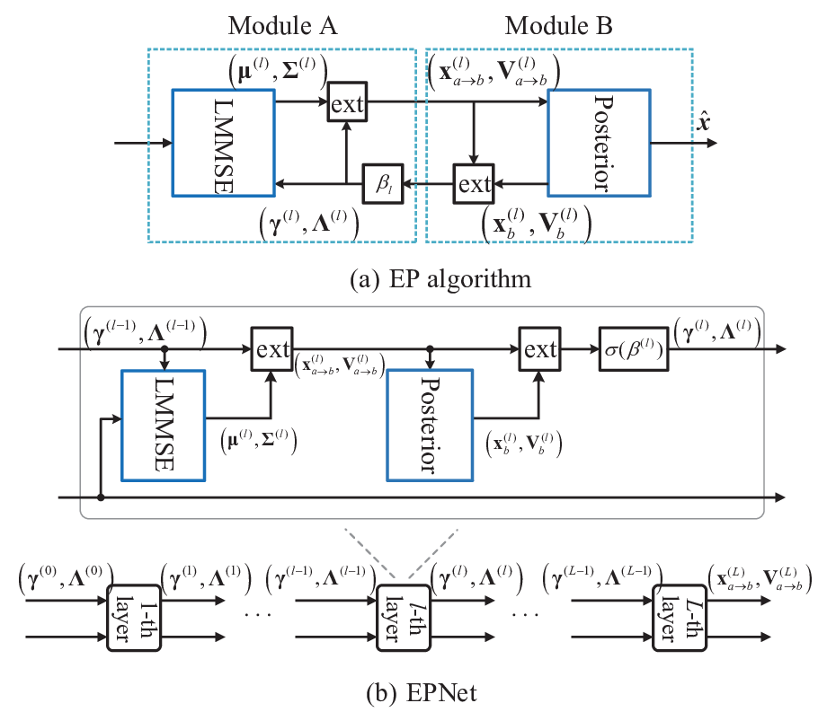
The diagram of EP is provided in Fig. 2(a), which shows the iteration between modules A and B. The passing of message from A to B is denoted as ${a\to b}$, and the reverse is denoted as ${b\to a}$. The pair $(\bm{\gamma},\bm{\Lambda})$ can be computed as follows:

• 1)

  The cavity marginal $q^{(l)\textbackslash n}(x_{n})={q^{(l)}(x_{n}|\bm{\gamma},\bm{\Lambda})}/{{{e}^{{{\gamma}_{n}}{{{{x}}}_{n}}-\frac{1}{2}{{\Lambda}_{n}}{x}_{n}^{2}}}}$ is computed.
  Given $q(\mathbf{{x}}|\bm{\gamma},\mathbf{\Lambda})\sim\mathcal{N}({\mathbf{x}};{{\bm{\mu}}^{(l)}},{{\bm{\Sigma}}^{(l)}})$, the extrinsic covariance matrix $\mathbf{{V}}_{a\to b}^{(l)}$ and the mean matrix $\mathbf{{x}}_{a\to b}^{(l)}$ of the cavity marginal can be derived as

  $$\left\{\begin{aligned} &\mathbf{{V}}_{a\to b}^{(l)}={{\left[{\left({{\bm{\Sigma}}^{(l)}}\right)^{-1}}-\mathbf{\Lambda}^{(l-1)}\right]}^{-1}},\\ &\mathbf{{x}}_{a\to b}^{(l)}=\mathbf{{V}}_{a\to b}^{(l)}\left[{\left({{\bm{\Sigma}}^{(l)}}\right)^{-1}}{{{\bm{\mu}}^{(l)}}}-\bm{\gamma}^{(l-1)}\right],\end{aligned}\right.$$

  (10)

• 2)

  The mean and variance of distribution $\hat{p}^{(l)}(x_{n}|\mathbf{y})\propto q^{(l)\textbackslash n}(x_{n}){p}_{\sf a}({{x}_{n}})$ are computed.
  The posterior mean matrix $\mathbf{{x}}_{b}^{(l)}$ and the covariance matrix $\mathbf{{V}}_{b}^{(l)}$ of $\hat{p}^{(l)}(\mathbf{x}|\mathbf{y})$ in module B are obtained from $\mathcal{N}({\mathbf{x}};\mathbf{{x}}_{a\to b}^{(l)},\mathbf{{V}}_{a\to b}^{(l)})$ and the real domain constellation, which can be expressed as

  $$\left\{\begin{aligned} &\mathbf{{V}}_{b}^{(l)}=\mathbb{V}{\left\{\mathbf{{x}}\big|\mathbf{{x}}_{a\to b}^{(l)},\mathbf{{V}}_{a\to b}^{(l)}\right\}},\\ &\mathbf{{x}}_{b}^{(l)}=\mathbb{E}{\left\{\mathbf{{x}}\big|\mathbf{{x}}_{a\to b}^{(l)},\mathbf{{V}}_{a\to b}^{(l)}\right\}},\end{aligned}\right.$$

  (11)

  where the expectations are derived from $\hat{p}^{(l)}(\mathbf{x}|\mathbf{y})$.

• 3)

  Pair $(\bm{\gamma}^{(l)},\bm{\Lambda}^{(l)})$ is refined with $\mathbb{E}_{q(\mathbf{x}|\mathbf{\Lambda},\bm{\gamma})}=\mathbb{E}_{\hat{p}(\mathbf{x}|\mathbf{y})}$ and $\mathbb{V}_{q(\mathbf{x}|\mathbf{\Lambda},\bm{\gamma})}=\mathbb{V}_{\hat{p}(\mathbf{x}|\mathbf{y})}$, and then is updated as

  $$\left\{\begin{aligned} &\mathbf{\Lambda}^{(l)}={\left(\mathbf{{V}}_{b}^{(l)}\right)}^{-1}-{\left(\mathbf{{V}}_{a\to b}^{(l)}\right)}^{-1},\\ &\bm{\gamma}^{(l)}={\left(\mathbf{{V}}_{b}^{(l)}\right)}^{-1}\mathbf{{x}}_{b}^{(l)}-{\left(\mathbf{{V}}_{a\to b}^{(l)}\right)}^{-1}\mathbf{{x}}_{a\to b}^{(l)}.\end{aligned}\right.$$

  (12)

Notably, $\bm{\Lambda}$ in (8) is an inverse variance term and should be positive. However, the parameter updated in (12) may return a negative value, resulting in the exploration of the numerical value and convergence failure. In such case, the previous values should be kept for those parameters [39]. In addition, parameter updating must be smoothed through a convex combination with the former value to improve the robustness of the algorithm [10]; that is,

Damping factors, $\bm{\beta}=[\beta^{(1)},...,\beta^{(L)}]$, are introduced to prevent the EP solution from exploding.

Updating $(\bm{\gamma}^{(l)},\bm{\Lambda}^{(l)})$ with a damping factor is crucial for maintaining the stability of the EP solution. However, convergence speed is affected by damping factors. We first review the parameter updating methods used in previous studies [11, 10, 13] and then explain those used in EPNet. In accordance with [10], several parameters, including minimum allowed variance $\epsilon$, damping procedure $\bm{\beta}$, and number of iterations $L$, must be tuned. $\epsilon$ ensures the non negativity of the variance, and $\bm{\beta}$ determines the stability and convergence speed of the algorithm. The computational complexity of the algorithm is linearly related to $L$. $\epsilon$ gradually decreases to avoid instability caused by fast updates. In [11], for example, when fast updates are performed (i.e., $\beta^{(l)}=0.95,\forall l\in\{1,\cdots,L\}$), $\epsilon$ started with a small value during the first four iterations and then exponentially decreased as $1/2^{\max(l-4,1)}$. However, the authors of [13] found that fast updates can induce instability for large modulations and turbo schemes. For the turbo receiver, the damping factors should be re-tuned in every turbo iteration [12, 13]. In [13], $\beta^{(l)}$ started with a conservative value and exponentially increased with the number of turbo iterations $i$, i.e., $\beta^{(l)}=\min(0.1\cdot e^{i/1.5},\,0.7)$. The growth of $\beta^{(l)}$ reduced the number of EP iterations when the turbo procedure was used. The parameter settings used in different methods are listed in Table I. Damping factors $\bm{\beta}$ are manually tuned in accordance with various scenarios to achieve a trade-off between convergence speed and stability. The tuning process of the damping factors is customized and exhibits low efficiency.

In contrast with the traditional EP, damping factors $\bm{\beta}$ are set as trainable parameters and trained by an unfolded NN, as shown in Fig. 2(b). Each layer in Fig. 2(b) contains one adjustable variable $\beta^{(l)}$. Therefore, the total number of learnable variables is equal to $L$ when $L$ layers are found. The convergence, stability, and speed of EP can be significantly improved through large data training by using the learnable damping factors. In contrast with other NN-based signal detectors, such as DetNet [17], the number of learnable variables of EPNet is independent of the number of antennas in MIMO systems and only related to the number of layers $L$. This characteristic is advantageous for large-scale MIMO systems. A sigmoid function, $\sigma(\cdot)$, is used to constrain the range of damping factors, i.e., $\sigma(\beta^{(l)})\in[0,1]$. Then, (13) is reformulated as

In JDD$-i$, the approximated extrinsic pdf $q_{\sf e}^{i}\sim\mathcal{N}({\mathbf{x}};\mathbf{{x}}_{a\to b}^{(L)},\mathbf{{V}}_{a\to b}^{(L)})$ is outputted by EPNet and demapped as extrinsic LLRs $L_{\sf e}^{i}$ in accordance with (4). Then, the extrinsic LLRs are delivered to TurboNet, outputting the new a priori LLRs $L_{\sf a}^{i}$. Subsequently, $L_{\sf a}^{i}$ is mapped as a priori pdf $p_{\sf a}^{i}$ to construct the mean and variance of constellation $(\tilde{\mathbf{x}}_{i},\widetilde{\mathbf{V}}_{i})$. In the JDD$-(i+1)$ phase, the initial pair of $(\bm{\gamma}^{(0)}_{i+1},\bm{\Lambda}^{(0)}_{i+1}),~i=1,\ldots,I-1$ for the corresponding EPNet is computed as

In JDD$-1$, the initiation is set as ${{\bm{\gamma}}^{(0)}_{1}}=\mathbf{0}$, ${{\mathbf{\Lambda}}^{(0)}_{1}}=\frac{1}{2{E}_{s}}\mathbf{I}_{2N_{t}}$.

In the JDD$-i$ of the unfolded turbo receiver, the initialization pair of $(\bm{\gamma}^{(0)}_{i},\bm{\Lambda}^{(0)}_{i})$ inputted into EPNet is more accurate than those inputted into the EPNet in JDD$-(i-1)$. Therefore, the EPNet in JDD$-i$ should readjust the damping factors. For the unfolded turbo receiver, EPNets are sequentially trained $I$ times. The total number of training parameters of EPNets for the unfolded turbo receiver is ${IL}$.

The number of training parameters of model-driven NN-based methods [22, 20, 23] significantly decreases compared with data-driven NN-based methods [40, 17]. In particular, EPNet can work in every channel realization with a baseline performance without training by using appropriate initial values of the damping factors, such as nonuniform block EP (nuBEP) in Table I. Training the damping factors can incrementally improve the baseline performance. However, these ${IL}$ trainable parameters of EPNets must be re-trained when the channel environment considerably changes. Consequently, an online training mechanism should be developed to adapt to environment changes.

In this subsection, an online training mechanism based on meta learning is introduced to learn the optimal damping factors of EPNets quickly.

In accordance with [41], an optimization algorithm based on meta learning can be modeled as a learning problem, which can be implemented using an LSTM network and replacing traditional optimization algorithms, such as Adam, root mean square prop (RMSprop), and stochastic gradient descent. The new optimizer outperforms these hand-designed optimization algorithms in terms of convergence speed and generalizes well to new tasks. Motivated by [41], an online training mechanism based on meta learning for EPNet is developed. In particular, we involve the training of two NNs. First, an LSTM optimizer is developed, as shown in Fig. 3. This optimizer is implemented using LSTM networks and can realize the function of gradient descent, similar to traditional optimizers. Second, EPNet is trained using the LSTM optimizer, and the optimizee is set as the damping factor and expected to reach convergence quickly.

Step 1: Learning the LSTM optimizer. The LSTM optimizer should be capable of learning the rules of gradient descent. To achieve this objective, an $L$-dimensional quadratic function is selected as the objective function of a task, such as the $j$-th task, which is expressed as

where $\mathbf{\mathbf{W}}_{j}$ is an $L\times L$ random matrix, and $\mathbf{\mathbf{q}}_{j}$ is an $L\times 1$ random vector. Each element of $\mathbf{\mathbf{W}}_{j}$ and $\mathbf{\mathbf{q}}_{j}$ follows standard normal distributions. $J$ denotes the number of tasks. Quadratic functions with $L$ dimensions are selected because EPNet is involved in $L$ layers. For different ${\mathbf{W}}_{j}$ and ${\mathbf{q}}_{j}$, the optimal $\bm{\beta}$ that achieves minimum $f({\bm{\beta}};{\mathbf{W}}_{j},{\mathbf{q}}_{j})$ varies. Therefore, different realizations of $\mathbf{\mathbf{W}}_{j}$ and ${\mathbf{q}}_{j}$ can constitute different tasks for meta learning.

A computational graph is used to compute the gradient of the optimizee, $\beta^{(l)}$, for the LSTM optimizer, as presented in Fig. 3. This figure shows an optimizee and an LSTM optimizer with $T$ time steps and $T$ LSTM units, where $t$ denotes the $t$-th time step of the LSTM optimizer; ${\cal G}$ denotes a LSTM unit with a specific number of hidden layer neurons and layers; $\beta_{t}^{(l)}$ is the $l$-th updated optimizee parameter in time step $t$; and $f_{t}$ denotes the value of (16) in the $t$-th time step, i.e., $f_{t}=f({\bm{\beta}}_{t};{\mathbf{W}}_{j},{\mathbf{q}}_{j})={\|{\mathbf{W}}_{j}{\bm{\beta}}_{t}-{\mathbf{q}}_{j}\|}^{2}$. In time step $t$, one input of ${\cal G}$ is the partial derivative, $\nabla_{t}^{(l)}$, which is computed as

The updating step of the optimizee, $g_{t}^{(l)}$, is the output of ${\cal G}$ in which its state is explicitly denoted by $h_{t-1}^{(l)}$. In general, the inputs of ${\cal G}$ in time step $t$ are $\nabla_{t-1}^{(l)}$ and ${h}_{t-1}^{(l)}$, and the outputs are ${g}_{t}^{(l)}$ and ${h}_{t}^{(l)}$. The updating rules for an LSTM unit and the optimizee are expressed as follows:

where ${\bm{\Theta}}$ represents all the adjustable parameters in LSTM unit ${\cal G}$ and is randomly initialized. The output of the LSTM optimizer is $g_{T}^{(l)}$, as shown in Fig. 3, which is the output of the LSTM unit ${\cal G}$ in the last time step. In particular, the gradients on ${\bm{\Theta}}$ are allowed to flow along solid lines, and the gradients along dashed lines are dropped. The arrows represent the passing of variables. Disregarding the gradients of ${\bm{\Theta}}$ along the dashed lines is tantamount to assuming that the gradient of the optimizee, ${\nabla}_{t}$, depends only on $f$ and exhibits no relationship with ${\bm{\Theta}}$, i.e., $\partial{{\nabla}_{t}}/\partial\Theta=0$ [41]. Therefore, the LSTM optimizer avoids calculating the second derivative of $f$, i.e., $\frac{{{\partial^{2}}f}}{{\partial\beta\partial\Theta}}$, reducing the complexity of training.

All the other optimizees $\bm{\beta}^{\textbackslash(l)}$ have the same computational graph as $\beta^{(l)}$ and use a structure identical to that in Fig. 3. However, the inputs and the hidden states are separate. The loss function for training the LSTM optimizer is computed as

The objective of training the LSTM optimizer is to minimize the value of $\mathcal{L}({\bm{\Theta}})$ by using the Adam optimizer on ${\bm{\Theta}}$, which is related to all the optimizees $\bm{\beta}$. During an epoch, $\beta^{(l)}$ is initialized as 1. Then, $\beta^{(l)}_{1}$ is updated $T$ time by the LSTM optimizer following (18), and obtains $\beta_{T}^{(l)}=\beta_{T-1}^{(l)}+g_{T}^{(l)}$. Lastly, $\bm{\beta}_{T}=[\beta_{T}^{(1)},\ldots,\beta_{T}^{(L)}]$ is inputted into (19), and ${\bm{\Theta}}$ is updated only once using the Adam optimizer by minimizing (19). In the succeeding epochs, we use $J$ new tasks, where ${\mathbf{W}}_{j}$ and ${\mathbf{q}}_{j}$ are regenerated, and $\bm{\beta}$ is reinitialized. The same process is repeated until the LSTM optimizer achieves convergence. After the LSTM optimizer reaches convergence, the updating step of the optimizee, $g_{t}^{(l)}$, is determined by the input of the LSTM unit ${\cal G}$,$\nabla_{t-1}^{(l)}$ and $h_{t-1}^{(l)}$. $g_{t}^{(l)}$ will be positive when $\nabla_{t-1}^{(l)}$ is negative, and $g_{t}^{(l)}$ will be negative when $\nabla_{t-1}^{(l)}$ is positive. Although $\nabla_{t}^{(l)}$ in (17) is only related to the current optimizee $\beta^{(l)}$ and unrelated to the other optimizees $\bm{\beta}^{\textbackslash(l)}$, $\mathbf{W}$ and $\mathbf{q}$ with $L$ dimensions are adopted. This setting is applied to improve the extensiveness of the trainable parameters ${\bm{\Theta}}$ of the LSTM optimizer and enables the trained LSTM optimizer to adjust to multiple optimizees in parallel. After training, the parameters of the LSTM unit, ${\bm{\Theta}}$, are obtained.

The LSTM optimizer can be used to update the optimizees in parallel during the testing phase because it is used to update different optimizees for various tasks during the training phase. In addition, the optimizer can be utilized to train other functions apart from quadratic functions, such as the loss function in EPNet. During the training of the LSTM optimizer, the dataset originated from the quadratic functions of (16). Although task (16) is nonidentical to that of EPNet, the LSTM optimizer can still provide better gradient descent than the traditional optimization algorithm for EPNet. This funding is attributed to the use of recurrence allowing the LSTM optimizer to learn dynamic updating rules that integrate information from the history of gradients, which is similar to momentum.

Step 2: Training the damping factors of EPNet by using the LSTM optimizer. The LSTM optimizer is utilized to train the damping factors of EPNet to achieve convergence quickly and increase the efficiency of online training. The loss on all the $L$ layers is defined as the loss function in training EPNet, which is expressed as follows⁴⁴ 4 The loss function is different from that in [24].:

The updating rule for $\bm{\beta}$ is determined by the LSTM optimizer, which has been trained in Step 1. The LSTM optimizer minimizes a new task $f_{\rm EP}(\bm{\beta})$ rather than (16).⁵⁵ 5 Note that $f$ in Fig. 3 is replaced by $f_{\rm EP}(\bm{\beta})$ in this step.

The online training mechanism begins to train the damping factors of EPNets when the channel condition considerably changes, such as the mobile terminal moving from indoor to outdoor. If the online training phase is triggered, then training labels $(\mathbf{x},\mathbf{y})$ are generated at the receiver side in accordance with (1), where the modulated symbols $\mathbf{x}$ are randomly generated given the transmitted constellation and the MIMO channel matrices $\mathbf{H}$ are based on those acquired during the previous period.⁶⁶ 6 Notice that the noise vector follows the standard Gaussian distribution since the channel matrices have been normalized. Subsequently, the damping factors of EPNets are trained by the LSTM optimizer by using the generated dataset. The damping factors for each EPNet are utilized online, enabling the unfolded turbo receiver to improve the performance of the traditional turbo receiver.

In the simulation, an ${8\times 8}$ or ${32\times 32}$ MIMO system is evaluated. The modulation is set to quadrature phase-shift keying (QPSK), 16-QAM, and 64-QAM. The channel matrix $\mathbf{H}$ is sampled from an independent and identical Gaussian distribution (i.e., each colume of $\mathbf{H}$ follows the distribution $\mathcal{N}_{\mathbb{C}}(0,(1/N_{r})\mathbf{I}_{N_{r}})$). For signal detection, the initiation parameters follow Table I for JDD. For channel decoding, the turbo code is used, where the message bit length $K$ is set to 40 or 120 and encoded using the convolutional encoder at a rate of $1/2$.

TurboNet and the LSTM optimizer are first trained off-line. Then, EPNets are trained by the LSTM optimizer online. TurboNet is trained by minimizing the cost [30, (16)] with the Adam optimizer at a learning rate of $10^{-5}$. The LSTM unit $\cal G$ is realized by two-layer LSTMs with five hidden units in each layer. time step $T$ is set to 20. The LSTM optimizer is trained by minimizing $\mathcal{L}$ in (19) with 20 tasks. Minimization is performed using Adam with a learning rate of $10^{-3}$. EPNet is trained by the LSTM optimizer with generated labels. Training data $(\mathbf{x,y})$ are generated by using (1) with $5,000$ channel realizations, and $f_{\rm EP}$ is selected as the cost function. The training parameters of TurboNet, the LSTM optimizer, and EPNet are summarized in Table II.

The following naming conventions are used to present the performance concisely, where EP and EPNet are outputs for an uncoded MIMO system and the others are outputs for turbo receivers (iteratively exchange LLRs between the signal detector and the channel decoder):

• •

  EP ($L=l$): EP with $l$ iterations, where the damping factor is set as 0.1 for each iteration.

• •

  EPNet ($L=l$): EPNet with $l$ layers, where the damping factors are trained by the LSTM optimizer.

• •

  EP+Turbo ($I=i$): EP for signal detection, and the max-log-MAP algorithm for channel decoding with $i$ iterations between the detector and the decoder.

• •

  EP+TurboNet ($I=i$): EP for signal detection, and TurboNet for channel decoding with $i$ iterations between the detector and decoder.

• •

  EPNet+Turbo ($I=i$): EPNet for signal detection, and the max-log-MAP algorithm for channel decoding with $i$ iterations between the detector and decoder.

• •

  EPNet+Turbo-log ($I=i$): EPNet for signal detection, and log-MAP algorithm for channel decoding with $i$ iterations between the detector and the decoder.

• •

  EPNet+TurboNet ($I=i$): EPNet for signal detection and TurboNet for channel decoding with $i$ iterations between the detector and the decoder.

We use $L=5$ and $I=4$ when no special illustrations are found.

The energy per bit to noise power ratios in the uncoded and coded systems are denoted as $E_{B}/N_{0}$ and $E_{b}/N_{0}$, respectively.⁷⁷ 7 For the MIMO system with $M$-QAM constellation, the relationship between $E_{b}/N_{0}$ and $E_{s}/N_{0}$ is expressed as $E_{s}/N_{0}=E_{b}/N_{0}+10\log\left(\log_{2}(M)\right)$. The relationship between $E_{B}/N_{0}$ and $E_{b}/N_{0}$ is expressed as $E_{B}/N_{0}=E_{b}/N_{0}+10\log(1/R)$. In this section, we assume that the received $E_{B}/N_{0}$ or $E_{b}/N_{0}$ in each antenna is identical to make the simulation results intuitive.

Table III presents the performance comparisons between EP and EPNet for ${8\times 8}$ uncoded MIMO systems with 16-QAM modulation. The performance of EPNet with 5 iterations is comparable with that of EP with 10 or 15 iterations. The computation complexity of EP and EPNet with 1 iteration is $\mathcal{O}(N_{t}^{3})$ [10]. Given the same computational complexity (e.g., $L=5$), the BER performance of the trainable EP (i.e., EPNet) can be immensely improved. We list the learned damping factors in Table III to improve the understanding of the characteristics of EPNet. At a low $E_{B}/N_{0}$ regime (e.g., $E_{B}/N_{0}$ $=-1$ and $4$ dB), the damping factors become extremely small after two iterations, implying that EPNet can reach convergence within two layers. Although EPNet requires many iterations to reach convergence at a high $E_{B}/N_{0}$ regime (e.g., $E_{B}/N_{0}$$=9$ and $14$ dB), it requires only four iterations. With the learned damping factors, we can determine the number of needed layers for EPNet, which is beneficial for reducing computational complexity. Notably, the damping factors vary with different $E_{B}/N_{0}$’s, indicating the importance of the online training mechanism because the environment constantly changes.

The convergence performance (loss versus epoch) of the online training mechanism is illustrated in Fig. 4. The loss value is the result of $f_{\rm EP}(\bm{\beta})$. The convergence speed of EPNet depends on the time steps in the LSTM optimizer. As shown in Fig. 4, the convergence speed of EPNet with 5 time steps is evidently slower than that of EPNet with 20 time steps. However, no considerable difference is observed with an increase in time steps (i.e., $T$=100). This phenomenon suggests that the LSTM optimizer can find the optimal damping factors in a specific epoch with limited time steps. Therefore, the time steps of the LTSM optimizer are set as 20 in the remaining part of this study. EPNet can also be optimized using traditional optimizers, such as Adam and RMSprop, with a learning rate of 0.1. Its convergence speed performance is shown in Fig. 4. Adam and RMSprop optimizers spend 80 and 90 epochs to reach convergence. By contrast, the LSTM optimizer reaches convergence within 20 epochs. The convergence speed of the LSTM optimizer is evidently faster than those of the other optimizers, suggesting the high capability of meta learning-based EPNet in adapting to new environments.

We compare existing detectors with the proposed EPNet. Jeon et al. [42] proposed an optimized AMP algorithm for MIMO detection, which runs 50 iterations to reach convergence in our simulation. For the Rayleigh channel, MMNet in the independent and identical distributed case [19, (11)] is adopted. When the channel is correlated, MMNet for arbitrary channel matrices [19, (13)] is used. The computation complexity of AMP and MMNet is both $L\mathcal{O}(N_{t}^{2})$. OAMPNet in [22], which is based on the OAMP algorithm [21], is implemented in five layers with two trainable parameters per layer. The computation complexity of the MMSE detector [37] is dominated by the matrix inversion in (9), which is $\mathcal{O}(N_{t}^{3})$. The OAMP, OAMPNet, EP and EPNet with $L$ iterations exhibits an $L$ matrix inversion operation, and thus, the computation complexity is $L\mathcal{O}(N_{t}^{3})$. ML with a complexity of $\mathcal{O}\left(|\mathcal{A}|^{N_{t}}\right)$ is an optimal baseline. The complexity comparison is concluded in Table IV. Fig. 5 presents the performance comparison among existing detectors with QPSK modulation. As shown in the figure, EPNet significantly outperform the existing algorithms either for the Rayleigh channel in $32\times 32$ MIMO systems or the 3GPP 3D correlated channel [19] in $64\times 32$ MIMO systems. In addition, EPNet with five iterations can nearly achieve the performance of ML for the Rayleigh channel.

Fig. 6 shows the performance comparison among different turbo decoding algorithms, including max-log-MAP, log-MAP, and TurboNet, for QPSK, 16-QAM, and 64-QAM modulations. The computational complexity of TurboNet is comparable with the max-log-MAP algorithm but lower than the log-MAP algorithm. In Fig. 6, $(K,R)$ indicates that $K$ message bits are encoded by the turbo encoder at an $R$ rate. As shown in Fig. 6, the performance of TurboNet is better than that of the max-log-MAP and comparable with that of the log-MAP algorithm. The results indicate that TurboNet can achieve better BER performance or lower computational complexity than the competing decoding algorithms. For $(40,1/2)$, performance improvement can be easily observed for QPSK at 16-QAM. However, improvement is inevident for 64-QAM because the code length is extremely short for high-order modulation. The improvement of TurboNet for 64-QAM becomes more evident compared with that of the max-log-MAP algorithm when code length increases (i.e., message bit length is 120). In particular, TurboNet is trained in AWGN channels with binary phase-shift keying modulation and low $E_{b}/N_{0}$ but is applied to Rayleigh fading channels with high-order modulation and high $E_{b}/N_{0}$, indicating the robustness of TurboNet. Consequently, TurboNet is trained off-line only once because of this characteristic.

References

- [1] Y. S. Cho, J. Kim, W. Y. Yang, and C. G. Kang, MIMO-OFDM Wireless Communications with MATLAB. John Wiley and Sons, 2010.
- [2] C.-Y. Tsai, K.-L. Wong, and W.-Y. Li, “Experimental results of the multi-Gbps smartphone with 20 MIMO antennas in the 2012 MIMO operation,” Microwave Opt. Technol. Lett., vol. 60, pp. 2001–2010, Aug. 2018.
- [3] A. Zhao and Z. Ren, “Size reduction of self-isolated MIMO antenna system for 5G mobile phone applications,” IEEE Antennas Wirel. Propag. Lett., vol. 18, no. 1, pp. 152–156, Jan 2019.
- [4] V. Raghavan and J. Li, “Evolution of physical-layer communications research in the post-5G era,” IEEE Access, vol. 7, pp. 10 392–10 401, Jan. 2019.
- [5] S. Yang and L. Hanzo, “Fifty years of mimo detection: The road to large-scale mimos,” IEEE Commun. Surveys Tuts., vol. 17, no. 4, pp. 1941–1988, Fourthquarter 2015.
- [6] D. L. Donoho, A. Maleki, and A. Montanari, “Message passing algorithms for compressed sensing,” Proc. Nat. Acad. Sci., vol. 106, no. 45, pp. 18 914–18 919, Nov. 2009.
- [7] T. P. Minka, A FAMILY OF ALGORITHMS FOR APPROXIMATE BAYESIAN INFERENCE. Ph.D. dissertation, Dept. Elect. Eng. Comput. Sci., MIT, Cambridge, MA, USA, 2001.
- [8] S. Wu, L. Kuang, Z. Ni, J. Lu, D. Huang, and Q. Guo, “Low-complexity iterative detection for large-scale multiuser MIMO-OFDM systems using approximate message passing,” IEEE J. Sel. Topics Signal Process., vol. 8, no. 5, pp. 902–915, Oct 2014.
- [9] M. W. Seeger, Expectation Propagation For Exponential Families. Univ. Calif., Berkeley, CA, USA, Tech. Rep., 2005.
- [10] J. Céspedes, P. M. Olmos, M. Sánchez-Fernández, and F. Perez-Cruz, “Expectation propagation detection for high-order high-dimensional MIMO systems,” IEEE Trans. Commun., vol. 62, no. 8, pp. 2840–2849, Aug. 2014.
- [11] ——, “Probabilistic MIMO symbol detection with expectation consistency approximate inference,” IEEE Trans. Veh. Technol., vol. 67, no. 4, pp. 3481–3494, Apr. 2018.
- [12] I. Santos, J. J. Murillo-Fuentes, E. A. de Reyna, and P. Olmos, “Turbo EP-based equalization: a filter-type implementation,” IEEE Trans. Commun., vol. 66, no. 9, pp. 4259–4270, Sep. 2017.
- [13] I. Santos and J. J. Murillo-Fuentes, “EP-based turbo detection for MIMO receivers and large-scale systems,” 2018. [Online]. Available: https://arxiv.org/abs/1805.05065
- [14] I. Santos, J. J. Murillo-Fuentes, and E. Arias-de-Reyna, “A double EP-based proposal for turbo equalization,” IEEE Signal Process. Lett., vol. 27, pp. 121–125, Dec. 2019.
- [15] H. He, S. Jin, C.-K. Wen, F. Gao, G. Y. Li, and Z. Xu, “Model-driven deep learning for physical layer communications,” IEEE Wireless Commun., vol. 26, no. 5, pp. 77–83, Oct. 2019.
- [16] A. Balatsoukas-Stimming and C. Studer, “Deep unfolding for communications systems: A survey and some new directions,” in Proc. IEEE International Workshop on Signal Processing Systems (SiPS), Nanjing, China, Oct. 2019, pp. 266-271.
- [17] N. Samuel, T. Diskin, and A. Wiesel, “Learning to detect,” IEEE Trans. Signal Process., vol. 67, no. 10, pp. 2554–2564, May 2019.
- [18] X. Jin and H. Kim, “Parallel deep learning detection network in the MIMO channel,” IEEE Commun. Lett., vol. 24, no. 1, pp. 1–4, Oct. 2019.
- [19] M. Khani, M. Alizadeh, J. Hoydis, and P. Fleming, “Adaptive neural signal detection for massive MIMO,” IEEE Trans. Wireless Communi., Early Access, 2020.
- [20] D. Ito, S. Takabe, and T. Wadayama, “Trainable ISTA for sparse signal recovery,” IEEE Trans. Signal Process., vol. 67, no. 12, pp. 3113–3125, Jun. 2019.
- [21] J. Ma and L. Ping, “Orthogonal AMP,” IEEE Access, vol. 5, no. 14, pp. 2020–2033, Jan. 2017.
- [22] H. He, C.-K. Wen, S. Jin, and G. Y. Li, “Model-Driven Deep Learning for MIMO Detection,” IEEE Trans. Signal Process., vol. 68, pp. 1702-1715, Feb. 2020.
- [23] J. Zhang, H. He, C.-K. Wen, S. Jin, and G. Y. Li, “Deep learning based on orthogonal approximate message passing for CP-free OFDM,” in Proc. IEEE International Conference on Acoustics, Speech and Signal Processing (ICASSP), Brighton, UK, May 2019, pp. 1–6.
- [24] S. Sahin, C. Poulliat, A. M. Cipriano, and M. Boucheret, “Doubly iterative turbo equalization: Optimization through deep unfolding,” in Proc. IEEE Annual International Symposium on Personal, Indoor and Mobile Radio Communications (PIMRC), Istanbul, Turkey, Sep. 2019, pp. 1–6.
- [25] P. Jiang, T. Wang, B. Han, X. Gao, J. Zhang, C.-K. Wen, S. Jin, and G. Y. Li, “Artificial intelligence-aided OFDM receiver: Design and experimental results,” 2018. [Online]. Available: https://arxiv.org/abs/1812.06638
- [26] N. Shlezinger, N. Farsad, Y. C. Eldar, and A. J. Goldsmith, “Viterbinet: A deep learning based viterbi algorithm for symbol detection,” IEEE Trans. Wireless Commun., vol. 19, no. 5, pp. 3319-3331, May 2020.
- [27] V. Ricardo and D. Youssef, “A perspective view and survey of meta-learning,” Artificial Intelligence Review, vol. 18, Sep. 2001.
- [28] H. Wu, Z. Zhang, C. Jiao, C. Li, and T. Q. S. Quek, “Learn to sense: a meta-learning based sensing and fusion framework for wireless sensor networks,” IEEE Internet of Things J., vol. 6, no. 5, pp. 8215-8227, Oct. 2019.
- [29] S. Park, H. Jang, O. Simeone, and J. Kang, “Learning to demodulate from few pilots via off-line and online meta-learning,” in Proc. IEEE International Workshop on Signal Processing Advances in Wireless Communications (SPAWC), Cannes, France, Jul. 2019, pp. 1-5.
- [30] Y. He, J. Zhang, C.-K. Wen, and S. Jin, “Turbonet: A model-driven dnn decoder based on max-log-map algorithm for turbo code,” in Proc. IEEE VTS Asia Pacific Wireless Communications Symposium (APWCS), Singapore, Aug. 2019, pp. 1–5.
- [31] D. P. Kingma and J. Ba, “Adam: A method for stochastic optimization,” 2014. [Online]. Available: https://arxiv.org/abs/1412.6980
- [32] 3rd Generation Partnership Project; Technical Specification; Evolved Universal Terrestrial Radio Access (E-UTRA); Multiplexing and Channel Coding (Release 9) 3GPP Organizational Partners TS 36.212, Rev. 8.3.0, May 2008.
- [33] J. Erfanian, S. Pasupathy, and G. Gulak, “Reduced complexity symbol detectors with parallel structure for ISI channels,” IEEE Trans. Commun., vol. 42, no. 234, pp. 1661–1671, Feb. 1994.
- [34] C. Berrou, A. Glavieux, and P. Thitimajshima, “Near shannon limit error-correcting coding and decoding: Turbo-codes,” in Proc. IEEE International Conference on Communications (ICC), Geneva, Switzerland, May 1993.
- [35] P. Robertson, P. Hoeher, and E. Villebrun, “Optimal and sub-optimal maximum a posteriori algorithms suitable for turbo decoding,” Eur. Trans. Telecommun., vol. 8, no. 2, pp. 119–125, Mar. 1997.
- [36] M. J. Wainwright and M. I. Jordan, “Graphical models, exponential families, and variational inference,” Found. Trends Mach. Learn., vol. 1, no. 1/2, Nov. 2008.
- [37] G. Caire, R. R. Muller, and T. Tanaka, “Iterative multiuser joint decoding: optimal power allocation and low-complexity implementation,” IEEE Trans. Inf. Theory, vol. 50, no. 9, pp. 1950–1973, Sep. 2004.
- [38] C. E. Rasmussen and C. K. I. Williams, Gaussian processes for machine learning. MIT Press, 2006.
- [39] J. Céspedes, APPROXIMATE INFERENCE IN MASSIVE MIMO SCENARIOS WITH MOMENT MATCHING TECHNIQUES. Ph.D. dissertation, Universidad Carlos III de Madrid, Jan. 2017.
- [40] H. Ye, G. Y. Li, and B. H. Juang, “Power of deep learning for channel estimation and signal detection in OFDM systems,” IEEE Wireless Commun. Lett., vol. 7, no. 1, pp. 114–117, Feb. 2018.
- [41] M. Andrychowicz, M. Denil, S. Gomez, M. W. Hoffman, D. Pfau, T. Schaul, B. Shillingford, and N. de Freitas, “Learning to learn by gradient descent by gradient descent,” in Proc. Neural Information Processing Systems (NIPS), Barcelona, Spain, Dec. 2016, pp. 1–6.
- [42] C. Jeon, R. Ghods, A. Maleki, and C. Studer, “Optimality of large mimo detection via approximate message passing,” in Proc. IEEE International Symposium on Information Theory (ISIT), 2015, pp. 1227–1231.
- [43] W. Tang, H. Prabhu, L. Liu, V. Owall, and Z. Zhang, “A 1.8Gb/s 70.6pJ/b 12816 link-adaptive near-optimal massive MIMO detector in 28nm UTBB-FDSOI,” in Proc. IEEE International Solid-State Circuits Conference (ISSCC), 2018, pp. 224–226.