Detection power of separability criteria based on a correlation tensor: a case study

Quantum entanglement defines a key feature of quantum theory. It becomes a crucial resource for quantum information theory and for modern quantum based technologies like quantum communication, quantum cryptography, and quantum calculations HHHH; QIT. There are several separability criteria developed during the last two decades which enable to distinguish between separable and entangled states (cf. GT; HHHH; TOPICAL). In this paper we analyze a special family of separability criteria based on correlation tensor. The prominent example is provided be the realignment criterion or computable cross-norm (CCNR) criterion R1; R2; R3. Apart from CCNR this class contains de Vicente criterion (dV) Vicente, separability criterion derived in Fei and recent criterion based on SIC POMVs (ESIC) GUHNE. Interestingly, all these criteria were unified in GGD1. It was shown GGD1 that the above criteria are just special examples of a 2-parameter family of criteria. In this paper we provide a comparative anaysis of these criteria testing a simple family of bipartite states in $d_{1}\otimes d_{2}$.

Let us fix notation: $\mathbb{C}^{\mathrm{d_{1}}}\otimes\mathbb{C}^{\mathrm{d_{2}}}$ be the Hilbert space of a bipartite system with dimension of subsystems $d_{1}$ and $d_{2}$ respectively. In what follows we assume that $d_{2}\geq d_{1}$. Let $\{G_{\alpha}^{(1)}\}_{\alpha=1}^{d_{1}}$ and $\{G_{\beta}^{(2)}\}_{\beta=1}^{d_{2}}$ be arbitrary orthonormal bases in $\mathcal{B}(\mathbb{C}^{\mathrm{d_{1}}})$ and $\mathcal{B}(\mathbb{C}^{\mathrm{d_{2}}})$, namely $\langle G_{\alpha}^{(1)}|G_{\alpha^{\prime}}^{(1)}\rangle_{{\rm HS}}=\delta_{\alpha,\alpha^{\prime}}$ and the same for $G_{\beta}^{(2)}$, where $\langle X|Y\rangle_{\mathrm{HS}}={\rm Tr(X^{\dagger}Y)}$ is the Hilbert-Schmidt inner product. One defines a correlation matrix

Let us now restrict ourselves to orthonormal bases (referred as canonical bases) such that $G^{(i)}_{0}=\boldsymbol{1}_{\mathrm{d_{i}}}/\sqrt{d_{i}}$ (the remaining basis elements are then pairwise orthogonal hermitian traceless operators of norm one). Since now $C^{\mathrm{can}}$ stands for the correlation matrix in canonical bases. One proves GGD1) the following

Interestingly, for $(x,y)=(1,1)$ the above criterion reduces to CCNR. Moreover, for $(x,y)=(0,0)$, $(x,y)=\sqrt{2/d_{1}},\sqrt{2/d_{2}})$, and $(x,y)=(\sqrt{d_{1}+1},\sqrt{d_{2}+1})$ one recovers separability criteria developed in Vicente, Fei and GUHNE, respectively. The last criterion GUHNE was constructed in terms of SIC POMVs (ESIC criterion) and it was conjectured that it is stronger than original CCNR criterion. In this paper we provide a comparative analysis of CCNR, ESIC and dV criteria for a class of bipartite states being a generalization of well known isotropic states

where $|\psi^{+}_{d_{1}}\rangle=1/\sqrt{d_{1}}\sum_{i=1}^{d_{1}}|e_{i}\otimes f_{i}\rangle$, $|e_{i}\rangle$ defines orthonormal basis in $\mathbb{C}^{d_{1}}$ and $|f_{i}\rangle$ defines orthonormal set in $\mathbb{C}^{d_{2}}$. It is well known GT that this state is separable if and only if it is PPT which is equivalent to

In the paper we provide the upper bound for ‘$p$’ implied by condition (2). Moreover, we show that ESIC criterion detects more entangled state than the standard CNNR criterion. This supports the conjecture made in GUHNE that ESIC is stronger than CCNR. Finally, we analyze so called enhanced realignment criterion ZZZ which states that for separable states

with $\rho_{A}={\rm Tr}_{B}\rho_{AB}$ and $\rho_{B}={\rm Tr}_{A}\rho_{AB}$ being marginal states. Enhanced realignment criterion turns out to be the strongest effectively computable simplification of Correlation Matrix CriterionCOV-1; COV-2; COV-3 (see also COV-U for the unifying approach). In the recent papers GGD2 we showed that this criterion is equivalent to (2) for all $x,y\geq 0$. Here we show intricate relation of (7) and (2) using a family of isotropic states.

The main result of our paper consists in the following

For the proof cf. Appendix. Note, that for $x=y$ and $d_{1}=d_{2}=d$ one finds

and hence one recovers the PPT condition (6). In general, however,

and hence this criterion is weaker than PPT condition. In particular, we have the following bounds for de Vicente criterion ($x=y=0$), realignment criterion $x=y=1$, and for ESIC criterion ($x=\sqrt{d_{1}+1}$, $y=\sqrt{d_{2}+1}$):

We skip the expression $p_{F}$ for the criterion from Fei ($x=\sqrt{2/d_{1}}$,$y=\sqrt{2/d_{2}}$) since it is quite complicated. Again, for $d_{1}=d_{2}$ one has

For the proof cf. Appendix.

Separability of $\rho_{p}$ implies $p\leq p_{xy}$. Clearly, $p_{xy}$ depends on $(x,y)$ and hence the most efficient criterion corresponds to minimal value of $p_{xy}$. Let us calculate the minimum of the expression (8). One has

This is a necessary condition for minimum. One can check, that substituting (16) to (8) a constant value $\Gamma/\sqrt{1+\gamma}$ is obtained, hence we have the whole line $(1+\gamma)\tilde{y}=\tilde{x}-\gamma$ (hyperbola in $x$,$y$) of minima of $p_{xy}$. One can summarise the above observations in the following

The enhanced realignment criterion states that if $\rho_{p}$ is separable, then

where

are local states in the subsystems.

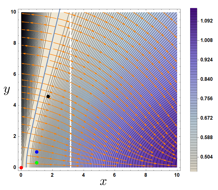
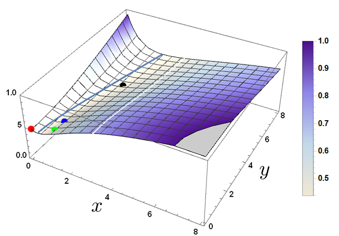
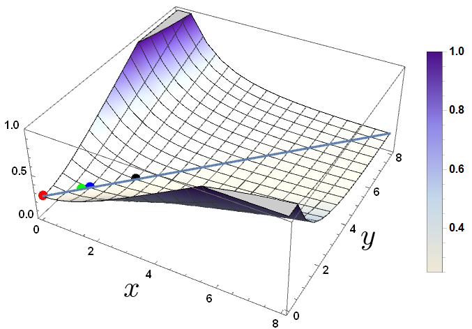
For the proof cf. Appendix. Hence, the enhanced realignment criterion is equivalent to the to the family of $XY$-criteria minimising $p_{xy}$. Interestingly, in GGD2 we proved that this equivalence is always realized for large values of $x$ and $y$, but for isotropic states in Eq. (5) it is enough consider $x,y$ belonging to the hyperbola in Eq. (17). Indeed, the figure 1 illustrates the hyperbola of minima of $p_{xy}$ (reducing to line if dimensions are equal) and four characteristic points representing the four criteria distinguished in the literature.

We provided a comparative analysis of the detection power of a $XY$-family of separability criteria in the case of generalized isotropic state in $d_{1}\otimes d_{2}$. Due to the high symmetry of the isotropic state one can derive analytical formula for the separability bound $p_{xy}$ which for $d_{1}\neq d_{2}$ is always higher than a PPT bound $p_{\mathrm{PPT}}=1/(d_{2}+1)$. Interestingly, minimising over $(x,y)$ we showed that the most efficient $p_{\rm min}$ is exactly the same as the one derived in term of so called enhanced realignment criterion. Finally, it is shown that for a family of generalized isotropic states the ESIC criterion from GUHNE detects more entangled state than original CCNR criterion. Hence, it supports a conjecture raised in GUHNE that ESIC is stronger than CCNR. It is clear that a similar analysis can be performed for a Werner-like state Werner

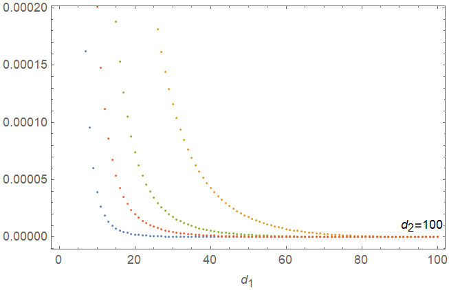
As a resume of this simple analysis, which provides a clear illustration of the detection power for a family of separability criteria based on correlation tensor, on figure is shown the general trend for large value of $d_{1}$ and $d_{2}$.

References

• [1] R. Horodecki, P. Horodecki, M. Horodecki, and K. Horodecki, Rev. Mod. Phys. 81, 865 (2009).
• [2] M. A. Nielsen and I. L. Chuang, Quantum Computation and Quantum Information (Cambridge University Press, Cambridge, England, 2000).
• [3] O. Gühne and G. Tóth, Phys. Rep. 474, 1 (2009).
• [4] D. Chruściński and G. Sarbicki, J. Phys. A: Math. Theor. 47, 483001 (2014).
• [5] K. Chen and L.-A. Wu, Quantum Inf. Comput. 3, 193 (2003).
• [6] K. Chen and L.-A. Wu, Phys. Rev. A 69, 022312 (2004).
• [7] O. Rudolph, Quantum Inf. Proccess. 4, 219 (2005).
• [8] J. D. Vicente, Quant. Inf. Comput. 7, 624 (2007).
• [9] M. Li, J. Wang, S.-M. Fei, and X. Li-Jost, Phys. Rev. A 89, 022325 (2014).
• [10] J. Shang, A. Asadian, H. Zhu, and O. Gühne, Phys. Rev. A 98, 022309 (2018).
• [11] G. Sarbicki, G. Scala, and D. Chruściński, Phys. Rev. A 101, 012341 (2020).
• [12] G. Sarbicki, G. Scala, and D. Chruściński, J. Phys. A: Math. Ther. 53, 455302 (2020).
• [13] C.-J. Zhang, Y.-S. Zhang, S. Zhang, and G.-C. Guo, Phys. Rev. A 77, 060301(R) (2208).
• [14] O. Gühne, P. Hyllus, O. Gittsovich, and J. Eisert, Phys. Rev. Lett. 99, 130504 (2007).
• [15] O. Gittsovich and O. Gühne, Phys. Rev. A 81 2010.
• [16] M. Li, S.-M. Fei, and Z.-X. Wang, J. Phys. A: Math. Theor. 41, 202002 (2008).
• [17] O. Gittsovich and O. Gühne, Phys. Rev. A 81, 032333 (2010).
• [18] J. Watrous, The Theory of Quantum Information, (Cambridge University Press, 2018)
• [19] A. Gilchrist, D. R. Terno, C. J. Wood, Vectorization of quantum operations and its use, arXiv:0911.2539v2
• [20] R.F. Werner, Phys. Rev. A 40, 4277 (1989).