Nearest Centroid Classification on a Trapped Ion Quantum Computer

Sonika Johri Affiliation: IonQ Inc, 4505 Campus Dr, College Park, MD 20740 Shantanu Debnath Affiliation: IonQ Inc, 4505 Campus Dr, College Park, MD 20740 Avinash Mocherla Affiliation: QC Ware, Palo Alto, USA and Paris, France Affiliation: UCL, Centre for Nanotechnology, London, UK Alexandros Singh Affiliation: QC Ware, Palo Alto, USA and Paris, France Affiliation: Université Sorbonne Paris Nord, France Anupam Prakash Affiliation: QC Ware, Palo Alto, USA and Paris, France Jungsang Kim Affiliation: IonQ Inc, 4505 Campus Dr, College Park, MD 20740 Iordanis Kerenidis Affiliation: QC Ware, Palo Alto, USA and Paris, France Affiliation: CNRS, University of Paris, France

Abstract

Quantum machine learning has seen considerable theoretical and practical developments in recent years and has become a promising area for finding real world applications of quantum computers. In pursuit of this goal, here we combine state-of-the-art algorithms and quantum hardware to provide an experimental demonstration of a quantum machine learning application with provable guarantees for its performance and efficiency. In particular, we design a quantum Nearest Centroid classifier, using techniques for efficiently loading classical data into quantum states and performing distance estimations, and experimentally demonstrate it on a 11-qubit trapped-ion quantum machine, matching the accuracy of classical nearest centroid classifiers for the MNIST handwritten digits dataset and achieving up to $100\%$ accuracy for 8-dimensional synthetic data.

I Introduction

Quantum technologies promise to revolutionize the future of information and communication, in the form of quantum computing devices able to communicate and process massive amounts of data both efficiently and securely using quantum resources. Tremendous progress is continuously being made both technologically and theoretically in the pursuit of this long-term vision.

A primary goal of current quantum computing research is to find real-world applications of the quantum computers that will become available in the coming years. In order to arrive at these first applications, simultaneous progress on both hardware and algorithms is required.

On the one hand, quantum hardware is making considerable advances. Small quantum computers capable of running representative algorithms were first made available in research laboratories, utilizing both trapped ion DebnathNature2016; MonzScience2016 and superconducting qubits BarendsNature2014; CorcolesNatCom2015. Performance comparisons among different quantum computer hardware have been made for running a host of quantum computing tasks LinkePNAS2017; MuraliISCA2019. Access to noisy intermediate-scale quantum (NISQ) computers from several commercial vendors is now available through cloud services. A recent report on achieving quantum supremacy, where a task was performed by a quantum computer that cannot be simulated with any available classical computer AruteNature2019, is an indication that powerful quantum computers will likely be available to researchers in the near future.

At the same time, considerable algorithmic work is underway in order to reduce the resources needed for implementing impactful quantum algorithms and bring them closer to the NISQ era. For example, more NISQ variants of amplitude estimation algorithms, a fundamental quantum procedure that is used in a large number of quantum algorithms, appeared recently suzuki2020amplitude; tanaka2020amplitude; grinko2019iterative; aaronson2020quantum; qfin2020. Another example are compilation techniques for optimizing the number of quantum gates that have resulted in a reduction in the number of qubits and gates for the factoring algorithm by many orders of magnitude gidney2019factor.

In this work, we focus on the area of quantum machine learning. There are a number of reasons why machine learning is a good area for trying to find applications of quantum computers. First, classical machine learning has proved to be an extremely powerful tool for a plethora of sectors, including Healthcare, Automotive, Manufacturing and Finance, so understanding the enhancements quantum computing can offer to this area will have a major impact. Second, we already know that fault-tolerant quantum computers with fast quantum access to classical data can provably offer advantages for many different applications such as classification, clustering and recommendation systems lloyd2014quantum; kerenidis2016quantum; kerenidis2019qmeans; li2019sublinear. In this work, we will show that there are concrete avenues for reducing the resources needed for implementing some core elements of such algorithms, in particular for loading classical data as quantum states and performing distance estimation between data points. Another interesting point is that it is desirable for classical machine learning algorithms to be robust against noise inherent in the data. To this end, regularization techniques that artificially inject noise into the computation are often used to improve generalization performance for classical neural networks noiseNN2017. Thus, one might hope that noisy quantum computers are inherently better suited for machine learning computations than for other types of problems that need precise computations like factoring or search problems. Last, there are many performance measures one may want to improve when it comes to machine learning - in addition to efficiency and accuracy, metrics like interpretability, transparency, and energy consumption are important ones where quantum computing may offer an advantage.

However, there are significant challenges to be overcome to make quantum machine learning practical. First, most quantum machine learning algorithms that offer considerable speedups assume that there are efficient ways to load classical data into quantum states. We address this bottleneck in this paper and describe ways to load a classical data point with logarithmic depth quantum circuits and using a number of qubits equal to the features of the data point. Another algorithmic bottleneck is that the solution output by the algorithm is oftentimes a quantum state from which one needs to extract some useful classical information. At times this can be efficient, for example, when an estimate on the distance between two such states or the identification of heavy-hitters is desired. In general, an exponential amount of time may be needed to extract the classical description of the quantum state by performing tomography.

One also needs to be careful with the efficiency of many of the quantum subroutines used in quantum machine learning, in particular linear algebra subroutines, since their running time depends on a large number of instance-specific parameters that need to be taken into account before claiming any speedups. In particular, most of these speedups will be polynomial and not exponential, and this is also corroborated by quantum inspired algorithms tang2019quantum. In any case, we believe the right way to describe these quantum speedups may not be to merely state them as exponential or polynomial, but to quantify the extent of speedup for each application and to see how these theoretical speedups translate in practice.

Another promising avenue for quantum machine learning pertains to the use of parametrized quantum circuits as analogues of neural networks for supervised learning, in particular for classification QNN2018; CNN2019. In fact, classical neural networks achieve extremely high performance for specific classification tasks like image classification, and one hopes that quantum analogues can achieve speedups and further enhance the accuracy of such techniques. Again, one needs to be careful, since we neither have much theoretical evidence that such quantum architectures will be easily trained, nor can we perform large enough simulations to get any convincing practical evidence of their performance (since we do not have large enough quantum hardware and classical simulations incur an exponential overhead). For example, architectures that use only a constant depth and only gates between consecutive qubits, while being suitable for near-term quantum computers, cannot really act as a fully connected neural network, since each input qubit can only affect a constant number of output qubits. It is also becoming clear that the time to train such quantum variational circuits can be quite large, both because of phenomena such as barren plateaus and also since designing the architectures, choosing cost-functions and initializing the parameters is far more complex and subtle than one may naively think QCNNplateaus2020; VQCA2020; Train2020. Further work is needed to understand the power and limitations of variational quantum circuits for machine learning applications.

Our work is a collaboration between quantum hardware and software teams that advances the state-of-the-art of quantum machine learning implementations, bringing potential applications closer to reality. Even though the scale of the implementation remains a proof of concept, our work makes significant progress towards unblocking a number of theoretical and practical bottlenecks. In particular, we look at classification, one of the canonical problems in supervised learning with a vast number of applications. In classification, one uses a labelled dataset (for example, emails labelled as Spam or Not Spam) to fit a model which is then used to predict the labels for new data points (for example, predict whether a new email should be labelled Spam or Not Spam). There are many different ways to perform classification that one can broadly place in two main categories.

The first way is similarity-based learning, where a notion of similarity between data points is defined (e.g. the Euclidean distance between data points seen as vectors) and points are classified together if they are similar. Well-known similarity-based algorithms are the Nearest Centroid, $k$ -Nearest Neighbors, Support Vector Machines, etc. The second way is based on deep learning techniques, in particular on different types of neural networks (fully connected, convolutional, recurrent, etc.). Here, the corpus of labelled data is used in order to train the weights of a neural network so that once trained it can infer the label of new data. Often, especially in cases where there is a large amount of data, neural networks can achieve better performance than more traditional similarity-based methods. On the other hand, similarity-based methods can offer other advantages, including provable performance guarantees and also properties like interpretability and transparency, which are becoming increasingly important in many sectors with sensitive data and decision making.

Here, we focus on demonstrating a quantum analogue of the Nearest Centroid algorithm, a simple similarity-based classification technique. The Nearest Centroid algorithm is a good baseline classifier that offers interpretable results, nevertheless, its performance deteriorates when the data points are far away from belonging to convex classes with similar variances. The algorithm takes as input a number of labelled data points, where each data point belongs to a specific class. The model fitting part of the algorithm is very simple and it involves computing the centroids, i.e. the barycenters of each of the sets. Once the centroids of each class are found, then a new data point is classified by finding the centroid which is nearest to it in Euclidean distance and assigning the corresponding label.

In our work, we design a quantum Nearest Centroid algorithm, by constructing quantum procedures for loading the classical data as quantum states and performing a distance estimation procedure. We demonstrate the quantum Nearest Centroid algorithm on up to 8 qubits of a trapped ion quantum processor and achieve accuracies comparable to corresponding classical classifiers on real datasets, as well as 100% accuracies on synthetic data. To our knowledge, this is the largest and most accurate classification demonstration on quantum computers. Importantly, we develop an error mitigation technique and noise model analysis that prove this performance will continue to hold as the problem size scales up.

Related experimental work. We describe here some previous work on classification experiments on quantum computers, in particular with neural networks. In fact, there is a fast growing literature on variational methods for classification on small quantum computers QNN2018; CNN2019; Image2020; Semisupervised2020; Polyadic2020; Dressed2020; Supervised2018; Hierarchical2018 of which we briefly describe those that also include hardware implementations. In Supervised2018, the authors provide binary classification methods based on variational quantum circuits. The classical data is mapped into quantum states through a fixed unitary transformation and the classifier is a short variational quantum circuit that is learned through stochastic gradient descent. A number of results on synthetic data are presented showing the relation of the method to Support Vector Machines classification and promising performance for such small input sizes. In Hierarchical2018 the authors provide a number of different classification methods, based on encoding the classical data in separable qubits and performing different quantum circuits as classifiers, inspired by Tree Tensor Network (TTN) and Multi-Scale Entanglement Renormalization Ansatz (MERA) circuits. A 4-qubit hardware experiment for a binary classification task between two of the IRIS dataset classes was performed on an IBM machine with high accuracy. In Polyadic2020, the authors performed 2-qubit experiments on IBM machines and with the IRIS dataset. They reported high accuracy for a subset of the dataset after training a quantum variational circuit for more than an hour and 3 million circuit runs.

The remainder of the paper is organized as follow: Section II explains the algorithm and software development. The experimental results and noise model are described in Section III. We end with a discussion in Section IV.

II Algorithm and Software

In this section, we describe the algorithm and software tools we used to implement quantum classification.

II.1 Data loaders and distance estimation

We start by describing our data loaders Ker2020. Being able to load classical data as quantum states that can be efficiently used for further computation is an important step for machine learning applications, since on the one hand, data is, and will likely remain, predominantly classical, and on the other, most quantum applications are based on efficient quantum access to classical data, whether these are linear system solvers, convex optimization, unstructured search, etc.

Let us start by defining more precisely what we mean by a data loader. A data loader is a procedure that, given access to a classical data point $x=(x_{1},x_{2},\ldots,x_{d})\in\mathbb{R}^{d}$ , pre-processes the classical data efficiently, i.e. reading the data once and spending $\widetilde{O}(d)$ time overall, and outputs a parametrized quantum circuit of size $O(d)$ but of depth only $O(\log d)$ , that prepares quantum states of the form

\frac{1}{\left\lVert x\right\rVert}\sum_{i=1}^{d}x_{i}\mathinner{|{i}\rangle}.

Here, $\mathinner{|{i}\rangle}$ is some representation of the numbers $1$ through $d$ (we will use a unary representation in the experiment but we describe other representations as well).

Let us remark that to calculate the efficiency of our algorithms, we assume that quantum computers will have the ability to perform gates on different qubits in parallel. This is possible to achieve in most technologies for quantum hardware, including ion traps parallelgates. The specific quantum states we consider, also called “amplitude encodings” are not the only possible way to load classical data into quantum states but they are by far the most interesting in terms of the quantum algorithms that can be applied to them. For example, they are the states one needs in order to start the quantum linear system solver procedure. Note also, that if we want to exactly load classical data points with $d$ dimensions then we have $d-1$ degrees of freedom for defining such quantum states (since they are normalized to be unit vectors), so we need a circuit of size at least $d-1$ . In fact our circuits have exactly $d-1$ two-qubit parametrized gates as we will see below. One also needs to keep track of the norm of the vectors which can be easily computed during the pre-processing.

There have been several proposals for acquiring fast quantum access to classical data that loosely go under the name of QRAM (Quantum Random Access Memory). A QRAM, as described in QRAM2007; QRAM2008, in some sense would be a specific hardware device that could “natively” access classical data in superposition, thus having the ability to create quantum states like the one defined above in logarithmic time. Given the fact that such specialized hardware devices do not yet exist, nor do they seem to be easy to implement, there have been proposals for using quantum circuits to perform similar operations. For example, a circuit to perform the bucket brigade architecture was defined in bucket2015, where a circuit with $O(d)$ qubits and $O(d)$ depth was described and also proven to be robust up to a level of noise. A more “brute force” way of loading a $d$ -dimensional classical data point is through a multiplexer-type circuit, where one can use only $O(\log d)$ qubits but for each data point one needs to sequentially apply $d$ $\log d$ -qubit-controlled gates, which makes it quite impractical. Another direction is loading classical data using a unary encoding. This was used in unary2019 to describe finance applications, where the circuit used $O(d)$ qubits and had $O(d)$ depth. A parallel circuit for specifically creating the $W$ state also appeared in Wparallel2019.

The loader we will use for our implementation is a “parallel” unary loader that loads a data point with $d$ features, each of which can be a real number, with exactly $d$ qubits, $d-1$ parametrized 2-qubit gates, and depth $\log d$ . The parallel loader can be viewed as a part of a more extensive family of loaders with $Q$ qubits and depth $D$ , with $QD=O(d\log d)$ , in particular one can define an optimized loader with $2\sqrt{d}$ qubits and $\sqrt{d}\log d$ depth with $(d-1)$ two- and three-qubit gates in total Ker2020.

Note that the number of qubits we use, one per feature, is the same as in most quantum variational circuit proposals (e.g. QNN2018; Hierarchical2018). One last remark before we give our construction is that here we are talking about loading the exact classical data into quantum states, which is necessary for tasks like classifying specific data points. For other tasks, like training neural networks, one could potentially use classical or quantum techniques to generate “similar” data instead of loading the exact data. One can also perform classical pre-processing of the “raw” data, for example dimensionality reduction techniques, before creating the data that one needs to load into quantum states, which is compatible with our techniques and is used for some of the experiments.

Data loader construction

We start by a procedure that given access to a classical data point $x=(x_{1},x_{2},\ldots,x_{d})\in\mathbb{R}^{d}$ , pre-processes the classical data efficiently, i.e. spending only $\widetilde{O}(d)$ total time, in order to create a set of parameters $\theta=(\theta_{1},\theta_{2},\ldots,\theta_{d-1})\in\mathbb{R}^{d-1}$ , that will be the parameters of the $(d-1)$ two-qubit gates we will use in our quantum circuit. In the pre-processing, we also keep track of the norms of the vectors.

It is important here to notice that the classical memory is accessed once (we use read-once access to $x$ ) and the parameters $\theta$ are “stored inside the quantum circuit” (as the parameters of the quantum gates), which means that if we need to perform many operations with the specific data point (which is the case here and, for example, in training neural networks), we do not need to access the classical memory again, we just need to re-run the quantum circuit that already has the parameters in place.

Let us now describe how to find and store these parameters $\theta$ . The data structure for storing $\theta$ is in fact the one used in kerenidis2016quantum, but note that there we assumed that we have quantum access to these parameters (in the sense of being able to query these parameters in superposition) while here we will compute and store these parameters classically and also encode them as the parameters of the gates used in the quantum circuit.

At a high level, we think of the coordinates $x_{i}$ as the leaves of a binary tree of depth $\log d$ . The parameters $\theta$ correspond to the values of the internal tree nodes, starting form the root and going towards the leaves.

We first consider the parameter series $(r_{1},r_{2},\ldots,r_{d-1})$ . For the last $d/2$ values $(r_{d/2},\ldots,r_{d-1})$ , we define an index $j$ that takes values in the interval $[1,d/2]$ and define the values as

r_{d/2+j-1}=\sqrt{x_{2j}^{2}+x_{2j-1}^{2}}

For the first $d/2-1$ values, namely the values of $(r_{1},r_{2},\ldots,r_{d/2-1})$ , and for $j$ in $[1,d/2]$ , we define

r_{j}=\sqrt{r_{2j+1}^{2}+r_{2j}^{2}}

We can now define the set of angles $\theta=(\theta_{1},\theta_{2},\ldots,\theta_{d-1})$ in the following way. We start by defining the last $d/2$ values $(\theta_{d/2},\ldots,\theta_{d-1})$ . To do so, we define an index $j$ that takes values in the interval $[1,d/2]$ and define the values as

	$\displaystyle\theta_{d/2+j-1}$	$\displaystyle=$	$\displaystyle\arccos\bigg(\frac{x_{2j-1}}{r_{d/2+j-1}}\bigg),\mbox{ if }x_{2j}\mbox{ is positive }$
	$\displaystyle\theta_{d/2+j-1}$	$\displaystyle=$	$\displaystyle 2\pi-\arccos\bigg(\frac{x_{2j-1}}{r_{d/2+j-1}}\bigg),\mbox{ if }x_{2j}\mbox{ is negative. }$

For the first $d/2-1$ values, namely the values for $j\in[1,d/2]$ , we define

\theta_{j}=\arccos\bigg(\frac{r_{2j}}{r_{j}}\bigg)

Note that we can easily perform these calculations in a read-once way, where for every $x_{i}$ we update the values that are on the path from the $i$ -th leaf to the root. This also implies that when one coordinate of the data is updated, then the time to update the $\theta$ parameters is only logarithmic, since only $\log d$ values of $r$ and of $\theta$ need to be updated.

Now that we have found the parameters that we need for our parametrized quantum circuit, we can define the architecture of our quantum circuit. It will use $d$ qubits, $d-1$ two-qubit gates, $\log d$ depth, and will resemble a binary tree architecture. For convenience, we assume that $d$ is a power of 2.

We will use a gate that has appeared with small variants with different names as partial SWAP, or fSIM, or Reconfigurable BeamSplitter, etc. We call this two-qubit parametrized gate $RBS(\theta)$ and we define it as

RBS(\theta)=\left(\begin{array}[]{cccc}1&0&0&0\\ 0&\cos\theta&\sin\theta&0\\ 0&-\sin\theta&\cos\theta&0\\ 0&0&0&1\end{array}\right)

(1)

One can define the above gate with imaginary off-diagonal elements and in fact we will use that definition when we implement this on the hardware but we keep this definition here for ease of exposition. We can think of this gate as a simple rotation by an angle $\theta$ on the two-dimensional subspace spanned by the vectors $\{\mathinner{|{10}\rangle},\mathinner{|{01}\rangle}\}$ and an identity in the other subspace spanned by $\{\mathinner{|{00}\rangle},\mathinner{|{11}\rangle}\}$ . A different way would be to think of a single photon entering one of the two input modes of a reconfigurable beam-splitter and getting split into the two output spatial modes with a ratio depending on the parameter $\theta$ . We denote by $RBS^{\dagger}(\theta)$ the adjoint gate for which we have $RBS^{\dagger}(\theta)=RBS(-\theta)$ .

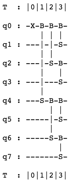
We can now describe the circuit itself. We start by putting the first qubit in state $\mathinner{|{1}\rangle}$ , while the remaining $d-1$ qubits remain in state $\mathinner{|{0}\rangle}$ . Then, we use the first parameter $\theta_{1}$ in an $RBS$ gate in order to “split” this ‘1’ between the first and the $d/2$ -th qubit. Then, we use the next two parameters $\theta_{2},\theta_{3}$ for the next layer of two $RBS$ gates, where again in superposition we “split” the ‘1’ into the four qubits with indices $(1,d/4,d/2,3d/4)$ and this continues for exactly $\log d$ layers until at the end of the circuit we have created exactly the state

\mathinner{|{x}\rangle}=\frac{1}{\left\lVert x\right\rVert}\sum_{i=1}^{d}x_{i}\mathinner{|{e_{i}}\rangle}

(2)

where the states $\mathinner{|{e_{i}}\rangle}$ are a unary representations of the numbers $1$ to $d$ , using $d$ qubits. The circuit appears in Fig. 1.

Refer to caption — Figure 1: The data loader circuit for an 8-dimensional data point. The angles of the $RBS(\theta)$ gates starting from left to right and top to bottom correspond to $(\theta_{1},\theta_{2},\ldots,\theta_{7})$ .

An interesting extension of our loader is that we can trade off qubits with depth and keep the number of overall gates $d-1$ (in this case, both $RBS$ and controlled- $RBS$ gates). For example, we can use $2\sqrt{d}$ qubits and $O(\sqrt{d}\log d)$ depth Ker2020. The circuit is quite simple, if one thinks of the $d$ dimensional vector as a $\sqrt{d}\times\sqrt{d}$ matrix. Then, we can index the coordinates of the vector using two registers (one each for the row and column) and create the state

\mathinner{|{x}\rangle}=\frac{1}{\left\lVert x\right\rVert}\sum_{i,j=1}^{\sqrt{d}}x_{ij}\mathinner{|{e_{i}}\rangle}\mathinner{|{e_{j}}\rangle}

For this circuit, we find, in the same way as for the parallel loader, the values $\theta$ and then create the following circuit in Figure 2. We start with a parallel loader for a $\sqrt{d}$ -dimensional vector using the first $\sqrt{d}$ angles $\theta$ (which corresponds to a vector of the norms of the rows of the matrix) and then, controlled on each of the $\sqrt{d}$ qubits we perform a controlled parallel loader corresponding to each row of the matrix.

Notice that naively the depth of the circuit is $O(d\log d)$ , but it is easy to see that one can interleave the gates of the controlled-parallel loaders to an overall depth of $O(\sqrt{d}\log d)$ . We will not use this circuit here but such circuits can be useful both for loading vectors and in particular matrices for linear algebraic computations.

Let us make some remarks about the data loader circuits. First, we will see in the following sections that the circuits are quite robust to noise and amenable to efficient error mitigation techniques. Second, we use a single type of two-qubit gate that is native or quasi-native to different hardware platforms. Third, we note that the connectivity of the circuit is quite local, where most of the qubits interact with very few qubits (for example $7/8$ of the qubits need at most 4 neighboring connections) while the maximum number of interacting neighbors for any qubit is $\log d$ . Here, we take advantage of the full connectivity of the ionQ hardware platform, so we can apply all gates directly. On a grid architecture one would need to embed the circuit on the grid which asymptotically requires no more than doubling the number of qubits.

Distance estimation circuit

Given two vectors ${x}$ and ${y}$ corresponding to classical data points, the Euclidean distance, namely $l_{xy}=\left\lVert{x}-{y}\right\rVert$ Ker2020 is given by

\displaystyle l_{xy}=\sqrt{\left\lVert{x}\right\rVert^{2}+\left\lVert{y}\right\rVert^{2}-2\left\lVert{x}\right\rVert\left\lVert{y}\right\rVert c_{xy}},

(3)

where $c_{xy}=\langle x|y\rangle$ is the inner product of the two normalised vectors. Here we describe a circuit to estimate $c_{xy}$ which is combined with the classically calculated vector norms to obtain $l_{xy}$ .

The power of the data loaders comes from the operations that one can do once the data is loaded into such “amplitude encoding” quantum states. In this work, we show how to use the data loader circuits to perform a fundamental operation at the core of supervised and unsupervised similarity-based learning, which is the estimation of the distance between data points.

In fact, here we will only discuss one of the variants of the distance estimation circuits which works for the case where the inner product between the data points is positive, which is usually the case for image classification where the data points have all non negative coordinates. It is not hard to extend the circuit with one extra qubit to deal with the case of also non-positive inner products.

The distance estimation circuit for two data points of dimension $d$ uses $d$ qubits, $2(d-1)$ two-qubit parametrized gates, $2\log d$ depth, and will allow us to measure at the end of the circuit a qubit whose probability of giving the outcome $\mathinner{|{1}\rangle}$ is exactly the square of the inner product between the two normalized data points. From this, one can easily estimate the inner product and the distance between the original data points. When the hardware allows deeper quantum operations, then an amplitude estimation procedure can be used to decrease the number of samples one needs to perform this estimation. For our experiments, we directly repeatedly measured the output state between 500-1000 times in order to get an estimate of the inner product.

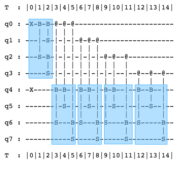
The distance estimation circuit is shown in Fig. 3, and it consists of two parts, the first is the data loader circuit for the first data point, and the second part is the adjoint data loader circuit for the second data point (without the $X$ gate), where we recall that for the adjoint $RBS^{\dagger}(\theta)=RBS(-\theta)$ . We can easily see that the probability the first qubit is measured in state $\mathinner{|{1}\rangle}$ is exactly the square of the inner product of the two data points.

After the first part, the state of the circuit is $\mathinner{|{x}\rangle}$ , as in Eq. 2. One can rewrite this state in the basis $\{\mathinner{|{y}\rangle},\mathinner{|{y^{\bot}}\rangle}\}$ as

\braket{x,y}\mathinner{|{y}\rangle}+\sqrt{1-|\braket{x,y}|^{2}}\mathinner{|{y^{\bot}}\rangle}

Once the state goes through the inverse loader circuit for $y$ the first part of the superposition gets transformed into the state $\mathinner{|{e_{1}}\rangle}$ (which would go to the state $\mathinner{|{0}\rangle}$ after an $X$ gate on the first qubit), and the second part of the superposition goes to a superposition of states $\mathinner{|{e_{j}}\rangle}$ orthogonal to $\mathinner{|{e_{1}}\rangle}$

\braket{x,y}\mathinner{|{e_{1}}\rangle}+\sqrt{1-|\braket{x,y}|^{2}}\mathinner{|{e_{1}^{\bot}}\rangle}

It is easy to see that after measuring the circuit (either all qubits or just the first qubit), the probability of getting $\mathinner{|{1}\rangle}$ in the first qubit is exactly the square of the inner product of the two data points.

We can also notice a simplification we can make in the circuit that will reduce the number of gates and depth. In the middle of the circuit, there are pairs of $RBS$ gates that are applied to the same consecutive qubits. Each such pair of two gates can be combined to one gate whose parameter $\theta$ is just equal to $\theta_{1}+\theta_{2}$ , where $\theta_{1}$ is the parameter of the first gate and $\theta_{2}$ is the parameter of the second gate.

This reduces the number of gates of the circuit to $3d/2-2$ and reduces the depth by one. The final circuit used in our application is in Fig. 4.

II.2 The Quantum Nearest Centroid classifier

II.2.1 Algorithm and software development

We now have all the necessary ingredients to implement the quantum Nearest Centroid classification circuit. As we have said, this is but a first, simple application of the above tools which can readily be used for other machine learning applications such as nearest neighbor classifiers or k-means clustering. Let us start by briefly defining the Nearest Centroid algorithm in the classical setting. The first part of the algorithm is to use the training data to fit the model. This is a very simple operation of finding the average point of each class of data, meaning one adds all points with the same label and finds the “centroid” of each class. This part will be done classically and one can think of this cost as a one-time offline cost.

In the quantum case, one will still find the centroids classically and then also pre-process them to find the parameters for the gates of the data loader circuits for each one of them and their norms. This does not change the asymptotic time of this step.

We will now look at the second part of the Nearest Centroid algorithm which is the “predict” phase. Here, we want to assign a label to a number of test data points and for that we first estimate the distance between each data point and each centroid and for each data point we assign the label of the centroid which is nearest to it.

The quantum Nearest Centroid is rather straightforward, it follows the steps of the classical algorithm apart from the fact that whenever one needs to estimate the distance between a data point and a centroid, we do this using the distance estimator circuit defined above.

The development of the quantum software followed one of the most popular classical ML libraries, called scikit-learn (https://scikit-learn.org/), where a classical version of the Nearest Centroid algorithm is available. In the code snippet below we can see how one can call the quantum and classical Nearest Centroid algorithm with synthetic data (one could also use user-defined data) through QCWare’s platform Forge, in a jupyter notebook.

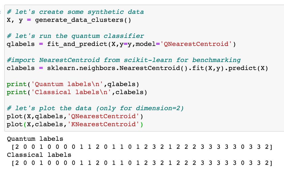
The function fit-and-predict first classically fits the model. For the prediction it calls a function distance-estimation for each centroid and each data point. The distance-estimation function runs the procedure we described above, using the function loader for each input and returns an estimate of the Euclidean distance between each centroid and each data point. The label of each data point is assigned as the label of the nearest centroid.

Note that one could imagine more quantum ways to perform the classification, where, for example, instead of estimating the distance for each centroid separately, this operation could happen in superposition. This would make the quantum algorithm faster but also increase the number of qubits needed. We remark also that the distance or inner product estimation procedure can find many more applications such as matrix-vector multiplications during clustering or training neural networks.

II.2.2 Runtime and Scalability

One of the main advantages of using the Nearest Centroid as a basic benchmark for quantum machine learning is that we fully understand what the quantum algorithm does and how its runtime scales with the dimension of the data and the size of the data set.

The quantum advantage comes from the distance estimation procedure which is based on the data loader circuits. As we have described, the circuit for estimating the distance of two $d$ -dimensional data points has depth $2\log d$ . Theoretically, for an estimation of the distance up to $\epsilon$ one needs to run the circuit $N_{s}=O(1/\epsilon^{2})$ times. Note also, that in the future one will be able to use amplitude estimation on top of this circuit in order to reduce the overall time to $O(\log d/\epsilon)$ . The accuracy required depends on how well-classifiable our data set is, meaning whether most points are close to a centroid or they are mostly distributed equidistantly from the centroids. This number does not really depend on the dimension of the data set and in all data sets we considered an approximation to the distance up to $0.1$ for most points and $0.03$ for a few difficult to classify points suffices, even for the full-scale MNIST dataset of 784 dimensions. Thus we expect that the number of shots will not significantly change as the problem sizes scale up.

Since the cost of calculating the circuit parameters is a one-off cost, if we want to estimate the distance between $k$ centroids and $n$ data points all of dimension $d$ , then the quantum circuits will need $d$ qubits and the running time would be of the form $O(kd+nd+kn\log(d/\epsilon))$ . The first term corresponds to pre-processing the centroids, the second term to pre-processing the new data points and the third term to estimating the distances between each data point and each centroid and assigning a label. The basic classical Nearest Centroid algorithm takes time $O(nkd)$ . One can design different classical Nearest Centroid algorithms that also sample using special data structures which will still be quadratically worse than a fully quantum one, at least with respect to the error.

We note that we do not claim here that the quantum Nearest Centroid procedure is faster than the classical one right now or that it will be in the very near future. Our goal is to measure the performance of the quantum routines outlined above on real hardware and real data. Procedures like the data loader circuits will be useful in the future as an input to much more classically complicated procedures including training neural networks or performing Principal Component or Linear Discriminant Analysis. An important outcome from this is the development of noise models and error mitigation techniques that will also help in improving and predicting the accuracy of the more complicated algorithms.

III Experiment

III.1 Trapped ion quantum computer

Our experimental demonstration is performed on an 11-qubit trapped ion processor based on ¹⁷¹Yb⁺ ion qubits. The device is commercially available through IonQ’s cloud service.

The 11-qubit device is operated with automated loading of a linear chain of ions (see figure 6), which is then optically initialized with high fidelity. Computations are performed using a mode-locked $355$ nm laser, which drives native single-qubit-gate (SQG) and two-qubit-gate (TQG) operations. The native TQG used is a maximally entangling Molmer Sorensen gate.

In order to maintain consistent gate performance, calibrations of the trapped ion processor are automated. Additionally, phase calibrations are performed for SQG and TQG sets, as required for implementing computations in queue and to ensure consistency of the gate perfomance.

III.1.1 Implementation of the circuits on the ionQ processor

The circuits we described above are built with the $RBS(\theta)$ gates (Eq. 1). To map these gates optimally onto the hardware we will instead use the modified gate

iRBS(\theta)=\left(\begin{array}[]{cccc}1&0&0&0\\ 0&\cos\theta&-i\sin\theta&0\\ 0&-i\sin\theta&\cos\theta&0\\ 0&0&0&1\end{array}\right)

(4)

It is easy to see that the distance estimation circuit stays unchanged. Using the fact that $iRBS(\theta)=\exp(i\theta(\sigma_{x}\otimes\sigma_{x}+\sigma_{y}\otimes\sigma_{y}))$ , we can decompose the gate into the circuit shown in Fig. Vatan2004. Each CNOT gate can be implemented with a maximally entangling Molmer Sorensen gate and single qubit rotations native to IonQ hardware.

We run 4 and 8 qubit versions of the algorithm. The 4 qubit circuits have 12 TQG and the 8 qubit circuits have 30 TQG.